1

FINITE ELEMENT ANALYSIS OF SHELL LIKE STRUCTURES USING IMPLICIT BOUNDARY METHOD

By

PREM DHEEPAK SALEM PERIYASAMY

A THESIS PRESENTED TO THE GRADUATE SCHOOL OF THE UNIVERSITY OF FLORIDA IN PARTIAL FULFILLMENT

OF THE REQUIREMENTS FOR THE DEGREE OF MASTER OF SCIENCE

UNIVERSITY OF FLORIDA

2009

2

© 2009 Prem Dheepak Salem Periyasamy

3

To Dr. Ramya Baby, Muthuraman, Shardha, Mr. Muthusamy, Mr. Arumugam, Dr. Ashok V.Kumar, Dr. Nam-Ho Kim, Dr. John Kenneth Schueller, God, Ravi Burla, Avdhut Joshi, Arjun

Ramachandran, Vivek Raju, to my roommates and other friends, to my other family members and my relatives

4

ACKNOWLEDGMENTS

I would like to express my sincere gratitude to my advisor and chairman of my supervisory

committee, Dr.Ashok V.Kumar, for his guidance, encouragement, enthusiasm and constant

support throughout my research. I would like to thank him for the numerous insights he provided

during every stage of my research. Without his assistance it would not have been possible to

complete this dissertation.

I would like to thank the members of my supervisory committee, Dr. Nam-Ho Kim and Dr.

John Kenneth Schueller. I am grateful for their willingness to serve on my committee, for

providing help whenever required, for involvement, for reviewing and valuable suggestions

during my thesis.

I would also like to thank my colleagues at Design ad Rapid Prototyping Laboratory at the

University of Florida for their help and support. I would especially thank Ravi Burla, Sung Uk-

Zhang, Nitin Chandola, Mittu Pannala and Anand Parthasarathy.

I would like to thank Ramya Baby, Muthuraman, and Sharadha for their constant love and

support. I would like to thank Mr. Muthusamy, Mr. Arumugam for their help and support.

Without them this would not have been possible. I would like to thank my friends Avdhut Joshi,

Arjun Ramachandran, Vivek Raju and other friends for their constant support. Last but not the

least; I would like to thank God for giving me this opportunity.

5

TABLE OF CONTENTS page

ACKNOWLEDGMENTS.................................................................................................................... 4

LIST OF TABLES................................................................................................................................ 7

LIST OF FIGURES .............................................................................................................................. 8

ABSTRACT ........................................................................................................................................ 11

CHAPTER

1 INTRODUCTION....................................................................................................................... 13

Overview ...................................................................................................................................... 13 Goals and Objectives .................................................................................................................. 16 Outline.......................................................................................................................................... 16

2 PLATE AND SHELL THEORY ............................................................................................... 18

Plate Theories .............................................................................................................................. 18 Formulation of Mindlin-Reissner Theory .......................................................................... 19 Constitutive Equation for Plate ........................................................................................... 21

Shells as an Assembly of Flat Elements .................................................................................... 23 Stiffness of a Plane Element in Local Coordinates ........................................................... 23 Transformation to Global Coordinates and Assembly of the Elements ........................... 25 Types of Planar Elements .................................................................................................... 26

Shear Locking .............................................................................................................................. 27 Reissner–Mindlin Elements ........................................................................................................ 28

Bathe–Dvorkin Element ...................................................................................................... 28 Discrete Kirchhoff Triangle Element (DKT) ..................................................................... 28 Discrete Shear Triangle Element (DST) ............................................................................ 29

3 IMPLICIT BOUNDARY FINITE ELEMENT METHOD ...................................................... 30

Finite Element Method ............................................................................................................... 30 Meshless Methods ....................................................................................................................... 31 Structured Grid Methods ............................................................................................................ 32 Implicit Boundary Finite Element Method (IBFEM) ............................................................... 33

Solution Structure for Imposing Essential Boundary Condition ...................................... 34 Dirichlet Functions .............................................................................................................. 36 Modified Weak Form for Linear Elasticity ........................................................................ 37 B-spline Interpolation .......................................................................................................... 38

One dimensional B-spline elements ............................................................................ 39 Two and three dimensional B-spline elements........................................................... 42

Advantages of IBFEM ................................................................................................................ 44

6

4 SHELLS USING IMPLICIT BOUNDARY METHOD .......................................................... 45

Linear Elastic Problems .............................................................................................................. 45 Formulation of Stiffness Matrix ......................................................................................... 46 Formulation of Stiffness Matrix for Elements with Essential Boundary Conditions ...... 47 Element Force/Load Formulation ....................................................................................... 50

5 ANALYSIS AND RESULTS .................................................................................................... 53

Flat Shell Problems ..................................................................................................................... 53 Cantilever Shell Problem .................................................................................................... 54 Simply Supported Shell Problem........................................................................................ 57 Centrally Loaded Square Clamped Plate in Bending ........................................................ 60

Obstacle Course Benchmark Problems...................................................................................... 63 Barrel Vault Roof Problem ................................................................................................. 63 Pinched Hemisphere Problem ............................................................................................. 68 Pinched Cylinder Problem .................................................................................................. 72

Micro Air Vehicle Wing ............................................................................................................. 76

6 CONCLUSION ........................................................................................................................... 80

Conclusions ................................................................................................................................. 80 Scope for Future Work................................................................................................................ 81

LIST OF REFERENCES ................................................................................................................... 82

BIOGRAPHICAL SKETCH ............................................................................................................. 86

7

LIST OF TABLES

Table page 5-1 Cantilever shell: results for vertical displacement at the end of cantilever shell, based

on various meshes and element types ................................................................................... 56

5-2 Simply supported shell: results for vertical displacement at the middle of the shell, based on various meshes and element types ......................................................................... 60

5-3 Square plate: results for vertical displacement at the middle of the square plate, based on various meshes and element types ................................................................................... 63

5-4 Barrel vault roof: results for vertical displacement at the middle of the free edge, based on various meshes and element types ......................................................................... 67

5-5 Pinched hemisphere: results for radial displacement at loaded points of hemisphere, based on various meshes and element types ......................................................................... 71

5-6 Pinched cylinder: results for vertical displacement at the midpoint of the cylinder, based on various meshes and element types ......................................................................... 75

8

LIST OF FIGURES

Figure page 1-1 Comparison between FEM mesh and IBFEM mesh for shells ........................................... 15

2-1 Flat element ............................................................................................................................ 24

2-2 Types of planar elements ....................................................................................................... 27

2-3 Example of a Timoshenko beam ........................................................................................... 27

3-1 Structured grid used in IBFEM ............................................................................................. 34

3-2 Solution structure for imposing essential boundary conditions in IBFEM ........................ 36

3-3 A one dimensional B-spline example ................................................................................... 40

3-4 Shape function of one dimensional quadratic B-spline element ......................................... 41

3-5 Shape function of one dimensional cubic B-spline element................................................ 42

3-6 A two dimensional quadratic B-spline element in parametric space .................................. 43

3-7 A two dimensional cubic B-spline element in parametric space ........................................ 44

4-1 Shells using IBFEM ............................................................................................................... 45

4-2 Representation of narrow band in element with essential boundary condition .................. 49

5-1 Cantilever shell ....................................................................................................................... 54

5-2 IBFEM result (continuous displacement plot) for cantilever shell example using cubic B-spline 64 node elements (10 Elements) .................................................................. 54

5-3 IBFEM result (continuous displacement plot) for cantilever shell example using quadratic B-spline 27 node elements (20 Elements) ............................................................ 55

5-4 Abaqus result for cantilever shell example using S4R (25 Elements using continuous displacement plot) .................................................................................................................. 55

5-5 ProMechanica result (continuous displacement plot) for cantilever shell example using shell type model for analysis (unknown mesh/element type) ................................... 56

5-6 Simply supported shell ........................................................................................................... 57

5-7 IBFEM result (continuous displacement plot) for simply supported shell example using cubic B-spline 64 node elements (10 Elements) ........................................................ 58

9

5-8 IBFEM result (continuous displacement plot) for square plate example using quadratic B-spline 27 node elements (40 Elements) ............................................................ 58

5-9 Abaqus result for simply supported shell example using shell type model for analysis S4R (900 Elements using continuous displacement plot) ................................................... 59

5-10 ProMechanica result (continuous displacement plot) for simply supported shell example using shell type model for analysis (unknown mesh/element type) .................... 59

5-11 Centrally loaded square plate ................................................................................................ 61

5-12 IBFEM result (continuous displacement plot) for square plate example using cubic B-spline 64 node elements (5 x 5 Mesh) with 0.1% error ................................................... 61

5-13 IBFEM result (continuous displacement plot) for square plate example using quadratic B-spline 27 node elements (40 x 40 Mesh) with 0.1% error .............................. 62

5-14 Abaqus result for square plate example using S4R (10 x 10 Mesh) with 0% error (continuous displacement plot) ............................................................................................. 62

5-15 Barrel vault roof ..................................................................................................................... 64

5-16 IBFEM result (continuous displacement plot) for barrel vault roof example using cubic B-spline 64 node elements (4 x 4 Mesh) with 0.1% error ......................................... 65

5-17 IBFEM result (continuous displacement plot) for barrel vault roof example using quadratic B-spline 27 node elements (9 x 9 Mesh) with 0% error...................................... 65

5-18 Abaqus result (continuous displacement plot) for barrel vault roof example using S8R5 (9 x 9 Mesh) with 0.6% error (other quarter modeled with different CSYS) from the Abaqus benchmark examples ................................................................................. 66

5-19 ProMechanica result (continuous displacement plot) for barrel vault roof example using shell type model for analysis with 0.9% error (unknown mesh/element type) ........ 66

5-20 Strain energy convergence plot ............................................................................................. 67

5-21 Pinched hemisphere ............................................................................................................... 68

5-22 IBFEM result (continuous displacement plot) for pinched hemisphere example using cubic B-spline 64 node elements (20 x 20 Mesh) with 10.3% error ................................... 69

5-23 IBFEM result (continuous displacement plot) for pinched hemisphere example using quadratic B-spline 27 node elements (40 x 40 Mesh) with 9.2% error .............................. 69

5-24 Abaqus result (continuous displacement plot) for pinched hemisphere example using S8R5 (8 x 8 Mesh) with 0% error from the Abaqus benchmark examples ........................ 70

10

5-25 ProMechanica result (continuous displacement plot) for pinched hemisphere example using shell type model for analysis with 0.1% error (unknown mesh/element type) ................................................................................................................ 70

5-26 Strain energy convergence plot ............................................................................................. 71

5-27 Pinched cylinder ..................................................................................................................... 72

5-28 IBFEM result (continuous displacement plot) for pinched cylinder example using cubic B-spline 64 node elements (20 x 20 Mesh) with 0.2% error ..................................... 73

5-29 IBFEM result (continuous displacement plot) for pinched cylinder example using quadratic B-spline 27 node elements (20 x 20 Mesh) with 4.9% error .............................. 73

5-30 Abaqus result (continuous displacement plot) for pinched cylinder example using S4R (20 x 30 Mesh) with 0.4% error from the Abaqus benchmark examples................... 74

5-31 ProMechanica result (continuous displacement plot) for pinched cylinder example using shell type model for analysis with 0.4% error (unknown mesh/element type) ........ 74

5-32 Strain energy convergence plot ............................................................................................. 75

5-33 Micro air vehicle wing ........................................................................................................... 76

5-34 IBFEM result (continuous displacement plot) for micro air vehicle wing example using cubic B-spline 64 node elements (10 x 5 Mesh) with 1.4% error ............................. 77

5-35 IBFEM result (continuous displacement plot) for micro air vehicle wing example using quadratic B-spline 27 node elements (10 x 10 Mesh) with 7% error ....................... 77

5-36 Abaqus result (continuous displacement plot) for micro air vehicle wing example using S8R5 (542 elements) with 0.5% error......................................................................... 78

5-37 ProMechanica result (continuous displacement plot) for micro air vehicle wing example using Shell type model for analysis with 52% error (unknown mesh/element type)......................................................................................................................................... 78

11

Abstract of Thesis Presented to the Graduate School of the University of Florida in Partial Fulfillment of the

Requirements for the Degree of Master of Science

FINITE ELEMENT ANALYSIS OF SHELL LIKE STRUCTURES USING IMPLICIT BOUNDARY METHOD

By

Prem Dheepak Salem Periyasamy

August 2009 Chair: Ashok V. Kumar Major: Mechanical Engineering

Shells are structures whose thickness is small compared to their other dimensions. Finite

element method (FEM) is the most widely used tool for analysis of such structures and shell

elements are used to model such structures. The most basic shell element is a flat element which

is formulated based on the Mindlin-Reissner theory. The Mindlin-Reissner theory yields good

results for thick shells but under-predicts deflections for relatively thin shells. In other words, the

stiffness of the shell increases as the thickness decreases. This is due to shear locking. Various

techniques have been proposed in the past two decades to circumvent this problem and reduced

integration is known to be the best solution. FEM uses conforming meshes and automatic mesh

generation algorithms can be unreliable for complicated models. In order to avoid the problems

associated with mesh generation, several meshless methods and structured grid methods have

been proposed in the past two decades. In this thesis, a structured grid method called implicit

boundary finite element method (IBFEM) has been used for analysis of shell like structures.

Three dimensional elements that use uniform B-spline approximation schemes for representing

the solution are used to model shells. B-spline approximations can provide higher order solutions

that have tangent and curvature continuity whereas the traditional shell elements use bilinear

12

interpolations which do not even have tangent continuity. The advantages and disadvantages of

using IBFEM and B-spline approximation for shell analysis are studied in this thesis.

Numerical examples are presented to demonstrate the performance of shell elements using

IBFEM and B-spline approximation. The results are compared with numerically converged

solutions and traditional shell elements solutions to demonstrate the ability of the IBFEM shell

elements to solve various shell problems in engineering. Convergence studies show that shell

elements used in this thesis converges with fewer elements and nodes when compared to the 4-

node, 8-node and 9-node iso-parametric reduced integration shell elements used in FEM.

13

CHAPTER 1 INTRODUCTION

Overview

A shell can be defined as a structure with a thickness which is small compared to its other

dimensions. For example a pressure vessel, whose thickness is less than 1/10 of global structural

dimension generally, is modeled using shell elements. Applications of shells include, but are not

limited to, structures made using sheet metals, fuselages of airplanes, boat hulls and roof

structures in buildings. The primary difference between a shell structure and plate structure is

that, the shell structures are subjected to bending and in-plane forces (stretching) while the plate

structures are subjected to only bending. Also the shell structures can be either curved or flat

while the plate structures are always flat. The stresses in the thickness direction are negligible for

such shell-like structures. The finite element method (FEM) has been a successful tool for the

analysis of shell like structures.

Shell theories are extended from the traditional plate theories. There are two plate theories

which majorly contributed to the advancement of plate and shell analysis. They are thin plate

theory and thick plate theory. The thin plate theory is based on Kirchhoff’s assumption that the

rotation at any point in plate is the slope of deflection at the same point, i.e., ;x ydw dwdx dy

θ θ= =

where and x y are the planar axes of plate and w is deflection. This theory neglects shear strain

energy and requires 1C continuous interpolation or approximation of the solution. The thick plate

theory is based on Mindlin’s (Mindlin and Reissner, 1951) assumption that the deflection and

rotation at any point in the plate are independent of each other, i.e., if w(x,y) is the deflection,

and ,x yθ θ are the rotation about the x and y axis then ,x yθ θ are not necessarily the slope of w.

14

This assumption allows the plate elements to be 0C continuous because the weak form

derived using Mindlin’s assumption does not involve second derivatives of the deflection. The

most basic shell element is a flat element which is formulated based on the Mindlin plate theory.

A shell element should be capable of handling in-plane forces as well as bending forces. The 2D

plane stress elements can handle in-plane forces while the plate elements can handle bending

forces. Hence a flat shell element is formulated by combining these two elements (Flugge, 1960).

Curved structures are approximated by adequate number of flat elements (Zienkiewicz, 1967).

The flat shell element uses linear approximation which is typically 0C continuous.

The Mindlin plate theory is good for thick plates but under-predicts deflections for

relatively thin plates. When the thickness of the shell reduces, the shell based on Mindlin theory

tends to stiffen. This is called shear locking in plates and shells (Cook, Malkus, Plesha, 1989).

Various techniques have been proposed to circumvent shear locking. Reduced integration is the

best-known solution for shear locking (Hughes and Tezduyar, 1981). Increasing the order of the

polynomials used for the interpolation also improves the solution (Hartmann and Katz, 2007).

In traditional FEM, shell elements are two dimensional flat or curved elements that

approximate the geometry as shown in Figure 1-1(a). In this thesis, analyses of shells using

structured grids are studied. A structured grid is a non-conforming mesh and all the elements in

the grid are regular in shape (rectangles/cuboids). Figure 1-1(b) shows a shell modeled using a

3D structured grid where the shell geometry passes through the elements of the grid. A structured

grid is generated on top of the analysis geometry. The geometry is independent of the grid and

could be represented using equations or in a format imported from CAD model.

15

A B Figure 1-1. Comparison between FEM mesh and IBFEM mesh for shells. A) FEM mesh for shell like structures, B) IBFEM mesh for shell like structures

A structured grid is much easier to generate than a finite element conforming mesh.

Automatic mesh generation algorithms for FEM can be unreliable for complicated geometries

often resulting in poor or distorted elements and such distorted elements can cause large errors in

solution. Significant amount of user intervention is required which makes mesh generation the

most time consuming step in the design process. Moreover, the analysis geometry is

approximated using elements. These limitations associated with conforming mesh generation can

be avoided by using a structured grid for analysis which is a significant advantage over

traditional FEM.

The nodes of a structured grid are not guaranteed to lie on the analysis boundary, and

therefore the traditional methods used in FEM for applying essential boundary conditions cannot

be used. So a special technique called implicit boundary method (Padmanabhan and Kumar,

2007) is used to enforce essential boundary conditions. Solution structures for the implicit

boundary method are constructed by using the approximate Heaviside step functions based on

the implicit equations of the boundaries for exact imposition of essential boundary conditions.

The use of structured grids for analysis creates the possibility of using various approximation

schemes like B-splines and Hermite interpolations which provide at least 1C continuity in the

domain of interest. The following properties of B-splines make it desirable to use them for shell

16

analysis. B-splines basis functions have compact support like finite element shape functions and

lead to banded stiffness matrices. B-spline approximation also provides high order of continuity

and is capable of providing accurate solutions with continuous gradients across elements.

Burla and Kumar (Burla and Kumar, 2008) have used B-spline approximation scheme with

implicit boundary finite element method (IBFEM). IBFEM is extended to shell analysis in this

thesis. The performance and capabilities of IBFEM shell elements are studied by solving several

shell problems in structural analysis. Convergence analysis is also performed using several

examples to study the behavior of IBFEM shell elements and it has been demonstrated that

IBFEM shell elements provide accurate solutions with a fewer number of elements when

compared to traditional 4, 8 and 9 node iso-parametric reduced integration shell elements.

Goals and Objectives

The goal of this research is to study the shell elements based on B-spline approximation

using the implicit boundary finite element method and to develop a solution structure for

imposing essential boundary conditions.

The main objectives of this thesis are:

• To extend implicit boundary finite element method to shells and to use B-spline approximation for shell analysis

• To study the convergence behavior of shell problems using finite elements based on B-spline approximations

• To study the advantages and disadvantages of using implicit boundary finite element method and B-spline approximation for shells

Outline

The remaining portion of this thesis is organized as follows:

Chapter 2 discusses various traditional plate and shell theories from literature. Various

assumptions and the limitations such as shear locking are discussed.

17

Chapter 3 discusses several meshless methods and methods based on structured grid for

analysis from the literature. The implicit boundary finite element method and the use of B-spline

basis functions are discussed in detail.

Chapter 4 discusses the extension of implicit boundary finite element method and B-spline

approximation to shells. The formulation of the solution structure for imposing essential

boundary conditions is also presented.

Several shell problems from structural mechanics, obstacle course shell problems and

stress concentration problems are studied in chapter 5. Convergence analyses are also performed

using these shell problems to study the behavior of IBFEM shell elements in terms of accuracy

and efficiency.

In Chapter 6, conclusions are drawn based on the results of the finite element models from

chapter 5. Advantages and disadvantages of using the implicit boundary finite element method

and B-splines for shells are also discussed in this chapter. Scope of future work is also presented.

18

CHAPTER 2 PLATE AND SHELL THEORY

Thin plates and shells are structures whose thickness is small compared to their other

dimensions. The primary difference between a shell and plate is that the shells are subjected to

bending and in-plane forces (stretching) while the plates are subjected to only bending. Also,

shells can be either curved or flat while plates are always flat. Applications of thin plates and

shells include, but are not limited to, structures made using sheet metals, pressure vessels, and

fuselages of airplanes, boat hulls, chimney stacks, automobile parts and roof structures in

building. The introduction of thin shells made an important contribution to the development of

several branches of engineering. Some major fields of applications of shell analysis are structural

engineering, vehicle body structures, architecture and buildings, power and chemical engineering

and composite construction. The finite element method (FEM) has been a successful tool for the

analysis of plates and shells. Since shells elements are extension of plate elements, plate theories

and literature are discussed below.

Plate Theories

Some of the greatest contributions towards thin plate theory came from Kirchhoff in 1850.

Kirchhoff’s assumptions lead to the thin plate theory otherwise known Kirchhoff plate theory. In

this theory, the rotation at any point in plate is assumed to be the slope of the deflection at the

same point. For the plate to remain continuous and not ‘kink’, the continuity condition between

finite elements has to be imposed to both deflection and rotation ( ;x ydw dwdx dy

θ θ= = , where

and x y are the planar axes of plate and w is deflection). The drawback of this theory is that it is

valid only for very thin plates where shear strain is negligible.

19

Mindlin and Reissner (Mindlin and Reissner, 1951) developed the thick plate theory. This

theory differs from the thin plate theory in basic assumption that the lateral displacement and

rotation for any point in a plate are independent. At every node , and x yw θ θ are treated as the

unknown nodal variables where w is deflection, and and x yθ θ are the rotations about the x and y

axis (which are not necessarily the slope of w.). The plate elements based on Mindlin’s theory

are 0C continuous. This is an advantage of this theory because it is difficult to develop

interpolation that is 1C continuous. Therefore, it is easier to implement thick plate theory than the

thin plate theory. The Mindlin plate theory is good for thick plates but under-predicts deflections

for thin plates.

Formulation of Mindlin-Reissner Theory

Assumptions:

For every 2( , ) ,x y A R∈ ⊂ and ,2 2t tz − ∈

33

3

0 ,( , ) 1,2

( , )u z x y whereu w x yα α

σθ α

== − ==

(2-1)

In Eq. (2-1), t is the thickness of the plate, 1, 2α = represents the x and y axis

respectively, w is deflection and and x yθ θ are rotations about the z axis. The normal stress in

the z-direction ( 33σ ) which is neglected.

Weak Form for Linear Elasticity

By the principal of virtual work, the weak form for a boundary value in linear elasticity is

given as:

20

T T T

V S V

dV u t dS u b dVδε σ δ δ= +∫ ∫ ∫ (2-2)

In Eq. (2-2), δε is the virtual strain, uδ is the virtual displacement, σ is the Cauchy

stress tensor b is the body force and t is the traction. Substituting the assumptions (Eq. 2-1) in

the weak form for linear elasticity (Eq. 2-2), and simplifying them, we get, the weak form for

plate,

Weak form for Plate:

( ) ( ) ( )A A s

K m q dA C wF dA M wQ dsαβ αβ α α α α α αδ δγ δθ δ δθ δ− + = − + + − +∫ ∫ ∫ (2-3)

In Eq. (2-3), 2

2

( )

t

t

m z dzαβ αβσ−

= ∫ is the bending moment per unit length,

2

3

2

( )

t

t

q dzα ασ−

= ∫ is the shear force per unit length on the α face,

2

3 3

2

t

t

F b dz t−

= +∫.is applied pressure on the plate,

2

2

( )

t

t

M zt dzα α−

= ∫ is pressure (normal stress) on the plate,

2

3

2

t

t

Q t dz−

= ∫ is the prescribed bending moment per unit of length,

2

3

2

t

t

Q t dz−

= ∫ is the prescribed shear force per unit of length,

21

2

2

t

t

C zb dz ztα α α−

= − +∫ is the applied couple per unit of length,

tα is the sum of shear stresses on the top and bottom surface of the plate

Constitutive Equation for Plate

The constitutive equation for plate is same as the constitutive equation for plane stress.

11 11

22 22

12 12

2 02 0

0 0 [ ] C

σ λ µ λ εσ λ λ µ εσ µ γ

σ ε

+ = +

=

(2-4)

Where 2 1 2(1 )

E Eandνλ µν ν

= =− −

are known as Lame’s constants, E is Young’s modulus,

ν is Poison’s ratio, σ is the stress vector and ε is the strain vector. Substituting the

constitutive equation (Eq. 2-4), [ ] Cσ ε= , in the expression for m, we get,

32 22

2 2

[ ] [ ] [ ] [ ] 12

t t

bt t

tm C zdz C k z dz C k D kε− −

= = − = − = −∫ ∫ (2-5)

In Eq. (2-5), 3

[ ] [ ]12btD C= , and q can be re-written as

[ ] sq D γ= (2-6)

where 05[ ]

06s

tD

tµ

µ

=

. After substituting these new expressions for m and q (Eq.

2-5 and Eq.2-6) to the LHS of the weak form, the weak form for Mindlin plate is given as,

Weak Form for Mindlin Plate:

The weak form for Mindlin plate (Eq. 2-7) is used for analysis of traditional plate elements

in FEM.

22

[ ] [ ]

( ) ( )

T Tb s

A A

T T T T

A s

k D k dA D dA

C w F dA M w Q ds

δ δγ γ

δθ δ δθ δ

+

= − + + − +

∫ ∫

∫ ∫ (2-7)

The curvature can be written as,

1

1111 1,

11222 1,

12212 1, 1,

1 2

2 1

0 0 0 0 [ ]

2 0

xb

y e

y x

wxk Nk k N B X

xk N N

x x

θ

θθθ

θ θ

∂ ∂ ∂ = = = = ∂ ∂ ∂ + ∂ ∂

(2-8)

In Eq. (2-8), [ ]bB is the strain displacement matrix for bending and 12

kx x

βααβ

β α

θθ ∂∂= + ∂ ∂

.

11

1, 111 11

1, 12 122

2

0 [ ]

0x s

ey

wwN N

B XN Nw

θθγ θ

γγ θθ

θ

∂ − −∂ = = = = −∂ − ∂

(2-9)

In Eq. (2-9), [ ]sB is the strain displacement matrix for shear and wxαα

γ ∂=∂

is the shear

deformation,

[ ] [ ][ ][ ]

[ ] [ ][ ][ ]

b b b b

A

s s s s

A

K B D B dA

K B D B dA

=

=

∫

∫ (2-10)

In Eq. (2-10), [ ]bK is the stiffness matrix corresponding to bending and [ ]sK is the stiffness

matrix corresponding to the shear, 3

[ ] [ ]12btD C= and

05[ ]06s

tD

tµ

µ

=

.

23

Weak form in Matrix Notation:

Using Eq. (2-10), the weak form for Mindlin plates in the matrix notation can be written

as,

([ ] [ ]) ([ ] [ ])[ ]

T B S T A Se e e e e e e

e e e

X K K X X F KK X F

δ δ+ = +=

(2-11)

In Eq. (2-11), [ ] [ ] [ ] and B S A Se e e e e eK K K F F F= + = + . A

eF is the distributed load and

seF is the load contribution from shear. The stiffness matrix and the force vector for individual

elements can be computed and then they can be assembled to solve the equations for unknowns

like traditional FEM.

Shells as an Assembly of Flat Elements

The most basic shell element is a flat shell element. A shell element should be capable of

handling in plane forces as well as bending forces. The 2D plane stress elements are known to

handle in-plane forces while the plate elements discussed in the previous section, are known to

handle bending forces. Hence a flat shell element is formulated by combining these two

elements. The formulation for the flat shell element using traditional shell theory from literature

is discussed below (Flugge, 1960).

Stiffness of a Plane Element in Local Coordinates

Consider a flat element subjected simultaneously to ‘in-plane’ and bending forces. For, ‘in

plane’ (plane stress) forces, the state of strain is given by the nodal displacements u and v in x-

and y direction respectively at node i , and we know that,

[ ]

iep p ep pi

i

ipi

i

uK x f with x

v

Uf

V

= =

=

(2-12)

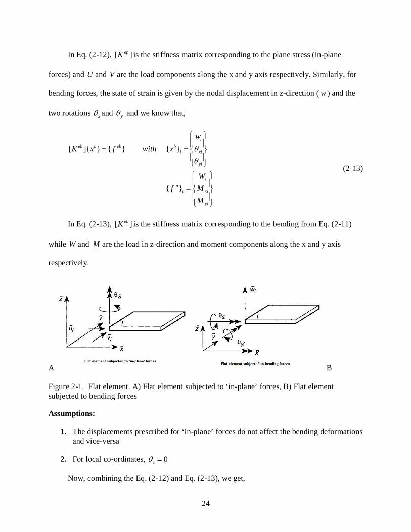
24

In Eq. (2-12), [ ]epK is the stiffness matrix corresponding to the plane stress (in-plane

forces) and U and V are the load components along the x and y axis respectively. Similarly, for

bending forces, the state of strain is given by the nodal displacement in z-direction ( w ) and the

two rotations xθ and yθ and we know that,

[ ]

ieb b eb b

i xi

yi

ip

i xi

yi

wK x f with x

Wf M

M

θθ

= = =

(2-13)

In Eq. (2-13), [ ]ebK is the stiffness matrix corresponding to the bending from Eq. (2-11)

while W and M are the load in z-direction and moment components along the x and y axis

respectively.

A B Figure 2-1. Flat element. A) Flat element subjected to ‘in-plane’ forces, B) Flat element subjected to bending forces

Assumptions:

1. The displacements prescribed for ‘in-plane’ forces do not affect the bending deformations and vice-versa

2. For local co-ordinates, 0zθ =

Now, combining the Eq. (2-12) and Eq. (2-13), we get,

25

[ ] rs eK x f= (2-14)

Eq. (2-14) includes stiffness,

0 0 0 00 0 0 0

0 0 0[ ] 0 0 0

0 0 00 0 0 0 0 0

prs

brs rs

K

K K

=

(2-15)

Nodal displacements,

i

ipi

ibi i

xizi

yi

zi

uv

xw

x xθ

θθθ

= =

(2-16)

and respective forces,

i

i

iei

xi

yi

zi

UVW

fMMM

=

(2-17)

The above formulation is valid for any polygonal element as shown in figure 2-1.

Transformation to Global Coordinates and Assembly of the Elements

A transformation of co-ordinates to a common global system which is denoted by xyz from

the local system (denoted by x y z′ ′ ′ ) is necessary to assemble the elements. The forces and

displacements of a node transform from the local to the global system is given by,

[ ] and [ ] i i i ix L x f L f′ ′= = (2-18)

In Eq. (2-18), 0

[ ]0

Lλ

λ

=

(2-19)

26

x x x y x z

y x y y y z

z x z y z z

λ λ λλ λ λ λ

λ λ λ

′ ′ ′

′ ′ ′

′ ′ ′

=

(2-20)

In Eq. (2-20), x xλ ′ = cosine of angle between x and x′ axes, etc. By the rules of orthogonal

transformation, the stiffness matrix of an element in global co-ordinate system can be given as,

e T eK T K T′= (2-21)

In Eq. (2-21),

0 00 00 0

LL

TL

=

(2-22)

[ ]T is a matrix made up of [ ]L matrices along the diagonal equal to the number of nodes in

the element. After the stiffness matrices of all the elements are determined, they are then

assembled into a global stiffness matrix and solved for the solution. The resulting displacements

correspond to the global co-ordinate system and have to be transformed to local co-ordinate

system for the stress computation (Zienkiewicz, 1967).

Types of Planar Elements

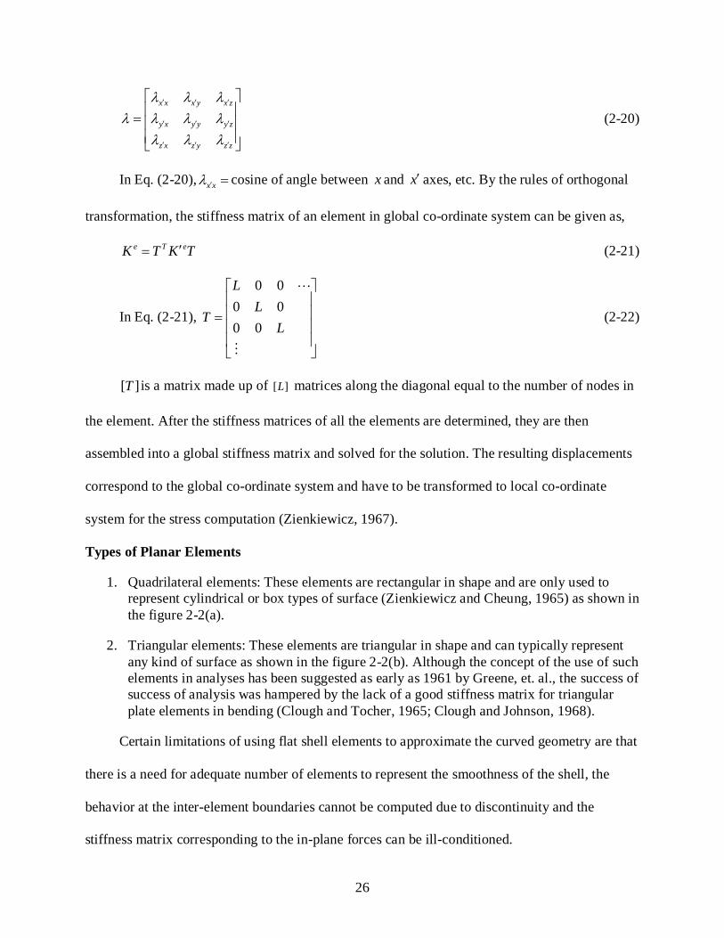
1. Quadrilateral elements: These elements are rectangular in shape and are only used to represent cylindrical or box types of surface (Zienkiewicz and Cheung, 1965) as shown in the figure 2-2(a).

2. Triangular elements: These elements are triangular in shape and can typically represent any kind of surface as shown in the figure 2-2(b). Although the concept of the use of such elements in analyses has been suggested as early as 1961 by Greene, et. al., the success of success of analysis was hampered by the lack of a good stiffness matrix for triangular plate elements in bending (Clough and Tocher, 1965; Clough and Johnson, 1968).

Certain limitations of using flat shell elements to approximate the curved geometry are that

there is a need for adequate number of elements to represent the smoothness of the shell, the

behavior at the inter-element boundaries cannot be computed due to discontinuity and the

stiffness matrix corresponding to the in-plane forces can be ill-conditioned.

27

A B Figure 2-2. Types of planar elements. A) Assembly of rectangular elements, B) assembly of triangular elements

Shear Locking

When the shell thickness shrinks, the Reissner–Mindlin plate tends to stiffen. This problem

is primarily due to numerical difficulties. If the shell equations could be solved exactly, then if

the thickness tends to zero the Reissner–Mindlin results should tend to the results of a Kirchhoff

plate (Cook, Malkus, Plesha, 1989).

Shear locking can be best explained by studying the example of a Timoshenko beam as

shown in the figure 2-3. For a short beam, the end deflection is identical to the exact solution.

But when the length l is much greater than the height h of the beam, the end deflection will be

much too small compared with the exact solution. This is due to shear locking.

Figure 2-3. Example of a Timoshenko beam

28

The reason for this stiffening effect is the different sensitivity of the bending stiffness and

the shear stiffness with respect to the height h of the beam. If the height h tends to zero, the

bending stiffness decreases much faster than the shear stiffness. Various techniques have been

proposed to circumvent shear locking and reduced integration is the best-known remedy (Hughes

and Tezduyar, 1981).

Reissner–Mindlin Elements

Numerous elements are proposed based on Reissner–Mindlin plate theory. The three most

popular elements are the Bathe–Dvorkin element, the DKT element and the DST element, are

discussed in this chapter.

Bathe–Dvorkin Element

Bathe–Dvorkin element was first developed by Hughes and Tezduyar (Hughes and

Tezduyar, 1981), and later extended by Bathe and Dvorkin (Bathe and Dvorkin, 1985) to shells.

The element is an iso-parametric four-node element with bilinear functions for the deflection w

and the rotations xθ and yθ . The shearing strains are calculated independent of the deflection at

the center and at the midpoint of edges. Hence the stiffness matrix only depends on the

deflections at the four corner points. The main advantage of this element is the easy transition

from thick shells to thin shells, so that the element is universally applicable.

DKT Element

The discrete Kirchhoff triangle (DKT) element can be considered a modified Kirchhoff

plate element or a modified Reissner–Mindlin plate element (Stricklin et. al. 1969). The element

is a triangular element. The first assumption is that for the rotations, linear functions are chosen

and the deflection is instead only defined along the edge and interpolated by Hermite

polynomials. The second assumption is that there are zero shearing strains at the corner points

29

and at the midside nodes. The latter assumption makes it possible to couple the rotations to the

deflection, and it is thereby possible to reduce the model to the three degrees of freedom at the

three corner points, so the result is a triangular plate element with the nine degrees of freedom.

The DKT element is very popular because with minimal effort ( 0C continuous) a triangular

element with the nodal degrees of freedom w , xθ and yθ is obtained. But this element is

nonconforming (Braess, 1997).

DST Element

DST elements are very similar to DKT elements (Batoz and Katili, 1992). The only

difference between DST and DKT elements is that, unlike DKT, the shearing strains are not zero

at the corner nodes of the triangle.

Although the shell finite elements today can produce good quality results without locking,

these results are achieved by using special techniques like reduced integration. Another approach

is to increase the order of the polynomials (Hartmann and Katz, 2007). In this thesis, the

behavior of quadratic and cubic B-spline based 3D shell elements is studied. The results obtained

using such shell elements are compared with the traditional shell elements.

30

CHAPTER 3 IMPLICIT BOUNDARY FINITE ELEMENT METHOD

Finite element method (FEM), various meshless methods and structured grid methods from

literature are briefly discussed in the first part of this chapter. A detailed discussion on implicit

boundary finite element method (IBFEM) is presented in the second part of this chapter.

Extension of IBFEM to uniform B-spline approximation is presented in the last part of this

chapter.

Finite Element Method

The finite element method (Hughes, 2000; Cook et. al. 2003) is a well established

numerical technique and is widely used in solving engineering problems in industry, as well as in

academia. In finite element analysis, the domain of analysis is subdivided into elements and the

resulting finite element mesh approximates the geometry and is also used to approximate the

solution by piece-wise interpolation within each element. Using Galerkin’s approach, the

governing differential equation in its strong form is converted into a weak form which is

approximated. This leads to a set of linear equations which can be solved using a sparse matrix

solver, skyline solver, etc. FEM has been applied to wide variety of physical problems in

linear/non-linear static and dynamic elasticity, steady state heat transfer, electrostatics and

magnetostatics.

In FEM, a conforming mesh is generated to approximate the shape of the analysis

geometry. Automatic mesh generation algorithms for FEM can be unreliable for complicated

geometries often resulting in poor or distorted elements and such distorted elements can cause

large errors in the solution. A significant amount of user intervention is required which makes

mesh generation the most time consuming step in the design process. In order to avoid these

31

problems with mesh generation, several methods have been proposed which can be classified

into two main categories: meshless methods and structured grid methods.

Meshless Methods

Various methods have been developed in the past two decades which avoid mesh

generation and such methods are referred as meshless or meshfree methods. Most of these

methods use only nodes that are not connected to form elements. Smoothed particle

hydrodynamics (SPH) is one of the first meshless methods in literature (Lucy, 1977; Gingold,

1982). This method uses Shepard shape functions as interpolants and uses a point collocation

method for discretization and nodal integration for stiffness matrix computation. The behavior of

the solution depends on the proper distribution of nodes. So there is a need to place the nodes

properly to avoid instability.

Element Free Galerkin Method was developed by Belytschko and his coworkers

(Belytschko et. al., 1994; Dolbow and Belytschko et. al., 1999). This method is based on a

moving least square approximation and uses a global Galerkin method for discretization.

Boundary conditions were applied using Lagrange multipliers which lead to an increased number

of algebraic equations and the stiffness matrix is not symmetric.

The Meshless Local Petrov-Galerkin (MLPG) method was developed by Atluri and his

coworkers (Atluri et al. 1999; Atluri and Zhu 2000a, 2000b). This method uses a moving least

square approximation and a Local Petrov-Galerkin weak form which is developed in the local

sub-domain. If the sub-domain intersects the boundary of the global domain, then the boundary

condition is applied on this local boundary by a penalty method. The advantages of this method

are that there is no need of special integration schemes or smoothing techniques and there is

flexibility in choosing the size and shape of the local domain. The drawbacks of this method are

that the stiffness matrices generated by this approach are not symmetric positive definite, the

32

penalty method imposes boundary conditions approximately, and there is the need to make sure

that the union of all the local domains should cover up the global boundary.

The Partition of unity method (PUFEM) uses a partition of unity functions to merge the

local approximation functions which represent the local behavior (Melenk and Babuska, 1996).

The main advantage of PUFEM is that the knowledge of the local behavior of solutions can be

used efficiently to get good numerical approximations. This method also yields good results in

the cases where FEM gives poor results or when FEM is computationally very expensive. One

drawback of this approach is that the stiffness matrix can be singular and the basis function needs

to be modified appropriately or special techniques are needed to solve the singular system.

The Generalized Finite Element Method (GFEM) was developed as a hybrid of the finite

element method and the Partition of Unity (Babuska et. al. 2002; Duarte et. al. 2000). The

desirable features like inter-element continuity and the Kronecker-delta property from FEM are

retained in GFEM.

The Natural element method developed by Sukumar (Sukumar et. al. 1998) uses the

natural neighbor interpolants which are based on a Voronoi tessellation of the nodes. These

interpolants are smooth over the whole domain except at the nodes where they are continuous.

The essential boundary conditions are applied on nodes for convex domains.

Structured Grid Methods

A number of techniques have been developed based on structured grids to approximate the

solution. The Extended Finite Element Method or X-FEM was developed by Belytschko and co-

workers (Belytschko et. al. 2003). This method uses implicit equations for definition of the

geometry of the analysis domain and the Dirichlet boundary conditions are applied using

Lagrange multipliers.

33

The Penalty boundary method developed by Clark and Anderson (Clark and Anderson,

2003a, 2003b) uses a regular structured grid and a constrained variational formulation to apply

essential boundary conditions using a penalty method.

Shapiro (Shapiro, 1998; Shapiro and Tsukanov, 1999) and Hollig (Hollig et. al. 2001;

Hollig and Reif 2003; Hollig 2003) used R-functions to define the boundary of the problem

domain and the solution structure proposed by Kantorovich and Krylov (Kantorovich and Krylov

1958) was constructed to satisfy Dirichlet boundary conditions. Shapiro used transfinite

Lagrange interpolation and R-functions to impose Dirichlet boundary conditions while Hollig

used weight functions based on distance functions and R-functions. Hollig developed extended

B-spline basis to represent the solution in the analysis domain.

The Implicit boundary finite element method (IBFEM) was developed by Padmanabhan

and Kumar (Padmanabhan, 2006 and Kumar et. al. 2007). In this approach, approximate

Heaviside step functions are used to construct a solution structure based on the technique

proposed by Kantorovich and Krylov (Kantorovich and Krylov, 1958). All the internal elements

in this method have identical stiffness matrices. Since shell analysis using IBFEM are studied in

this thesis, IBFEM is discussed in more detail below.

Implicit Boundary Finite Element Method

Implicit boundary finite element method (IBFEM) uses structured grid for discretizing the

analysis domain as shown in the figure 3-1. The grid is generated on top of the geometry such

that it overlaps the geometry. The geometry is represented independently using equations and is

not approximated by the grid. A typical structured grid used in IBFEM is shown in the figure 3-

1. Elements which lie completely inside the boundaries of the geometry are called internal

elements and the elements which lie partially inside and partially outside the boundary are called

34

the boundary elements. The boundary elements intersect the boundary of the geometry. The

nodes are equally spaced in all directions.

Figure 3-1. Structured grid used in IBFEM

The nodes of a structured grid are not guaranteed to lie on the analysis boundary. So a

special technique called implicit boundary method (Padmanabhan and Kumar, 2007) is used to

enforce essential boundary conditions. Solution structures for implicit boundary method are

constructed by using the approximate Heaviside step functions based on the implicit equations of

the boundaries for exact imposition of essential boundary conditions.

Solution Structure for Imposing Essential Boundary Condition

Essential boundary conditions are typically specified as displacements or temperatures on

the essential boundaries. Let u be the trial function defined over analysis domain Ω in 2R or 3R .

The solution structure is constructed such that the essential boundary condition u=a is satisfied in

continuum Ω. The trial function u based on the technique proposed by Kantorovich and Krylov

(Kantorovich and Krylov, 1958) can be given as,

u U aφ= ⋅ + (3-1)

35

The trial function in Eq. (3-1) is guaranteed to satisfy the boundary condition u a=

defined by the implicit equation 0φ = for any :U RΩ→ . The variable part U of the solution

structure is approximated by piece wise polynomial within the elements of the grid. Typically,

0φ = condition is satisfied along the whole boundary of the geometry while the essential

boundary conditions are needed to be imposed only along the essential boundary. Shapiro

(Shapiro, 1998; Shapiro and Tsukanov, 1999) used R-functions to define the boundary of the

problem domain such that φ takes a value of zero only at the essential boundary. Hollig (Hollig

et. al. 2001; Hollig and Reif 2003; Hollig 2003) used distance functions or R-functions to define

the boundary of the problem domain such that φ takes a value of zero only at the essential

boundary. Both Shapiro and Hollig used B-spline basis functions to represent the solution in the

analysis domain. Instead of using any implicit equation, Padmanabhan and Kumar

(Padmanabhan, 2006 and Kumar et. al. 2007) used Dirichlet function or simply D-function

which is an approximate step function in the solution structure. The advantage of using

approximate step function as D-function is that, for all the internal elements, the value of D-

function becomes unity, and hence the stiffness matrix of all the internal elements are identical.

The trial function u is assumed to be displacement in elasticity problems and temperature in heat

transfer problems. The trial function u can be approximately represented as,

g au Du u= + (3-2)

In Eq. (3-2), gu is the grid variable which varies across the elements of the grid, au is the

boundary value function which becomes ou at essential boundary. A boundary value function is a

piecewise continuous function which satisfies the specified values at the essential boundaries.

The trail function is graphically represented in the figure 3-2.

36

Figure 3-2. Solution structure for imposing essential boundary conditions in IBFEM

Dirichlet Functions

The Dirichlet function is a function whose value becomes zero on all essential boundaries

when 0φ = and when 0φ ≠ , the value increases to unity in a narrow region near the boundary

whose width isδ and then remains unity inside the continuum,Ω . In the implicit boundary finite

element method, the D-function is used as an approximate Heaviside step function by

considering the limit 0δ → . If the boundary is represented by implicit equation 0φ = , then the

step function at any given point x is defined as,

( )

00

1 1 0

1

k

Dφ

φφ φ δδ

φ δ

≤

= − − ≤ ≤ ≥

(3-3)

In the above expression, k is the order of D insideδ . For example, k is 2 for quadratic and

3 for cubic. The magnitude of 510δ −≈ or smaller is used in the implementation. When 0δ → , the

gradient of D increases inside the narrow region and is non zero at the essential boundary. This

37

expression is only valid for imposing essential boundary condition on single boundaryφ . When a

single essential boundary condition has to be imposed on multiple boundaries 1 2( , ,..., )nφ φ φ

passing through same element, then D-function has to be constructed as Boolean combination(s)

of individual step functions. The Boolean combinations may include union, intersection and

subtraction. For more than two boundaries within one boundary element, a Boolean tree similar

to a CSG tree is constructed.

Modified Weak Form for Linear Elasticity

By the principle of virtual work, the weak form for a boundary value in linear elasticity is

given as:

T T T

V S V

dV u t dS u b dVδε σ δ δ= +∫ ∫ ∫ (3-4)

In Eq. (3-3), δε is the virtual strain, uδ is virtual displacement, σ is Cauchy stress

tensor, b is body force and t is the traction. The trial function is represented as,

[ ] g a s au D u u u u= + = + (3-5)

In Eq. (3-4), [ ] s gu D u= and [ ] ( ,..., )di nD diag D D= is a diagonal matrix where iD are

D-functions that vanish on boundaries on which the thi component of displacement is specified

and dn is the dimension of problem, so,

[ ] [ ]( )

s a

s a s aC Cε ε ε

σ ε ε ε σ σ

= +

= = + = + (3-6)

Substituting Eq. (3-5) in weak form (Eq. 3-3), we get the modified weak form as,

T s T T T a

V S V V

dV u t dS u b dV dVδε σ δ δ δε σ= + −∫ ∫ ∫ ∫ (3-7)

38

The nodal values of displacement are approximated as g gi j iju N u= , where jN are the shape

functions and giju are the nodal values of the grid variable; i represent degree of freedom of field

variable and j represents number of nodes. The stress and virtual strain are expressed as

[ ][ ] s eC B Xσ = and [ ] eB Xδε δ= respectively, where [ ]B is the strain displacement

matrix, eXδ and eX are the nodal values of the grid variable for element e . Using the above

expressions, the modified weak form is discretized into a system of linear equations as expressed

below,

1 1 1 [ ] [ ][ ]

where, e

e e

NE NE NBEe T T e e T e e T T

e e eV S

e T T a

V V

X B C B X dV X F X N t dS

F N b dV B dV

δ δ δ

σ

= = =

= +

= −

∑ ∑ ∑∫ ∫

∫ ∫ (3-8)

In Eq. (3-7), (NE) is the total number of elements in grid and (NBE) is the total number of

boundary elements in grid. The element matrices are assembled together to form a global matrix

which represents set of linear equations. The left hand sides of the equations correspond to the

stiffness matrix and the right hand sides of the equations correspond to the load vectors. Unlike

FEM, there is a forcing term in the weak form which arises from the boundary value functions

and also nodal variables to be solved are grid variables and not displacements. Since no

assumptions are restricting the choice of shape functions used to represent the grid variables, this

approach can be used with a variety of interpolation schemes, such as B-spline approximations,

meshless approximations and Lagrange interpolation.

B-spline Interpolation

B-spline shape (basis) functions are traditionally constructed using a recursive definition

(Farin, 2002). The parameter space is partitioned into elements using a knot vector (equivalent to

39

a collection of nodes). General methods are available to insert knots and elevate the order of the

polynomial.

IBFEM was recently extended to B-spline approximation by Burla and Kumar (Burla and

Kumar, 2008). In this method, Lagrange interpolation is replaced by B-spline approximation for

representing the solution. A B-spline approximation leads to better solution quality and

continuity.

A B-spline interpolation can be classified into 2 types based on polynomial order and they

are Quadratic B-spline approximation and Cubic B-spline approximation. Quadratic B-splines

are C1 continuous (gradient continuous) and cubic B-splines are C2 continuous (curvature

continuous) while the conventional finite elements use Lagrange interpolation schemes which

are C0 continuous. B-spline approximation can also be categorized based on uniformity, and they

are uniform B-splines, non-uniform B-splines and non-uniform rational B-splines (NURBS).

One dimensional B-spline elements

The polynomial expressions for the basis functions are derived using the continuity

requirements between neighboring elements. Any thk order B-spline has 1k + support nodes. The

B-spline polynomials are expressed as, 0

kj

i ijj

N a r=

=∑ where ija are the coefficients which

determine the continuity requirements, the parameter range for any element is [ 1,1]r∈ − , the

parameter value for first support node is 12

kr += − and the parameter value for the ( 1)thk +

support node is 12

kr += with uniform parameterization.

The piecewise polynomial can be written as,

40

0 0 0

( )k k k

je i i ij i

i i jf r N u a r u

= = =

= =

∑ ∑ ∑ (3-9)

In Eq. (3-8), iu represents the values at the support nodes. The continuity requirements can

be mathematically satisfied using the condition below,

1(1) ( 1) , 0,1,..., 1m m

e em m

f f m kr r

+∂ ∂ −= = −

∂ ∂ (3-10)

In Eq. (3-9), the derivatives of any element e at 1r = are equated to their corresponding

derivatives of the ( 1)the + element at 1r = − . The order of derivatives limit to 1k − . Using this

continuity approach, the shape functions for quadratic and cubic B-splines can be derived as

shown below. A typical one-dimensional B-spline is shown in figure 3-3.

Figure 3-3. A one dimensional B-spline example

Quadratic B-spline Element. A quadratic B-spline element in one-dimension has three

nodes and therefore it is represented by three shape functions. The expression of the shape

functions are given below,

41

21

22

23

1 (1 2 )81 (6 2 )81 (1 2 )8

N r r

N r

N r r

= − −

= −

= + +

(3-11)

The plots of the shape functions in Eq. (3-10) are shown in figure 3-4.

Figure 3-4. Shape function of one dimensional quadratic B-spline element

Cubic B-spline Element. A cubic B-spline element in one-dimension has four nodes and

therefore it is represented by four shape functions. The expression of the shape functions are

given below,

2 31

2 32

2 33

2 34

1 (1 3 3 )481 (23 15 3 3 )481 (23 15 3 3 )481 (1 3 3 )48

N r r r

N r r r

N r r r

N r r r

= − + −

= − − +

= + − −

= + + +

(3-12)

42

The plots of the shape functions in Eq. (3-11) are shown in figure 3-5. This figure shows

that the B-splines are not unity at respective nodes and do not vanish at other nodes. This shows

that they do not satisfy the kronecker-delta property and they also do not interpolate nodal

values.

Figure 3-5. Shape function of one dimensional cubic B-spline element

Two and three dimensional B-spline elements

The shape functions for the higher dimensional B-spline elements are constructed by

taking product of the shape functions for one-dimensional B-splines. The elements used for grid

are regular quadrilaterals (rectangle/square) or regular hexahedra (cube/cuboid), so mapping for

geometry of elements from parametric space to the physical space is linear.

Quadratic B-spline Element. The shape functions for two and three-dimensional

quadratic B-splines are constructed as a product of one-dimensional quadratic B-splines. The

shape functions can be expressed as,

23( 1)

39( 1) 3( 1)

( , ) ( ) ( ); , 1, 2,3

( , , ) ( ) ( ) ( ); , , 1, 2,3

Dj i i j

Dk j i i j k

N r s N r N s i j

N r s t N r N s N t i j k− +

− + − +

= =

= = (3-13)

43

The plots of the shape functions in Eq. (3-12) are shown in figure 3-6. The geometry

mapping between parametric and physical space can be defined as below,

1 12 2

l ui ii i i

r rx x x− += + (3-14)

In Eq. (3-13), lix and u

ix are the lower and upper bounds respectively for nodal coordinates

of any given element.

Figure 3-6. A two dimensional quadratic B-spline element in parametric space

Cubic B-spline Element. The shape functions for two and three-dimensional cubic B-

splines are constructed by product of one-dimensional cubic B-splines. The shape functions can

be expressed as,

24( 1)

316( 1) 4( 1)

( , ) ( ) ( ); , 1, 2,3, 4

( , , ) ( ) ( ) ( ); , , 1, 2,3, 4

Dj i i j

Dk j i i j k

N r s N r N s i j

N r s t N r N s N t i j k− +

− + − +

= =

= = (3-15)

44

The plots of the shape functions in Eq. (3-14) are shown in figure 3-7. The geometry

mapping between parametric and physical space can be defined as the same way as equation (Eq.

3-13),

Figure 3-7. A two dimensional cubic B-spline element in parametric space

Advantages of IBFEM

Advantages of using IBFEM for engineering analysis are,

• The grid generation is simple and quick. The grid is non-conforming and structured and this property saves pre-processing time and removes the need for complicated mesh generation algorithms.

• Use of B-spline approximation improves the solution quality and continuity. For example, a problem whose exact solution is a 3rd degree polynomial can be accurately computed using cubic B-spline approximation.

These are some of the important motivating factors to study the behavior of shell elements

based on IBFEM using uniform B-spline approximation.

45

CHAPTER 4 SHELLS USING IMPLICIT BOUNDARY METHOD

The implicit boundary finite element method (IBM) is extended to shells to study the

behavior of elements based on B-spline approximation for shell analysis. The implementation of

shell elements is discussed in detail and the formulation of solution structure for imposing

essential boundary conditions is also presented.

A B Figure 4-1. Shells using IBFEM. A) Hemispherical solid geometry in IBFEM, B) Front view of a typical IBFEM grid used for analysis.

Linear Elastic Problems

Shell elements in linear elasticity are subjected to both in-plane and bending forces. All the

shell elements implemented in this thesis are three-dimensional regular hexahedra (cube/cuboid)

elements as shown in figure 4-1(b) and (c).

The modified weak form for linear elastic problems is discussed in last chapter and can is

expressed as,

T s T T T a

V S V V

dV u t dS u b dV dVδε σ δ δ δε σ= + −∫ ∫ ∫ ∫ (4-1)

From above expression (Eq. 4-1), the modified weak form is discretized into system of

equations as expressed below,

46

1 1 1 [ ] [ ][ ]

where, e

e e

NE NE NBEe T T e e T e e T T

e e eV S

e T T a

V V

X B C B X dV X F X N t dS

F N b dV B dV

δ δ δ

σ

= = =

= +

= −

∑ ∑ ∑∫ ∫

∫ ∫ (4-2)

The stiffness matrix can be expressed as [ ] [ ][ ]e

e T

V

K B C B dV= ∫ . The stiffness matrix is

computed individually for all the elements in grid and then assembled into a global stiffness

matrix before solving equations. A typical IBFEM grid used for shell analysis is shown in Figure

4-1. Since shells are modeled as open manifolds, there are no internal elements and all the

elements in the grid for shell analysis are boundary elements. Amongst all elements only some of

the elements contain essential boundary conditions and these elements need a special formulation

to impose essential boundary conditions. The computation of stiffness matrix for elements

without any boundary condition is discussed first.

Formulation of Stiffness Matrix

The shell geometry typically passes through the element. Only a portion of this element

that intersects with the volume of the shell contributes directly to the analysis domain. Therefore

special techniques are needed for computation of the stiffness matrix. The portion of shell

surface inside any element is subdivided into small triangles. The stiffness matrix of any element

is computed by adding the stiffness contribution from all the triangles as shown below:

1[ ] [ ]

tn

e ii

K K=

=∑ (4-3)

In Eq. (4-3), tn is the total number of triangles in any element e and [ ]iK is the stiffness

matrix contribution corresponding to the thi triangle. The stiffness matrix[ ] [ ] [ ][ ]i

Ti

V

K B C B dV= ∫

is computed using Gauss quadrature. Gauss quadrature is one of the most efficient numerical

47

techniques to evaluate integrals. For shells, the volume integration is evaluated as a combination

of area and thickness integration. It is evaluated as follows,

2

2

[ ] [ ] [ ][ ]i

h

Ti i

h A

K B C B dA dh−

=

∫ ∫ (4-4)

In Eq. (4-4), iA is the area of thi triangle and h is the thickness of the shell. The normals at

the corners of the triangle are known from the model geometry and are interpolated at Gauss

points to reduce the cumulative error due to triangulation.

Formulation of Stiffness Matrix for Elements with Essential Boundary Conditions

For the boundary elements containing essential boundary conditions, the D-functions are

used and the D-functions are defined over a narrow band of width 510δ −≈ . The gradients of D-

function over the narrow band can have large values. In order to accurately compute the

contribution of the D-function and its gradient to the stiffness matrix, a special technique is used-

that is discussed below. The trial function in this case is displacement and is represented as,

[ ] g a s au D u u u u= + = + (4-5)

In Eq. (4-5), [ ] s gu D u= , [ ] ( ,..., )di nD diag D D= is a diagonal matrix where iD are

components of D-functions and dn is the dimension of problem

The nodal values of displacement are approximated as g gi j iju N u= ,

[ ] [ ]

s T e

e e

u D N XB Xε

=

= (4-6)

In Eq. (4-6), [B] is the strain-displacement matrix can be expressed as,

48

1 11 1

1 1

1 23 2 2 1

2 2

1 1 1 21 1 2 1

2 2 1 1

0

[ ] 0

where, is the number of nodes

m

N DD Nx x

N DB D Nx x

N D N DD N D Nx x x x

m

×

∂ ∂+ ∂ ∂

∂ ∂= + ∂ ∂ ∂ ∂ ∂ ∂

+ + ∂ ∂ ∂ ∂

(4-7)

1 11 1

1 1

1 23 2 2 1

2 2

1 1 1 21 2 1 1

2 1 2 1

0 0

[ ] 0 0m

N DD Nx x

N DB D Nx x

N N D DD D N Nx x x x

×

∂ ∂ ∂ ∂ ∂ ∂

= + ∂ ∂ ∂ ∂ ∂ ∂

∂ ∂ ∂ ∂

(4-8)

1

1 1

1 11

2 123 2 2

11 21 2

2 1 2

1 2 1

1

0

00 0 00

[ ] 0 0 0000 0

0

m

Nx D

N xDx NDB D

NN xD D

x D DN x xx

×

∂ ∂ ∂ ∂ ∂ ∂ ∂ = + ∂ ∂ ∂ ∂ ∂ ∂ ∂ ∂ ∂

(4-9)

3 2 3 4 4 2 3 2 2 2[ ] [ ] [ ] [ ] [ ]m m mB D N D N× × × × ×= ∆ + ∆ (4-10)

1 2[ ] [ ] [ ]B B B= + (4-11)

In Eq. (4-11), 1[ ] [ ][ ]B D N= ∆ contains terms involving the gradient of shape functions and

2[ ] [ ][ ]B D N= ∆ contains terms involving the gradient of D-function.

Now,

( )1 2 [ ] [ ] e eB B Xε = + (4-12)

49

Substituting Eq. (4-12) in the stiffness matrix expression2

2

[ ] [ ] [ ][ ]i

h

Ti i

h A

K B C B dA dh−

= ∫ ∫ ,

( ) ( )2

1 2 1 2

2

[ ] [ ] [ ] [ ] [ ] [ ]i

h

Ti i

h A

K B B C B B dA dh−

= + +∫ ∫ (4-13)

Eq. (4-13) can be re-written as,

( )

2

1 1 1 2 2 1 2 2

2

1 2 2 3

[ ] [ ] [ ][ ] [ ] [ ][ ] [ ] [ ][ ] [ ] [ ][ ]

[ ] [ ] [ ] [ ]

i i i i

h

T T T Ti i i i i

h A A A A

T

K B C B dA B C B dA B C B dA B C B dA dh

K K K K

−

= + + +

= + + +

∫ ∫ ∫ ∫ ∫ (4-14)

The stiffness matrix can be decomposed into three main components as shown in equation

(Eq. 4-14). Here 1[ ]K contains terms involving only gradients of shape functions, so this

component can be computed by sub-dividing the geometry into triangles. 2[ ]K and 3[ ]K contain

terms involving gradients of D-functions and vanish in the shaded region shown in the figure 4-

2. The gradient of D-function is very large inside the narrow band and cannot be neglected.

Hence 2[ ]K and 3[ ]K are computed only in the narrow region from 0φ = toδ .

Figure 4-2. Representation of narrow band in element with essential boundary condition

50

( )2 2[ ] [ ]TK K+ contain terms involving both gradients of D-functions and gradients of

shape functions. The gradient of shape functions can be assumed to be constant across the band

but varies along the boundary while the gradient of D-function can be assumed to be constant

along the boundary but varies normal to the boundary. The boundary of shell geometry is sub-

divided into line segments. The second component of stiffness matrix 2[ ]K can be evaluated as a

combination of a line integral along the normal to the boundary and a line integral along the line

segment of the boundary and a line integral along the shell thickness. Hence 2[ ]K can be written

as,

2

2 1 2

2

2 21

1[ ] [ ] [ ][ ]

[ ] [ ]

j

l

h

Tj j

h l

n

jj

K B C B d dl dh

K K

φ

φφ

−

=

=∇

=

∫ ∫ ∫

∑

(4-15)

In Eq. (4-15), ln is the total number of line segments in the element e and 2[ ]jK is the

stiffness component of thj line segment. Similarly, the last term can be written as,

2

3 2 2

2

3 31

1[ ] [ ] [ ][ ]

[ ] [ ]

j

l

h

Tj j

h l

n

jj

K B C B d dl dh

K K

φ

φφ

−

=

=∇

=

∫ ∫ ∫

∑

(4-16)

The stiffness matrices of all the triangles are added to compute the stiffness matrix for its

corresponding element. The technique presented above is used to compute the stiffness matrix of

boundary elements containing essential boundary conditions.

Element Force/Load Formulation

The discretized form of the modified weak form in Eq. (4-2) is re-written below,

51

1 1 1 [ ] [ ][ ]

, e

e e

NE NE NBEe T T e e T e e T T

e e eV S

e T T a

V V

X B C B X dV X F X N t dS

where F N b dV B dV

δ δ δ

σ

= = =

= +

= −

∑ ∑ ∑∫ ∫

∫ ∫

The right hand side of the above expression contains two terms. The term eF

corresponds to volume integration for the body forces and applied non-homogenous essential

boundary conditions and the second term is a surface integration for the traction forces over the

natural boundaries.

The shell boundaries are approximated as a set of line segments and are evaluated using

Gauss quadrature as shown below,

2

2

1

i

l

h

Ti

h L

n

ii

f N t d dh

f f

−

=

= Γ

=

∫ ∫

∑

(4-17)

In Eq. (4-17), t is the traction acting on the natural boundary, the traction forces are

evaluated as combination of line integrals. The load is integrated along the boundary iL and

through thickness h . The traction forces for individual IBFEM shell elements can be computed

using the above formulation.

2

2

h

e T

h A

F N b dAdh−

= ∫ ∫ (4-18)

In Eq. (4-18), the body forces are evaluated as combination of line and area integrals. The

body forces are integrated along the surface of the geometry A and through thickness h . The body

forces for individual IBFEM shell elements can be computed using the above formulation.

52

Once the stiffness matrices of all the elements are computed individually, they are all

assembled to form a global stiffness matrix like traditional FEM and loads are distributed to the

nodes of the elements. Finally, they are solved using a sparse matrix solver.

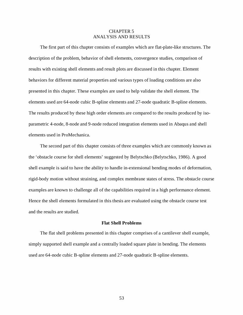
53

CHAPTER 5 ANALYSIS AND RESULTS

The first part of this chapter consists of examples which are flat-plate-like structures. The

description of the problem, behavior of shell elements, convergence studies, comparison of

results with existing shell elements and result plots are discussed in this chapter. Element

behaviors for different material properties and various types of loading conditions are also

presented in this chapter. These examples are used to help validate the shell element. The

elements used are 64-node cubic B-spline elements and 27-node quadratic B-spline elements.

The results produced by these high order elements are compared to the results produced by iso-

parametric 4-node, 8-node and 9-node reduced integration elements used in Abaqus and shell

elements used in ProMechanica.

The second part of this chapter consists of three examples which are commonly known as

the ‘obstacle course for shell elements’ suggested by Belytschko (Belytschko, 1986). A good

shell example is said to have the ability to handle in-extensional bending modes of deformation,

rigid-body motion without straining, and complex membrane states of stress. The obstacle course

examples are known to challenge all of the capabilities required in a high performance element.

Hence the shell elements formulated in this thesis are evaluated using the obstacle course test

and the results are studied.

Flat Shell Problems

The flat shell problems presented in this chapter comprises of a cantilever shell example,

simply supported shell example and a centrally loaded square plate in bending. The elements

used are 64-node cubic B-spline elements and 27-node quadratic B-spline elements.

54

Cantilever Shell Problem

Figure 5-1. Cantilever shell

A cantilever shell is subjected to uniformly distributed load of 50 Pa (N/m2) while one end

of the shell is fixed (cantilever). The thickness and the material properties of the shell are shown

in the figure 5-1.

Figure 5-2. IBFEM result (continuous displacement plot) for cantilever shell example using cubic B-spline 64 node elements (10 Elements)

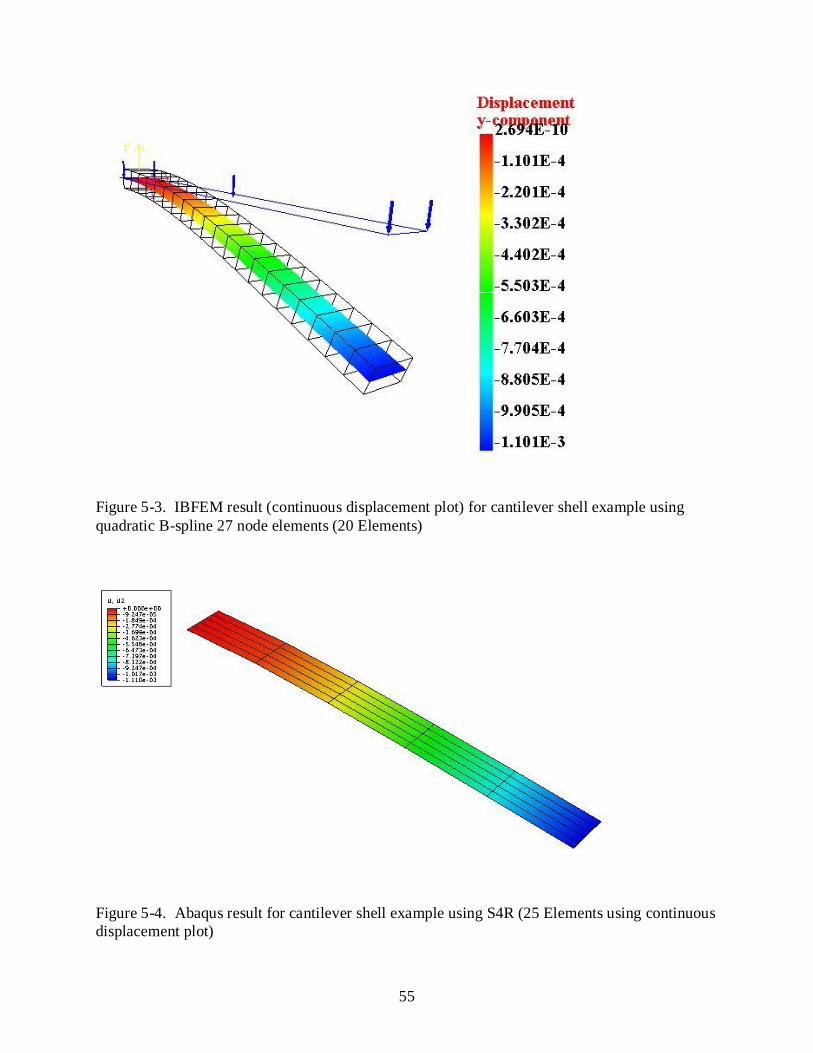
55

Figure 5-3. IBFEM result (continuous displacement plot) for cantilever shell example using quadratic B-spline 27 node elements (20 Elements)

Figure 5-4. Abaqus result for cantilever shell example using S4R (25 Elements using continuous displacement plot)

56

Figure 5-5. ProMechanica result (continuous displacement plot) for cantilever shell example using shell type model for analysis (unknown mesh/element type)

Table 5-1. Cantilever shell: results for vertical displacement at the end of cantilever shell, based on various meshes and element types

Element type Elements Max. Vertical displacement

X 10-3 (m)

IBFEM 64N 5 1.088

10 1.1 20 1.106

IBFEM 27N 5 0.904

10 1.072 20 1.101

Abaqus S4R 25 1.110

100 1.110 400 1.111

ProMechanica – 1.106

57

The results of various elements are listed in the table and are compared to a numerically

converged value of 1.11 mm of displacement at the free end of the cantilever shell. The table

shows that the results of IBFEM shell elements are converging with a much fewer number of

elements when compared to the 4 node iso-parametric reduced integration elements suggested by

Hughes and Tezduyar (Hughes and Tezduyar, 1981). The element type and number of elements

used by Pro-Mechanica are unknown but the results are presented for comparison with one more

commercial finite element software.

Simply Supported Shell Problem

Figure 5-6. Simply supported shell

A simply supported shell is subjected to uniformly distributed load of 50 Pa (N/m2) while

the shell is simply supported at its ends. The problem description is shown in figure 5-6.

58

Figure 5-7. IBFEM result (continuous displacement plot) for simply supported shell example using cubic B-spline 64 node elements (10 Elements)

Figure 5-8. IBFEM result (continuous displacement plot) for square plate example using quadratic B-spline 27 node elements (40 Elements)

59

Figure 5-9. Abaqus result for simply supported shell example using shell type model for analysis S4R (900 Elements using continuous displacement plot)

Figure 5-10. ProMechanica result (continuous displacement plot) for simply supported shell example using shell type model for analysis (unknown mesh/element type)

60

Table 5-2. Simply supported shell: results for vertical displacement at the middle of the shell, based on various meshes and element types

Element type Elements Max. Vertical displacement X 10-4 (m)

IBFEM 64N 5 1.175 10 1.187

20 1.187

IBFEM 27N 10 1.133 20 1.182 40 1.187

S4R 100 1.155 400 1.169

900 1.172 ProMechanica - 1.174

The results of various elements are listed in the table and are compared to a numerically

converged value of 0.1187 mm of displacement at the mid-length of the simply supported shell.

The table shows that the results of IBFEM shell elements are converging with a much fewer

number of elements when compared to the 4 node iso-parametric reduced integration elements

suggested by Hughes and Tezduyar (Hughes and Tezduyar, 1981).

Centrally Loaded Square Clamped Plate in Bending

A square plate as shown in the figure 5-11 is loaded centrally by a uniform load of 100 psi.

The material used is structural steel. The nature of the element behavior, convergence studies,

comparison of results with existing FEM techniques, result plots are presented below. The

problem description is shown in figure 5-11. The elements used are 64-node cubic B-spline

elements and 27-node quadratic B-spline elements.

61

Figure 5-11. Centrally loaded square plate

Figure 5-12. IBFEM result (continuous displacement plot) for square plate example using cubic B-spline 64 node elements (5 x 5 Mesh) with 0.1% error

62

Figure 5-13. IBFEM result (continuous displacement plot) for square plate example using quadratic B-spline 27 node elements (40 x 40 Mesh) with 0.1% error

Figure 5-14. Abaqus result for square plate example using S4R (10 x 10 Mesh) with 0% error (continuous displacement plot)

63

Table 5-3. Square plate: results for vertical displacement at the middle of the square plate, based on various meshes and element types

Element type Mesh Max.Vertical displacement X 10-3 (in)

Error compared to 4.055 X 10-3 in

IBFEM 64N 2 x 2 3.562 –12.2% 5 × 5 4.051 –0.1% 10 × 10 4.055 0.0%

IBFEM 27N 10 x 10 3.966 –2.2% 20 × 20 4.043 –0.3% 40 × 40 4.059 0.1%

Abaqus S4R 5 × 5 3.703 –8.7% 10 × 10 4.054 –0.0% 20 x 20 4.055 0.0%

The results of various elements are listed in the table and are compared to a numerically

converged value of 4.055 x 10-3 inch of vertical displacement at the middle of the square plate.

The table shows that the results of IBFEM shell elements are converging with a much fewer

number of elements when compared to the 4 node iso-parametric reduced integration elements

suggested by Hughes and Tezduyar (Hughes and Tezduyar, 1981).

Obstacle Course Benchmark Problems

The shell obstacle course comprises of three problems, the barrel vault roof, pinched

hemisphere and pinched cylinder. Relevance of these problems in the shell analysis is discussed

extensively in the literature by Belytschko (Belytschko, 1986).

Barrel Vault Roof Problem

The dimensions of the structure for this problem are shown in the Figure 5-1. The Barrel

vault roof is subjected to a gravity load. The ends are fixed to a diaphragm while the side edges

are free. Using symmetry, only one-fourth of the structure has been modeled and meshed. The

geometric dimensions, material properties, loads and constraints are shown in the figure 5-15.

64

The thickness of the shell is 3 inch. The converged numerical solution: vertical displacement at

mid-side of the free edge is 3.59 inch (Ashwell and Gallagher, 1976).

Figure 5-15. Barrel vault roof

The elements used are 64-node cubic B-spline elements and 27-node quadratic B-spline

elements and the results are compared with Abaqus 8-node and 9-node iso-parametric shell

elements.

65

Figure 5-16. IBFEM result (continuous displacement plot) for barrel vault roof example using cubic B-spline 64 node elements (4 x 4 Mesh) with 0.1% error

Figure 5-17. IBFEM result (continuous displacement plot) for barrel vault roof example using quadratic B-spline 27 node elements (9 x 9 Mesh) with 0% error

66

Figure 5-18. Abaqus result (continuous displacement plot) for barrel vault roof example using S8R5 (9 x 9 Mesh) with 0.6% error (other quarter modeled with different CSYS) from the Abaqus benchmark examples

Figure 5-19. ProMechanica result (continuous displacement plot) for barrel vault roof example using shell type model for analysis with 0.9% error (unknown mesh/element type)

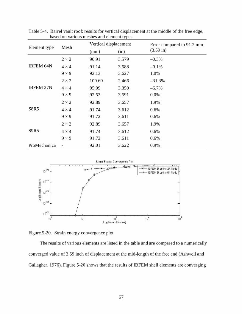
67

Table 5-4. Barrel vault roof: results for vertical displacement at the middle of the free edge, based on various meshes and element types

Element type Mesh Vertical displacement Error compared to 91.2 mm

(3.59 in) (mm) (in)

IBFEM 64N 2 × 2 90.91 3.579 –0.3% 4 × 4 91.14 3.588 –0.1% 9 × 9 92.13 3.627 1.0%

IBFEM 27N 2 × 2 109.60 2.466 –31.3% 4 × 4 95.99 3.350 –6.7% 9 × 9 92.53 3.591 0.0%

S8R5 2 × 2 92.89 3.657 1.9% 4 × 4 91.74 3.612 0.6% 9 × 9 91.72 3.611 0.6%

S9R5 2 × 2 92.89 3.657 1.9% 4 × 4 91.74 3.612 0.6% 9 × 9 91.72 3.611 0.6%

ProMechanica - 92.01 3.622 0.9%

Figure 5-20. Strain energy convergence plot

The results of various elements are listed in the table and are compared to a numerically

converged value of 3.59 inch of displacement at the mid-length of the free end (Ashwell and

Gallagher, 1976). Figure 5-20 shows that the results of IBFEM shell elements are converging

68

with a much fewer number of elements when compared to the 8 node and 9-node iso-parametric

reduced integration elements used by Abaqus.

Pinched Hemisphere Problem

In the pinched hemisphere, the equal and opposite concentrated forces are applied in the

anti-podal points of the equator (Abaqus benchmarks manual and NAFEMS benchmarks, 1990),

the bottom circumferential edge of the hemisphere is free. Due to symmetry, only one-fourth of

the structure is modeled and meshed as shown in the figure 5-20. The material properties,

modulus of elasticity, E = 6.825e7, Poisson’s ratio is 0.3. The thickness of the shell is 0.04m.

The converged numerical solution: radial displacement at loaded points is 185 mm and this

quantity is analyzed for convergence (NAFEMS Benchmarks, 1990).

Figure 5-21. Pinched hemisphere

69

Figure 5-22. IBFEM result (continuous displacement plot) for pinched hemisphere example using cubic B-spline 64 node elements (20 x 20 Mesh) with 10.3% error

Figure 5-23. IBFEM result (continuous displacement plot) for pinched hemisphere example using quadratic B-spline 27 node elements (40 x 40 Mesh) with 9.2% error

70

Figure 5-24. Abaqus result (continuous displacement plot) for pinched hemisphere example using S8R5 (8 x 8 Mesh) with 0% error from the Abaqus benchmark examples

Figure 5-25. ProMechanica result (continuous displacement plot) for pinched hemisphere example using shell type model for analysis with 0.1% error (unknown mesh/element type)

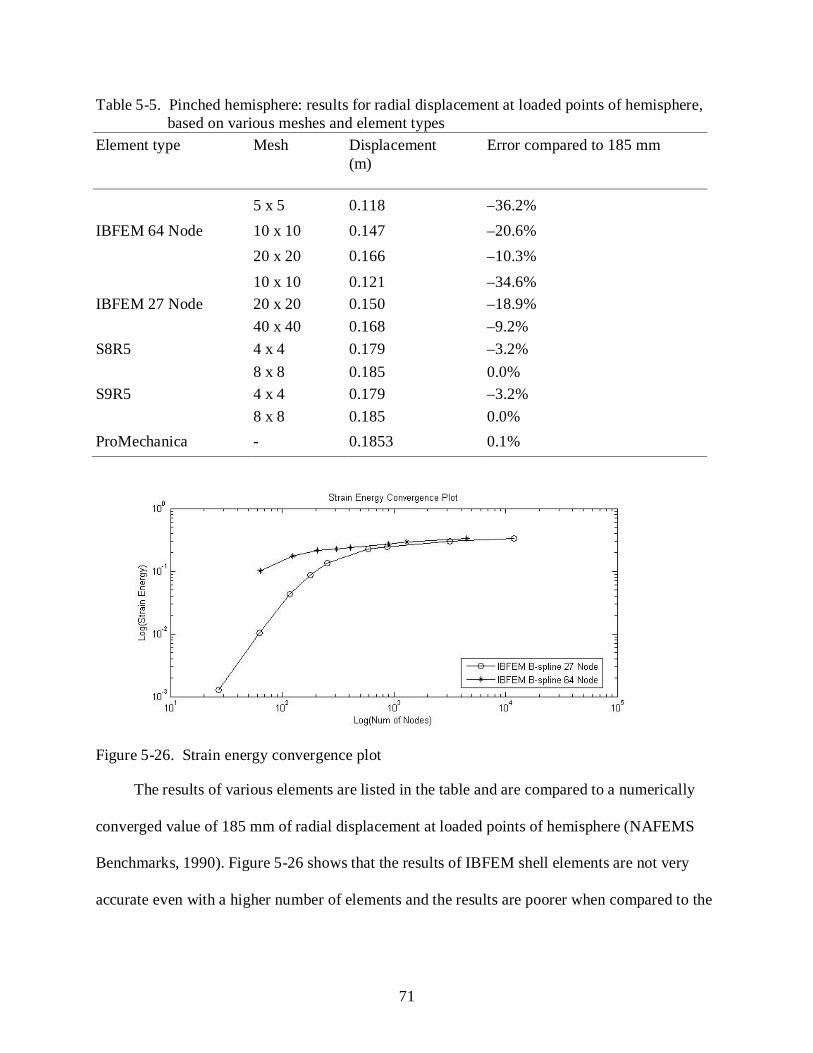
71

Table 5-5. Pinched hemisphere: results for radial displacement at loaded points of hemisphere, based on various meshes and element types

Element type Mesh Displacement (m)

Error compared to 185 mm

IBFEM 64 Node 5 x 5 0.118 –36.2% 10 x 10 0.147 –20.6% 20 x 20 0.166 –10.3%

IBFEM 27 Node 10 x 10 0.121 –34.6% 20 x 20 0.150 –18.9% 40 x 40 0.168 –9.2%

S8R5 4 x 4 0.179 –3.2% 8 x 8 0.185 0.0%

S9R5 4 x 4 0.179 –3.2% 8 x 8 0.185 0.0%

ProMechanica - 0.1853 0.1%

Figure 5-26. Strain energy convergence plot

The results of various elements are listed in the table and are compared to a numerically

converged value of 185 mm of radial displacement at loaded points of hemisphere (NAFEMS

Benchmarks, 1990). Figure 5-26 shows that the results of IBFEM shell elements are not very

accurate even with a higher number of elements and the results are poorer when compared to the

72

8 node and 9-node iso-parametric reduced integration elements used in Abaqus. The reason(s) of

poor results for this example are still unclear.

Pinched Cylinder Problem

The pinched cylinder is subjected to equal and opposite concentrated forces at the mid-

span and the ends of the cylinder are fixed to rigid diaphragm. Due to this boundary condition,

there is a concentrated stress at the point of loading and this causes localized deformation. Due to

symmetry, only one-eighth of the structure is modeled and meshed. The geometric dimensions,

material properties, loads and constraints are shown in the figure 5-25. The converged numerical

solution: radial displacement at loaded points is 1.825 x 10-5in and this quantity is analyzed for

convergence (Lindberg, Olson and Cowper, 1969).

Figure 5-27. Pinched cylinder

The elements used are 64-node cubic B-spline elements and 27-node quadratic B-spline

elements and the results are compared with Abaqus 8-node and 9-node iso-parametric shell

elements.

73

Figure 5-28. IBFEM result (continuous displacement plot) for pinched cylinder example using cubic B-spline 64 node elements (20 x 20 Mesh) with 0.2% error

Figure 5-29. IBFEM result (continuous displacement plot) for pinched cylinder example using quadratic B-spline 27 node elements (20 x 20 Mesh) with 4.9% error

74

Figure 5-30. Abaqus result (continuous displacement plot) for pinched cylinder example using S4R (20 x 30 Mesh) with 0.4% error from the Abaqus benchmark examples

Figure 5-31. ProMechanica result (continuous displacement plot) for pinched cylinder example using shell type model for analysis with 0.4% error (unknown mesh/element type)

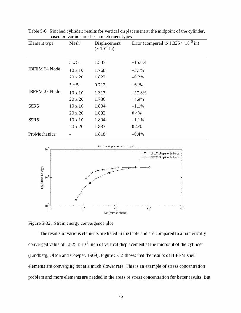
75

Table 5-6. Pinched cylinder: results for vertical displacement at the midpoint of the cylinder, based on various meshes and element types

Element type Mesh Displacement (× 10–5 in)

Error (compared to 1.825 × 10–5 in)

IBFEM 64 Node 5 x 5 1.537 –15.8%

10 x 10 1.768 –3.1% 20 x 20 1.822 –0.2%

IBFEM 27 Node 5 x 5 0.712 –61%

10 x 10 1.317 –27.8% 20 x 20 1.736 –4.9%

S8R5 10 x 10 1.804 –1.1% 20 x 20 1.833 0.4%

S9R5 10 x 10 1.804 –1.1% 20 x 20 1.833 0.4%

ProMechanica - 1.818 –0.4%

Figure 5-32. Strain energy convergence plot

The results of various elements are listed in the table and are compared to a numerically

converged value of 1.825 x 10-5 inch of vertical displacement at the midpoint of the cylinder

(Lindberg, Olson and Cowper, 1969). Figure 5-32 shows that the results of IBFEM shell

elements are converging but at a much slower rate. This is an example of stress concentration

problem and more elements are needed in the areas of stress concentration for better results. But

76

the elements used in this thesis are higher order elements and are computationally expensive

when compared to the 8 node and 9-node iso-parametric reduced integration elements used by

Abaqus. By using adaptive mesh refinement techniques, computational resources can be

concentrated near the location of interest (stress concentration) and can be conserved at all other

locations.

Micro Air Vehicle Wing

The dimensions of the structure for this problem are shown in the figure 5-30. The micro

air vehicle wing is subjected to a traction load. One end is fixed to a diaphragm while the side

edges are free. Due to lack of symmetry, the whole structure has been modeled and meshed. The

geometric dimensions, material properties, loads and constraints are shown in the figure 5-30.

The thickness of the shell is 0.1 inch. The converged numerical solution: vertical displacement at

tip of the free edge is 2.15 inch and this quantity is analyzed for convergence.

Figure 5-33. Micro Air Vehicle Wing

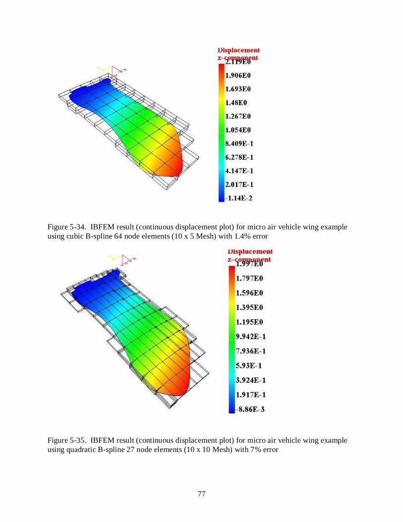
77

Figure 5-34. IBFEM result (continuous displacement plot) for micro air vehicle wing example using cubic B-spline 64 node elements (10 x 5 Mesh) with 1.4% error

Figure 5-35. IBFEM result (continuous displacement plot) for micro air vehicle wing example using quadratic B-spline 27 node elements (10 x 10 Mesh) with 7% error

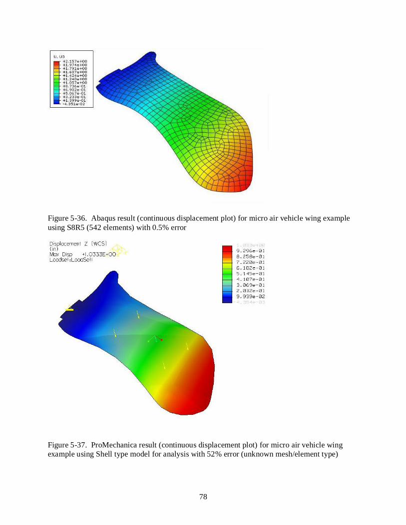
78

Figure 5-36. Abaqus result (continuous displacement plot) for micro air vehicle wing example using S8R5 (542 elements) with 0.5% error

Figure 5-37. ProMechanica result (continuous displacement plot) for micro air vehicle wing example using Shell type model for analysis with 52% error (unknown mesh/element type)

79

The figures show that the results of IBFEM shell elements are consistent with the results of

the 8 node and 9-node iso-parametric reduced integration elements used by Abaqus. For

unknown reasons the results of the shell elements used in Pro Mechnica are poorer.

80

CHAPTER 6 CONCLUSION

Conclusions

In this thesis, shell elements based on uniform B-spline basis defined over a structured grid

are constructed to obtain solutions with continuous gradients throughout the analysis domain.

Implicit boundary finite element method (IBFEM) using B-spline approximation is extended to

shells. Both quadratic and cubic B-spline basis are used for shell analysis. The weak form for

linear elasticity was modified such that essential boundary conditions are imposed properly.

Methods for efficiently and accurately evaluating the terms involved in the modified weak form

were developed.

The primary motivation is the desire to obtain good quality results for shell elements in

finite element analysis by using structured grids and uniform B-spline approximations. Results

obtained using IBFEM shell elements are compared to traditional shell elements used by

commercial FEA applications like Abaqus and Pro-Mechanica. The comparison shows that the

results obtained using IBFEM shell elements converges with fewer elements when compared to

the 4-node, 8-node and 9-node iso-parametric elements suggested by Hughes and Tezduyar

(Hughes and Tezduyar, 1981). The performances of IBFEM shell elements are evaluated and it

passes the obstacle course test except for the pinched hemisphere example. The reason(s) for

slow convergence behavior for this particular example is still unknown. For all other examples,

the IBFEM shell elements studied in this thesis exhibited good convergence behavior.

The advantage of using IBFEM for developing shell elements is the ability to use non-

conforming mesh / grid for the analysis. Generating a uniform structured grid that encloses the

geometry is simpler than generating a conforming mesh because structured grids are independent

of the complexity of the geometry. Also all the elements used in the analysis are regular and

81

undistorted unlike traditional FEM and hence problems associated with distorted elements are

eliminated.

All the techniques presented in this thesis were implemented into a JAVA program.

Several examples were tested for the purpose of validating the methods developed. A few of

those examples are provided in this thesis and it was observed that the methods are capable of

providing solutions that are as good as traditional shell elements.

Scope for Future Work

The IBFEM shell elements developed in this thesis are currently used for analysis of linear

elastic problems only. The IBFEM shell elements can be extended to non-linear analysis like

large elastic deformation, elasto-plastic deformations, and fracture mechanics.

The performance of the IBFEM shell elements can be further improved by incorporating

adaptive mesh refinement. The stress concentrations problems can be analyzed faster with

adaptive mesh refinement. Computational resources can be concentrated near the location of

interest (stress concentration) and can be conserved at all other locations. The shell elements

using IBFEM can also be extended to mixed solid-shell type analysis where thin shells are

attached to solid structures.

82

LIST OF REFERENCES

Abaqus Benchmarks Manual (v6.8)

Ashwell D. G., Gallagher R.H., 1976. Finite Elements for Thin Shells and Curved Members. John Wiley and Sons, London.

Atluri S.N., Kim H.G., Cho J.Y., 1999. Critical assessment of the truly Meshless Local Petrov-Galerkin (MLPG), and Local Boundary Integral Equation (LBIE) methods. Computational Mechanics 24(5) 348–372.

Atluri S.N., Zhu T.L., 2000a. Meshless local Petrov-Galerkin (MLPG) approach for solving problems in elasto-statics. Computational Mechanics 25(2–3) 169–179.

Atluri S.N., Zhu T., 2000b. New concepts in meshless methods. International Journal for Numerical Methods in Engineering 47(1) 537–556.

Babuska I., Banerjee U., Osborn, J.E., 2002. On principles for the selection of shape functions for the Generalized Finite Element Method, Computer Methods in Applied Mechanics and Engineering 191(49–50) 5595–5629

Bathe K.J., Dvorkin E.N., 1985. A four-node plate bending element based on Mindlin-Reissner theory and a mixed interpolation. Int. J. Num. Methods in Eng. 21: 367–383

Batoz J.L., Katili I., 1992. Simple triangular Reissner–Mindlin plate based on incompatible modes and discrete contacts. Int. J. Num. Methods in Eng. 35: 1603–1632

Belytschko T., 1986. A Review of Recent Developments in Plate and Shell Elements. Computational Mechanics-Advances and Trends, AMD vol. 75, ASME, New York.

Belytschko T., Krongauz Y., Fleming M., Organ D., Snm L., Wing K., 1996. Smoothing and accelerated computations in the element free Galerkin method. Journal of Computational and Applied Mathematics. 74(5) 111–126.

Belytschko T., Krongauz Y., Organ D., Fleming M., Krysl P., 1996. Meshless methods: an overview and recent developments. Computer Methods in Applied Mechanics and Engineering 139(1–4) 3–47.

Belytschko T., Lu Y.Y., Gu L., 1994. Element-free Galerkin methods. International Journal for Numerical Methods in Engineering 37(2) 229–256.

Belytschko T., Parimi C., Moes N., Usui S., Sukumar N., 2003. Structured extended finite element methods for solids defined by implicit surfaces. International Journal for Numerical Methods in Engineering 56(4) 609–635.

Boresi A.P., Schmidt R.J., Sidebottom O.M., 1993. Advanced mechanics of materials. John Wiley and Sons Inc. New York.

83

Braess D., 1997. Finite Elements: Theory, Fast Solvers and Applications in Solid Mechanics. Cambridge University Press, Cambridge

Burla R., 2008. Finite element analysis using uniform B-spline approximation and implicit boundary method. Doctoral Dissertation, University of Florida.

Clark B.W., Anderson D.C., 2003a. The penalty boundary method. Finite Elements in Analysis and Design 39(5–6) 387–401.

Clark B.W., Anderson D.C., 2003b. The penalty boundary method for combining meshes and solid models in finite element analysis. Engineering Computations 20(4) 344–365.

Clough R.W., Tocher J. L., 1964. Analysis of thin arch dams by the finite element method.

Cook R.D., Malkus D.S., Plesha M.E., 1989. Concepts and Applications of Finite Element Analysis. John Wiley & Sons Inc., New York.

Cook R.D., Malkus D.S., Plesha M.E., Witt, R.J., 2003. Concepts and Applications of Finite Element Analysis. John Wiley and Sons Inc., New York.

Dolbow J., Belytschko T., 1999. Numerical integration of the Galerkin weak form in meshfree methods. Computational Mechanics 23(3) 219–230.

Duarte C.A., Babuska I., Oden J.T., 2000. Generalized finite element methods for three-dimensional structural mechanics problems. Computers and Structures 77(2) 215–232

Farin G., 2002. Curves and Surfaces for CAGD: A Practical Guide. Morgan Kaufmann Publishers, San Francisco.

Flügge W., 1960. Stresses in Shells, Springer-Verlag, New York, Second.

Flügge W., 1973. Stresses in Shells, Springer-Verlag, New York, Second.

Gingold R.A., Monaghan J.J., 1982. Kernel estimates as a basis for general particle methods in hydrodynamics. Journal of Computational Physics 46 429–53.

Greene. B. E, Strome. D. R and Weikel. R. C., 1961, “Application of the stiffness method to the analysis of shell structures”, Proc. Aviation Conf. Amer. Soc. Mech. Eng., Los Angeles.

Hughes T.J.R., 1981. Finite elements based upon Mindlin plate theory with particular reference to the four-node bilinear iso parametric element. Journal of Applied Mechanics, 48: 587–596

Hughes T.J.R., Cottrell J.A., Bazilevs Y., 2005. Isogeometric analysis: CAD, finite elements, NURBS, exact geometry and mesh refinement. Computer Methods in Applied Mechanics and Engineering 194 (39–41) 4135–4195.

84

Hughes, T. J. R., Taylor R. L., Kanoknukulchai W., 1977. A Simple and Efficient Finite Element for Plate Bending. International Journal for Numerical Methods in Engineering 11(10) 1529–1543.

Höllig K., Reif V., Wipper J., 2001. Weighted extended B-spline approximation of Dirichlet problems. SIAM Journal on Numerical Analysis 39(2) 442–462.

Höllig K., Reif V., 2003. Non uniform web-splines. Computer Aided Geometric Design 20(5) 277–294.

Höllig K., 2003. Finite element methods with B-splines. SIAM, Philadelphia.

Kantorovich L.V., Krylov V.I., 1958. Approximate Methods of Higher Analysis. Interscience, New York.

Krongauz Y., Belytschko T., 1996. Enforcement of essential boundary conditions in meshless approximations using finite elements. Computer Methods in Applied Mechanics and Engineering 131(1–2) 133–145.

Krongauz, Y., Belytschko, T., 1998. EFG approximation with discontinuous derivatives. International Journal for Numerical Methods in Engineering 41(7) 1215–1233.

Krongauz Y., Belytschko T., 1997. Consistent pseudo-derivatives of meshless methods. Computer Methods in Applied Mechanics and Engineering 146(3–4) 371–386.

Krysl P., Belytschko T., 1997. Element-free Galerkin method: convergence of the continuous and discontinuous shape functions. Computer Methods in Applied Mechanics and Engineering 148(3–4) 257–277.

Kumar A.V., Padmanabhan S., Burla R., 2007. Implicit boundary method for finite element analysis using non-conforming mesh or mesh. International Journal for Numerical Methods in Engineering.

Kumar A.V., Lee J., 2006. Step function representation of solid models and application to mesh free engineering analysis. Journal of Mechanical Design. Transactions of the ASME 128(1) 46–56.

Kumar A.V., Lee J.H., Burla R.K., 2005. Implicit solid modeling for mesh free analysis. In: Proceedings of International Design Engineering Technical Conferences & Computers in Engineering IDETC/CIE Long Beach, California.

Lindberg G.M., Olson M.D., Cowper G.R., 1969. New Developments in the Finite Element Analysis of Shells. Quarterly Bulletin of the Division of Mechanical Engineering and the National Aeronautical Establishment, National Research Council of Canada, vol. 4.

Lucy L.B., 1977. A numerical approach to the testing of the fission hypothesis. The Astronomical Journal 82(12) 1013–24.

85

Melenk J.M., Babuska I., 1996. The partition of unity finite element method: Basic theory and applications. Computer Methods in Applied Mechanics and Engineering 139(1–4) 289–314.

Mindlin R.D., 1951. Influence of rotatory inertia and shear on flexural motions of isotropic elastic plates. ASME Journal of Applied Mechanics, Vol 18.

Padmanabhan, S., 2006. Analysis using non-conforming structured grid and implicit boundary method. Doctoral Dissertation, University of Florida.

Rvachev V.L., Shieko T.I., 1995. R-functions in boundary value problems in mechanics. Applied Mechanics Reviews 48(4) 151–188.

Rvachev V.L., Sheiko T.I., Shapiro V., Tsukanov I., 2001. Transfinite interpolation over implicitly defined sets. Computer-Aided Geometric Design 18(3) 195–220.

Shapiro V., 1998. Theory of R-functions and applications: A primer. CPA Technical Report CPA88-3, Cornell Programmable Automation. Sibley School of Mechanical Engineering.

Shapiro V., Tsukanov I., 1999. Meshfree simulation of deforming domains. Computer Aided Design 31(7) 459–471.

Stricklin J.A. et al., 1969. A rapidly converging triangular plate element. AIAA J. 7 180–181

Sukumar N., Moran B., Belytschko T., 1998. Natural element method in solid mechanics. International Journal for Numerical Methods in Engineering 43(5) 839–887.

The Standard NAFEMS Benchmarks., 1990. Test LE3 from NAFEMS publication TNSB. Rev. 3.

Timoshenko S.P., Goodier J.N., 1969. Theory of Elasticity, McGraw Hill, New York.

Timoshenko S.P., Krieger S.W., 1959. Theory of Plates and Shells, 2nd Edition, McGraw Hill, New York

Zienkiewicz O. C., Taylor R. L., 2000. The Finite Element Method for Solid and Structural Mechanics, Butterworth-Heinemann

86

BIOGRAPHICAL SKETCH

Prem Dheepak Salem Periyasamy was born in 1986 and brought up in a city called Salem

in India. He graduated his high school from Sri Rasi Vinayaga (SRV) High School, Rasipuram,

India in 2003. He graduated with a Bachelor of Science in mechanical engineering from

Visveswaraya National Institute of Technology, Nagpur, India in May 2007. He then enrolled in

the Master of Science Program in mechanical and aerospace engineering at the University of

Florida in fall 2007. His areas of interest include application of finite element analysis, numerical

methods, computer-aided design, continuum mechanics, statistics, algorithms and computer

applications in the field of mechanical engineering.