A Computational Framework for Connection Matrices

…toward a computational homological theory of dynamics

ATDD, 2018

A Computational Framework for Connection Matrices

Kelly Spendlove, Rutgers University

• a dynamical system engenders topological data

• local data (e.g. equilibria) and global data (attractors)

• topological data are ordered and measured with algebra

two flavors of algebra: order theory, algebraic topology

data are ordered by dynamics

fx = �rf

data have algebraic invariants (homology)

dynamical musings

Conley-Morse Theory

‘…if such rough equations are to be of use it is necessary to study them in rough terms.’ C. Conley, CBMS Monograph (1978)

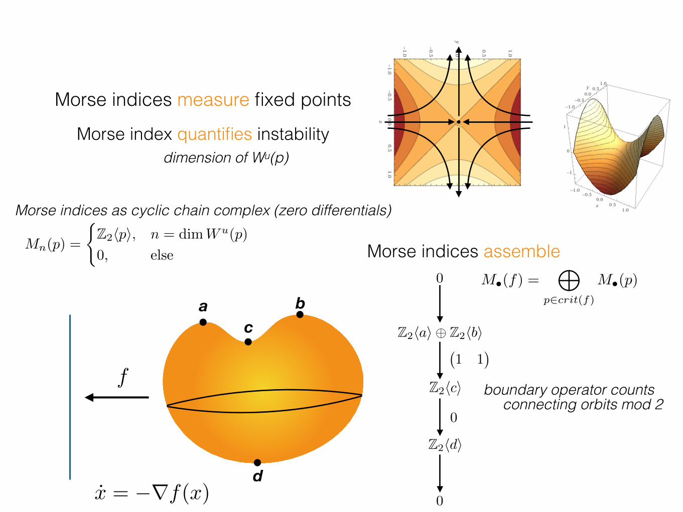
Morse indices measure fixed pointsMorse index quantifies instability

dimension of Wu(p)

Morse indices assemble

a bc

dx = �rf(x)

Z2hai � Z2hbi

Z2hci

Z2hdi

0

0

�1 1

�

0

M•(f) =M

p2crit(f)

M•(p)

Morse indices as cyclic chain complex (zero differentials)

fboundary operator counts

connecting orbits mod 2

Mn(p) =

(Z2hpi, n = dimWu(p)

0, else

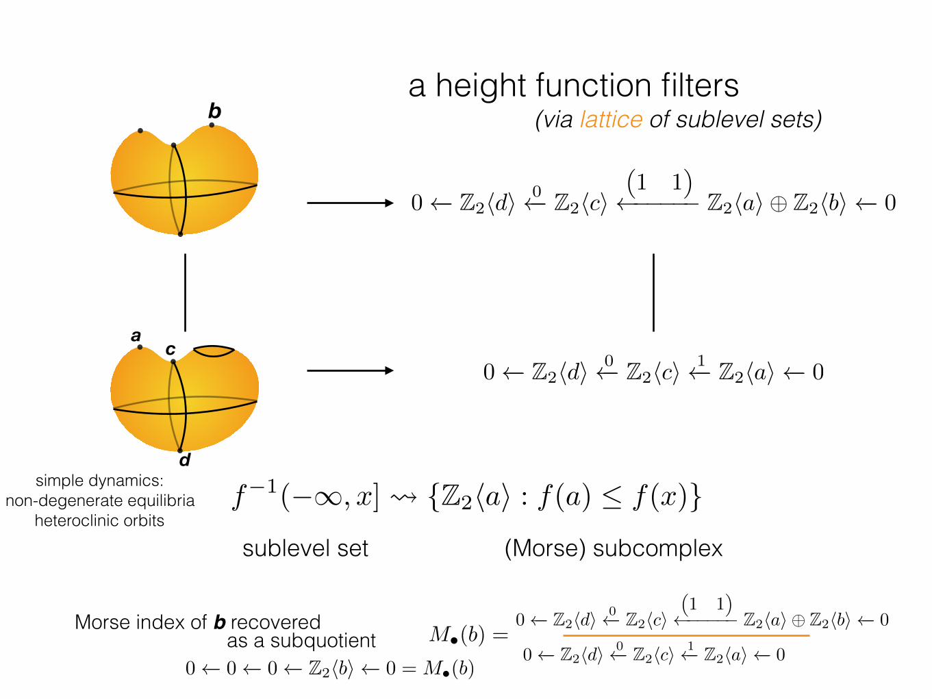
a height function filters

sublevel set (Morse) subcomplex

Morse index of b recovered

b

f�1(�1, x] {Z2hai : f(a) f(x)}simple dynamics: non-degenerate equilibria

heteroclinic orbits

(via lattice of sublevel sets)

c

d

a

0 � Z2hdi0 � Z2hci

1 � Z2hai � 0


⇣1 1

⌘

�� Z2hai � Z2hbi � 0


⇣1 1

⌘

�� Z2hai � Z2hbi � 0


1 � Z2hai � 0M•(b) =as a subquotient

0 � 0 � 0 � Z2hbi � 0 = M•(b)

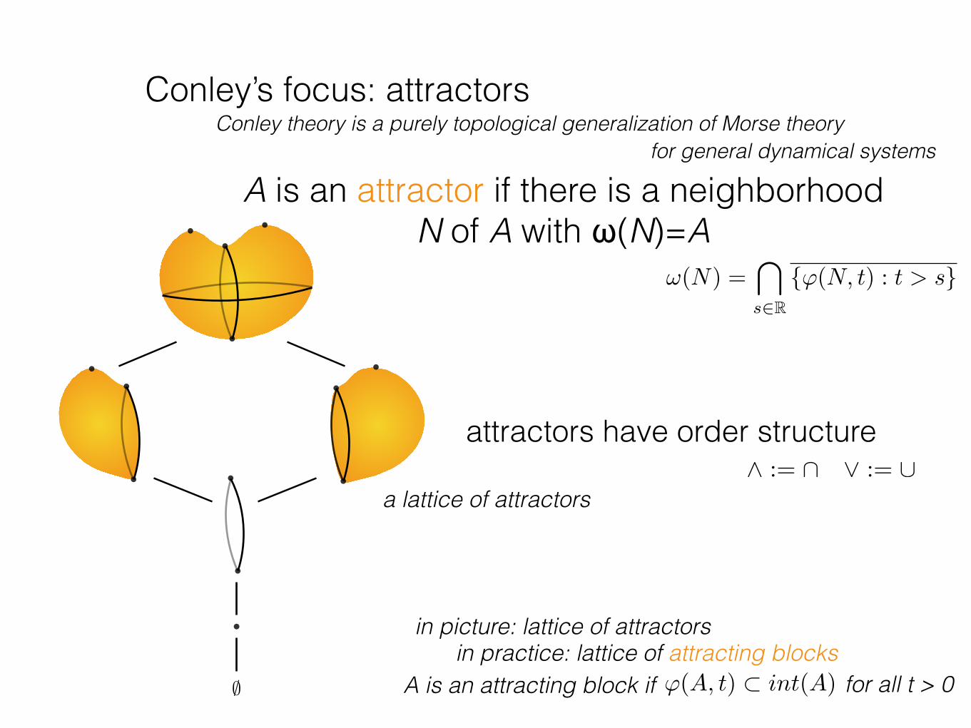
A is an attractor if there is a neighborhood N of A with ω(N)=A

attractors have order structure

;

a lattice of attractors

in practice: lattice of attracting blocksA is an attracting block if '(A, t) ⇢ int(A) for all t > 0

Conley’s focus: attractors

!(N) =\

s2R{'(N, t) : t > s}

Conley theory is a purely topological generalization of Morse theory

in picture: lattice of attractors

for general dynamical systems

^ := \ _ := [

Birkhoff’s theorem

L finite distributive latticethe poset of join irreducible elements of L is

poset the lattice of lower sets is

Fact: O, J are contravariant functorsBirkhoff:

a join-irreducible has a unique predecessor

; O, J are the Birkhoff transforms

(P,)

O(P) := {U ✓ P : if x 2 U and y x then y 2 U}^ := \ _ := [

O(J(L)) ⇠= L J(O(P)) ⇠= P

O J

Pred : J(L) ! L

J(L) := {x 2 L\{0L} : if x = a _ b, then a = x or b = x}

Conley-Morse Homology

associate cyclic complex to isolated invariant sets (Conley index)to generalize Morse homology

Franzosa, Mischaikow, McCord, Reineck… Conley-Morse homology is a homology theory

chain complex of Conley indices

a

b

;

A

B

boundary operator is called the connection matrix

L lattice of attracting blocks

poset P

a

b

of invariant sets

characterized by dynamics at the boundary (local instability)

P J(L)⇠=µ

b Ba A

0 � Z2hai0 � Z2hai

1 � Z2hbi � 0

CH•(b) = H•(B,Pred(B)) B = µ(b)

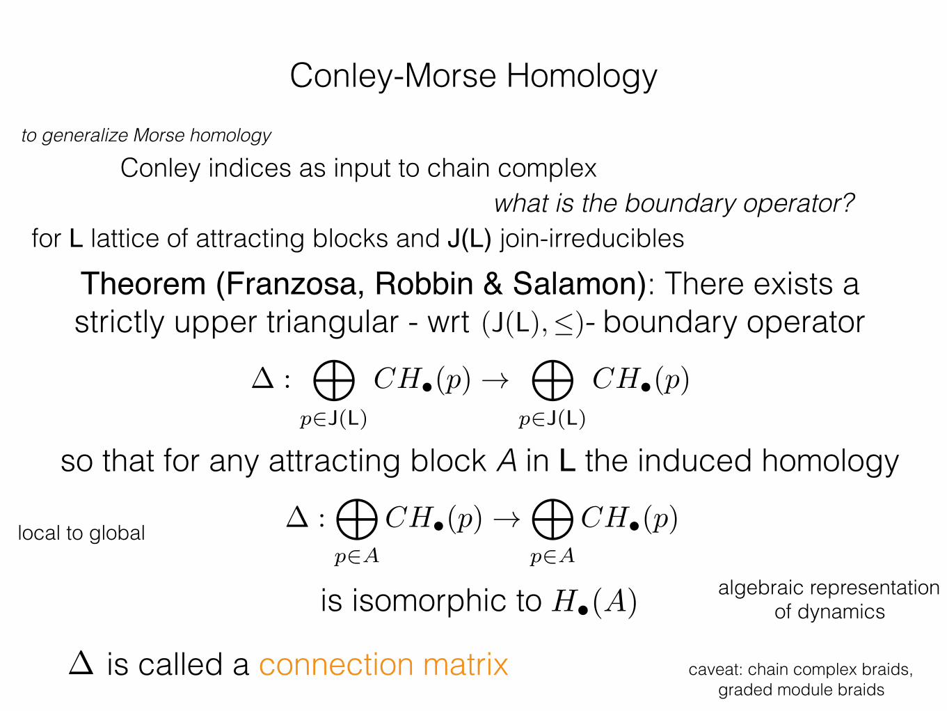
Theorem (Franzosa, Robbin & Salamon): There exists a strictly upper triangular - wrt - boundary operator

Conley indices as input to chain complex

so that for any attracting block A in L the induced homology

� is called a connection matrix

is isomorphic to

caveat: chain complex braids, graded module braids

what is the boundary operator?

local to global

to generalize Morse homology

for L lattice of attracting blocks and J(L) join-irreducibles

(J(L),)

� :M

p2J(L)

CH•(p) !M

p2J(L)

CH•(p)

� :M

p2A

CH•(p) !M

p2A

CH•(p)

Conley-Morse Homology

H•(A)algebraic representation

of dynamics

Categories + Data Structures

‘data! data! data! I can’t make bricks without clay.’ S. Holmes, The Adventure of the Copper Beaches (1892)

Definition (L-filtered chain complex) , L and lattice homomorphism from L to the (modular) lattice of subcomplexes of

L finite, distributive lattice chain complex

L

computational dynamics

Kalies, Mischaikow, van der Vorst, Mrozek, …

homological algebra

(C, @)

Sub(C, @)

(C, @)(C, @)

in practice:

(C, @) is a cell complex with basisL comes from multi-valued map or outer approximation

attracting block subcomplex

{Ca•}a2Lfor the talk we’ll write

Definition (J(L)-graded cell complex)

X, J(L), and a poset morphism from X to J(L)

X cellular complex (Lefschetz, CW)

J(L) poset of join-irreducibles

L finite, distributive lattice

(X, ) face poset

(X, ) (J(L), )

⌫

⌫

Birkhoff transform gives filtered complex

LO(⌫)

Sub(X)

category Ch(L) of L-filtered chain complexes

homotopy category K(L) of L-filtered chain complexes

interpretation of connection matrix for data analysis: ‘small’ representative of homotopy equivalence class

moral: homotopy categories for chain-level data reduction without loss of homological information

the category of L-filtered chain complexes

�(Ca• ) ✓ Ma

•�

0 0

in Ch(L) objects are filtered complexes, morphisms filtered chain maps

C•

Ca• Cb

•

Cc•

M•

Ma• M b

•

M c•

a map is filtered if �

the homotopy category for L-filtered chain complexes

Definition (Filtered homotopy equivalence)

Quadruple such that

isomorphisms in K(L) are filtered homotopy equivalences

{Ma• }a2L{Ca

•}a2L

h h0

are filtered chain maps are filtered homotopies

objects in K(L) are filtered complexes and morphisms are homotopy equivalence classes

�

� �� idC = h@C + @Ch

� � � idM = h0@M + @Mh0( ,�, h, h0)

,� h, h0

Proposition: Over fields, any filtered complex admits a J(L)-splitting

J(L)-splitting for Conley filterings

Definition (Conley filtered)

{Ca•}a2L such that @(Cq

•) ✓ CPred(q)• for q 2 J(L)

(connection matrix for data analysis)

� :M

q2J(L)

H•(Cq, C

Pred(q)) !M

q2J(L)

H•(Cq, C

Pred(q))

this is the classical formula of FranzosaRobbin + Salamon, Harker + Mischaikow + S.

C =M

q2J(L)

Mq where Mq ⇠= Cq/CPred(q) @ :M

q2J(L)

Mq !M

q2J(L)

Mq

A subspace corresponds to a invariant setMq

the (p,q) entry corresponds to connecting orbits@p,q : Mq ! Mp

Framework for Connection Matrices

chain complex

homology

filtered chain complex

Conley-filtered complex

dictionary

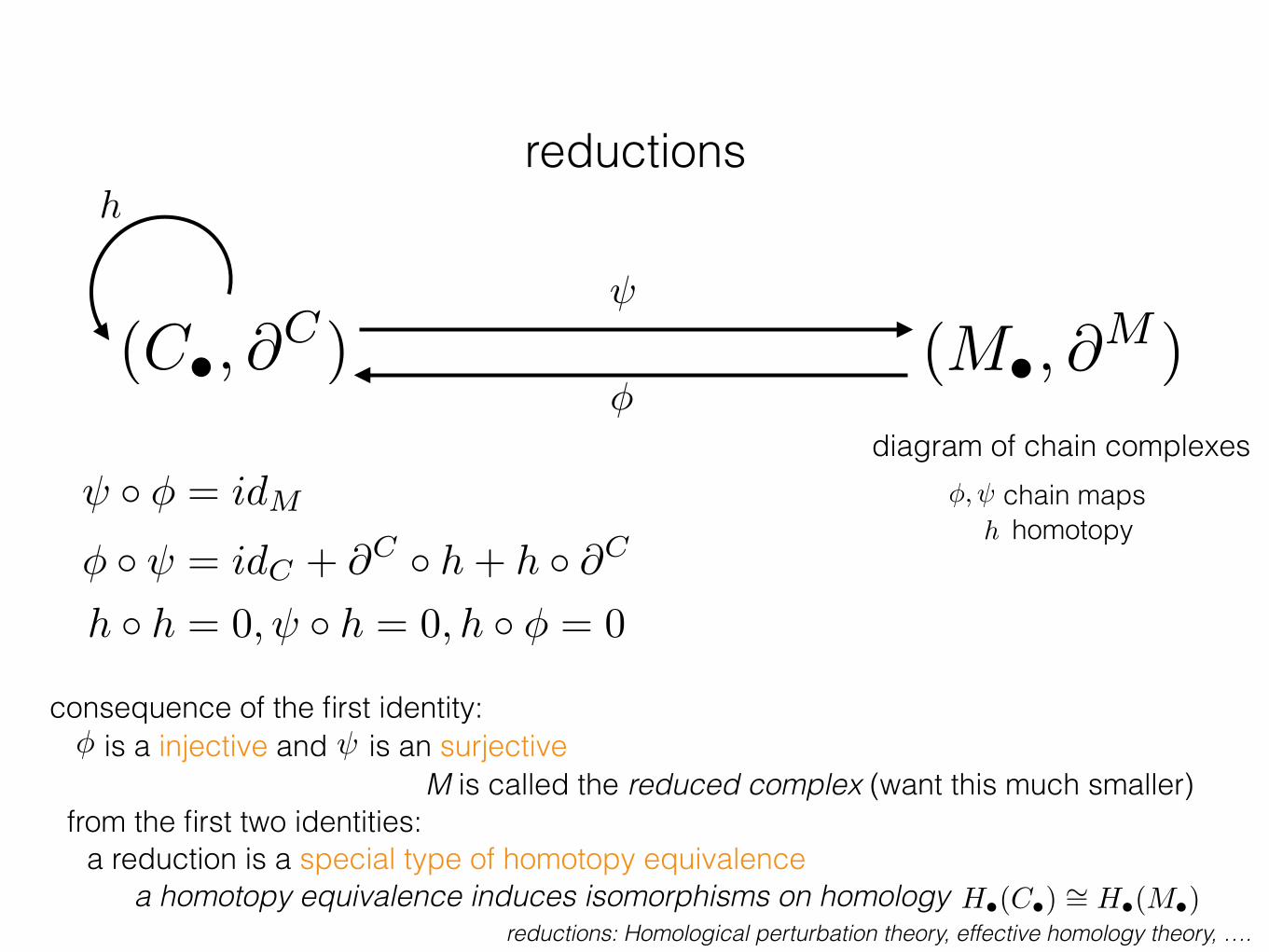
reductions

diagram of chain complexes

is a injective and is an surjectiveM is called the reduced complex (want this much smaller)

reductions: Homological perturbation theory, effective homology theory, ….

a reduction is a special type of homotopy equivalence

consequence of the first identity:

� � = idM

� � = idC + @C � h+ h � @C

h � h = 0, � h = 0, h � � = 0

(M•, @M )(C•, @

C)�

h

from the first two identities:

chain maps�,

h homotopy

�

a homotopy equivalence induces isomorphisms on homology H•(C•) ⇠= H•(M•)

reductions

diagram of chain complexes

H•(C•) ⇠= H•(M•)

using the third set of identities:

� � = idM

� � = idC + @C � h+ h � @C

h � h = 0, � h = 0, h � � = 0

(M•, @M )(C•, @

C)�

h

C• = M• � ker ker is acyclic, i.e. H•(ker ) = 0

… can be done in any category (e.g. filtered) of chain complexes

chain maps�,

h homotopy

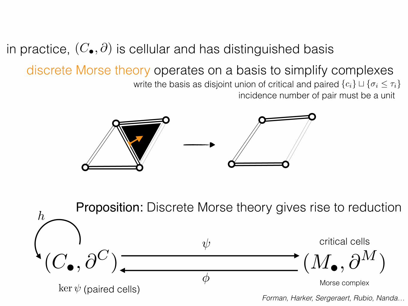
Proposition: Discrete Morse theory gives rise to reduction

discrete Morse theory operates on a basis to simplify complexes

Forman, Harker, Sergeraert, Rubio, Nanda…

(M•, @M )(C•, @

C)�

h

critical cells

incidence number of pair must be a unitwrite the basis as disjoint union of critical and paired {ci} t {�i ⌧i}

Morse complexker (paired cells)

in practice, is cellular and has distinguished basis(C•, @)

tower of reductions

Iterated discrete Morse theory leads to tower of reductions

Proposition: After a finite number of applications of discrete Morse theory the tower stabilizes with @Mn

= 0

Corollary: Homology may be computed with discrete Morse theory

C•

h

M0• . . . Mn

•

h0

�0

0

�1

1 n

�n

@Mn

= 0 =) Mn• = H•(M

n)

(over a field)

Nanda, Dlotko + Wagner, Harker + Mischaikow + S.

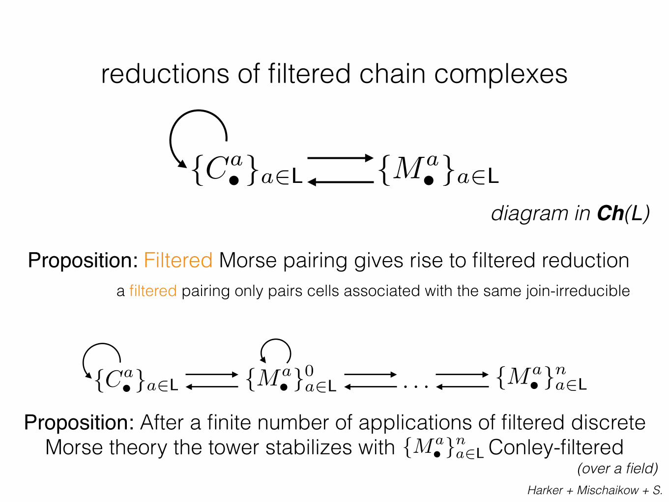
reductions of filtered chain complexes

diagram in Ch(L)

Proposition: Filtered Morse pairing gives rise to filtered reduction a filtered pairing only pairs cells associated with the same join-irreducible

Proposition: After a finite number of applications of filtered discrete Morse theory the tower stabilizes with Conley-filtered{Ma

• }na2L

{Ma• }a2L{Ca

•}a2L

{Ma• }na2L{Ma

• }0a2L{Ca•}a2L . . .

(over a field)Harker + Mischaikow + S.

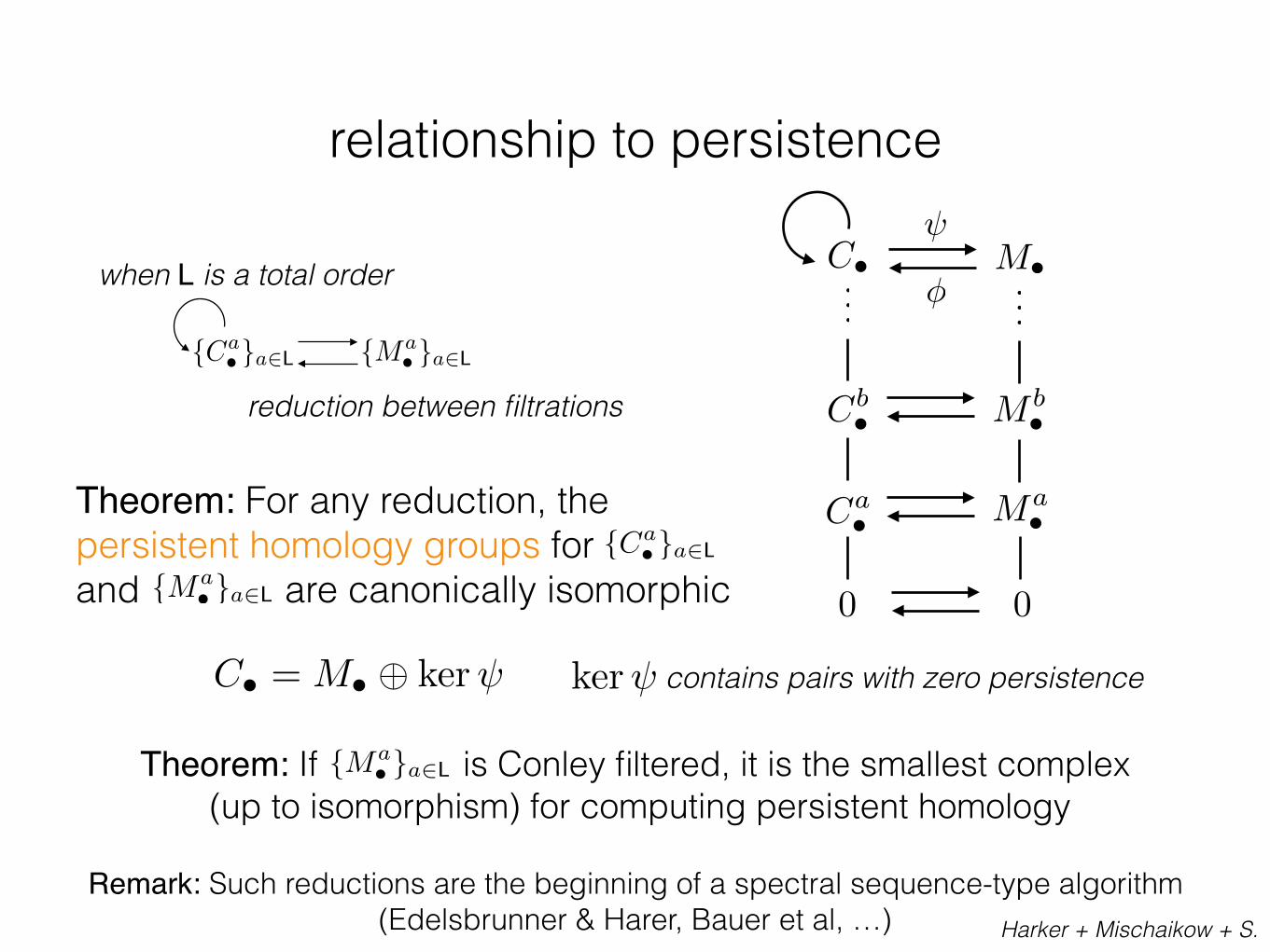
when L is a total order

Remark: Such reductions are the beginning of a spectral sequence-type algorithm (Edelsbrunner & Harer, Bauer et al, …)

relationship to persistence

reduction between filtrations

C• = M• � ker contains pairs with zero persistenceker

{Ma• }a2L{Ca

•}a2L

C•...

M•...

�

Ca•

0

Cb• M b

•

Ma•

0

Theorem: For any reduction, the persistent homology groups for and are canonically isomorphic{Ma

• }a2L

{Ca•}a2L

Theorem: If is Conley filtered, it is the smallest complex (up to isomorphism) for computing persistent homology

{Ma• }a2L

Harker + Mischaikow + S.

‘…it is the author’s belief that in its present form the connection matrix can be applied to many interesting problems by individuals with little or no training in algebraic topology.’

K. Mischaikow, Conley’s Connection Matrix (1987)

computational Conley homology

application + implementation + pedagogy

u0 u1 u2

van den Berg, Ghrist, van der Vorst, Inventiones Math. 2003

u0

u1

Braided equilibrium solutions to parabolic PDE with periodic boundary conditions

Solutions flow across boundary edges from lighter colored tiles to darker

Lattice filtered cubical complex in R2

Fact: Nontrivial Conley indices imply existence of solutions to PDE

Fact: Nonzero entry in connection matrix between adjacent elements proves existence of connecting orbit

Morse theory on braids

dynamics topological data

u0

u1

reduced complex

reduction

index of J(L) : count of cells in the fiber for each dim.data format at a node:

everything but nodes 0,3,6 have trivial Conley indexwhite nodes are trivial indices (no cells)

0:(4,4,1)

1:(2,3,1)

2:(6,10,4)

3:(4,4,1)

4:(2,3,1)

5:(6,10,4)

6:(0,2,1)

7:(4,8,4)

8:(1,2,1)

9:(1,2,1)

10:(4,8,4)

11:(1,2,1)

12:(1,2,1)

(J(L),)(X,)⌫

implementation I

filtered

M•

data reduction…

…without information reduction

0 0 1 0 0 10 0 0

6 node indexcell dim.

30

630

1

1

00

0

0�M =

6/11/2018 2D_Braids_Example

http://localhost:8888/nbconvert/html/2D_Braids_Example.ipynb?download=false 2/5

In [10]: %%time connection_matrix = ConnectionMatrix(fibration)

CPU times: user 2h 5min 23s, sys: 53.1 s, total: 2h 6min 17s

Wall time: 2h 8min 28s

In [11]: morse_poset = Poset(poset)

DrawFibration(connection_matrix, morse_poset)

Out[11]:

(1L, 0L, 0L, 0L, 0L, 0L, 0L, 0L, 0L, 0L) (1L, 0L, 0L, 0L, 0L, 0L, 0L, 0L, 0L, 0L)

(0L, 1L, 0L, 0L, 0L, 0L, 0L, 0L, 0L, 0L)

(0L, 0L, 1L, 0L, 0L, 0L, 0L, 0L, 0L, 0L)

(0L, 0L, 0L, 1L, 0L, 0L, 0L, 0L, 0L, 0L)

(0L, 0L, 0L, 0L, 1L, 0L, 0L, 0L, 0L, 0L)

(0L, 0L, 0L, 0L, 0L, 1L, 0L, 0L, 0L, 0L)

(0L, 0L, 0L, 0L, 0L, 0L, 1L, 0L, 0L, 0L)

(0L, 0L, 0L, 0L, 0L, 0L, 0L, 1L, 0L, 0L)

(0L, 1L, 0L, 0L, 0L, 0L, 0L, 0L, 0L, 0L)

In [12]: %%time reduced_poset = Poset(InducedSubgraph(TransitiveClosure(poset), lambda v

: v in connection_matrix.count()))

CPU times: user 774 ms, sys: 38.5 ms, total: 813 ms

Wall time: 826 ms

In [13]: %%time df = DrawFibration(connection_matrix, reduced_poset)

CPU times: user 173 µs, sys: 23 µs, total: 196 µs

Wall time: 256 µs

In [14]: with open('cm.gv','w') as outfile: outfile.write(df.graphviz())



In [13]: df

Out[13]:

(1L, 0L, 0L, 0L, 0L, 0L, 0L, 0L, 0L, 0L)

(0L, 0L, 1L, 0L, 0L, 0L, 0L, 0L, 0L, 0L)

(0L, 1L, 0L, 0L, 0L, 0L, 0L, 0L, 0L, 0L)

(0L, 0L, 0L, 1L, 0L, 0L, 0L, 0L, 0L, 0L)

(1L, 0L, 0L, 0L, 0L, 0L, 0L, 0L, 0L, 0L)

(0L, 0L, 0L, 0L, 0L, 1L, 0L, 0L, 0L, 0L)

(0L, 0L, 0L, 0L, 1L, 0L, 0L, 0L, 0L, 0L)

(0L, 1L, 0L, 0L, 0L, 0L, 0L, 0L, 0L, 0L)

(0L, 0L, 0L, 0L, 0L, 0L, 0L, 1L, 0L, 0L)

(0L, 0L, 0L, 0L, 0L, 0L, 1L, 0L, 0L, 0L)

In [ ]: # index = 172 # dpset = InducedPoset(poset, lambda v : v in poset.descendants(index)) # DrawFibration(connection_matrix, dpset)

In [ ]:

restrict poset to nodes with nontrivial index

data can get big filtered cubical complex in R9

implementation II

Conley-Morse Graph

connection matrix

cells109 |J(L)| ⇡ 900

initial filtered cubical complex

organizes global dynamics

Conley index for each node



In [13]: df

Out[13]:

(1L, 0L, 0L, 0L, 0L, 0L, 0L, 0L, 0L, 0L)

(0L, 0L, 1L, 0L, 0L, 0L, 0L, 0L, 0L, 0L)

(0L, 1L, 0L, 0L, 0L, 0L, 0L, 0L, 0L, 0L)

(0L, 0L, 0L, 1L, 0L, 0L, 0L, 0L, 0L, 0L)

(1L, 0L, 0L, 0L, 0L, 0L, 0L, 0L, 0L, 0L)

(0L, 0L, 0L, 0L, 0L, 1L, 0L, 0L, 0L, 0L)

(0L, 0L, 0L, 0L, 1L, 0L, 0L, 0L, 0L, 0L)

(0L, 1L, 0L, 0L, 0L, 0L, 0L, 0L, 0L, 0L)

(0L, 0L, 0L, 0L, 0L, 0L, 0L, 1L, 0L, 0L)

(0L, 0L, 0L, 0L, 0L, 0L, 1L, 0L, 0L, 0L)

In [ ]: # index = 172 # dpset = InducedPoset(poset, lambda v : v in poset.descendants(index)) # DrawFibration(connection_matrix, dpset)

In [ ]:



In [15]: bd = lambda cell : connection_matrix.complex().boundary(cell) #valuation = lambda v : v in connection_matrix.count() C = connection_matrix.complex()

print("Connection Matrix Data") print("======================") for d in range(0,C.dimension()): print(" Boundaries of " + str(d) + "-cells (by cell index):") for c in C(d): if connection_matrix.value(c)!= 910: print(" Cell " + str( c) + ' (valuation ' + str(connection_matrix.value(c)) + ') : ' + str(bd({c

})))

Connection Matrix Data

======================

Boundaries of 0-cells (by cell index):

Cell 0 (valuation 0) : set([])



Cell 3 (valuation 12) : set([0L, 1L])




Cell 5 (valuation 67) : set([4L])










In [ ]: morse_poset = Poset(poset)

DrawFibration(connection_matrix, morse_poset)

In [ ]: # new_dag = [poset.add_edge(u,v) if morse_poset(u) & morse_poset.u, v share children] # for v in poset.vertices(): # for u in poset.vertices(): # if for v in morse_poset.vertices(): if v in connection_matrix.count(): continue for u in morse_poset.vertices(): if u in connection_matrix.count(): continue if len(morse_poset.children(v) & morse_poset.children(u)) > 0: poset.add_edge(v,u)

In [ ]: (coarsen,mapping) = CondensationGraph(poset.vertices(),lambda v: poset.adjacencies(v))

cells109

boundaries can be queried from the data structure

order data chain data

implementation III

9 cells

9 cellschain-level data reduction

without loss of homological information

Conley-Morse Graph

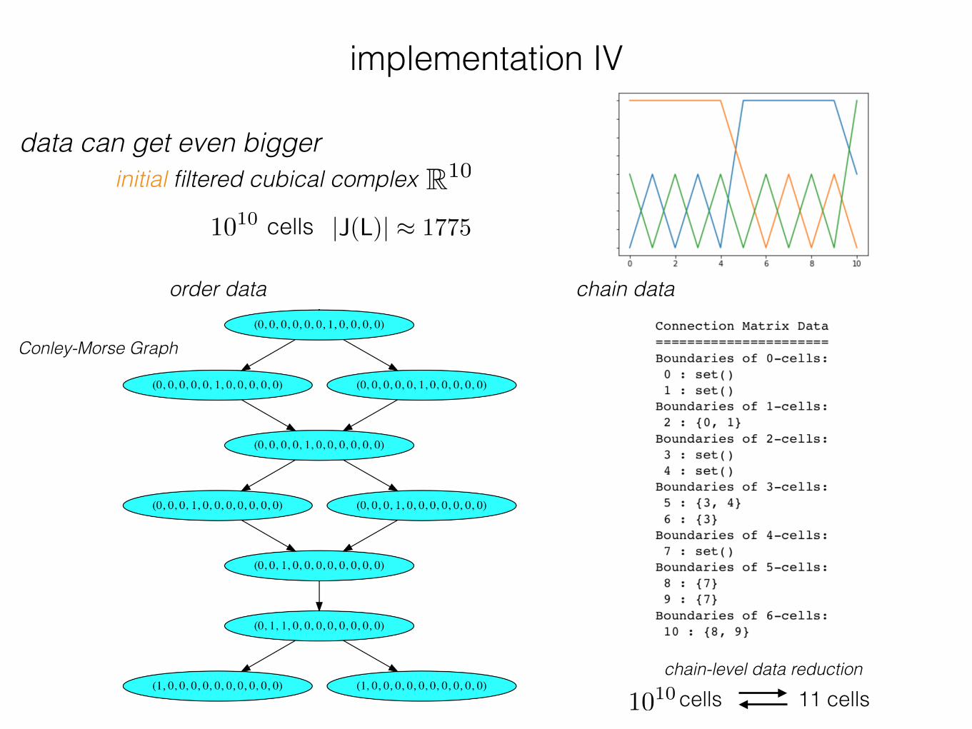
implementation IV

data can get even biggerinitial filtered cubical complex R10

cells1010 |J(L)| ⇡ 1775

cells 11 cellschain-level data reduction

1010

order data chain data

Conley-Morse Graph

Collaborators: S. Harker K. Mischaikow R. van der Vorst

thank you for your attention

A Computational Framework for Connection Matrices

Documents

Transcript of A Computational Framework for Connection Matrices