6/14/2015©Zachary Wartell Visible Surface Detection Copyright 2006, Zachary Wartell at University...

04/18/23©Zachary Wartell

Visible Surface Detection

Copyright 2006, Zachary Wartell at University of North Carolina. All rights reserved.

Revision 1.3

Textbook:Chapter 9


Back-Face Culling

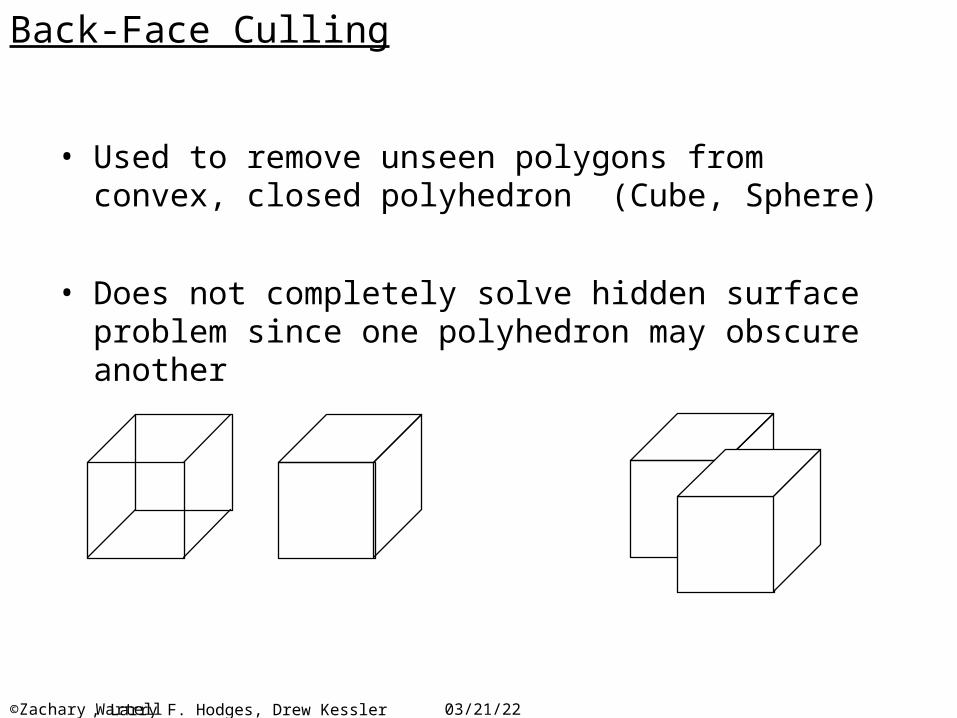
• Used to remove unseen polygons from convex, closed polyhedron (Cube, Sphere)

• Does not completely solve hidden surface problem since one polyhedron may obscure another

, Larry F. Hodges, Drew Kessler


Back Face Culling

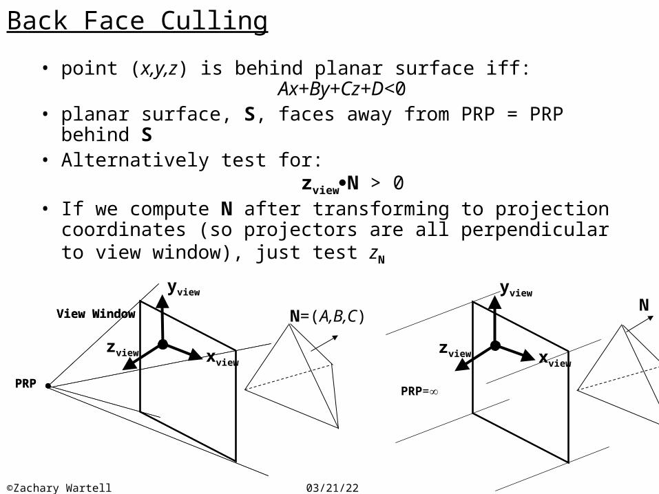
• point (x,y,z) is behind planar surface iff: Ax+By+Cz+D<0

• planar surface, S, faces away from PRP = PRP behind S• Alternatively test for:

zviewN > 0• If we compute N after transforming to projection

coordinates (so projectors are all perpendicular to view window), just test zN

PRP

View Window

PRP

View Window N=(A,B,C)

yview

xview

zview

PRP=

Nyview

xviewzview


Depth-Buffer Method

• Recall Slide:ITCS 4120-3D Viewing.ppt # 51-53, “3D→3D collineation on cube”

http://www.cs.uncc.edu/~zwartell/ITCS%204120-5120/current/Lectures/Wartell/web%20page/ITCS%204120-3D%20Viewing.ppt

http://www.cs.uncc.edu/~zwartell/ITCS%204120-5120/current/Lectures/Wartell/web%20page/ITCS%204120-3D%20Viewing.ppt


Depth-Buffer Algorithm

1. Initialize depth buffer and frame buffer for all pixels (x,y)

depthBuffer(x,y) = 1.0; frameBuffer(x,y)=BackgroundColor

2. Process each polygon face, F, in scene– For each projected pixel, P, at location (x,y) in F,

calculate the depth z– If z < depthBuffer(x,y), compute surface color, C, at

the pixel P, so set: depthBuffer(x,y) = z; frameBuffer(x,y)=C

Note: After all surfaces are processed, depth buffer contains depth for visible surfaces and frame buffer contains corresponding color values for those surfaces


(x1,y1,z1)

(x2,y2,z2)(x3,y3,z3)

(xr,yr,zr)(xl,yl,zl)

(x,y,z)

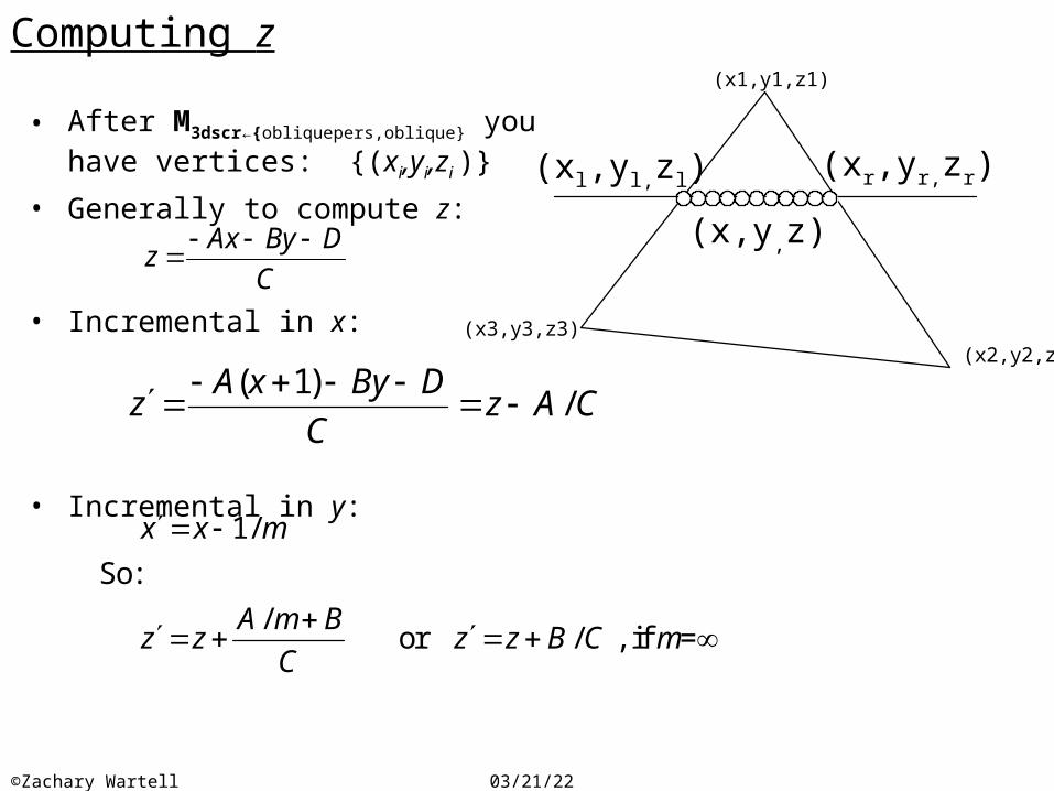
Computing z

• After M3dscr←{obliquepers,oblique} you have vertices: {(xi,yi,zi )}

• Generally to compute z:

• Incremental in x:

• Incremental in y:

Ax By Dz

C

( 1)/

A x By Dz z A C

C

1/

So:

/ or / , if =

x x m

A m Bz z z z B C m

C


A-Buffer Method

• accumulation buffer – buffer accumulates multiple pieces of information for each pixel in addition to depth for transparency or anti-aliasing (high-end movies, etc.). A-buffer element stores:– Depth Field : real-number– Surface Data Field (SDF): stores surface data or pointer

• When Depth >= 0:

-real-number is depth of surface at pixel-SDF is surface color and pixel coverage percentage

depth ≥ 0RGB & Other

Info Pixel44%48%


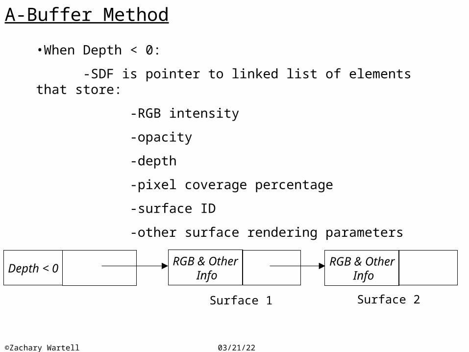
•When Depth < 0:

-SDF is pointer to linked list of elements that store:

-RGB intensity

-opacity

-depth

-pixel coverage percentage

-surface ID

-other surface rendering parameters

A-Buffer Method

Depth < 0RGB & Other

InfoRGB & Other

Info

Surface 1 Surface 2


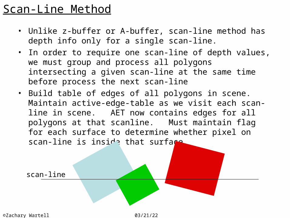
Scan-Line Method

• Unlike z-buffer or A-buffer, scan-line method has depth info only for a single scan-line.

• In order to require one scan-line of depth values, we must group and process all polygons intersecting a given scan-line at the same time before process the next scan-line

• Build table of edges of all polygons in scene. Maintain active-edge-table as we visit each scan-line in scene. AET now contains edges for all polygons at that scanline. Must maintain flag for each surface to determine whether pixel on scan-line is inside that surface.

scan-line


Scan-Line Method Basic Example• Scan Line 1:

– (A,B) to (B,C) only inside S1, so color from S1

– (E,H) to (F,G) only inside S2, so color from S2

• Scan Line 2:– (A,D) to (E,H) only inside S1, so color from S1

– (E,H) to (B,C) inside S1 and S2 , so compute & test depth In this example we color from S1

– (B,C) to (F,G) only inside S2, so color from S2B

A

D

C

G

F

E

H

S1 S2

Scan Line 1

Scan Line 2Scan Line 3


Scan-Line Method Generalization

• This basic approach fails when surfaces cut-through each other or overlap. To generalize we must divide surfaces to eliminate overlaps


Depth-Sorting Method

• Painter’s Algorithm

• Approach:– sorted surfaces by increasing depth

• may require surface splitting– scan-convert surfaces in sorted order (back to

front)

• Use a sequence of sorting steps and tests of increasing computational complexity to handle all possible cases of polygon depth orderings


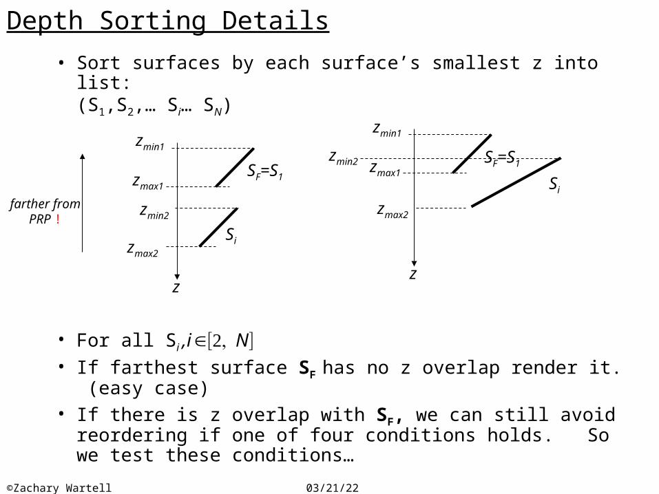
• Sort surfaces by each surface’s smallest z into list: (S1,S2,… Si… SN)

• For all Si ,i N• If farthest surface SF has no z overlap render it.

(easy case)• If there is z overlap with SF, we can still avoid

reordering if one of four conditions holds. So we test these conditions…

Depth Sorting Details

z

SF=S1

Si

zmin2

zmax2

zmin1

zmax1

z

SF=S1

Si

zmin2

zmax2

zmin1

zmax1

farther fromPRP !


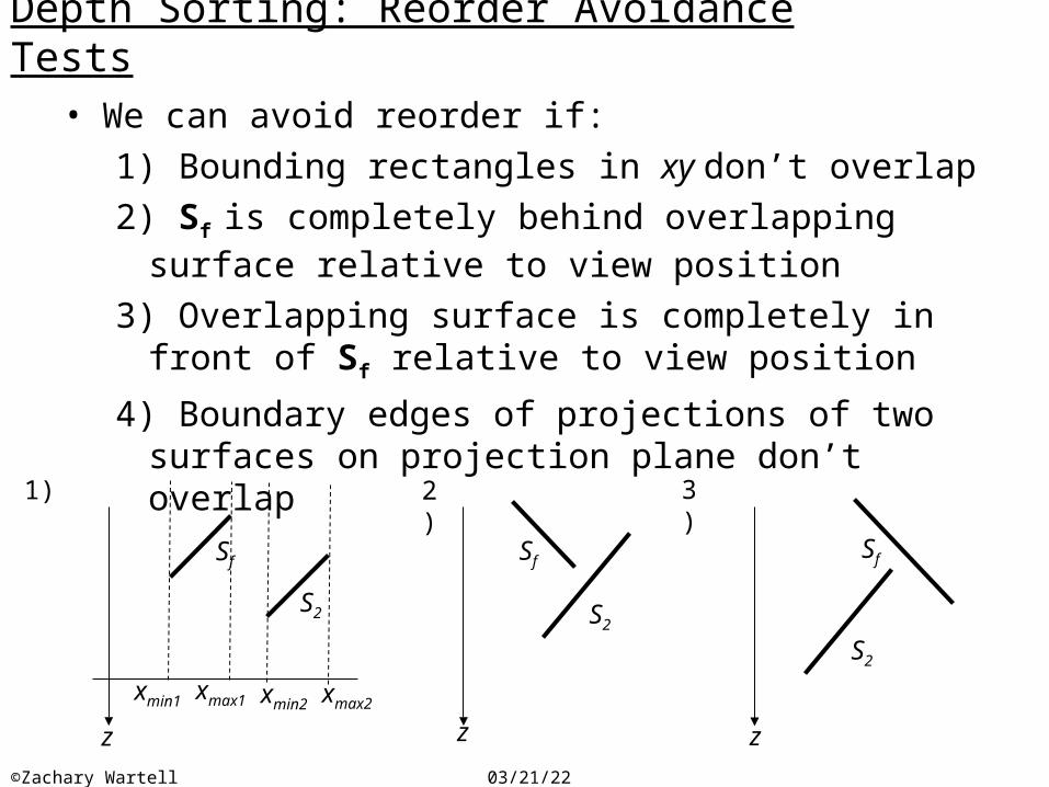
Depth Sorting: Reorder Avoidance Tests

• We can avoid reorder if:1) Bounding rectangles in xy don’t overlap

2) Sf is completely behind overlapping surface relative to view position

3) Overlapping surface is completely in front of Sf relative to view position

4) Boundary edges of projections of two surfaces on projection plane don’t overlap

z

Sf

S2

xmin1 xmax1 xmin2 xmax2

1)

Sf

S2

2) 3)

z z

Sf

S2


Depth Sorting: Reorder Avoidance Tests (cont.)

4) Boundary edges of projections of two surfaces on projection plane don’t overlap. (Knowing that bounding rectangles overlap from (1) doesn’t help. We must compute expensive polygon/polygon intersection).


Depth Sort: Reordering

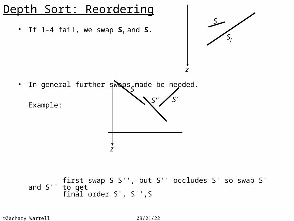
• If 1-4 fail, we swap Sf and S.

• In general further swaps made be needed.

Example:

first swap S S'', but S'' occludes S' so swap S' and S'' to get final order S', S'',S

z

S''

S

S'

z

Sf

S


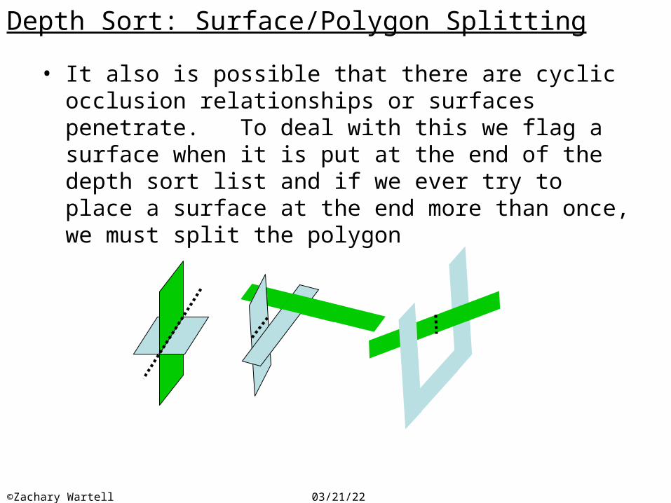
Depth Sort: Surface/Polygon Splitting

• It also is possible that there are cyclic occlusion relationships or surfaces penetrate. To deal with this we flag a surface when it is put at the end of the depth sort list and if we ever try to place a surface at the end more than once, we must split the polygon


BSP-trees

Binary Space Partition is a relatively easy way to sort the polygons relative to the eyepoint

To Build a BSP Tree1. Choose a polygon, T, and compute the equation of the plane it defines.

2. Test all the vertices of all the other polygons to determine if they are in front of, behind, or in the same plane as T. If the plane intersects a polygon, divide the polygon at the plane.

3. Polygons are placed into a binary search tree with T as the root.

4. Call the procedure recursively on the left and right subtree.

Larry F. Hodges, Drew Kessler


BSP-Tree Example

+X -X

C

B

A

D

E

+ZF



Traversing BSP-Tree

• Traverse the BSP tree such that the branch descended first is the side that is away from the eyepoint. This can be determined by substituting the eye point into the plane equation for the polygon at the root.

• When there is no first branch to descend, or that branch has been completed then render the polygon at this node.

• After the current node's polygon has been rendered, descend the branch that is closer to the eyepoint.



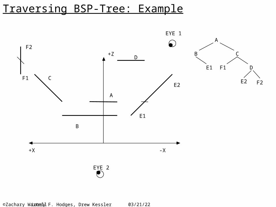
Traversing BSP-Tree: Example

EYE 1

+X -X

C

B

A

D

E1

+ZF2

E2F1

EYE 2

A

C

F1 D

E2 F2

B

E1



Splitting Triangles

If all our polygons are triangles then we always divide a triangle into more triangles when it is intersected by the plane.

• It is possible for the number of triangles to increase exponentially but in practice it is found that the increase may be as small as two fold.

• A heuristic to help minimize the number of fractures is to enter the triangles into the tree in order from largest to smallest.



Area-Subdivision Method

• Recursively subdivide viewplane into quadrants until:– rectangle contains part of 1 projected surface– rectangle contains part of no surface– rectangle is size of pixel


Area-Subdivision Method

• We need tests that can quickly determine tell if current area is part of one surface or if further subdivision is needed.

• Four cases for relation between surface and rectangular area:

surrounding surface

overlapping surface

inside surface

outside surface


Area-Subdivision: Stopping Conditions

• Recursive subdivision can stop when either:1) a rectangle has all surfaces outside2) a rectangle has exactly one inside,

overlapping, or surrounding surface3) a rectangle has one surrounding surface and

the surface occludes all other surfaces in the area

• For efficiency:– compare rectangle to projected surface

bounding rectangle first. Only perform exact interaction test if necessary. If single bounding rect. intersects rectangle, test for exact intersection and color the framebuffer for the intersection of surface & rectangle.


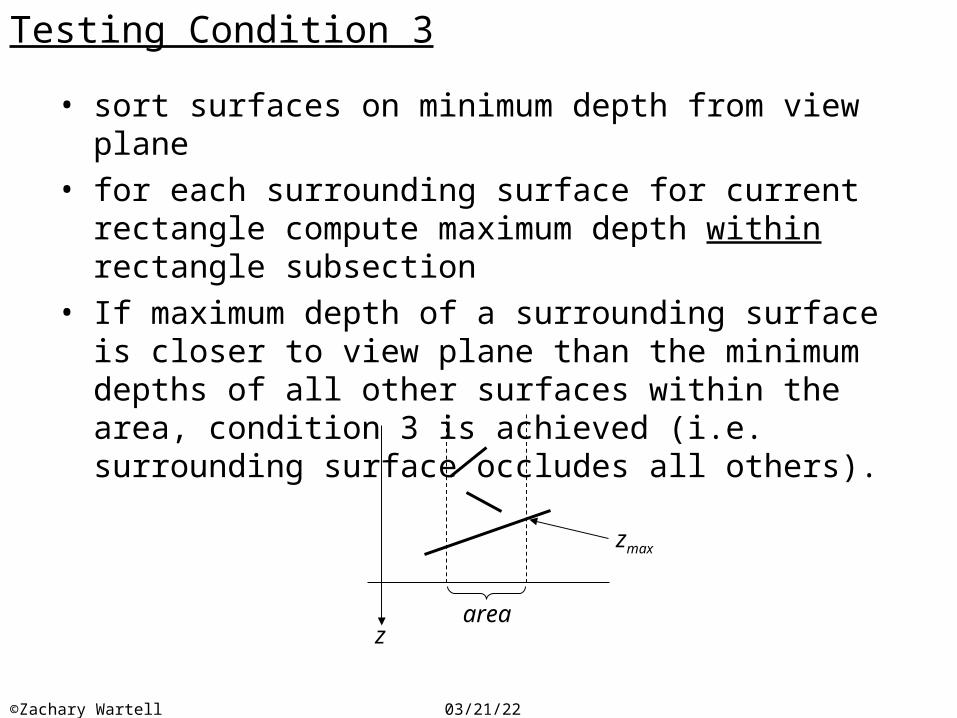
Testing Condition 3

• sort surfaces on minimum depth from view plane• for each surrounding surface for current rectangle

compute maximum depth within rectangle subsection

• If maximum depth of a surrounding surface is closer to view plane than the minimum depths of all other surfaces within the area, condition 3 is achieved (i.e. surrounding surface occludes all others).

zarea

zmax


Condition 3 Test need not be exhaustive

• There are cases that this computation will miss. Rather than performing further more expensive testing, we just subdivide the rectangle (i.e. don’t stop recursion).

• This choice is conservative: we may recurse when we don’t need (to avoid complex geometric computation), but as we continue recursive subdivision we will eventually compute exact answer because in limiting case rectangle is one pixel and in this case we simply calculate depth of each intersecting surface at that single point and set the framebuffer to the nearest surface’s color.


Ray-Casting Method

• based geometric optics method that trace rays of light• “backwards” light path tracing • compare to depth buffer (surfaces to pixels versus pixel to surfaces)• special case of ray-tracing

COP

pixel

view plane


Octrees

• Octree:– partitions 3-space by a regular, recursive subdivision of

3-space into axis-aligned boxes– 3D objects are stored in the octree node that contains

them. Recursively subdivide until each octree node is either empty, a homogeneous volume, or contains single object that’s “easy” to compute visibility (example can use back-face culling alone).

3 2

0 1

4 5

67

0 1 2 3 4 5 6 7

Any of these octants could then be recursively subdivide


Octrees: Rendering

• Given a particular view, the octants can be ordered in view depth order. The order is the same for octants at all levels in the recursive subdivision.

• For general perspective viewing, traverse the octree in back-to-front order and render contents of each node (nearer object’s pixels overwrite farther object’s pixels).

3 2

0 1

4 5

67

view frustum• For parallel projections with

view planes parallel to octant faces, render front-to-backusing a quadtree subdivision of the display window to record when a object has been drawn onto a region of the window.


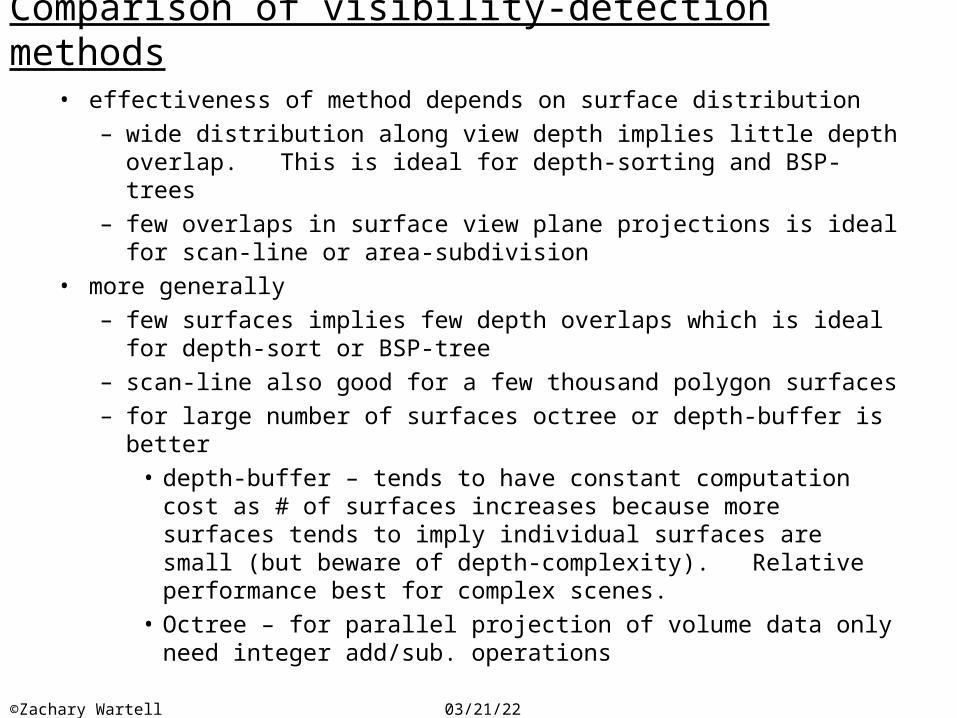
Comparison of visibility-detection methods

• effectiveness of method depends on surface distribution– wide distribution along view depth implies little depth

overlap. This is ideal for depth-sorting and BSP-trees– few overlaps in surface view plane projections is ideal

for scan-line or area-subdivision• more generally

– few surfaces implies few depth overlaps which is ideal for depth-sort or BSP-tree

– scan-line also good for a few thousand polygon surfaces– for large number of surfaces octree or depth-buffer is

better• depth-buffer – tends to have constant computation

cost as # of surfaces increases because more surfaces tends to imply individual surfaces are small (but beware of depth-complexity). Relative performance best for complex scenes.

• Octree – for parallel projection of volume data only need integer add/sub. operations


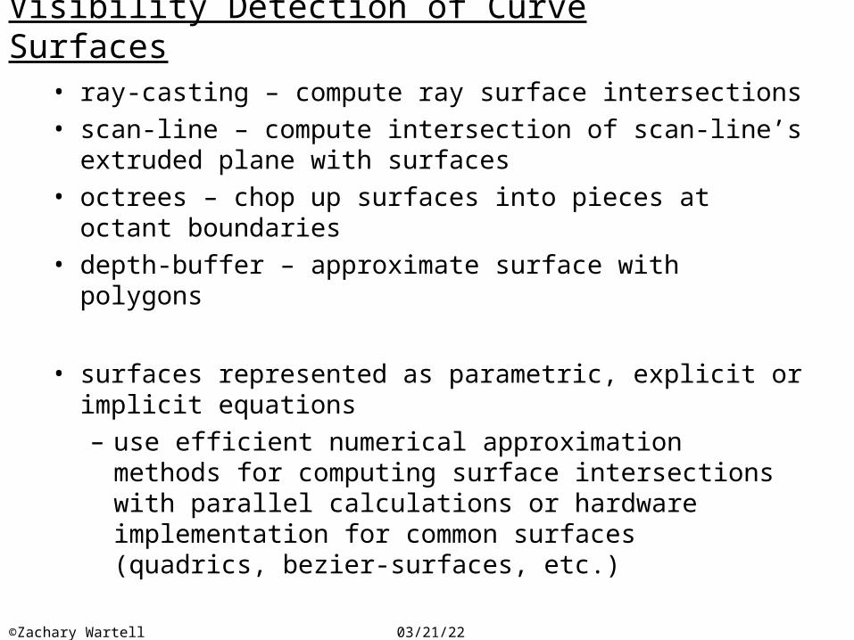
Visibility Detection of Curve Surfaces

• ray-casting – compute ray surface intersections• scan-line – compute intersection of scan-line’s

extruded plane with surfaces• octrees – chop up surfaces into pieces at octant

boundaries• depth-buffer – approximate surface with polygons

• surfaces represented as parametric, explicit or implicit equations– use efficient numerical approximation methods

for computing surface intersections with parallel calculations or hardware implementation for common surfaces (quadrics, bezier-surfaces, etc.)


Surface contour plots

• given some surface representation write it in view coordinate system (z is depth):

y=f(x,z)• plot curves each at fixed z in front-to-back order and

eliminate hidden sections. Increment z by Δz over surfaces visible z range. For each curve, iterate over x coordinate in screen coordinates, compute corresponding y and plot point (x,y). To eliminate hidden surfaces record (ymin,ymax) of plotted points for each x screen coordinate. Only plot point (x,y) if y is outside (ymin,ymax) at x.


Wire-frame visibility methods

• wire-frame rendering of 3D object can be fast (fewer pixels to fill) and can emphasize various 3D features, but it becomes visually ambiguous as to what parts are in front/back of others

• Direct approach requires testing each line segment against each surface. Must work with projected coordinates of segment and surface boundaries. Hidden edges can be removed or drawn with dashes

end points inside & behind

end points inside & infront

end points inside & infront & behind

end points outside & behind at boundary

end points outside & behind & infront

at boundary


Wire-Frame Depth Cueing

• Vary brightness of objects in scene as function of depth:

• Color of point is multiplied by fdepth(d)

• Additionally we could simulate atmospheric effects (smog/haze) where farther pixels are paler in color

max

max min

max min

( )

is distance of point from view position

, application dependent. Often [0.0,1.0] in normalized coordinates

depth

d df d

d d

d

d d


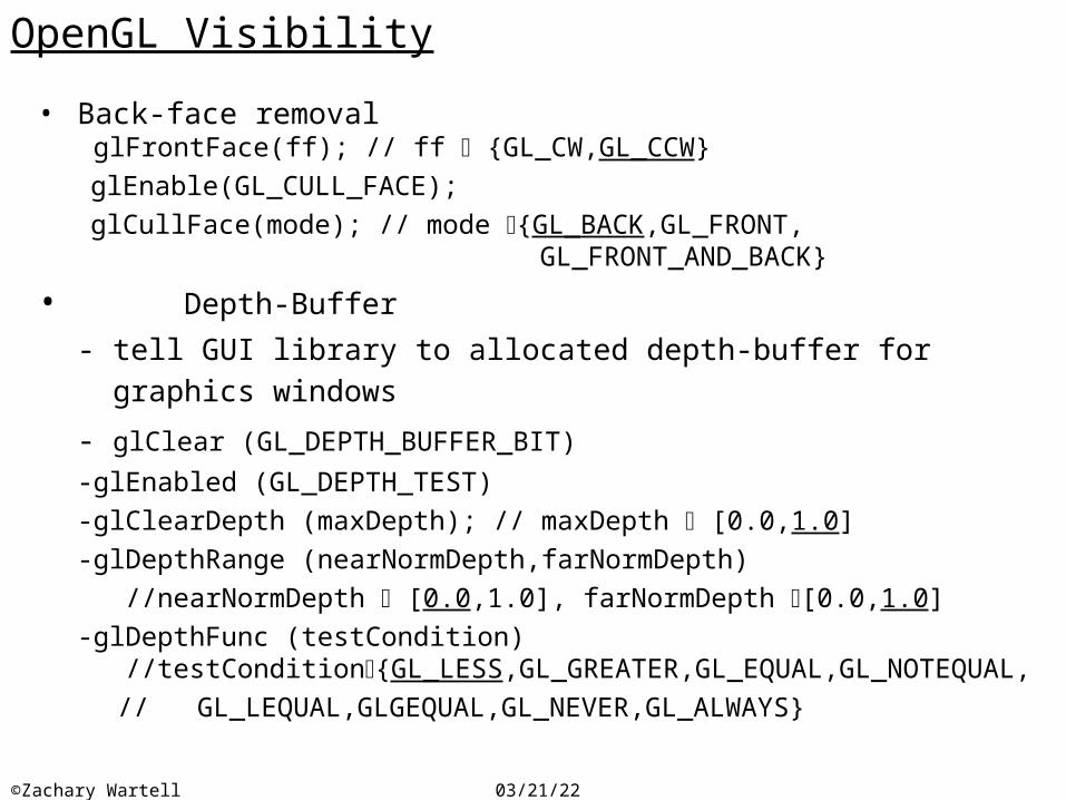
OpenGL Visibility

• Back-face removal glFrontFace(ff); // ff {GL_CW,GL_CCW}glEnable(GL_CULL_FACE);glCullFace(mode); // mode {GL_BACK,GL_FRONT,

GL_FRONT_AND_BACK}

• Depth-Buffer

- tell GUI library to allocated depth-buffer for graphics windows - glClear (GL_DEPTH_BUFFER_BIT)-glEnabled (GL_DEPTH_TEST)-glClearDepth (maxDepth); // maxDepth [0.0,1.0]-glDepthRange (nearNormDepth,farNormDepth) //nearNormDepth [0.0,1.0], farNormDepth [0.0,1.0]-glDepthFunc (testCondition) //testCondition{GL_LESS,GL_GREATER,GL_EQUAL,GL_NOTEQUAL,

// GL_LEQUAL,GLGEQUAL,GL_NEVER,GL_ALWAYS}


OpenGL Visibility (cont.)

• Depth-Buffer– glDepthMask (writeStatus);

// writeStatus {GL_TRUE,GL_FALSE}• use for displaying single animated foreground object over static background

object (disable write when drawing foreground object)• use for approximate transparency (disable write when drawing transparent

surface)

• Wire-frame Surface-Visibility Methods– glPolygonMode(GL_FRONT_AND_BACK,GL_LINE)

• shows polygons as outlines– draw polygon twice. Once as outline using foreground color and once as filled

polygon in background color. To prevent filled polygon pixels from interfering with outline pixels use glPolygonOffset

• Depth-Cueing– glEnable (GL_FOG)– glFogi (GL_FOG_MODE,GL_LINEAR)– glFogf (GL_FOG_START, minDepth)– glFogf (GL_FOG_END, maxDepth)


Revisions

• Revision 1.2– Integrated BSP and Depth Buffer slides from Hodges and Kessler

• Revision 1.3 - typos

6/14/2015©Zachary Wartell Visible Surface Detection Copyright 2006, Zachary Wartell at University...

Documents

Transcript of 6/14/2015©Zachary Wartell Visible Surface Detection Copyright 2006, Zachary Wartell at University...