55:148 Digital Image Processing Chapter 11 3D Vision, Geometry Topics: Basics of projective geometry...
16
55:148 Digital Image Processing Chapter 11 3D Vision, Geometry Topics: Basics of projective geometry Points and hyperplanes in projective space Homography Estimating homography from point correspondence The single perspective camera An overview of single camera calibration Calibration of one camera from the known scene Two cameras, stereopsis The geometry of two cameras. The fundamental matrix Relative motion of the camera; the essential matrix Estimation of a fundamental matrix from image point correspondences Applications of the epipolar geometry in vision Three and more cameras Stereo correspondence algorithms
-
Upload
horace-craig -
Category
Documents
-
view
236 -
download
3
Transcript of 55:148 Digital Image Processing Chapter 11 3D Vision, Geometry Topics: Basics of projective geometry...
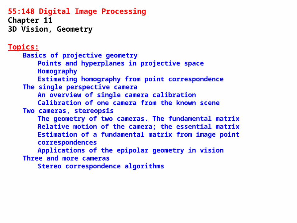
55:148 Digital Image ProcessingChapter 11 3D Vision, Geometry
Topics:Basics of projective geometry
Points and hyperplanes in projective spaceHomographyEstimating homography from point correspondence
The single perspective cameraAn overview of single camera calibrationCalibration of one camera from the known scene
Two cameras, stereopsisThe geometry of two cameras. The fundamental matrixRelative motion of the camera; the essential matrixEstimation of a fundamental matrix from image point correspondencesApplications of the epipolar geometry in vision
Three and more camerasStereo correspondence algorithms
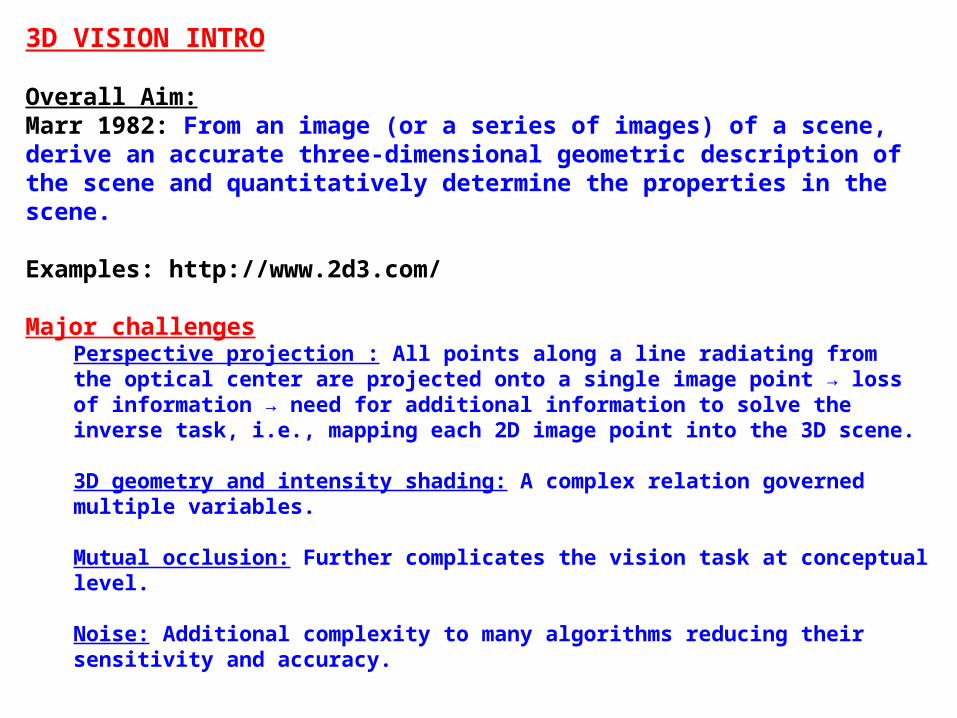
3D VISION INTRO
Overall Aim:Marr 1982: From an image (or a series of images) of a scene, derive an accurate three-dimensional geometric description of the scene and quantitatively determine the properties in the scene.
Examples: http://www.2d3.com/
Major challengesPerspective projection : All points along a line radiating from the optical center are projected onto a single image point → loss of information → need for additional information to solve the inverse task, i.e., mapping each 2D image point into the 3D scene.
3D geometry and intensity shading: A complex relation governed multiple variables.
Mutual occlusion: Further complicates the vision task at conceptual level.
Noise: Additional complexity to many algorithms reducing their sensitivity and accuracy.
3D VISION INTRO
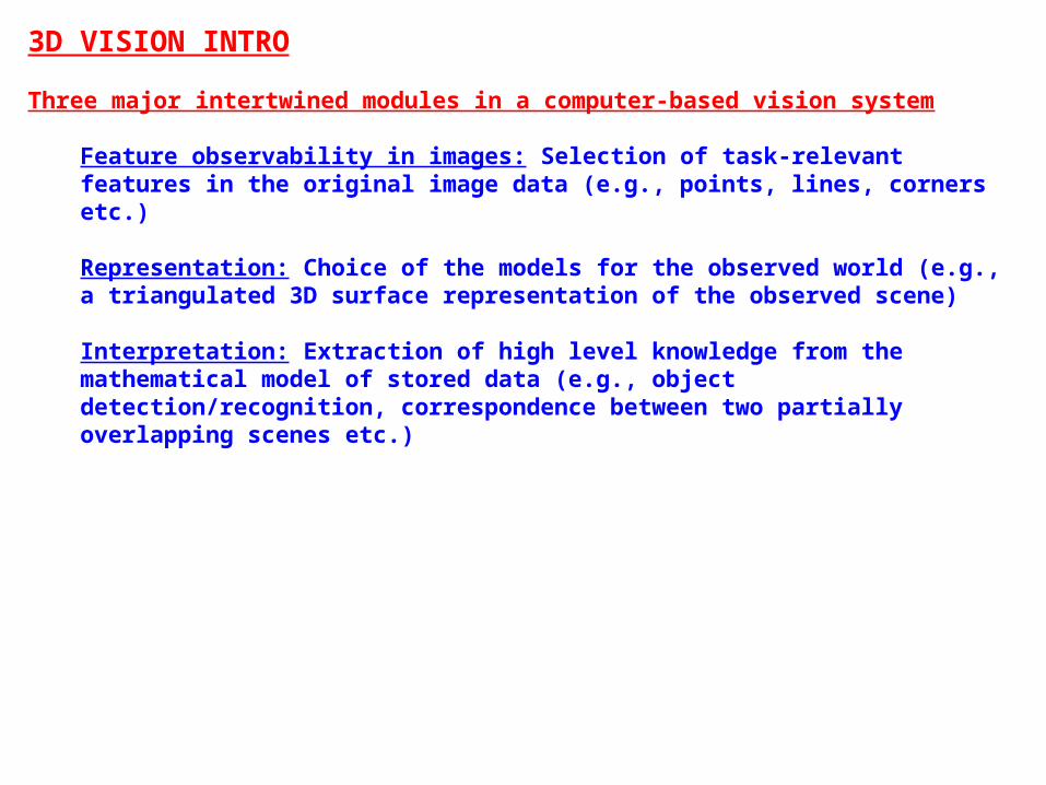
Three major intertwined modules in a computer-based vision system
Feature observability in images: Selection of task-relevant features in the original image data (e.g., points, lines, corners etc.)
Representation: Choice of the models for the observed world (e.g., a triangulated 3D surface representation of the observed scene)
Interpretation: Extraction of high level knowledge from the mathematical model of stored data (e.g., object detection/recognition, correspondence between two partially overlapping scenes etc.)
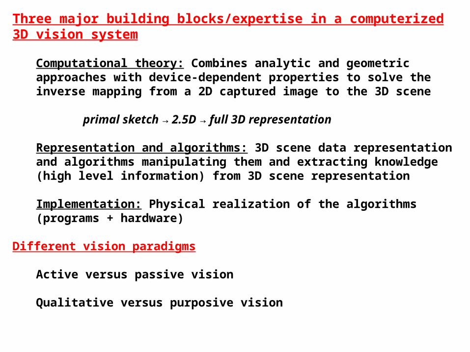
Three major building blocks/expertise in a computerized 3D vision system
Computational theory: Combines analytic and geometric approaches with device-dependent properties to solve the inverse mapping from a 2D captured image to the 3D scene
primal sketch → 2.5D → full 3D representation
Representation and algorithms: 3D scene data representation and algorithms manipulating them and extracting knowledge (high level information) from 3D scene representation
Implementation: Physical realization of the algorithms (programs + hardware)
Different vision paradigms
Active versus passive vision
Qualitative versus purposive vision
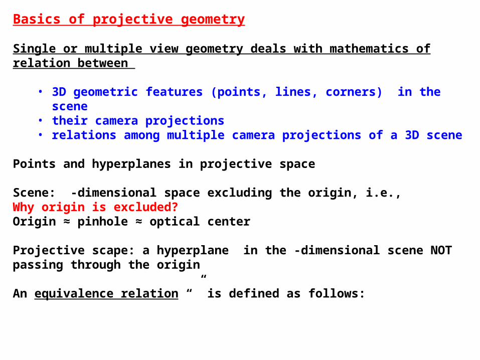
Basics of projective geometry
Single or multiple view geometry deals with mathematics of relation between
• 3D geometric features (points, lines, corners) in the scene• their camera projections• relations among multiple camera projections of a 3D scene
Points and hyperplanes in projective space
Scene: -dimensional space excluding the origin, i.e., Why origin is excluded?Origin ≈ pinhole ≈ optical center
Projective scape: a hyperplane in the -dimensional scene NOT passing through the origin
An equivalence relation “” is defined as follows:
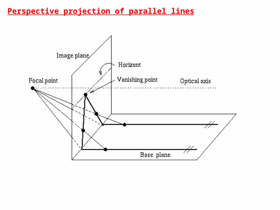
Perspective projection of parallel lines
Homogeneous points
Each equivalent class of the relation “” generates an open line from the origin.
Note that the origin is not included in any of these lines and thus the disjoin property of equivalent classes is satisfied
For each line or equivalent class, exactly one point is projected in the acquired image and is the point where the projective hyperplane intersects the line. These points in the projective space are referred to a homogeneous points.
What is the property of homogenous points?
Homogeneous points are coplanar lying on the projection plane.
For simplicity, let us assume that our projection plane is
Homogeneous points
Note that homogeneous points form the image hyperplane.
Thus, to determine the perspective projection of a scene point, we need to determine corresponding homogeneous point
where .
Note that the points do not have an Euclidean counterpart
• Consider the limiting case that is projectively equivalent to , and assume that .• This corresponds to a point on the projective hyperplane going to infinity in the direction
of the radius vector
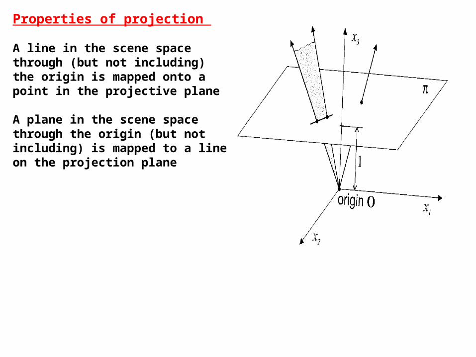
Properties of projection
A line in the scene space through (but not including) the origin is mapped onto a point in the projective plane
A plane in the scene space through the origin (but not including) is mapped to a line on the projection plane
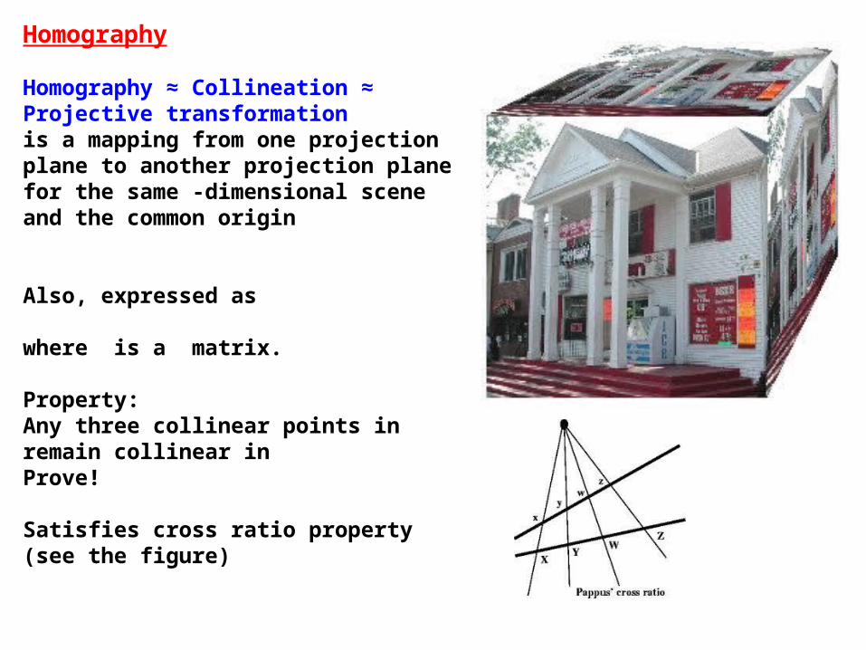
Homography
Homography ≈ Collineation ≈ Projective transformationis a mapping from one projection plane to another projection plane for the same -dimensional scene and the common origin
Also, expressed as
where is a matrix.
Property:Any three collinear points in remain collinear in Prove!
Satisfies cross ratio property (see the figure)
Matrix formulation for Homography
The scale factor and 0; otherwise everything is mapped onto a single point.Eliminating the scale factor , we get
and
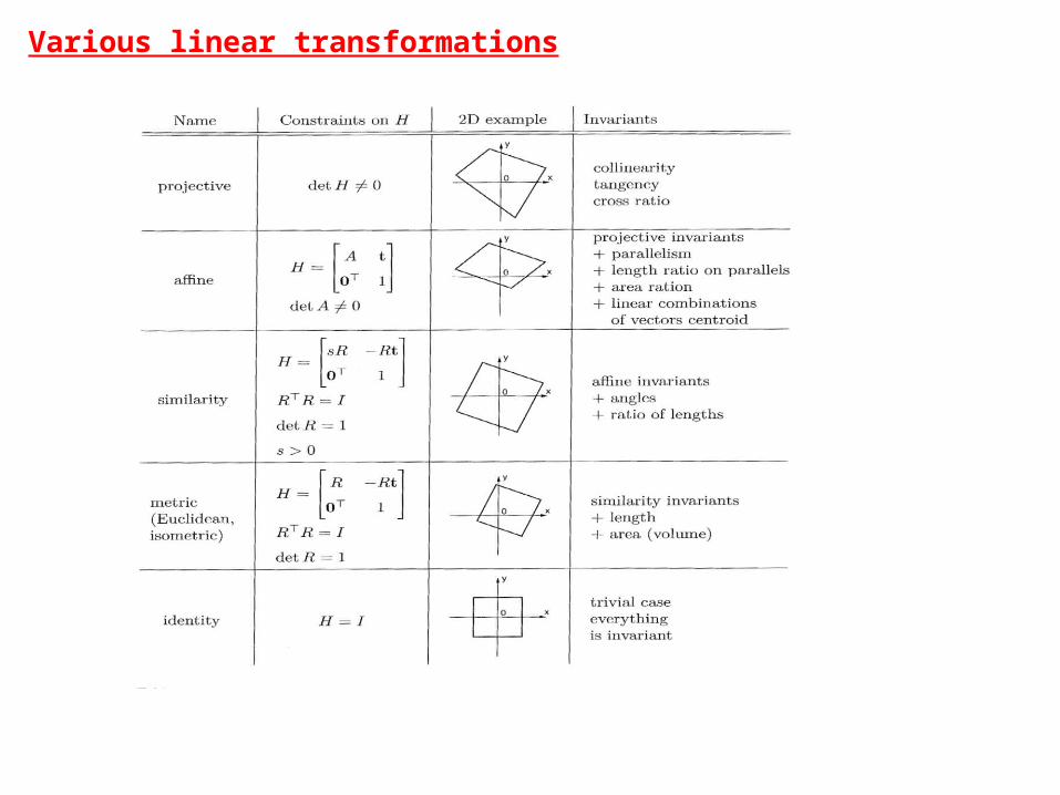
Various linear transformations
Sub groups of homographys
Any homography can be uniquely decomposed as
where , ,
Estimating homography from point correspondence
Given a set of orders pairs of points
To solve the homogeneous system of linear equations
for and .
Number of equations :
Number of unknowns:
Degenerative configuration, i.e., may not be uniquely solved even if and caused when or more points are coplanar
Correspondence of more than sufficient points lead to the notion of optimal fitting reducing the effect of noise
Maximum likelihood estimation
and are identified corresponding points in two different projection planesPrinciple: Find the homography (i.e., the transformation matrix ) that maximizes the likelihood mapping of the points on the first plane to on to the second plane
Model: Ideal points are in the vicinity of the identified points, i.e., there noise in the process of locating the points and
Method to solve the problem
• Determine the ML function using Gaussian model • It contains several multiplicative terms• Take log → multiplications are converted to addition• Remove the minus sign (see the Gaussian expression) • Maximization is converted to a minimization term

Final expression for maximum likelihood estimation