3 Binary Images: Geometric Properties - MIT...

3

Binary Images:Geometric Properties

In this chapter we explore black-and-white (two-valued) images. These areeasier to acquire, store, and process than images in which many brightnesslevels are represented. However, since binary images encode only infor-mation about the silhouette of an object, they are useful only in restrictedsituations. We discuss the conditions that must be satisfied for the success-ful application of binary image-processing techniques. In this chapter weconcentrate on simple geometric properties such as image area, position,and orientation. These quantities are useful in directing the interactionof a mechanical manipulator with a part, for example. Other aspects ofbinary images, such as methods for iterative modification, are explored inthe next chapter.

Since images contain a great deal of information, issues of representa-tion become important. We show that the geometric properties of interestcan be computed from projections of binary images. These projectionsare a great deal easier to store and to process. In much of this chapterwe deal with continuous binary images, where a characteristic function iseither zero or one at every point in the image plane. This makes the pre-sentation simpler; but when we use a digital computer, the image mustbe divided into picture cells. The chapter concludes with a discussion ofdiscrete binary images and ways of exploiting their spatial coherence to

3.1 Binary Images 47

reduce transmission and storage costs, as well as processing time.

3.1 Binary Images

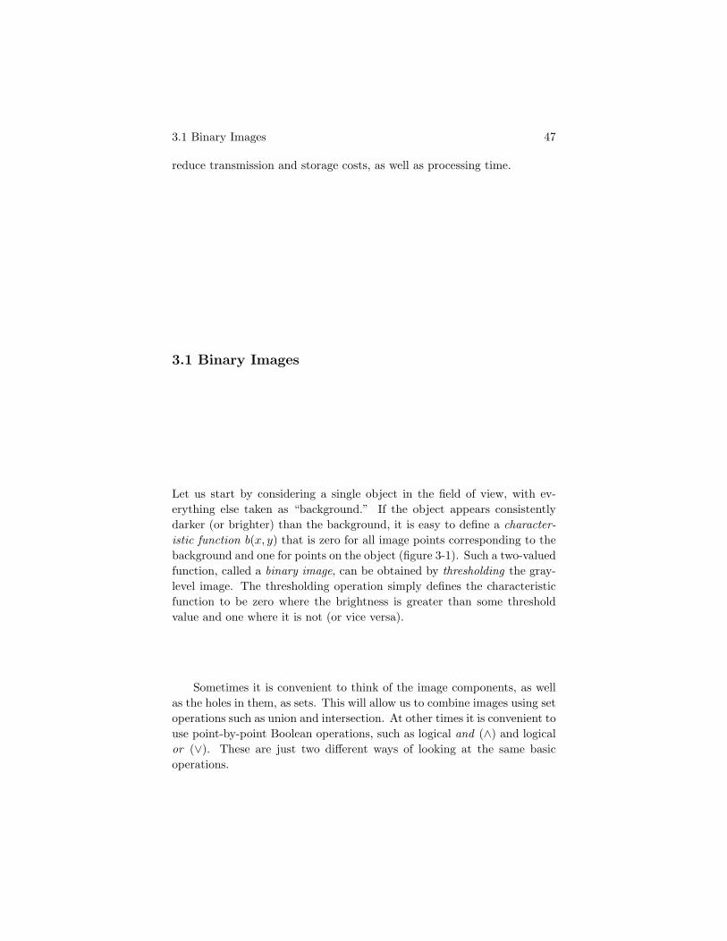
Let us start by considering a single object in the field of view, with ev-erything else taken as “background.” If the object appears consistentlydarker (or brighter) than the background, it is easy to define a character-istic function b(x, y) that is zero for all image points corresponding to thebackground and one for points on the object (figure 3-1). Such a two-valuedfunction, called a binary image, can be obtained by thresholding the gray-level image. The thresholding operation simply defines the characteristicfunction to be zero where the brightness is greater than some thresholdvalue and one where it is not (or vice versa).

Sometimes it is convenient to think of the image components, as wellas the holes in them, as sets. This will allow us to combine images using setoperations such as union and intersection. At other times it is convenient touse point-by-point Boolean operations, such as logical and (∧) and logicalor (∨). These are just two different ways of looking at the same basicoperations.

48 Binary Images: Geometric Properties

For a given image size, a binary image is easier to digitize, store, andtransmit than a full gray-level image, since it contains about an order ofmagnitude fewer bits. Naturally, some information is lost and fewer optionsare open to us in processing such an image. In fact, we can present afairly complete theory of what can and cannot be done with binary images,something that still eludes us in the case of gray-level images.

First of all, we can compute various geometric properties, such as thesize and position of the object in the image. If there is more than oneobject in the field of view, we can determine some topological propertiesof the assembly, such as the difference between the number of objects andthe number of holes. It is also possible to label the individual objects andto perform the geometrical computations for each one separately. Finally,we can simplify binary images for further processing by modifying them inan iterative fashion.

Binary image processing is well understood and lends itself to high-speed hardware implementation, but one must keep in mind its limitations.We have already mentioned the need for high object-to-background con-trast. Moreover, the pattern obtained must be essentially two-dimensional.Remember that all we have is the outline or silhouette of the object. Thisgives little information about the object’s overall shape or its attitude inspace.

The characteristic function b(x, y) has a value for each point in theimage. We call this a continuous binary image. Later, we shall considerdiscrete binary images, obtained by tessellating the image plane suitably.

3.2 Simple Geometrical Properties

Assume for now that we have a single object in the field of view. Thearea of the object, given the characteristic function b(x, y), can be foundas follows:

A =∫∫

I

b(x, y) dx dy,

where the integration is over the whole image I. If there is more than oneobject, this formula will give the total area.

3.2.1 Area and Position

How do we determine the position of the object in the image? Since theobject is usually not just a single point, we must give a precise meaningto the term “position.” The usual practice is to choose the center of areaas the representative point (figure 3-2). The center of area is the center of

3.2 Simple Geometrical Properties 49

mass of a figure of the same shape with constant mass per unit area. Thecenter of mass, in turn, is that point where all the mass of the object couldbe concentrated without changing the first moment of the object about anyaxis. In the two-dimensional case the moment about the x-axis is

x

∫∫I

b(x, y) dx dy =∫∫

I

x b(x, y) dx dy,

and the moment about the y-axis is

y

∫∫I

b(x, y) dx dy =∫∫

I

y b(x, y) dx dy,

where (x, y) is the position of the center of area. The integrals appearingon the left of these equations are, of course, just the area A, as noted above.To find x and y we must assume that A is not equal to zero. Note, by theway, that A is the zeroth moment of b(x, y).

3.2.2 Orientation

We also want to determine how the object lies in the field of view, thatis, its orientation. This is a little harder. Let us assume that the object


is somewhat elongated; then the orientation of the axis of elongation canbe used to define the orientation of the object (figure 3-3). (There is aremaining two-way ambiguity, however, as discussed in exercise 3-7.) Howprecisely do we define the direction in which the object is elongated? Theusual practice is to choose the axis of least second moment. This is thetwo-dimensional equivalent of the axis of least inertia. We find the line forwhich the integral of the square of the distance to points in the object is aminimum; that integral is

E =∫∫

I

r2b(x, y) dx dy,

where r is the perpendicular distance from the point (x, y) to the line sought


after.


To choose a particular line in the plane, we need to specify two pa-rameters. A convenient pair consists of the distance ρ from the origin tothe closest point on the line, and the angle θ between the x-axis and theline, measured counterclockwise (figure 3-4). We prefer these parametersbecause they change continuously when the coordinate system is trans-lated or rotated. There are no problems when the line is parallel, or nearlyparallel, to either of the coordinate axes.

Using these parameters, we can write the equation of the line in theform

x sin θ − y cos θ + ρ = 0

by noting that the line intersects the x-axis at −ρ/ sin θ and the y-axis at +ρ/ cos θ. The closest point on the line to the origin is at(−ρ sin θ, +ρ cos θ). We can write parametric equations for points on theline as follows:

x0 = −ρ sin θ + s cos θ and y0 = +ρ cos θ + s sin θ,


where s is the distance along the line from the point closest to the origin.


Given a point (x, y) on the object, we need to find the closest point(x0, y0) on the line, so that we can compute the distance r between thepoint and the line (figure 3-5). Clearly

r2 = (x − x0)2 + (y − y0)2.

Substituting the parametric equations for x0 and y0 we obtain

r2 = (x2 + y2) + ρ2 + 2ρ(x sin θ − y cos θ) − 2s(x cos θ + y sin θ) + s2.

Differentiating with respect to s and setting the result equal to zero leadto

s = x cos θ + y sin θ.

This result can now be substituted back into the parametric equations forx0 and y0. From these we can compute the differences

x − x0 = + sin θ (x sin θ − y cos θ + ρ) ,

y − y0 = − cos θ (x sin θ − y cos θ + ρ) ,

and thus

r2 = (x sin θ − y cos θ + ρ)2.

Comparing this result with the equation for the line, we see that the line isthe locus of points for which r = 0! Conversely, it becomes apparent thatthe way we chose to parameterize the line has the advantage of giving us


the distance from the line directly.


Finally, we can now address the minimization of

E =∫∫

I

(x sin θ − y cos θ + ρ)2 b(x, y) dx dy.

Differentiating with respect to ρ and setting the result to zero lead to

A(x sin θ − y cos θ + ρ) = 0,

where (x, y) is the center of area defined above. Thus the axis of leastsecond moment passes through the center of area. This suggests a changeof coordinates to x′ = x − x and y′ = y − y, for

x sin θ − y cos θ + ρ = x′ sin θ − y′ cos θ,

and soE = a sin2 θ − b sin θ cos θ + c cos2 θ,

where a, b, and c are the second moments given by

a =∫∫

I′(x′)2 b(x, y) dx′ dy′,

b = 2∫∫

I′(x′y′) b(x, y) dx′ dy′,

c =∫∫

I′(y′)2 b(x, y) dx′ dy′.

Now we can write the formula for E in the form

E =12(a + c) − 1

2(a − c) cos 2θ − 1

2b sin 2θ.

Differentiating with respect to θ and setting the result to zero, we have

tan 2θ =b

a − c,

unless b = 0 and a = c. Consequently

sin 2θ = ± b√b2 + (a − c)2

and cos 2θ = ± a − c√b2 + (a − c)2

.

Of the two solutions, the one with the plus signs in the expressions for sin 2θand cos 2θ leads to the desired minimum for E. Conversely, the solutionwith minus signs in the two expressions corresponds to the maximum valuefor E. (This can be shown by considering the second derivative of E withrespect to θ.) If b = 0 and a = c, we find that E is independent of θ. In

3.3 Projections 61

this case, the object is too symmetric to allow us to define an axis in thisway. The ratio of the smallest value for E to the largest tells us somethingabout how “rounded” the object is. This ratio is zero for a straight lineand one for a circle.

Another way to look at the problem is to seek the rotation θ that makesthe 2×2 matrix of second moments diagonal. We show in exercise 3-5 thatthe calculation above essentially amounts to finding the eigenvalues andeigenvectors of the 2 × 2 matrix of second moments given by

(a b/2

b/2 c

).

3.3 Projections

The position and orientation of an object can be calculated using first andsecond moments only. (There is a remaining two-way ambiguity, however,as discussed in exercise 3-7.) We do not need the original image to obtainthe first and second moments; projections of the image are sufficient. Thisis of interest since the projections are more compact and suggest much


faster algorithms.

3.3 Projections 63


Consider a line through the origin inclined at an angle θ with respect tothe x-axis (figure 3-6). Now construct a new line, intersecting the originalline at right angles, at a point that is a distance t from the origin. Letdistance along the new line be designated s. The integral of b(x, y) alongthe new line gives one value of the projection. That is,

pθ(t) =∫

L

b(t cos θ − s sin θ, t sin θ + s cos θ) ds.

The integration is carried out over the portion of the line L that lies withinthe image. The vertical projection (θ = 0), for example, is simply

v(x) =∫

L

b(x, y) dy,

while the horizontal projection (θ = π/2) is

h(y) =∫

L

b(x, y) dx.

Now, since

A =∫∫

I

b(x, y) dx dy,

we have

A =∫

v(x) dx =∫

h(y) dy.

More important,

xA =∫∫

I

x b(x, y) dx dy =∫

x v(x) dx

and

yA =∫∫

I

y b(x, y) dx dy =∫

y h(y) dy.

Thus the first moments of the projections are equal to the first momentsof the original image.

To compute orientation we need the second moments, too. Two ofthese are easy to compute from the projections:∫∫

I

x2 dx dy =∫

x2v(x) dx and∫∫

I

y2 dx dy =∫

y2h(y) dy.

We cannot, however, compute the integral of the product xy from thetwo projections introduced so far. We can add the diagonal projection

3.3 Projections 65

(θ = π/4),

d(t) =∫

b

(1√2(t − s),

1√2(t + s)

)ds.

Now consider that

∫∫I

12(x + y)2 b(x, y) dx dy =

∫∫I

t2 b(x, y) ds dt =∫

t2 d(t) dt,

and that

∫∫I

12(x + y)2 b(x, y) dx dy =

∫∫I

(12x2 + xy +

12y2

)b(x, y) dx dy.

So

∫∫I

xy b(x, y) dx dy =∫

t2d(t) dt − 12

∫x2v(x) dx − 1

2

∫y2h(y) dy.

Thus all the integrals needed for the computation of the position and ori-entation of a region in the binary image can be found from the horizontal,


diagonal, and vertical projections (figure 3-7).

3.3 Projections 67


It is interesting to compare tomographic reconstruction with what weare doing here. In tomography one obtains integrals of the absorbing den-sity of the material in some body. The problem is to reconstruct the dis-tribution of the material. In the case of X-ray tomography, the body iscommonly treated as a stack of slices, and each slice is considered a sep-arate two-dimensional problem. The projections obtained are analogousto the projections discussed above. It can be shown that the distributionof absorbing material can be determined if we have the projections for alldirections, provided that the density is zero outside some bounded region.

How does tomographic reconstruction relate to what we are doing here?The main difference is that in our case the function over which the line in-tegrals are taken can only have values zero and one. The other difference isthat we are not capturing sufficient information to reconstruct the originalbinary image, but only enough to determine the center of area and axis ofleast inertia. There are some interesting unsolved problems in the recon-struction of binary images from projections. Suppose, for example, thatthere is only one region that is nonzero and that this region is convex. Howmany projections are required to determine fully the outline of the region?Further, are there any noncircular shapes that have the same horizontal

3.3 Projections 69

and vertical projections as a circle?

3.5 Run-Length Coding 71

3.4 Discrete Binary Images

So far we have dealt with continuous binary images, defined at all pointsin the image plane. It should be obvious that the integrals become sumswhen we turn to discrete binary images (figure 3-8). The area, for example,can be computed (in units of the area of a picture cell) using the sum

A =n∑

i=1

m∑j=1

bij ,

where bij is the value of the binary image at the point in the ith row andthe jth column. Here we have assumed that the image has been digitizedon a square grid with n rows and m columns.

Usually the image is scanned out row by row, in the same sequence asthe beam on a television set explores the screen (except for interlace). Aseach picture cell is read, we check whether bij = 1. If so, we add 1, i, j,i2, ij, and j2 to the accumulated totals for the area, first moments, andsecond moments, as appropriate. At the end of the scan, the area, position,and orientation can be easily calculated from these totals.

3.5 Run-Length Coding

For binary images there are several coding techniques that can compressthe data even further. A popular one is run-length coding. This methodexploits the fact that along any particular scan line there will usually belong runs of zeros or ones. Instead of transmitting the individual bits, then,we can send numbers indicating the lengths of such runs. The run-lengthcode for the image line

0 1 1 1 1 0 0 0 1 1 0 0 0 0

is just [1, 4, 3, 2, 4]. Some special code may be used to indicate the beginningof each line. Further, a convention is followed as to whether the line startswith a zero or a one. If the line starts the other way, an initial run-lengthcode of zero is sent.

Let us use the convention that rik is the kth run of the ith line andthat the first run in each row is a run of zeros. (Thus all the even runswill correspond to ones in the image.) Suppose further that there are mi

runs on the ith line. (This number will be odd if the last run containszeros.) How do we use run-length codes to rapidly compute the desired


geometric properties? Clearly the area is just the sum of the run lengthscorresponding to ones in the image:

A =n∑

i=1

mi/2∑k=1

ri,2k.

Note that the sum is over the even runs only. The center of area is alittle harder to calculate. First of all, we obtain the horizontal projection(figure 3-9) as follows:

hi =mi/2∑k=1

ri,2k.

From this we can easily compute the vertical position i of the center of areausing

Ai =n∑

i=1

i hi.

But what about the vertical projection vj? Remember that a particularentry in this projection is obtained by adding up all picture cell valuesin one column of the image. It is therefore hard to compute the vertical


projection directly from the run lengths.

3.6 References 77

Now consider instead the first difference of the vertical projection,

vj = vj − vj−1, with v1 = v1.

Clearly it can be obtained by projecting not the image data, but the firsthorizontal differences of the image data:

bi,j = bi,j − bi,j−1.

The first difference bij has the advantage over bij itself that it is nonzeroonly at the beginning of each run. It equals +1 where the data change froma 0 to a 1, and −1 where the data change from a 1 to a 0 (figure 3-10). Wecan locate these places by computing the summed run-length code r̃ik:

r̃ik = 1 +k∑

l=1

ril

or, recursively, r̃i,0 = 1 and r̃i,j+1 = r̃i,j + ri,j . Then, for a transition atj = r̃ik we add (−1)k+1 to the accumulated total for the first difference ofthe vertical projection vj .

From this first difference we can compute the vertical projection itselfusing the simple summation

vj =j∑

l=1

vl,

or, recursively, v0 = 0 and vj+1 = vj + vj+1. The computation is illus-trated figure 3-10. Given the vertical projection, we can easily computethe horizontal position j of the center of area using

Aj =m∑

j=1

j vj .

We shall show in exercise 3-8 that the diagonal projection can be obtainedin a way similar to that used to obtain the vertical projection.

3.6 References

Another discussion of binary image processing can be found in Digital Pic-ture Processing by Rosenfeld & Kak [1982]. The book edited by Stoffel,Graphical and Binary Image Processing and Applications [1982], containssome interesting recent work in binary image processing. To see implemen-tations of some of the algorithms discussed here, look in the chapter on


binary image processing in Lisp, by Winston & Horn [1984]. Many inter-esting binary images produced by artists can be found in Silhouettes—APictorial Archive of Varied Illustrations, edited by Grafton [1979].

Run-length coding only exploits redundancy along one dimension.There have been several attempts to make use of spatial coherence in twodimensions in order to reduce transmission and storage costs. Perhaps themost successful scheme of this nature so far is that developed by IBM anddescribed by Mitchell & Goertzel [1979]. Further references relating tobinary image processing may be found at the end of the next chapter.

Simon Kahan of Bell Labs has solved one of the problems at the endof section 3.3. He has proven that no noncircular shape has the samehorizontal and vertical projections as a circle.

3.7 Exercises

3-1 The extreme values of the moment of inertia can be written as

E =12(a + c) ± 1

2

√b2 + (a − c)2,

where a, b, and c are as defined in this chapter. Show that E ≥ 0. When isE = 0?

3-2 Rewrite the expression for the second moment about an axis inclined byan angle θ,

E =12(a + c) − 1

2(a − c) cos 2θ − 1

2b sin 2θ,

in the formE =

12(a + c) +

√b2 − (a − c)2 cos 2(θ − φ).

What is the angle φ?

3-3 Let a, b, and c be the integrals defined in this chapter.

(a) Write a, b, and c in terms of integrals over x and y, instead of x′ and y′.(b) Find expressions for sin θ and cos θ from the expressions given for sin 2θ and

cos 2θ.

3-4 It is useful, at times, to replace a shape with one that is simpler but hasthe same zeroth, first, and second moments. Consider a region whose boundaryis an ellipse with semimajor axis α along the x-axis and semiminor axis β alongthe y-axis. The equation of this ellipse is(

x

α

)2+

(y

β

)2= 1.

3.7 Exercises 79

Show that the minimum and maximum second moments of the region about anaxis through the origin are

π

4αβ3 and

π

4βα3,

respectively. Now the second moment of any region about an axis inclined at anangle θ can be written in the form

E = a sin2 θ − b sin θ cos θ + c cos2 θ.

Compute the major and minor axes of an equivalent ellipse, that is, one that hasthe same second moment about any axis through the origin.

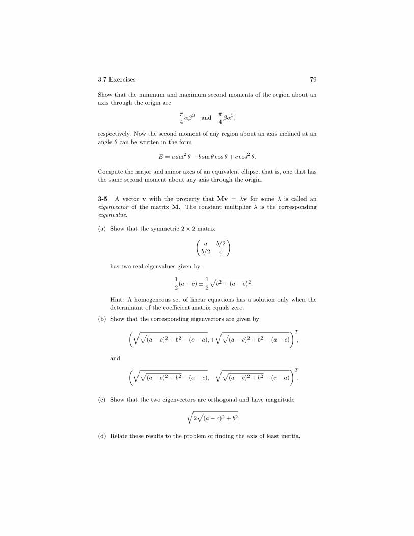
3-5 A vector v with the property that Mv = λv for some λ is called aneigenvector of the matrix M. The constant multiplier λ is the correspondingeigenvalue.

(a) Show that the symmetric 2 × 2 matrix(a b/2

b/2 c

)

has two real eigenvalues given by

12(a + c) ± 1

2

√b2 + (a − c)2.

Hint: A homogeneous set of linear equations has a solution only when thedeterminant of the coefficient matrix equals zero.

(b) Show that the corresponding eigenvectors are given by

(√√(a − c)2 + b2 − (c − a), +

√√(a − c)2 + b2 − (a − c)

)T

,

and (√√(a − c)2 + b2 − (a − c), −

√√(a − c)2 + b2 − (c − a)

)T

.

(c) Show that the two eigenvectors are orthogonal and have magnitude√2√

(a − c)2 + b2.

(d) Relate these results to the problem of finding the axis of least inertia.


3-6 Show how the integral ∫∫I

xy b(x, y) dx dy

can be computed from the horizontal and vertical projections and a projectionpθ(t) at angle θ, where

pθ(t) =∫

b(t cos θ − s sin θ, t sin θ + s cos θ) ds.

What restriction must be placed on θ ?

3-7 The axis of least inertia uniquely defines a line through an object. Themethods introduced so far do not, however, assign an orientation to this line.This two-way ambiguity in determining orientation may be significant in someapplications. One can use auxiliary measurements to provide the needed extrabit of information. For example, it may be helpful to know where the point onthe silhouette is that is furthest from the center of area.

Alternatively, we can consider computing higher-order moments. How manyprojections are required to find all moments up to the third? Which projectionsare most conveniently added to the ones we already have, that is, the horizontal(→), the vertical (↓), and the diagonal from NW to SE (↘)?

3-8 Show exactly how diagonal projections in the NW-to-SE (↘) and NE-to-SW (↙) directions can be computed from the run lengths.

3-9 If the scan line is very long, many bits must be reserved for each run-lengthnumber (for 4, 096 picture cells, 12-bit numbers are needed). This is wasteful ifmost runs are short. Devise a scheme in which shorter numbers are sent.

3-10 Can the run-length code ever be less compact than the original image? Ifso, suggest preprocessing methods that might alleviate the problem.

3-11 Assuming a fixed picture, estimate how the number of bits increases whenthe number of rows and the number of columns are doubled. Consider bothstraightforward binary encoding as well as run-length coding of the image.

3-12 Suppose we have the following runs, rik:

1 4 2 5 2

1 8 1 3 1

2 6 2 2 2

3.7 Exercises 81

Find the summed run-length codes rik. From these find vj , the first differenceof the vertical projection. Show that the vertical projection vj is

0 2 3 3 3 2 2 3 2 1 3 3 1 0

3-13 In this chapter we have assumed that a binary image is represented by amatrix of zeros and ones. We might equally well use a list of the boundary curvesof the regions in the image. Each boundary could be approximated by a polygon,for example. Show that the area of a region R can be computed as follows:

A = +∮

∂R

x dy = −∮

∂R

y dx,

where the integrals are taken in a counterclockwise fashion around the boundary∂R of the region R. Develop similar integrals for the first and second momentsneeded in the computation of the center of area and the axis of least inertia. Hint:Use Gauss’s integral theorem for converting area integrals into loop integrals.

3 Binary Images: Geometric Properties - MIT...

Documents

Transcript of 3 Binary Images: Geometric Properties - MIT...