Geometry and Computing 4

Geometric Algebra with Applications in Engineering

Bearbeitet vonChristian Perwass

1. Auflage 2008. Buch. xiv, 386 S. HardcoverISBN 978 3 540 89067 6

Format (B x L): 15,5 x 23,5 cmGewicht: 760 g

Weitere Fachgebiete > Mathematik > Geometrie > Algebraische Geometrie

Zu Inhaltsverzeichnis

schnell und portofrei erhältlich bei

Die Online-Fachbuchhandlung beck-shop.de ist spezialisiert auf Fachbücher, insbesondere Recht, Steuern und Wirtschaft.Im Sortiment finden Sie alle Medien (Bücher, Zeitschriften, CDs, eBooks, etc.) aller Verlage. Ergänzt wird das Programmdurch Services wie Neuerscheinungsdienst oder Zusammenstellungen von Büchern zu Sonderpreisen. Der Shop führt mehr

als 8 Millionen Produkte.

Chapter 1

Introduction

Geometric algebra is currently not a widespread mathematical tool in thefields of computer vision, robot vision, and robotics within the engineer-ing sciences, where standard vector analysis, matrix algebra, and, at times,quaternions are mainly used. The prevalent reason for this state of affairs isprobably the fact that geometric algebra is typically not taught at universi-ties, let alone at high-school level, even though it appears to be the mathe-matical language for geometry. This unfortunate situation seems to be due totwo main aspects. Firstly, geometric algebra combines many mathematicaltools that were developed separately over the past 200-odd years, such asthe standard vector analysis, Grassmann’s algebra, Hamilton’s quaternions,complex numbers, and Pauli matrices. To a certain extent, teaching geomet-ric algebra therefore means teaching all of these concepts at once. Secondly,most applications in two- and three-dimensional space, which are the mostcommon spaces in engineering applications, can be dealt with using standardvector analysis and matrix algebra, without the need for additional tools.The goal of this text is thus to demonstrate that geometric algebra, whichcombines geometric transformations with the construction and intersectionof geometric entities in a single framework, can be used advantageously inthe analysis and solution of engineering applications.

Matrix algebra, or linear algebra in general, probably represents the mostversatile mathematical tool in the engineering sciences. In fact, any geometricalgebra can be represented in matrix form, or, more to the point, geometricalgebra is a particular subalgebra of general tensor algebra (see e.g. [148]).However, this constraint can be an advantage, as for example in the case ofquaternions, which form a subalgebra of geometric algebra. While rotationsabout an axis through the origin in 3D space can be represented by 3 × 3matrices, it is a popular method to use quaternions instead, because theircomponents are easier to interpret (direction of rotation axis and rotationangle) and, with only four parameters, they are a nearly minimal parameter-ization. Given the four components of a quaternion, the corresponding (scal-ing) rotation is uniquely determined, whereas the three Euler angles from

C. Perwass, Geometric Algebra with Applications in Engineering.Geometry and Computing.c© Springer-Verlag Berlin Heidelberg 2009

1

2 1 Introduction

which a rotation matrix can be constructed do not suffice by themselves. Itis also important to define in which order the three rotations about the threebasis axes are executed, in order to obtain the correct rotation matrix. It isalso not particularly intuitive what type of rotation three Euler angles repre-sent. This is the reason why, in computer graphics software libraries such asOpenGL [23, 22], rotations are always given in terms of a rotation axis anda rotation angle. Internally, this is then transformed into the correspondingrotation matrices.

Apart from the obvious interpretative advantages of quaternions, there areclear numerical advantages, at the cost that only rotations can be described,whereas matrices can represent any linear function. For example, two rota-tions are combined by multiplying two quaternions or two rotation matrices.The product of two quaternions can be represented by the product of a 4× 4matrix with a 4× 1 vector, while in the case of a matrix representation two3×3 matrices have to be multiplied. That is, the former operation consists of16 multiplications and 12 additions, while the latter needs 27 multiplicationsand 18 additions. Furthermore, when one is solving for a rotation matrix, twoadditional constraints need to be imposed on the nine matrix components:matrix orthogonality and scale. In the case of quaternions, the orthogonalityconstraint is implicit in the algebraic structure and thus does not have to beimposed explicitly. The only remaining constraint is therefore the quaternionscale.

The quaternion example brings one of the main advantages of geomet-ric algebra to the fore: by reducing the representable transformations fromall (multi)linear functions to a particular subset, for example rotation, amore optimal parameterization can be achieved and certain constraints onthe transformations are embedded in the algebraic structure. In other words,the group structure of a certain set of matrices is made explicit in the algebra.On the downside, this implies that only a subset of linear transformations isdirectly available. Clearly, any type of function, including linear transforma-tions, can still be defined on algebraic entities, but not all functions profit inthe same way from the algebraic structure.

The above discussion gives an indication of the type of problems wheregeometric algebra tends to be particularly beneficial: situations where onlya particular subset of transformations and/or geometric entities are present.The embedding of appropriate constraints in the algebraic structure can thenlead to descriptive representations and optimized numerical constraints.

One area where the embedding of constraints in the algebraic structurecan be very valuable is the field of artificial neural networks, or classifica-tion algorithms in general. Any classification algorithm has to make someassumptions about the structure of the feature space or, rather, the form ofthe separation boundaries between areas in the feature space that belong todifferent classes. Choosing the best basis functions (kernels) for such a sepa-ration can improve the classification results considerably. geometric algebraoffers, through its algebraic structure, methods to advantageously implement

1.1 History 3

such basis functions, in particular for geometric constraints. This has beenshown, for example, by Buchholz and Sommer [27, 29, 28] and by Bayro-Corrochano and Buchholz [17]. Banarer, Perwass, and Sommer have shown,furthermore, that hyperspheres as represented in the geometric algebra ofconformal space are effective basis functions for classifiers [134, 14, 15]. Inthis text, however, these aspects will not be detailed further.

1.1 History

Before discussing further aspects of geometric algebra, it is helpful to lookat its roots. Geometric algebra is basically just another name for Cliffordalgebra, a name that was introduced by David Hestenes to emphasize thegeometric interpretation of the algebra. He first published his ideas in a re-fined version of his doctoral thesis in 1966 [87]. A number of books extendingthis initial “proof of concept” (as he called it) followed in the mid 1980s andearly 1990s [91, 88, 92]. Additional information on his current projects canbe found on the website [90].

Clifford algebra itself is about 100 years older. It was developed by WilliamK. Clifford (1845–1879) in 1878 [37, 35]. A collection of all his papers canbe found in [36]. Clifford’s main idea was that the Ausdehnungslehre of Her-mann G. Grassmann (1809–1877) and the quaternion algebra of William R.Hamilton (1805–1865) could be combined in a single geometric algebra, whichwas later to be known as Clifford algebra. Unfortunately, Clifford died veryyoung and had no opportunity to develop his algebra further. In around 1881the physicist Josiah W. Gibbs (1839–1903) developed a method that made iteasier to deal with vector analysis, which advanced work on Maxwell’s elec-trodynamics considerably. This was probably one of the reasons why Gibbs’svector analysis became the standard mathematical tool for physicists and en-gineers, instead of the more general but also more elaborate Clifford algebra.

Within the mathematics community, the Clifford algebra of a quadraticmodule was a well-established theory by the end of the 1970s. See, for ex-ample, the work of O’Meara [129] on the theory over fields or the work ofBaeza [13] on the theory over rings. The group structure of Clifford algebrawas detailed by, for example, Porteous [148] and Gilbert and Murray [79]in the 1990s. The latter also discussed the relation between Clifford algebraand Dirac operators, which is one of the main application areas of Cliffordalgebra in physics.

The Dirac equation of quantum mechanics has a natural representation inClifford algebra, since the Pauli matrices that appear in it form an algebrathat is isomorphic to a particular Clifford algebra. Some other applicationsof Clifford algebra in physics are to Maxwell’s equations of electrodynamics,which have a very concise representation, and to a flat-space theory of gravity

4 1 Introduction

[46, 106]. An introduction to geometric algebra for physicists was publishedby Doran and Lasenby in 2003 [45].

The applications of Clifford algebra or geometric algebra in engineeringwere initially based on the representation of geometric entities in projectivespace, as introduced by Hestenes and Ziegler in [92]. These were, for exam-ple, applications to projective invariants (see e.g. [107, 108]) and multiple-view geometry (see e.g. [18, 145, 144]). Initial work in the field of roboticsused the representation of rotation operators in geometric algebra (see e.g.[19, 161]). The first collections of papers discussing applications of geometricalgebra in engineering appeared in the mid 1990s [16, 48, 164, 165]. The firstdesign of a geometric algebra coprocessor and its implementation in a field-programmable gate array (FPGA) was developed by Perwass, Gebken, andSommer in 2003 [137].

In 2001 Hongbo Li, David Hestenes, and Alyn Rockwood published threearticles in [164] introducing the conformal model [116], spherical conformalgeometry [117], and a universal model for conformal geometries [118]. Thesearticles laid the foundation for a whole new class of applications that could betreated with geometric algebra. Incidentally, Pierre Angles had already devel-oped this representation of the conformal model independently in the 1980s[6, 7, 8] but, apparently, it was not registered by the engineering community.His work on conformal space can also be found in [9].

The conformal model is based on work by Friedrich L. Wachter (1792–1817), a student of J. Carl F. Gauss (1777–1855), who showed that a certainsurface in hyperbolic geometry was metrically equivalent to Euclidean space.Forming a geometric algebra over a homogeneous embedding of this spaceextends the representation of points, lines, planes, and rotations about axesthrough the origin to point pairs, circles, spheres, and conformal transforma-tions, which include all Euclidean transformations. Note that the representa-tion of Euclidean transformations in the conformal model is closely related tobiquaternions, which had been investigated by Clifford himself in 1873 [34],a couple of years before he developed his algebra. The extended set of ba-sic geometric entities in the conformal model and the additionally availabletransformations made geometric algebra applicable to a larger set of appli-cation areas, for example pose estimation [155, 152], a new type of artificialneural network [15], and the description of space groups [89].

Although the foundations of the conformal model were laid by Li, Hestenes,and Rockwood in 2001, its various facets, properties, and extensions are stilla matter of ongoing research (see e.g. [49, 105, 140, 160]). One of the aimsof this text is to present the conformal model in the context of other geo-metric algebra models and to give a detailed derivation of the model itself,as well as in-depth discussions of its geometric entities and transformationoperators. Even though the conformal model is particularly powerful, it ispresented as one special case of a general method for representing geometryand transformations with geometric algebra. One result of this more generaloutlook is the geometric algebra of conic space, which is published here in

1.2 Geometry 5

all of its details for the first time. In this geometric algebra, the algebraicentities represent all types of projective conic sections.

1.2 Geometry

One of the novel features of the discussion of geometric algebra in this textis the explicit separation of the algebra from the representation of geometrythrough algebraic entities. In the author’s opinion this is an advantageousview, since it clarifies the relation between the various geometric modelsand indicates how geometric algebra may be developed for new geometricmodels. The basic idea that blades represent linear subspaces through theirnull space has already been noted by Hestenes. However, the consequentexplicit application of this notion to the discussion of different geometricmodels and algebraic operations was first developed in [140] and is extendedin this text. Note that the notion of representing geometry through null spacesis directly related to affine varieties in algebraic geometry [38].

One conclusion that can be drawn from this view of geometric algebra isthat there exist only three fundamental operations in the algebra, all based onthe same algebraic product: “addition”, “subtraction”, and reflection of linearsubspaces. All geometric entities, such as points, lines, planes, spheres, circles,and conics, are represented through linear subspaces, and all transformations,such as rotation, inversion, translation, and dilation, are combinations of re-flections of linear subspaces. Nonlinear geometric entities such as spheres andnonlinear transformations such as inversions stem from a particular embed-ding of Euclidean space in a higher-dimensional embedding space, such thatlinear subspaces in the embedding space represent nonlinear subspaces inthe Euclidean space, and combinations of reflections in the embedding spacerepresent nonlinear transformations in the Euclidean space. This aspect isdetailed further in Chap. 4, where a number of geometries are discussed indetail.

The fact that all geometric entities and all transformation operations areconstructed through fundamental algebraic operations leads to two key prop-erties of geometric algebra:

1. Geometric entities and transformation operators are constructed in ex-actly the same way, independent of the dimension of the space they areconstructed in.

2. The intersection operation and the transformation operators are the samefor all geometric entities in all dimensions.

For example, it is shown in Sect. 4.2 that in the geometric algebra of theprojective space of Euclidean 3D space R3, a vector A represents a point.The outer product (see Sect. 3.2.2) of two vectors A and B in this space,denoted by A ∧B, then represents the line through A and B. If A and B

6 1 Introduction

are vectors in the projective space of R10, say, they still represent points andA ∧B still represents the line through these points.

The intersection operation in geometric algebra is called the meet and isdenoted by ∨. If A and B represent any two geometric entities in any dimen-sion, then their intersection is always determined with the meet operation asA ∨B. Note that even if the geometric entities represented by A and B haveno intersection, the meet operation results in an algebraic entity. Typicallythis entity then represents an imaginary geometric object or one that lies atinfinity. This property of the intersection operation has the major advantagethat no additional checks have to be performed before the intersection of twoentities is computed.

The application of transformations is similarly dimension-independent. Forexample, if R is an algebraic entity that represents a rotation and A repre-sents any geometric entity, then RAR−1 represents the rotated geometricentity, independent of its type and dimension. Note that juxtaposition of twoentities denotes the algebra product, the geometric product.

To a certain extent, it can therefore be said that geometric algebra allowsa coordinate-free representation of geometry. Hestenes emphasized this prop-erty by developing the algebra with as little reference to a basis as possible in[87, 91]. However, since in those texts the geometric algebra over real-valuedvector spaces is discussed, a basis can always be found, but it is not essentialfor deriving the properties of the algebra. The concept of a basis-independentgeometric algebra was extended even further by Frank Sommen in 1997. Heconstructed a Clifford algebra completely without the notion of a vector space[162, 163]. In this approach abstract basic entities, called vector-variables, areconsidered, which are not entities of a particular vector space. Instead, thesevector-variables are characterized purely through their algebraic properties.An example of an application of this radial algebra is the construction ofClifford algebra on super-space [21].

The applications considered in this text, however, are all related to par-ticular vector spaces, which allows a much simpler construction of geometricalgebra. The manipulation of analytic expressions in geometric algebra is stillmostly independent of the dimensionality of the underlying vector space orany particular coordinates.

1.3 Outlook

From a mathematical point of view, geometric algebra is an elegant andanalytically powerful formalism to describe geometry and geometric trans-formations. However, the particular aim of the engineering sciences is thedevelopment of solutions to problems in practical applications. The toolsthat are used to achieve that aim are only of interest insofar as the executionspeed and the accuracy of solutions are concerned. Nevertheless, this does

1.3 Outlook 7

not preclude research into promising mathematical tools, which could lead toa substantial gain in application speed and accuracy or even new applicationareas. At the end of the day, though, a mathematical tool will be judged byits applicability to practical problems. In this context, the question has to beasked:

What are the advantages of geometric algebra?

Or, more to the point, when should geometric algebra be used? There appearsto be no simple, generally applicable answer to this question. Earlier in thisintroduction, some pointers were given in this context. Basically, geometricalgebra has three main properties:

1. Linear subspaces can be represented in arbitrary dimensions.2. Subspaces can be added, subtracted, and intersected.3. Reflections of subspaces in each other can be performed.

Probably the most important effects that these fundamental properties haveare the following:

• With the help of a non-linear embedding of Euclidean space, it is possi-ble to represent non-linear subspaces and transformations. This allows a(multi)linear representation of circles and spheres, and non-linear trans-formations such as inversions.

• The combination of the basic reflection operations results in more complextransformations, such as rotation, translation, and dilation. The corre-sponding transformation operators are nearly minimal parameterizationsof the transformation. Additional constraints, such as the orthogonality ofa rotation matrix, are encoded in the algebraic structure.

• Owing to the dimension-independent representation of geometric entities,only a single intersection operation is needed to determine the intersec-tions between arbitrary combinations of entities. This can be a powerfulanalytical tool for geometrical constructions.

• The dimension-independent representation of geometric entities and re-flections also has the effect that a transformation operator can be appliedto any element in the algebra in any dimension, be it a geometric entityor another transformation.

• Since all transformations are represented as multilinear operations, theuncertainty of Gaussian distributed transformation operators can be ef-fectively represented by covariance matrices. That is, the uncertainty ofgeometric entities and transformations can be represented in a unified fash-ion.

These properties are used in Chap. 6 to construct and estimate uncer-tain geometric entities and transformations. In Chap. 7, the availability ofa linearized inversion operator leads to a unifying camera model. Chapter 8exploits the encoding of transformation constraints in the algebraic structure.In Chap. 9, the dimension independence of the reflection operation leads to

8 1 Introduction

an immediate extension of Pythagorean-hodograph curves to arbitrary di-mensions. And Chap. 10 demonstrates the usefulness of representing linearsubspaces in the Hilbert space of random variables.

It is hoped that the subjects discussed in this text will help researchers toidentify advantageous applications of geometric algebra in their field.

1.4 Overview of This Text

This section gives an overview of the main contributions of this text in thecontext of research in geometric algebra and computer vision. The main aimof this text is to give a detailed presentation of and, especially, to developnew tools for the three aspects that are necessary to apply geometric algebrato engineering problems:

1. Algebra, the mathematical formalism.2. Geometry, the representation of geometry and transformations.3. Numerics, the implementation of numerical solution methods.

This text gives a thorough description of geometric algebra, presents thegeometry of the geometric algebra of Euclidean, projective, conformal, and anovel conic space in great detail, and introduces a novel numerical calculationmethod for geometric algebra that incorporates the notion of random algebravariables. The methodology presented combines the representative power ofthe algebra and its effective algebraic manipulations with the demands ofreal-life applications, where uncertain data is unavoidable.

A number of applications where this methodology is used are presented,which include the description of uncertain geometric entities and transforma-tions, a novel camera model, and monocular pose estimation with uncertaindata. In addition, applications of geometric algebra to some special polyno-mial curves (Pythagorean-hodograph curves), and the geometric algebra overthe Hilbert space of random variables are presented.

In addition to the mathematical contributions, the software tool CLU-Calc, developed by the author, is introduced. CLUCalc is a stand-alonesoftware program that implements geometric algebra calculations and, moreimportantly, can visualize the geometric content of algebraic entities auto-matically. It is therefore an ideal tool to help in the learning and teaching ofgeometric algebra.

In the remainder of this section, the main aspects of all chapters are de-tailed.

1.4 Overview of This Text 9

1.4.1 CLUCalc

The software tool CLUCalc (Chap. 2) [133] was developed by the authorwith the aim of furthering the understanding, supporting the teaching, andimplementing applications of geometric algebra. For this purpose, a wholenew programming language, called CLUScript, was developed, which washoned for the programming of geometric algebra expressions. For example,most operator symbols typically used in geometric algebra are available inCLUScript. However, probably the most useful feature in the context ofgeometric algebra is the automatic visualization of the geometric content ofmultivectors. That is, the user need not know what a multivector representsin order to draw it. Instead, the meaning of multivectors and the effect ofalgebraic operations can be discovered interactively. Since geometric algebrais all about geometry, CLUScript offers simple access to powerful visualiza-tion features, such as transparent objects, lighting effects, texture mapping,animation, and user interaction. It also supports the annotation of drawingsusing LATEX text, which can also be mapped onto arbitrary surfaces. Notethat virtually all of the figures in this text were created with CLUCalc, andthe various applications presented were implemented in CLUScript.

1.4.2 Algebra

One aspect that has been mentioned before is the clear separation of algebraicentities and their geometric interpretation. The foundation for this view islaid in Chap. 3 by introducing the inner- and outer-product null spaces. Thisconcept is extended to the geometric inner- and outer-product null spaces inChap. 4 on geometries, to give a general methodology of how to representgeometry by geometric algebra. Note that this concept is very similar to affinevarieties in algebraic geometry [38].

Another important aspect that is treated explicitly in Chap. 3 is thatof null vectors and null blades, which is something that is often neglected.Through the definition of an algebra conjugation, a Euclidean scalar productis introduced, which, together with a corresponding definition of the magni-tude of an algebraic entity, or multivector, allows the definition of a Hilbertspace over a geometric algebra. While this aspect is not used directly, alge-bra conjugation is essential in the general definition of subspace addition andsubtraction, which eventually leads to factorization algorithms for blades andversors that are also valid for null blades and null versors. Furthermore, apseudoinverse of null blades is introduced. The relevance of these operationsis very high when working with the conformal model, since geometric entitiesare represented by blades of null vectors. In order to determine the meet, i.e.the general intersection operation, between arbitrary blades of null vectors,a factorization algorithm for such blades has to be available.

10 1 Introduction

Independent of the null-blade aspect, a novel set of algorithms that areessential when implementing geometric algebra on a computer are presented.This includes, in particular, the evaluation of the join of blades, which isnecessary for the calculation of the meet. In addition, the versor factorizationalgorithm is noteworthy. This factorizes a general transformation into a setof reflections or, in the case of the conformal model, inversions.

1.4.3 Geometries

While the representation of geometric objects and transformations throughalgebraic entities is straightforward, extracting the geometric informationfrom the algebraic entities is not trivial. For example, in the conformal model,two vectors S1 and S2 can represent two spheres and their outer productC = S1 ∧ S2 the intersection circle of the two spheres (see Sect. 4.3.4).Extracting the circle parameters center, normal, and radius from the algebraicentity C is not straightforward. Nevertheless, a knowledge of how this canbe done is essential if the algebra is to be used in applications.

Therefore, the analysis of the geometric interpretation of algebraic entitiesthat represent elements of 3D Euclidean space is discussed in some detail.A somewhat more abstract discussion of the geometric content of algebraicentities in the conformal model of arbitrary dimension can be found in [116].Confining the discussion in this text to the conformal model of 3D Euclideanspace simplifies the formulas considerably.

Another important aspect of Chap. 4 is a discussion of how incidencerelations between geometric entities are represented through algebraic opera-tions. This knowledge is pivotal when one is expressing geometric constraintsin geometric algebra.

A particularly interesting contribution is the introduction of the conicspace, which refers to the geometric algebra over the vector space of re-duced symmetric matrices. In the geometric algebra of conic space, the outerproduct of five vectors represents the conic section that passes through thecorresponding five points. The outer product of four points represents a pointquadruplet, which is also the result of the meet of two five-blades, i.e. theintersection of two conic sections. The discussion of conic space starts outwith an even more general outlook, whereby the conic and conformal spacesare particular subspaces of the general polynomial space.

1.4.4 Numerics

The essential difference in the treatment of numerical calculation with ge-ometric algebra between this text and the standard approach introduced

1.4 Overview of This Text 11

by Hestenes is that algebraic operations in geometric algebra are regardedhere as bilinear functions and expressed through tensor contraction. This ap-proach was first introduced by the author and Sommer in [146]. While thestandard approach has its merits in the analytical description of derivativesas algebraic entities, the tensorial approach allows the direct application of(multi)linear optimization algorithms. At times, the tensorial approach alsoleads to solution methods that cannot be easily expressed in algebraic terms.

An example of the latter case is the versor equation (see Sect. 5.2.2).Without delving into all the details, the problem comes down to solving forthe multivector V , given multivectors A and B, the equation

V A−BV = 0 .

The problem is that it is impossible to solve for V through algebraic manip-ulations, since the various multivectors typically do not commute. However,in the tensorial representation of this equation, it is straightforward to solvefor the components of V by evaluating the null space of a matrix.

In the standard approach a function C(V ), say, would be defined as

C : V 7→ V A−BV .

The solution to V is then the vector V , that minimizes ∆(V ) := C(V ) ·C(V ). To evaluate V , the derivative of ∆(V ) with respect to V has to becalculated, which can be done with the multivector derivative introduced byHestenes [87, 91] (see Sect. 3.6). Then a standard gradient descent methodor something more effective can be used to find V . For an example of thisapproach, see [112]. It is shown in Sect. 5.2.2, however, that the tensorialapproach also minimizes ∆(V ); this method is much easier to apply.

Another advantage of the tensorial approach is that Gaussian distributedrandom multivector variables can be treated directly. This use of the tenso-rial approach was developed by the author in collaboration with W. Forstnerand presented at a Dagstuhl workshop in 2004 [136]. The present text ex-tends this and additional publications [76, 138, 139] to give a complete andthorough discussion of the subject area. The two main aspects with respectto random multivector variables, whose foundations are laid in Chap. 5, arethe construction and estimation of uncertain geometric entities and uncertaintransformations from uncertain data. For example, an uncertain circle canbe constructed from the outer product of three uncertain points, and an un-certain rotation operator may be constructed through the geometric productof two uncertain reflection planes.

The representation of uncertain transformation operators is certainly amajor advantage of geometric algebra over a matrix representation. This isdemonstrated in Sect. 5.6.1, where it is shown that the variation of a ran-dom transformation multivector in the conformal model, such as a rotationoperator, lies (almost) in a linear subspace. A covariance matrix is therefore

12 1 Introduction

well suited to representing the uncertainty of a Gaussian distributed randomtransformation multivector variable. It appears that the representation ofuncertain transformations with matrices is more problematic. Heuel investi-gated an approach whereby transformation matrices are written as columnvectors and their uncertainty as an associated covariance matrix [93]. Henotes that this method is numerically not very stable.

A particularly convincing example is the representation of rotations aboutthe origin in 3D Euclidean space. Corresponding transformation operators inthe conformal model lie in a linear subspace, which also forms a subalgebra,and a subgroup of the Clifford group. Rotation matrices, which are elementsof the orthogonal group, do not form a subalgebra at the same time. Thatis, the sum of two rotation matrices does not, in general, result in a rotationmatrix. A covariance matrix on a rotation matrix can therefore only representa tangential uncertainty.

Instead of constructing geometric entities and transformation operatorsfrom uncertain data, they can also be estimated from a set of uncertaindata. For this purpose, a linear least-squares estimation method, the Gauss–Helmert model, is presented (see Sect. 5.9), which accounts for uncertaintiesin measured data. Although this is a well-known method, a detailed derivationis given here, to hone the application of this method to typical geometric-algebra problems.

In computer vision, the measured data consists typically of the locationsof image points. Owing to the digitalization in CCD chips and/or the pointspread function (PSF) of the imaging system, there exists an unavoidableuncertainty in the position measurement. Although this uncertainty is usu-ally small, such small variations can lead to large deviations in a complexgeometric construction. Knowing the final uncertainty of the elements thatconstitute the data used in an estimation may be essential to determiningthe reliability of the outcome.

One such example is provided by a catadioptric camera, i.e. a camera witha 360 degree view that uses a standard projective camera which looks at aparabolic mirror. While it can be assumed that the uncertainties in the posi-tion of all pixels in the camera are equal, the uncertainty in the correspondingprojection rays reflected at the parabolic mirror varies considerably depend-ing on where they hit the mirror. Owing to the linearization of the inversionoperation in the conformal model, which can be used to model reflection ina parabolic mirror (see Sect. 7.2), simple error propagation can be used hereto evaluate the final uncertainty of the projection rays. These uncertain raysmay then form the data that is used to solve a pose estimation problem (seeChap. 8).

1.4 Overview of This Text 13

1.4.5 Uncertain Geometric Entities and Operators

In Chap. 6, the tools developed in Chap. 5 are applied to give examples ofthe construction and estimation of uncertain geometric entities and trans-formation operators. Here the construction of uncertain lines, circles, andconic sections from uncertain points is visualized, to show that the standard-deviation envelopes of such geometric entities are not simple surfaces. The useof a covariance matrix should always be favored over simple approximationssuch as a tube representing the uncertainty of a line.

Furthermore, the effect of an uncertain reflection and rotation on an idealgeometric entity is shown. This has direct practical relevance, for example,in the evaluation of the uncertainty induced in a light ray which is reflectedoff an uncertain plane.

With respect to the estimation of geometric entities and transformationoperators, standard problems that occur in the application of geometric al-gebra to computer vision problems are presented, and it is shown how themethods introduced in Chap. 5 can be used to solve them. In addition, themetrics used implicitly in these problems are investigated. This includes thefirst derivation of the point-to-circle metric and the versor equation metric.

The quality of the estimation methods presented is demonstrated in twoexperiments: the estimation of a circle and of a rotation operator. Both ex-periments demonstrate that the Gauss–Helmert method gives better resultsthan a simple null-space estimation. The estimation of the rotation opera-tor is also compared with a standard method, where it turns out that theGauss–Helmert method gives better and more stable results.

Another interesting aspect is hypothesis testing, where questions such as“does a point lie on a line?” are answered in a statistical setting. Here, thefirst visualization of what this means for the question “does a point lie on acircle?” in the conformal model is given (see Fig. 6.10).

1.4.6 The Inversion Camera Model

The inversion camera model is a novel camera model that was first publishedby Perwass and Sommer in [147]. In Chap. 7 an extended discussion of thiscamera model is given, which is applied in Chap. 8 to monocular pose es-timation. The inversion camera model combines the pinhole camera model,a lens distortion model, and the catadioptric-camera model for the case ofa parabolic mirror. All these configurations can be obtained by varying theposition of a focal point and an inversion sphere. Since inversion can be rep-resented through a linear operator in the conformal model, the geometricalgebra of conformal space offers an ideal framework for this camera model.The unification of three camera models that are usually treated separatelycan lead to generalized constraint equations, as is the case for monocular

14 1 Introduction

pose estimation. Note that the camera model is represented by a transfor-mation operator in the geometric algebra of conformal space, which impliesthat it can be easily associated with a covariance matrix that represents itsuncertainty.

1.4.7 Monocular Pose Estimation

In Chap. 8 an application is presented that uses all aspects of the previ-ously presented methodology: a geometric setup is translated into geometric-algebra expressions, algebraic operations are used to express a geometricconstraint, and a solution is found using the tensorial approach, which in-corporates uncertain data. While the pose estimation problem itself is wellknown, a number of novel aspects are introduced in this chapter:

• a simple and robust method to find an initial pose,• the incorporation of the inversion camera model into the pose constraint,• a pose constraint equation that is quadratic in the components of the pose

operator without making any approximations, and• the covariance matrix for the pose operator and the inversion camera model

operator.

The pose estimation method presented is thoroughly tested against groundtruth pose data generated with a robotic arm for a number of different imag-ing systems.

1.4.8 Versor Functions

In Chap. 9 some instances of versor functions are discussed, that is, functionsof the type F : t 7→ A(t)N A(t). One geometric interpretation of thistype of function is that a preimage A(t) scales and rotates a vector N . It isshown that cycloidal curves generated by coupled motors, Fourier series ofcomplex-valued functions, and Pythagorean-hodograph (PH) curves are allrelated to this form.

In the context of PH curves, a new representation based on the reflectionof vectors is introduced, and it is shown that this is equivalent to the standardquaternion representation in the case of cubic and quintic PH curves. Thisnovel representation has the advantage that it can be immediately extendedto arbitrary dimensions, and it gives a geometrically more intuitive repre-sentation of the degrees of freedom. This also leads to the identification ofparameter subsets that generate PH curves of constant length but of differentshape. The work on PH curves resulted from a collaboration of the authorwith R. Farouki [135].

1.5 Overview of Geometric Algebra 15

1.4.9 Random Variable Space

Chap. 10 gives an example of a geometric algebra over a general Hilbert space,instead of a real-valued vector space. The Hilbert space chosen here is that ofrandom variables. This demonstrates how the geometric concepts of geomet-ric algebra can be applied to function spaces. Some fundamental propertiesof random variables are presented in this context. This leads to a straight-forward derivation of the Cauchy–Schwarz inequality and an extension of thecorrelation coefficient to an arbitrary number of random variables. The ge-ometric insight into geometric algebra operations gained for the Euclideanspace can be applied directly to random variables, which gives properties suchas the expectation value, the variance, and the correlation a direct geometricmeaning.

1.5 Overview of Geometric Algebra

In this section, a mathematical overview of some of the most important as-pects of geometric algebra is presented. The purpose is to give those readerswho are not already familiar with geometric algebra a gentle introductionto the main concepts before delving into the detailed mathematical analysis.To keep it simple, only the geometric algebra of Euclidean 3D space is usedin this introduction and formal mathematical proofs are avoided. A detailedintroduction to geometric algebra is given in Chap. 3.

One problem in introducing geometric algebra is that depending on thereader’s background, different introductions are best suited. For pure mathe-maticians the texts on Clifford algebra by Porteous [148], Gilbert and Murray[79], Lounesto [119], Riesz [149], and Ablamowicz et al. [3], to name just afew, are probably most instructive. In this context, the text by Lounesto pre-senting counterexamples of theorems in Clifford algebra should be of interest[120].

The field of Clifford analysis is only touched upon when basic multivectordifferentiation is introduced in Sect. 3.6. This is sufficient to deal with thesimple functions of multivectors that are encountered in this text. Thoroughtreatments of Clifford analysis can be found in [24, 41, 42].

This text is geared towards the use of geometric algebra in engineeringapplications and thus stresses more those aspects that are related to the rep-resentation of geometry and Euclidean transformations. It may thus not treatall aspects that the reader is interested in. As always, the best way is to reada number of different introductions to geometric algebra. After the booksby Hestenes [87, 88, 91], there are a number of papers and books geared to-wards various areas, in particular physics and engineering. For physics-relatedintroductions see, for example [45, 83, 110], and for engineering-related in-troductions [47, 48, 111, 140, 50, 172].

16 1 Introduction

1.5.1 Basics of the Algebra

The real-valued 3D Euclidean vector space is denoted by R3, with an or-thonormal basis e1, e2, e3 ∈ R3. That is,

ei ∗ ej = δij , δij :=

{1 : i = j ,

0 : i 6= j ,

where ∗ denotes the standard scalar product. The geometric algebra of R3 isdenoted by G(R3), or simply G3. Its algebra product is called the geometricproduct, and is denoted by the juxtaposition of two elements. This is just asin matrix algebra, where the matrix product of two matrices is representedby juxtaposition of two matrix symbols. The effect of the geometric producton the basis vectors of R3 is

ei ej =

{ei ∗ ej : i = j ,

eij : i 6= j .(1.1)

One of the most important points to note for readers who are new to geo-metric algebra is the case when i 6= j, where eij ≡ ei ej represents a newalgebraic element, sometimes also denoted by eij for brevity. Similarly, ifi, j, k ∈ {1, 2, 3} are three different indices, eijk := ei ej ek is yet anothernew algebraic entity. That this process of creating new entities cannot becontinued indefinitely is ensured by defining the geometric product to beassociative and to satisfy ei ei = 1. The latter is also called the definingequation of the algebra. For example,

(ei ej ek) ek = (ei ej) (ek ek) = (ei ej) 1 = ei ej .

In Chap. 3 it is shown that (1.1) together with the standard axioms of anassociative algebra suffices to show that

ei ej = −ej ei if i 6= j . (1.2)

This implies, for example, that

(ei ej ek) ej = (ei ej) (ek ej) = −(ei ej) (ej ek) = −ei (ej ej) ek = −ei ek .

From these basic rules, the basis of G3 can be found to be

G3 :={

1, e1, e2, e3, e12, e13, e23, e123

}. (1.3)

In general, the dimension of the geometric algebra of an n-dimensional vectorspace is 2n.

1.5 Overview of Geometric Algebra 17

1.5.2 General Vectors

The operations introduced in the previous subsection are valid only for aset of orthonormal basis vectors. For general vectors of R3, the algebraicoperations have somewhat more complex properties, which can be related tothe properties of the basis vectors by noting that any vector a ∈ R3 can bewritten as

a := a1 e1 + a2 e2 + a3 e3 .

Note that the scalar components of the vector a, a1, a2, a3, are indexed bya superscript index. This notation will be particularly helpful when algebraoperations are expressed as tensor contractions. In particular, the Einsteinsummation convention can be used, which states that a subscript index re-peated as a superscript index within a product implies a summation over therange of the index. That is,

a := ai ei ≡3∑i=1

ai ei .

It is instructive to consider the geometric product of two vectors a, b ∈ R3

with a := ai ei and b := bi ei. Using the multiplication rules of the geometricproduct between orthonormal basis vectors as introduced in the previoussubsection, it is straightforward to find

ab = (a1 b1 + a2 b2 + a3 b3)

+ (a2 b3 − a3 b2) e23

+ (a3 b1 − a1 b3) e31

+ (a1 b2 − a2 b1) e12 .

(1.4)

Recall that e23, e31 and e12 are new basis elements of the geometric algebraG3. Because these basis elements contain two basis vectors from the vectorspace basis of R3, they are said to be of grade 2. Hence, the expression

(a2 b3 − a3 b2) e23 + (a3 b1 − a1 b3) e31 + (a1 b2 − a2 b1) e12

is said to be a vector of grade 2, because it is a linear combination of thebasis elements of grade 2.

The sum of scalar products in (1.4) is clearly the standard scalar productof the vectors a and b, i.e. a ∗ b. The grade 2 part can also be evaluatedseparately using the outer product. The outer product is denoted by ∧ anddefined as

ei ∧ ej =

{0 : i = j

ei ej : i 6= j(1.5)

18 1 Introduction

Since ei ∧ ej = ei ej if i 6= j, it is clear that ei ∧ ej = −ej ∧ ei. Also, notethat the expression ei ∧ ei = 0 is the defining equation for the Grassmann,or exterior, algebra (see Sect. 3.8.4). Therefore, by using the outer product,the Grassmann algebra is recovered in geometric algebra.

Using this definition of the outer product, it is not too difficult to showthat

a ∧ b = (a2 b3 − a3 b2) e23 + (a3 b1 − a1 b3) e31 + (a1 b2 − a2 b1) e12 ,

which is directly related to the standard vector cross product of R3, since

a× b = (a2 b3 − a3 b2) e1 + (a3 b1 − a1 b3) e2 + (a1 b2 − a2 b1) e3 .

To show how one expression can be transformed into the other, the conceptof the dual has to be introduced. To give an example, the dual of e1 is e2 e3,that is, the geometric product of the remaining two basis vectors. This canbe interpreted in geometric terms by saying that the dual of the subspaceparallel to e1 is the subspace perpendicular to e1, which is spanned by e2

and e3.A particularly powerful feature of geometric algebra is that this dual op-

eration can be expressed through the geometric product. For this purpose,the pseudoscalar I of G3 is defined as the basis element of highest grade,i.e. I := e1 e2 e3. Using again the rules of the geometric product, it fol-lows that the inverse pseudoscalar is given by I−1 = e3 e2 e1, such thatI I−1 = I−1 I = 1. The dual of some multivector A ∈ G3 is denoted by A∗

and can be evaluated viaA∗ = AI−1 .

It now follows that

(a ∧ b)∗ = (a ∧ b) I−1 = a× b .

What does this show? First of all, it shows that the important vector crossproduct can be recovered in geometric algebra. Even more importantly, itimplies that the vector cross product is only a special case, for a three-dimensional vector space, of a much more general operation: the outer prod-uct. Whereas the expression a ∧ b is a valid operation in any dimensiongreater than or equal to two, the vector cross product is defined only in threedimensions.

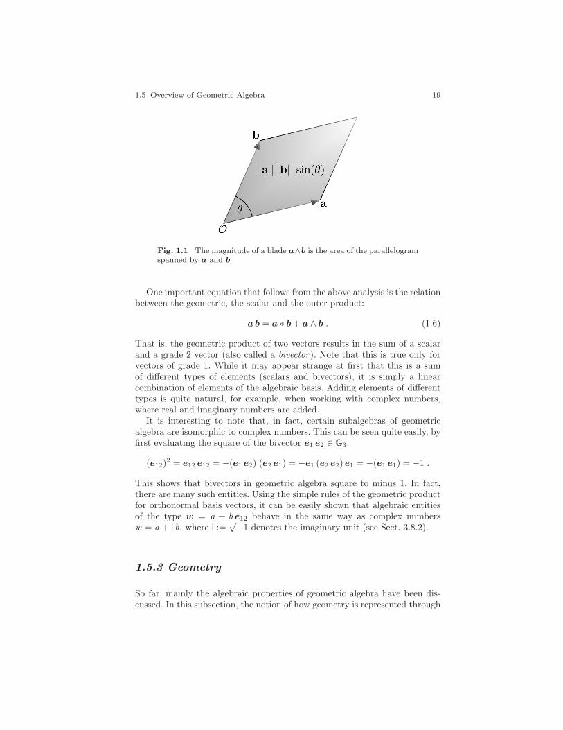
From the geometric interpretation of the dual, the geometric relation be-tween the vector cross product and the outer product can be deduced. Thevector cross product of a and b represents a vector perpendicular to thosetwo vectors. Hence, the outer product a ∧ b represents the plane spannedby a and b. It may actually be shown that with an appropriate definitionof the magnitude of multivectors, the magnitude ‖a ∧ b‖ is the area of theparallelogram spanned by a and b, as illustrated in Fig. 1.1 (see Sect. 4.1.1).

1.5 Overview of Geometric Algebra 19

Fig. 1.1 The magnitude of a blade a∧b is the area of the parallelogramspanned by a and b

One important equation that follows from the above analysis is the relationbetween the geometric, the scalar and the outer product:

ab = a ∗ b+ a ∧ b . (1.6)

That is, the geometric product of two vectors results in the sum of a scalarand a grade 2 vector (also called a bivector). Note that this is true only forvectors of grade 1. While it may appear strange at first that this is a sumof different types of elements (scalars and bivectors), it is simply a linearcombination of elements of the algebraic basis. Adding elements of differenttypes is quite natural, for example, when working with complex numbers,where real and imaginary numbers are added.

It is interesting to note that, in fact, certain subalgebras of geometricalgebra are isomorphic to complex numbers. This can be seen quite easily, byfirst evaluating the square of the bivector e1 e2 ∈ G3:

(e12)2 = e12 e12 = −(e1 e2) (e2 e1) = −e1 (e2 e2) e1 = −(e1 e1) = −1 .

This shows that bivectors in geometric algebra square to minus 1. In fact,there are many such entities. Using the simple rules of the geometric productfor orthonormal basis vectors, it can be easily shown that algebraic entitiesof the type w = a + b e12 behave in the same way as complex numbersw = a + i b, where i :=

√−1 denotes the imaginary unit (see Sect. 3.8.2).

1.5.3 Geometry

So far, mainly the algebraic properties of geometric algebra have been dis-cussed. In this subsection, the notion of how geometry is represented through

20 1 Introduction

algebraic entities is introduced. The basic idea is to associate an algebraicentity with the null space that it generates with respect to a particular oper-ation. One operation that is particularly useful for this purpose is the outerproduct; this stems from the fact that

x ∧ a = 0 ⇐⇒ x = u a , ∀ u ∈ R ,

where x,a ∈ R3. Similarly, it can be shown that for x,a, b ∈ R3,

x ∧ a ∧ b = 0 ⇐⇒ x = u a+ v b , ∀ u, v ∈ R .

In this way, a can be used to represent the line through the origin in thedirection of a and a ∧ b to represent the plane through the origin spannedby a and b. Later on in the text, this will be called the outer-product nullspace (see Sect. 3.2.2). This concept is extended in Chap. 4 to allow therepresentation of arbitrary lines, planes, circles, and spheres.

For example, in the geometric algebra of the projective space of R3, vectorsrepresent points in Euclidean space and the outer product of two vectorsrepresents the line passing through the points represented by those vectors.Similarly, the outer product of three vectors represents the plane through thethree corresponding points (see Sect. 4.2).

In the geometric algebra of conformal space, there exist two special points:the point at infinity, denoted by e∞, and the origin eo. Vectors in this spaceagain represent points in Euclidean space. However, the outer product oftwo vectors A and B, say, represents the corresponding point pair. The linethrough the points A and B is represented by A∧B∧e∞, that is, the entitythat passes through the points A and B and infinity. Furthermore, the outerproduct of three vectors represents the circle through the three correspondingpoints, and similarly for spheres (see Sect. 4.3).

Another important product that has not been mentioned yet is the in-ner product, denoted by ·. The inner product of two vectors a, b ∈ R3 isequivalent to the scalar product, i.e.

a · b = a ∗ b .

However, the inner product of a grade 1 and a grade 2 vector results in agrade 1 vector and not a scalar. That is, given three vectors a, b, c ∈ R3, then

x := a · (b ∧ c)

is a grade 1 vector. It is shown in Sect. 3.2.7 that this equation can beexpanded into

x = (a · b) c− (a · c) b = (a ∗ b) c− (a ∗ c) b .

Using this expansion, it is easy to verify that

1.5 Overview of Geometric Algebra 21

a ∗ x = 0 ⇐⇒ a ⊥ x ,

i.e. a is perpendicular to x. The geometric meaning of this property is thatthe inner product removes a linear subspace. That is, while the outer productcombines linear subspaces, the inner product subtracts them. Using theseoperations, a general intersection operation, the meet, can be defined (seeSect. 3.2.12). Using the meet, the intersection between any pair of geometricentities can be evaluated.

1.5.4 Transformations

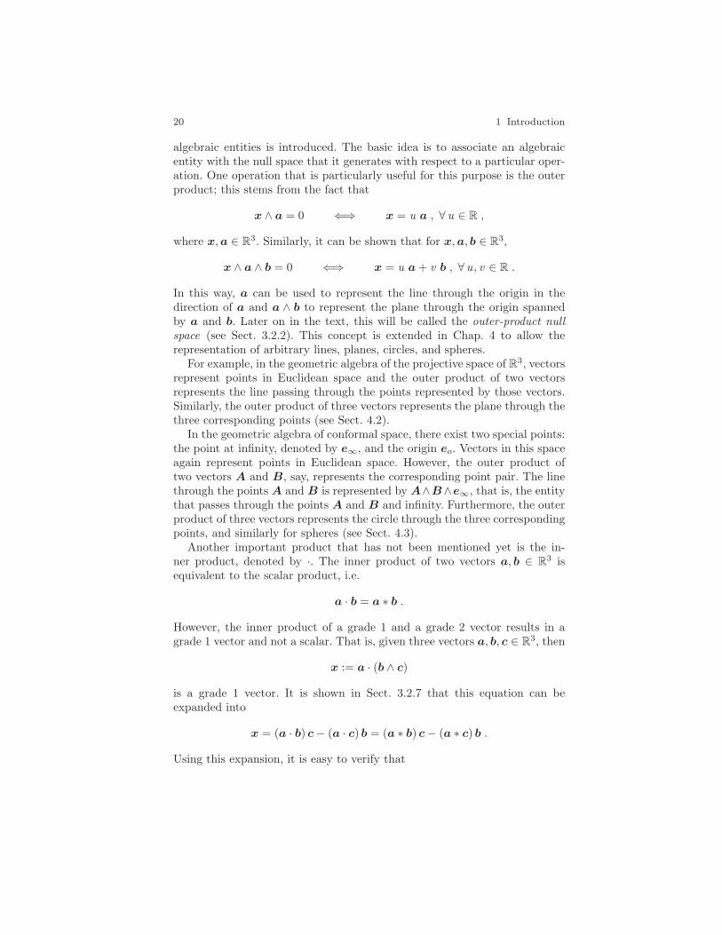
It was mentioned earlier that the fundamental transformation available ingeometric algebra is reflection. All other transformations, such as rotation,inversion, and translation, are represented through combinations of this basictransformation. In Sect. 3.3 it is shown that given vectors a,n ∈ R3, thevector

b := nan−1

is the reflection of a in n, as indicated in Fig. 1.2.

Fig. 1.2 Reflection of a in n

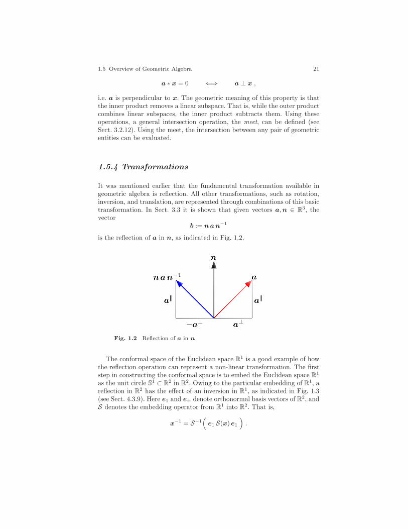
The conformal space of the Euclidean space R1 is a good example of howthe reflection operation can represent a non-linear transformation. The firststep in constructing the conformal space is to embed the Euclidean space R1

as the unit circle S1 ⊂ R2 in R2. Owing to the particular embedding of R1, areflection in R2 has the effect of an inversion in R1, as indicated in Fig. 1.3(see Sect. 4.3.9). Here e1 and e+ denote orthonormal basis vectors of R2, andS denotes the embedding operator from R1 into R2. That is,

x−1 = S−1(e1 S(x) e1

).

22 1 Introduction

Fig. 1.3 Reflection of S(x) in e1 represents inversion of x

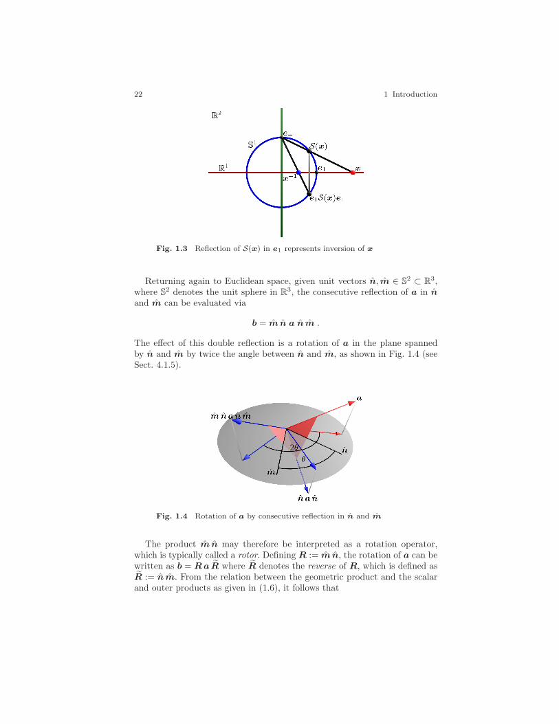
Returning again to Euclidean space, given unit vectors n, m ∈ S2 ⊂ R3,where S2 denotes the unit sphere in R3, the consecutive reflection of a in nand m can be evaluated via

b = m n a n m .

The effect of this double reflection is a rotation of a in the plane spannedby n and m by twice the angle between n and m, as shown in Fig. 1.4 (seeSect. 4.1.5).

Fig. 1.4 Rotation of a by consecutive reflection in n and m

The product m n may therefore be interpreted as a rotation operator,which is typically called a rotor. Defining R := m n, the rotation of a can bewritten as b = RaR where R denotes the reverse of R, which is defined asR := n m. From the relation between the geometric product and the scalarand outer products as given in (1.6), it follows that

1.5 Overview of Geometric Algebra 23

R = m n = m ∗ n+ m ∧ n = cos θ + sin θm ∧ n‖m ∧ n‖

, (1.7)

because ‖m ∧ n‖ = sin θ, if θ = ∠(m, n) (see Sect. 4.1.1). It was shownearlier that a bivector e1 e2, for example, squares to −1. The same is true forany unit bivector such as U := (m ∧ n)/‖m ∧ n‖, i.e. U2 = −1. IdentifyingU ∼= i, where i denotes the imaginary unit i =

√−1, it is clear that (1.7) can

be written as

cos θ + sin θ U ∼= cos θ + sin θ i = exp(θ i) .

Extending the definition of the exponential function to geometric algebra, itmay thus be shown that the rotor given in (1.7) can be written as

R = exp(θ U) .

Just as a rotation operator in Euclidean space is a combination of reflec-tions, the available transformations in conformal space are combinations ofinversions, which generates the group of conformal transformations. This in-cludes, for example, dilation and translation. Hence, rotors in the conformalembedding space can represent dilations and translations in the correspond-ing Euclidean space.

1.5.5 Outermorphism

The outermorphism property of transformation operators, not to be confusedwith an automorphism, plays a particularly important role, and is one of thereasons why geometric algebra is such a powerful language for the descrip-tion of geometry. The exact mathematical definition of the outermorphismof transformation operators is given in Sect. 3.3. The basic idea is as follows:if R denotes a rotor and a, b ∈ R3 are two vectors, then

R (a ∧ b) R = (RaR) ∧ (RbR) .

Since geometric entities are represented by the outer product of a numberof vectors, called a blade, the above equation implies that the rotation ofa blade is equivalent to the outer product of the rotation of the constituentvectors. That is, a rotor rotates any geometric entity, unlike rotation matrices,which differ for different geometric entities. Of course, all transformationoperators that are constructed from the geometric product of vectors satisfythe outermorphism property.