Applications of Conformal Geometric Algebra in Computer Vision and

Applications of Conformal Geometric Algebra inComputer Vision and Graphics

Rich Wareham, Jonathan Cameron, and Joan Lasenby

Cambridge University Engineering Department,Trumpington St., Cambridge, CB2 1PZ, United Kingdom

Abstract. This paper introduces the mathematical framework of con-formal geometric algebra (CGA) as a language for computer graphicsand computer vision. Specifically it discusses a new method for pose andposition interpolation based on CGA which firstly allows for existinginterpolation methods to be cleanly extended to pose and position in-terpolation, but also allows for this to be extended to higher-dimensionspaces and all conformal transforms (including dilations). In addition,we discuss a method of dealing with conics in CGA and the intersectionand reflections of rays with such conic surfaces. Possible applications forthese algorithms are also discussed.

1 Introduction

Since its inception in the mid-1970s, Computer Graphics (CG) has almost uni-versally used linear algebra as its mathematical framework. This may be dueto two factors; most early practitioners of computer graphics were mathemati-cians familiar with it and linear algebra provided a compact, efficient way ofrepresenting points, transformations, lines, etc.

As computing power becomes cheaper, the opportunity arises to investigatenew frameworks for CG which, although not providing the time/space efficiencyof linear algebra, may provide a conceptually simpler system or one of greateranalytical power.

We intend to introduce a system that makes use of Clifford Algebras andin particular the geometric interpretation introduced by [14], termed GeometricAlgebra. We then describe the use of this system for both pose and positioninterpolation and for the reflection and intersection of rays with conics.

1.1 Brief Overview of Geometric Algebra

We shall assume a basic familiarity with Clifford Algebras and merely describethe mechanism whereby they may be used to perform geometric operations.There already exist many introductions to Geometric Algebra that may be con-sulted [13, 9, 17].

We first write down a basis which can generate all elements of the CliffordAlgebra with vector elements in R

2 through linear combination

{1, e1, e2, e1e2} (1)

H. Li, P. J. Olver and G. Sommer (Eds.): IWMM 2004, LNCS 3519, pp. 329–349, 2005.c© Springer-Verlag Berlin Heidelberg 2005

330 R. Wareham, J. Cameron, and J. Lasenby

where e1, e2 are the usual orthonormal Euclidean basis vectors and hence e1e2 =e1 · e2 + e1 ∧ e2 = e1 ∧ e2. For convenience we shall denote eiej as eij and,generally, eiej . . . ek as eij...k. A general linear sum of these components is termeda multivector whereas a sum of only grade-n components is called a n-vector.This paper will use the convention of writing multivectors, bivectors, trivectorsand higher-grade elements in upper-case and vectors and scalars in lower-case.

Firstly, note that

(e1e2)2 = e1e2e1e2 = −e1e2e2e1 = −1 (2)

and thus we have an element of the algebra which squares to −1. As shown by[12, 9] this can be identified with the unit imaginary i =

√−1 in C and, as such,the highest-grade basis-element in a geometric algebra is often denoted I andreferred to as the pseudoscalar.

Note that in spaces with dimension n the maximum grade object possiblehas grade n and the n-vector e1 ∧ ...∧ en = I is therefore the pseudoscalar. Theresult of the product xI is termed the dual of x, denoted as x∗.

In [12] it was also shown that many of the identities and theorems dealingwith complex numbers have a direct analogue in Clifford Algebra. Therefore ageometrical interpretation, which was named Geometric Algebra, was suggested.

It can be shown [17, 14] that there is a general method for rotating a vectorx involving the formation of a multivector of the form R = e−Bφ/2. This rep-resents an anticlockwise rotation φ in a plane specified by the bivector B. Thetransformation is given by

x �→ RxR−1. (3)

We refer to these bivectors which have a rotational effect as rotors. The computa-tion of the inverse of a multivector is rather computationally intensive in general(and indeed can require a full 2n-dimension matrix inversion for a space of di-mension n). To combat this we define the reversion of a n-vector X = eiej ...ek

as X = ek...ejei, i.e. the literal reversion of the components. Since the reversionof eiej is ejei = −eiej , and by looking at the expression for R, it is clear thatR ≡ R−1 for rotors. Computing R is easier since it involves only a sign changefor some orthogonal elements of a multivector.

It is worth comparing this method of rotation to quaternions. The threebivectors B1 = e23, B2 = e31 and B3 = e12 act identically to the three imaginarycomponents of quaternions, i,−j and k respectively. The sign difference betweenB2 and j is due to the fact that the quaternions are not derived from the usualright-handed orthogonal co-ordinate system.

A particular rotation is represented via the quaternion q given by

q = q0 + q1i + q2j + q3k

where q20 +q2

1 +q22 +q2

3 = 1. Interpolation between rotations is then performedby interpolating each of the qi over the surface of a four-dimensional hyper-sphere. If we are interpolating between unit quaternions q0 and q1 the SLERPinterpolation is

Applications of Conformal Geometric Algebra 331

q ={

q0(q−10 q1)λ if q0 · q1 ≥ 0

q0(q−10 (−q1))λ otherwise

(4)

where λ varies in the range (0, 1) [19, 23].Recalling that, in complex numbers, the locus of exp(iφ

2 ) is the unit circle, itis somewhat simple to show that, for some bivector B, where B2 = −1, the locusof the action of exp(−B φ

2 ) upon a point with respect to varying φ is also a circlein the plane of B. Therefore if we consider some rotations R1, R2 = exp(kB)R1,where k is a scalar and B is some normalised bivector, it is easy to see aftersome thought that the quaternionic interpolation is exactly given by

Rλ = (R2R1)λR1 = exp(λkB)R1

where λ, the interpolation parameter, varies in the range (0, 1). A further mo-ment’s thought will reveal that this method, unlike quaternionic interpolation,is not confined to three dimensions but instead readily generalises to higher-dimensions.

Reflections. Reflections are particularly easy to represent in Geometric Alge-bra. Reflecting a vector a in a plane with unit normal n we obtain a reflectedvector a′ given by

a′ = −nan

which may easily be verified by expanding out to

a′ = a − 2(n · a)n

and noting that this does indeed give the reflection of a. This pattern of ‘sand-wiching’ an object between two others is often found in GA-based algorithmsand can be thought of as representing the reflection of the central object in the‘sandwiching’ object.

1.2 Conformal Geometric Algebra (CGA)

In the Conformal Model [14, 13, 18, 17, 20] we extend the space by adding twoadditional basis vectors. We first define the signature, (p, q) of a space A(p, q)with basis vectors, {ei}, such that e2

i = +1 for i = 1, ..., p and e2j = −1 for

j = p + 1, ..., p + q. For example R3 would be denoted as A(3, 0). We extend

A(3, 0) so that it becomes mixed signature and is defined by the basis

{e1, e2, e3, e, e}

where e and e are defined so that

e2 = 1, e2 = −1, e · e = 0

e · ei = e · ei = 0 ∀ i ∈ {1, 2, 3}.


This space is denoted as A(4, 1). In general a space A(p, q) is extended toA(p + 1, q + 1). We may now define the vectors n and n:

n = e + e, n = e − e

It is simple to show by direct substitution that both n and n are null vectors(i.e. n2 = n2 = 0). It can be shown [14, 17] that rigid body transforms may berepresented conveniently via rotors in this algebra.

We shall also make use of a transform based upon that proposed by Hestenesin [14]. The original transform is dimensionally inconsistent however so we in-troduce a fundamental unit length scale, λ, into the equation to make it dimen-sionally consistent

F (x) =1

2λ2

[x2n + 2λx − λ2n

] ≡ X (5)

where λ is usually set to be unity. At this point, notice that we can identify theorigin with n since F (0) ∝ n and that as x → ∞, F (x) becomes n. We may alsofind the inverse transform

F−1(X) = λ(X ∧ n) · e (6)

Rotations. As one might expect from their relation to complex numbers, thereexists an element of the algebra which performs rotation in the plane. Thesepure-rotation rotors all have the form e−B where B has only components of theform eij , i, j ∈ {1, 2, 3}.

A useful property of this mapping is that pure-rotation rotors retain theirproperties as can be shown by considering the effect of a rotor R = exp(−φ

2 eij),i, j ∈ {1, 2, 3} upon F (x). Setting λ = 1 for the moment,

RF (x)R =12R(x2n + 2x − n)R (7)

=12

(x2RnR + 2RxR − RnR

)= F (RxR) (8)

since rotors leave n and n invariant and (RxR)2 = x2.

Translations. The translation rotor Ta is defined [17, 18] as

Ta = exp[na

2

]= 1 +

na

2

and will transform a null-vector representation of the vector x to the null-vectorrepresentation of xa = x + a in the following manner:

F (xa) = TaF (x)Ta

Dilations. It can also be shown [17, 18] that the rotor Dα = exp(αee/2) hasthe effect of dilating x by a factor of e−α, i.e. DαF (x)Dα ∝ F (e−αx)


Table 1. Representations of various geometric objects

Line – L = X1 ∧ X2 ∧ n Circle – C = X1 ∧ X2 ∧ X3

Plane – Φ = X1 ∧ X2 ∧ X3 ∧ n Sphere – Σ = X1 ∧ X2 ∧ X3 ∧ X4

Inversions. Finally, inversions (x �→ x2/x) may be represented [17, 18] as F (x) �→eF (x)e. Although this will not be discussed here, this becomes particularly im-portant when considering non-Euclidean geometry.

This mapping has provided a similar advantage to that of homogeneous co-ordinates, namely that rigid body transforms become multiplicative and any suchtransform may be represented by a rotor. In addition, transforms followed by,or preceded by, a dilation or inversion may also be represented multiplicatively.

Representation of Geometric Objects. We have shown how rigid bodytransformations may be performed on a vector x by operating on its null-vectorrepresentation F (x). We may also ask what form the multivector M takes if thesolutions of F (x)∧M = 0 lie on a circle, sphere, line or plane. It has been shownin [17, 18] that the form of M depends only on the null-vector representationof points which lie on the object. The forms of M for various objects are sum-marised in Table 1. Note that if we identify the vector n with the point at infinity,a line is just a special case of a circle which passes through infinity and a planeis equally a special case of a sphere. It becomes convenient, therefore, to groupplanes and spheres by the collective term generalised spheres and, similarly, todefine a generalised circle as either a circle or a line.

Suppose we have a generalised sphere which passes through the points x1, · · · ,x4. Hence, for all points x on the object, F (x) ∧ M = 0 where

M = F (x1) ∧ F (x2) ∧ F (x3) ∧ F (x4). (9)

Now consider the effect of a rotor R upon M

RMR = RF (x1)R ∧ RF (x2)R ∧ RF (x3)R ∧ RF (x4)R (10)

as R(a ∧ b)R = R(a)R ∧ R(b)R. Furthermore we can say

RMR = F (Rx1R) ∧ F (Rx2R) ∧ F (Rx3R) ∧ F (Rx4R) (11)

which represents a generalised sphere passing through the transformed pointsYi = RXiR. Clearly, if R represents a conformal transformation, the generalisedsphere represented by M is similarly transformed.

Intersections may be performed efficiently using the meet operator. The gen-eral meet operation can be found by noting that for r-grade and s-grade bladesMr and Ms, a point, X, on the intersection must satisfy X ∧Mr = X ∧Ms = 0which can then be shown to be equivalent to

X ∧ [〈MrMs〉2l−r−s

]∗ = 0


where [ · ]∗ denotes multiplication by the pseudoscalar, l is the dimension of thespace (in the case of A(4, 1), l = 5) and 〈X〉i denotes the extraction of thei-grade component from X. If we define the meet operator

Mr ∨ Ms =[〈MrMs〉2l−r−s

]∗then we can interpret the meet of two objects as their intersection in many cases.

The key feature of this approach is that we have placed few constraints onthe form of Mr and Ms and thus we can intersect objects in a fairly generalmanner instead of using object-specific algorithms.

2 Pose and Position Interpolation

In this section we shall use the term displacement rotor to refer to a rotorwhich performs some rigid-body transform. Referring to the displacement rotorspresented above, we see that all of them have a common form; they are all ex-ponentiated bivectors. Rotations are generated by bivectors with no componentparallel to n and translations by a bivector with no components perpendicularto n. We may therefore postulate that all displacement rotors (we shall deal withrotors including a dilation later) can be expressed as

R = exp(B)

where B is the sum of two bivectors, one formed from the outer product oftwo vectors which have no components parallel to e or e. The other is formedfrom the outer product with n of vectors with no components parallel to e ore. The effect of this is to separate the basis bivectors of B into bivectors withcomponents of the form ei ∧ ej , ei ∧ e and ei ∧ e.

We shall proceed assuming that all displacement rotors can be written as theexponentiation of a bivector of the form B = ab+ cn where a, b and c are spatialvectors, i.e. if n ∈ A(m + 1, 1) then {a, b, c} ∈ R

m. It is clear that the set of allB is some linear subspace of all the bivectors.

We now suppose that we may interpolate rotors by defining some function�(R) which acts upon rotors to give the generating bivector element. We thenperform direct interpolation of this generator. We postulate that direct interpola-tion of such bivectors, as in the reformulation of quaternionic interpolation above,will give some smooth interpolation between the displacements. It is therefore adefining property of �(R) that

R ≡ exp(�(R)) (12)

and so �(R) may be considered to act as a logarithm-like function in this context.It is worth noting that �(R) does not possess all the properties usually associatedwith logarithms, notably that, since exp(A) exp(B) is not generally equal toexp(B) exp(A) in non-commuting algebras, �(exp(A) exp(B)) cannot be equalto A + B except in special cases.


To avoid the the risk of assigning more properties to �(R) than we haveshown, we shall resist the temptation to denote the function log(R). The mostobvious property of log(·) that �(·) doesn’t possess is log(AB) = log(A)+log(B).This is clear since the geometric product is not commutative in general whereasaddition is.

2.1 Form of exp(B) in Euclidean Space

The form of exp(B) may be derived after a little work. We start by assumingthat B is of the form B = φP + tn where t ∈ R

n, φ is some scalar and P is a2-blade where P 2 = −1 and it is formed from spatial vectors. We then definet‖ to be the component of t lying in the plane of P and t⊥ = t − t‖. From thisassumption it can be shown [26, 25] that the form of exp(B) is

exp(B) = [cos(φ) + sin(φ)P ] [1 + t⊥n] + sinc(φ)t‖n

It is also shown in [25] that this can only represent an Euclidean translationand rotation rotor. It is worth exploring the geometric interpretation of thisexpression. me vector satisfying a · n = a · P = 0.

In [25] we discuss how to obtain a geometrical description of the action ofthe rotor in terms of the bivector B. We shall state this here without proof. Westate that the action of the rotor

R = exp(

ψ

2P +

tn

2

)

is to translate along a vector t⊥ which is the component of t which does not liein the plane of P , rotate by ψ in the plane of P and finally translate along t′‖which is given by

t′‖ = −sinc(

ψ

2

)t‖

(cos

(ψ

2

)− sin

(ψ

2

)P

)

which is the component of t lying in the plane of P , rotated by ψ/2 in thatplane.

2.2 Method for Evaluating �(R)

We have found a form for exp(B) given that B is in a particular form. Nowwe seek a method to take an arbitrary displacement rotor, R = exp(B) and re-construct the original B. Should there exist a B for all possible R, we will showthat our initial assumption that all displacement rotors can be formed from asingle exponentiated bivector of special form is valid. We shall term this initialbivector the generator bivector (to draw a parallel with Lie algebras).

We can obtain the following identities for B = (ψ/2)P + tn/2 by simplyconsidering the grade of each component of the exponential:


〈R〉0 = cos(

ψ

2

)

〈R〉2 = sin(

ψ

2

)P + cos

(ψ

2

)t⊥n + sinc

(ψ

2

)t‖n

〈R〉4 = sin(

ψ

2

)Pt⊥n

It is somewhat straightforward to reconstruct ψ, t⊥ and t‖ from these com-ponents by partitioning a rotor as above. Once we have a method which givesthe generator B for any displacement rotor R we have validated our assumption.

Theorem 1. The inverse-exponential function �(R) is given by

�(R) = ab + c⊥n + c‖n

where

‖ab‖ =√

|(ab)2| = cos−1(〈R〉0)ab =

(〈R〉2 n) · esinc (‖ab‖)

c⊥n = − ab 〈R〉4‖ab‖2 sinc(‖ab‖)

c‖n = − ab 〈ab 〈R〉2〉2‖ab‖2 sinc(‖ab‖)

Proof. It is clear from the above that the form of ‖ab‖ is correct. We thus proceedto show the remaining equations to be true

〈R〉2 = cos(‖ab‖) c⊥n + sinc(‖ab‖) [ab + c‖n

]〈R〉2 n = sinc(‖ab‖) abn

(〈R〉2 n) · e = sinc(‖ab‖) ab

and hence the relation for ab is correct.

〈R〉4 = sinc(‖ab‖) abc⊥n

ab 〈R〉4 = −‖ab‖2 sinc(‖ab‖) c⊥n

and hence the relation for c⊥n is correct.

〈R〉2 = cos(‖ab‖) c⊥n + sinc(‖ab‖) [ab + c‖n

]ab 〈R〉2 = cos(‖ab‖) abc⊥n + sinc(‖ab‖)

[abc‖n − ‖ab‖2

]〈ab 〈R〉2〉2 = sinc(‖ab‖) abc‖n

and hence the relation for c‖n is correct.


3 Interpolation via Logarithms

We have shown that any displacement of Euclidean geometry may be mappedsmoothly onto a linear subspace of the bivectors. This immediately suggestsapplications to smooth interpolation of displacements. Consider a set of poseswe wish to interpolate, {P1, P2, ..., Pn} and a set of rotors which transform someorigin pose to these target poses, {R1, R2, ..., Rn}. We may map these rotorsonto the set of bivectors {�(R1), �(R2), ..., �(Rn)} which are simply points insome linear subspace of the bivectors. We may now choose any interpolation ofthese bivectors which lies in this space and for any bivector on the interpolant,B′

λ, we can compute a pose, exp(B′λ). We believe this method is more elegant

and conceptually simpler than many other approaches based on Lie-algebras[11, 21, 22, 5].

Another interpolation scheme is to have the poses defined by a set of chainedrotors so that {P1, P2, ..., Pn} is represented by

{R1,∆R1R1,∆R2R2, ...,∆RnRn}where Ri = ∆Ri−1Ri−1 as in figure 1. Using this scheme the interpolation

between pose Ri and Ri+1 involves forming the rotor Ri,λ = exp(Bi,λ)Ri−1

where Bi,λ = λ�(∆Ri−1) and λ varies between 0 and 1 giving Ri,0 = Ri−1 andRi,1 = Ri.

We now investigate two interpolation schemes which interpolate through tar-get poses, ensuring that each pose is passed through. This kind of interpolationis often required for key-frame animation techniques. The first form of inter-polation is piece-wise linear interpolation of the relative rotors (the latter caseabove). The second is direct quadratic interpolation of the bivectors representingthe final poses (the former case).

3.1 Piece-Wise Linear Interpolation

Direct piece-wise linear interpolation of the set of relative bivectors is one of thesimplest interpolation schemes we can consider. Consider the example shown infigure 1. Here there are three rotors to be interpolated. We firstly find a rotor,∆Rn which takes us from rotor Rn to the next in the interpolation sequence,Rn+1.

R1

∆R2∆R1

Origin

R2 = ∆R1R1

R3 = ∆R2∆R1R1

Fig. 1. Rotors used to piece-wise linearly interpolate between key-rotors


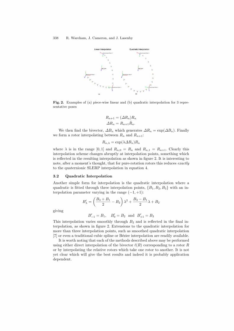
Fig. 2. Examples of (a) piece-wise linear and (b) quadratic interpolation for 3 repre-sentative poses

Rn+1 = (∆Rn)Rn

∆Rn = Rn+1Rn.

We then find the bivector, ∆Bn which generates ∆Rn = exp(∆Bn). Finallywe form a rotor interpolating between Rn and Rn+1:

Rn,λ = exp(λ∆Bn)Rn

where λ is in the range [0, 1] and Rn,0 = Rn and Rn,1 = Rn+1. Clearly thisinterpolation scheme changes abruptly at interpolation points, something whichis reflected in the resulting interpolation as shown in figure 2. It is interesting tonote, after a moment’s thought, that for pure-rotation rotors this reduces exactlyto the quaternionic SLERP interpolation in equation 4.

3.2 Quadratic Interpolation

Another simple form for interpolation is the quadratic interpolation where aquadratic is fitted through three interpolation points, {B1, B2, B3} with an in-terpolation parameter varying in the range (−1,+1):

B′λ =

(B3 + B1

2− B2

)λ2 +

B3 − B1

2λ + B2

givingB′

−1 = B1, B′0 = B2 and B′

+1 = B3

This interpolation varies smoothly through B2 and is reflected in the final in-terpolation, as shown in figure 2. Extensions to the quadratic interpolation formore than three interpolation points, such as smoothed quadratic interpolation[7] or even a traditional cubic spline or Bezier interpolation are readily available.

It is worth noting that each of the methods described above may be performedusing either direct interpolation of the bivector �(R) corresponding to a rotor Ror by interpolating the relative rotors which take one rotor to another. It is notyet clear which will give the best results and indeed it is probably applicationdependent.


3.3 Form of the Interpolation

We now derive a clearer picture of the precise form of a simple linear interpolationbetween two rotors in order to relate the interpolation to existing methods usedin mechanics and robotics. We will consider the method used above whereby therotor being interpolated takes one pose to another.

Path of the Linear Interpolation. Since we have shown that exp(B) is indeeda rotor, it follows that any Euclidean pure-translation rotor will commute withit. Thus we only need consider the interpolant path when interpolating fromthe origin to some other point since any other interpolation can be obtained bysimply translating the origin to the start point. This location independence ofthe interpolation is a desirable property in itself but also provides a powerfulanalysis mechanism.

We have identified in section 2.1 the action of the exp(B) rotor in terms ofψ,P, t‖ and t⊥. We now investigate the resulting interpolant path when interpo-lating from the origin. We shall consider the interpolant Rλ = exp(λB) where λis the interpolation co-ordinate and varies from 0 to 1. For any values of ψ,P, t‖and t⊥,

λB =λψ

2P +

λ(t⊥ + t‖)n2

from our expansion of exp(B) we see that the action of exp(λB) is a translationalong λt⊥, a rotation by λψ in the plane of P and finally a translation along

t′‖ = −sinc(

λψ

2

)λt‖

(cos

(λψ

2

)− sin

(λψ

2

)P

).

We firstly resolve a three dimensional orthonormal basis, {a, b, t⊥}, relativeto P where a and b are orthonormal vectors in the plane of P and hence P = ab.We may now express t‖ as t‖ = taa+ tbb where t{a,b} are suitably valued scalars.

The initial action of exp(B) upon a frame centred at the origin is therefore totranslate it to λt⊥ followed by a rotation in the plane of P . Due to our choice ofstarting point, this has no effect on the frame’s location (but will have an effecton the pose, see the next section).

Finally there is a translation along t′‖ which, using c = cos(

λψ2

)and s =

sin(

λψ2

), can be expressed in terms of a and b as

t′‖ = − 2s

λψλ(taa + tbb)(c − sab)

= −2s

ψ

[c(taa + tbb) + s(tba − tab)

]

≡ −2s

ψ

[a(tac + tbs) + b(tbc − tas)

].

The position, rλ, of the frame at λ along the interpolation is therefore

rλ = −2s

ψ(a(tac + tbs) + b(tbc − tas)) + λt⊥


which can easily be transformed via the harmonic addition theorem to

rλ = −2s

ψα

[a cos

(λψ

2+ β1

)+ b cos

(λψ

2+ β2

)]+ λt⊥

where α2 = (ta)2 + (tb)2, tan β1 = − tb

ta and tanβ2 = −−ta

tb . It is easy, viageometric construction or otherwise, to verify that this implies that β2 = β1 + π

2 .Hence cos(θ + β2) = − sin(θ + β1). We can now express the frame’s position as

rλ = −2α

ψ

[a sin

(λψ

2

)cos

(λψ

2+ β1

)− b sin

(λψ

2

)sin

(λψ

2+ β1

)]+ λt⊥

which can be re-arranged to give

rλ = −α

ψ[a (sin (λψ + β1) − sin β1) + b (cos (λψ + β1) − cos β1)] + λt⊥

= −α

ψ[a sin (λψ + β1) + b cos (λψ + β1)] +

α

ψ[a sin β1 + b cos β1] + λt⊥

noting that in the case ψ → 0, the expression becomes rλ = λt⊥ as one would ex-pect. Since a and b are defined to be orthonormal, the path is clearly some cylin-drical helix with the axis of rotation passing through α/ψ [a sin β1 + b cos β1].

It is worth noting a related result in screw theory, Chasles’ theorem [2],which states that a general displacement may be represented using a screw mo-tion (cylindrical helix) such as we have derived. Screw theory is widely usedin mechanics and robotics and the fact that the naıve linear interpolation gen-erated by this method is indeed a screw motion suggests that applications ofthis interpolation method may be wide-ranging, especially since this methodallows many other forms of interpolation, such as Bezier curves or three-pointquadratic to be performed with equal ease. Also the pure rotation interpolationgiven by this method reduces exactly to the quaternionic or Lie group interpola-tion result allowing the method to easily extend existing ones based upon theseinterpolations.

Pose of the Linear Interpolation. The pose of the transformed frame isunaffected by pure translation and hence the initial translation by λt⊥ has noeffect. The rotation by λψ in the plane, however, now becomes important. Thesubsequent translation along t′‖ also has no effect on the pose. We find, therefore,that the pose change λ along the interpolant is just the rotation rotor Rλψ,P .

3.4 Interpolation of Dilations

In certain circumstances it is desirable to add in the ability to interpolate dila-tions. It can be shown [6] that this can be done by extending the form of thebivector, B, which we exponentiate, as follows

B = φP + tn + ωN


where N = ee. This bivector form is now sufficiently general [6] to be ableto represent dilations as well. In this case obtaining the exponentiation andlogarithm function is somewhat involved [6]. We obtain finally that

exp(φP + tn + ωN)

= (cos(φ) + sin(φ)P ) (cosh(ω) + sinh(ω)N + sinhc(ω)t⊥n)

+(ω2 + φ2)−1[−ω sin(φ) cosh(ω) + φ cos(φ) sinh(ω)]P

+(ω2 + φ2)−1[ω cos(φ) sinh(ω) + φ sin(φ) cosh(ω)]t‖n

where sinhc(ω) = ω−1 sinh(ω). Note that this expression reduces to the originalform for exp(B) when ω = 0, as one would expect.

It is relatively easy to use the above expansion to derive a logarithm-likeinverse function.

If we let R = exp(B) then we may recreate B from R using the methodpresented below. Here we use 〈R|ei〉 to represent the component of R parallelto ei, i.e. 〈R|N〉 = 〈R|e45〉 in 3-dimensions. We also use 〈R〉i to represent thei-th grade-part of R and S(X) to represent the ‘spatial’ portion of X (i.e. thosecomponents not parallel to e and e).

ω = tanh−1(

〈R|N〉〈R|1〉

)

φ = cos−1(

〈R|N〉sinh(ω)

)

P = S(〈R〉2)sin(φ) cosh(ω)

t⊥ = − 〈R〉4−sin(φ) sinh(ω)PN

sin(φ)sinhc(ω)

(Pn2

)t = t‖ + t⊥

W = 〈R〉2 − cos(φ) sinh(ω)N− sin(φ) cosh(ω)P− cos(φ)sinhc(ω)t⊥n

X = −ω sin(φ) cosh(ω) + φ cos(φ) sinh(ω)

Z = ω cos(φ) sinh(ω) + φ sin(φ) cosh(ω)

t‖ = (−XP+Z)sin2(φ) cosh2(ω)+cos2(φ) sinh2(ω)

W

Path of Interpolation. We now consider the path resulting from the simplelinear interpolation of both pose and dilation using the results derived above.In [6] a full derivation is given and here we present only the result. As before,the derivation proceeds by considering the position, rλ, of the frame formed byapplying the interpolation rotor R = exp(λ(φP + tn + ωN)) to n (the origin),with the interpolation parameter λ varying from 0 to 1. After a little work weobtain the path of the interpolation as

rλ = − 1ω|t⊥|t⊥ − ω

ω2 + φ2|t‖|t‖ +

φ

ω2 + φ2|t‖|t � + e−2λω ·

⎛⎝ |t⊥|

ωt⊥ +

cos(2λφ + tan−1

(φω

))√

ω2 + φ2|t‖|t‖ −

sin(2λφ + tan−1

(φω

))√

ω2 + φ2|t‖|t �

⎞⎠

where t‖ is the normalised component of t parallel to P , t⊥ is the normalisedcomponent perpendicular to P and t � is a unit vector perpendicular to both t‖and t⊥. This is the equation of a conical helix.

It can be shown [6] that when setting the dilation component, ω, to zero thispath is equivalent to that derived for pose interpolation.


3.5 Applications

The method outlined is applicable to any problem which requires the smoothinterpolation of pose. We have chosen to illustrate an application in mesh defor-mation. Smooth mesh deformation is often required in medical imaging applica-tions [8] or video coding [15]. Here we use it to deform a 3d mesh in a mannerwhich has a visual effect similar to ‘grabbing’ a corner of the mesh and ‘twisting’it into place. We do this by specifying a set of ‘key-rotors’ which certain parts of

Fig. 3. A cube distorted via the linear interpolation of rotors specifying its cornervertices

Fig. 4. The Stanford Bunny[24] distorted by the same rotors


the mesh must rotate and translate to coincide with. Our implementation takesadvantage of the hardware acceleration offered by the Graphics Processing Units(GPUs) available on today’s consumer-level graphics hardware. A full discussionof the method will appear elsewhere.

We believe this method leads to images which are intuitively related to therotors specifying the deformation. Furthermore, the method need not only beapplied to meshes with simple geometry and can readily be applied to mesheswith complex geometry without any tears or other artifacts appearing in themesh. Figures 3 and 4 illustrate the method in the case of a cube and a meshwith approximately 36,000 vertices.

4 Conics

So far we have been limited in which objects we can manipulate and intersect inCGA. Specifically we can only deal with planes, circles, spheres, lines and points.In this section we consider a method of extending our approach to conics and in-tersections thereof. We shall proceed by considering the 3-dimensional Euclideancase but this method may be generalised to higher dimensions if required; herewe follow the procedure outlined in [16]. We shall begin by considering the setof points on the unit sphere at the origin:

{cθe1 + sθcφe2 + sθcφe3 : θ ∈ (0, 2π], φ ∈ (0, π]}where cθ = cos(θ), sθ = sin(θ) and similarly for sφ and cφ. We apply the trans-form F (·) to obtain the set, S, of representations for these points:

S ={n

2+ cθe1 + sθcφe2 + sθcφe3 − n

2: θ ∈ (0, 2π], φ ∈ (0, π]

}

and consider the effect of the transform from [16] below

Cα(X) = β[X +

α

2(X · e1) ∧ n

]

which we shall term the conic transform, upon the elements of S where β ischosen so that our normalisation constraint Cα(X) · n = −1 still holds:

{Cα(X) : X ∈ S}≡

{1

1 − α cos θ

(n

2+ cθe1 + sθcφe2 + sθcφe3

)− n

2: θ ∈ (0, 2π], φ ∈ (0, π]

}

The elements of this set are no-longer null-vectors (they have extra componentsparallel to n) but one may still apply the inverse mapping F−1(·) and extracta spatial vector (i.e. one with no components parallel to e or e). It is found[16, 6] that the spatial vectors extracted thus lie on the surface of a quadricwith a rotational cross-section corresponding to a conic. The form of this coniccross-section is determined by the parameter α which can be interpreted as theeccentricity:


– α = 0 : The set of points lie on the unit sphere.– 0 < α < 1 : The set of points lie on an ellipsoid formed by rotating an ellipse

in the e12 plane about e1. The origin lies at one of the foci and α is theeccentricity.

– α = 1 : The set of points lie on a paraboloid specified by the points

{x : 2x · e1 = [(x · e2)2 + (x · e3)2] − 1}.

– α > 1 : The set of points lie on a two-sheeted hyperboloid formed by rotatingan hyperbola in the e12 plane about e1. The origin is once again one of thefoci and the eccentricity is α.

We may therefore form a set of representations for points lying on these conicsby simply applying appropriate translation, dilation and rotation rotors afterthe conic transform.

4.1 Properties of the Conic Transform

It can further be shown [6] that the conic transform preserves the outer productbut not the inner (and hence geometric) products. That is to say Cα(X ∧ Y ) =Cα(X)∧Cα(Y ). It also preserves the ‘special’ vectors n and n. From this we caneasily show that Cα(·) does not change the nature of ‘flat’ objects (i.e. planesand lines transform to other planes and lines) since

Cα (X1 ∧ X2 ∧ · · · ∧ Xi ∧ n) = Cα(X1) ∧ Cα(X2) ∧ · · · ∧ Cα(Xi) ∧ Cα(n)= Cα(X1) ∧ Cα(X2) ∧ · · · ∧ Cα(Xi) ∧ n.

It is also easy to verify by direct substitution that the conic transform pre-serves direction of points from the origin, i.e. that

F−1(Cα(F (aiei))) =ai

1 − αa1ei

where we have adopted the usual summation convention.

4.2 Intersections

We may now consider how to apply this transform to intersecting conics withlines. Suppose that we have found a rotor R and value of α such that the set ofpoints represented by

{RCα(X)R : X ∈ S}lie on the conic we wish to intersect. Suppose further that we wish to intersect itwith the line represented by the trivector L (as in figure 5a). We shall denote thepoints of intersection A and B. Now consider the effect of applying C−1

α (RXR)to each of our objects and points (where X is the appropriate object). The pointson the conic are transformed to the unit sphere. The line, L, is transformed toC−1

α (RLR) (figure 5) which is still a line since the conic transform maps lines to


Fig. 5. Intersection of line L with (a) conic and (b) transformation back to intersectionwith unit sphere

lines. The points of intersection between this new line and our unit sphere maybe found via the usual meet formulation:

A′ ∧ B′ = Σ ∨ C−1α (RLR)

where Σ is the multivector representing the unit sphere which may be formedas

Σ = F (e1) ∧ F (e2) ∧ F (e3) ∧ F (−e1)

or similar.Finally we consider the transformed points A = RCα(A′)R and B = RCα(B′)·

R. They must lie upon our original line L since A′ and B′ clearly lie on C−1α (RLR)

andRCα(C−1

α (RLR))R = L.

They must also lie upon our conic since A′ and B′ lie on the unit sphere andthe transformation is exactly that which generated our original conic. If they lieupon our conic and upon L they must therefore be the points of intersection.We have therefore formulated a method for intersecting lines and conics.

4.3 Reflections

We now consider the reflection of rays from conics. In order to reflect a ray wewish to find the tangent plane for a conic at the intersection point of the incomingray with the conic. Again we make use of the fact that Cα(·) maps planes toplanes and apply C−1

α (RXR) to all objects moving the points on the conic tothe unit sphere. We then find the intersection point and tangent plane for theunit sphere. It can be shown [6] that when transformed back via RCα(·)R thetangent plane of the sphere maps to the tangent plane for the conic. Reflectioncan then be performed by simply reflecting the incoming ray L in this plane, Φ:

L′ = ΦLΦ.


5 Line Images in a Para-Catadioptric Camera

As an illustration of the power of the techniques described above, let us considerthe simple but useful question of what the image of a straight line in a parabolicmirror based Single View Point catadioptric (SVP Para-catadioptric) camera is.This problem has been considered in a number of papers e.g. [10, 27, 3, 4] and isuseful for calibration and scene reconstruction.

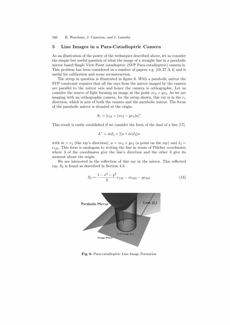
The setup in question is illustrated in figure 6. With a parabolic mirror theSVP constraint requires that all the rays from the mirror imaged by the cameraare parallel to the mirror axis and hence the camera is orthographic. Let usconsider the source of light forming an image at the point xe2 + ye3. As we areimaging with an orthographic camera, for the setup shown, this ray is in the e1

direction, which is axis of both the camera and the parabolic mirror. The focusof the parabolic mirror is situated at the origin.

S1 = [e23 + (xe3 − ye2)n]∗

This result is easily established if we consider the form of the dual of a line [17].

L∗ = mI3 + [(a ∧ m)I3]n

with m = e1 (the ray’s direction), a = xe2 + ye3 (a point on the ray) and I3 =e123. This form is analogous to writing the line in terms of Plucker coordinateswhere 3 of the coordinates give the line’s direction and the other 3 give itsmoment about the origin.

We are interested in the reflection of this ray in the mirror. This reflectedray, S2 is found as described in Section 4.3.

S2 =1 − x2 − y2

2e145 − xe245 − ye345 (13)

Fig. 6. Para-catadioptric Line Image Formation


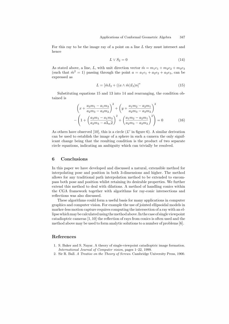
For this ray to be the image ray of a point on a line L they must intersect andhence

L ∨ S2 = 0 (14)

As stated above, a line, L, with unit direction vector m = m1e1 + m2e2 + m3e3

(such that m2 = 1) passing through the point a = a1e1 + a2e2 + a3e3, can beexpressed as

L = [mI3 + ((a ∧ m)I3)n]∗ (15)

Substituting equations 15 and 13 into 14 and rearranging, the condition ob-tained is

(x +

a3m1 − a1m3

a2m3 − a3m2

)2

+(

y +a1m2 − a2m1

a2m3 − a3m2

)2

−(

1 +(

a3m1 − a1m3

a2m3 − a3m2

)2

+(

a1m2 − a2m1

a2m3 − a3m2

)2)

= 0 (16)

As others have observed [10], this is a circle (L′ in figure 6). A similar derivationcan be used to establish the image of a sphere in such a camera the only signif-icant change being that the resulting condition is the product of two separatecircle equations, indicating an ambiguity which can trivially be resolved.

6 Conclusions

In this paper we have developed and discussed a natural, extensible method forinterpolating pose and position in both 3-dimensions and higher. The methodallows for any traditional path interpolation method to be extended to encom-pass both pose and position whilst retaining its desirable properties. We furtherextend this method to deal with dilations. A method of handling conics withinthe CGA framework together with algorithms for ray-conic intersections andreflections was also discussed.

These algorithms could form a useful basis for many applications in computergraphics and computer vision. For example the use of jointed ellipsoidal models inmarker-less motion capture requires computing the intersection of a ray with an el-lipsewhichmaybecalculatedusingthemethodabove. Inthecaseofsingleviewpointcatadioptric cameras [1, 10] the reflection of rays from conics is often used and themethod above may be used to form analytic solutions to a number of problems [6].

References

1. S. Baker and S. Nayar. A theory of single-viewpoint catadioptric image formation.International Journal of Computer vision, pages 1–22, 1999.

2. Sir R. Ball. A Treatise on the Theory of Screws. Cambridge University Press, 1900.


3. J. Barreto and H. Araujo. Paracatadioptric camera calibration using lines. In Pro-ceedings of ICCV, pages 1359–1365, 2003.

4. E. Bayro-Corrochano and C. Lopez-Franco. Omnidirectional vision: Unified modelusing conformal geometry. In Proceedings of ECCV, pages 536–548, 2004.

5. S. Buss and J. Fillmore. Spherical averages and applications to spherical splinesand interpolation. ACM Transactions on Graphics, pages 95–126, 2001.

6. J. Cameron. Applications of Geometric Algebra, August 2004. PhD First YearReport, Cambridge University Engineering Department.

7. Z. Cendes and S. Wong. C1 quadratic interpolation over arbitrary point sets. IEEEComputer Graphics and Applications, pages 8–16, Nov 1987.

8. S. Cotin, H. Delingette, and N. Ayache. Real-time elastic deformations of softtissues for surgery simulation. IEEE Transactions on Visualization and ComputerGraphics, 5(1):62–73, 1999.

9. C. Doran and A. Lasenby. Geometric Algebra for Physicists. CUP, 2003.10. C. Geyer and K. Daniilidis. Catadioptric projective geometry. International Jour-

nal of Computer Vision, pages 223–243, 2001.11. V. Govindu. Lie-algebraic averaging for globally consistent motion estimation. In

Proceedings of CVPR, pages 684–691, 2004.12. D. Hestenes. New Foundations for Classical Mechanics. Reidel, Second Edition,

1999.13. D. Hestenes. Old wine in new bottles: A new algebraic framework for computational

geometry. In E. Bayro-Corrochano and G. Sobczyk, editors, Geometric Algebra withApplications in Science and Engineering, chapter 1. Birkhauser, 2001.

14. D. Hestenes and G. Sobczyk. Clifford Algebra to Geometric Calculus: A unifiedlanguage for mathematics and physics. Reidel, 1984.

15. S. Kshirsagar, S. Garchery, and N. Magnenat-Thalmann. Feature point basedmesh deformation applied to mpeg-4 facial animation. In Proceedings of the IFIPTC5/WG5.10 DEFORM’2000 Workshop and AVATARS’2000 Workshop on De-formable Avatars, pages 24–34. Kluwer, 2001.

16. A. Lasenby. Recent applications of conformal geometric algebra. In InternationalWorkshop on Geometric Invariance and Applications in Engineering, Xi’an, China,May 2004.

17. J. Lasenby, A. Lasenby, and R. Wareham. A Covariant Approach to Geometry us-ing Geometric Algebra. Technical Report CUED/F-INFENG/TR-483, CambridgeUniversity Engineering Department, 2004.

18. H. Li, D. Hestenes, and A. Rockwood. Generalized homogeneous co-ordinates forcomputational geometry. In G. Sommer, editor, Geometric Computing with CliffordAlgebra, pages 25–58. Springer, 2001.

19. M. Lillholm, E.B. Dam, and M. Koch. Quaternions, interpolation and animation.Technical Report DIKU-TR-98/5, University of Copenhagen, July 1998.

20. S. Mann and L. Dorst. Geometric algebra: A computational framework for geo-metrical applications (part 2). IEEE Comput. Graph. Appl., 22(4):58–67, 2002.

21. M. Moakher. Means and averaging in the group of rotations. SIAM Journal ofApplied Matrix Analysis, pages 1–16, 2002.

22. F. Park and B. Ravani. Smooth invariant interpolation of rotations. ACM Trans-actions on Graphics, pages 277–295, 1997.

23. K. Shoemake. Animating rotation with quaternion curves. Computer Graphics,19(3):245–251, 1985.

24. G. Turk and M. Levoy. Zippered polygon meshes from range images. In SIG-GRAPH 1996 Proceedings, pages 331–318, 1994.


25. R. Wareham and J. Lasenby. Rigid body pose and position interpolation usinggeometric algebra. Submitted to ACM Transactions on Graphics, September 2004.

26. R. Wareham, J. Lasenby, and A. Lasenby. Computer Graphics using ConformalGeometric Algebra. Philosophical Transactions A of the Royal Society, special is-sue. To appear soon.

27. X. Ying and Z. Hu. Spherical objects based motion estimation for catadioptriccameras. In Proceedings of ICPR, pages 231–234, 2004.

Applications of Conformal Geometric Algebra in Computer Vision and

Documents

Transcript of Applications of Conformal Geometric Algebra in Computer Vision and