Reconstructing Binary Polygonal Objects From Projections ... · In many applications of tomography,...

This paper appeared in the journal CVGIP: Graphical Models and Image Processing, Vol. 56,No. 5, September, pp. 371–391, 1994.

Reconstructing Binary Polygonal Objects From Projections:

A Statistical View ∗

Peyman Milanfar(Corresponding Author)

SRI International333 Ravenswood AvenueMenlo Park, CA 94025

Phone: (617) 273-3388 extension 271E-mail: [email protected]

William C. KarlMultidimsional Signal Processing Laboratory

Department of Electrical and Computer EngineeringBoston University8 St Mary’s StreetBoston, MA 02215

Email: [email protected]

Alan S. WillskyLaboratory for Information and Decision Systems

Department of Electrical Engineering and Computer ScienceMassachusetts Institute of Technology

Cambridge, Massachusetts, 02139Email: [email protected]

∗This work was supported by the National Science Foundation under Grant 9015281-MIP, the Office of Naval Researchunder Grant N00014-91-J-1004, the US Army Research Office under Contract DAAL03-92-G-0115, and the Clement VaturiFellowship in Biomedical Imaging Sciences at MIT.

1

Report Documentation Page Form ApprovedOMB No. 0704-0188

Public reporting burden for the collection of information is estimated to average 1 hour per response, including the time for reviewing instructions, searching existing data sources, gathering andmaintaining the data needed, and completing and reviewing the collection of information. Send comments regarding this burden estimate or any other aspect of this collection of information,including suggestions for reducing this burden, to Washington Headquarters Services, Directorate for Information Operations and Reports, 1215 Jefferson Davis Highway, Suite 1204, ArlingtonVA 22202-4302. Respondents should be aware that notwithstanding any other provision of law, no person shall be subject to a penalty for failing to comply with a collection of information if itdoes not display a currently valid OMB control number.

1. REPORT DATE SEP 1994 2. REPORT TYPE

3. DATES COVERED 00-09-1994 to 00-09-1994

4. TITLE AND SUBTITLE Reconstructing Binary Polygonal Objects From Projections: A StatisticalView

5a. CONTRACT NUMBER

5b. GRANT NUMBER

5c. PROGRAM ELEMENT NUMBER

6. AUTHOR(S) 5d. PROJECT NUMBER

5e. TASK NUMBER

5f. WORK UNIT NUMBER

7. PERFORMING ORGANIZATION NAME(S) AND ADDRESS(ES) SRI International,333 Ravenswood Avenue,Menlo Park,CA,94025

8. PERFORMING ORGANIZATIONREPORT NUMBER

9. SPONSORING/MONITORING AGENCY NAME(S) AND ADDRESS(ES) 10. SPONSOR/MONITOR’S ACRONYM(S)

11. SPONSOR/MONITOR’S REPORT NUMBER(S)

12. DISTRIBUTION/AVAILABILITY STATEMENT Approved for public release; distribution unlimited

13. SUPPLEMENTARY NOTES

14. ABSTRACT

15. SUBJECT TERMS

16. SECURITY CLASSIFICATION OF: 17. LIMITATION OF ABSTRACT

18. NUMBEROF PAGES

34

19a. NAME OFRESPONSIBLE PERSON

a. REPORT unclassified

b. ABSTRACT unclassified

c. THIS PAGE unclassified

Standard Form 298 (Rev. 8-98) Prescribed by ANSI Std Z39-18

Abstract

In many applications of tomography, the fundamental quantities of interest in an image are geometric ones.In these instances, pixel based signal processing and reconstruction is at best inefficient, and at worst, non-robust in its use of the available tomographic data. Classical reconstruction techniques such as FilteredBack-Projection tend to produce spurious features when data is sparse and noisy; and these “ghosts” furthercomplicate the process of extracting what is often a limited number of rather simple geometric features. Inthis paper we present a framework that, in its most general form, is a statistically optimal technique forthe extraction of specific geometric features of objects directly from the noisy projection data. We focus onthe tomographic reconstruction of binary polygonal objects from sparse and noisy data. In our setting, thetomographic reconstruction problem is essentially formulated as a (finite dimensional) parameter estimationproblem. In particular, the vertices of binary polygons are used as their defining parameters. Under theassumption that the projection data are corrupted by Gaussian white noise, we use the Maximum Likelihood(ML) criterion, when the number of parameters is assumed known, and the Minimum Description Length(MDL) criterion for reconstruction when the number of parameters is not known. The resulting optimizationproblems are nonlinear and thus are plagued by numerous extraneous local extrema, making their solution farfrom trivial. In particular, proper initialization of any iterative technique is essential for good performance.To this end, we provide a novel method to construct a reliable yet simple initial guess for the solution. Thisprocedure is based on the estimated moments of the object, which may be conveniently obtained directlyfrom the noisy projection data.

2

List of Symbols

f(x, y) g(t, θ) O δ ω dx dy cos(θ) sin(θ) π

V i j m n σ Y Vml log∑

Vmap d VMDL N µ∫

R k H AR h T Vref L C Vinit det k tanI λ U E E z ‖ p ∗ infε % O u T v w α β zF A B a b

3

List of Figures

1 The Radon transform . . . . . . . . . . . . . . . . . . . . . . . . . . . . . . . . . . . . . . . . 62 A projection of a binary, polygonal object . . . . . . . . . . . . . . . . . . . . . . . . . . . . . 83 Illustration of Result 1 . . . . . . . . . . . . . . . . . . . . . . . . . . . . . . . . . . . . . . . . 144 Triangle example. SNR= 0 dB, 50 views, 20 samples/view: True(-), Reconstruction(- -).

%Error = 7.2 . . . . . . . . . . . . . . . . . . . . . . . . . . . . . . . . . . . . . . . . . . . . . 165 Hexagon example. SNR= 0 dB 50 views, 20 samples/view: True(-), Reconstruction(- -).

%Error=9.6 . . . . . . . . . . . . . . . . . . . . . . . . . . . . . . . . . . . . . . . . . . . . . . 176 From Top to Bottom: Sinograms with 50 projections and 20 samples per projection of I)

Noiseless Hexagon, II) Noisy data at 0 dB III) Reconstructed Hexagon. In each of theseimages, the horizontal axis is θ, the vertical axis is t, and the intensity values are the valuesof the corresponding projections mapped to the grayscale range of [0, 255] . . . . . . . . . . . 18

7 Sample reconstruction of a hexagon at 0 dB SNR using FBP: 64 views, 64 samples per view . 198 Sample reconstruction of a Hexagon at 0 dB SNR 64 views, 64 samples/view: True(-),

Reconstruction(- -) . . . . . . . . . . . . . . . . . . . . . . . . . . . . . . . . . . . . . . . . . 199 Mean performance curves for ML reconstructions of a triangle and a hexagon . . . . . . . . . 2010 Performance as a function of Number of Views . . . . . . . . . . . . . . . . . . . . . . . . . . 2011 Performance as a Function of Number of Samples per View . . . . . . . . . . . . . . . . . . . 2112 Cost vs number of sides for the hexagon in Figure 5 . . . . . . . . . . . . . . . . . . . . . . . 2213 Minimum MDL costs and Sample Reconstructions for an Ellipse . . . . . . . . . . . . . . . . 2214 True object (-), reconstruction (-.), initial guess (o) picked using Initial Guess Algorithm,

SNR= 4.35 dB. . . . . . . . . . . . . . . . . . . . . . . . . . . . . . . . . . . . . . . . . . . . . 2315 FBP Reconstruction of non-polygonal, non-convex Object: 3rd order Butterworth filter with

0.15 normalized cutoff frequency, SNR=4.35 dB . . . . . . . . . . . . . . . . . . . . . . . . . . 2416 MDL cost curve for the reconstruction of the kidney-shaped object with the Initial Guess

Algorithm used. . . . . . . . . . . . . . . . . . . . . . . . . . . . . . . . . . . . . . . . . . . . . 2417 A sample path of the reconstruction error at SNR=0 dB . . . . . . . . . . . . . . . . . . . . . 2518 Percent error for Hexagon vs SNR after outlier removal . . . . . . . . . . . . . . . . . . . . . 2619 A typical reconstruction at a local minimum with SNR= 0 dB . . . . . . . . . . . . . . . . . . 2720 A typical reconstruction at a local minimum with SNR= 4.35 dB . . . . . . . . . . . . . . . . 2721 Relative error in matching second order moments using the Initial Guess Algorithm . . . . . 32

4

1 Introduction

In many applications of tomography, the aim is to extract a rather small set of geometrically-based featuresfrom a given set of projection data [1, 2, 3]. In these instances, a full pixel-by-pixel reconstruction of theobject is a rather inefficient and non-robust approach. In addition, in many situations of practical interest,a full set of data with high signal-to-noise ratio (SNR) is often difficult, if not impossible, to obtain. Suchsituations arise in oceanography, nuclear medicine, surveillance, and non-destructive evaluation when due tothe geometry of the object or the imaging apparatus, only a few noisy projections are available [4, 5]. Inthese cases, the classical reconstruction techniques such as Filtered Back Projection (FBP) [5] and AlgebraicReconstruction Techniques (ART) fail to produce acceptable reconstructions. The shortcomings of theseclassical techniques in such situations can be attributed to two main sources. First, these techniques areinvariably aimed at reconstructing every pixel value of the underlying object with little regard to the qualityand quantity of the available data. To put it differently, there is no explicit or implicit mechanism to controlgreed and focus information, thus preventing one from attempting to extract more information from thedata than it actually contains. The second type of shortcoming results from the fact that if we assumethat the projection data are corrupted by Gaussian white noise, the process of reconstruction will havethe net effect of “coloring” this noise. This effect manifests itself in the object domain in the form ofspurious features which will complicate the detection of geometric features. This observation points out theimportance of working directly with the projection data when the final goal is the extraction of geometricinformation. In our effort to address these two issues, we have proposed the use of simple geometric priorsin the form of finitely parameterized objects (namely, binary polygonal). The assumption that the object tobe reconstructed is finitely parameterized allows for the tomographic reconstruction problem to be posed asa finite (relatively low-dimensional) parameter estimation problem. If we further assume, as we have donein the latter part of this paper, that the number of such parameters is also an unknown, we can formulatethe reconstruction problem as a Minimum Description Length estimation problem which provides for anautomatic (data-driven) method for computing the optimal parameterized objects with the “best” numberof parameters, given the data. This is, in essence, an information-theoretic criterion which gives us a directway to estimate as many parameters as the information content of the data allows us to, and thus controlthe greed factor.

Other efforts in the parametric/geometric study of tomographic reconstruction have been carried out inthe past. The work of Rossi and Willsky [6] and Prince and Willsky [7, 8, 9] has served as the startingpoint for this research effort. In the work of Rossi, the object was represented by a known profile, with onlythree geometric parameters; namely size, location, eccentricity, and orientation. These parameters were thenestimated from projection data using the Maximum Likelihood (ML) formulation. In their approach, thenumber of unknown parameters was fixed and the main focus of their work was on performance analysis.Prince, on the other hand, used a priori information such as prior probabilities on sinograms and consistencyconditions to compute Maximum A Posteriori (MAP) estimates of the sinogram and then used FBP toobtain a reconstruction. He made use of prior assumptions about shape, such as convexity, to reconstructconvex objects from support samples which were extracted from noisy projections through optimal filteringtechniques. The approach of Prince provided an explicit method for integrating geometric information intothe reconstruction process but was in essence still a pixel-by-pixel reconstruction. Extending these ideas, Lele,Kulkarni, and Willsky [10, 11] made use of only support information to produce polygonal reconstructions.Hanson [12] studied the reconstruction of axially symmetric objects from a single projection. Karl [13] alsohas studied the reconstruction of 3-D objects from two-dimensional silhouette projections.

The geometric modeling approach of Rossi and Willsky was expanded upon to include a more generalset of objects by Bresler, Macovski and Fessler [14, 15, 16, 17]. In these papers, the authors chose sequencesof 3-D cylinders and ellipsoids parameterized by stochastic dynamic models based on their radius, position,and orientation to model and reconstruct objects in two and three dimensions from projections.

Recently, Thirion [2] has introduced a technique to extract boundaries of objects from raw tomographicdata through edge detection in the sinogram. Other work in geometric reconstruction by Chang [18] and morerecently Kuba, Volcic, Gardner and Fishburn, [19, 20, 21, 22] has been concerned with the reconstruction ofbinary objects from only two noise-free projections.

Our approach provides a statistically optimal ML formulation for the direct recovery of vertices of binary

5

f(x,y)

X

t

θ

g( , )t θ

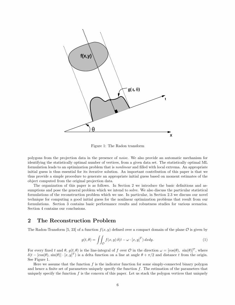
Figure 1: The Radon transform

polygons from the projection data in the presence of noise. We also provide an automatic mechanism foridentifying the statistically optimal number of vertices, from a given data set. The statistically optimal MLformulation leads to an optimization problem that is nonlinear and filled with local extrema. An appropriateinitial guess is thus essential for its iterative solution. An important contribution of this paper is that wethus provide a simple procedure to generate an appropriate initial guess based on moment estimates of theobject computed from the original projection data.

The organization of this paper is as follows. In Section 2 we introduce the basic definitions and as-sumptions and pose the general problem which we intend to solve. We also discuss the particular statisticalformulations of the reconstruction problem which we use. In particular, in Section 2.3 we discuss our noveltechnique for computing a good initial guess for the nonlinear optimization problems that result from ourformulations. Section 3 contains basic performance results and robustness studies for various scenarios.Section 4 contains our conclusions.

2 The Reconstruction Problem

The Radon-Transform [5, 23] of a function f(x, y) defined over a compact domain of the plane O is given by

g(t, θ) =∫ ∫Of(x, y) δ(t− ω · [x, y]T ) dxdy. (1)

For every fixed t and θ, g(t, θ) is the line-integral of f over O in the direction ω = [cos(θ), sin(θ)]T , whereδ(t − [cos(θ), sin(θ)] · [x, y]T ) is a delta function on a line at angle θ + π/2 and distance t from the origin.See Figure 1.

Here we assume that the function f is the indicator function for some simply-connected binary polygonand hence a finite set of parameters uniquely specify the function f . The estimation of the parameters thatuniquely specify the function f is the concern of this paper. Let us stack the polygon vertices that uniquely

6

define f in a vector V . We will assume throughout that the data available to us are discrete samples ofg which are corrupted by Gaussian white noise of known intensity. In particular, our observations will begiven by

Yi,j = g(ti, θj, V ∗) + w(ti, θj), (2)

for 1 ≤ i ≤ m, 1 ≤ j ≤ n where V ∗ is the true object we wish to reconstruct. The variables w(ti, θj) areassumed to be independent, identically distributed (i.i.d.) Gaussian random variables with variance σ2. Wewill denote by Y the vector of all such observations.

2.1 Maximum Likelihood Approach

In our approach, the original data in (2) are used to directly estimate the vertices V of a polygon in astatistically optimal way. The dimension of the parameter vector V (i.e. the number of sides) is determinedby the level of detail that one can extract from the sparse and noisy data. For clarity, we first consider thecase where a fixed and known number of vertices is assumed. In this case, the Maximum Likelihood (ML)[24] estimate, Vml, of the parameter vector V is given by that value of V which makes the observed datamost likely. In particular, using the monotonicity of the logarithm:

Vml = arg maxV

log [P (Y |V )] , (3)

where P (Y |V ) denotes the conditional probability density of the observed data set Y given the parametervector V . It is well-known that given the assumption that the data is corrupted by i.i.d. Gaussian randomnoise, the solution to the above ML-estimation problem is precisely equivalent to the following NonlinearLeast Squares Error (NLSE) formulation

Vml = arg minV

∑i,j

‖Yi,j − g(ti, θj , V )‖2. (4)

The formulation (4) shows that, in contrast to the linear formulation of classical reconstruction algorithms,the ML tomographic reconstruction approach, while yielding an optimal reconstruction framework, generallyresults in a highly nonlinear minimization problem. It is the nature of the dependence of g on the parametervector V that makes the problem nonlinear.

Finally, note that if additional explicit geometric information is available in terms of a prior probabilisticdescription of the object vector V , then a Maximum-A-Posteriori estimate of V may be computed as follows:

Vmap = arg maxV

log [P (V |Y )] (5)

In this work we concentrate on the ML problem given in (3) and its extensions, though application of ourresults to the MAP formulation is straightforward.

2.2 Minimum Description Length

In the previous ML discussion we assumed we had prior knowledge of the number of parameters describingthe underlying object. Without this knowledge, we can consider the Minimum Description Length (MDL)principal [25]. In this approach, the cost function is formulated such that the global minimum of the costcorresponds to a model of least order that explains the data best. The MDL approach in essence extends theMaximum Likelihood principal by including a term in the optimization criterion that measures the modelcomplexity. In the present context, the model complexity refers to the number of vertices used to capturethe object in question. Whereas the ML approach maximizes the log likelihood function given in (3), theMDL criterion maximizes a modified log likelihood function, as follows:

VMDL = arg maxV,N

{log [P (Y |V )]− N

2log(d)

}, (6)

where d = mn is the number of samples of g(t, θ) and N refers to the number of parameters defining thereconstruction. Roughly speaking, the MDL cost is proportional to the number of bits required to model

7

V

V

V

V

V

1

2

3

4

5

t t t t t1 2 3 4 5

=[x ,y ]2

T2

Figure 2: A projection of a binary, polygonal object

the observed data set with a model of order N , hence the term Minimum Description Length. Under ourassumed observation model (2) the MDL criterion (6) yields the following nonlinear optimization problemfor the optimal parameter vector VMDL:

VMDL = arg minN

minV{σ−2

∑i,j

‖Yi,j − g(ti, θj , V )‖2 +N log(d)}, (7)

where the optimization is now performed over both V and the number of parameters N . Note that thesolution of the inner minimization in (7) essentially requires solution of the original ML problem (3) or (4)for a sequence of values of N .

Unless otherwise stated, we assume from here on that the matrix V contains the vertices of an N -sidedbinary, polygonal region as follows:

V =[V1 V2 · · · VN

], (8)

where Vi = [xi, yi]T denote the Cartesian coordinates of the ith vertex of the polygonal region arranged inthe counter-clockwise direction (See Figure 2). Note that we use a matrix of parameters rather than a vectorin what follows for notational convenience in the algorithms to follow, though this is not essential.

2.3 Algorithmic Aspects – Computing A Good Initial Guess

Given the highly nonlinear nature of the dependence of the cost function in (4) on the parameters in V , itappears evident that given a poor initial condition, typical numerical optimization algorithms may convergeto local minima of the cost function. Indeed, this issue is a major obstacle to the use of a statistically optimal,though nonlinear, approach such as given in (3) or (6). In this section we describe a method for using theprojection data to directly compute an initial guess that is sufficiently close to the true global minimum asto, on average, result in convergence to it, or to a local minimum nearby. We do this by estimating themoments of the object directly from the projection data and then using (some of) these moments to computean initial guess.

In considering the use of moments as the basis for an initialization algorithm, one is faced with twoimportant issues. The first is that although estimating the moments of a function from its projections is

8

a relatively easy task, as we have shown in [26, 27], the reconstruction of a function from a finite numberof moments is in general a highly ill-posed problem even when these moments are exactly known [28].Furthermore, in our framework the moments are estimated from noisy data, and hence are themselves noisy.In fact, as higher and higher order moments are estimated, the error in the estimates of these momentsbecomes larger. Our approach avoids these moment related difficulties by using the moments only to guidean initial coarse estimate of the object parameters for subsequent use in solution of the nonlinear ML or MDLproblems. This initial estimate, in turn, itself mitigates the difficulties associated with the nonlinearities ofthe optimal statistical approaches. In particular, the amount of computation involved in arriving at aninitial guess using our moment-based method is far smaller than the amount of computation (number ofiterations) required to converge to an answer given a poor initial guess, especially since a poor initial guessmay converge to a local minimum far from the basin of the global minimum. Further, the parameterizationof the objects serves to regularize and robustify the moment inversion process [28, 29, 30, 31].

Our method of using moments to generate an initial guess is based on the following set of observations.First, let µpq, 0 ≤ p, q denote the moment of f(x, y) of order p+ q as given by:

µpq =∫ ∫

xpyqf(x, y) dx dy (9)

In particular, note that the moments up to order 2 have the following physical relationships. The zerothorder moment µ00 is the area of the object, the first order moments µ01 and µ10 are the coordinates of thecenter of mass of the object scaled by the area, and the second order moments µ02, µ11, µ20 are used to formthe entries of the inertia matrix of the object. Thus these moments contain basic geometric informationabout object size, location, and elongation and orientation that, if available, could be used to guide ourinitialization of the nonlinear optimization problems (4) or (7). Our first aim then is to estimate themdirectly from the noisy projection data. To that end, it is easy to show that [23]:∫ ∞

−∞g(t, θ) tk dt =

∫ ∫R2f(x, y) [x cos(θ) + y sin(θ)]k dx dy. (10)

By expanding the integrand on the right hand side of (10), it becomes apparent that the moments of theprojections are linearly related to the moments µpq of the object. In particular, specializing (10) to k = 0, 1, 2,and noting that f(x, y) is an indicator function when the objects in question are binary, we arrive at thefollowing relationships between µpq, 0 ≤ p+ q ≤ 2 and the projection g(t, θ) of f(x, y) at each angle θ:

µ00 =∫g(t, θ) dt ≡ H(0)(θ) (11)

[cos(θ) sin(θ)

] [ µ10

µ01

]=

∫g(t, θ) t dt ≡ H(1)(θ) (12)

[cos2(θ) 2 sin(θ) cos(θ) sin2(θ)

] µ20

µ11

µ02

=∫g(t, θ) t2 dt ≡ H(2)(θ) (13)

Thus if we have projections at three or more distinct, known angles we can estimate the moments of up toorder 2 of the object we wish to reconstruct. The computation of these moments is a linear calculation,making their estimation from projections straightforward (see [26]). Since, in general, many more than threeprojections are available, the estimation of these moments determining the area, center, and inertia axes ofthe object is overdetermined. The result is a robustness to noise and data sparsity through a reduction inthe noise variance of their estimated values. In particular, we can stack the moments H(k)(θj) obtained fromthe projections at each angle θj to arrive at the following overall equations for the µpq up to order 2: 1

...1

µ00 =

H(0)(θ1)

...H(0)(θn)

(14)

9

cos(θ1) sin(θ1)...

...cos(θn) sin(θn)

[ µ10

µ01

]=

H(1)(θ1)

...H(1)(θn)

(15)

cos2(θ1) 2 sin(θ1) cos(θ1) sin2(θ1)...

......

cos2(θn) 2 sin(θn) cos(θn) sin2(θn)

µ20

µ11

µ02

=

H(2)(θ1)

...H(2)(θn)

(16)

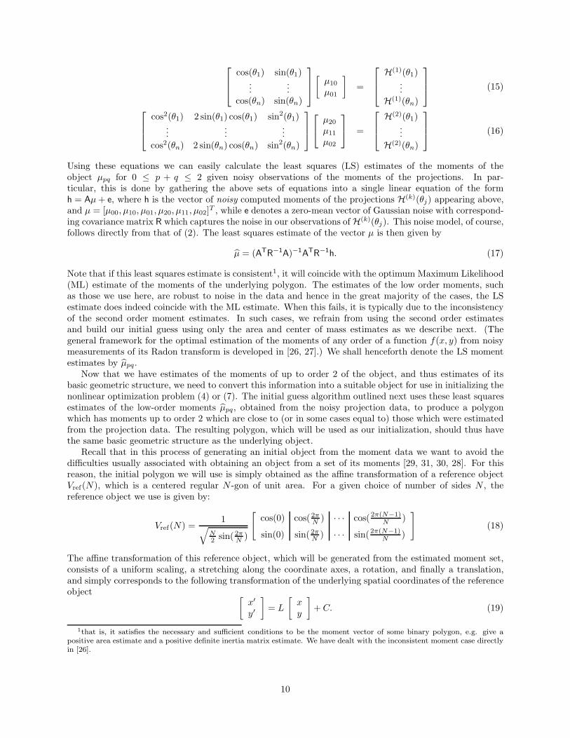
Using these equations we can easily calculate the least squares (LS) estimates of the moments of theobject µpq for 0 ≤ p + q ≤ 2 given noisy observations of the moments of the projections. In par-ticular, this is done by gathering the above sets of equations into a single linear equation of the formh = Aµ+ e, where h is the vector of noisy computed moments of the projections H(k)(θj) appearing above,and µ = [µ00, µ10, µ01, µ20, µ11, µ02]T , while e denotes a zero-mean vector of Gaussian noise with correspond-ing covariance matrix R which captures the noise in our observations of H(k)(θj). This noise model, of course,follows directly from that of (2). The least squares estimate of the vector µ is then given by

µ = (ATR−1A)−1ATR−1h. (17)

Note that if this least squares estimate is consistent1, it will coincide with the optimum Maximum Likelihood(ML) estimate of the moments of the underlying polygon. The estimates of the low order moments, suchas those we use here, are robust to noise in the data and hence in the great majority of the cases, the LSestimate does indeed coincide with the ML estimate. When this fails, it is typically due to the inconsistencyof the second order moment estimates. In such cases, we refrain from using the second order estimatesand build our initial guess using only the area and center of mass estimates as we describe next. (Thegeneral framework for the optimal estimation of the moments of any order of a function f(x, y) from noisymeasurements of its Radon transform is developed in [26, 27].) We shall henceforth denote the LS momentestimates by µpq.

Now that we have estimates of the moments of up to order 2 of the object, and thus estimates of itsbasic geometric structure, we need to convert this information into a suitable object for use in initializing thenonlinear optimization problem (4) or (7). The initial guess algorithm outlined next uses these least squaresestimates of the low-order moments µpq, obtained from the noisy projection data, to produce a polygonwhich has moments up to order 2 which are close to (or in some cases equal to) those which were estimatedfrom the projection data. The resulting polygon, which will be used as our initialization, should thus havethe same basic geometric structure as the underlying object.

Recall that in this process of generating an initial object from the moment data we want to avoid thedifficulties usually associated with obtaining an object from a set of its moments [29, 31, 30, 28]. For thisreason, the initial polygon we will use is simply obtained as the affine transformation of a reference objectVref(N), which is a centered regular N -gon of unit area. For a given choice of number of sides N , thereference object we use is given by:

Vref(N) =1√

N2 sin(2π

N )

[cos(0) cos(2π

N ) · · · cos(2π(N−1)N )

sin(0) sin(2πN ) · · · sin(2π(N−1)

N )

](18)

The affine transformation of this reference object, which will be generated from the estimated moment set,consists of a uniform scaling, a stretching along the coordinate axes, a rotation, and finally a translation,and simply corresponds to the following transformation of the underlying spatial coordinates of the referenceobject [

x′

y′

]= L

[xy

]+ C. (19)

1that is, it satisfies the necessary and sufficient conditions to be the moment vector of some binary polygon, e.g. give apositive area estimate and a positive definite inertia matrix estimate. We have dealt with the inconsistent moment case directlyin [26].

10

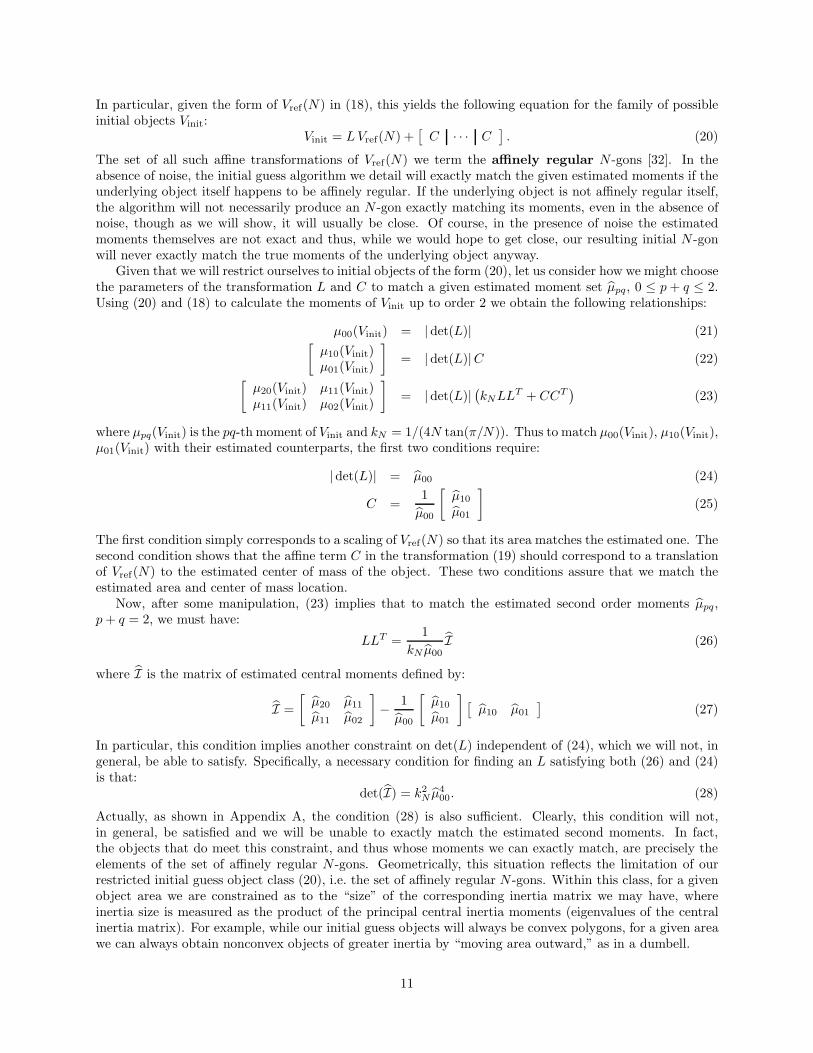
In particular, given the form of Vref(N) in (18), this yields the following equation for the family of possibleinitial objects Vinit:

Vinit = LVref(N) +[C · · · C

]. (20)

The set of all such affine transformations of Vref(N) we term the affinely regular N -gons [32]. In theabsence of noise, the initial guess algorithm we detail will exactly match the given estimated moments if theunderlying object itself happens to be affinely regular. If the underlying object is not affinely regular itself,the algorithm will not necessarily produce an N -gon exactly matching its moments, even in the absence ofnoise, though as we will show, it will usually be close. Of course, in the presence of noise the estimatedmoments themselves are not exact and thus, while we would hope to get close, our resulting initial N -gonwill never exactly match the true moments of the underlying object anyway.

Given that we will restrict ourselves to initial objects of the form (20), let us consider how we might choosethe parameters of the transformation L and C to match a given estimated moment set µpq, 0 ≤ p+ q ≤ 2.Using (20) and (18) to calculate the moments of Vinit up to order 2 we obtain the following relationships:

µ00(Vinit) = |det(L)| (21)[µ10(Vinit)µ01(Vinit)

]= |det(L)|C (22)[

µ20(Vinit) µ11(Vinit)µ11(Vinit) µ02(Vinit)

]= |det(L)|

(kNLL

T + CCT)

(23)

where µpq(Vinit) is the pq-th moment of Vinit and kN = 1/(4N tan(π/N)). Thus to match µ00(Vinit), µ10(Vinit),µ01(Vinit) with their estimated counterparts, the first two conditions require:

|det(L)| = µ00 (24)

C =1µ00

[µ10

µ01

](25)

The first condition simply corresponds to a scaling of Vref(N) so that its area matches the estimated one. Thesecond condition shows that the affine term C in the transformation (19) should correspond to a translationof Vref(N) to the estimated center of mass of the object. These two conditions assure that we match theestimated area and center of mass location.

Now, after some manipulation, (23) implies that to match the estimated second order moments µpq,p+ q = 2, we must have:

LLT =1

kN µ00I (26)

where I is the matrix of estimated central moments defined by:

I =[µ20 µ11

µ11 µ02

]− 1µ00

[µ10

µ01

] [µ10 µ01

](27)

In particular, this condition implies another constraint on det(L) independent of (24), which we will not, ingeneral, be able to satisfy. Specifically, a necessary condition for finding an L satisfying both (26) and (24)is that:

det(I) = k2N µ

400. (28)

Actually, as shown in Appendix A, the condition (28) is also sufficient. Clearly, this condition will not,in general, be satisfied and we will be unable to exactly match the estimated second moments. In fact,the objects that do meet this constraint, and thus whose moments we can exactly match, are precisely theelements of the set of affinely regular N -gons. Geometrically, this situation reflects the limitation of ourrestricted initial guess object class (20), i.e. the set of affinely regular N -gons. Within this class, for a givenobject area we are constrained as to the “size” of the corresponding inertia matrix we may have, whereinertia size is measured as the product of the principal central inertia moments (eigenvalues of the centralinertia matrix). For example, while our initial guess objects will always be convex polygons, for a given areawe can always obtain nonconvex objects of greater inertia by “moving area outward,” as in a dumbell.

11

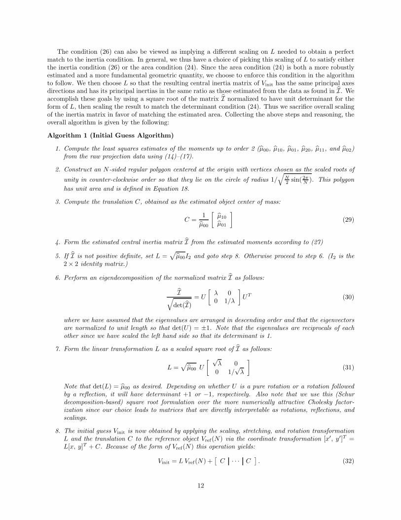
The condition (26) can also be viewed as implying a different scaling on L needed to obtain a perfectmatch to the inertia condition. In general, we thus have a choice of picking this scaling of L to satisfy eitherthe inertia condition (26) or the area condition (24). Since the area condition (24) is both a more robustlyestimated and a more fundamental geometric quantity, we choose to enforce this condition in the algorithmto follow. We then choose L so that the resulting central inertia matrix of Vinit has the same principal axesdirections and has its principal inertias in the same ratio as those estimated from the data as found in I. Weaccomplish these goals by using a square root of the matrix I normalized to have unit determinant for theform of L, then scaling the result to match the determinant condition (24). Thus we sacrifice overall scalingof the inertia matrix in favor of matching the estimated area. Collecting the above steps and reasoning, theoverall algorithm is given by the following:

Algorithm 1 (Initial Guess Algorithm)

1. Compute the least squares estimates of the moments up to order 2 (µ00, µ10, µ01, µ20, µ11, and µ02)from the raw projection data using (14)–(17).

2. Construct an N -sided regular polygon centered at the origin with vertices chosen as the scaled roots of

unity in counter-clockwise order so that they lie on the circle of radius 1/√

N2 sin(2π

N ). This polygonhas unit area and is defined in Equation 18.

3. Compute the translation C, obtained as the estimated object center of mass:

C =1µ00

[µ10

µ01

](29)

4. Form the estimated central inertia matrix I from the estimated moments according to (27)

5. If I is not positive definite, set L =√µ00I2 and goto step 8. Otherwise proceed to step 6. (I2 is the

2× 2 identity matrix.)

6. Perform an eigendecomposition of the normalized matrix I as follows:

I√det(I)

= U

[λ 00 1/λ

]UT (30)

where we have assumed that the eigenvalues are arranged in descending order and that the eigenvectorsare normalized to unit length so that det(U) = ±1. Note that the eigenvalues are reciprocals of eachother since we have scaled the left hand side so that its determinant is 1.

7. Form the linear transformation L as a scaled square root of I as follows:

L =√µ00 U

[ √λ 0

0 1/√λ

](31)

Note that det(L) = µ00 as desired. Depending on whether U is a pure rotation or a rotation followedby a reflection, it will have determinant +1 or −1, respectively. Also note that we use this (Schurdecomposition-based) square root formulation over the more numerically attractive Cholesky factor-ization since our choice leads to matrices that are directly interpretable as rotations, reflections, andscalings.

8. The initial guess Vinit is now obtained by applying the scaling, stretching, and rotation transformationL and the translation C to the reference object Vref(N) via the coordinate transformation [x′, y′]T =L[x, y]T + C. Because of the form of Vref(N) this operation yields:

Vinit = L Vref(N) +[C · · · C

]. (32)

12

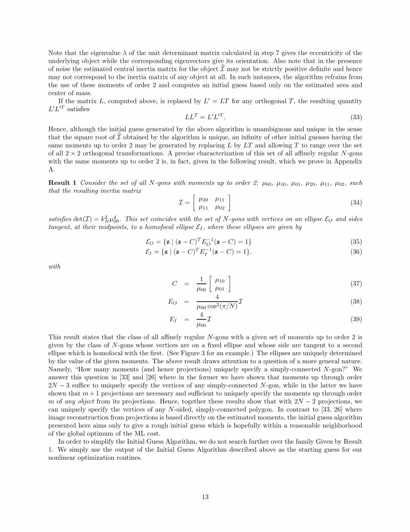
Note that the eigenvalue λ of the unit determinant matrix calculated in step 7 gives the eccentricity of theunderlying object while the corresponding eigenvectors give its orientation. Also note that in the presenceof noise the estimated central inertia matrix for the object I may not be strictly positive definite and hencemay not correspond to the inertia matrix of any object at all. In such instances, the algorithm refrains fromthe use of these moments of order 2 and computes an initial guess based only on the estimated area andcenter of mass.

If the matrix L, computed above, is replaced by L′ = LT for any orthogonal T , the resulting quantityL′L′T satisfies

LLT = L′L′T . (33)

Hence, although the initial guess generated by the above algorithm is unambiguous and unique in the sensethat the square root of I obtained by the algorithm is unique, an infinity of other initial guesses having thesame moments up to order 2 may be generated by replacing L by LT and allowing T to range over the setof all 2× 2 orthogonal transformations. A precise characterization of this set of all affinely regular N -gonswith the same moments up to order 2 is, in fact, given in the following result, which we prove in AppendixA.

Result 1 Consider the set of all N -gons with moments up to order 2: µ00, µ10, µ01, µ20, µ11, µ02, suchthat the resulting inertia matrix

I =[µ20 µ11

µ11 µ02

](34)

satisfies det(I) = k2Nµ

400. This set coincides with the set of N -gons with vertices on an ellipse EO and sides

tangent, at their midpoints, to a homofocal ellipse EI , where these ellipses are given by

EO = {z | (z− C)TE−1O (z− C) = 1} (35)

EI = {z | (z− C)TE−1I (z− C) = 1}. (36)

with

C =1µ00

[µ10

µ01

](37)

EO =4

µ00 cos2(π/N)I (38)

EI =4µ00I (39)

This result states that the class of all affinely regular N -gons with a given set of moments up to order 2 isgiven by the class of N -gons whose vertices are on a fixed ellipse and whose side are tangent to a secondellipse which is homofocal with the first. (See Figure 3 for an example.) The ellipses are uniquely determinedby the value of the given moments. The above result draws attention to a question of a more general nature.Namely, “How many moments (and hence projections) uniquely specify a simply-connected N -gon?” Weanswer this question in [33] and [26] where in the former we have shown that moments up through order2N − 3 suffice to uniquely specify the vertices of any simply-connected N -gon, while in the latter we haveshown that m+ 1 projections are necessary and sufficient to uniquely specify the moments up through orderm of any object from its projections. Hence, together these results show that with 2N − 2 projections, wecan uniquely specify the vertices of any N -sided, simply-connected polygon. In contrast to [33, 26] whereimage reconstruction from projections is based directly on the estimated moments, the initial guess algorithmpresented here aims only to give a rough initial guess which is hopefully within a reasonable neighborhoodof the global optimum of the ML cost.

In order to simplify the Initial Guess Algorithm, we do not search further over the family Given by Result1. We simply use the output of the Initial Guess Algorithm described above as the starting guess for ournonlinear optimization routines.

13

εo

εI

+C

Figure 3: Illustration of Result 1

3 Experimental Results

In this section we present some performance studies of our proposed algorithm with simple polygonal objectsas prototypical reconstructions. One may expect that our algorithms work best when the underlying object(that from which the data is generated) is itself a simple binary polygonal shape. While this is true, we willalso show that our algorithms perform well even when the underlying objects are complex, non-convex, andnon-polygonal shapes.

First we demonstrate reconstructions based on the ML criterion. In these reconstructions we use theparameters of the true polygon as the initial guess. Typical reconstructions are shown along with averageperformance studies for a variety of noise and data sampling scenarios. In particular, we show that givena good initial guess, the performance of our algorithms is quite robust to noise and sparsity of the data,significantly more so than classical reconstruction techniques. To demonstrate this point, reconstructionsusing our techniques and the classical FBP are provided.

Next we demonstrate how the MDL criterion may be used to optimally estimate the number of parameters(sides) N directly from the data. We solve these MDL problems by solving the ML problem for a sequence ofvalues of N . To initialize each of these ML problems, the Initial Guess Algorithm was used. The robustnessof the MDL approach and its ability to capture the shape information in noisy data when the underlyingobject is not polygonal is also shown through polygonal reconstruction of more complicated shapes. Tworemarks are in order regarding the results presented in Section 3.1. The first is that the results in thissections, begin by initializing the algorithms with the tru underlying polygon. This correspond to localexploration of the ML and MDL cost functions. Hence, any interpretation of these performance results (e.g.robustness) is conditioned on whether or not the initial guess algorithm will provide a starting guess thatis within the local basin of the global optimum (which as we show in Section 3.1 apparently includes theunderlying polygon). In the subsequent sections we show that the Initial Guess Algorithm does, on averageplace the starting values in a reasonable neighborhood of the global optimum.

The second remark is that the ML, and indeed the MDL, formulations are not based upon whether theunderlying polygon is affinely regular, or even convex. Hence, although our algorithms may, in general, yieldnon-affinely regular or even nonconvex solutions, they generally perform best when the underlying polygonis itself affinely regular; this being a direct consequence of the fact that the initial guess algorithm alwaysyields an affinely regular polygon. In Section 3.4 we report studies in which the Initial Guess algorithmis used to produce a starting guess for the optimization routines. In these studies, we show that althoughthe performance of the overall algorithm does degrade somewhat, this degradation in performance is not

14

significant.In order to quantify some measure of performance of our proposed reconstruction algorithms, we first

need to define an appropriate notion of signal-to-noise ratio (SNR). We define the SNR per sample as

SNR = 10 log10

∑i,j g

2(ti, θj)/dσ2

, (40)

where d = m × n is the total number of observations, and σ2 is the variance of the i.i.d. noise w in theprojection observations (2).

In all our simulations the reconstruction error is measured in terms of the percent Hausdorff distance [32]between the estimate and the true polygon or shape. The Hausdorff metric is a proper notion of “distance”between two nonempty compact sets and it is defined as follows. Let d(p∗, S) denote the minimum distancebetween the point p1 and the compact set S:

d(p∗, S) = inf{‖p∗ − p‖ | p ∈ S}. (41)

Define the ε-neighborhood of the set S as

S(ε) = {p | d(p, S) ≤ ε}. (42)

Now given two non-empty compact sets, S1 and S2, the Hausdorff distance between them is defined as:

H(S1, S2) = inf{ε | S1 ⊂ S(ε)2 and S2 ⊂ S(ε)

1 } (43)

In essence, the Hausdorff metric is a measure of the largest distance by which the sets S1 and S2 differ. Thepercent Hausdorff distance between the true object S and the reconstruction S is now defined as

Percent Error = 100%× H(S, S)H(O,S)

(44)

where O denotes the set composed of the single point at the origin, so that if S contains the origin, H(O,S)is the maximal distance of a point in the set to the origin and thus a measure of the set’s size.

In all experiments that follow, the field of view (the extent of measurement in the variable t) is takento be twice the maximum width of the true object. While it is true that significantly enlarging the field ofview will certainly degrade the performance of the proposed algorithms, our choice to fix this at twice thesize of the true object is not unjustified or arbitrary. In fact, we are assuming that a mechanish exists, suchas that reported in [7], whereby a rough estimate of the maximal support of the object may be estimatedfrom the raw projection data in a statistically optimal fashion.

The numerical algorithm used to solve the optimization problems presented in this paper was the Nelder-Mead simplex algorithm [34]. The specific stopping criterion was to declare a solution after the cost failed todecrease by more than 10−4 in 50 iterations, or after 500 iterations of the Nelder-Mead algorithm; whichevercame first.

Finally, as for the assumption that the underlying object is simply-connected, we did not explicitlyenforce this on the solution. Having obtained a solution (vertices) from the numerical search algorithm, weessentially connected the vertices in such a way as to minimize the cost.

3.1 ML Based Reconstruction

Here we present examples and performance analyses of the ML based reconstruction method (4). As wealluded to before, the studies reported here correspond to a local exploration of the ML cost function. Tothis end, we set the initial guess equal to the true object. While there is no guarantee that this choice ofinitial guess will result in convergence to the global optimum (especially given the presence of noise in thedata), the resulting reconstructions suggest that this initialization typically yields solutions that are at leastvery near the global optimum.

15

-3 -2 -1 0 1 2 3-3

-2

-1

0

1

2

3

Figure 4: Triangle example. SNR= 0 dB, 50 views, 20 samples/view: True(-), Reconstruction(- -). %Error= 7.2

3.1.1 Sample Reconstructions

In Figures 4 and 5 we show optimal reconstructions of a triangle and a hexagon, respectively, based onthe ML criterion. The true polygon, in each case is depicted in solid lines while the estimate is shownin dashed lines. For both objects, 1000 noisy projection samples were collected in the form of 50 equallyspaced projections in the interval (0, π] (m=50), and 20 samples per projection (n=20). The field of view(extent of measurements in the variable t) was chosen as twice the maximum width of the true object ineach case. For each of these data sets the variance of the noise in (2) was set so that the SNR given by (40)was equal to 0. The typical behavior of the optimal ML based reconstructions in the projection space canbe seen in Figure 6, which corresponds to the hexagon of Figure 5. The top image of this figure shows theunderlying projection function g(ti, θj , V ∗) of (2) for the hexagon, while the middle image shows the noisyobserved data Yi,j . The object is difficult to distinguish due to the noise in the image. The bottom imageshows the reconstructed projections corresponding to the optimal estimate g(ti, θj, V ), which are virtuallyindistinguishable from those corresponding to the true object. Figure 7 shows the best FBP reconstructionof the hexagon used in Figure 5 based on 4096 projection samples of the same SNR (0) (64 angles with 64samples per angle). For comparison, the reconstruction from this data using our algorithm is shown in Figure8. (Note here that what constitutes the “best” FBP is somewhat subjective. We tried many different filtersand visually, the best reconstruction was obtained with a Butterworth filter of order 3 with 0.15 normalizedcutoff frequency.)

Note that the number of samples per projection used in this reconstruction is actually more than thenumber used to produce the ML-based reconstruction in Figure 5. The increase in sampling was necessarybecause CBP produces severe artifacts if the number of views exceeds the number of samples per view [5].The ML approach has no such difficulties, as we will see in the next section where we examine performance.

In contrast to the ML-based reconstruction, the details of the hexagon are corrupted in the FBP recon-struction. In addition, there are spurious features in the FBP reconstructions and perhaps most importantly,to extract a binary object from the FBP reconstruction, we would need to threshold the image or performedge detection on it. Neither of these postprocessing steps are easily interpretable in an optimal estimationframework and, of course, they incur even more computational costs.

16

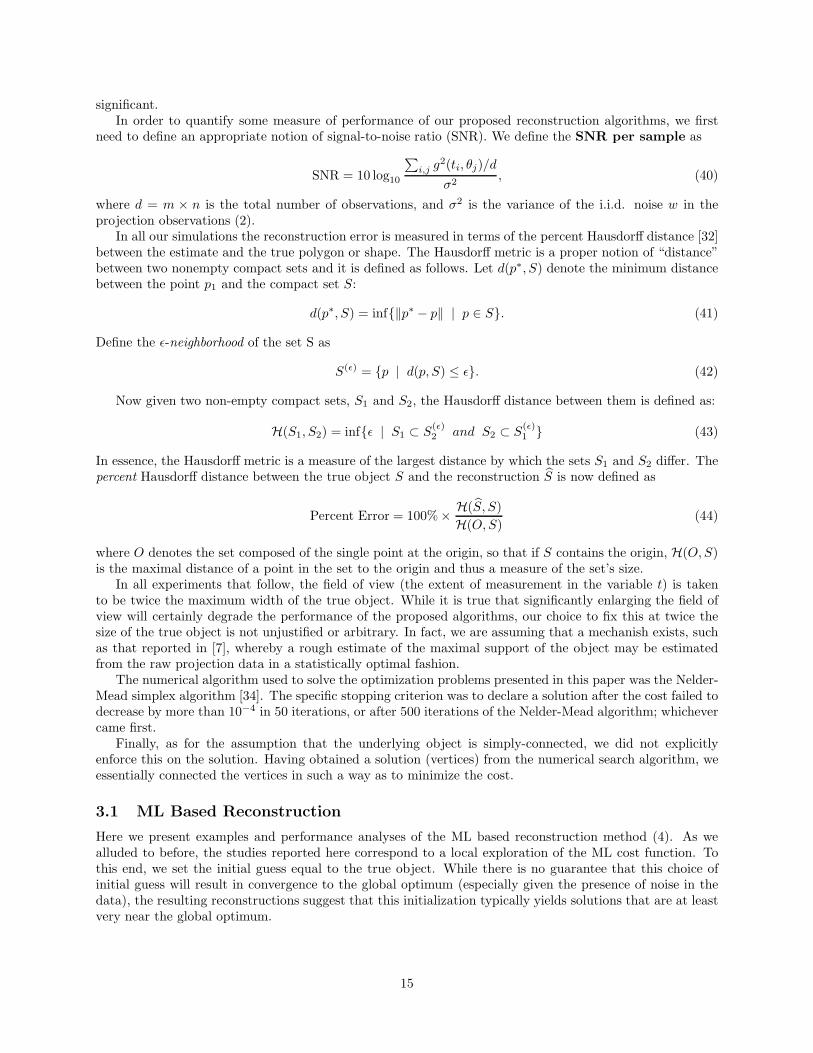
-3 -2 -1 0 1 2 3-3

-2

-1

0

1

2

3

Figure 5: Hexagon example. SNR= 0 dB 50 views, 20 samples/view: True(-), Reconstruction(- -).%Error=9.6

3.1.2 Effect of Noise on Performance

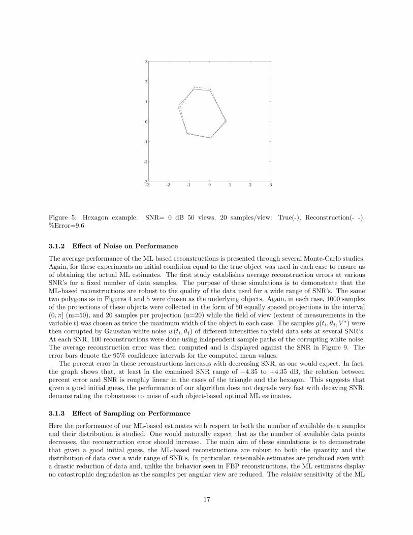
The average performance of the ML based reconstructions is presented through several Monte-Carlo studies.Again, for these experiments an initial condition equal to the true object was used in each case to ensure usof obtaining the actual ML estimates. The first study establishes average reconstruction errors at variousSNR’s for a fixed number of data samples. The purpose of these simulations is to demonstrate that theML-based reconstructions are robust to the quality of the data used for a wide range of SNR’s. The sametwo polygons as in Figures 4 and 5 were chosen as the underlying objects. Again, in each case, 1000 samplesof the projections of these objects were collected in the form of 50 equally spaced projections in the interval(0, π] (m=50), and 20 samples per projection (n=20) while the field of view (extent of measurements in thevariable t) was chosen as twice the maximum width of the object in each case. The samples g(ti, θj , V ∗) werethen corrupted by Gaussian white noise w(ti, θj) of different intensities to yield data sets at several SNR’s.At each SNR, 100 reconstructions were done using independent sample paths of the corrupting white noise.The average reconstruction error was then computed and is displayed against the SNR in Figure 9. Theerror bars denote the 95% confidence intervals for the computed mean values.

The percent error in these reconstructions increases with decreasing SNR, as one would expect. In fact,the graph shows that, at least in the examined SNR range of −4.35 to +4.35 dB, the relation betweenpercent error and SNR is roughly linear in the cases of the triangle and the hexagon. This suggests thatgiven a good initial guess, the performance of our algorithm does not degrade very fast with decaying SNR,demonstrating the robustness to noise of such object-based optimal ML estimates.

3.1.3 Effect of Sampling on Performance

Here the performance of our ML-based estimates with respect to both the number of available data samplesand their distribution is studied. One would naturally expect that as the number of available data pointsdecreases, the reconstruction error should increase. The main aim of these simulations is to demonstratethat given a good initial guess, the ML-based reconstructions are robust to both the quantity and thedistribution of data over a wide range of SNR’s. In particular, reasonable estimates are produced even witha drastic reduction of data and, unlike the behavior seen in FBP reconstructions, the ML estimates displayno catastrophic degradation as the samples per angular view are reduced. The relative sensitivity of the ML

17

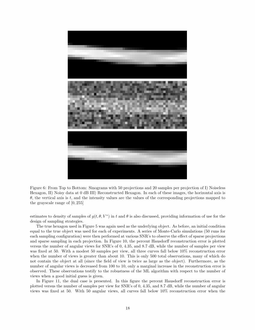
Figure 6: From Top to Bottom: Sinograms with 50 projections and 20 samples per projection of I) NoiselessHexagon, II) Noisy data at 0 dB III) Reconstructed Hexagon. In each of these images, the horizontal axis isθ, the vertical axis is t, and the intensity values are the values of the corresponding projections mapped tothe grayscale range of [0, 255]

estimates to density of samples of g(t, θ, V ∗) in t and θ is also discussed, providing information of use for thedesign of sampling strategies.

The true hexagon used in Figure 5 was again used as the underlying object. As before, an initial conditionequal to the true object was used for each of experiments. A series of Monte-Carlo simulations (50 runs foreach sampling configuration) were then performed at various SNR’s to observe the effect of sparse projectionsand sparse sampling in each projection. In Figure 10, the percent Hausdorff reconstruction error is plottedversus the number of angular views for SNR’s of 0, 4.35, and 8.7 dB, while the number of samples per viewwas fixed at 50. With a modest 50 samples per view, all three curves fall below 10% reconstruction errorwhen the number of views is greater than about 10. This is only 500 total observations, many of which donot contain the object at all (since the field of view is twice as large as the object). Furthermore, as thenumber of angular views is decreased from 100 to 10, only a marginal increase in the reconstruction error isobserved. These observations testify to the robustness of the ML algorithm with respect to the number ofviews when a good initial guess is given.

In Figure 11, the dual case is presented. In this figure the percent Hausdorff reconstruction error isplotted versus the number of samples per view for SNR’s of 0, 4.35, and 8.7 dB, while the number of angularviews was fixed at 50. With 50 angular views, all curves fall below 10% reconstruction error when the

18

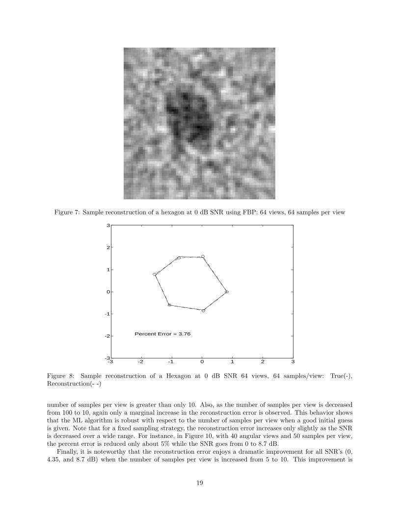
Figure 7: Sample reconstruction of a hexagon at 0 dB SNR using FBP: 64 views, 64 samples per view

-3 -2 -1 0 1 2 3-3

-2

-1

0

1

2

3

Percent Error = 3.76

Figure 8: Sample reconstruction of a Hexagon at 0 dB SNR 64 views, 64 samples/view: True(-),Reconstruction(- -)

number of samples per view is greater than only 10. Also, as the number of samples per view is decreasedfrom 100 to 10, again only a marginal increase in the reconstruction error is observed. This behavior showsthat the ML algorithm is robust with respect to the number of samples per view when a good initial guessis given. Note that for a fixed sampling strategy, the reconstruction error increases only slightly as the SNRis decreased over a wide range. For instance, in Figure 10, with 40 angular views and 50 samples per view,the percent error is reduced only about 5% while the SNR goes from 0 to 8.7 dB.

Finally, it is noteworthy that the reconstruction error enjoys a dramatic improvement for all SNR’s (0,4.35, and 8.7 dB) when the number of samples per view is increased from 5 to 10. This improvement is

19

-4 -2 0 2 40

5

10

15

20

25

SNR (dB) per sample

Per

cent

Hau

sdor

ff E

rror

Hexagon

Triangle

Figure 9: Mean performance curves for ML reconstructions of a triangle and a hexagon

0 20 40 60 80 100 1200

5

10

15

20

25

Number of Views

Perc

ent E

rror

SNR=8.7 dB

SNR=4.35 dB

SNR=0 dB

50 Samples/View

Figure 10: Performance as a function of Number of Views

more significant than that observed in Figure 10 when the number of views is increased from 5 to 10. Thisbehavior indicates that in a scenario where only a small (fixed) number of sample points can be collected, itis more beneficial to have more samples per view rather than more views.

3.2 MDL Reconstructions

Here we will examine reconstruction under the MDL criterion of (7) where we now assume that the numberof sides of the reconstructed polygon is unknown. In particular, the reconstruction experiments for the

20

0 20 40 60 80 100 1200

5

10

15

20

25

Number of Samples/View

Perc

ent E

rror

SNR=0 dB

SNR=4.35 dB

SNR=8.7 dB

50 Views

Figure 11: Performance as a Function of Number of Samples per View

hexagon in Figure 5 were repeated at SNR=0 dB assuming no knowledge of the number of sides. The MDLcriterion was employed to estimate the optimal number of sides. As in the ML algorithm, it is important tofind a good initial guess for the MDL algorithm as well. The problem is twofold. First, a reasonable guessmust be made as to the appropriate range of the number of sides. We picked a fairly small range for thenumber of sides of the reconstruction; typically, 3 to 10 sides. Next, for each number of sides, the InitialGuess algorithm was used to produce an initial guess to the optimization routine. The method for selectingthe range of the number of sides is ad hoc, but was shown to be reliable in the sense that for our simulations,the MDL cost never showed local or global minima for convex objects with number of sides larger than 10.Figure 12 shows a plot of the MDL cost corresponding to the expression in (7) versus the number of sidesfor a sample reconstruction of the hexagon in Figure 5. It can be seen that the minimum occurs at N = 6,demonstrating that the optimal MDL reconstruction will consist of 6-sides. Indeed this number coincideswith the true number of sides of the underlying object. The optimal MDL estimate is thus exactly theoptimal ML estimate for this data set presented before.

3.3 Polygonal Reconstruction of Non-polygonal Objects

In this section we wish to study the robustness of MDL-based estimates when the underlying, true object isnon-polygonal. First we examine the case of an elliptical object. We use the MDL formulation presented inthe previous section and study the behavior of the optimal reconstructions at two different SNR’s. To thisend, let the true object (that which generated the data) be a binary ellipse whose boundary is given by:{

x, y | (x− 12

)2 +(y + 1

2 )2

9/4= 1}. (45)

The above relation defines an ellipse centered at the point (1/2,−1/2) whose major and minor axes arealigned with the coordinate axes with lengths 1 and 3/2, respectively.

One thousand (1000) noisy samples of the Radon transform of this ellipse were generated (m=50 equallyspaced angular views in (0,π], and n=20 samples per view) at SNR’s of 0 and 2.17 dB respectively for 50different sample paths of the corrupting noise. For each set of data, reconstructions were performed usingthe ML algorithm with 3, 4, 5, 6, 7, and 8 sides together with the initial guess algorithm. The MDL cost in(7) was then computed for each of these reconstructions. The ensemble mean of this cost over the 50 runs,

21

3.5 4 4.5 5 5.5 6 6.5 7 7.5 8 8.51190

1195

1200

1205

1210

1215

1220

1225

Number of sides (N)

Min

imum

MD

L c

ost

Figure 12: Cost vs number of sides for the hexagon in Figure 5

2 4 6 8 101050

1100

1150

1200

Number of sides (N)

MD

L c

ost

2 4 6 8 101050

1100

1150

1200

Number of sides (N)

MD

L c

ost

SNR=0 dBSNR=2.17 dB

0

0

5-sided reconstruction, SNR=2.17 dB 6-sided reconstruction, SNR=0 dB

0

Figure 13: Minimum MDL costs and Sample Reconstructions for an Ellipse

for each value of N , is presented in the top part of Figure 13. The error bars denote the 95% confidenceintervals for the computed mean values. The top left curve corresponding to the SNR= 2.17 dB case displaysits minimum at N = 5. This behavior indicates that the average optimal MDL reconstruction uses 5 sides atthis noise level. A corresponding typical such five-sided reconstruction of the ellipse is displayed on the lowerleft plot of Figure 13 together with the true ellipse. The upper right curve corresponding to the SNR= 0 dBcase displays its minimum at N = 6 which indicates that the average optimal MDL reconstruction for thiscase uses 6 sides. The MDL cost curve for this lower SNR case has now become quite flat however, showingthat the reconstruction with N from 4 to 6 are all about equally explanatory of the data. Although the curves

22

-2 0 2-3

-2

-1

0

1

2

9-sided

-2 0 2-3

-2

-1

0

1

2

8-sided

-2 0 2-3

-2

-1

0

1

2

7-sided

-2 0 2-3

-2

-1

0

1

2

6-sided

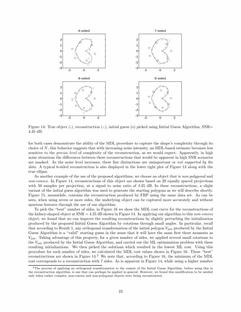
Figure 14: True object (-), reconstruction (-.), initial guess (o) picked using Initial Guess Algorithm, SNR=4.35 dB.

for both cases demonstrate the ability of the MDL procedure to capture the shape’s complexity through itschoice of N , this behavior suggests that with increasing noise intensity, an MDL-based estimate becomes lesssensitive to the precise level of complexity of the reconstruction, as we would expect. Apparently, in highnoise situations the differences between these reconstructions that would be apparent in high SNR scenariosare masked. As the noise level increases, these fine distinctions are unimportant or not supported by thedata. A typical 6-sided reconstruction is also displayed in the lower right plot of Figure 13 along with thetrue ellipse.

As another example of the use of the proposed algorithms, we choose an object that is non-polygonal andnon-convex. In Figure 14, reconstructions of this object are shown based on 20 equally spaced projectionswith 50 samples per projection, at a signal to noise ratio of 4.35 dB. In these reconstructions, a slightvariant of the initial guess algorithm was used to generate the starting polygons as we will describe shortly.Figure 15, meanwhile, contains the reconstruction produced by FBP using the same data set. As can beseen, when using seven or more sides, the underlying object can be captured more accurately and withoutspurious features through the use of our algorithm.

To pick the “best” number of sides, in Figure 16 we show the MDL cost curve for the reconstructions ofthe kidney-shaped object at SNR = 4.35 dB shown in Figure 14. In applying our algorithm to this non-convexobject, we found that we can improve the resulting reconstructions by slightly perturbing the initializationproduced by the proposed Initial Guess Algorithm by rotations through small angles. In particular, recallthat according to Result 1, any orthogonal transformation of the initial polygon Vinit produced by the InitialGuess Algorithm is a “valid” starting guess in the sense that it will have the same first three moments asVinit. Taking advantage of this property, for a given number of sides, we applied several small rotations tothe Vinit produced by the Initial Guess Algorithm, and carried out the ML optimization problem with theseresulting initializations. We then picked the solutions which resulted in the lowest ML cost. Using thisprocedure for each number of sides, we calculated the MDL cost values shown in Figure 16. These “best”reconstructions are shown in Figure 14.2 We note that, according to Figure 16, the minimum of the MDLcost corresponds to a reconstruction with 7 sides. As is apparent in Figure 14, while using a higher number

2The process of applying an orthogonal transformation to the output of the Initial Guess Algorithm, before using this inthe reconstruction algorithm, is one that can perhaps be applied in general. However, we found this modification to be neededonly when rather complex, non-convex and non-polygonal objects were being reconstructed.

23

Figure 15: FBP Reconstruction of non-polygonal, non-convex Object: 3rd order Butterworth filter with 0.15normalized cutoff frequency, SNR=4.35 dB

5 6 7 8 9 10 111110

1120

1130

1140

1150

1160

1170

1180

Number of sides

MD

L co

st

Figure 16: MDL cost curve for the reconstruction of the kidney-shaped object with the Initial Guess Algo-rithm used.

of vertices beyond 7 does improve the reconstructions somewhat, it does not yield significantly better results.This fact is directly reflected in the MDL cost curve becoming increasingly flat beyond 7 sides.

24

0 20 40 60 80 1000

50

100

150

200

250

300

350

Realizations Number

Per

cent

Hau

sdor

ff E

rror

Outlier --->

Outlier --->

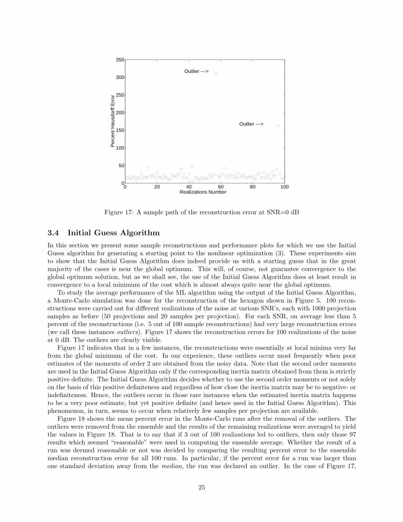
Figure 17: A sample path of the reconstruction error at SNR=0 dB

3.4 Initial Guess Algorithm

In this section we present some sample reconstructions and performance plots for which we use the InitialGuess algorithm for generating a starting point to the nonlinear optimization (3). These experiments aimto show that the Initial Guess Algorithm does indeed provide us with a starting guess that in the greatmajority of the cases is near the global optimum. This will, of course, not guarantee convergence to theglobal optimum solution, but as we shall see, the use of the Initial Guess Algorithm does at least result inconvergence to a local minimum of the cost which is almost always quite near the global optimum.

To study the average performance of the ML algorithm using the output of the Initial Guess Algorithm,a Monte-Carlo simulation was done for the reconstruction of the hexagon shown in Figure 5. 100 recon-structions were carried out for different realizations of the noise at various SNR’s, each with 1000 projectionsamples as before (50 projections and 20 samples per projection). For each SNR, on average less than 5percent of the reconstructions (i.e. 5 out of 100 sample reconstructions) had very large reconstruction errors(we call these instances outliers). Figure 17 shows the reconstruction errors for 100 realizations of the noiseat 0 dB. The outliers are clearly visible.

Figure 17 indicates that in a few instances, the reconstructions were essentially at local minima very farfrom the global minimum of the cost. In our experience, these outliers occur most frequently when poorestimates of the moments of order 2 are obtained from the noisy data. Note that the second order momentsare used in the Initial Guess Algorithm only if the corresponding inertia matrix obtained from them is strictlypositive definite. The Initial Guess Algorithm decides whether to use the second order moments or not solelyon the basis of this positive definiteness and regardless of how close the inertia matrix may be to negative- orindefiniteness. Hence, the outliers occur in those rare instances when the estimated inertia matrix happensto be a very poor estimate, but yet positive definite (and hence used in the Initial Guess Algorithm). Thisphenomenon, in turn, seems to occur when relatively few samples per projection are available.

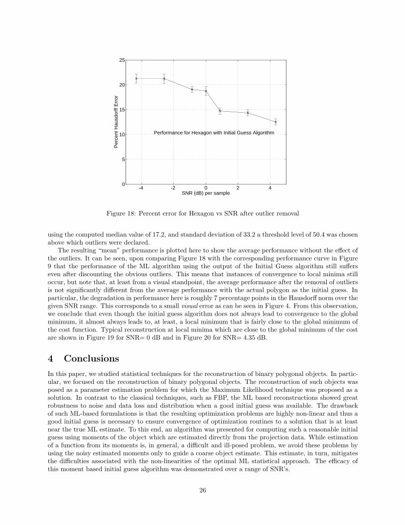
Figure 18 shows the mean percent error in the Monte-Carlo runs after the removal of the outliers. Theoutliers were removed from the ensemble and the results of the remaining realizations were averaged to yieldthe values in Figure 18. That is to say that if 3 out of 100 realizations led to outliers, then only those 97results which seemed “reasonable” were used in computing the ensemble average. Whether the result of arun was deemed reasonable or not was decided by comparing the resulting percent error to the ensemblemedian reconstruction error for all 100 runs. In particular, if the percent error for a run was larger thanone standard deviation away from the median, the run was declared an outlier. In the case of Figure 17,

25

-4 -2 0 2 40

5

10

15

20

25

SNR (dB) per sample

Per

cent

Hau

sdor

ff E

rror

Performance for Hexagon with Initial Guess Algorithm

Figure 18: Percent error for Hexagon vs SNR after outlier removal

using the computed median value of 17.2, and standard deviation of 33.2 a threshold level of 50.4 was chosenabove which outliers were declared.

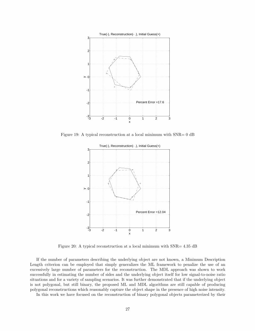
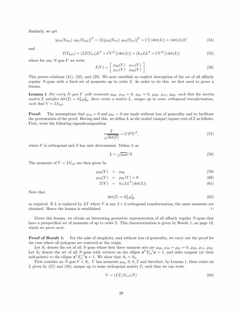
The resulting “mean” performance is plotted here to show the average performance without the effect ofthe outliers. It can be seen, upon comparing Figure 18 with the corresponding performance curve in Figure9 that the performance of the ML algorithm using the output of the Initial Guess algorithm still sufferseven after discounting the obvious outliers. This means that instances of convergence to local minima stilloccur, but note that, at least from a visual standpoint, the average performance after the removal of outliersis not significantly different from the average performance with the actual polygon as the initial guess. Inparticular, the degradation in performance here is roughly 7 percentage points in the Hausdorff norm over thegiven SNR range. This corresponds to a small visual error as can be seen in Figure 4. From this observation,we conclude that even though the initial guess algorithm does not always lead to convergence to the globalminimum, it almost always leads to, at least, a local minimum that is fairly close to the global minimum ofthe cost function. Typical reconstruction at local minima which are close to the global minimum of the costare shown in Figure 19 for SNR= 0 dB and in Figure 20 for SNR= 4.35 dB.

4 Conclusions

In this paper, we studied statistical techniques for the reconstruction of binary polygonal objects. In partic-ular, we focused on the reconstruction of binary polygonal objects. The reconstruction of such objects wasposed as a parameter estimation problem for which the Maximum Likelihood technique was proposed as asolution. In contrast to the classical techniques, such as FBP, the ML based reconstructions showed greatrobustness to noise and data loss and distribution when a good initial guess was available. The drawbackof such ML-based formulations is that the resulting optimization problems are highly non-linear and thus agood initial guess is necessary to ensure convergence of optimization routines to a solution that is at leastnear the true ML estimate. To this end, an algorithm was presented for computing such a reasonable initialguess using moments of the object which are estimated directly from the projection data. While estimationof a function from its moments is, in general, a difficult and ill-posed problem, we avoid these problems byusing the noisy estimated moments only to guide a coarse object estimate. This estimate, in turn, mitigatesthe difficulties associated with the non-linearities of the optimal ML statistical approach. The efficacy ofthis moment based initial guess algorithm was demonstrated over a range of SNR’s.

26

-3 -2 -1 0 1 2 3-3

-2

-1

0

1

2

3

x

y

True(-), Reconstruction(- .), Initial Guess(+)

Percent Error =17.6

Figure 19: A typical reconstruction at a local minimum with SNR= 0 dB

-3 -2 -1 0 1 2 3-3

-2

-1

0

1

2

3

x

y

True(-), Reconstruction(- .), Initial Guess(+)

Percent Error =12.04

Figure 20: A typical reconstruction at a local minimum with SNR= 4.35 dB

If the number of parameters describing the underlying object are not known, a Minimum DescriptionLength criterion can be employed that simply generalizes the ML framework to penalize the use of anexcessively large number of parameters for the reconstruction. The MDL approach was shown to worksuccessfully in estimating the number of sides and the underlying object itself for low signal-to-noise ratiosituations and for a variety of sampling scenarios. It was further demonstrated that if the underlying objectis not polygonal, but still binary, the proposed ML and MDL algorithms are still capable of producingpolygonal reconstructions which reasonably capture the object shape in the presence of high noise intensity.

In this work we have focused on the reconstruction of binary polygonal objects parameterized by their

27

vertices. The ML and MDL-based techniques used here may also be applied to more general object pa-rameterizations. In particular, while we used the (estimated) moments of the object only as the basis forgenerating an initial guess, it is, in some cases, possible to actually parameterize the object entirely throughits moments. For instance, Davis [35] has shown that a triangle in the plane is uniquely determined by itsmoments up to order 3, while in [27, 33] we have generalized this result to show that the vertices of anysimply connected nondegenerate N -gon are uniquely determined by its moments up to order 2N − 3.

More generally, a square integrable function defined over a compact region of the plane is completelydetermined by the entire set of its moments [31, 29, 28]. In reality we will only have access to a finiteset of these moments and these numbers, coming from estimates, will themselves be inexact and noisy.While estimation of the moments of a function based on its projections is a convenient linear problem,inversion of the resulting finite set of moments to obtain the underlying function estimate is a difficultand ill-posed problem. These observations suggest a spectrum of ways in which to use moments in ourreconstruction problems. At one extreme, only a few moments are used in a sub-optimal way to generatea simple initialization for solution of a hard, non-linear estimation problem. At the other extreme, themoments are themselves used in an optimal reconstruction scheme. In [27, 26] we have studied regularizedvariational formulations for the reconstruction of a square integrable function from noisy estimates of a finitenumber of its moments. We have also studied [33] array-processing-based algorithms for the reconstructionof binary polygonal objects from a finite number of their moments.

5 Acknowledgements

The authors wish to acknowledge the anonymous reviewers for their extremely constructive and usefulsuggestions.

A Theoretical Results on the Initial Guess Algorithm

In this section we present some theoretical justification for the initial guess algorithm. To start, we statesome elementary properties of unit area polygons Vref(N) whose vertices are the scaled N th roots of unity(in counter-clockwise direction) as defined by (18). From [27], it is a matter of some algebraic manipulationsto show that the regular polygon Vref(N) has moments of up to order 2 given by

µ00(Vref(N)) = 1 (46)µ10(Vref(N)) = µ01(Vref(N)) = 0 (47)

µ20(Vref(N)) = µ02(Vref(N)) =1

4N tan( πN )= kN (48)

µ11(Vref(N)) = 0 (49)

Now let Vinit be an affine transformation of Vref as

Vinit = LVref(N) + [C | C| · · · |C] (50)

for some linear transformation L and some 2× 1 vector C. Let O(Vinit) denote the closed, binary polygonalregion enclosed by the N -gon Vinit. Now by considering the change of variables z = Lu, and dropping theexplicit dependences on N we have

µ00(Vinit) =∫ ∫O(Vinit)

dz, (51)

=∫ ∫O(Vref)

|det(L)|du, (52)

= µ00(Vref)|det(L)| = |det(L)| (53)

28

Similarly, we get

[µ10(Vinit) µ01(Vinit)]T =(L[µ10(Vref) µ01(Vref)]T + C

)|det(L)| = |det(L)|C (54)

andI(Vinit) = (LI(Vref)LT + CCT )|det(L)| = (kNLLT + CCT )|det(L)| (55)

where for any N -gon V we write

I(V ) =[µ20(V ) µ11(V )µ11(V ) µ02(V )

]. (56)

This proves relations (21), (22), and (23). We next establish an explicit description of the set of all affinelyregular N -gons with a fixed set of moments up to order 2. In order to do this, we first need to prove alemma.

Lemma 1 For every N -gon V with moments µ00, µ10 = 0, µ01 = 0, µ20, µ11, µ02, such that the inertiamatrix I satisfies det(I) = k2

Nµ400, there exists a matrix L, unique up to some orthogonal transformation,

such that V = LVref .

Proof: The assumptions that µ10 = 0 and µ01 = 0 are made without loss of generality and to facilitatethe presentation of the proof. Having said this, we define L as the scaled (unique) square root of I as follows.First, write the following eigendecomposition

I√det(I)

= US2UT , (57)

where U is orthogonal and S has unit determinant. Define L as

L =√µ00US. (58)

The moments of V = LVref are then given by

µ00(V ) = µ00 (59)µ10(V ) = µ01(V ) = 0 (60)I(V ) = kNLL

T |det(L)| (61)

Note thatdet(I) = k2

Nµ400 (62)

as required. If L is replaced by LT where T is any 2× 2 orthogonal transformation, the same moments areobtained. Hence the lemma is established. 2

Given this lemma, we obtain an interesting geometric representation of all affinely regular N -gons thathave a prespecified set of moments of up to order 2. This characterization is given by Result 1, on page 13,which we prove next.

Proof of Result 1: For the sake of simplicity, and without loss of generality, we carry out the proof forthe case where all polygons are centered at the origin.

Let S1 denote the set of all N -gons whose first three moment sets are µ00, µ10 = µ01 = 0, µ20, µ11, µ02.Let S2 denote the set of all N -gons with vertices on the ellipse zTE−1

O z = 1, and sides tangent (at theirmid-points) to the ellipse zTE−1

I z = 1. We show that S1 = S2.First consider an N -gon V ∈ S1. V has moments µ00, 0, 0, I and therefore, by Lemma 1, there exists an

L given by (57) and (58), unique up to some orthogonal matrix T1 such that we can write

V = (LT1)Vref(N) (63)

29

Let us denote the N -gons V and Vref(N) explicitly in terms of their columns as

V = [v1 | v2 | · · · | vN ] (64)Vref(N) = [w1 | w2 | · · · | wN ] (65)

so thatvj = LT1wj . (66)

It is easy to show from the definition of Vref(N) that

wTj wj = αN =1

N2 sin(2π/N)

, (67)

(wj+1 + wj)T (wj+1 + wj) = 4βN =

4N tan(π/N)

. (68)

Now to show that V ∈ S2, we prove that

vTj E−1O vj = 1 (69)

(vj+1 + vj)T

2E−1I

(vj+1 + vj)2

= 1 (70)

for j = 1, 2 · · · N , where by convention, N + 1 = 1. Using (57) and (58), we can write

vTj E−1O vj =

µ00kNαN

vTj I−1vj . (71)

=µ00kNαN

1kNµ2

00

µ00wTj T

T1 SU

TUS−2UTUST1wj . (72)

=1αN

wTj wj . (73)

= 1. (74)

Similarly,

(vj+1 + vj)T

2E−1I

(vj+1 + vj)2

=14µ00kNβN

1kNµ2

00

µ00(vj+1 + vj)TI−1(vj+1 + vj)

=1

4βN(wj+1 + wj)T (wj+1 + wj) (75)

= 1 (76)

Hence, V ∈ S2.Now assume that V ∈ S2. Then, by assumption,

vTj E−1O vj = 1 (77)

(vj+1 + vj)T

2E−1I

(vj+1 + vj)2

= 1 (78)

Define the vertices of the related N -gon Z as

zj =1

√αNµ00

S−1UT vj . (79)

where S and U are given by the normalized eigendecomposition of I given in (57). Writing (77) and (78) interms of zj, after some algebraic manipulations, we get

zTj zj = 1 (80)

(zj+1 + zj)T

2(zj+1 + zj)

2= cos2(

π

N) (81)

30

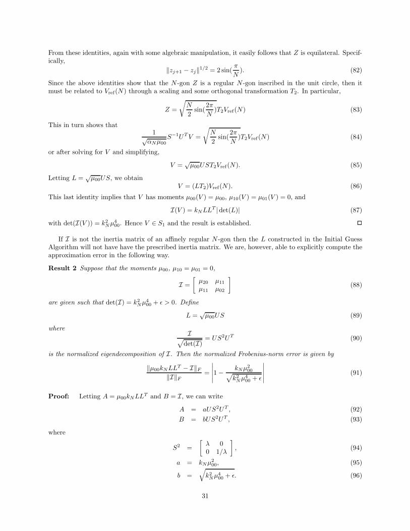
From these identities, again with some algebraic manipulation, it easily follows that Z is equilateral. Specif-ically,

‖zj+1 − zj‖1/2 = 2 sin(π

N). (82)

Since the above identities show that the N -gon Z is a regular N -gon inscribed in the unit circle, then itmust be related to Vref(N) through a scaling and some orthogonal transformation T2. In particular,

Z =

√N

2sin(

2πN

)T2Vref(N) (83)

This in turn shows that1

√αNµ00

S−1UTV =

√N

2sin(

2πN

)T2Vref(N) (84)

or after solving for V and simplifying,

V =√µ00UST2Vref(N). (85)

Letting L =√µ00US, we obtain

V = (LT2)Vref(N). (86)

This last identity implies that V has moments µ00(V ) = µ00, µ10(V ) = µ01(V ) = 0, and

I(V ) = kNLLT |det(L)| (87)

with det(I(V )) = k2Nµ

400. Hence V ∈ S1 and the result is established. 2

If I is not the inertia matrix of an affinely regular N -gon then the L constructed in the Initial GuessAlgorithm will not have have the prescribed inertia matrix. We are, however, able to explicitly compute theapproximation error in the following way.

Result 2 Suppose that the moments µ00, µ10 = µ01 = 0,

I =[µ20 µ11

µ11 µ02

](88)

are given such that det(I) = k2Nµ

400 + ε > 0. Define

L =√µ00US (89)

whereI√

det(I)= US2UT (90)

is the normalized eigendecomposition of I. Then the normalized Frobenius-norm error is given by

‖µ00kNLLT − I‖F

‖I‖F=

∣∣∣∣∣1− kNµ200√

k2Nµ

400 + ε

∣∣∣∣∣ (91)

Proof: Letting A = µ00kNLLT and B = I, we can write

A = aUS2UT , (92)B = bUS2UT , (93)

where

S2 =[λ 00 1/λ

], (94)

a = kNµ200, (95)

b =√k2Nµ

400 + ε. (96)

31

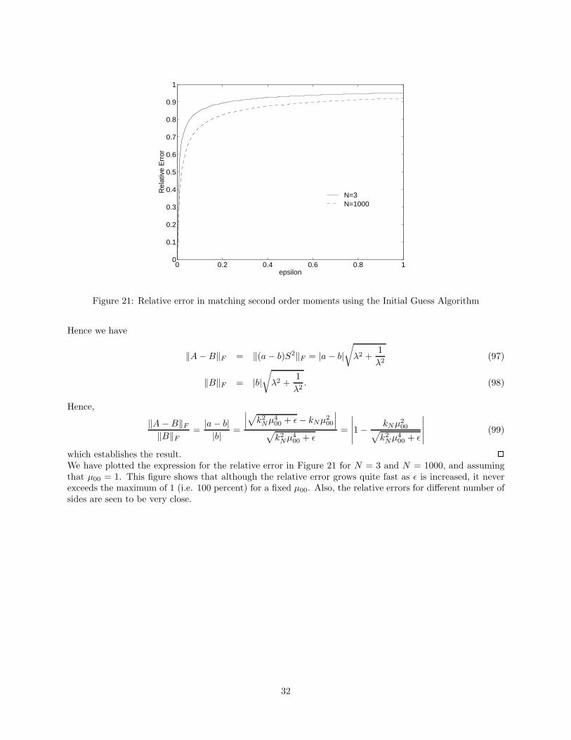
0 0.2 0.4 0.6 0.8 10

0.1

0.2

0.3

0.4

0.5

0.6

0.7

0.8

0.9

1

epsilon

Rel

ativ

e E

rror

N=3 N=1000

Figure 21: Relative error in matching second order moments using the Initial Guess Algorithm

Hence we have

‖A−B‖F = ‖(a− b)S2‖F = |a− b|√λ2 +

1λ2

(97)

‖B‖F = |b|√λ2 +

1λ2. (98)

Hence,

‖A−B‖F‖B‖F

=|a− b||b| =

∣∣∣√k2Nµ

400 + ε− kNµ2

00

∣∣∣√k2Nµ

400 + ε

=

∣∣∣∣∣1− kNµ200√

k2Nµ

400 + ε

∣∣∣∣∣ (99)

which establishes the result. 2

We have plotted the expression for the relative error in Figure 21 for N = 3 and N = 1000, and assumingthat µ00 = 1. This figure shows that although the relative error grows quite fast as ε is increased, it neverexceeds the maximum of 1 (i.e. 100 percent) for a fixed µ00. Also, the relative errors for different number ofsides are seen to be very close.

32

References

[1] M. Bergstrom, J. Litton, L. Ericksson, C. Bohm, and G. Blomqvist, “Determination of object contourfrom projections for attenuation correction in cranial positron emission tomography,” J. Comput. Assist.Tomography, vol. 6, pp. 365–372, 1982.

[2] J.-P. Thirion, “Segmentation of tomographic data without image reconstruction,” IEEE Transactionson Medical Imaging, vol. 11, pp. 102–110, March 1992.

[3] N. Srinivasa, K. Ramakrishnan, and K. Rajgopal, “Detection of edges from projections,” IEEE Trans-action on Medical Imaging, vol. 11, pp. 76–80, March 1992.

[4] W. Munk and C. Wunsch, “Ocean acoustic tomography: a scheme for larger scale monitoring,” Deep-SeaResearch, vol. 26A, pp. 123–161, 1979.

[5] G. T. Hermann, Imag Reconstruction From Projections. New York: Academic Press, 1980.

[6] D. Rossi and A. Willsky, “Reconstruction from projections based on detection and estimation of objects-parts I and II: Performance analysis and robustness analysis,” IEEE Trans. on Acoustic, Speech andSignal Proc., vol. 32, pp. 886–906, August 1984.

[7] J. L. Price and A. S. Willsky, “Estimating convex sets from noisy support line measurements,” IEEETrans. Pattern Anal. Mach. Intell., vol. 12, pp. 377–389, 1990.

[8] J. L. Prince and A. S. Willsky, “A geometric projection-space reconstruction algorithm,” Linear Algebraand Its Applications, vol. 130, pp. 151–191, 1990.

[9] J. L. Prince., Geometric Model-based Estimation from Projections. PhD thesis, MIT, Dept. of EECS,1988.

[10] A. Lele, S. Kulkarni, and A. Willsky, “Convex-polygon estimation from support-line measurements andapplications to target reconstruction from laser-radar data,” Journal of the Optical Society of America,vol. 9, pp. 1693–1714, October 1992.

[11] A. Lele, “Convex set estimation from support line measurements,” Master’s thesis, MIT, Dept. of EECS,1990.

[12] K. Hanson, “Tomographic reconstruction of axially symmetric objects from a single radiograph,” inHigh Speed Photography, (Strassbourg), 1984. Vol. 491.

[13] W. C. Karl, Reconstructing Objects from Projections. PhD thesis, MIT, Dept of EECS, 1991.

[14] Y. Bresler and A. Macovski, “Estimation of 3-d shape of blood vessels from X-ray images,” in Proc.IEEE Int. Conf. on Acoustics, Speech and Signal Processing, March 1984.

[15] Y. Bresler, J. Fessler, and A. Macovski, “A bayesian approach to reconstruction from incomplete projec-tions of a multiple object 3D domain,” IEEE Trans. on Patt. Anal. and Mach. Intel., vol. 11, pp. 840–858,August 1989.

[16] Y. Bresler and A. Macovski, “Three-dimensional reconstruction from projections with incomplete andnoisy data by object estimation,” IEEE Trans. on Acous. Speech and Signal Proc., vol. ASSP-35,pp. 1139–1152, August 1987.

[17] J. A. Fessler and A. Macovski, “Object-based 3-d reconstruction of arterial trees from magnetic reso-nance angiograms,” IEEE Trans. on Medical Imag., vol. 10, pp. 25–39, March 1991.

[18] S. Chang, “The reconstruction of binary patterns from their projections,” Comm. of the ACM, vol. 14,no. 1, 1971.

33

[19] A. Kuba, “Reconstruction of measurable plane sets from their two projections taken in arbitrary direc-tions,” Inverse Problems, vol. 7, pp. 101–107, 1991.

[20] A. Volcic, “A three point solution to Hammer’s X-ray problem,” Journal of the London MathematicalSociety, vol. 2, no. 34, pp. 349–359, 1986.

[21] P. C. Fishburn, J. Lagarias, J. Reeds, and L. A. Shepp, “Sets uniquely determined by projections onaxes I. continuous case,” SIAM J. Appl. Math., vol. 50, no. 1, pp. 288–306, 1990.

[22] R. J. Gardner, “Symmetrals and X-rays of planar convex bodies,” Arch. Math., vol. 41, pp. 183–189,1983.

[23] S. Helgason, Radon Transform. Boston: Birkhauser, 1980.

[24] H. VanTrees, Detection, Estimation, and Modulation Theory: Part I. John Wiley and Sons, 1968.

[25] J. Rissanen, Stochastic Complexity in Statistical Inquiry, vol. 15 of Series in Computer Science. WorldScientific, 1989.

[26] P. Milanfar, W. C. Karl, and A. S. Willsky, “A moment-based variational approach to tomographicreconstruction,” IEEE Transactions on Image Processing, December 1993. Submitted for Review.

[27] P. Milanfar, Geometric Estimation and Reconstruction from tomographic data. PhD thesis, MIT, De-partment of Electrical Engineering, June 1993.

[28] G. Talenti, “Recovering a function from a finite number of moments,” Inverse Problems, vol. 3, pp. 501–517, 1987.

[29] J. Shohat and J. Tamarkin, The problem of moments. New York: American Mthematical Society, 1943.

[30] M. Pawlak, “On the reconstruction aspects of moments descriptors,” IEEE Trans. Info. Theory, vol. 38,pp. 1698–1708, November 1992.

[31] N. Akhiezer, The classical moment problem and some related questions in analysis. New York: Hafner,1965.

[32] M. Berger, Geometry I and II. Springer-Verlag, 1987.

[33] P. Milanfar, G. C. Verghese, W. C. Karl, and A. S. Willsky, “Reconstructing polygons from momentswith connections to array processing,” IEEE Transactions on Signal Processing, January 1994. Sub-mitted for Review.

[34] J. Nelder and R. Mead, “A simplex method for function minimization,” Computer Journal, vol. 7,pp. 308–313, 1970.

[35] P. J. Davis, “Plane regions determined by complex moments,” Journal of Approximation Theory, vol. 19,pp. 148–153, 1977.

34

Reconstructing Binary Polygonal Objects From Projections ... · In many applications of tomography,...

Documents

Transcript of Reconstructing Binary Polygonal Objects From Projections ... · In many applications of tomography,...