12th

Numerical Towing Tank Symposium

4-6 October 2009

Cortona/Italy

Volker Bertram (Ed.)

Sponsored by

INSEAN

www.insean.it

NUMECA

www.numeca.com

CD-Adapco

www.cd-adapco.com

Germanischer Lloyd

www.gl-group.org

ONR Global

www.onrglobal.navy.mil

Dedicated to Ulderico “Paolo” Bulgarelli

for his continuous and faithful devotion to

Numerical Hydrodynamics,

both as researcher

and as inspiring guide to young researchers.

Thank you, Paolo!

This work relates to Department of the Navy Grant (Number yet unknown) issued by Office of Naval Research

Global. The United States Government has a royalty-free license throughout the world in all copyrightable

material contained herein.

Rickard Bensow

Simulating a Cavitating Propeller in a Wake Flow

Riccardo Broglia, Benjamin Bouscasse, Andrea DiMascio, Claudio Lugni

Experimental and Numerical Analysis of the Roll Decay Motion for a Patrol Boat

Jörg Brunswig, Manuel Manzke, Thomas Rung

2d RANS Simulations on Overset Grids

Danilo Calcagni, Luca Greco, Francesco Salvatore

Numerical Assessment of a BEM-based Approach for the Analysis of Ducted Propulsors

Alejandro Caldas, Adrian Sarasquete

Modification of the Rudder Geometry for Energy Efficiency Improvement on Ships

Andrea Califano

Numerical Study of a Submerged Two-Dimensional Hydrofoil using Different Solvers

Andrea Colagrossi, Salvatore Marrone, Matteo Antuono , Marshall Tulin

A Numerical Study of Breaking Bow Waves

Giuseppina Colicchio, Matteo Mattioli, Claudio Lugni, Maurizio Brocchini

Numerical Investigation of the Scouring around Pipelines

Daniele Dessi, Michele De Luca

Correlation of Bow and Stern Slamming Occurrence with Whipping Excitation for a Cruise Vessel

Andreas Feymark, Niklas Alin, Rickard Bensow, Christer Fureby

LES of the Flow around an Oscillating Cylinder

Lars Greitsch, Georg Eljardt

Simulation of Lifetime Operating Conditions as Input Parameters for CFD Calculations and Design Evalua-

tion

Jens Höpken, Bettar El Moctar, Norbert Stuntz

Simulation of a ship’s roll decay with OpenFOAM

Tobias Huuva, Magnus Pettersson

Investigating the Flexibility of Twin Screw Vessels with Various Propulsion Concepts using CFD

Alessandro Iafrati

Effects of breaking intensity on wave breaking dynamics

Sheeja Janardhanan, Krishnankutty P

Prediction of Ship Manoeuvring Hydrodynamic Coefficients Using Numerical Towing Tank Model Tests

Martin Kjellberg, Carl-Erik Janson

Numerical Optimisation of Resistance and Wake Quality for a VLCC

Marek Kraskowski

Validation of the RANSE Rigid Body Motion Computations

Alban Leroyer, Patrick Queutey, Emmanuel Guilmineau, Ganbo Deng, Michel Visonneau

New Algorithms to Speed up RANSE Computations in Hydrodynamics

Matthias Liefvendahl

Investigation of Propeller Wake Instability using LES

Nai-Xian Lu, Rickard E. Bensow

Numerical Simulations of Unsteady Cavitation Using OpenFOAM

Lars Ole Lübke

Manoeuvring Simulations of Underwater Vehicles

Michal Orych, Björn Regnström, Lars Larsson

A Surface Capturing Method in the RANS Solver SHIPFLOW

Florin Pacuraru, Adrian Lungu, Oana Marcu

Numerical Flow Simulation around an Appended Ship Hull

Eric Paterson, David Boger, Gina Casadei, Scott Miller, Hrvoje Jasak

6DOF RANS Simulations of Floating and Submerged Bodies using OpenFOAM

Alexander Phillips, Maaten Furlong, Stephen R. Turnock

Accurate capture of rudder-propeller interaction using a coupled blade element momentum-RANS approach

Auke van der Ploeg, Martin Hoekstra

Multi-Objective Optimization of a Tanker Afterbody using PARNASSOS Daniel Schmode, Volker Bertram, Matthias Tenzer

Simulating Ship Motions and Loads using OpenFOAM

Mohammad S. Seif, Abolfazl Asnaghi

Numerical Study of Cavitating Flows around a Flat Plate

Keun Woo Shin, Poul Andersen, Wen Zhong Shen

Analysis of numerical models for cavitation on 2D hydrofoil

Arthur Stück, Thomas Rung

Adjoint RANS for Hull Form Optimisation

Daniele Trimarchi, Stephen Turnock, Dominique Chapelle, Dominic J. Taunton

Fluid-Structure Interactions of Anisotropic Thin Composite Materials for Application to Sail Aerodynamics

of a Yacht in Waves

George Tzabiras, Stylianos Polyzos, G. Zarafonitis

Self-Propulsion Simulations of Passenger-Ferry Ships with Bow and Stern Propulsors

Christian Ulrich, Thomas Rung

Validation and Application of a Massively-Parallel Hydrodynamic SPH Simulation Code

Diego Villa, Stefano Brizzolara

CFD Calculations on a Cavitating Hydrofoil with OpenFOAM

Jeroen Wackers, Patrick Queutey, Michel Visonneau

Adaptive Grid Refinement for Unsteady Ship Flow and Ship Motion Simulation

Stewart Whitworth, Constantinos Zegos

Using CFD Methods to Optimise Appendage Design for Improved Propeller Inflow

Katja Wöckner

Progress in Seaway-Simulations in Compact Domains

Christian D. Wood, Dominic A. Hudson, Mingyi Tan

Numerical Simulation of Compartment Flooding for Damaged Ships

Simulating a Cavitating Propeller in Wake Flow

Rickard E Bensow Dept. of Shipping and Marine Technology

Chalmers University of Technology, Sweden, rickard.bensow@chalmers.se

A major challenge for the marine indus-try in general and for propeller designers in particular, is to reduce cavitation nui-sance. Cavitation may occur in a wide range of liquid flows and is constituted by vapor regions in the liquid, created by vaporization due to local flow induced lowering of the pressure. Experimental studies are more or less limited to visual observations and pressure pulse meas-urements, but numerical predictions are in the process of becoming a useful com-plement yielding a fairly complete pic-ture of the cavitation process. An im-proved understanding of cavitation dy-namics, using both experimental and simulation results, is a crucial component to prevent or reduce cavitation effects, such as material damage or noise, and thereby, to increase propeller perform-ance. In the present study, Large Eddy Simulation (LES) techniques are used to simulate the cavitating flow on a propel-ler, the four-bladed INSEAN E779A. Al-though an old design, the experimental database is extensive, including both PIV and LDV wake measurements [1][2][3] and cavitation observation in homogene-ous [4] and inhomogeneous [5] flow con-ditions, which makes it a good validation case. Computational studies include e.g. [6][7][8][9]. We will here simulate the cavitating case in inhomogeneous inflow conditions, thus forming a fully unsteady flow and demonstrate that the simula-tions display many of the mechanisms important to correctly predict the dy-namics of cavitation, specially the impor-tant side- and re-entrant jets typically

forming inside the initial sheet cavity in-fluencing the large scale shedding and in-teraction between the cavity and the tip vortex on the propeller. LES is based on low-pass filtering of the Navier-Stokes equations and re-tains larger flow structures and relies less on modeling compared with the averag-ing procedure in RANS, yet at a higher cost. This means that an LES solution can capture large to medium-small scale, time-dependent flow phenomena impor-tant when simulating cavitation nuisance, scales not directly available in RANS. For a stationary flow, a RANS solution is obtained several orders of magnitude faster compared with LES. If a time ac-curate solution is sought, RANS will still in general be less expensive than LES, mainly because the time step can be con-siderably longer but also due to lower requirements on the spatial resolution. When it comes to the prediction of un-steady cavitation, the necessary spatial and temporal resolution, dictated by the dynamics of the cavitating flow, is high per se, and the computational cost for RANS will approach that of LES. More-over, it is not a priori clear if the averaged flow described by the RANS equations contains the mechanisms that govern the dynamics of the cavity, while the fully unsteady flow description of-fered by LES will do so provided the mesh resolution is sufficient. The interface between liquid and vapor is captured using a Volume of Fluid (VoF) approach and a mass trans-fer model, based on the work of Kunz et al. [10], is used for the vaporization and

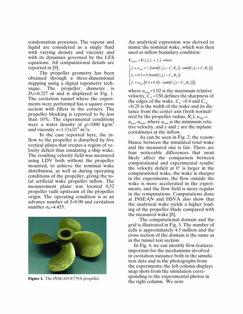
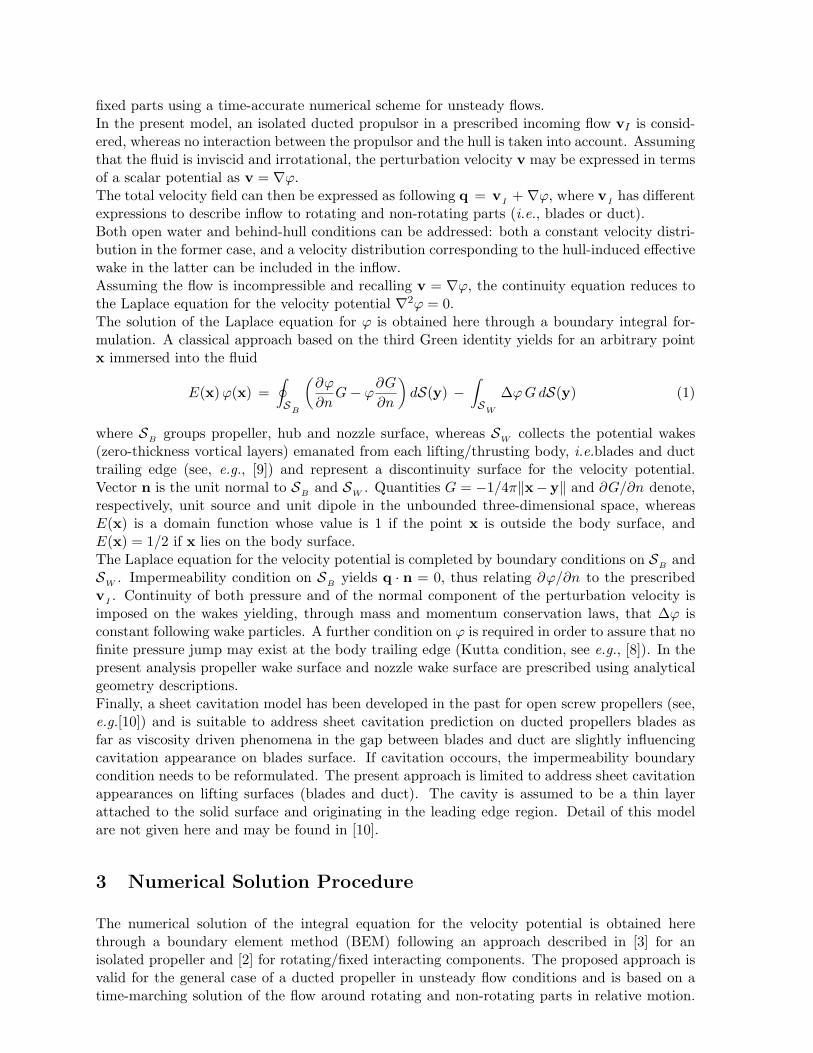
condensation processes. The vapour and liquid are considered as a single fluid with varying density and viscosity and with its dynamics governed by the LES equations. All computational details are reported in [9]. The propeller geometry has been obtained through a three-dimensional mapping using a digital topometry tech-nique. The propeller diameter is DP=0.227 m and is displayed in Fig. 1. The cavitation tunnel where the experi-ments were performed has a square cross section with fillets in the corners. The propeller blocking is reported to be less than 10%. The experimental conditions were a water density of ρ=1000 kg/m3 and viscosity ν=1.11x10-6 m2/s. In the case reported here, the in-flow to the propeller is disturbed by five vertical plates that creates a region of ve-locity deficit thus emulating a ship wake. The resulting velocity field was measured using LDV both without the propeller mounted, to achieve the nominal wake distribution, as well as during operating conditions of the propeller, giving the to-tal artificial wake propeller inflow. The measurement plane was located 0.52 propeller radii upstream of the propeller origin. The operating condition is at an advance number of J=0.90 and cavitation number σn=4.455.

Figure 1. The INSEAN E779A propeller.

An analytical expression was derived to mimic the nominal wake, which was then used as inflow boundary condition:

€

UInflow =U0 f1 f2 + f3( ), where

f1 = umax + h2 tanh CS z −CwRP( )( ) - tanh CS z + CwRP( )( )( )

f2 = 0.5 + 0.5tanh CS y −CvdRP( )( )f3 = umax 0.5 + 0.5 1- tanh CS y −CvdRP( )( )( )( )

where umax=1.02 is the maximum relative velocity, CS =150 defines the sharpness of the edges of the wake, Cw =0.4 and Cvd =0.25 is the width of the wake and its dis-tance from the center axis (both normal-ized by the propeller radius, RP), udiff = umax-umin, where umin is the minimum rela-tive velocity, and y and z are the inplane coordinates at the inflow. As can be seen in Fig. 2, the resem-blance between the simulated total wake and the measured one is fair. There are four noticeable differences that most likely affect the comparison between computational and experimental results: the velocity deficit at 0° is larger in the computational wake, the wake is sharper in the experiments, the flow outside the wake is more accelerated in the experi-ments, and the flow field is more regular in the computations. Computations done at INSEAN and HSVA also show that the analytical wake yields a higher load-ing of the propeller blade compared with the measured wake [8]. The computational domain and the grid is illustrated in Fig. 3. The number of cells is approximately 4.5 million and the cross section of the domain is the same as in the tunnel test section.

In Fig. 4, we can identify flow features important for the mechanisms involved in cavitation nuisance both in the simula-tion data and in the photographs from the experiments; the left column displays snap shots from the simulation corre-sponding to the experimental photos in the right column. We note

1. For the fully developed cavity, Fig. 4(d), the side-entrant jets along the larger part of the cavity rolling up into the tip vortex.

2. Moreover, the trailing part of the cavity is fairly distant from the blade surface, due to the internal jet, and transformed into a partly cloudy character.

3. As the blade is leaving the wake, Fig. 4(f), the cavity has more or less de-tached from the leading edge.

The simulated dynamics, shown in the left column of Fig. 4 via an isosurface of the vapor fraction α=0.5, display the same qualitative behavior as the experi-ments. However, the cavity starts to de-velop earlier and already in frame (a) a fully developed sheet cavity has devel-oped with distinct internal jets. We be-

lieve this is due to differences in the in-flow, mainly related to the lack of accel-erated flow outside the velocity deficit in the analytical inflow. In frame (e), we remark that leading edge desinence is present in the simulation, correctly re-sponding to the change in load as the blade exits the wake. In Fig. 4(g), the cavity now seems to be smaller than in the experiments but both shed cavities, one cloud shed into the tip vortex and one from the leading edge, are present and predicted at the correct location. The contradictable behavior regarding the cavity extent, i.e. that the vapor region is overpredicted in the early stages but un-derpredicted in the later stage, might partly be explained by the uncertainty in what value of vapor fraction α to com-pare.

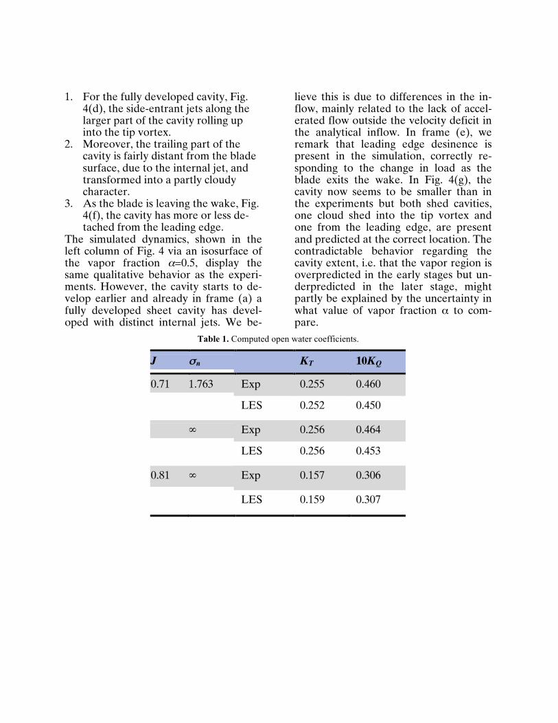
Table 1. Computed open water coefficients.

J σn KT 10KQ

0.71 1.763 Exp 0.255 0.460

LES 0.252 0.450

∞ Exp 0.256 0.464

LES 0.256 0.453

0.81 ∞ Exp 0.157 0.306

LES 0.159 0.307

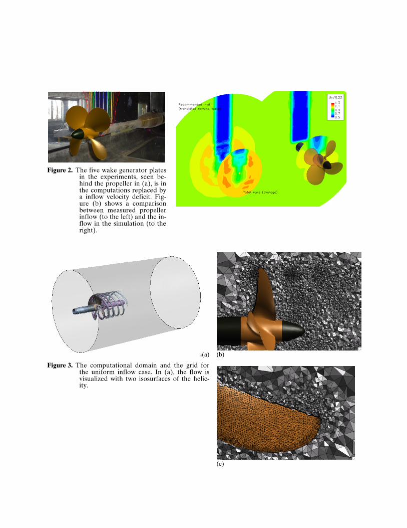
Figure 2. The five wake generator plates

in the experiments, seen be-hind the propeller in (a), is in the computations replaced by a inflow velocity deficit. Fig-ure (b) shows a comparison between measured propeller inflow (to the left) and the in-flow in the simulation (to the right).

(a)

(b) Figure 3. The computational domain and the grid for

the uniform inflow case. In (a), the flow is visualized with two isosurfaces of the helic-ity.

(c)

(a)

(b)

(c)

(d)

(e)

(f)

(g)

(h)

Figure 4. The left column shows the simulation (isosurface of vapour fraction α=0.5) and the right column the experimental photographs. The series of pictures are for propeller angles -30° (frames (a) and (b)), -10° (frames (c) and (d)), 10° (frames (e) and (f)) and 15° (frames (g) and (h)).

References [1] Stella A., Guj G., Di Felice F., “Propel-

ler wake flowfield analysis by means of LDV phase sampling technique,” Exp. in Fluids, 28, 2000.

[2] Di Florio D., Di Felice F., Romano G.P, Elefante M., “Propeller wake structure at different advance coefficients by means of PIV,” PSFVIP-3, Maui, Ha-waii, USA, 2001.

[3] Di Felice F., Felli M., Giordano G., So-ave M., “Pressure and velocity correla-tion in the wake of a propeller,” Propel-ler Shafting, Virginia Beach, Norfolk, USA, 2003.

[4] Pereira F., Salvatore F., Di Felice F., “Measurement and modeling of propel-ler cavitation in uniform inflow,” J. Fluids Engrng., 126:671–679, 2004.

[5] Pereira F., Salvatore F., Di Felice F., Soave M., “Experimental Investigation of a Cavitating Propeller in Non-Uniform Inflow,” 25th ONR Symposium on Naval Hydrodynamics, St John’s, Canada, 2004.

[6] Bensow R.E., Liefvendahl M., “Implicit and Explicit Subgrid Modeling in LES Applied to a Marine Propeller,” AIAA-2008-4144, 2008.

[7] Streckwall H., Salvatore F., “Results of the Wageningen 2007 Workshop on Propeller Open Water Calculations in-cluding Cavitation,” RINA CFD 2008, Southhampton, UK, 2008

[8] Salvatore F., Streckwall H., Terwisga T.v., “Propeller Cavitation Modelling by CFD - Results from the VIRTUE 2008 Rome Workshop,” 1st Int Sympo-sium on Marine Propulsors, Trond-heim, Norway, 2009.

[9] Bensow R.E., Huuva T., Bark G., Lie-fvendahl M., “Large Eddy Simulation of Cavitating Propeller Flows,” 27th Int. Symposium on hip Hydrodynamics, Korea, 2008.

[10] Kunz, R. F., Boger D. A., Stinebring D. R., Chyczewski T. S., Lindau J. W., Gibeling H. J., Venkateswaran S., Go-vindan T. R., “A preconditioned Na-vier-Stokes method for two-phase flows with application to cavitation predic-tion.” Computers and Fluids 29(8), 2000

Experimental and Numerical Analysis of the Roll DecayMotion for a Patrol Boat

Riccardo Broglia, Benjamin Bouscasse, Andrea Di Mascio and Claudio LugniINSEAN, Rome/Italy, c.lugni@insean.it

The analysis of the roll motion of a ship is of practical interest for both safety and comfortreasons. In this paper an experimental and numerical analysis of the roll decay for a patrol boatof the Italian Navy is carried out. Full scale trials in the Mediterranean sea in cooperation withNSWCCD (Naval Surface Warfare Center, Carderock Division) and model scale experiments atthe INSEAN towing tank have been performed. For a proper comparison, hull in fully appendedconfiguration, (i.e. with the rudders, bilge keels, fins, and propeller apparatus, including struts,A-brackets and the propeller shaft) has been considered. To properly understand the effect ofthe rotating propeller on the roll damping, model scale experiments have been performed withand without the rotating propeller. Several Froude numbers have been considered, both in fulland model scale, to highlight the effect of the ship speed on the roll damping.

Numerical simulations have been carried out for three different Froude numbers; the steadyflow around the vessel with a fixed heel angle, and the unsteady free roll decay of the vesselfrom an initial of heel angle of 10 degrees are computed. Numerical studies of the motionwith six degrees of freedom of a ship are usually performed by means of liner potential theory;therefore, viscous related phenomena are intrinsically neglected, i.e. separations and vorticalstructures are in general not taken into account or modelled by means of zero thickness vortexlayers shed from prescribed separation lines (usually coincident with geometrical singularity).Methods based on this theory give a satisfactory prediction of vertical motions, i.e. surge, heaveand pitch, and, depending on the geometry of the body, of sway and yaw motions. In any casesmall amplitude motions have to be considered. On the contrary, such techniques fail whenapplied to the analysis of the roll motion. In this case the hydrodynamics is highly non linear,because viscous effects, flow separation and vortex shedding phenomena as well as lift dampingcontribution, are important. In this case methods based on the unsteady Reynolds AveragedNavier Stokes equations (URANSE), can contribute to improve the prediction of the roll motionof a ship.

Full scale trials and model experiments An ad hoc experimental campaign for the rolldecay in calm water was performed in October 2007 on the Italian Navy ship ComandanteBettica in the Mediterranean Sea close to the coast of Sicily. The vessel, the third in theComandante class, is a patrol ship (LDWL = 80m, Bmax = 12.2m, full load displacement1520tons). The ship is equipped with two rudders, two propeller axis, bilge keels and activefins. The last ones can be activated both manually and automatically.

The trials, part of an international cooperation between NSWCCD and INSEAN, included themeasurement of the velocity field in a transversal plane of the bilge keels through the NSWCCDsubmersible PIV system, the measurement of the local hydrodynamic loads on the bilge keelthrough the use of 8 strain gages installed, and finally the measurement of the motion of theship through an inertial platform system. A wave radar system was also installed and usedto measure the wave field around the vessel. In the following we will present just the resultsrelative to the measurement of the roll motion of the ship. Major details about the PIV andlocal forces measurement can be found in [Atsavapranee et al., 2008].

The motion, in manual mode, of the active fins was used to excite the initial roll angle of theship. Once the target heel angle was reached, the motion of the fins was stopped and the roll

Figure 1: INSEAN model of the Bettica ship.

decay event of the ship occurred. The entire time history of the roll motion was acquired anda post-processing analysis was developed to window the roll decay event.

To properly get a correlation law between full scale and model scale, roll decay experimentsin calm water were performed at INSEAN. A wooden fully appended model (scale factor 20)of the ship (see fig. 1) has been used in the wave basin number 2, which is 220m long, 9mwide and 3.6m deep. This facility is characterized by a dynamometric carriage able to run ina range of velocity between 0 and 7m/s. The speed, managed via software, can be imposedwith an accuracy of 1mm/s. A suitable experimental set-up has been designed to reproducethe condition realized during the full scale trials. The model has been self propelled and leftfree to heave, pitch and roll. Because the unavailability of active fins and rudders, the hull waspartially restrained transversally. To the purpose, elastic cables hinged at the water level, havebeen used to limit the yaw, sway and surge motions of the model. During the tests the hullhas been forced to get an initial heel angle. Then by using a suitable release mechanism, themodel has been left free to damp its roll motion. Motions of the model have been measuredby using both the optical system ”Krypton” and the inertial platform ”MOTAN”. Thrust andtorque of the propellers have been also measured by using two Remmers dynamometers. Allthe signals have been acquired at a sample rate of 100Hz. Several model speeds, correspondingto Fn = 0.088, 0.106, 0.138, 0.166, 0.189, 0.227, 0.276, 0.281 and three different initial heelangles, 5, 10, 15deg respectively, have been considered.

Numerical simulations The mathematical model employed for the simulations of the flowfield is described by the Reynolds Averaged Navier–Stokes equations. The problem is closed byenforcing appropriate conditions at the physical and the computational boundaries. The numeri-cal solution of these equations is computed bu means of the solver χnavis developed at INSEAN.Details of the numerical tool can be found in [Di Mascio et al., 2008], [Di Mascio et al., 2007])[Favini et al., 1996].

The calculations were performed around a model whose scale is λ = 15. Numerical simulationswere carried out for the conditions reported in table 1. Both steady state computations and freeroll decay simulations were performed. In the steady tests, the vessel is fixed at the dynamicaltrim and sinkage provided by the experiments, and with an heel angle of ten degrees. For thefree roll decay simulations, the steady state solutions are used as initial condition, and the shipis left free to roll around her longitudinal axis after a non-dimensional time of 0.5 unit. The

Table 1: Computational parameters.Fn Rn Trim Sinkage J KT 10KQ

[deg] [mm]

0.106 4.073 106 1.24 10−2 2.175 1.0018 0.152076 0.323766

0.227 8.747 106 3.44 10−2 5.600 1.0126 0.147110 0.316111

0.337 1.300 107 4.30 10−3 14.50 1.0175 0.144845 0.312626

unsteady simulations are carried out until a negligible roll angle is reached; as expected thesteady state solution at zero heel angle is reached.

Results As an example of the numerical simulations computed, in figure 2, a sequence ofnine snapshots of the axial velocity and vorticity contours are shown for the cross sectionx = 0.111332 (around the bilge keel on the port side for the medium speed test). From thispicture, the strong interactions between the wake of the antiroll fin and the flow around thebilge keel is evident. At the first time instant, the vessel is rotating counter-clockwise (zero rollangle and maximum roll velocity). A large clockwise rotating flow (i.e. large negative values forthe axial vorticity) is generated at the tip of the bilge keel; this vortex convects high momentumfluid toward the boundary layer on the hull surface on the left of the bilge keel, and viceversalow momentum fluid from the boundary layer at the right side. As a consequence the boundarylayer on the hull surface is thinner on the left than on the right. At the same time, the wakeof the fin is on the outer face of the bilge keel and the clockwise rotating vortex shed from thetip of the antiroll fin is observable.

At the next time instant, the ship is approaching her maximum roll angle; the clockwise rotatingflow around the tip of the bilge keel weakens, while the wake of the fin is on the right face ofthe bilge keel and the tip vortex shed from the fin becomes stronger. At this time instant acounter-clockwise flow around the keel starts to appear and, at the sequent snapshot (figurenumber 2), this vortex is well developed. At the time instant 3 the tip vortex of the fin reachesits maximum strength for the medium speed case. The time shift between the evolutions of thevortices at the tip of the bilge keel and at the tip of the stabilizer is due to the distance betweenthe bilge keel and the fin, and depends on the forward speed. At this section, the maximumstrength is attained with a delay of about one fourth of the period with respect to the bilgekeel vortex at the medium speed, one eight of period at the highest speed, whereas at the lowerspeed it seems already dissipated (the figures at medium and lower speeds are not shown). Inthe following snapshots (from 4 to 6) the vessel is rolling clockwise and a counter-clockwisevortices at the tip of the fin and along the tip of the bilge keel develops. At the time instant7 the vessel is at the minimum roll angle, while in the following pictures the vessel is rotatingcounter-clockwise. A clockwise vortex along the tip of the keel develops, whereas the trace ofthe tip vortex at the fin at this section, decreases in strength at first, and then a contra-rotatingvortex starts to appear.

The time histories of the roll decay experiments, for both sea trials and model scale tests, areshown in figure 3. To understand the role of the propellers on the roll damping, experiments atthe towing tank have been performed with both self propelled condition (green line in figures 3)and towed condition (red line in the same figures).

Concerning the full scale experiments, both mean values (black line in figures) and error bars(taking into account only for the repeatability error) have been estimated. To this purpose, thenumber of the full scale trials considered to determine the standard deviation and the meanvalue is reported in the legend of each figure. Note as the error bars were not estimated atFn = 0.166 because of the low number of runs available. A first look at the full scale trial

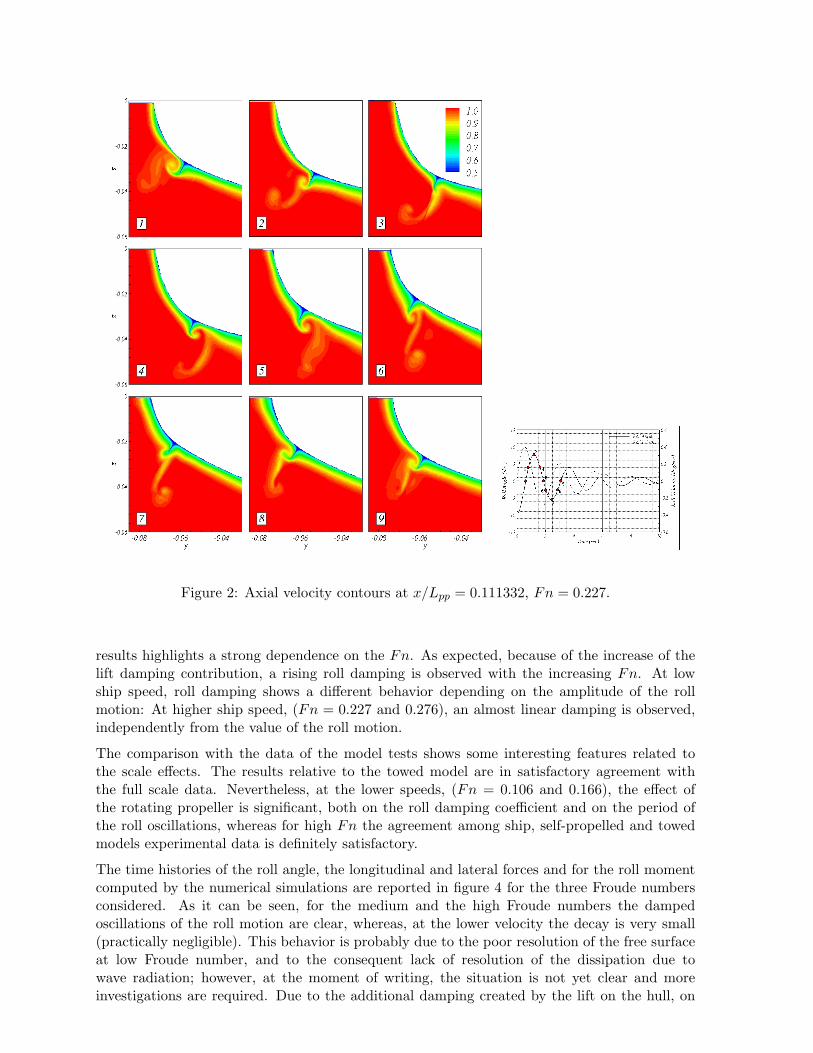
Figure 2: Axial velocity contours at x/Lpp = 0.111332, Fn = 0.227.

results highlights a strong dependence on the Fn. As expected, because of the increase of thelift damping contribution, a rising roll damping is observed with the increasing Fn. At lowship speed, roll damping shows a different behavior depending on the amplitude of the rollmotion: At higher ship speed, (Fn = 0.227 and 0.276), an almost linear damping is observed,independently from the value of the roll motion.

The comparison with the data of the model tests shows some interesting features related tothe scale effects. The results relative to the towed model are in satisfactory agreement withthe full scale data. Nevertheless, at the lower speeds, (Fn = 0.106 and 0.166), the effect ofthe rotating propeller is significant, both on the roll damping coefficient and on the period ofthe roll oscillations, whereas for high Fn the agreement among ship, self-propelled and towedmodels experimental data is definitely satisfactory.

The time histories of the roll angle, the longitudinal and lateral forces and for the roll momentcomputed by the numerical simulations are reported in figure 4 for the three Froude numbersconsidered. As it can be seen, for the medium and the high Froude numbers the dampedoscillations of the roll motion are clear, whereas, at the lower velocity the decay is very small(practically negligible). This behavior is probably due to the poor resolution of the free surfaceat low Froude number, and to the consequent lack of resolution of the dissipation due towave radiation; however, at the moment of writing, the situation is not yet clear and moreinvestigations are required. Due to the additional damping created by the lift on the hull, on

Figure 3: Roll decay experiments; time histories of the roll angle. Model scale, both in selfpropelled (green line) and tow (red line) conditions, and full scale (black line) data, are repre-sented.

the stabilizers and on the bilge keels, the damping of the roll motion increases with the speedof the vessel, whereas the period of the oscillation is almost constant.

In figure 3 numerical results (in blue) are superimposed to model and full scale trials for Fn =0.227; it can be seen that the numerical computation underestimates the damping of the rollmotion. This underestimation could be due to different reasons: first of all, the numericalpropeller model mimics only the effects of the fluid acceleration and swirl on the flow field,without providing any contribution to the roll damping due to the solid wall; the lack in thegrid resolution could be another reason: a poor grid resolution on the free-surface can induce apoor prediction of the wave radiation damping (even if it is usually small for the roll motion).Moreover, a coarse grid around the appendages causes an underestimation of damping inducedby small vortices. Turbulence modeling could be an additional source of error in the dampingestimation. Finally, the different scale factor and the different constraints used in the modeltests and numerical computation, could be a further reason for these discrepancies. However,the problem is still under analysis and any final conclusion can be drawn.

CONCLUSIONS The analysis of the roll decay motion for a patrol boat of the Italian Navyhas been carried out by means of sea trials, model scale experiments and numerical simulations.The effect of the rotating propeller has been considered in the model experiments. A quiteevident contribution was shown at the low Fn. Better agreement between model and full scaledata was observed by increasing the Fn. Numerical simulations have been used for the analysisof the local flow field around the vessel; the snapshots of the axial velocity on a cross sectionbetween the stabilizer fin and the bilge keel highlights the formation of longitudinal vortex along

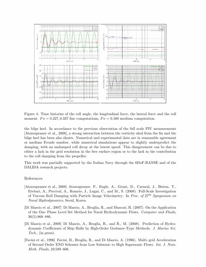
Figure 4: Time histories of the roll angle, the longitudinal force, the lateral force and the rollmoment. Fn = 0.227, 0.337 fine computations, Fn = 0.160 medium computation.

the bilge keel. In accordance to the previous observation of the full scale PIV measurements[Atsavapranee et al., 2008], a strong interaction between the vorticity shed from the fin and thebilge keel has been also shown. Numerical and experimental data are in reasonable agreementat medium Froude number, while numerical simulations appear to slightly underpredict thedamping, with an undamped roll decay at the lowest speed. This disagreement can be due toeither a lack in the grid resolution in the free surface region or to the lack in the contributionto the roll damping from the propeller.

This work was partially supported by the Italian Navy through the 6DoF-RANSE and of theDALIDA research projects.

References

[Atsavapranee et al., 2008] Atsavapranee, P., Engle, A., Grant, D., Carneal, J., Beirne, T.,Etebari, A., Percival, A., Rosario, J., Lugni, C., and M., S. (2008). Full-Scale Investigationof Viscous Roll Damping with Particle Image Velocimetry. In Proc. of 27th Symposium onNaval Hydrodynamics, Seoul, Korea.

[Di Mascio et al., 2007] Di Mascio, A., Broglia, R., and Muscari, R. (2007). On the Applicationof the One–Phase Level Set Method for Naval Hydrodynamic Flows. Computer and Fluids,36(5):868–886.

[Di Mascio et al., 2008] Di Mascio, A., Broglia, R., and R., M. (2008). Prediction of Hydro-dynamic Coefficients of Ship Hulls by High-Order Godunov-Type Methods. J. Marine Sci.Tech., (in press).

[Favini et al., 1996] Favini, B., Broglia, R., and Di Mascio, A. (1996). Multi–grid Accelerationof Second Order ENO Schemes from Low Subsonic to High Supersonic Flows. Int. J. Num.Meth. Fluids, 23:589–606.

2D RANS Simulations on Overset Grids

Jorg Brunswig, Manuel Manzke and Thomas Rung

joerg.brunswig@tu-harburg.de

Hamburg University of Technology (TUHH), Germany

Institute of Fluid Dynamics and Ship Theory (M-8)

Rigid computational grids represent a strong limi-tation on the geometric complexity of CFD compu-tations, particularly when components of the tech-nical structure to be modelled move relatively toeach other. Several techniques have been devel-oped in the past to overcome these problems. Usinga sliding interface, simple types of motion can bemodelled. Special care with respect to mesh gen-eration has to be taken, though. For pure rota-tions around a given axis for example, the interfacebetween the grid parts must be perfectly cylindri-cal and the cell sizes on each side of the interfaceshould be equal. Another method is mesh distor-tion. Arbitrary motions with relatively small am-plitudes can be modelled, larger amplitudes oftenlead to highly distorted cells which can make anaccurate solution of the problem impossible. Effi-cient regridding algorithms are almost impossibleto realize for hex meshes and complex geometries.The method is computationally quite expensive,but very flexible with respect to types of motion.Overlapping grids (often called overset / chimeragrids) are a very versatile method regarding com-plex moving geometries. Very close arrangements ofmoving parts and intersecting motion paths are pos-sible to model. The method can strongly facilitatethe grid generation process and improve the qualityof the meshes. This technique is rather complex toimplement, though, especially for parallel computa-tions. Nevertheless, the overlapping grids techniqueseemed to represent the best tradeoff between flexi-bility and feasibility (in terms of programming andcomputational effort), so it was decided to be im-plemented in our simulation tool FreSCo+.

FreSCo+

FreSCo+ is a spin-off of FreSCo, a joint de-velopment of Hamburg University of Technology(TUHH), Hamburgische Schiffbau-Versuchsanstalt(HSVA) and Maritime Research Institute Nether-lands (MARIN). The original code was developedwithin the scope of the EU initiative VIRTUE.The procedure uses a segregated algorithm basedon the strong conservation form of the momen-tum equations. It employs a cell-centered, co-located storage arrangement for all transport prop-

erties. Structured and unstructured grids, basedon arbitrary polyhedral cells or hanging nodes, canbe used. The implicit numerical approximationis second-order accurate in space and time. In-tegrals are approximated using the conventionalmid-point rule. The solution is iterated to conver-gence using a pressure-correction scheme. Variousturbulence-closure models are available with respectto statistical (RANS) or scale-resolving (LES, DES)approaches. Two-phase flows are addressed byinterface-capturing methods based upon the Level-Set or Volume-of-Fluid (VOF) technique. Since thedata structure is generally unstructured, suitablepre-conditioned iterative sparse-matrix solvers forsymmetric and non-symmetric systems (e.g. GM-RES, BiCG, QMR, CGS or BiCGStab) can beemployed. The algorithm is parallelised using adomain-decomposition technique based on a SingleProgram Multiple Data (SPMD) message-passingmodel, i.e. each process runs the same program onits own subset of data. Inter-processor communi-cation employs the MPI communications protocol.Load balancing is achieved using the ParMETISpartitioning software.

Overlapping Grids

The overlapping grids technique implemented inFreSCo+ refers to the mass-conservative approachdescribed by [1]. The grid coupling is realized byinterpolating field values φ from a cell center on adonor grid to a cell center on a target grid:

φtarget = aiφdonori + ajφ

donorj + akφ

donork (1)

The indices i,j,k form the interpolation stencil, ai,aj and ak are the associated interpolation weights.Because the equations of all grids are assembledinto one equation system, the grid coupling can beformulated implicitly (strong coupling). For cellswhich have to interpolate their value from the fieldon the donor grid, the RANS equation is replacedby equation (1). Efficiently finding the interpola-tion stencils of an interpolation cell is crucial forthe overall efficiency of the algorithm, especiallywhen the interface between the grids changes ev-ery timestep due to grid motion. A Delaunay tri-angulation of the cell centers is used to fulfill this

requirement. The Delaunay condition (no nodes ofthe triangulation other than the three corner nodeslie inside the circumcircle of a triangle) which isfulfilled for all triangles leads to a certain level ofmesh quality of the triangulation, see [4, 3]. Thecomputational effort for creating the Delaunay tri-angulation is proportional to n·log(n), with n beingthe number of cells in the mesh. The search algo-rithm uses the topology information of the triangu-lation. If the starting triangle of the topology searchis in the vicinity of the target triangle, the computa-tional effort of the search will be almost zero. This,however, is the standard situation in moving gridsimulations, because the grids usually move only ashort distance within one timestep. To determinethe interpolation stencil for a given location ~x, onehas to find the triangle containing ~x. The global co-ordinates of the location can be expressed in localcoordinates with respect to that triangle:(

st

)= T−1 (~x− ~xi) (2)

with transformation matrix

T =[xj − xi xk − xi

yj − yi yk − yi

]. (3)

The interpolation weights can then be calculated by

ai = 1− s− t, aj = s, ak = t . (4)

The implicit interpolation of the field φ is realizedby replacing the according row of the equation sys-tem by a new row containing unity as coefficientof the main diagonal and −ai, −aj and −ak asoff-diagonal coefficients at columns i,j,k. The right-hand side of the equation becomes zero. For explicitinterpolations between two grids, equation (1) canbe evaluated directly. This technique is used for thecalculation of gradients at interpolation cells. Thereare only three cell states relevant for assembling theequation system: it must be determined whether

• the RANS equations are solved for the cell or

• the field value is interpolated from the othergrid or

• the cell is ignored (switched off).

Determining the overlapping status of all cells startsat the outer boundary of the foreground grid. Aboundary type called OVERLAP was implementedin FreSCo+ to define the outer boundary. The cellsadjacent to this boundary are marked with statusINTERPOLATE. For each of these cells, the inter-polation stencil on the background grid is deter-mined, and the cells forming the stencil are markedwith status DONATE. Neighbours of the DONATEcells on the background grid for which an interpo-lation stencil can be found on the foreground grid,are candidates for the status INTERPOLATE. Ithas to be made sure, though, that interpolated cells

on one grid are never donors for an interpolationcell on the other grid. Therefore, the front of in-terpolation cells on the background grid has to bemoved far enough inside the domain of the fore-ground grid until this requirement is fulfilled. Theremaining cells of the background grid lying insidethe front of interpolation cells are marked with sta-tus IGNORE. There a several possibilities to treatthose cells. To reach the highest efficiency of thesolver, they should be removed from the equationsystem. This is only feasible in situations wherethe overlapping interface between the grids does notchange during the simulation. Otherwise, the com-putational overhead to rebuild and reorder all celland field arrays would decrease the overall efficiencyof the algorithm. In simulations with moving gridparts, keeping the cells with IGNORE status in thearrays seems a better approach. The coefficients atthese cells can be replaced by a set of coefficientswhich enforce the solution to be either a given value,e.g. the last value the cell had when it had a differ-ent status than IGNORE, or a value interpolatedfrom the foreground grid. All results presented inthis paper where generated using the second ap-proach of dealing with IGNORE cells.

Lid-driven Cavity Flow

The first tests were made with a simple lid-drivencavity flow. To determine whether the overlappinggrids algorithm had an influence on the results,the pressure and velocity fields were compared toa single-grid reference solution. The domain sizewas 1m x 1m, the background grid had 32x32 cells.The size of the foreground grid was 0.5m x 0.5m, itconsisted of 16x16 cells and was rotated 45 deg withrespect to the background grid. The geometric cen-ters of the two grids were identical. Figure 1 showsthe overlapping grids configuration and the relevantcell states. The comparison of the single-grid andthe overlapping grids solutions for the pressure andvelocity fields yields a quite favourable agreement,see Figures 2, 3 and 4. The most significant differ-ences can be observed in areas with small gradients,which is typical for isoline plots. The discrepancy ofthe isolines at the outer boundary of the foregroundgrid is due to extrapolations during post processing.To compute isolines, the variables stored at the cellcenters have to be interpolated to cell vertices. Thevalues at boundary vertices can only be extrapo-lated, which leads to the locally deteriorated qualityof the presented plots.

DFG Benchmark

The next testcase was a 2D channel with a cylinder(DFG Benchmark). Figure 5 shows the configura-tion of this case. The center of the cylinder wasarranged a small distance away from the channelcenter line to enforce a slightly unsymmetric flow

field. The following velocity profile was prescribedat the inlet boundary:

u(y) =6U

H2

[(y + 2D)H − (y + 2D)2

], v = 0 (5)

The diameter of the cylinder was D = 0.1m, thechannel height was H = 4.1D = 0.41m, the meanvelocity was U = 0.2m

s . With density ρ = 1 kgm3

and viscosity µ = 0.001Pa s, these values result ina Reynolds number of ReD = 20. Simulations wereperformed for three different grid levels with thefollowing number of cells:

Grid(s) Level 1 Level 2 Level 3Single 4544 18176 72704Overlapping 4960 19840 79360

The number of cells of the overlapping grid configu-ration comprise the background grid and the mesharound the cylinder. Figure 6 shows the referencegrid and the overlapping grids configuration of thecoarsest grid level L1. It demonstrates that the con-cept of overlapping grids can lead to a better gridquality with respect to cell skewness and orthogo-nality, see the transition from the o-grid around thecylinder to the cartesian mesh filling the rest of thedomain of the single-grid case. The cell status at-tribution is shown in Figure 7, the dark gray arearepresents IGNORE cells of the background grid.Figures 8, 9 and 10 present the comparison of thepressure fields computed for the different grid lev-els, the velocity fields are shown in Figures 11 and12 for grid level 3. The results of the overlappinggrids computations are in very good agreement withthe single grid results. Figure 13 shows a streamlineplot of results obtained with the overlapping gridsconfiguration of grid level 3. Drag and lift force co-efficients were compared for each grid of the single

grid and overlapping grids configuration. Figures14 and 15 show the FreSCo+ results. The differ-ences of the extrapolated coefficients between thesingle grid and the overlapping grids solution areabout 0.06% for the drag and about 1.5% for thelift. Using results published by [2] as a reference,the extrapolated drag coefficient shows a relativedifference of 0.04% for the overlapping grid config-uration. The extrapolated lift coefficient, which istwo orders of magnitude smaller, yields a differenceof 2.5%. The computational effort scaled almostlinearly with the number of cells, so the computa-tion time of the overlapping grids case was about10% longer than the time needed to run the singlegrid case.

Conclusions

The overlapping grid feature was implemented inFreSCo+ for 2D serial computations. The resultsof the first test cases were presented in this paper,showing a very good agreement with the single-gridcalculations. It was demonstrated that the overlap-ping grid technique facilitates grid generation andresults in a better mesh quality. The computationaleffort of simulations with multiple grids is propor-tional to the total number of cells, the additionalprocessor time needed to generate the triangula-tion seems negligible compared to the rest of thealgorithm. More test computations are necessaryto prove the accuracy and stability of the imple-mentation. The next development steps will be toextend the method to more than two overlappinggrids, allow three dimensional meshes and parallelruns.

References

[1] H. Hadzic. Development and Application of a Finite Volume Method for the Computation of FlowsAround Moving Bodies on Unstructured, Overlapping Grids. PhD thesis, Hamburg University ofTechnology, 2005.

[2] J.H. Ferziger, M. Peric. Computational Methods for Fluid Dynamics. Springer, 2002.

[3] P. Fleischmann. Mesh Generation for Technology CAD in Three Dimensions. PhD thesis, ViennaUniversity of Technology, 1999.

[4] Rainald Lohner. Applied Computational Fluid Dynamics Techniques. John Wiley Sons, Ltd, 2008.

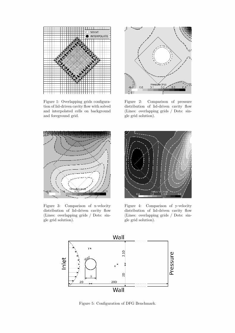
Figure 1: Overlapping grids configura-tion of lid-driven cavity flow with solvedand interpolated cells on backgroundand foreground grid.

Figure 2: Comparison of pressuredistribution of lid-driven cavity flow(Lines: overlapping grids / Dots: sin-gle grid solution).

Figure 3: Comparison of x-velocitydistribution of lid-driven cavity flow(Lines: overlapping grids / Dots: sin-gle grid solution).

Figure 4: Comparison of y-velocitydistribution of lid-driven cavity flow(Lines: overlapping grids / Dots: sin-gle grid solution).

Figure 5: Configuration of DFG Benchmark.

Figure 6: Single computational grid and overlapping grid configuration (Level 1).

Figure 7: Overlapping status on foreground and background cells (Level 1).

Figure 8: Comparison of pressure distributionof grid level 1 for channel flow (Lines: over-lapping grids / Dots: single grid).

Figure 9: Comparison of pressure distributionof grid level 2 for channel flow (Lines: over-lapping grids / Dots: single grid).

Figure 10: Comparison of pressure distribu-tion of grid level 3 for channel flow (Lines:overlapping grids / Dots: single grid).

Figure 11: Comparison x-velocity of grid level3 for channel flow (Lines: overlapping grids /Dots: single grid).

Figure 12: Comparison of y-velocity of gridlevel 3 for channel flow (Lines: overlappinggrids / Dots: single grid).

Figure 13: Streamline plot of grid level 3 ofchannel flow (overlapping grids configuration).

Figure 14: Drag coefficient of single and over-lapping grids configuration.

Figure 15: Lift coefficient of single and over-lapping grids configuration.

Numerical Assessment of a BEM-based Approach for theAnalysis of Ducted Propulsors

Danilo Calcagni, Luca Greco, Francesco SalvatoreINSEAN, Rome (Italy)

d.calcagni@insean.it

1 Introduction

Ducted propulsors are characterized by a screw propeller fit inside an annular airfoil (duct ornozzle). With respect to conventional open screw propellers, they yield an increase of thrustand efficiency at low values of the advance coefficient if an accelerating duct is used, whereasthe risk of blade cavitation is reduced in case of a decelerating duct. The mutual interactionbetween propeller and duct is very complex and is characterized by viscosity driven phenomenasuch as the interaction of blade tip with duct boundary layer in the gap region, the drag ex-erted on duct surface and, in many cases, the thick duct trailing edge emanating a thick viscouswake. Nevertheless, an inviscid approach is suitable to describe global interactional phenomenarelated mainly to vorticity and 3D effects more than viscosity. These include propeller inflowmodifications due to the duct and duct circulation generation induced by the rotating blades.Among inviscid (potential) approaches for the numerical analysis of ducted propellers, exam-ples of full BEM or BEM-vortex lattice are given in [4], [6] and [1] coupled with semi-empiricalmodels to address critical issues such as gap flow and flow separation induced by thick ducttrailing edge. whereas an exact description of viscous phenomena characterizing duct/bladeinteraction requires viscous flow models based on the solution of Navier-Stokes equations (see,for example, [12]).The present paper proposes a Boundary Element Method–based formulation to address hydro-dynamic analysis of ducted propellers. The methodology is in the framework of preliminary de-sign and optimization-oriented numerical tools, and is the object of a long-term research activityat INSEAN for the development of a hybrid RANSE/BEM approach to analyse hull/propulsorinteraction for open screw and ducted propellers. The theoretical and computational BEMapproach proposed here is valid for inviscid flows around three-dimensional bodies in arbitrarymotion. A formulation for open screw propellers is extended to ducted propulsors. In fact,the inclusion of the duct into the BEM simulations is very relevant, especially at low values ofthe advance coefficient, due to its impact on propeller performance. In order to investigate thecapabilities of a purely inviscid flow solver to address ducted propellers performance in theirtypical working conditions (low advance coefficient) and to avoid the uncertainties related tosemiempirical models, no gap flow semi-empirical modelling will be included in the analysis.Numerical results of the BEM code will be assessed and discussed against available experimen-tal data.Finally, sheet cavitation modelling for ducted propellers will be addressed based on the extensionof previous works by the authors (see, e.g., [10]).

2 Theoretical Model: Boundary Integral Formulation

Starting from a formulation valid for single propellers in cavitating and non-cavitating flows, aboundary integral formulation valid for inviscid potential flows around lifting/thrusting bodiesin arbitrary motion has been extended to describe complex configurations with rotating and

fixed parts using a time-accurate numerical scheme for unsteady flows.In the present model, an isolated ducted propulsor in a prescribed incoming flow vI is consid-ered, whereas no interaction between the propulsor and the hull is taken into account. Assumingthat the fluid is inviscid and irrotational, the perturbation velocity v may be expressed in termsof a scalar potential as v = ∇ϕ.The total velocity field can then be expressed as following q = vI + ∇ϕ, where vI has differentexpressions to describe inflow to rotating and non-rotating parts (i.e., blades or duct).Both open water and behind-hull conditions can be addressed: both a constant velocity distri-bution in the former case, and a velocity distribution corresponding to the hull-induced effectivewake in the latter can be included in the inflow.Assuming the flow is incompressible and recalling v = ∇ϕ, the continuity equation reduces tothe Laplace equation for the velocity potential ∇2ϕ = 0.The solution of the Laplace equation for ϕ is obtained here through a boundary integral for-mulation. A classical approach based on the third Green identity yields for an arbitrary pointx immersed into the fluid

E(x)ϕ(x) =∮S

B

(∂ϕ

∂nG− ϕ∂G

∂n

)dS(y) −

∫S

W

∆ϕGdS(y) (1)

where SB groups propeller, hub and nozzle surface, whereas SW collects the potential wakes(zero-thickness vortical layers) emanated from each lifting/thrusting body, i.e.blades and ducttrailing edge (see, e.g., [9]) and represent a discontinuity surface for the velocity potential.Vector n is the unit normal to SB and SW . Quantities G = −1/4π‖x− y‖ and ∂G/∂n denote,respectively, unit source and unit dipole in the unbounded three-dimensional space, whereasE(x) is a domain function whose value is 1 if the point x is outside the body surface, andE(x) = 1/2 if x lies on the body surface.The Laplace equation for the velocity potential is completed by boundary conditions on SB andSW . Impermeability condition on SB yields q · n = 0, thus relating ∂ϕ/∂n to the prescribedvI . Continuity of both pressure and of the normal component of the perturbation velocity isimposed on the wakes yielding, through mass and momentum conservation laws, that ∆ϕ isconstant following wake particles. A further condition on ϕ is required in order to assure that nofinite pressure jump may exist at the body trailing edge (Kutta condition, see e.g., [8]). In thepresent analysis propeller wake surface and nozzle wake surface are prescribed using analyticalgeometry descriptions.Finally, a sheet cavitation model has been developed in the past for open screw propellers (see,e.g.[10]) and is suitable to address sheet cavitation prediction on ducted propellers blades asfar as viscosity driven phenomena in the gap between blades and duct are slightly influencingcavitation appearance on blades surface. If cavitation occours, the impermeability boundarycondition needs to be reformulated. The present approach is limited to address sheet cavitationappearances on lifting surfaces (blades and duct). The cavity is assumed to be a thin layerattached to the solid surface and originating in the leading edge region. Detail of this modelare not given here and may be found in [10].

3 Numerical Solution Procedure

The numerical solution of the integral equation for the velocity potential is obtained herethrough a boundary element method (BEM) following an approach described in [3] for anisolated propeller and [2] for rotating/fixed interacting components. The proposed approach isvalid for the general case of a ducted propeller in unsteady flow conditions and is based on atime-marching solution of the flow around rotating and non-rotating parts in relative motion.

As far as uniform inflow conditions are considered, the axisymmetry of the problem can beexploited in order to reduce computational costs. In a frame of reference fixed to propellerblades, blade/duct interaction is a steady phenomena if a 1/Nb duct sector corresponding toa reference blade is considered. Considering a duct reference sector rigidly rotating with thereference blade, then the solution on the other duct sectors is obtained by imposing periodicity.The blade wake SW is built as helicoidal surface emanating from each blade trailing edge withprescribed pitch based on blade pitch and the unperturbed onset flow pitch. In the rotatingframe of reference, the duct wake is built as an helicoidal surface with the pitch correspondingto the unperturbed onset flow pitch and constant radius. Both blade and nozzle wakes can bestretched radially to take into account for the contraction of propeller-induced slipstream andfor the shape of the inner duct surface downstream the propeller.

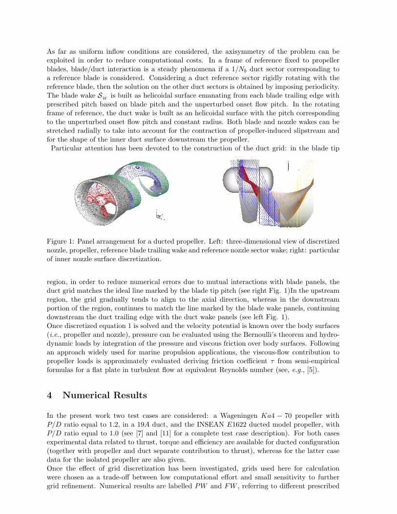
Particular attention has been devoted to the construction of the duct grid: in the blade tip

Figure 1: Panel arrangement for a ducted propeller. Left: three-dimensional view of discretizednozzle, propeller, reference blade trailing wake and reference nozzle sector wake; right: particularof inner nozzle surface discretization.

region, in order to reduce numerical errors due to mutual interactions with blade panels, theduct grid matches the ideal line marked by the blade tip pitch (see right Fig. 1)In the upstreamregion, the grid gradually tends to align to the axial direction, whereas in the downstreamportion of the region, continues to match the line marked by the blade wake panels, continuingdownstream the duct trailing edge with the duct wake panels (see left Fig. 1).Once discretized equation 1 is solved and the velocity potential is known over the body surfaces(i.e., propeller and nozzle), pressure can be evaluated using the Bernoulli’s theorem and hydro-dynamic loads by integration of the pressure and viscous friction over body surfaces. Followingan approach widely used for marine propulsion applications, the viscous-flow contribution topropeller loads is approximately evaluated deriving friction coefficient τ from semi-empiricalformulas for a flat plate in turbulent flow at equivalent Reynolds number (see, e.g., [5]).

4 Numerical Results

In the present work two test cases are considered: a Wageningen Ka4 − 70 propeller withP/D ratio equal to 1.2, in a 19A duct, and the INSEAN E1622 ducted model propeller, withP/D ratio equal to 1.0 (see [7] and [11] for a complete test case description). For both casesexperimental data related to thrust, torque and efficiency are available for ducted configuration(together with propeller and duct separate contribution to thrust), whereas for the latter casedata for the isolated propeller are also given.Once the effect of grid discretization has been investigated, grids used here for calculationwere chosen as a trade-off between low computational effort and small sensitivity to furthergrid refinement. Numerical results are labelled PW and FW , referring to different prescribed

propeller wakes geometries; the first is a simple helicoidal shape built as described in sec. 3,whereas the second is obtained through a trailing wake alignement tecnique for the isolatedpropeller. The use of an isolated propeller configuration for the evaluation of the flow-alignedwake shape is, as a first approximation, justified by a reduction of computational costs and bythe fact that propeller wake shape is largely dominated by blade loading distribution instead ofduct circulation, expecially at low advance coefficients.

In figure 2 comparison between experimental data and numerical results is shown for the

Figure 2: Ka4-70 in duct 19A: thrust, torque and efficiency. Left: blade and duct contributionto thrust. Right: total thrust, torque and efficiency. Comparison between numerical resultsand experimental data.

Ka4 − 70 case; total thrust (duct and propeller) as well as separate contributions to thrustfrom duct and propeller are shown. Significant discrepancies can be found at high values of theadvance coefficient J . This can be explained considering that, in those working conditions, thepropeller is lightly loaded, hence its effect on the duct circulation is small. This yields that ducthydrodynamic loads are dominated by viscous drag (as indicated by negative duct thrust) thatis not accurately modelled in the present potential flow code. The presence of relevant viscousphenomena is confirmed by RANSE calculations on the same configuration (with a downstreamrudder) performed in [12].Note that the use of a free wake geometry instead of an helicoidal one, even if obtained forthe isolated propeller, improves the accuracy of results at low values of the advance coefficient(below 0.6), for both propeller and duct contribution to thrust, thus indicating that wake roll-upand contraction have a significant influence on the prediction of the flow around the duct forlow values of J .Considering J = 0.5, the FW predictions is compared to the PW ones in terms of pressurecoefficient CP acting both on the propeller and duct surfaces in fig.3. Significant differencies

Figure 3: Ka4-70 in duct 19A: numerical predictions of blade and duct pressure distribution atJ = 0.5. Left: prescribed blade wake PW ; right: free blade wake FW .

in the contours can be found only on duct surface. On the outer side, near the leading andthe trailing edge, a wider zone characterized by lower pressure values is predicted by the useof a prescribed helicoidal wake. In the duct inner side, differencies are mainly present in theregion where the propeller wake interacts with the duct surface. This interaction is strongerin the PW case for which no contraction, or wake roll-up is considered. These differencies inthe pressure distribution are responsible for a lower duct thrust prediction when a flow-alignedwake is not included in the model. Note that, the use of a free wake slightly influences predictedpropeller thrust contribution, whereas it greatly improves predicted duct thrust.In order to assess the proposed methodology for an isolated propeller considering the particularblade geometries typical of ducted propellers, in fig.4 numerical estimation of thrust torqueand efficiency is compared to experimental data for the INSEAN E1622 isolated propeller case.Experimental results were obtained either at INSEAN and UPM for different Reynolds numbersin accordance with ITTC procedures (see [11]). A good agreement is shown for all values of the

Figure 4: E1622 isolated propeller: thrust, torque and efficiency. Comparison between numericalresults and experimental data.

advance coefficient. Propeller efficiency is slightly underpredicted at high values of J , due toslight underprediction of KT . Next, in fig.5 the ducted propeller configuration is considered andPW/FW comparison is performed. At high values of J (above 0.5) the total thrust coefficient

Figure 5: E1622 in duct: thrust, torque and efficiency. Left: blade and duct contribution tothrust. Right: total thrust, torque and efficiency. Comparison between numerical results andexperimental data.

is overpredicted by using any wake shape, and this is mainly due to an overestimation of theduct contribution. This confirms the results obtained for the Ka4− 70 test case. At low valuesof J , the propeller contribution to thrust is overpredicted, whereas the duct contribution isunderpredicted. As far as duct contribution to thrust is concerned, the use of a flow-alignedwake improves numerical predictions, whereas propeller thrust is generally not influenced (withslight overprediction of experimental data at low values of J) if a free wake model is included.

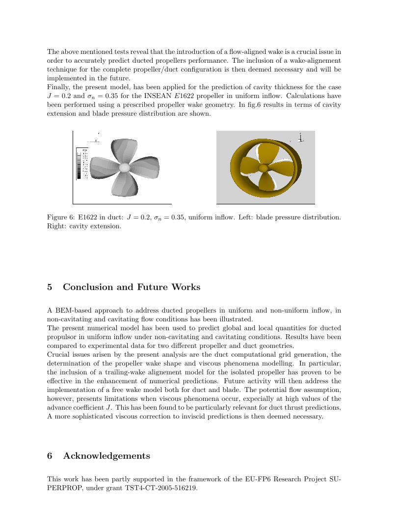
The above mentioned tests reveal that the introduction of a flow-aligned wake is a crucial issue inorder to accurately predict ducted propellers performance. The inclusion of a wake-alignementtechnique for the complete propeller/duct configuration is then deemed necessary and will beimplemented in the future.Finally, the present model, has been applied for the prediction of cavity thickness for the caseJ = 0.2 and σn = 0.35 for the INSEAN E1622 propeller in uniform inflow. Calculations havebeen performed using a prescribed propeller wake geometry. In fig.6 results in terms of cavityextension and blade pressure distribution are shown.

Figure 6: E1622 in duct: J = 0.2, σn = 0.35, uniform inflow. Left: blade pressure distribution.Right: cavity extension.

5 Conclusion and Future Works

A BEM-based approach to address ducted propellers in uniform and non-uniform inflow, innon-cavitating and cavitating flow conditions has been illustrated.The present numerical model has been used to predict global and local quantities for ductedpropulsor in uniform inflow under non-cavitating and cavitating conditions. Results have beencompared to experimental data for two different propeller and duct geometries.Crucial issues arisen by the present analysis are the duct computational grid generation, thedetermination of the propeller wake shape and viscous phenomena modelling. In particular,the inclusion of a trailing-wake alignement model for the isolated propeller has proven to beeffective in the enhancement of numerical predictions. Future activity will then address theimplementation of a free wake model both for duct and blade. The potential flow assumption,however, presents limitations when viscous phenomena occur, expecially at high values of theadvance coefficient J . This has been found to be particularly relevant for duct thrust predictions.A more sophisticated viscous correction to inviscid predictions is then deemed necessary.

6 Acknowledgements

This work has been partly supported in the framework of the EU-FP6 Research Project SU-PERPROP, under grant TST4-CT-2005-516219.

References

[1] Baltazar, J., Falcao de Campos, J.A.C. (2009). “On the Modelling of the Flow in DuctedPropellers with a Panel Method,” First International Symposium on Marine Propulsors,SMP09, Trondheim (Norway), June 2009.

[2] Greco, L., Colombo, C., Salvatore, F., Felli, M. (2006). “An Unsteady Inviscid-Flow Modelto Study Podded Propulsors Hydrodynamics,” Second International Conference on Tech-nological Advances in Podded Propulsion, Brest (France), October 2006.

[3] Greco, L., Salvatore, F., Di Felice, F. (2004) “Validation of a Quasi–potential Flow Modelfor the Analysis of Marine Propellers Wake”, Twenty-fifth ONR Symposium on NavalHydrodynamics, St. John’s, Newfoundland (Canada).

[4] Kerwin, J.E., Kinnas, S.A., Lee, J.-T., Shih, W.-Z. (1987) “A surface panel method for thehydrodynamic analysis of ducted propellers”, Transaction SNAME, vol. 95, 1987.

[5] Harvald, S. A. (1992). Resistance and Propulsion of Ships. Wiley Interscience Pubblication,New York, USA.

[6] Hughes, M.J. (1997). “Implementation of a Special Procedure for Modeling the Tip Clear-ance Flow in a Panel Method for Ducted Propellers,” Propellers/Shafting ’97 Symposium,Virginia Beach (USA).

[7] Kuiper, G. (1992). The Wageningen Propeller Series. Marin Pubblication 92-001.

[8] Morino, L, Chen, L.T. and Suciu, E. (1975), “Steady and Oscillatory Subsonic and Su-personic Aerodynamics Around Complex Configurations,” AIAA Journal, Vol. 13, pp.368–374.

[9] Morino, L. (1993), “Boundary Integral Equations in Aerodynamics,” Applied MechanicsReviews, Vol. 46, No. 8, pp. 445-466.

[10] Salvatore, F., Testa, C., Ianniello, S., Pereira, F. (2006). “Theoretical Modelling of Un-steady Cavitation and Induced Noise,” Proceedings of CAV 2006 Symposium, Wageningen(The Netherlands) September 2006.

[11] Salvatore, F., Calcagni, D., Greco, L. (2006). “Ducted propeller performance analysis usinga boundary element model,” INSEAN Technical Report / 2006-083, 2006.

[12] Sanchez-Caja, A., Pylkkanen J.V., Sipila, T.P. (2008) “Simulation of the IncompressibleViscous Flow around Ducted Propellers with Rudders Using a RANSE Solver,” 27th Sym-posium on Naval Hydrodynamics, Seoul (Korea), October 2008.

Modification of the rudder geometry for energy efficiency improvement on ships

Alejandro Caldas Collazo a.caldas@vicusdt.com

Adrián Sarasquete Fernándeza.sarasquete@vicusdt.com

Vicus Desarrollos Tecnológicos S.L.- Vigo - Spain

1. Introduction

The main role of the rudder in most of the ships is to act as a steering device, but at the same time it also performs a very significant, but not so well known, task as an energy recovery device, interacting with the water flow leaving the propeller.

Vicus Desarrollos Tecnológicos S.L., in cooperation with Baliño S.A. and Progener Steering Systems, are carrying out a joint research project focused on the improvement of the propeller-rudder interaction mainly for fishing vessels. Today the fuel consumption is one of the major costs faced by any fleet, specifically determinant for fishing fleets, and any decrease in the consumption will be welcome by shipowners. The main goal is improving the energy recovery through the rudder so can increase the energy efficiency of the ship with a quite low investment since the shipowner only has to substitute the rudder blade. Our objective is to do this through numerical methods previously calibrated via experiments; for the calculation of the propeller we have used the panel code PPB from HSVA and for the rudder calculations and grid generation we have used Star CCM + from CD-Adapco.

2. Physical Behaviour

Complex interaction phenomena occurs among propeller, rudder and hull, affecting `propulsive efficiency in different ways (thrust deduction, wake fraction,...). In this paper we will focus only on the propeller losses, which can be classified as: axial, friction and rotational losses. In the present work we mainly deal with rotational looses since a percentage of them are already recovered on a conventional rudder. The propeller accelerate the water flow inducing a velocity field composed of axial, radial and tangential velocities. Our goal is to adapt the geometry of the rudder blade in order to increase the recovery of these rotational losses.

Fig 1. Lift and drag forces in rudder profile

As it can be seen in Fig 1 our goal is to modify the lift and drag forces on the rudder in such a way that the resultant longitudinal force is maximum if it points forward (or minimum if it points aftwards).

3. Mathematical models and Numerical Methods

Although in these lines, we focus our efforts on calculating the velocity and pressure field configuration close to the rudder, the calculation should also take into account what happens in hull and propeller as these calculations influence the operation condition of the rudder. If we perform a calculation of the forces on different rudder geometries with the whole set taking into account the deformation of the free surface and complete hull-propeller-rudder interaction, it leads to huge computation time and therefore it wouldn't be an operational method for the hydrodynamic design of the rudder since several cases must be analyzed. Instead of this, we choose a set of of simplified unidirectional coupled models, at first less accurate but enough for our purposes. Our first simplification is to decompose our problem into three distinct sub zones with their sub mathematical models and associated sub numerical methods : The hull, the propeller and the rudder.

This simplification, which may be somewhat questionable, makes unidirectional the flow of information, ie data will go from hull to the propeller and from the propeller to rudder but not the reverse. In fact, we know for certain that this is not true as the functioning of the propeller modifies the wake field, and moreover the rudder affects the propeller loading by changing its operating point; as we said at first we are not going to take this into account. Despite this, we believe that based on the results of the validation work, this decomposition is useful for the redesign the rudder geometry and suitable to carry out our calculations in relative short times with enough accuracy.

4. Propeller

In general, it is an usual practice to carry out the propeller calculation using models that neglecting the viscosity and solving the Laplace equation. This is much faster than solving the whole Navier Stokes Equations (less equations and less grid points), with enough good results for the calculation of the propeller in steady condition. The solution of this mathematical model is carried out applying a Boundary Element Method implemented in PPB code from HSVA (Streckwall).

5. Rudder

For the rudder we chose a model without free surface but taking into account diffusive terms in our differential equations as we are in a zone where diffusive terms are quite important. So we will try to solve Reynolds Averaged Navier Stokes Equations with two equations for k and coupled with a log wall law. For the solver we have chosen a segregated approximation for velocity and pressure and a steady temporal discretization.

6. Case 1 : Molland and Turnock Experiments

To assess and calibrate our models we have used some of the test cases about propeller-rudder interaction published by Molland and Turnock and carried out in the wind tunnel. After that we used this model for the design of a new rudder for an operating tuna vessel.We compared our results for two load conditions on one of the test cases carried out by Molland and Turnock [5] . In the table 1, we show the main particulars of the rudder, relative position between propeller and rudder and propeller operating point.

Span (m) 1Root Chord (m) 0,667Tip Chord (m) 0,667Z/D 0,75Y/D 0X/D 0,52V (m/s) 10

n1 (rpm) 1433J 1 0,52n2 (rpm) 2079J 2 0,36

Table 1 Characteristics The results of the comparison are presented in the table 2 below.

Case 1Cells Ct1605224 7,2E-3644559 8,1E-3253645 9,0E-3

Experimental 7,0E-3

Case 2 Cells Ct1605224 -4,4E-02644559 -4,1E-02253645 -4,0E-02Experimental -4,6E-02

Table 2 Calculation results

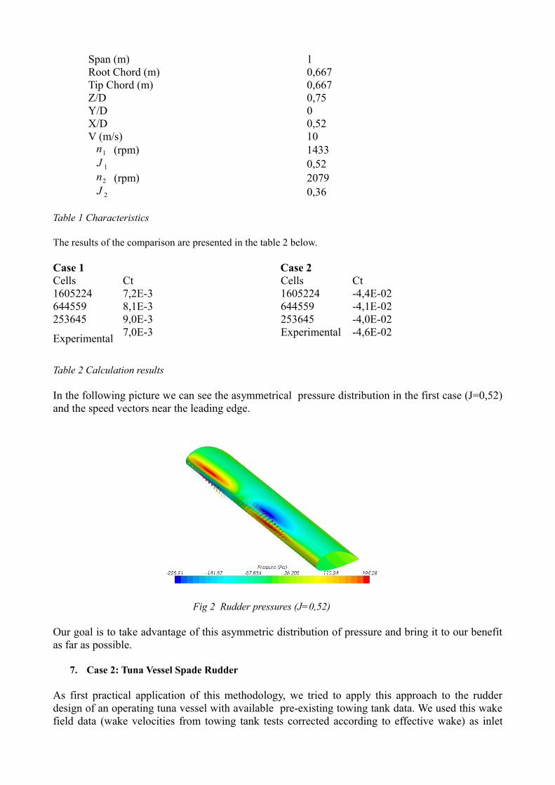
In the following picture we can see the asymmetrical pressure distribution in the first case (J=0,52) and the speed vectors near the leading edge.

Fig 2 Rudder pressures (J=0,52)

Our goal is to take advantage of this asymmetric distribution of pressure and bring it to our benefit as far as possible.

7. Case 2: Tuna Vessel Spade Rudder

As first practical application of this methodology, we tried to apply this approach to the rudder design of an operating tuna vessel with available pre-existing towing tank data. We used this wake field data (wake velocities from towing tank tests corrected according to effective wake) as inlet

boundary conditions inside PPB. After this we took PPB outlet velocities as inlet in a RANSE calculation (Star CCM+ ), in the same way exposed in the above sections. We carried out this calculation for the original rudder:

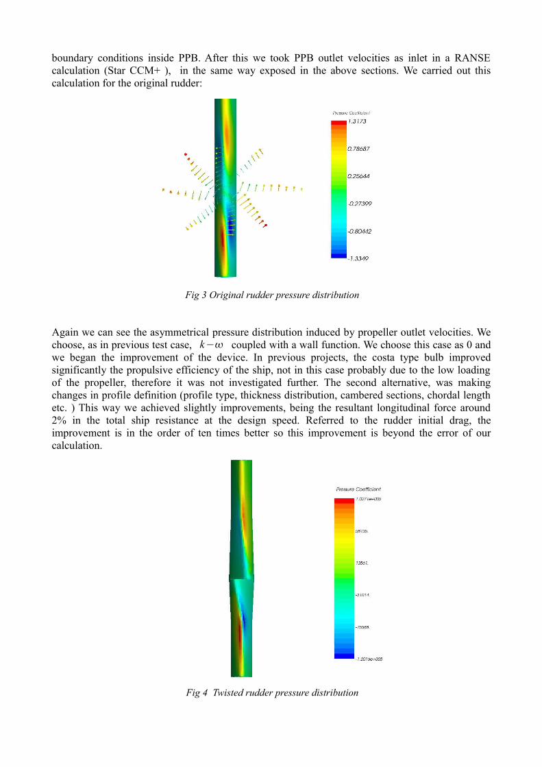
Fig 3 Original rudder pressure distribution

Again we can see the asymmetrical pressure distribution induced by propeller outlet velocities. We choose, as in previous test case, k− coupled with a wall function. We choose this case as 0 and we began the improvement of the device. In previous projects, the costa type bulb improved significantly the propulsive efficiency of the ship, not in this case probably due to the low loading of the propeller, therefore it was not investigated further. The second alternative, was making changes in profile definition (profile type, thickness distribution, cambered sections, chordal length etc. ) This way we achieved slightly improvements, being the resultant longitudinal force around 2% in the total ship resistance at the design speed. Referred to the rudder initial drag, the improvement is in the order of ten times better so this improvement is beyond the error of our calculation.

Fig 4 Twisted rudder pressure distribution

Finally, we tried with a pair of thrusting fins; the combination of these two solutions gave us the best improvement around 4% to the hull towing force. There is a relationship between the rotational losses of the propeller and the effectiveness of the rudder as energy recovery device. These rotational losses are mainly related to the load of our propeller, advance ratio and blade number..

Fig 5 Cambered+Fins

8. Conclusion and Further work

In the above lines we have proposed a design method for improving the energy efficiency of rudders, using an approximate calculation method. We know in advance that we have incurred in inaccuracies due to the approximated mathematical model used, but after comparing with experimental results (Molland - Turnock experiments), we also know that the error introduced by this model inaccuracies will be lower than the improvement achieved. The next step will be adding another calculation phase for analyzing the best designs coupling propeller and rudder in a single RANSE model.

References

[1]Bertram, V. Practical ship hydrodynamics. Butterwoth-Heinemann. 2002

[2]Carlton, J. Marine propellers and Propulsion. 2nd Edition. Butterworth-Heinemann 2007,

[3]Li, Da-Quing. Investigation on Propeller-rudder interaction by numerical methods. PhD thesis. Chalmers University of Technology.

[4]Ferziger, J.H., Perić, M. Computational Methods for fluid dynamics. Springer. 2000

[5]Molland, A. F. and Turnock, S.R. Marine Rudders and Control Surfaces. Butterworth-Heinemann 2007.

[6]Söding, H. Limits of potential theory in rudder flow predictions. Twenty-Second Symposium on Naval Hydrodynamics. Washington, D.C. 1998

[7]Stierman E.J. The influence of the rudder on the propulsive performance of ships Part I & II. International Shipbuilding Progress, 36, Nº 407 (1989) pp 303-334 y Nº 408 (1989) pp 405-435

[8]Streckwall H. Rudder Cavitation. Numerical Analysis and Shape Optimization. STG CFD in ship Design. Hamburg. 2007

[9]Tetsuhi Hoshino et Al. Development of high performance stator fin by using advanced panel method. Mitsubishi Heavy Industries Technical Review. Vol 41 Nº6. 2004

[10]Vorhoelter, H., Krueger,S..Optimization of appendages using RANS-CFD Methods, Numerical Towing Tank Symposium, Hamburg 2007

Numerical study of a submergedtwo-dimensional hydrofoil using different solvers

Andrea Califanocalifano@ntnu.no

Department of Marine Technology - NTNURolls-Royce University Technology Center ’Performance in a Seaway’

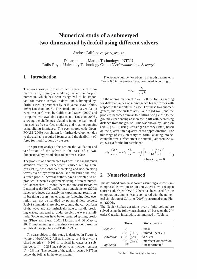
1 Introduction

This work was performed in the framework of a nu-merical study aiming at modeling the ventilation phe-nomenon, which has been recognized to be impor-tant for marine screws, rudders and submerged hy-drofoils (see experiments by Nishiyama, 1961; Shiba,1953; Koushan, 2006). The simulation of a ventilationevent was performed by Califano and Steen (2009) andcompared with available experiments (Koushan, 2006),showing the challenges related to its numerical model-ing, such as free surface modeling and rotating domainsusing sliding interfaces. The open source code Open-FOAM (2009) was chosen for further development dueto the available required features and the flexibility of-fered for modifications by the user.

The present analysis focuses on the validation andverification of the solver in the case of a two-dimensional hydrofoil close to the free surface.

The problem of a submerged hydrofoil has caught muchattention after the experiments carried out by Dun-can (1983), who observed breaking and non-breakingwaves over a hydrofoil model and measured the free-surface profile. Several authors have attempted to re-produce Duncan’s experiments using different numer-ical approaches. Among them, the inviscid BEMs byLandrini et al. (1999) and Faltinsen and Semenov (2008)have reproduced accurately the experimental results un-til breaking occurs. After that, the following flow evo-lution can not be handled by potential flow solvers.RANS simulations are able to capture the correct formof the wave and are intrinsically able to handle break-ing waves, but tend to under-predict the wave ampli-tude. Some authors have better captured spilling break-ers (Rhee and Stern, 2002; Muscari and Di Mascio,2003) implementing a breaking-wave model based onempirical data (Cointe and Tulin, 1994).

The case object of this study is depicted in Figure 1,where a NACA0012 foil at incidence of 5 deg with achord lengthc = 0.203 m is fixed in water at a sub-mergenceh = 0.261 m, subject to an incident currentU = 0.8 m/s. The bottom of the tank is located 0.175 mbelow the foil, as in the experiments.

The Froude number based onh as length parameter isFnh = 0.5 in the present case, computed according to:

Fnh =U√g h

In the approximation ofFnh → 0 the foil is exertingfor different values of submergence higher forces withrespect to the infinite fluid case. For these low submer-gences, the free surface acts like a rigid wall, and theproblem becomes similar to a lifting wing close to theground, experiencing an increase in lift with decreasingdistance from the ground. This was shown by Faltinsen(2005,§ 6.8.1) using Weissinger’s theory (1947) basedon the quarter-three-quarter-chord approximation. Forthis range ofFnh, an analytical formula taking into ac-count the free-surface effect is derived (Faltinsen, 2005,eq. 6.143) for the lift coefficient:

CL

(

h

c

)

= CL

(

h

c= ∞

) [

1 +1

16

( c

h

)2]

whenFnh → 0

(1)

2 Numerical method

The described problem is solved assuming a viscous, in-compressible, two-phase (air and water) flow. The opensource code OpenFOAM (2009) has been used for thecomputations, and its results compared with the numer-ical simulation of Califano (2008), performed using Flu-ent (2006).The Navier Stokes equations over a finite volume aresolved using the following schemes, all based on the 2nd

order Gaussian integration, summarized in Table 1:

Term Discretization

Gradient ∇ linear

Convection∇ · (ρφU) limited linearV 1∇ · (φγ) vanLeer∇ · (φrbγ) interfaceCompression

Laplacian ∇2 linear corrected

Table 1: Numerical schemes

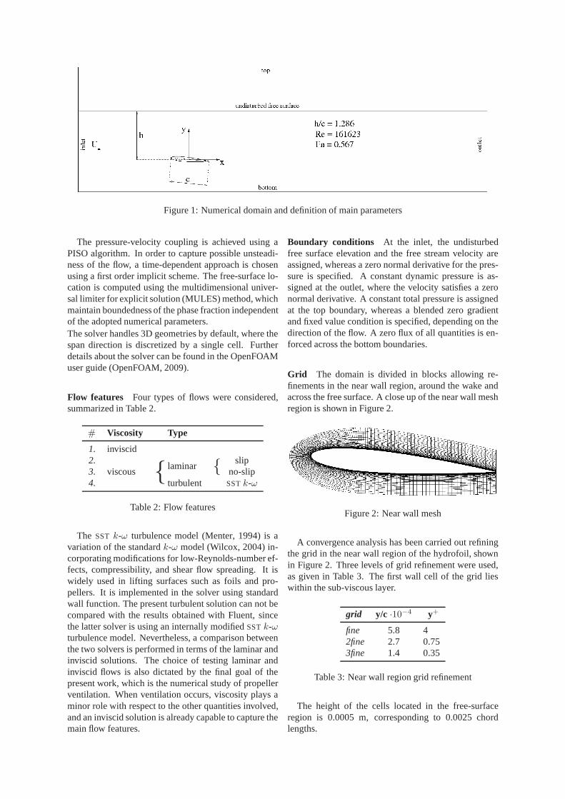
Figure 1: Numerical domain and definition of main parameters

The pressure-velocity coupling is achieved using aPISO algorithm. In order to capture possible unsteadi-ness of the flow, a time-dependent approach is chosenusing a first order implicit scheme. The free-surface lo-cation is computed using the multidimensional univer-sal limiter for explicit solution (MULES) method, whichmaintain boundedness of the phase fraction independentof the adopted numerical parameters.The solver handles 3D geometries by default, where thespan direction is discretized by a single cell. Furtherdetails about the solver can be found in the OpenFOAMuser guide (OpenFOAM, 2009).

Flow features Four types of flows were considered,summarized in Table 2.

# Viscosity Type

1. inviscid2.

viscous laminar slip3. no-slip4. turbulent SSTk-ω

Table 2: Flow features

The SST k-ω turbulence model (Menter, 1994) is avariation of the standardk-ω model (Wilcox, 2004) in-corporating modifications for low-Reynolds-number ef-fects, compressibility, and shear flow spreading. It iswidely used in lifting surfaces such as foils and pro-pellers. It is implemented in the solver using standardwall function. The present turbulent solution can not becompared with the results obtained with Fluent, sincethe latter solver is using an internally modifiedSSTk-ωturbulence model. Nevertheless, a comparison betweenthe two solvers is performed in terms of the laminar andinviscid solutions. The choice of testing laminar andinviscid flows is also dictated by the final goal of thepresent work, which is the numerical study of propellerventilation. When ventilation occurs, viscosity plays aminor role with respect to the other quantities involved,and an inviscid solution is already capable to capture themain flow features.

Boundary conditions At the inlet, the undisturbedfree surface elevation and the free stream velocity areassigned, whereas a zero normal derivative for the pres-sure is specified. A constant dynamic pressure is as-signed at the outlet, where the velocity satisfies a zeronormal derivative. A constant total pressure is assignedat the top boundary, whereas a blended zero gradientand fixed value condition is specified, depending on thedirection of the flow. A zero flux of all quantities is en-forced across the bottom boundaries.

Grid The domain is divided in blocks allowing re-finements in the near wall region, around the wake andacross the free surface. A close up of the near wall meshregion is shown in Figure 2.

Figure 2: Near wall mesh

A convergence analysis has been carried out refiningthe grid in the near wall region of the hydrofoil, shownin Figure 2. Three levels of grid refinement were used,as given in Table 3. The first wall cell of the grid lieswithin the sub-viscous layer.

grid y/c ·10−4 y+

fine 5.8 42fine 2.7 0.753fine 1.4 0.35

Table 3: Near wall region grid refinement

The height of the cells located in the free-surfaceregion is 0.0005 m, corresponding to 0.0025 chordlengths.

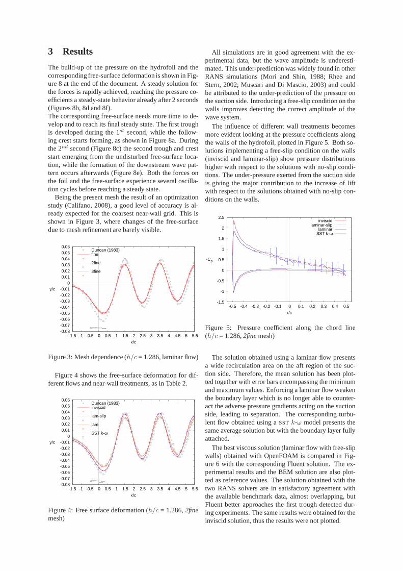
3 Results

The build-up of the pressure on the hydrofoil and thecorresponding free-surface deformation is shown in Fig-ure 8 at the end of the document. A steady solution forthe forces is rapidly achieved, reaching the pressure co-efficients a steady-state behavior already after 2 seconds(Figures 8b, 8d and 8f).The corresponding free-surface needs more time to de-velop and to reach its final steady state. The first troughis developed during the 1st second, while the follow-ing crest starts forming, as shown in Figure 8a. Duringthe 2nd second (Figure 8c) the second trough and creststart emerging from the undisturbed free-surface loca-tion, while the formation of the downstream wave pat-tern occurs afterwards (Figure 8e). Both the forces onthe foil and the free-surface experience several oscilla-tion cycles before reaching a steady state.

Being the present mesh the result of an optimizationstudy (Califano, 2008), a good level of accuracy is al-ready expected for the coarsest near-wall grid. This isshown in Figure 3, where changes of the free-surfacedue to mesh refinement are barely visible.

-0.08-0.07-0.06-0.05-0.04-0.03-0.02-0.01

0 0.01 0.02 0.03 0.04 0.05 0.06

-1.5 -1 -0.5 0 0.5 1 1.5 2 2.5 3 3.5 4 4.5 5 5.5

y/c

x/c

Duncan (1983)fine 2fine 3fine

Figure 3: Mesh dependence (h/c = 1.286, laminar flow)

Figure 4 shows the free-surface deformation for dif-ferent flows and near-wall treatments, as in Table 2.

-0.08-0.07-0.06-0.05-0.04-0.03-0.02-0.01

0 0.01 0.02 0.03 0.04 0.05 0.06

-1.5 -1 -0.5 0 0.5 1 1.5 2 2.5 3 3.5 4 4.5 5 5.5

y/c

x/c

Duncan (1983)inviscid lam-slip lam SST k-ω

Figure 4: Free surface deformation (h/c = 1.286,2finemesh)

All simulations are in good agreement with the ex-perimental data, but the wave amplitude is underesti-mated. This under-prediction was widely found in otherRANS simulations (Mori and Shin, 1988; Rhee andStern, 2002; Muscari and Di Mascio, 2003) and couldbe attributed to the under-prediction of the pressure onthe suction side. Introducing a free-slip condition on thewalls improves detecting the correct amplitude of thewave system.

The influence of different wall treatments becomesmore evident looking at the pressure coefficients alongthe walls of the hydrofoil, plotted in Figure 5. Both so-lutions implementing a free-slip condition on the walls(inviscid and laminar-slip) show pressure distributionshigher with respect to the solutions with no-slip condi-tions. The under-pressure exerted from the suction sideis giving the major contribution to the increase of liftwith respect to the solutions obtained with no-slip con-ditions on the walls.

-1.5

-1

-0.5

0

0.5

1

1.5

2

2.5

-0.5 -0.4 -0.3 -0.2 -0.1 0 0.1 0.2 0.3 0.4 0.5

-Cp

x/c

inviscidlaminar-slip

laminarSST k-ω

Figure 5: Pressure coefficient along the chord line(h/c = 1.286,2finemesh)

The solution obtained using a laminar flow presentsa wide recirculation area on the aft region of the suc-tion side. Therefore, the mean solution has been plot-ted together with error bars encompassing the minimumand maximum values. Enforcing a laminar flow weakenthe boundary layer which is no longer able to counter-act the adverse pressure gradients acting on the suctionside, leading to separation. The corresponding turbu-lent flow obtained using aSST k-ω model presents thesame average solution but with the boundary layer fullyattached.

The best viscous solution (laminar flow with free-slipwalls) obtained with OpenFOAM is compared in Fig-ure 6 with the corresponding Fluent solution. The ex-perimental results and the BEM solution are also plot-ted as reference values. The solution obtained with thetwo RANS solvers are in satisfactory agreement withthe available benchmark data, almost overlapping, butFluent better approaches the first trough detected dur-ing experiments. The same results were obtained for theinviscid solution, thus the results were not plotted.

-0.08-0.07-0.06-0.05-0.04-0.03-0.02-0.01

0 0.01 0.02 0.03 0.04 0.05 0.06

-1.5 -1 -0.5 0 0.5 1 1.5 2 2.5 3 3.5 4 4.5 5 5.5

y/c

x/c

Duncan (1983)Landrini et al. (1999)Fluent, 2fine lam-slip

2fine lam-slip

Figure 6: Comparison of the free surface deformation(h/c = 1.286,2finemesh)

Figure 7 shows a comparison of the pressure coeffi-cient with Fluent calculations and the infinite fluid case,also reporting the corresponding lift coefficients. BothRANS solvers predict the same distribution, showingthe increase of pressure due to the presence of the free-surface, especially on the suction side, leading to higherforces exerted by the submerged hydrofoil with respectto the infinite fluid case.

-1.5

-1

-0.5

0

0.5

1

1.5

2

2.5

-0.5 -0.4 -0.3 -0.2 -0.1 0 0.1 0.2 0.3 0.4 0.5

-Cp

x/c

CL = 0.713CL = 0.705CL = 0.735CL = 0.595 h/c = ∞

h/c = 0.911h/c = 1.286h/c = 1.286, Fluent

Figure 7: Comparison of the pressure coefficient (2finemesh, laminar flow with free-slip walls)

The same figure shows the pressure coefficient for acase with shallower submergence,h = 0.185 m, cor-responding to a submergence ratioh/c = 0.911. Forthis shallower submergence the experiments by Duncan(1983) show a clear spilling breaking-wave condition,which is not attempted to capture with the present simu-lation. The converged pressure distribution for this fur-ther case is used to confirm that the wave system gener-ated above the hydrofoil requires higher energy in orderto attain the same flow speed (Tzabiras, 1997).

The ratio betweenCL and its infinite fluid value is1.18 and 1.24, respectively forh/c = 1.286 and 0.911.The corresponding values obtained using Equation 1 are1.04 and 1.08. Weissinger’s theory shows the correcttrend for the lift, which increases at low submergences,but present values are underestimated of about 13%.

This approximation fails to predict the surface-piercingcase (CL → ∞ whenh/c → 0) and is thus less accuratefor intermediate cases.

Table 4 summarizes the present results obtained forthe dimensionless first trough amplitudeη/c and the liftcoefficientCL, in terms of relative error with respect tothe experiments (Duncan, 1983) and the BEM solutionby Landrini et al. (1999), respectively. An increasinglift coefficient corresponds to a more accurate represen-tation of the free surface; the effect of different near wallconditions is also confirmed.

CL η/c

SSTk-ω

OpenFOAM -19.3% -19.4%

inviscid 1.0% -7.8%

laminar no-slip -16.4% -17.8%

slip 1.0% -7.8%

Fluent 2.1% -1.4%

Table 4: Relative error of the present solution with re-spect to the experiments (Duncan, 1983) and the BEMsolution (Landrini et al., 1999) (h/c = 1.286, 2finemesh)

The same table compares the results for the lami-nar flow using free-slip conditions for the two RANSsolvers. While both lift coefficients approach satisfacto-rily the BEM solution, OpenFOAM presents a larger de-viation in the first trough amplitude, as already pointedout in Figure 6. This large percent deviation corre-sponds to only 2 grid cells, and the difference amongthe solvers could be ascribed to the different schemesused to interpolate the interface between air and water.

4 Concluding remarks

A two-dimensional hydrofoil close to the free surfacehas been simulated using the open source code Open-FOAM and its results compared with those obtained us-ing the commercial code Fluent (Califano, 2008). Theobtained results have been validated by experiments(Duncan, 1983) and verified using three levels of near-wall grid refinement and with a BEM solver (Landriniet al., 1999).

The present converged analysis shows a satisfactoryagreement with the experimental results and the poten-tial flow solution, both in terms of free surface defor-mation and lift coefficient. The detection of the cor-rect wave amplitudes is improved introducing a free-slipcondition on the walls.

The two RANS solvers show an overall good agree-ment. The same pressure distribution is predicted alongthe hydrofoil, and the differences found in the free-surface deformation could be ascribed to the differentschemes the solvers use in order to interpolate the inter-face between air and water.

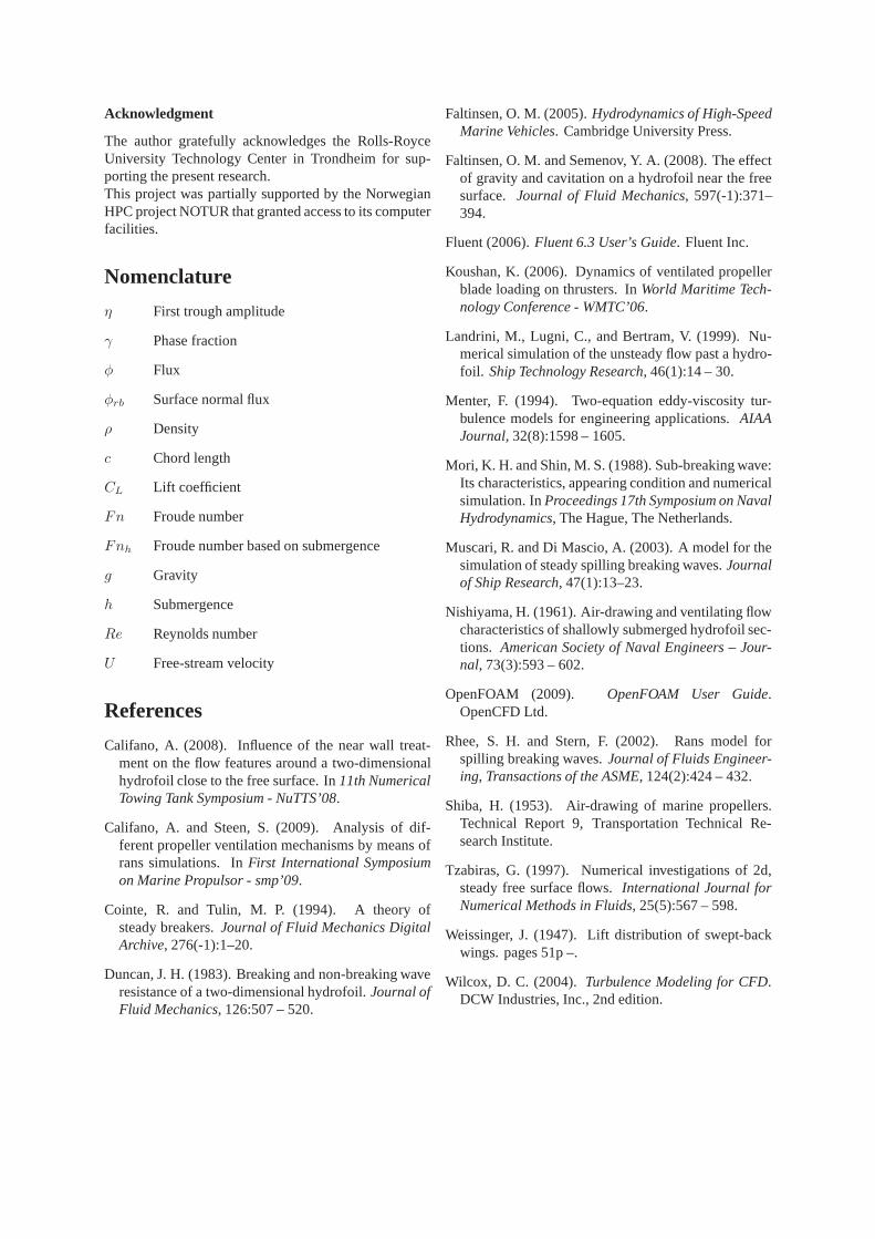
Acknowledgment

The author gratefully acknowledges the Rolls-RoyceUniversity Technology Center in Trondheim for sup-porting the present research.This project was partially supported by the NorwegianHPC project NOTUR that granted access to its computerfacilities.

Nomenclature

η First trough amplitude

γ Phase fraction

φ Flux

φrb Surface normal flux

ρ Density

c Chord length

CL Lift coefficient

Fn Froude number

Fnh Froude number based on submergence

g Gravity

h Submergence

Re Reynolds number

U Free-stream velocity

References

Califano, A. (2008). Influence of the near wall treat-ment on the flow features around a two-dimensionalhydrofoil close to the free surface. In11th NumericalTowing Tank Symposium - NuTTS’08.

Califano, A. and Steen, S. (2009). Analysis of dif-ferent propeller ventilation mechanisms by means ofrans simulations. InFirst International Symposiumon Marine Propulsor - smp’09.

Cointe, R. and Tulin, M. P. (1994). A theory ofsteady breakers.Journal of Fluid Mechanics DigitalArchive, 276(-1):1–20.

Duncan, J. H. (1983). Breaking and non-breaking waveresistance of a two-dimensional hydrofoil.Journal ofFluid Mechanics, 126:507 – 520.

Faltinsen, O. M. (2005).Hydrodynamics of High-SpeedMarine Vehicles. Cambridge University Press.

Faltinsen, O. M. and Semenov, Y. A. (2008). The effectof gravity and cavitation on a hydrofoil near the freesurface. Journal of Fluid Mechanics, 597(-1):371–394.

Fluent (2006).Fluent 6.3 User’s Guide. Fluent Inc.

Koushan, K. (2006). Dynamics of ventilated propellerblade loading on thrusters. InWorld Maritime Tech-nology Conference - WMTC’06.

Landrini, M., Lugni, C., and Bertram, V. (1999). Nu-merical simulation of the unsteady flow past a hydro-foil. Ship Technology Research, 46(1):14 – 30.

Menter, F. (1994). Two-equation eddy-viscosity tur-bulence models for engineering applications.AIAAJournal, 32(8):1598 – 1605.

Mori, K. H. and Shin, M. S. (1988). Sub-breaking wave:Its characteristics, appearing condition and numericalsimulation. InProceedings 17th Symposium on NavalHydrodynamics, The Hague, The Netherlands.

Muscari, R. and Di Mascio, A. (2003). A model for thesimulation of steady spilling breaking waves.Journalof Ship Research, 47(1):13–23.

Nishiyama, H. (1961). Air-drawing and ventilating flowcharacteristics of shallowly submerged hydrofoil sec-tions. American Society of Naval Engineers – Jour-nal, 73(3):593 – 602.

OpenFOAM (2009). OpenFOAM User Guide.OpenCFD Ltd.

Rhee, S. H. and Stern, F. (2002). Rans model forspilling breaking waves.Journal of Fluids Engineer-ing, Transactions of the ASME, 124(2):424 – 432.

Shiba, H. (1953). Air-drawing of marine propellers.Technical Report 9, Transportation Technical Re-search Institute.

Tzabiras, G. (1997). Numerical investigations of 2d,steady free surface flows.International Journal forNumerical Methods in Fluids, 25(5):567 – 598.

Weissinger, J. (1947). Lift distribution of swept-backwings. pages 51p –.

Wilcox, D. C. (2004). Turbulence Modeling for CFD.DCW Industries, Inc., 2nd edition.

-0.08-0.07-0.06-0.05-0.04-0.03-0.02-0.01

0 0.01 0.02 0.03 0.04 0.05 0.06

-1.5 -1 -0.5 0 0.5 1 1.5 2 2.5 3 3.5 4 4.5 5 5.5

y/c

x/c

(a) Free surface, time: from 0 to 1 sec

-1.5

-1

-0.5

0

0.5

1

1.5

2

2.5

-0.5 -0.4 -0.3 -0.2 -0.1 0 0.1 0.2 0.3 0.4 0.5

-Cp

x/c

(b) Pressure coefficient, time: from 0 to 1 sec

-0.08-0.07-0.06-0.05-0.04-0.03-0.02-0.01

0 0.01 0.02 0.03 0.04 0.05 0.06

-1.5 -1 -0.5 0 0.5 1 1.5 2 2.5 3 3.5 4 4.5 5 5.5

y/c

x/c

(c) Free surface, time: from 1 to 2 sec

-1.5

-1

-0.5

0

0.5

1

1.5

2

2.5

-0.5 -0.4 -0.3 -0.2 -0.1 0 0.1 0.2 0.3 0.4 0.5

-Cp

x/c

(d) Pressure coefficient, time: from 1 to 2 sec

-0.08-0.07-0.06-0.05-0.04-0.03-0.02-0.01

0 0.01 0.02 0.03 0.04 0.05 0.06

-1.5 -1 -0.5 0 0.5 1 1.5 2 2.5 3 3.5 4 4.5 5 5.5

y/c

x/c

(e) Free surface, time: from 2 to 3 sec

-1.5

-1

-0.5

0

0.5

1

1.5

2

2.5

-0.5 -0.4 -0.3 -0.2 -0.1 0 0.1 0.2 0.3 0.4 0.5

-Cp

x/c

(f) Pressure coefficient, time: from 2 to 3 sec

Figure 8: Free-surface (left) and pressure coefficient (right) during the first 3 seconds of simulation time (Curvesare plotted with an interval of 0.2 sec.h/c = 1.286,2finemesh, laminar flow with free-slip walls).

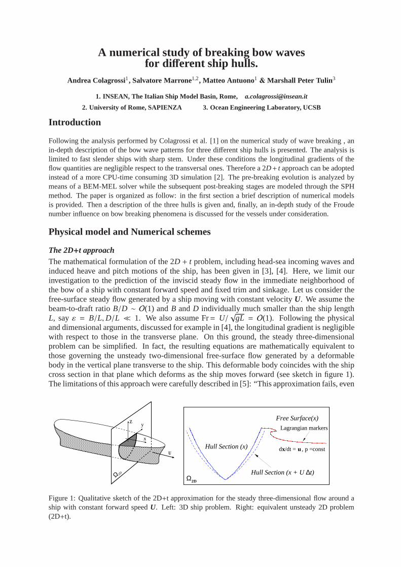
A numerical study of breaking bow wavesfor different ship hulls.

Andrea Colagrossi1, Salvatore Marrone1,2, Matteo Antuono1&Marshall Peter Tulin 3

1. INSEAN, The Italian Ship Model Basin, Rome, a.colagrossi@insean.it

2. University of Rome, SAPIENZA 3. Ocean Engineering Laboratory, UCSB

Introduction

Following the analysis performed by Colagrossi et al. [1] onthe numerical study of wave breaking , anin-depth description of the bow wave patterns for three different ship hulls is presented. The analysis islimited to fast slender ships with sharp stem. Under these conditions the longitudinal gradients of theflow quantities are negligible respect to the transversal ones. Therefore a 2D+ t approach can be adoptedinstead of a more CPU-time consuming 3D simulation [2]. The pre-breaking evolution is analyzed bymeans of a BEM-MEL solver while the subsequent post-breaking stages are modeled through the SPHmethod. The paper is organized as follow: in the first sectiona brief description of numerical modelsis provided. Then a description of the three hulls is given and, finally, an in-depth study of the Froudenumber influence on bow breaking phenomena is discussed for the vessels under consideration.

Physical model and Numerical schemes

The 2D+t approachThe mathematical formulation of the 2D + t problem, including head-sea incoming waves andinduced heave and pitch motions of the ship, has been given in[3], [4]. Here, we limit ourinvestigation to the prediction of the inviscid steady flow in the immediate neighborhood ofthe bow of a ship with constant forward speed and fixed trim andsinkage. Let us consider thefree-surface steady flow generated by a ship moving with constant velocityU. We assume thebeam-to-draft ratioB/D ∼ O(1) andB andD individually much smaller than the ship lengthL, sayε = B/L,D/L ≪ 1. We also assume Fr= U/

√gL = O(1). Following the physical

and dimensional arguments, discussed for example in [4], the longitudinal gradient is negligiblewith respect to those in the transverse plane. On this ground, the steady three-dimensionalproblem can be simplified. In fact, the resulting equations are mathematically equivalent tothose governing the unsteady two-dimensional free-surface flow generated by a deformablebody in the vertical plane transverse to the ship. This deformable body coincides with the shipcross section in that plane which deforms as the ship moves forward (see sketch in figure 1).The limitations of this approach were carefully described in [5]: “This approximation fails, even

U

xe

yeze

Ω 2D

zy

x

d /dt = , p =constx u

Free Surface(x)

Hull Section (x + U∆t)Ω2D

Hull Section (x)

Lagrangian markers

Figure 1: Qualitative sketch of the 2D+t approximation for the steady three-dimensional flow around aship with constant forward speedU. Left: 3D ship problem. Right: equivalent unsteady 2D problem(2D+t).

for slender bodies, in the vicinity of hull stagnation points and other corners, where the flow ishighly accelerated in the streamwise direction. The methodwould not apply, for example, toblunt bows, even for small (B/L). For fine bows, however, the stagnation point is weak, anddoes not exist on the free surface.”

The Mixed Eulerian–Lagrangian modelBefore breaking occurs, the flow is computed using the Mixed Eulerian-Lagrangian (MEL)method, as introduced independently by [6] and [7]. In the MEL method, the problem reducesto the following procedure:Step 1: given the velocity potentialϕ|FS on the free surface and the normal gradient∂ϕ/∂n|Bon the body boundary, a problem for the Laplace equation∇2ϕ = 0 can be set up and solvedand the velocity field∇ϕ can be computed everywhere in the fluid domain.Step 2: Using the well known Lagrangian form of the free-surface boundary conditions:

DϕDt=

12|∇ϕ|2 − gη

DrDt= ∇ϕ (1)

the evolution equations for the free-surface potential andfor the position of free-surface nodescan be stepped forward in time, providing, together with thebody boundary condition, a newset of boundary data for repeatingStep 1. In the present implementation, the solution ofthe mixed Dirichlet-Neumann problem for the Laplace equation is achieved numerically interms of Boundary Element Method. That is, the boundary of the domain is approximatedby a collection of rectilinear elements along whichϕ and∂ϕ/∂n are assumed to vary linearly.The relevant integrals are computed analytically and, after some manipulations, the discretizedintegral equations take the form of a system of linear algebraic equations

A

∂ϕ

∂n

∣

∣

∣

∣

∣

FS

ϕ|B

= B

ϕ|FS

∂ϕ

∂n

∣

∣

∣

∣

∣

B

, (2)

where the elements of the influence matricesA andB are only dependent on the geometry ofthe problem. The system is solved via a standard LU decomposition.The discretization of the free surface is controlled through numerical regridding and the gridrefinement is adapted to the evolution of the solution. More in detail collocation points may beadded in regions of high curvature. Regridding of the free surface is sometimes necessary tocontrol the size of the panel near the investigated intersection or to limit the number of pointson the free surface.

The SPH schemeIn the SPH method, the fluid domainΩ is discretized in a finite numberN of particlesrepresenting elementary fluid volumesdV, each one with its own local mass,dm, and otherphysical properties. In this context a generic fieldf at the positionr i of the i-th particle isapproximated through the convolution sum

〈 f 〉(r i) =∑

j

f j W(r i − r j; h) dVj (3)

where f j is the value of f associated to the generic particlej, dVj is its volume. FinallyW(r i − r j; h) is a kernel function whereh is a measure of its support and it is known in literatureassmoothing length. When it goes to zero the kernel functionW becomes a delta Dirac function.Note that the integration of the kernel function on its support is equal to one. For the ease ofnotation, hereinafter we denoteW(r i − r j; h) simply throughW(r j).

In practical SPH computations, the choice of the kernel function affects both the CPUrequirements and the stability properties of the algorithm. In this work a Gaussian kernel witha compact support has been adopted (see [8])The spatial derivatives of the fieldf can be estimated using the formula (3) obtaining:〈∇ f 〉(r i) =

∑

j (∇ f ) j W(r j) dVj. After some manipulation (for more details see [9]) it is possibleto move the gradient operator to the kernel and the previous formula can be approximated by

〈∇ f 〉(r i) =∑

j

f j ∇iW(r j)dVj − f (r i)∑

j

∇iW(r j)dVj (4)

where∇i denotes the derivative with respect tor i. One can note that this formula permits torecover exactly the null gradient of a constant function.The largest part of the SPH schemes is built on the assumptionthat the fluid is barotropic andweakly-compressible. The reference equations for the flow evolution are the classical Eulerequations. When the governing equations are written in the SPH contest, an artificial viscousterm is generally added inside the momentum equation for stability reasons (see for example[10]). Then, the discrete SPH scheme reads:

Dρi

Dt= −ρi

∑

j

(u j − ui) · ∇iW(r j) dV j ; pi = c20 (ρi − ρ0)

ρiDui

Dt= −∑

j

(p j + pi)∇iW(r j) dV j + ρi f i + α h c0 ρ0

∑

j

πi j ∇iW(r j) dV j

Dr i

Dt= ui

(5)

The symbolsρi, pi andui denote thei-th particle density, pressure and velocity,f is the bodyforce field,ρ0 is the density at the free surface andc0 is the sound velocity. The artificial viscoustermπi j is defined asπi j = (u j − ui) · r ji/|r i j |2 andr i j = −r ji = r i − r j. The parameterα controlthe magnitude of the artificial viscosity (in this workα = 0.01 has been used). The system (5)preserves the global mass and both the linear and angular momenta. Further forh going to zerothe system (5) recover the consistency with the Euler equations (seee.g[9]).

Ship technical specifications

In the present work we study the bow wave propagation for three different hulls: the DDG-51ARLEIGH BURKE-class, the NATO Research Vessel ALLIANCE andthe ATHENA researchvessel. The DDG-51 hull was designed for military purposes and has been widely studied forresearch aims at David Taylor Model Basin and at INSEAN (see for example the proceedingsof the “Workshop on CFD in Ship Hydrodynamics”, Gothenburg Sweden, September 2000).The ship length (L) is 142 m, the beam (B) at the waterline is 18 m, the draft (D) is equal to6.16 m and the displacement is equal to 8300 tons (speed about30 knots). For what concernsthe ALLIANCE vesselL=93 m, B=15.2 m,D=5.2 m and the displacement is equal to 2920tons (speed about 16 knots). Finally, for the ATHENA vesselL=47 m,B=6.9 m,D=1.5 m andthe displacement is equal to 209 tons (speed 13 knots on diesel, 35 knots on turbine). Figure2 shows the body plans for the three hulls under consideration. The DDG-51 vessel can beconsidered slender except for the bow bulb. The latter is notcrucial for the development of thedivergent wave but it limits the use of the 2D + t model. To overcome such a problem, in thenumerical simulation the volume of the bulb has been reduced. From a qualitative point of viewone can observe that the DDG-51 ship has the steepest stem profile and largest ratioB/D. Thelatter is quite similar to the ALLIANCE one which, on the contrary, shows the most gentle stemprofile. Finally the ATHENA hull has the largest ratioD/L and the smallest ratioB/D. As aconsequence of the differences above, different bow breaking patterns are expected.

Figure 2: Body plans of the DDG-51 (left panel), ALLIANCE (top-right panel) and ATHENA (bottom-right panel) hulls.

Discussion and conclusions

During the first stages of the evolution, the hull section moves toward the free surface similarlyto a water-entry phenomenon. Consequently, a violent waterdisplacement occurs generatinga water run-up along the ship bow. Such a motion is fed by the expansion of the ship crosssection leading to a bow breaking wave. This phenomenon is highlighted in the first threepanels of figure 3 where the breaking bow waves obtained through the BEM solver at differentFroude numbers and for the three hulls under consideration are shown. For what concerns theDDG-51 ship, the plunging jet becomes thicker and thicker asthe Froude number increases.Conversely, the plunging wave generated by the ATHENA ship keeps quite thin unless large

0 0.02 0.04 0.06 0.08 0.1

-0.04

-0.03

-0.02

-0.01

0

0.01

y/L

z/LFr =0.41

Fr =0.24

Fr =0.28

Fr =0.315Fr =0.35

0 0.02 0.04 0.06 0.08

-0.02

0

0.02

y/L

z/L

Fr =0.6416

Fr =0.30Fr =0.40

Fr =0.50

0 0.05 0.1 0.15

-0.06

-0.04

-0.02

0

0.02

y/L

z/LFr = 0.40

Fr = 0.25Fr = 0.30

Fr = 0.35

Figure 3: The bow breaking waves obtained through BEM simulations for the three hulls underconsideration: DDG-51 (top-left), ATHENA (top-right), ALLIANCE (bottom-left). The low-right panelshows a 3D view of the bow wave for the DDG-51 ship.

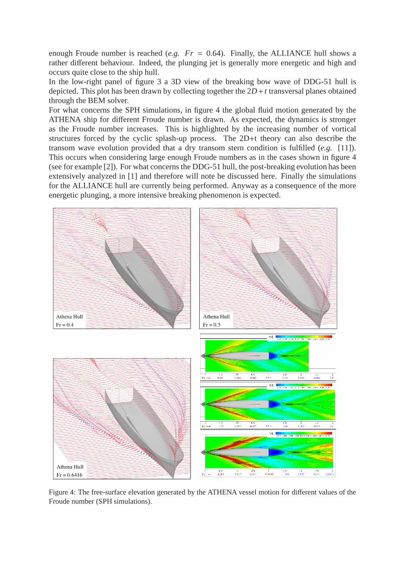
enough Froude number is reached (e.g. Fr = 0.64). Finally, the ALLIANCE hull shows arather different behaviour. Indeed, the plunging jet is generally moreenergetic and high andoccurs quite close to the ship hull.In the low-right panel of figure 3 a 3D view of the breaking bow wave of DDG-51 hull isdepicted. This plot has been drawn by collecting together the 2D+ t transversal planes obtainedthrough the BEM solver.For what concerns the SPH simulations, in figure 4 the global fluid motion generated by theATHENA ship for different Froude number is drawn. As expected, the dynamics is strongeras the Froude number increases. This is highlighted by the increasing number of vorticalstructures forced by the cyclic splash-up process. The 2D+t theory can also describe thetransom wave evolution provided that a dry transom stern condition is fulfilled (e.g. [11]).This occurs when considering large enough Froude numbers asin the cases shown in figure 4(see for example [2]). For what concerns the DDG-51 hull, thepost-breaking evolution has beenextensively analyzed in [1] and therefore will note be discussed here. Finally the simulationsfor the ALLIANCE hull are currently being performed. Anywayas a consequence of the moreenergetic plunging, a more intensive breaking phenomenon is expected.

Figure 4: The free-surface elevation generated by the ATHENA vessel motion for different values of theFroude number (SPH simulations).

AcknowledgementsThe present research activity is supported by Ministero Infrastrutture e Trasporti within theframeworks of the “Programma Ricerche INSEAN 2007-2009” and “Programma di Ricercasulla Sicurezza”.

References

[1] M. Landrini, A. Colagrossi and M.P. Tulin,Numerical Studies of Wave Breaking Comparedto Experimental Observations, In Proc. of 4th Numerical Towing Tank Symposium (Ed. V.Bertram), Hamburg, 2001.

[2] A. Colagrossi, M. Antuono and S. Marrone,A 2D+t SPH model with enhanced solidboundary treatment, Proc. of 4th International SPHERIC Workshop, Nantes, France, May2009.

[3] H. Maruo and W. Song,Nonlinear Analysis of Bow Wave Breaking and Deck Wetnessof a High-Speed Ship by the Parabolic Approximation, 20th Symposium on NavalHydrodynamics, University of California, Santa Barbara.,1994.

[4] M. Wu, M.P. Tulin and E. Fontaine,On the Simulation of Amplified Bow Waves Induced byMotion in Head Seas, J. Ship Res., 2003.

[5] M.P. Tulin and M. Wu, Divergent bow waves, Proc. of the 21st ONR Symp. on NavalHydrodynamics, Trondheim, Norway, National Academy Press, Wash. D.C., pp. 99–117,(1996).

[6] M.S. Longuet-Higgins & E.D. Cokelet,the deformation of steep surface waves on water. I.A numerical method of computation., Proc. of the Roy. Soc. Lond. A. 350, (1976).

[7] O.M. Faltinsen,Numerical solutions of transient nonlinear freeÂŋsurface motion outsideor inside moving bodies, Proc. of the Second International Conference on NumericalShipHydrodynamics, University of California, Berkeley, September (1977).

[8] Landrini M., Colagrossi A., Greco M., Tulin M.P., “Gridless simulations of splashingprocesses and near-shore bore propagation”,Journal of Fluid Mechanics, 591, 183–213(2007).

[9] Colagrossi A., Antuono M., Le Touzé D., “Theoretical considerations on the free surfacerole in the SPH model”,Phys. Rev. E., 79/5: 056701:1–13 (2009)

[10] J.J. Monaghan,Smoothed Particle Hydrodynamics, Reports on Progress in Physics,Institute of Physics Publishing,68, 1703-1759, (2005).

[11] C. Lugni, A. Colagrossi, M. Landrini and O.M. Faltinsen, Experimental and NumericalStudy of Semi-displacement Mono-hull and Catamaran in calmwater and incident waves,Proc. of 25th Symp.on Naval Hydrodynamics, St. John’s, Canada, August 2004.

Numerical investigation of the scouring around pipelines

Giuseppina Colicchio1, Matteo Mattioli2, Claudio Lugni1, Maurizio Brocchini2

1- INSEAN, Rome/Italy. g.colicchio@insean.it2- Universita Politecnica delle Marche - Italy

1 Introduction

Pipelines laid on the seabed interact with currents and waves, generating a local velocity fieldand pressure gradients between the upstream and downstream sides of the pipe. If the pipeis laid on a sandy bottom, the interaction of pressure gradients with the bottom can drive aseepage flow, allowing the wet sand to be dragged by the shear stress. In some cases this effectcan be particularly large, washing away the sand beneath the pipeline and giving rise to somescouring underneath the pipe itself.

The investigation of the evolution of the pipe/seabed configuration has a large relevance forpipeline design because a free-span occurrence and persistence may cause the vibration of thepipeline and the accumulation of unacceptable fatigue damages. Therefore, for a reliable ap-proach to pipeline design, the possibility of accurately predicting both generation and evolutionof scour-induced free-spans during the first years of pipe laying has a large relevance.

A review of the work on the local sour below pipelines can be found in [1-3].

The majority of the studies available in the literature are based on experiments. This led toa fundamental understanding and to the physical modeling of the phenomenon. Nonetheless,numerical modeling is necessary during the design stage. The first numerical algorithms werebased on the potential flow theory [4], even though such a theory is not able to represent thevorticity generated downstream of the body of interest, the results were encouraging because thefront deformation was successfully predicted. Later on, full Navies-Stokes solver with turbulencemodels and sediment transport equations [5-7] were introduced. The main limits of thesealgorithms is in the capturing of the inception of the scouring. The use of a boundary-fittedmesh either leads to the use of: either (1) an initial infinitesimal gap between the cylinder andthe sandy bottom or (2) two simulations [one with the pipeline (i.e. cylinder) touching thebottom and, after a threshold value, to a new topology where a gap between the body andthe bottom is applied]. In both cases the time of inception of the free-span depends on thesimulation parameters. Here a new treatment of the boundary of the computational domainenables the capturing of the topological change in the domain, making the prediction of thestart of the free-span more reliable.

2 Numerical Model

A Navier-Stokes solver is coupled with a model of the granular sand layer. No turbulence modelis introduced, because a stretching of the mesh is used and the mesh size close to the bottomenable a DNS-type computation.

As described in figure 1, the computational domain is divided into three parts according to thephysical features of the local flow: 1) a pure-water domain, 2) a solid domain with consolidatedsand and 3) a water-sand mixture, lying in between, where sand is trapped into the waterbecause of the friction induced by the water.

The fluid regions (1) and (3) are modeled as a single-fluid domain with variable properties of

PureWater

Water−Sand Mixture

Sand

Figure 1: The definition of the three computational domains.

mass and viscosity and are governed by the mass-conservation and Navier-Stokes equations:

Dρ

Dt= 0

ρDu

Dt= −∇p + ∇(µD) + g

(1)

discretized on a Cartesian mesh and solved with second-order finite-difference schemes and anapproximate projection method for the pressure. The fluid properties ρ and µ are defined as aweighted average between the density and viscosity of water and of the muddy flow as:

ρ = ρwater(1 − c) + ρsandcµ = µwater(1 − c) + µsandc

(2)

where c is the local concentration of sand, assuming that c = 1 on the bottom and c = 0 in thepure water. Substituting the first equation of (2) in the first equations of (1), one obtains thecontinuity equation for the sand concentration c

∂c

∂t+ u · ∇c = 0. (3)

This equation is corrected to become

∂c

∂t+ ∇(c(u + ud)) = 0 (4)

where ud is the limit velocity of the single sand grain, determined as the limit velocity of anequivalent radius sphere moving in a domain with equivalent pressure gradients ud = ∇p/ρ [8].The velocity is set equal to zero on the compact-sand boundary. This formulation allows thesand to pile up on the compact bottom and takes into account the fact that sand is composedof single grains that would fall on the bottom in rest conditions.

The boundary of the fluid domain, the second zone of the model, is represented on a Cartesiangrid using a level-set function φ. It represents a signed distance function either from the compactsand or the cylinder. At these boundaries the fluid velocity satisfies the following equation:

u = s(φ)ufluid + (1 − s(φ))uboundary (5)

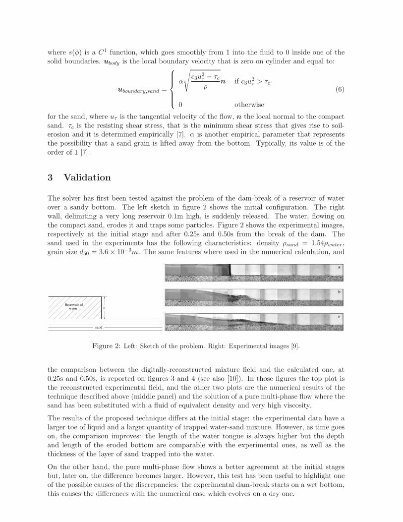
where s(φ) is a C1 function, which goes smoothly from 1 into the fluid to 0 inside one of thesolid boundaries. ubody is the local boundary velocity that is zero on cylinder and equal to:

uboundary,sand =

α

√

c3u2τ − τc

ρn if c3u

2τ > τc

0 otherwise

(6)

for the sand, where uτ is the tangential velocity of the flow, n the local normal to the compactsand. τc is the resisting shear stress, that is the minimum shear stress that gives rise to soil-erosion and it is determined empirically [7]. α is another empirical parameter that representsthe possibility that a sand grain is lifted away from the bottom. Typically, its value is of theorder of 1 [7].

3 Validation

The solver has first been tested against the problem of the dam-break of a reservoir of waterover a sandy bottom. The left sketch in figure 2 shows the initial configuration. The rightwall, delimiting a very long reservoir 0.1m high, is suddenly released. The water, flowing onthe compact sand, erodes it and traps some particles. Figure 2 shows the experimental images,respectively at the initial stage and after 0.25s and 0.50s from the break of the dam. Thesand used in the experiments has the following characteristics: density ρsand = 1.54ρwater ,grain size d50 = 3.6 × 10−3m. The same features where used in the numerical calculation, and

sand

hReservoir of water

Figure 2: Left: Sketch of the problem. Right: Experimental images [9].

the comparison between the digitally-reconstructed mixture field and the calculated one, at0.25s and 0.50s, is reported on figures 3 and 4 (see also [10]). In those figures the top plot isthe reconstructed experimental field, and the other two plots are the numerical results of thetechnique described above (middle panel) and the solution of a pure multi-phase flow where thesand has been substituted with a fluid of equivalent density and very high viscosity.

The results of the proposed technique differs at the initial stage: the experimental data have alarger toe of liquid and a larger quantity of trapped water-sand mixture. However, as time goeson, the comparison improves: the length of the water tongue is always higher but the depthand length of the eroded bottom are comparable with the experimental ones, as well as thethickness of the layer of sand trapped into the water.

On the other hand, the pure multi-phase flow shows a better agreement at the initial stagesbut, later on, the difference becomes larger. However, this test has been useful to highlight oneof the possible causes of the discrepancies: the experimental dam-break starts on a wet bottom,this causes the differences with the numerical case which evolves on a dry one.

Figure 3: Comparison between the experimental reconstruction of the field [9] (top panel) and numericaldata at t=0.25s obtained with two different techniques (adapted from [10]).

Figure 4: Comparison between the experimental reconstruction of the field [9] (top panel) and numericaldata at t=0.50s obtained with two different techniques (adapted from [10]).

4 Preliminary results

Finally, the numerical scheme was applied to a preliminary study of more realistic problem likethat described in figure 5. There the physical parameters of interests are described. A cylinder,

H

D

ε

U

h

L

Figure 5: Sketch of the problem of a cylinder semi-detached from the bottom in a steady current.

of diameter D = 0.1m, is placed 0.35m below the free-surface and at a distance of ǫ = 0.005mfrom the initial compact bottom. A constant incoming current of strength U = 0.2m/s causesthe deformation of the compact-sand bottom. The characteristics of the sand used in thecomputation are the following: density ρsand = 1.54ρwater , θc = 0.048, d50 = 3.6 × 10−4m. Theused computational domain has a lenght L = 10D and a height H = 5.5D with the centre ofthe cylinder placed 0.3D downstream of the inlet boundary (see figure 5).

The solver is able to model the problem illustrated in the figure but, to get a computationallyfast answer, the numerical model has been simplified. The upper boundary has been madecoincident with the undisturbed free surface, and a constant pressure has been applied asboundary condition in that region, practically, the problem has been linearized around the freesurface.

Moreover, the parameter α appearing in equation (6) has been chosen equal to 35, to accelleratethe erosion of the sand.

The results of such a technique are shown in figure 6. Well evident is, beyond the vortexshedding at the lee side of the cylinder, the bottom erosion on the upstream side of the bodyand the consequent sand deposition downstream of the cylinder.

0.2 0.4 0.6 0.8 1

0

0.1

0.2

0.3

0.2 0.4 0.6 0.8 1

0

0.1

0.2

0.3

0.2 0.4 0.6 0.8 1

0

0.1

0.2

0.3

0.2 0.4 0.6 0.8 1

0

0.1

0.2

0.3

0.2 0.4 0.6 0.8 1

0

0.1

0.2

0.3

0.2 0.4 0.6 0.8 1

0

0.1

0.2

0.3

Figure 6: Erosion of the bottom below the cylinder at a time interval of 1s.

5 Conclusions and future work

The use of a Level Set description of a body in a flow field allows the application of the Navies-Stokes solver to the study of the problem of pipe-soil interaction. A parameterized velocityof erosion is used to calculate the deforming boundary of the fluid domain and the quantityof sand dispersed into the water. Then the fluid mixture is computed as a fluid domain withdensity variable as function of the sand concentration.

A first validation of the solver has been shown here, the analysis of the results compared withexperimental data for a pipe in current [8] is underway. Such an analysis is time consumingbecause it involves the study of the parameters that have been introduced above, however someresults of this effort will be shown at the workshop.

References

[1] Sumer, B. M., and Fredsoe, J. (1992). A review of wave/current-induced scour around pipelines.Chapter 217, Proc., 23rd Int. Conf. on Coast. Engrg., ASCE, New York, Vol. 3, 2839-2852.

[2] Sumer, B. M., and Fredsoe, J. (1999). Wave scour around structures. Advances in coastal and oceanengineering, Philip L.-F. Liu, ed., Vol. 4, 191-249.

[3] Whitehouse, R. J. S. (1998). Scour at marine structures, Thomas Telford, London.

[4] Hansen, E. A., Fredsc, J., and Ye, M. (1986). Two-dimensional scour below pipelines. Proc., 5th Int.Symp. on Offshore Mech. and Arctic Engrg., ASME, New York, 670-678.

[5] Leeuwestein, W., Bijker, E. A., Peerbolte, E. B., and Wind, H. G. (1985). The natural selfburial ofsubmarine pipelines. Proc., 4th Int. Conf. on Behaviour of Offshore Struct. (BOSS), Elsevier Science,Amsterdam, 717-728.

[6] Li, F., and Cheng, L., (2001) Prediction of Lee-wake scouring of pipelines in currents, J. Wtrwy.,Port, Coast. and Oc. Engrg., ASCE, 127(2), 106111.

[7] Smith, H. D., and Foster, D. L., (2002) Modelling of Flow and Scour Around a Pipeline, Proc. Coast.Eng. 2002, 1722-1732.

[8] Mao, Y. (1986). The Interaction Between a Pipeline and an Erodible Bed. PhD thesis, Technical

University of Denmark.

[9] Fraccarollo, L., Capart, H., (2002). Riemann wave description of erosional dam-break flows.J. Fluid Mech., 461, 183-228.

[10] Colicchio, G., Colagrossi, A., Brocchini, M., Venturi, M., Drago, M., (2007). Pipe-soilinteraction: an evaluation of a numerical model, 26th OMAE,Sand Diego, USA.

Correlation of bow and stern slamming occurrence with whipping excitation for a cruise vessel

Daniele Dessi and Michele De Luca

d.dessi@insean.it

INSEAN - Italy

Introduction

In this paper, the correlation between the bow and stern slamming impacts with the bending moment response of a cruise ship is investigated via segmented model tests based on the elastic backbone technique. The tests, performed at the Italian ship model basin, concerned both head and following wave conditions, in order to compare the relative importance of the two phenomena. In particular, stern slamming has recently revealed to be a serious drawback for the passenger comfort of certain cruise ships during approach to harbors and it still needs further investigation to provide reliable data for comparison with CFD predictions. The detection of slamming impacts is based on the analysis of the local draught obtained from the measurements of the wave probes placed on-board. These probes, after precise calibration and proper signal processing, allowed to count the slamming occurrences with sufficient accuracy. The critical conditions for the slamming occurrence were determined, highlighting the dependence of the number of slamming events on the ship speed, the significant wave height and the wave period. A particular attention was devoted to the correlation of the level of excitation, represented by the time averaged whipping response expressed in terms of the vertical bending moment, with the number of slamming events.

Experimental Setup

A segmented model of the cruise ship was constructed accordingly to the backbone-modeling technique (Dessi and Mariani, 2008). The ship length between perpendiculars is about 290 m at full-scale, and in Fig. 1 the shape of the hull sections can be appreciated. In order to scale the ship bending behaviour, the bending stiffness and shear area distributions, obtained by collapsing the structural 3D FE model of the full-scale ship into an equivalent Timoshenko beam, were used as reference data. The model scale was set to 1 : 60, that implies accordingly to the Froude scaling law a model frequency of the two-node bending mode in air close to 10.1 Hz. This value was assumed as the target value for the design of the backbone of the scaled model, since there was no way to take into account closely the higher-order modes due to the large value of the reference shear deformability (if compared, for instance, with that of other ships). The elastic beam was made of an aluminum alloy with 6 elements of different length and transverse section, accordingly to the reference distribution of the sectional moment of inertia. From the vibration tests in water, it was observed that the two-node mode vibrated at about 7.4 Hz, a value close to the reference value. The hull was divided into 5 segments, each one connected to the elastic beam with a vertical steel leg. The longitudinal positions of the hull cuts were chosen in order to restrict the bow and the stern segment to the hull portions where slamming was present both in head and following sea. These segments were made of fiberglass, whereas the gaps between adjacent segments are made water-tight by using rubber straps. The segments were numbered from the bow (No 1) to the stern (No 5), as shown in Fig. 1. As a rigid-body, the physical model was free to heave, to pitch and, partially, to surge. In every test the following physical quantities were measured: (i) the absolute wave height in two locations, (ii) the rigid-body degrees of freedom (dofs), (iii) the vertical bending moment on several beam sections and (iv) the relative wave elevation at several sections. The incoming, absolute wave height was measured by using two finger probes placed at fixed positions with respect to the towing tank. The heave, pitch and surge dofs were measured with the Krypton Rodymm DMM

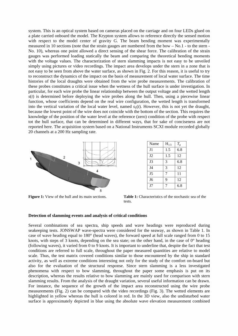
system. This is an optical system based on cameras placed on the carriage and on four LEDs glued on a plate carried onboard the model. The Krypton system allows to reference directly the sensed motion with respect to the model center of gravity G. The beam bending moment was experimentally measured in 10 sections (note that the strain gauges are numbered from the bow – No.1 - to the stern - No. 10), whereas one point allowed a direct sensing of the shear force. The calibration of the strain gauges was performed loading statically the beam and comparing the theoretical bending moments with the voltage values. The characterization of stern slamming impacts is not easy to be unveiled simply using pictures or video recordings. The impact area develops under the stern in a zone that is not easy to be seen from above the water surface, as shown in Fig. 2. For this reason, it is useful to try to reconstruct the dynamics of the impact on the basis of measurement of local water surface. The time histories of the local draughts were obtained from the wire probe measurements. The calibration of these probes constitutes a critical issue when the wetness of the hull surface is under investigation. In particular, for each wire probe the linear relationship between the output voltage and the wetted length s(t) is determined before deploying the wire probes along the hull. Then, using a piecewise linear function, whose coefficients depend on the real wire configuration, the wetted length is transformed into the vertical variation of the local water level, named sZ(t). However, this is not yet the draught, because the lowest point of the wire does not coincide with the bottom of the section. This requires the knowledge of the position of the water level at the reference (zero) condition of the probe with respect tot the hull surface, that can be determined in different ways, that for sake of conciseness are not reported here. The acquisition system based on a National Instruments SCXI module recorded globally 20 channels at a 200 Hz sampling rate.

Name H1/3 Tp

J1 1.5 6.8 J2 1.5 12 J3 3 6.8 J4 3 12 J5 7 11 J6 9 12 J7 7 6.8

Figure 1: View of the hull and its main sections. Table 1: Characteristics of the stochastic sea of the tests.

Detection of slamming events and analysis of critical conditions

Several combinations of sea spectra, ship speeds and wave headings were reproduced during seakeeping tests. JONSWAP wave-spectra were considered for the seaway, as shown in Table 1. In case of wave heading equal to 180° (head waves), the forward speed at full scale ranged from 0 to 15 knots, with steps of 3 knots, depending on the sea state; on the other hand, in the case of 0° heading (following waves), it varied from 0 to 9 knots. It is important to underline that, despite the fact that test conditions are referred to full scale, throughout the paper measured quantities are relative to model scale. Thus, the test matrix covered conditions similar to those encountered by the ship in standard activity, as well as extreme conditions interesting not only for the study of the comfort on-board but also for the evaluation of the structural response. Since stern slamming is a less investigated phenomena with respect to bow slamming, throughout the paper some emphasis is put on its description, whereas the results relative to bow slamming are mainly used for comparison with stern slamming results. From the analysis of the draught variation, several useful information can be drawn. For instance, the sequence of the growth of the impact area reconstructed using the wire probe measurements (Fig. 2) can be compared with the video recordings (Fig. 3). The wetted elements are highlighted in yellow whereas the hull is colored in red. In the 3D view, also the undisturbed water surface is approximately depicted in blue using the absolute wave elevation measurement combined

with the rigid-body motion. The signal was then translated using an averaged phase velocity depending on the sea characteristics just to give an idea of the undisturbed wave surfaces. After that the time histories of the draughts d(t) have been determined, it is necessary to obtain the derivative of the draught with respect to time, . Due to the lack of smoothness of the wire probe signals, it is necessary to filter the signal in order to eliminate high frequency fluctuations. In fact, these fluctuations, though small in amplitude, may determine unphysical spikes in the time derivative of the draughts.

)(td&

Following Ochi and Motter (1973) the necessary and sufficient conditions for the occurrence of a slamming event are that i) the relative motion between ship and waves must be equal to the sectional draft and ii) the relative velocity is equal or greater to a threshold velocity vL at the time the bow hull touches the water surface. The above conditions were originally issued considering only the possibility of bottom slamming. In the case of bow slamming in head waves, the sectional draft at a certain station, used to discriminate the hull emersion, is a well defined geometrical quantity that does not require any additional discussion. For fast ships, it is usually possible to use the experimental time histories of the absolute wave elevation and of the rigid body motions to derive the relative displacement (or the undisturbed relative wave elevation) to be used as the key variable to discriminate the wetness of the surface.

Figure 2: Reconstruction of the wetted area during an impact sequence.

Figure 3: Sequence of the stern slamming on the afterbody for sea condition (Vship = 0).

However, in the case of slow forward speed regimes, as well as in the case of stern slamming, the wave surface impacting on the stern in following waves is affected by the presence of the hull and the use of the undisturbed wave elevation gives just an approximate picture of the real situation. If the local draught sensors can provide the correct information to estimate the relative position between the hull bottom and the water surface, it is also worth to note that in the case of stern slamming we were however interested to an equivalent wetness of the rear hull bottom. In fact, since the wetness of the flat stern is more relevant than that of the keel, the complex stern section has been replaced by an equivalent plane (the trace on the x-z plane is depicted in green in Fig. 4). This allows to give an unique threshold for the local draught to determine the significant wetness of each section. Another critical aspect is provided by the choice of threshold for the relative velocity, that is depending on what has to be considered as slamming. A quite general rule was proposed by Ochi and Motter (1973) based on full scale trial observations for different ships and sea states; according to the experimental results the critical condition is given, if a probability model for slamming pressure is assumed, in term of the probability of a slam impact reaching a level of 0.03 and/or in term of the significant amplitude of the acceleration at the bow greater than 0.4g. These values refer to a condition in which slam occurs but are not able to produce damage. Moreover Ferro and Mansour (1985), on the basis of the above considerations, summarized the Ochi and Motter condition in the following simple formula:

ppL L29.0v = where Lpp is the ship length at waterline. The actual thresholds that are used in this

work derive from a previous analysis that was carried out by Dessi et al. (2007), that correlated the water entry velocity with the presence of evident whipping.

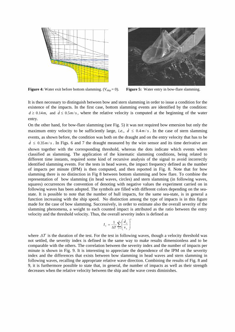
Figure 4: Water exit before bottom slamming. (Vship = 0). Figure 5: Water entry in bow-flare slamming.

It is then necessary to distinguish between bow and stern slamming in order to issue a condition for the existence of the impacts. In the first case, bottom slamming events are identified by the condition:

, where the relative velocity is computed at the beginning of the water entry.

smdmd /5.0and,14.0 ≤≥ &

On the other hand, for bow-flare slamming (see Fig. 5) it was not required bow emersion but only the maximum entry velocity to be sufficiently large, i.e., . In the case of stern slamming events, as shown before, the condition was both on the draught and on the entry velocity that has to be

. In Figs. 6 and 7 the draught measured by the wire sensor and its time derivative are shown together with the corresponding threshold, whereas the dots indicate which events where classified as slamming. The application of the kinematic slamming conditions, being related to different time instants, required some kind of recursive analysis of the signal to avoid incorrectly identified slamming events. For the tests in head waves, the impact frequency defined as the number of impacts per minute (IPM) is then computed, and then reported in Fig. 8. Note that for bow slamming there is no distinction in Fig 8 between bottom slamming and bow flare. To combine the representation of bow slamming (in head waves, circles) and stern slamming (in following waves, squares) occurrences the convention of denoting with negative values the experiment carried on in following waves has been adopted. The symbols are filled with different colors depending on the sea-state. It is possible to note that the number of hull impacts, for the same sea-state, is in general a function increasing with the ship speed. No distinction among the type of impacts is in this figure made for the case of bow slamming. Successively, in order to estimate also the overall severity of the slamming phenomena, a weight to each counted impact is attributed as the ratio between the entry velocity and the threshold velocity. Thus, the overall severity index is defined as

smd /4.0≤&

smd /35.0≤&

∑= ⎟

⎟⎠

⎞⎜⎜⎝

⎛

Δ=

N

j L

rjS

dT

I1

2

v1 &

where ΔΤ is the duration of the test. For the test in following waves, though a velocity threshold was not settled, the severity index is defined in the same way to make results dimensionless and to be comparable with the others. The correlation between the severity index and the number of impacts per minute is shown in Fig. 9. It is interesting to appreciate the dependence of the IPM on the severity index and the differences that exists between bow slamming in head waves and stern slamming in following waves, recalling the appropriate relative wave direction. Combining the results of Fig. 8 and 9, it is furthermore possible to state that, in general, the number of impacts as well as their strength decreases when the relative velocity between the ship and the wave crests diminishes.

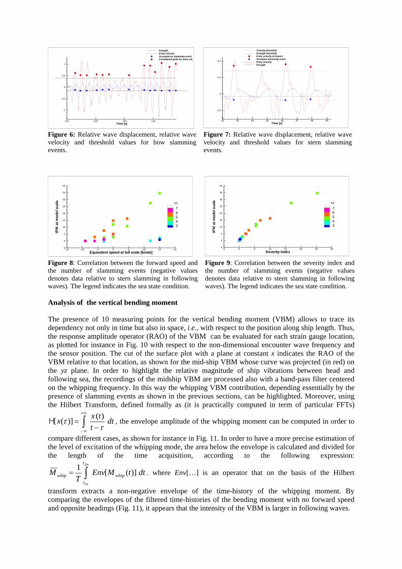
Time [s]115 120 125 130

-1

-0.5

0

0.5

1

DraughtEntry velocityAccepted as slamming eventConsidered peak for entry vel.

Time [s]42 43 44 45 46 47 48 49

-0.2

0

0.2

0.4

Velocity thresholdDraught thresholdEntry velocity at impactAccepted slamming eventEntry velocityDraught

Figure 6: Relative wave displacement, relative wave velocity and threshold values for bow slamming events.

Figure 7: Relative wave displacement, relative wave velocity and threshold values for stern slamming events.

Equivalent speed at full scale [knots]

IPM

atm

odel

scal

e

-15 -10 -5 0 5 10 15 20-5

0

5

10

15

20

25

30

35

40

SS

76543

Severity Index

IPM

atm

odel

scal

e

-5 0 5 10 15 20 25 30-5

0

5

10

15

20

25

30

35

40

SS

76543

Figure 8: Correlation between the forward speed and the number of slamming events (negative values denotes data relative to stern slamming in following waves). The legend indicates the sea state condition.

Figure 9: Correlation between the severity index and the number of slamming events (negative values denotes data relative to stern slamming in following waves). The legend indicates the sea state condition.

Analysis of the vertical bending moment

The presence of 10 measuring points for the vertical bending moment (VBM) allows to trace its dependency not only in time but also in space, i.e., with respect to the position along ship length. Thus, the response amplitude operator (RAO) of the VBM can be evaluated for each strain gauge location, as plotted for instance in Fig. 10 with respect to the non-dimensional encounter wave frequency and the sensor position. The cut of the surface plot with a plane at constant x indicates the RAO of the VBM relative to that location, as shown for the mid-ship VBM whose curve was projected (in red) on the yz plane. In order to highlight the relative magnitude of ship vibrations between head and following sea, the recordings of the midship VBM are processed also with a band-pass filter centered on the whipping frequency. In this way the whipping VBM contribution, depending essentially by the presence of slamming events as shown in the previous sections, can be highlighted. Moreover, using the Hilbert Transform, defined formally as (it is practically computed in term of particular FFTs)

∫+∞

∞− −= dt

ttxxτ

τ )()]([Η , the envelope amplitude of the whipping moment can be computed in order to

compare different cases, as shown for instance in Fig. 11. In order to have a more precise estimation of the level of excitation of the whipping mode, the area below the envelope is calculated and divided for the length of the time acquisition, according to the following expression:

∫=init

whipwhip dttMEnvT

M )]([fint

1. where Env[…] is an operator that on the basis of the Hilbert

transform extracts a non-negative envelope of the time-history of the whipping moment. By comparing the envelopes of the filtered time-histories of the bending moment with no forward speed and opposite headings (Fig. 11), it appears that the intensity of the VBM is larger in following waves.

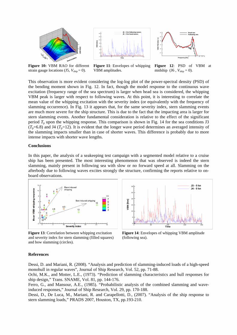
Time

VB

M[N

m]

0 50 100 150 2000

20

40

60

80

100

120

140J6 - 0 kn following wavesJ6 - 0 kn head waves

Frequency [Hz]

VB

MP

SD

[Nm

/s]

5 10 15 20 25

10-1

100

101

102

103

104 Head seaFollowing sea

Figure 10: VBM RAO for different strain gauge locations (J5, Vship = 0).

Figure 11: Envelopes of whipping VBM amplitudes.

Figure 12: PSD of VBM at midship (J6 , Vship = 0).

This observation is more evident considering the log-log plot of the power-spectral density (PSD) of the bending moment shown in Fig. 12. In fact, though the model response to the continuous wave excitation (frequency range of the sea spectrum) is larger when head sea is considered, the whipping VBM peak is larger with respect to following waves. At this point, it is interesting to correlate the mean value of the whipping excitation with the severity index (or equivalently with the frequency of slamming occurrence). In Fig. 13 it appears that, for the same severity index, stern slamming events are much more severe for the ship structure. This is due to the fact that the impacting area is larger for stern slamming events. Another fundamental consideration is relative to the effect of the significant period Tp upon the whipping response. This comparison is shown in Fig. 14 for the sea conditions J3 (Tp=6.8) and J4 (Tp=12). It is evident that the longer wave period determines an averaged intensity of the slamming impacts smaller than in case of shorter waves. This difference is probably due to more intense impacts with shorter wave lengths.

Conclusions

In this paper, the analysis of a seakeeping test campaign with a segmented model relative to a cruise ship has been presented. The most interesting phenomenon that was observed is indeed the stern slamming, mainly present in following sea with slow or no forward speed at all. Slamming on the afterbody due to following waves excites strongly the structure, confirming the reports relative to on-board observations.

VB

M[N

m]

0

Time0 50 100 150 200

5

10

15

20

25

30 J3 - 0 knJ4 - 0 kn

Figure 13: Correlation between whipping excitation and severity index for stern slamming (filled squares) and bow slamming (circles).

Figure 14: Envelopes of whipping VBM amplitude (following sea).

References Dessi, D. and Mariani, R. (2008). “Analysis and prediction of slamming-induced loads of a high-speed monohull in regular waves”, Journal of Ship Research, Vol. 52, pp. 71-88. Ochi, M.K., and Motter, L.E., (1973). “Prediction of slamming characteristics and hull responses for ship design,” Trans. SNAME, Vol. 81, pp. 144-176. Ferro, G., and Mansour, A.E., (1985). “Probabilistic analysis of the combined slamming and wave-induced responses,” Journal of Ship Research, Vol. 29, pp. 170-188. Dessi, D., De Luca, M., Mariani, R. and Carapellotti, D., (2007). “Analysis of the ship response to stern slamming loads,” PRADS 2007, Houston, TX, pp.193-210.

1

LES OF THE FLOW AROUND AN OSCILLATING CYLINDER

Andreas Feymark‡, Niklas Alin†,‡, Rickard Bensow‡ & Christer Fureby†,‡ ‡Dept. of Shipping and Marine Technology, Chalmers University of Technology,

SE-412 96, Göteborg, Sweden †Defense Security Systems Technology, The Swedish Defense Research Agency – FOI,

SE 147 25 Tumba, Stockholm, Sweden andreas.feymark@chalmers.se

Viscous flow over an oscillating circular cylinder continues to attract much attention in both the academic and practical engineering arenas due to the rich blend of physics included. This non-linear flow, arising from the in-teraction of the fluid and the structure, is largely influenced by the combination of the oscillating amplitude ratio A/D and the excitation frequency ratio

€

fe / f0. At the right combination, the flow may induce one or more fasci-nating and complex phenomena such as hysteresis, bifurcation, synchronization and transformation or competi-tion of the vortex shedding patterns. These pose a great challenge to both theoretical and experimental tech-niques. Experimental studies of longitudinally forced cylinder oscillations are relatively less common compared to transversely forced excitations. Perhaps this is because the longitudinal fluctuating force Fx exerted on the cylinder is weaker, being only about one tenth in magnitude of the transverse fluctuating force Fy [1]. Nonethe-less, in hydrodynamic flows, this Fx component has been known to excite braced members of offshore struc-tures, marine piles and submarine periscopes [2], and is of engineering significance. Due to the significant achievements in scientific computing during the last two decades flow problems of engineering interest can now be studied, see e.g. [3] and references therein, using Large Eddy Simulation (LES), [4-5], and Detached Eddy Simulation (DES), [6]. The use of LES and DES enable us to predict not only the mean flow but also the transient nature of the flow that is not accessible by conventional Reynolds Averaged Navier-Stokes (RANS) models, [7]. As most structures are not perfectly rigid, fluid structure interactions may be important in some cases as already mentioned. For such problems, the unsteady coupling between the turbu-lent flow and the structure will require unsteady simulation models such as DES or LES, and in the current study we combine the aims of improving the understanding of the flow past an oscillatory cylinder and to de-velop a framework for fluid structure interactions using LES. Fixed and oscillating cylinders have previously been studied, both experimentally, [8-12], and numeri-cally, [13-15]. This study is an extension of the previous work of Liefvendahl & Lillberg, [13], and aims at fur-ther improving our understanding of this flow and aid in the validation of an LES-based fluid structure interac-tion methodology for complex engineering problems. The main contributions of the present study is to examine the grid resolution requirements, the power spectrum of the forces, the interdependence of the axial and lateral forces, the requirements for subgrid wall-models and to further improve our current understanding of the flow physics and how the forces acting on the cylinder are generated. The data of Cetiner & Rockwell, [10,12], is used for validation. In their set-up, a circular cylinder with diameter D=0.0254 m and length of L=0.0318 m, was placed in a custom designed water tunnel with a depth of 0.610 m, a width of 0.914 m, and a length of 4.93 m. The cylinder was mounted in a horizontal, cantilevered arrangement at a location halfway between the free surface and the bottom of the channel. The flow is characterized by the frequency ratio

€

fe / f0 between the fre-quency of the cylinder,

€

fe, and the von-Kármán shedding frequency,

€

f0 , and the velocity ratio

€

U/2πfeA betwe-en the free-stream velocity, U, and the maximum velocity of the cylinder,

€

2πfeA . In the experiments, the Keulegan-Carpenter number,

€

KC=2πA/D , and the frequency of the streamwise motion of the cylinder was kept constant at

€

KC=6 and

€

fe=0.28Hz respectively, where as the Re number was varied between 405 and 2482. Then, for fixed ratios of

€

fe / f0 and

€

U/2πfeA , using a Strouhal number definition of

€

St= f0D/U=0.2 , the parame-ters U, A, and

€

f0 may be estimated. The same approach is used for the simulations carried out. Figure 1a pre-sents a schematic of the computational configuration including dimensions and boundary conditions. The base-line grid contains approximately 1.25 Mcells distributed as in figure 1b, where also some key flow features are

2

presented in terms of iso-surfaces of the second invariant of the velocity gradient tensor. In the on going study results from several cases will be considered to examine how well the computational model can capture the range of observed phenomena, [8-12], resulting in very different flow features depending on the choice of pa-rameters, and how different computational parameters such as grid resolution and subgrid modeling affects the results. As an illustration we present in Figure 1b the case for which

€

fe / f0=1 and

€

U/2πfeA=0.83, in other words an oscillation at the von Kármán frequency.

(a) (b)

Figure 1. (a) Schematic of the computational domain and boundary conditions and (b) grid and vorticity dis-tribution in terms of the second invariant of the velocity gradient tensor, Note the grid deformation in (b).

LES, [2-3], is based on the idea of separating scales, and splitting the flow into two regimes by which all scales larger than the characteristic grid spacing, ∆, are resolved using a space/time accurate algorithm and only the effects of the unresolved subgrid scales on the large resolved scales are modeled. The direct computation of the large energy containing eddies (being flow and geometry dependent) gives LES, [16], although at a higher computational cost, more generality than RANS, in which the turbulence is treated statistically. Far from walls, the details of the subgrid models are of less importance, as long as it provides sufficient dissipation to emulate the subgrid turbulence. In LES either a sufficiently fine grid, resolving all the near-wall structures (wall-re-solved LES), or a separate wall model (wall-modeled LES) is used, [18]. In this study, both approaches (WR-LES and WM-LES, for short) will be used in an attempt to quantify the importance of the near wall flow on the force components and their intrinsic dynamics. Here, the One Equation Eddy Viscosity (OEEVM) model, [17], with and without a wall-model will be employed. A finite volume method for arbitrary cell-shapes and a segregated approach described in [19] is used to discretize the flow equations. The space discretization uses linear reconstruction of the convective fluxes and central differencing of the viscous flux terms with compact 2nd order stencils and time integration is performed by explicit 2nd order backward differencing which thus guarantees overall 2nd order accuracy and low numerical diffusion. The pressure-velocity coupling is handled with a PISO procedure based on a modified Rhie & Chow interpolation for the cell-centered data storage structure. The equations are solved sequentially, with iteration over the explicit source terms, with a Courant number limitation of about 0.3. The dynamic adjustment of the grid is here modeled using a Laplace equation,

€

∇⋅(γ∇u)=0 , where γ is a variable diffusion field and u a point ve-locity field. Conservation is maintained according to the space conservation law, [20-21]. We will start by providing a brief and compact comparison between LES, DNS and experimental data for the flow past a fixed cylinder at Re=DU/ν=3900, [22], based on the diameter of the cylinder and the freestream velocity. This first comparison is intended to quantify the accuracy of the LES model and the influence of the wall-model, and the results presented in figure 2, clearly indicate that the LES model used for the oscillating cylinder is accurate and robust. More precisely, concerning the comparison in figure 2 we find that the agree-ment between the LES predictions, the experimental data, [23], and the DNS, [25], is good but with some devia-tions. Regarding the deviations in the axial velocity profiles in figure 2a it should be noted that the LES predicts a slightly (<5%) too long recirculation bubble that due to the rapid recovery of the profiles strongly influences the shape of the profile between 1.6<x/D<2.4. Similar deviations are also observed between other LES predic-tions, e.g. [24], and the experimental and DNS data. In spite of these differences we however conclude that the

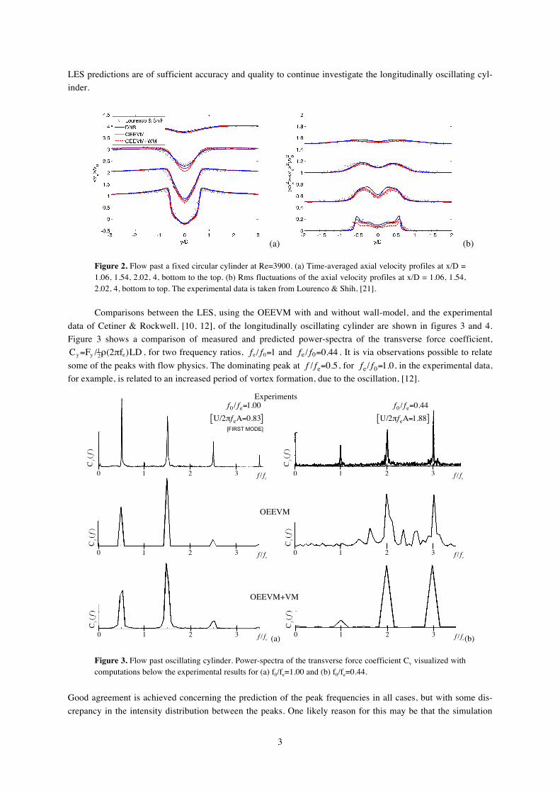
3

LES predictions are of sufficient accuracy and quality to continue investigate the longitudinally oscillating cyl-inder.

(a) (b)

Figure 2. Flow past a fixed circular cylinder at Re=3900. (a) Time-averaged axial velocity profiles at x/D = 1.06, 1.54, 2.02, 4, bottom to the top. (b) Rms fluctuations of the axial velocity profiles at x/D = 1.06, 1.54, 2.02, 4, bottom to top. The experimental data is taken from Lourenco & Shih, [21].

Comparisons between the LES, using the OEEVM with and without wall-model, and the experimental data of Cetiner & Rockwell, [10, 12], of the longitudinally oscillating cylinder are shown in figures 3 and 4. Figure 3 shows a comparison of measured and predicted power-spectra of the transverse force coefficient,

€

Cy=Fy /12ρ(2πfe)LD , for two frequency ratios,

€

fe / f0=1 and

€

fe / f0=0.44 . It is via observations possible to relate some of the peaks with flow physics. The dominating peak at

€

f / fe=0.5, for

€

fe / f0=1.0, in the experimental data, for example, is related to an increased period of vortex formation, due to the oscillation, [12].

[FIRST MODE]

!

0

!

1

!

2

!

3

!

0

!

1

!

2

!

3

!

f / fe

!

f / fe

!

f0/ f

e=1.00

U/2"feA=0.83[ ]

(a)

!

0

!

1

!

2

!

3

!

f / fe

!

f0/ f

e=0.44

U/2"feA=1.88[ ]

!

0

!

1

!

2

!

3

!

f / fe (b)

[FIRST MODE]

!

0

!

1

!

2

!

3

!

0

!

1

!

2

!

3

!

f / fe

!

f / fe

!

f0/ f

e=1.00

U/2"feA=0.83[ ]

(a)

!

0

!

1

!

2

!

3

!

f / fe

!

f0/ f

e=0.44

U/2"feA=1.88[ ]

!

0

!

1

!

2

!

3

!

f / fe(b)

Figure 3. Flow past oscillating cylinder. Power-spectra of the transverse force coefficient Cv visualized with computations below the experimental results for (a) f0/fe=1.00 and (b) f0/fe=0.44.

Good agreement is achieved concerning the prediction of the peak frequencies in all cases, but with some dis-crepancy in the intensity distribution between the peaks. One likely reason for this may be that the simulation

OEEVM+VM

OEEVM

Experiments

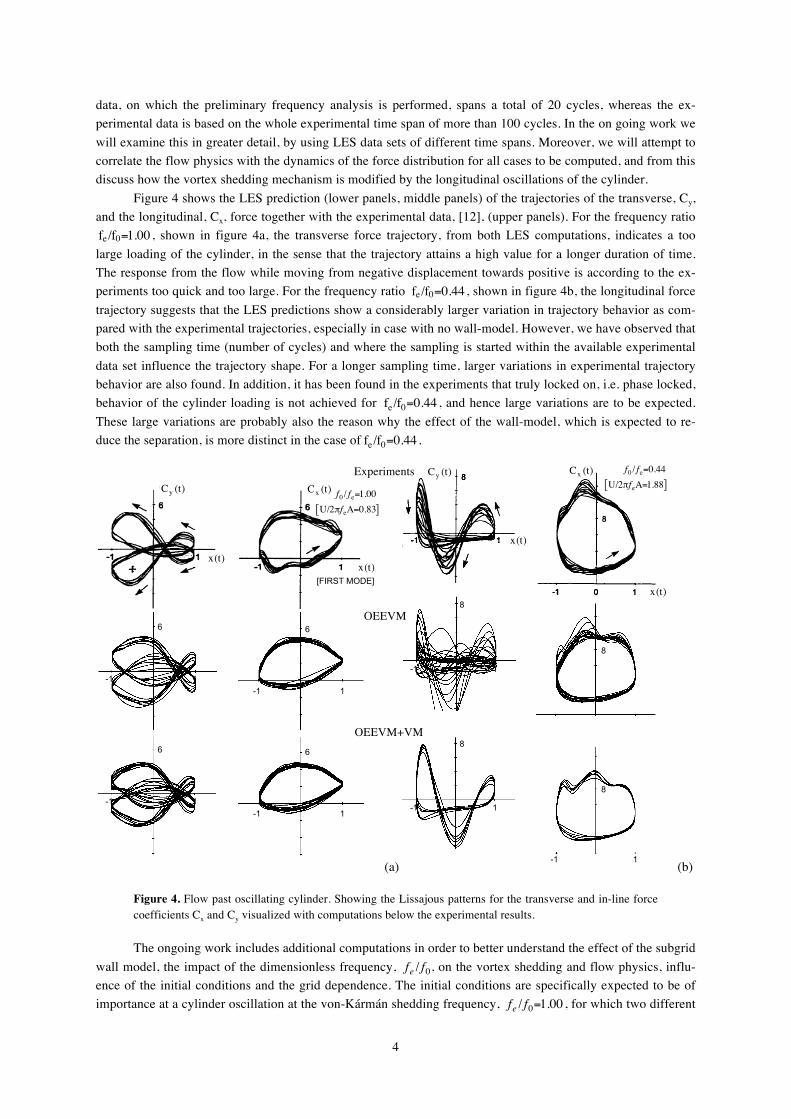
4

data, on which the preliminary frequency analysis is performed, spans a total of 20 cycles, whereas the ex-perimental data is based on the whole experimental time span of more than 100 cycles. In the on going work we will examine this in greater detail, by using LES data sets of different time spans. Moreover, we will attempt to correlate the flow physics with the dynamics of the force distribution for all cases to be computed, and from this discuss how the vortex shedding mechanism is modified by the longitudinal oscillations of the cylinder. Figure 4 shows the LES prediction (lower panels, middle panels) of the trajectories of the transverse, Cy, and the longitudinal, Cx, force together with the experimental data, [12], (upper panels). For the frequency ratio

€

fe/f0=1.00 , shown in figure 4a, the transverse force trajectory, from both LES computations, indicates a too large loading of the cylinder, in the sense that the trajectory attains a high value for a longer duration of time. The response from the flow while moving from negative displacement towards positive is according to the ex-periments too quick and too large. For the frequency ratio

€

fe/f0=0.44 , shown in figure 4b, the longitudinal force trajectory suggests that the LES predictions show a considerably larger variation in trajectory behavior as com-pared with the experimental trajectories, especially in case with no wall-model. However, we have observed that both the sampling time (number of cycles) and where the sampling is started within the available experimental data set influence the trajectory shape. For a longer sampling time, larger variations in experimental trajectory behavior are also found. In addition, it has been found in the experiments that truly locked on, i.e. phase locked, behavior of the cylinder loading is not achieved for

€

fe/f0=0.44 , and hence large variations are to be expected. These large variations are probably also the reason why the effect of the wall-model, which is expected to re-duce the separation, is more distinct in the case of

€

fe/f0=0.44 .

-1 1

6

!

Cy (t)

!

Cy (t)

!

x(t)

!

x(t)

-1 1

8

4

-4

6

6

[FIRST MODE]

!

f0/ f

e=1.00

U/2"feA=0.83[ ]

!

Cx (t)

!

Cx (t)

(a)

8

4

-4

0 12

-1 1

8

8

!

Cx (t)

!

Cx (t)

!

f0/ f

e=0.44

U/2"feA=1.88[ ]

!

Cy (t)

!

Cy (t)

!

x(t)

!

x(t)

(b)

-1 1

6

!

Cy (t)

!

Cy (t)

!

x(t)

!

x(t)

-1 1

8

4

-4

6

6

[FIRST MODE]

!

f0/ f

e=1.00

U/2"feA=0.83[ ]

!

Cx (t)

!

Cx (t)

(a)

8

4

-4

8

0 12

-1 1

8

-1 1

!

Cx (t)

!

Cx (t)

!

f0/ f

e=0.44

U/2"feA=1.88[ ]

!

Cy (t)

!

Cy (t)

!

x(t)

!

x(t)

(b)

Figure 4. Flow past oscillating cylinder. Showing the Lissajous patterns for the transverse and in-line force coefficients Cx and Cy visualized with computations below the experimental results.

The ongoing work includes additional computations in order to better understand the effect of the subgrid wall model, the impact of the dimensionless frequency,

€

fe / f0, on the vortex shedding and flow physics, influ-ence of the initial conditions and the grid dependence. The initial conditions are specifically expected to be of importance at a cylinder oscillation at the von-Kármán shedding frequency,

€

fe / f0=1.00 , for which two different

OEEVM

OEEVM+VM

Experiments

5

modes are experimentally observed, [12], this is also observed in some of our most recent computations. The flow physics for the first mode, displayed in figure 4a, resembles a von-Kármán vortex shedding, and is proba-bly best initialized from a fully developed flow. The second mode, which according to experiments is less sta-ble, with a lower probability of occurrence, exhibits simultaneous shedding and would probably require sym-metric initial conditions alternatively a very long simulation time. The flow physics will as a first step be exam-ined through instantaneous vorticity maps correlated in time with the transverse force coefficient, Cy, the cylin-der displacement x and the difference between the freestream velocity and the cylinder velocity.

References [1] Bishop R.E.D. & Hassan A.Y.; 1964, “The Lift and Drag Forces on a Circular Cylinder in a Flowing Fluid”, Proc. Roy. Soc. (London) A 277, p 32. [2] King R.; 1977, “A Review of Vortex Shedding Research and its Application”, Ocean Engineering, 4, p 141. [3] Fureby C.; 2008, “Towards Large Eddy Simulation in Engineering”, Prog. Aerospace Science, 44, p 381. [4] Sagaut P.; 2001, “Large Eddy Simulation for Incompressible Flows”, Springer Verlag. [5] Grinstein F. F., Margolin, L. G. & Rider W. J. (Eds); 2007, “Implicit Large Eddy Simulation Computing Turbulent Fluid Dynamics”, Cambridge University Press. [6] Nikitin N.V., Nicoud F. Wasistho B. Squires K.D. & Spalart P.R.; 2000, “An Approach to Wall Model-ing in Large Eddy Simulation”, Phys. Fluids, 12, p. 1629. [7] Wilcox, D.C.; 1993, “Turbulence Modeling for CFD”, DCW Industries. [8] Ongoren A. & Rockwell D.; 1988 “Flow structure from an oscillating cylinder, part 2, Mode competition in the near wake”, Journal of Fluid Mechanics, Vol 197, p 225-246 [9] Williamson C. H. K. & Roshko A.; 1988, “Vortex formation in the wake of an oscillating cylinder.”, Journal of Fluids and Structures, Vol. 2, pp 355-381 [10] Cetiner O. & Rockwell D.; 2001, ”Streamwise oscillations of a cylinder in a steady current. Part 1. Locked-on states of vortex formation and loading”, Journal of Fluid Mechanics, Vol 427, pp 1-28 [11] Cetiner O. & Rockwell D.; 2001, ”Streamwise oscillations of a cylinder in a steady current. Part 2. Free-surface effects on vortex formation and loading”, Journal of Fluid Mechanics, Vol 427, pp 29-59 [12] Cetiner O.; 1998, ”Flow Structure and Loading Due to an Oscillating Cylinder in a Steady Current”, Ph. D. dissertation. [13] Liefvendahl M. & Lillberg E.; 2005, “Computational Methods for Unsteady Fluid Force Predictions Us-ing Moving Mesh Large Eddy Simulations”, AIAA 2005-4144. [14] Lu X –Y & Dalton C.; 1996, “Calculation of the timing of vortex formation from an oscillating cylin-der.”, Journal of Fluids and Structures, Vol. 10, p 527-541 [15] Saritas M. & Cetiner O.; 2003, “Flow structure and loading due to an oscillating cylinder in steady cur-rent”, 7th International Symposium on Fluid Control [16] Fureby C. & Bensow R. 2007, “LES at Work: Quality Management in Practical LES”, Invited Review paper at QLES 2007. To appear in the Proceedings of the Conference, Springer Verlag. [17] Schumann U.; 1975, “Subgrid Scale Model for Finite Difference Simulation of Turbulent Flows in Plane Channels and Annuli, J. Comp. Phys., 18, p 376. [18] Fureby C.; 2007, “On LES and DES of Wall Bounded Flows”, Ercoftac Bulletin No 72, Marsh Issue. [19] Weller H.G., Tabor G., Jasak H. & Fureby C.; 1997, “A Tensorial Approach to CFD using Object Ori-ented Techniques“, Comp. in Physics, 12, p 629. [20] Demirdzic I. & Peric M.; 1988, “Space Conservation Law in Finite Volume Calculations of Fluid Flow”, International journal for numerical methods in fluids, Vol 8, p 1037-1050 [21] Jasak H. & Tukovic Z.; 2004, “Automatic Mesh Motion for the Unstructured Finite Volume Method”, Submitted to Journal of Computational Physics, http://www.h.jasak.dial.pipex.com/papers.html [22] Dröge M.; 2007, “Cartesian Grid Methods for Turbulent Flow Simulation in Complex Geometries”, Doctoral Dissertation, University of Groningen, [23] Lourenco L. & Shih .C; 1993, “Characteristics of the plane turbulent near wake of a circular cylinder. A particle image velocimetry study.” Data taken from [23] [24] Tremblay .F; 2001, “Direct and large-eddy simulation of flow around a circular cylinder at subcritical Reynolds number”, Doctoral dissertation, Technical University of Munich [25] Ma X., Karamons G-S. & Karniadakis G.E.; 2000, “Dynamics and low-dimensionality of a turbulent near wake”, Journal of Fluid Mechanics, 410, p. 29-65

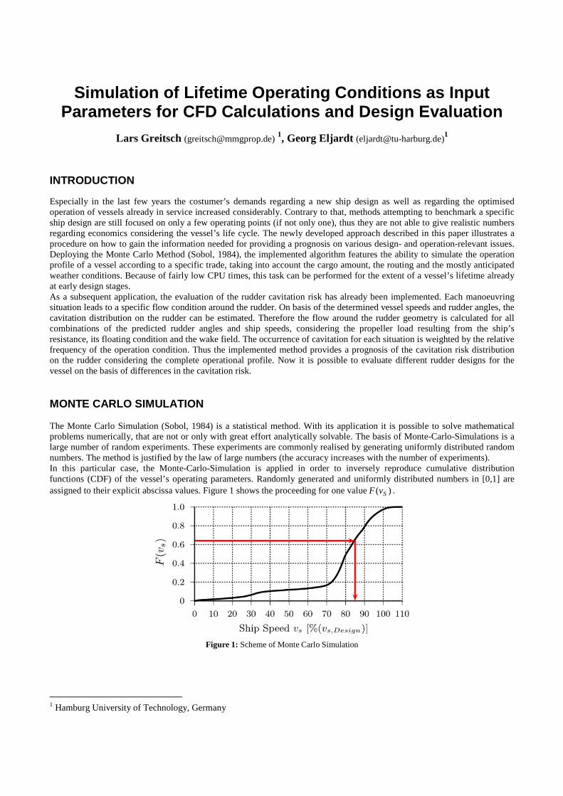
Simulation of Lifetime Operating Conditions as Input Parameters for CFD Calculations and Design Evaluation

Lars Greitsch (greitsch@mmgprop.de) 1, Georg Eljardt (eljardt@tu-harburg.de)1

INTRODUCTION Especially in the last few years the costumer’s demands regarding a new ship design as well as regarding the optimised operation of vessels already in service increased considerably. Contrary to that, methods attempting to benchmark a specific ship design are still focused on only a few operating points (if not only one), thus they are not able to give realistic numbers regarding economics considering the vessel’s life cycle. The newly developed approach described in this paper illustrates a procedure on how to gain the information needed for providing a prognosis on various design- and operation-relevant issues. Deploying the Monte Carlo Method (Sobol, 1984), the implemented algorithm features the ability to simulate the operation profile of a vessel according to a specific trade, taking into account the cargo amount, the routing and the mostly anticipated weather conditions. Because of fairly low CPU times, this task can be performed for the extent of a vessel’s lifetime already at early design stages. As a subsequent application, the evaluation of the rudder cavitation risk has already been implemented. Each manoeuvring situation leads to a specific flow condition around the rudder. On basis of the determined vessel speeds and rudder angles, the cavitation distribution on the rudder can be estimated. Therefore the flow around the rudder geometry is calculated for all combinations of the predicted rudder angles and ship speeds, considering the propeller load resulting from the ship’s resistance, its floating condition and the wake field. The occurrence of cavitation for each situation is weighted by the relative frequency of the operation condition. Thus the implemented method provides a prognosis of the cavitation risk distribution on the rudder considering the complete operational profile. Now it is possible to evaluate different rudder designs for the vessel on the basis of differences in the cavitation risk. MONTE CARLO SIMULATION The Monte Carlo Simulation (Sobol, 1984) is a statistical method. With its application it is possible to solve mathematical problems numerically, that are not or only with great effort analytically solvable. The basis of Monte-Carlo-Simulations is a large number of random experiments. These experiments are commonly realised by generating uniformly distributed random numbers. The method is justified by the law of large numbers (the accuracy increases with the number of experiments). In this particular case, the Monte-Carlo-Simulation is applied in order to inversely reproduce cumulative distribution functions (CDF) of the vessel’s operating parameters. Randomly generated and uniformly distributed numbers in [0,1] are assigned to their explicit abscissa values. Figure 1 shows the proceeding for one value )( SvF .

Figure 1: Scheme of Monte Carlo Simulation

1 Hamburg University of Technology, Germany

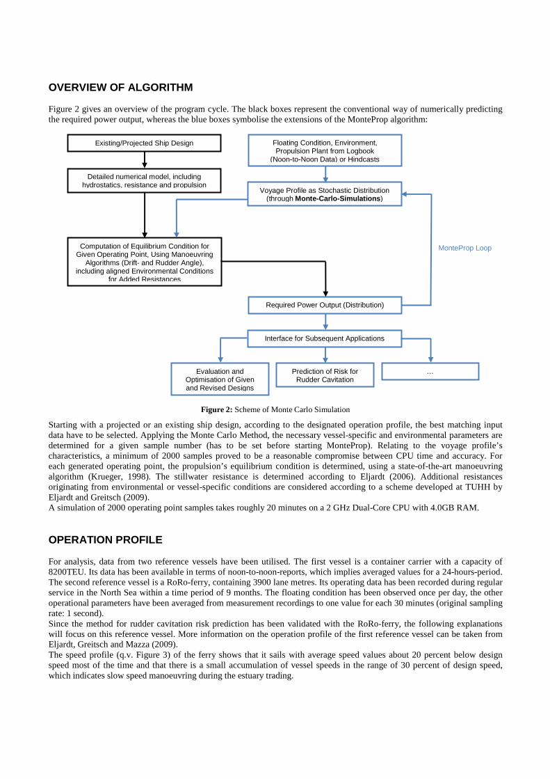
OVERVIEW OF ALGORITHM Figure 2 gives an overview of the program cycle. The black boxes represent the conventional way of numerically predicting the required power output, whereas the blue boxes symbolise the extensions of the MonteProp algorithm:

Figure 2: Scheme of Monte Carlo Simulation

Starting with a projected or an existing ship design, according to the designated operation profile, the best matching input data have to be selected. Applying the Monte Carlo Method, the necessary vessel-specific and environmental parameters are determined for a given sample number (has to be set before starting MonteProp). Relating to the voyage profile’s characteristics, a minimum of 2000 samples proved to be a reasonable compromise between CPU time and accuracy. For each generated operating point, the propulsion’s equilibrium condition is determined, using a state-of-the-art manoeuvring algorithm (Krueger, 1998). The stillwater resistance is determined according to Eljardt (2006). Additional resistances originating from environmental or vessel-specific conditions are considered according to a scheme developed at TUHH by Eljardt and Greitsch (2009). A simulation of 2000 operating point samples takes roughly 20 minutes on a 2 GHz Dual-Core CPU with 4.0GB RAM. OPERATION PROFILE For analysis, data from two reference vessels have been utilised. The first vessel is a container carrier with a capacity of 8200TEU. Its data has been available in terms of noon-to-noon-reports, which implies averaged values for a 24-hours-period. The second reference vessel is a RoRo-ferry, containing 3900 lane metres. Its operating data has been recorded during regular service in the North Sea within a time period of 9 months. The floating condition has been observed once per day, the other operational parameters have been averaged from measurement recordings to one value for each 30 minutes (original sampling rate: 1 second). Since the method for rudder cavitation risk prediction has been validated with the RoRo-ferry, the following explanations will focus on this reference vessel. More information on the operation profile of the first reference vessel can be taken from Eljardt, Greitsch and Mazza (2009). The speed profile (q.v. Figure 3) of the ferry shows that it sails with average speed values about 20 percent below design speed most of the time and that there is a small accumulation of vessel speeds in the range of 30 percent of design speed, which indicates slow speed manoeuvring during the estuary trading.

Existing/Projected Ship Design Floating Condition, Environment, Propulsion Plant from Logbook

(Noon-to-Noon Data) or Hindcasts

Voyage Profile as Stochastic Distribution (through Monte-Carlo-Simulations)

Computation of Equilibrium Condition for Given Operating Point, Using Manoeuvring

Algorithms (Drift- and Rudder Angle), including aligned Environmental Conditions

for Added Resistances

Required Power Output (Distribution)

Interface for Subsequent Applications

Evaluation and Optimisation of Given and Revised Designs

Prediction of Risk for Rudder Cavitation

…

Detailed numerical model, including hydrostatics, resistance and propulsion

MonteProp Loop

Figure 3: Probability Density Function (PDF) of Vessel Speed

Depending on the vessel’s designated route, the expected weather may differ significantly. In order to simulate the resulting added resistances as correct as possible, it is important to gather the necessary environmental data. This can either be done by observation (e.g. during the operation of similar vessels) or the data can be attained from hindcast weather reports. For the presented case, both ways have been employed. The wind force and the angle of attack (aoa) were recorded after observation, whereas the sea state and the correlation of wave height and period were hindcasted. The data was collected and averaged over a period of 10 years from 1990 to 1999 by the GKSS Research Centre, located in Geesthacht, Germany. It was provided in the course of the research project ADOPT (http://adopt.rtdproject.net/). Figure 4 shows the data points and the symbolic path of the vessel’s route across the Skagerrak and the North Sea between Gothenburg and Gent.

Figure 4: Route RoRo-ferry, Gothenburg – Gent Figure 5: CDF Wave Heights

Since the highlighted points along the route are rather equidistantly distributed, they have been taken into account with equal weighting. This has been done in order to determine one averaged CDF for each weather parameter (Figure 5). Worldwide sea state data can be obtained from Soeding (2001). E.g. the analysed container carrier operates on a liner service between Europe and Asia, thus Soeding’s data has been applied. Both parameters wind and sea state are correlated. This dependency has to be acknowledged when applying the subsequently described MonteProp-algorithm. During the analysis of the 8200-TEU-vessel, it proved to be feasible to incorporate the correlation through the following proceeding. At first, the wind force in Beaufort is determined as a floating point number. The sea state is derived afterwards by reducing the Beaufort number with a constant subtrahend of 1. For the described vessel and its voyage profile this procedure is slightly suboptimal, since the wind force’s statistical spread is wider than the sea state’s one (q.v. Figure 6).

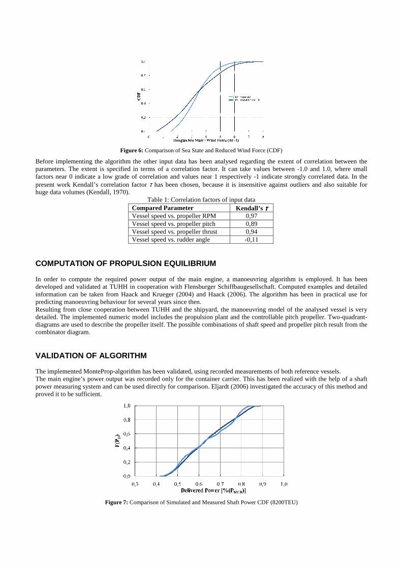
Figure 6: Comparison of Sea State and Reduced Wind Force (CDF)

Before implementing the algorithm the other input data has been analysed regarding the extent of correlation between the parameters. The extent is specified in terms of a correlation factor. It can take values between -1.0 and 1.0, where small factors near 0 indicate a low grade of correlation and values near 1 respectively -1 indicate strongly correlated data. In the present work Kendall’s correlation factor τ has been chosen, because it is insensitive against outliers and also suitable for huge data volumes (Kendall, 1970).

Table 1: Correlation factors of input data Compared Parameter Kendall’s ττττ Vessel speed vs. propeller RPM 0,97 Vessel speed vs. propeller pitch 0,89 Vessel speed vs. propeller thrust 0,94 Vessel speed vs. rudder angle -0,11

COMPUTATION OF PROPULSION EQUILIBRIUM In order to compute the required power output of the main engine, a manoeuvring algorithm is employed. It has been developed and validated at TUHH in cooperation with Flensburger Schiffbaugesellschaft. Computed examples and detailed information can be taken from Haack and Krueger (2004) and Haack (2006). The algorithm has been in practical use for predicting manoeuvring behaviour for several years since then. Resulting from close cooperation between TUHH and the shipyard, the manoeuvring model of the analysed vessel is very detailed. The implemented numeric model includes the propulsion plant and the controllable pitch propeller. Two-quadrant-diagrams are used to describe the propeller itself. The possible combinations of shaft speed and propeller pitch result from the combinator diagram. VALIDATION OF ALGORITHM The implemented MonteProp-algorithm has been validated, using recorded measurements of both reference vessels. The main engine’s power output was recorded only for the container carrier. This has been realized with the help of a shaft power measuring system and can be used directly for comparison. Eljardt (2006) investigated the accuracy of this method and proved it to be sufficient.

Figure 7: Comparison of Simulated and Measured Shaft Power CDF (8200TEU)

The diagram shown in Figure 7 compares the simulated and the measured shaft power CDFs of the 8200-TEU-class vessel. The function’s congruence is satisfactory, especially when considering the applied input data, its simplifications and the utilised methods with their incorporated numeric models. Other operation data, such as main engine revolution speed, propeller pitch and rudder angle have been compared to recorded data from the RoRo-Ferry. Figure 8 shows also good resemblance between measured and computed data.

Figure 8: Comparison of Simulated and Measured Parameters (RoRo-Ferry)

CAVITATION RISK ANALYSIS The cavitation risk for the rudder design is calculated as a risk distribution on the surface area of the rudder. For each discretised panel there is the calculated probability of cavitation occurrence within the whole operational profile. The cavitation prognosis is carried out by means of a panel code based on the potential flow theory. This allows very fast calculations and therefore the analysis of the large number of observed operation cases in a finite time period. The used CFD code takes into account the wake field of the observed vessel and the propeller slipstream, the latter of which is calculated with the lifting line method. The cavitation is calculated by comparing the local pressure with the vapour pressure of the passing water at the observed location. It is not distinguished between higher and lower pressure gradients. The interpretation of the results is carried out by a cavitation coefficient ccav as a saltus function which has the value 0 for non-cavitating situations of this panel and the value 1 in case of cavitation on the observed panel. In order to benchmark the cavitation risk for different regions on the rudder the cavitation pattern is calculated for each single simulated operating situation. The cavitation coefficient ccav therefore is a function of all major operational influences.

( )

larperpendicuaft at Draft :

flow Cross:

angleRudder :

rpmPropeller :

)(propeller ratiodiameter Pitch to:/

fraction wakeEffective:

speed Vessel:

:with

,,,,/,,

,

,

,,,,

=====

==

=

iAP

cross

i

i

eff

iS

iAPicrossiieffiSicav

T

v

n

DP

w

v

TvnDPwvfc

δ

δ

This leads to a safety against cavitation Scav for each panel

m

c

S

m

iicav

cav

∑=−= 1

,

1

As shown in Figure 9, a value of Scav = 1 specifies a 100 percent safety against cavitation for the observed panel in the range of operation situations. Resulting from the saltus function there can be no safety greater than 1. In the same manner a value of Scav = 0 indicates that the observed panel would cavitate in all operation situations. On basis of the cavitation risk distribution the benefit of a new rudder design can be evaluated directly. The capability of this approach has been presented at NuTTS (Greitsch, 2008) and 1st Symposium on Marine Propulsors (Greitsch and Eljardt, 2009).

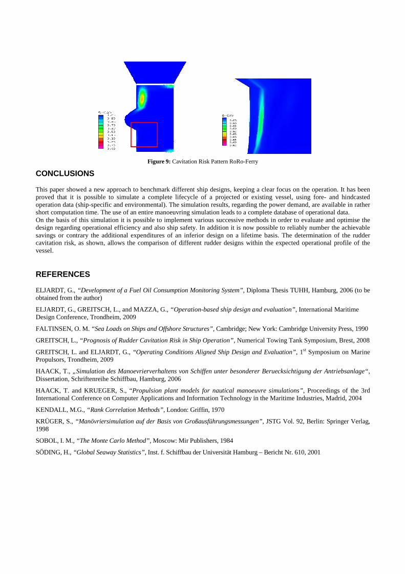
Figure 9: Cavitation Risk Pattern RoRo-Ferry

CONCLUSIONS This paper showed a new approach to benchmark different ship designs, keeping a clear focus on the operation. It has been proved that it is possible to simulate a complete lifecycle of a projected or existing vessel, using fore- and hindcasted operation data (ship-specific and environmental). The simulation results, regarding the power demand, are available in rather short computation time. The use of an entire manoeuvring simulation leads to a complete database of operational data. On the basis of this simulation it is possible to implement various successive methods in order to evaluate and optimise the design regarding operational efficiency and also ship safety. In addition it is now possible to reliably number the achievable savings or contrary the additional expenditures of an inferior design on a lifetime basis. The determination of the rudder cavitation risk, as shown, allows the comparison of different rudder designs within the expected operational profile of the vessel. REFERENCES ELJARDT, G., “Development of a Fuel Oil Consumption Monitoring System”, Diploma Thesis TUHH, Hamburg, 2006 (to be obtained from the author)

ELJARDT, G., GREITSCH, L., and MAZZA, G., “Operation-based ship design and evaluation”, International Maritime Design Conference, Trondheim, 2009

FALTINSEN, O. M. “Sea Loads on Ships and Offshore Structures”, Cambridge; New York: Cambridge University Press, 1990

GREITSCH, L., “Prognosis of Rudder Cavitation Risk in Ship Operation” , Numerical Towing Tank Symposium, Brest, 2008

GREITSCH, L. and ELJARDT, G., “Operating Conditions Aligned Ship Design and Evaluation” , 1st Symposium on Marine Propulsors, Trondheim, 2009

HAACK, T., „Simulation des Manoevrierverhaltens von Schiffen unter besonderer Beruecksichtigung der Antriebsanlage“ , Dissertation, Schriftenreihe Schiffbau, Hamburg, 2006

HAACK, T. and KRUEGER, S., “Propulsion plant models for nautical manoeuvre simulations”, Proceedings of the 3rd International Conference on Computer Applications and Information Technology in the Maritime Industries, Madrid, 2004

KENDALL, M.G., “Rank Correlation Methods”, London: Griffin, 1970

KRÜGER, S., “Manövriersimulation auf der Basis von Großausführungsmessungen”, JSTG Vol. 92, Berlin: Springer Verlag, 1998

SOBOL, I. M., “The Monte Carlo Method”, Moscow: Mir Publishers, 1984

SÖDING, H., “Global Seaway Statistics”, Inst. f. Schiffbau der Universität Hamburg – Bericht Nr. 610, 2001

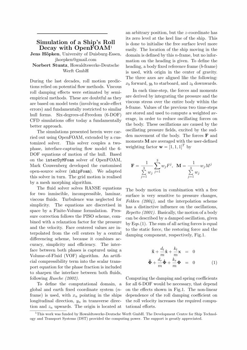
Simulation of a Ship’s RollDecay with OpenFOAM1

Jens Hopken, University of Duisburg-Essen,jhoepken@gmail.com

Norbert Stuntz, Howaldtswerke-DeutscheWerft GmbH

During the last decades, roll motion predic-tions relied on potential flow methods. Viscousroll damping effects were estimated by semi-empirical methods. These are doubtful as theyare based on model tests (involving scale-effecterrors) and fundamentally restricted to similarhull forms. Six-degrees-of-Freedom (6-DOF)CFD simulations offer today a fundamentallybetter approach.

The simulations presented herein were car-ried out using OpenFOAM, extended by a cus-tomized solver. This solver couples a two-phase, interface-capturing flow model the 6-DOF equations of motion of the hull. Basedon the interDyMFoam solver of OpenFOAM,Mark Couwenberg developed the customisedopen-source solver (shipFoam). We adaptedthis solver in turn. The grid motion is realisedby a mesh morphing algorithm.

The fluid solver solves RANSE equationsfor two inmiscible, incompressible, laminar,viscous fluids. Turbulence was neglected forsimplicity. The equations are discretised inspace by a Finite-Volume formulation. Pres-sure correction follows the PISO scheme, com-bined with a relaxation factor for the pressureand the velocity. Face centered values are in-terpolated from the cell centers by a centraldifferencing scheme, because it combines ac-curacy, simplicity and efficiency. The inter-face between both phases is captured using aVolume-of-Fluid (VOF) algorithm. An artifi-cial compressibility term into the scalar trans-port equation for the phase fraction is includedto sharpen the interface between both fluids,following Rusche (2002).

To define the computational domain, aglobal and earth fixed coordinate system (n-frame) is used, with xn pointing in the shipslongitudinal direction, yn in transverse direc-tion and zn upwards. The origin is located at

an arbitrary position, but the z-coordinate hasits zero level at the keel line of the ship. Thisis done to initialise the free surface level moreeasily. The location of the ship moving in thedomain is defined by this n-frame, but no infor-mation on the heading is given. To define theheading, a body fixed reference frame (b-frame)is used, with origin in the center of gravity.The three axes are aligned like the following:xb forward, yb to starboard, and zb downwards.

In each time-step, the forces and momentsare derived by integrating the pressure and theviscous stress over the entire body within theb-frame. Values of the previous two time-stepsare stored and used to compute a weighted av-erage, in order to reduce oscillating forces onthe body. These oscillations are caused by theoscillating pressure fields, excited by the sud-den movement of the body. The forces F andmoments M are averaged with the user-definedweighting factor w = [1, 1, 1]T by

F =1

3∑j=1

wj

3∑j=1

wjFj , M =

13∑

j=1wj

wjMj

The body motion in combination with a freesurface is very sensitive to pressure changes,Fekken (2004), and the interpolation schemehas a distinctive influence on the oscillations,Repetto (2001). Basically, the motion of a bodycan be described by a damped oscillation, givenby Eqs.(1). The sum of all acting forces is equalto the static force, the restoring force and thedamping component, respectively, Fig.1.

x +dt

mx +

kt

mx = 0

Φ +dr

mΦ +

kr

mΦ = 0 (1)

Computing the damping and spring coefficientsfor all 6-DOF would be necessary, that dependon the effects shown in Fig.1. The non-lineardependence of the roll damping coefficient onthe roll velocity increases the required compu-tational efforts.

1This work was funded by Howaldtswerke-Deutsche Werft GmbH. The Development Centre for Ship Technol-ogy and Transport Systems (DST) provided the computing power. The support is greatly appreciated.

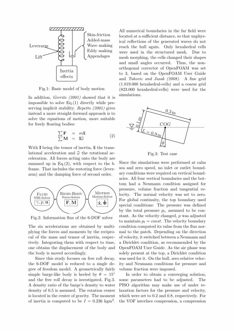
Inertiaeffects

Leverarm

Lift

Skin-frictionAdded-massWave makingEddy makingAppendages

Fig.1: Basic model of body motion

In addition, Gerrits (2001) showed that it isimpossible to solve Eq.(1) directly while pre-serving implicit stability. Repetto (2001) givesinstead a more straight-forward approach is tosolve the equations of motion, more suitablefor freely floating bodies:∑

F = mx∑M = Iω

(2)

With I being the tensor of inertia, x the trans-lational acceleration and ω the rotational ac-celeration. All forces acting onto the body aresummed up in Eq.(2), with respect to the b-frame. That includes the restoring force (lever-arm) and the damping force of second order.

FluidNSE-Solver

γ, p,u

Rigid-BodyForce-Solver

F,M

MotionMotion-Solver

x, Φ

Fig.2: Information flux of the 6-DOF solver

The six accelerations are obtained by multi-plying the forces and moments by the recipro-cal of the mass and tensor of inertia, respec-tively. Integrating them with respect to time,one obtains the displacement of the body andthe body is moved accordingly.

Since this study focuses on free roll decay,the 6-DOF model is reduced to a single de-gree of freedom model. A geometrically fairlysimple barge-like body is heeled by θ = 15

and the free roll decay is investigated, Fig.3.A density ratio of the barge’s density to waterdensity of 0.5 is assumed. The rotation centeris located in the center of gravity. The momentof inertia is computed to be I = 0.236 kgm2.

All numerical boundaries in the far field werelocated at a sufficient distance, so that unphys-ical reflections of the generated waves do notreach the hull again. Only hexahedral cellswere used in the structured mesh. Due tomesh morphing, the cells changed their shapesand small angles occurred. Thus, the non-orthogonal corrector of OpenFOAM was setto 3, based on the OpenFOAM User Guideand Tukovic and Jasak (2008). A fine grid(1.819.000 hexahedral-cells) and a coarse grid(823.000 hexahedral-cells) were used for thesimulations.

bCOG

θ

0.3m

0.1m

L = 0.9m

Fig.3: Test case

Since the simulations were performed at calmsea and zero speed, no inlet or outlet bound-ary conditions were required on vertical bound-aries. All four vertical boundaries and the bot-tom had a Neumann condition assigned forpressure, volume fraction and tangential ve-locity. The normal velocity was set to zero.For global continuity, the top boundary usedspecial conditions: The pressure was definedby the total pressure pt, assumed to be con-stant. As the velocity changed, p was adjustedto maintain pt = const. The velocity boundarycondition computed its value from the flux nor-mal to the patch. Depending on the directionof velocity, it switched between a Neumann anda Dirichlet condition, as recommended by theOpenFOAM User Guide. As the air phase wassolely present at the top, a Dirichlet conditionwas used for it. On the hull, zero relative veloc-ity and Neumann conditions for pressure andvolume fraction were imposed.

In order to obtain a converging solution,some parameters had to be adjusted. ThePISO algorithm may make use of under re-laxation factors for the pressure and velocity,which were set to 0.2 and 0.8, respectively. Forthe VOF interface compression, a compression

factor of 1 was chosen. The discretisation intime followed the Euler implicit method. Fromrun to run, the maximum Courant numberwas reduced successively, until the computa-tions finished with a stable result. As a result,the maximum Courant number was 0.1 for thesimulations with moving bodies. This valueturned out to improve the stability and con-vergence of the simulation.

-15

-10

-5

0

5

10

15

0 1 2 3 4 5

θ[

]

t [s]

finecoarse

Jung

Fig.4: Box barge’s roll decay

Fig.4 compares computed and experimental re-sults of Jung et al. (2006). Grid errors areshown to be small. During the first three os-cillations, no striking difference in the ampli-tude or period between the grids can be ob-served. After three periods, a small but no-table difference in the amplitude and periodcan be seen between both grids. The periodof the fine grid is smaller than the one of thecoarse gird, whereas the amplitude is higher atthe fine grid. A reason for this could be theeffect of numerical diffusion, whose influencecan be reduced by refining the mesh. This re-sults in a higher damping of the motion, whichincreases the roll-period and decreases the roll-amplitude. Furthermore the refinement of themesh leads to a smaller time-step, resulting ina finer temporal resolution of the motion. Thecause of this difference will be investigated fur-ther in the future. As can be seen in Fig.4, theroll-period of the fine grid is closer to the mea-sured one, than the roll-period of the coarsegrid. There is a significant difference in the rolldamping between the simulations and the ex-periments. The damping is more distinctive inthe experiments, increasing the difference be-tween the results with time. The major reasonfor this should be the negligence of turbulenceand the associated damping.

0

0.25

0.5

0.75

1

0 5 10 15 20 25 30

|S( ω

) |[m

2

rad s

]

ω [ rads ]

ωN

finecoarse

Jung

Fig.5: Amplitude spectrum of θ(t)

The natural roll frequency ωN is obtainedby performing a Fast Fourier Transformation(FFT) on the time history, Fig.5. The fre-quency at the maximum of |S(ω)| correspondsto the natural roll frequency. All values arenormalised with that maximum value. Table Icompares measure and computed natural rollfrequencies, comparing also to computed re-sults of Smith (2009). The measured spectrumis narrower than computed on the fine grid andwider than computed on the coarse grid. Thiscorresponds with a more frequent occurrence ofhigher roll frequencies in the simulation basedon the fine grid, than with the coarse grid andthe experiments. A reason for the deviationof the fine grid, compared to the coarse gridmaybe the different time-step size. The max-imum Courant number was specified and thatresults in a notable change of the total timesteps between both grids, Table I. The FFTis sensitive to the change of data points, espe-cially with a few total data points.

In order to analyse the damping of an os-cillation, a curve of extinction was used, Fig.6.There is no big difference between the dampingcharacteristics of the two grids and all valuesare linearly spread along the line of best fit.

Table I: Natural roll frequenciesGrid ωN [rad/s] error time-stepsExp. 6.78 – –coarse 6.55 3.44% 1581fine 6.88 1.53% 2603Smith 6.90 1.80% –

The amplitudes of the first oscillations showan accurate agreement between both grids, but

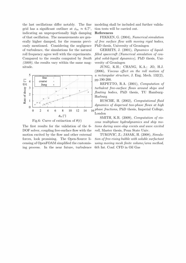
the last oscillations differ notably. The finegrid has a significant outliner at φm ≈ 6.7,indicating an unproportionally high dampingof that oscillation. The measurements are gen-erally higher damped, for the reasons previ-ously mentioned. Considering the negligenceof turbulence, the simulations for the naturalroll frequency agree well with the experiments.Compared to the results computed by Smith(2009), the results vary within the same mag-nitude.

0

1

2

3

4

5

0 2 4 6 8 10 12 14 16

Rat

eof

deca

ydφ dn

[]

φm []

finecoarse

Jung

Fig.6: Curve of extinction of θ(t)

The first results for the validation of the 6-DOF solver, coupling free-surface flow with themotion excited by the flow and other externalforces, look promising. The Open-Source li-censing of OpenFOAM simplified the customis-ing process. In the near future, turbulence

modeling shall be included and further valida-tion tests will be carried out.References

FEKKEN, G. (2004), Numerical simulationof free surface flow with moving rigid bodies,PhD thesis, University of Groningen

GERRITS, J. (2001), Dynamics of liquid-filled spacecraft (Numerical simulation of cou-pled solid-liquid dynamics), PhD thesis, Uni-versity of Groningen

JUNG, K.H.; CHANG, K.A.; JO, H.J.(2006), Viscous effect on the roll motion ofa rectangular structure, J. Eng. Mech. 132(2),pp.190-200.

REPETTO, R.A. (2001), Computation ofturbulent free-surface flows around ships andfloating bodies, PhD thesis, TU Hamburg-Harburg

RUSCHE, H. (2002), Computational fluiddynamics of dispersed two-phase flows at highphase fractions, PhD thesis, Imperial College,London

SMITH, K.R. (2009), Computation of vis-cous multiphase hydrodynamics and ship mo-tions during wave-slap events and wave excitedroll, Master thesis, Penn State Univ.

TUKOVIC, Z.; JASAK, H. (2008), Simula-tion of free-rising bubble with soluble surfactantusing moving mesh finite volume/area method,6th Int. Conf. CFD in Oil Gas

Investigating the Flexibility of Twin Screw Vessels with Various Propulsion Concepts using CFD

Tobias Huuva and Magnus Pettersson, Berg Propulsion Technology AB

Email: tobias.huuva@bergpropulsion.com

Introduction Many ships are today equipped with a single screw propulsion system, but as the demands on high efficiency, as well as increased flexibility and redundancy becomes stronger, many designers and ship owners are looking towards multi screw propulsion systems. With a multi‐, or usually, twin screw propulsion system the propulsion efficiency can become higher as compared to a single screw propulsion system. To take advantage of this higher propulsive efficiency the hull should be designed to account for the two propellers by having a twin skeg aft body. The twin skeg is used to direct the boundary layer from the hull into the propeller, giving higher hull efficiency as well as higher overall efficiency, as compared with a single skeg hull with a twin screw propulsion system. Comparing a single screw ship with a twin screw ship can be slightly more complicated but a simple attempt will be made here. The efficiency is not the only factor important in discussing single screw versus twin screw propulsion systems, also other factors needs to be considered, flexibility of the vessel is one such factor. On a vessel with a single propeller the speed can only be lowered by decreasing the power from the engine. For a fix pitch propeller this is performed by lowering the rate of revolution of the propeller and for a controllable pitch it is performed by either only lowering the pitch or by combining a lower pitch with a lover rate of revolution, called combinatory mode. When the speed is lowered in this way both engine and the propeller are working in an off design condition and the overall efficiency of the propulsion system can be lowered significantly. In a twin screw propulsion system the speed of the vessel can be lowered in a different way, by closing one propulsion line and let the remaining propeller drive the ship. The closed propulsion line can now be treated in two different ways. One is to lock the propeller shaft and one is to let the propeller rotate freely. If the propeller shaft is locked, a break is needed on the shaft line to have it fixed. If on the other hand the shaft is rotated freely a clutch is needed to disconnect the propeller from the engine. This clutch is usually located on the gear box or as a shaft clutch which is more complicated. If the shaft line cannot be locked or clutched out it is not possible to drive the ship in this way and the only possibility to lower the speed of the ship is to lower the power from the engines and letting both propellers drive the ship. Both of these options, locked and clutched out propeller, are in principle possible to perform with both fixed pitch (FP) and controllable pitch (CP) propellers, with an advantage for the CP propeller since the pitch can be adjusted for lowest possible resistance. Commonly a CP propeller has a pitch range from full ahead at about 30 degrees, which is somewhat higher than what a fix pitch propeller would have, to full astern at about ‐25 degrees. There exists also a third alternative and this comes in when the CP hub has the possibility to feather the blades, i.e. the blades can be set in 90 degree pitch being parallel to the flow. Not all CP hubs have this possibility and only very few have it included in a standard hydraulic hub. Having this CP‐propeller, with or without the possibility to feather the blades, turned off in a twin screw setup, the highest resistance would be when the

blades are in zero pitch position, because then the projected area is the largest, while the lowest resistance will be investigated in the proceeding sections.

Computational settings To investigate the differences of driving the ship in these different configurations a principle ship is used. This principle vessel is a typical ship where this type of setup could be of interest and possibly be of use. It is a 100 m tanker with 3.6 meter propeller driven by 3200 kW. This tanker has either a single screw propulsion system with a single skeg aft‐body, or a twin screw propulsion system with twin skeg aft body. The power is, for simplicity as described later, divided over two engines each of 1600 kW. This type of ship would typically have a maximum speed of 13 knots at 3200 kW and by using a simple approximation that the power relates to the speed as · , where in this case

0.112 / , this vessel would run with approximately 10.9 knots at 1600 kW. The computations are only performed for the propeller not in use, the running propeller are assumed to drive the ship in the correct speed and is not influencing the simulated propeller. The blades have a medium skew of about 30 degrees and an expanded blade area ratio (EAR) of about 0.4. The propeller is located in the wake of the ship and the speed of the water approaching the propeller is

· . For a twin skeg tanker hull, such as the principle ship used here, the wake fraction is assumed to be 0.22 giving 8.5 . The computation is performed in open water setting using steady Reynolds Averaged Navier Stokes (RANS) and Multiple Reference Frame (MRF). The RANS equations are solved using the open source library OpenFOAM, using a realizable k‐epsilon model and a blended scheme, using about 80% second order and 20 % first order numeric. The mesh is fully tetrahedral with a prism layer around the wall boundaries containing about 5,000,000 cells for the full propeller. The y+ value of the first cell is about 100 and consequently a wall handling technique is used based on the law of the wall. The pitch of the blades is set in two conditions, one is the feathered condition, and one is in design condition pitch, corresponding to 80% of full ahead pitch for a non‐feathered hub. Two computations are made with the propeller locked, one for each pitch setting and one computation is performed with the propeller rotating and the pitch in design condition. The rotating case is referred to as self milling condition when the momentum from the water on the propeller levels the losses in the shaft line and the gear box and one case called driven milling when the thrust from the propeller is zero.

Result A basic principle in propulsion theory is that the efficiency of the propeller will be increased if the diameter is increased and the rate of revolution is decreased. The same principle appears when diameter of the propeller is kept constant and the power to the propeller is decreased, as is the case when the power is divided over two propellers instead of on a single propeller. Splitting the power over two propellers will imply that the loading on the propeller will be lower and consequently the blade area can be reduced without increasing the risk of erosive cavitation. In figure 1 the open water propulsion efficiency of a single screw relative to a twin screw vessel is compared. For the single screw vessel a wake fraction of 0.27 is assumed and for the twin screw tanker the wake fraction is assumed to be 0.22. Using the same cavitation margin [1] and varying the rate of revolution to find the optimum efficiency of the propeller, based on the Wagningen b‐screw series [1] with a full scale correction of 3%, it is found that the difference in open water propulsion

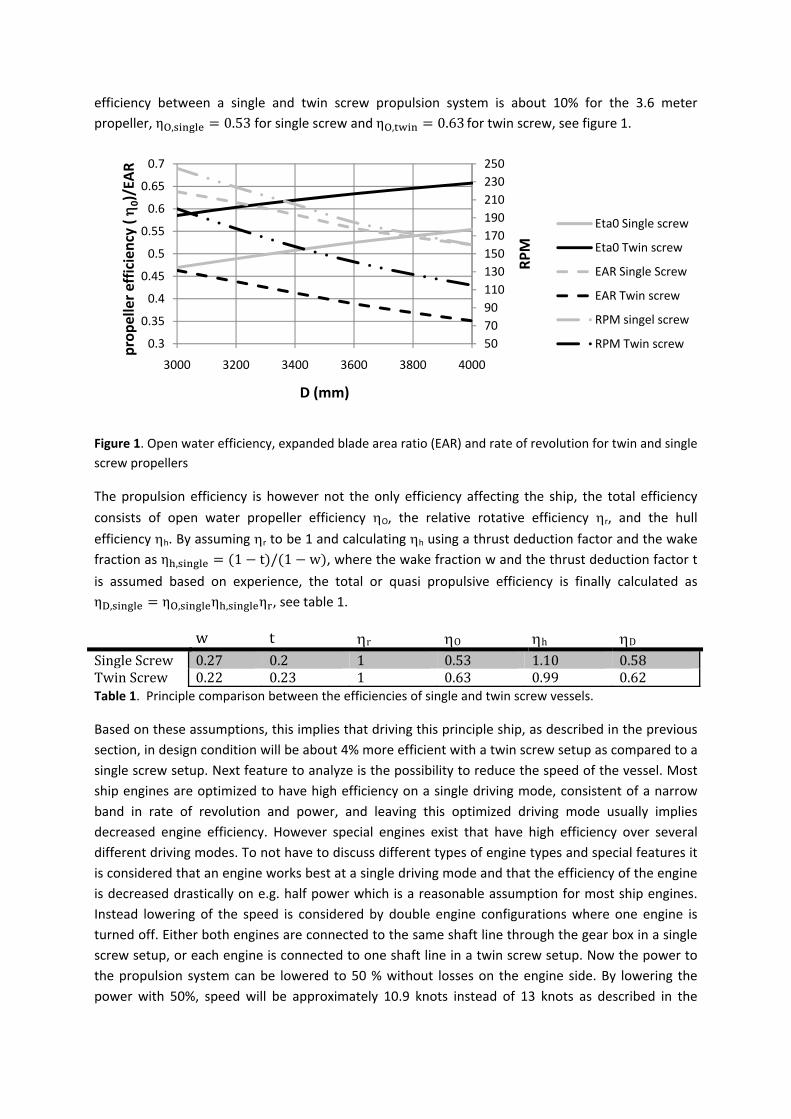
efficiency between a single and twin screw propulsion system is about 10% for the 3.6 meter propeller, ηO, 0.53 for single screw and ηO, 0.63 for twin screw, see figure 1.

Figure 1. Open water efficiency, expanded blade area ratio (EAR) and rate of revolution for twin and single screw propellers

The propulsion efficiency is however not the only efficiency affecting the ship, the total efficiency

consists of open water propeller efficiency ηO, the relative rotative efficiency ηr, and the hull

efficiency ηh. By assuming ηr to be 1 and calculating ηh using a thrust deduction factor and the wake fraction as η , 1 t / 1 w , where the wake fraction w and the thrust deduction factor t

is assumed based on experience, the total or quasi propulsive efficiency is finally calculated as ηD, ηO, η , η , see table 1.

w t ηr ηO ηh ηD Single Screw 0.27 0.2 1 0.53 1.10 0.58 Twin Screw 0.22 0.23 1 0.63 0.99 0.62 Table 1. Principle comparison between the efficiencies of single and twin screw vessels.

Based on these assumptions, this implies that driving this principle ship, as described in the previous section, in design condition will be about 4% more efficient with a twin screw setup as compared to a single screw setup. Next feature to analyze is the possibility to reduce the speed of the vessel. Most ship engines are optimized to have high efficiency on a single driving mode, consistent of a narrow band in rate of revolution and power, and leaving this optimized driving mode usually implies decreased engine efficiency. However special engines exist that have high efficiency over several different driving modes. To not have to discuss different types of engine types and special features it is considered that an engine works best at a single driving mode and that the efficiency of the engine is decreased drastically on e.g. half power which is a reasonable assumption for most ship engines. Instead lowering of the speed is considered by double engine configurations where one engine is turned off. Either both engines are connected to the same shaft line through the gear box in a single screw setup, or each engine is connected to one shaft line in a twin screw setup. Now the power to the propulsion system can be lowered to 50 % without losses on the engine side. By lowering the power with 50%, speed will be approximately 10.9 knots instead of 13 knots as described in the

507090110130150170190210230250

0.3

0.35

0.4

0.45

0.5

0.55

0.6

0.65

0.7

3000 3200 3400 3600 3800 4000

RPM

prop

eller efficiency ( η

0)/EAR

D (mm)

Eta0 Single screw

Eta0 Twin screw

EAR Single Screw

EAR Twin screw

RPM singel screw

RPM Twin screw

previous section. Again the Wagningen B‐screw series can be consulted and the open water efficiency of the two propulsion cases can be estimated. There are two different scenarios that need to be considered, one where the propulsion system is working on combinatory drive, i.e. that both pitch and engine revolutions per minute (rpm) is varied to find highest possible efficiency, and one where the engine is working on fixed rpm, commonly when e.g. a shaft generator is connected to the gearbox. Further the thrust deduction needs to be revised, on a single screw ship the thrust deduction factor can be considered to be constant when the speed is lowered, but on the twin screw ship the total thrust deduction should go down considerably when the vessel is driven on only a single propeller. The hull will only be subjected to thrust deduction on half of the hull, while the other half of the vessel is not affected by any thrust deduction. Consequently a simple formula for the thrust deduction on a twin screw ship only driven by a single propeller will be _

_ /2. The wake fraction and the relative rotative efficiency are considered to remain constant when the speed is lowered, see table 2.

w t ηr ηO ηh ηD n (rpm) Single fix rpm 0.27 0.2 1 0.50 1.10 0.55 185Single combinatory 0.27 0.2 1 0.55 1.10 0.61 150Twin fix rpm 0.22 0.115 1 0.56 1.13 0.63 141Twin combinatory 0.22 0.115 1 0.56 1.13 0.63 150Table2. Principle comparison between the efficiencies of single and twin screw vessels driven on half power using a single engine at design condition and one propeller in all cases.

What now is left to estimate is the induced drag of the propeller that is not in use in the twin screw setup. By using CFD the influence of the different alternatives described earlier can be estimated and efficiency losses can be calculated by / , where is the efficiency loss due to the

propeller not in use and is the power needed to drive the propeller, which is not in use, through

the water. The appended resistance is calculated for a locked propeller in feathered position as well as in design position, corresponding to approximately 80% of full pitch. The self milling and driven milling conditions are considered by varying the rate of revolution of the propeller until the propeller levels the losses in the shaft line and the gear box, corresponding to a self‐milling propeller, and zero thrust, corresponding to a driven milling propeller, are found. The losses that needs to be matched by the propeller in the self milling case is assumed to be 3% of full power, i.e. 47 kW. These calculated values can now be compared to the power needed to drive the ship by multiplying the resistance of the propeller with the speed of the advancing water, and the efficiency loss can be found by dividing this appendage power with the delivered power, the result can be found in table 3.

R (kN) M (kNm) n (rpm) Vs (kts) Shaft (kW) Power (kW)

Driven Milling 0 7 64 10 47 95 0.06Self Milling 27 0 55 10 0 139 0.09Locked‐Feathered

5 0 0 10 0 25.5 0.015

Locked‐design 51 0 0 10 0 262 0.16Table 3. Added resistance and efficiency loss for the propeller not in use on the twin screw vessel at half power, computed with CFD. Shaft corresponds to losses in shaft line for the driven milling case.

Table 3 shows that the efficiency loss due to the propeller not in use varies between 2% and 16%, where the feathered propeller as expected has a much higher efficiency as compared to the other

cases. The only difference in these cases is that the driven milling case has zero resistance, but the shaft is on the other hand driven by a specific power to achieve this zero resistance of the propeller. The torque and thrust to the propeller can be seen in figure 2, showing that the driven and self milling points are located very close to each other. In this graph 0 rpm corresponds to the locked design condition, while 136 rpm corresponds to the design condition and the computed thrust and torque correspond rather well with the thrust and torque computed from the Wagningen B screw series.

Figure 2. Propeller thrust and torque at varying propeller rpm, zero torque gives self milling condition and zero thrust gives driven milling condition, computed with CFD.

Full scale test To perform some check that the calculated values are reasonable, some measurements where performed on the ship STENA Freighter. STENA Freighter is a quite different ship as compared to the vessel used here but at least some principles could be found during the simple tests. The vessel is driven by two propellers each connected to two engines of each 5670 kW, giving a total 22680 kW. In normal conditions only two of the engines are in use at 85% of maximum continuous rate (MCR), one engine connected to each shaft line, and a shaft generator of about 700 kW to one of the gear boxes. At this condition the STENA Freighter runs at approximately 18.5 knots, using the simple approximation introduced earlier would imply that the speed would scale as 0.087 , where the power P in kW and the speed Vs is given in knots. The tests were performed using one, two and three engines, with the shaft generator running. The propeller of STENA Freighter is larger as compared to the principle propeller used here, the diameter of the propeller about is 1.7 times higher and the blade area is about 1.5 times bigger as compared to the propeller described in the previous section. This implies that forces and powers presented in table 3 should be increased by 1.5 · 1.7 4.2 times. Using only one propeller with one engine at 85% MCR and the shaft generator, and self‐mill the other propeller, the vessel performed about 13.5 knot. As described above the vessel performed 18.5 knots using two propellers with two engines at 85% MCR and the shaft generator, including also a third engine at 85% MCR made the vessel travel at about 20.5 knots. Using these points together with the zero point and maximum speed of the vessel at full power of

‐150

‐100

‐50

0

50

100

150

200

250

300

‐60

‐40

‐20

0

20

40

60

80

100

120

0 20 40 60 80 100 120 140

Thrust [kN]

Torque

[kNm]

Rotational speed [rev/min]

Torque

Thrust

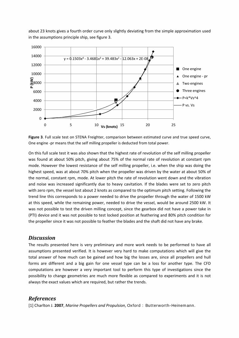
about 23 knots gives a fourth order curve only slightly deviating from the simple approximation used in the assumptions principle ship, see figure 3.

Figure 3. Full scale test on STENA Freighter, comparison between estimated curve and true speed curve, One engine ‐pr means that the self milling propeller is deducted from total power.

On this full scale test it was also shown that the highest rate of revolution of the self milling propeller was found at about 50% pitch, giving about 75% of the normal rate of revolution at constant rpm mode. However the lowest resistance of the self milling propeller, i.e. when the ship was doing the highest speed, was at about 70% pitch when the propeller was driven by the water at about 50% of the normal, constant rpm, mode. At lower pitch the rate of revolution went down and the vibration and noise was increased significantly due to heavy cavitation. If the blades were set to zero pitch with zero rpm, the vessel lost about 2 knots as compared to the optimum pitch setting. Following the trend line this corresponds to a power needed to drive the propeller through the water of 1500 kW at this speed, while the remaining power, needed to drive the vessel, would be around 2500 kW. It was not possible to test the driven milling concept, since the gearbox did not have a power take in (PTI) device and it was not possible to test locked position at feathering and 80% pitch condition for the propeller since it was not possible to feather the blades and the shaft did not have any brake.

Discussion The results presented here is very preliminary and more work needs to be performed to have all assumptions presented verified. It is however very hard to make computations which will give the total answer of how much can be gained and how big the losses are, since all propellers and hull forms are different and a big gain for one vessel type can be a loss for another type. The CFD computations are however a very important tool to perform this type of investigations since the possibility to change geometries are much more flexible as compared to experiments and it is not always the exact values which are required, but rather the trends.

References [1] Charlton J. 2007, Marine Propellers and Propulsion, Oxford : Butterworth-Heinemann.

y = 0.1503x4 ‐ 3.4681x3 + 39.483x2 ‐ 12.063x + 2E‐08

0

2000

4000

6000

8000

10000

12000

14000

16000

0 5 10 15 20 25

P (kW)

Vs (knots)

One engine

One engine ‐ pr

Two engines

Three engines

P=k*Vs^4

P vs. Vs

Effects of breaking intensity on wave breaking dynamics

Alessandro Iafrati, INSEAN, Rome, Italy, E-mail: a.iafrati@insean.it

1. INTRODUCTION

The breaking of ocean waves plays a fundamental role on momentum, energy and gas transfer between airand water. The phenomenon is characterized by a broad range of length scales. Moderate winds blowingover an otherwise flat sea surface give rise to waves of few centimeters wavelength. At such short scalesthe stabilizing action of gravity and surface tension dominate over the disrupting effect of the turbulence(Brocchini and Peregrine, 2001). The breaking is of the spilling type with essentially no air entrappedand vorticity is induced in water as a consequence of the viscous effects taking place beneath the bulge(Qiao and Duncan, 2001; Iafrati and Campana, 2005). In open ocean, where strong winds act over longfetches, the breaking is much more violent. Rather large jets develop about the wave crest and plungeonto the water surface entrapping large air cavities, with a strong turbulence field leading to a significantamount of drops, sprays and bubbles.

Many experimental investigation have been done with the aim of analyzing the breaking dynamics.Studies in connection with the spilling breaking case are given in Qiao and Duncan (2001). A ratherwide investigation of the plunging breaking event is given in Rapp and Melville (1990). More recently,Melville et al. (2002) performed similar studies by using more sophisticated measurement techniques.

Despite so many experimental studies, there are several issues which are not yet fully understood.Accurate analyses of the early stage after the onset of breaking are rather challenging because of thelight scattering operated by bubble clouds. Experimental measurements indicate that most of the energydissipated by the breaking process is lost within few wave periods after the breaking onset whereas fieldmeasurements are available only after three wave periods from the breaking onset, when large air bubbleshave degassed (Melville et al., 2002).

Numerical modeling of the two-fluids flow of air and water represents a good, non-intrusive, investi-gation tool which can help in understanding some of the unresolved issues. In this paper the breaking ofperiodic wave trains with different initial steepnesses is simulated numerically. The numerical approachis based on a Navier-Stokes solver coupled with a Level-Set technique for the interface capturing. At thepresent stage of the development results are limited to two-dimensions and the Reynolds number of thenumerical simulations is one order of magnitude smaller than the actual one. It is discussed in Iafrati(2009) that the above assumptions, although rather strong, do not play an important role up to abouthalf wave period after the breaking onset. Results are discussed in terms of energy dissipation, inducedcirculation in water, momentum transfer, air entrapment and degassing.

2. NUMERICAL MODEL

The unsteady two-fluids flow of air and water is approximated as that of a single incompressible fluidwhose density and viscosity vary smoothly across the interface. The problem is governed by the Navier-Stokes equations

∇ · u = 0

Du

Dt= −1

ρ∇p + f +

1ρ∇ ·

[µ(∇u +∇uT )

]+ σκνδ(x− xs) , (1)

where ρ and µ are the local values of density and dynamic viscosity, respectively. In equation (1) p is thepressure, f denotes the mass forces, σ is the surface tension coefficient, κ is the local curvature of theinterface and ν is the unit normal vector at the interface oriented toward the air. The term δ(x − xs)represents the Dirac function which is zero out of the interface location xs.

The system of Navier-Stokes equations is written in generalized variables and discretized onto a nonstaggered grid in a way similar to that proposed by Zang et al. (1994). The system is solved througha fractional step approach: the momentum equation is advanced in time by neglecting pressure terms(Predictor step) whose effects are successively reintroduced by enforcing the continuity of the velocityfield (Corrector step). The diagonal part of the dominating diffusive terms is accounted implicitly witha Crank-Nicolson scheme, whereas the other viscous terms, related to the non uniformity of the viscosity

and to the grid distortion, are computed explicitly. A low-storage, three-steps Runge-Kutta is adoptedfor the explicit terms. The Poisson equation for the pressure corrector term is solved with a Biconjugategradient stabilized (BiCGstab) algorithm (van der Vorst, 1992).

The interface is captured through a Level-Set algorithm. The signed distance d from the interface isreinitialized at each step and is convected with the transport equation:

∂d

∂t= −u · ∇d ,

which ensure that all particles belonging to the free surface (d = 0) remain on it, according to thekinematic boundary condition. The surface tension contribution to the momentum equation is approxi-mated by a continuum model as suggested in Brackbill et al. (1992). A more extensive discussion of thenumerical model and its validation and verification is given in Iafrati and Campana (2005).

3. INITIAL FREE–SURFACE PROFILE

A periodic wave profile is initialized as

η(x, 0) =a

λ

(cos(kx) +

12ε cos(2kx) +

38ε2 cos(3kx)

), (2)

where k = 2π/λ is the fundamental wavenumber, ε = ak is the initial wave steepness and λ is thefundamental wavelength. The fundamental wavelength is taken as reference value for lengths, whereasUr =

√λg is assumed as reference value for the velocities. The initial velocity field in water is assigned

asu = Ωa exp(ky) cos(kx) , v = Ωa exp(ky) sin(kx) , (3)

where Ω =√

gk(1 + ε2) accounts for the nonlinear correction (Whitham, 1974).Note that equation (2) is not exactly a third order Stokes wave as the secular term is missing (Grue

et al., 2003). The purpose of the present paper is to generate breaking waves of different intensities andto see in which way intensity of the breaking process affects the breaking dynamics. In this regard thelack of the secular term has only a minor effect on the results, as it is discussed in Iafrati (2009).

At the beginning of the simulation the flow in air is assumed to be at rest, and the motion occurring inair in the later stage is induced by the momentum exchange at the interface operated by both tangentialand normal stresses. No-slip boundary conditions are assigned at the top and bottom boundaries. As thewater depth is of the order of half of the fundamental wavelength, that choice does not affect remarkablythe dynamics of the breaking process (Chen et al., 1999). Also, for such wavelength-depth ratio, theenergy loss by bottom friction is essentially negligible (Lighthill, 1978). In all cases it is assumed

We = g1/2λ

√ρw

σ= 100 ,

which corresponds to water waves of about 30 centimeters wavelength. For such wavelength the Reynoldsnumber is

Re =ρwg1/2λ3/2

µw' 4.4× 105 ,

which is too high, even for a two-dimensional solver, for all the scales generated by the breaking processto be accurately resolved. For this reason numerical simulations are carried out at Re = 104. Someconsiderations concerning with the role played by this assumption are given in the following. The densityratio is assumed to be equal to the real one for air and water, which is ρa/ρw = 0.00125, whereas theviscosity ratio is µa/µw = 0.04, the same used by Chen et al. (1999).

The computational domain is one fundamental wavelength wide and one fundamental wavelengthhigh, that is x, y ∈ [−0.5, 0.5], and it is discretized by 512 × 512 grid cells, uniformly spaced. For thecase with ε = 0.65, large drops with high upward velocity components are generated by the plunging ofthe jet and a higher computational domain, with y ∈ [−0.5, 1.5] and a 512 × 1024 grid, is used. In thenumerical simulations it is assumed δP = δT = 0.005 which means that density and viscosity jumps andsurface tension forces are spread across a region which is about five grid cells thick. As lengths are scaledby the wavelength, for a 30 centimeters wave the cell size is about 0.6 millimeters and the thickness ofthe transition region corresponds to 3 millimeters. This physical value is used in the next section in orderto relate the results with the experimental findings.

In order to investigate to which extent the initial wave steepness changes the phenomena involvedin the breaking event, numerical simulations are carried out by varying ε in the range 0.2 to 0.65. It isfound that the breaking is of the spilling type for ε = 0.33 and ε = 0.35 whereas it is of the plungingtype for ε > 0.37.

x

y

-0.4 -0.2 0 0.2 0.4 0.6-0.3

-0.2

-0.1

0

0.1

x

y

-0.4 -0.2 0 0.2 0.4 0.6-0.3

-0.2

-0.1

0

0.1

Figure 1: Different vorticity production mechanisms in spilling and plunging breaking waves.Vorticity contours for ε = 0.35 and ε = 0.60 are drawn in the upper and lower picture,respectively.

4. NUMERICAL RESULTS

A first important change induced by the different breaking intensity concerns the vorticity productionmechanism. As it is shown in Fig. 1, for weak intensities surface tension prevents the formation ofthe plunging jet which is replaced by the development of a bulge about the wave crest. A shear layerdevelops at the breaker toe as a result of the interaction between the fluid inside the bulge and theupslope motion of the fluid beneath (Qiao and Duncan, 2001; Iafrati and Campana, 2005). For strongerbreaking intensities, the circulation is induced in water because of the topological change taking placewhen the plunging jet impinges onto the free surface ahead. In this sense viscosity has a minor role as itonly contributes to diffuse the vorticity whereas the total amount of circulation depends on the breakingintensity mainly (Iafrati, 2009).

0.2

0.3

0.4

0.5

0.6

0.7

0.8

0.9

1

0 2 4 6 8 10 12 14 16

ET (

t) /

ET (

0)

t

0.30

0.35

0.370.40

0.2

0.3

0.4

0.5

0.6

0.7

0.8

0.9

1

0 2 4 6 8 10 12 14 16

ET (

t) /

ET (

0)

t

0.400.50 0.55

0.60 0.65

55

%

44

%

Figure 2: Time histories of the total wave energy nondimensionalized by the initialenergy content ET (0). The left picture indicates how the energy dissipation increaseschanging because of the breaking occurrence. The right picture indicates that, in allthe plunging breaking cases, the energy fraction dissipated by the breaking is nearlyindependent of the breaking intensity.

Because of the stronger vorticity generated in the plunging breaking case, the energy fraction dissi-pated by breaking process is also larger (Rapp and Melville, 1990). This is can be also seen from the

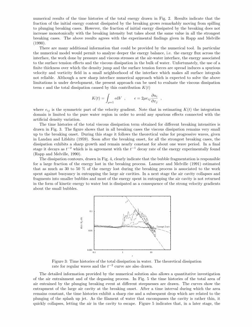
numerical results of the time histories of the total energy drawn in Fig. 2. Results indicate that thefraction of the initial energy content dissipated by the breaking grows remarkably moving from spillingto plunging breaking cases. However, the fraction of initial energy dissipated by the breaking does notincrease monotonically with the breaking intensity but takes about the same value in all the strongestbreaking cases. The above results agrees with the experimental findings given in Rapp and Melville(1990).

There are many additional information that could be provided by the numerical tool. In particularthe numerical model would permit to analyze deeper the energy balance, i.e. the energy flux across theinterface, the work done by pressure and viscous stresses at the air-water interface, the energy associatedto the surface tension effects and the viscous dissipation in the bulk of water. Unfortunately, the use of afinite thickness over which the density jump and the surface tension forces are spread induces a spuriousvelocity and vorticity field in a small neighborhood of the interface which makes all surface integralsnot reliable. Although a new sharp interface numerical approach which is expected to solve the abovelimitations is under development, the present approach can be used to evaluate the viscous dissipationterm ε and the total dissipation caused by this contribution K(t)

K(t) =∫

ρ=1

εdV , ε = 2µeij∂ui

∂xj,

where eij is the symmetric part of the velocity gradient. Note that in estimating K(t) the integrationdomain is limited to the pure water region in order to avoid any spurious effects connected with theartificial density variation.

The time histories of the total viscous dissipation term obtained for different breaking intensities isdrawn in Fig. 3. The figure shows that in all breaking cases the viscous dissipation remains very smallup to the breaking onset. During this stage it follows the theoretical value for progressive waves, givenin Landau and Lifshitz (1959). Soon after the breaking onset, for all the strongest breaking cases, thedissipation exhibits a sharp growth and remain nearly constant for about one wave period. In a finalstage it decays as t−2 which is in agreement with the t−1 decay rate of the energy experimentally found(Rapp and Melville, 1990).

The dissipation contours, drawn in Fig. 4, clearly indicate that the bubble fragmentation is responsiblefor a large fraction of the energy lost in the breaking process. Lamarre and Melville (1991) estimatedthat as much as 30 to 50 % of the energy lost during the breaking process is associated to the workspent against buoyancy in entrapping the large air cavities. In a next stage the air cavity collapses andfragments into smaller bubbles and most of the energy spent in entrapping the air cavity is not returnedin the form of kinetic energy to water but is dissipated as a consequence of the strong velocity gradientsabout the small bubbles.

0.001

0.01

0.1

0.1 1 10

K(t

) /

ET (

0)

t

t-2

2 γ exp(-2 γ t)

Figure 3: Time histories of the total dissipation in water. The theoretical dissipationrate for regular waves and the t−2 curve are also drawn.

The detailed information provided by the numerical solution also allows a quantitative investigationof the air entrainment and of the degassing process. In Fig. 5 the time histories of the total area ofair entrained by the plunging breaking event at different steepnesses are drawn. The curves show theentrapment of the large air cavity at the breaking onset. After a time interval during which the arearemains constant, the time histories exhibit a sharp rise and a subsequent drop which are related to theplunging of the splash up jet. As the filament of water that encompasses the cavity is rather thin, itquickly collapses, letting the air in the cavity to escape. Figure 5 indicates that, in a later stage, the

amount of air entrapped decays with time. From the analysis of the free–surface profiles, not shown here,it can be seen that bubbles gradually rise back towards the free–surface and eventually escape from thewater.

x

y

-0.4 -0.2 0 0.2 0.4 0.6-0.3

-0.2

-0.1

0

0.1

Figure 4: Dissipation contours in the pure water domain. The configuration is thatshown in the bottom picture of Fig. 1.

Although the above mechanism is the main responsible for the degassing of the air bubbles, a carefulanalysis has been conducted to estimate the role played by the numerical model on that regard. Dueto the numerical model adopted for the interface capturing, the model cannot describe closed contoursthickness of which is smaller than one grid cell, i.e. 0.6 millimeters in the present simulations. Moreover,because of the smooth density variation, bubbles or air filaments thinner than 2δP , which is about 3millimeters, cannot be considered fully resolved. In order to estimate which portion of the entrainedbubbles is resolved, an average thickness is evaluated as the ratio between the area of the bubble andthe maximum between the horizontal and vertical dimensions of the bubble. A bubble is consideredunresolved when the average thickness fails below 2δP .

0

0.005

0.01

0.015

0.02

0.025

0.03

0.035

0.04

0.045

0 2 4 6 8 10

A

t

Figure 5: Time histories of the total area of entrapped air bubbles.

0.498

0.5

0.502

0.504

0.506

0.508

0.51

0.512

0.514

0.516

0.518

0 2 4 6 8 10

Aw

t

0

0.0005

0.001

0.0015

0.002

0.0025

0.003

0.0035

0.004

0 2 4 6 8 10

As

t

Figure 6: On the left picture the total water area is drawn for ε = 0.6. On the rightpicture the time history of the total area of unresolved bubbles is shown.

The artificial degassing of thin air filaments or bubbles operated by the numerical scheme, can bequantitatively estimated from the total area occupied by water Aw, drawn in the left picture of Fig. 6for the case ε = 0.60. The comparison with the corresponding area of the unresolved bubbles given onthe right picture of Fig. 6, indicates that the sharpest increase in the water area occurs between t = 2.0and t = 4.0, during which the total area of the unresolved bubbles take the largest values. In total, at

the end of the numerical simulation, the artificial degassing can be estimated in about three per cent ofinitial water area.

6. ACKNOWLEDGMENTS

The work has been done in the framework of the Programma Ricerche INSEAN 2007-2009 financiallysupported by the Italian Ministero dei Trasporti.

7. REFERENCES

J.U. Brackbill, D.B. Kothe and C. Zemach, (1992) A continuum method for modeling surface tension, J.Comput. Phys., 100, 335–354.M. Brocchini and D.H. Peregrine (2001) The dynamics of strong turbulence at free surfaces. Part 1.Description, J. Fluid Mech., 449, 225–254.G. Chen, C. Kharif, S. Zaleski and J. Li (1999) Two-dimensional Navier–Stokes simulation of breakingwaves, Phys. Fluids, 11, 121–133.J. Grue, D. Clamond, M. Huseby and A. Jensen, (2003) Kinematics of extreme water waves, Eur. J.Mech. B Fluids, 25, 355–366.A. Iafrati and E.F. Campana, (2005) Free surface fluctuations behind microbreakers: space–time behaviorand subsurface flow field, J. Fluid Mech., 529, 311–347.A. Iafrati (2009) Numerical study of the effects of the breaking intensity on wave breaking flows, J. FluidMech., 622, 371–411.E. Lamarre and W.K. Melville (1991) Air entrainment and dissipation in breaking waves, Nature, 351,469–472.L.D. Landau and E.M. Lifshitz (1959) Fluid Mechanics, PergamonJ. Lighthill (1978) Waves in Fluids, Cambridge Univ.W.K. Melville, F. Veron and C.J. White (2002) The velocity field under breaking waves: coherent struc-tures and turbulence, J. Fluid Mech., 454, 203–233.H. Qiao and J.H. Duncan (2001) Gentle spilling breakers: crest flow-field evolution, J. Fluid Mech., 439,57–85.R.J. Rapp and W.K. Melville (1990) Laboratory measurements of deep-water breaking waves, Phil. Trans.R. Soc. Lond. A331, 735–800.H.A. van der Vorst (1992) Bi-CGSTAB: fast and smoothly converging variant of Bi-CG for the solutionof nonsymmetric linear systems, SIAM J. Sci. Stat. Comput., 13, 631–644.G.B. Whitham, (1974) Linear and nonlinear waves, Wiley InterscienceY. Zang, R.L. Street and J.R. Koseff (1994) A non-staggered grid, fractional step method for time-dependent incompressible Navier-Stokes equations in curvilinear coordinates, J. Comput. Phys, 114,18–33.

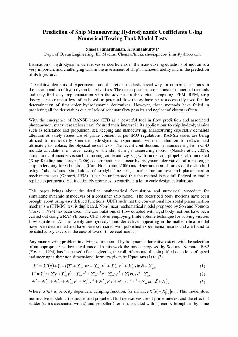
Prediction of Ship Manoeuvring Hydrodynamic Coefficients Using

Numerical Towing Tank Model Tests

Sheeja Janardhanan, Krishnankutty P Dept. of Ocean Engineering, IIT Madras, Chennai/India, sheejaphdoe_iitm@yahoo.co.in

Estimation of hydrodynamic derivatives or coefficients in the manoeuvring equations of motion is a

very important and challenging task in the assessment of ship’s manoeuvrability and in the prediction

of its trajectory.

The relative demerits of experimental and theoretical methods paved way for numerical methods in

the determination of hydrodynamic derivatives. The recent past has seen a host of numerical methods

and they find easy implementation with the advance in the digital computing. FEM, BEM, strip

theory etc. to name a few, often based on potential flow theory have been successfully used for the

determination of first order hydrodynamic derivatives. However, these methods have failed in

predicting all the derivatives due to lack of adequate flow physics and neglect of viscous effects.

With the emergence of RANSE based CFD as a powerful tool in flow prediction and associated

phenomenon, many researchers have focused their interest in its applications to ship hydrodynamics

such as resistance and propulsion, sea keeping and manoeuvring. Manoeuvring especially demands

attention as safety issues are of prime concern as per IMO regulations. RANSE codes are being

utilized to numerically simulate hydrodynamic experiments with an intention to reduce, and

ultimately to replace, the physical model tests. The recent contributions in manoeuvring from CFD

include calculations of forces acting on the ship during manoeuvring motion (Nonaka et-al, 2007),

simulations of manoeuvrs such as turning circle and zig-zag with rudder and propeller also modeled

(Xing-Kaeding and Jensen, 2006), determination of linear hydrodynamic derivatives of a passenger

ship undergoing forced motions (Cura-Hochbaum, 2006) and determination of forces on the ship hull

using finite volume simulations of straight line test, circular motion test and planar motion

mechanism tests (Ohmori, 1998). It can be understood that the method is not full-fledged to totally

replace experiments. Yet it definitely promises to contribute a lot to early design calculations.

This paper brings about the detailed mathematical formulation and numerical procedure for

simulating dynamic manoeuvrs of a container ship model. The prescribed body motions have been

brought about using user defined functions (UDF) such that the conventional horizontal planar motion

mechanism (HPMM) test is duplicated. Non-linear mathematical model proposed by Son and Nomoto

(Fossen, 1994) has been used. The computations of flow coupled with rigid body motions have been

carried out using a RANSE based CFD solver employing finite volume technique for solving viscous

flow equations. All the twenty one hydrodynamic derivatives appearing in the mathematical model

have been determined and have been compared with published experimental results and are found to

be satisfactory except in the case of two or three coefficients.

Any manoeuvring problem involving estimation of hydrodynamic derivatives starts with the selection

of an appropriate mathematical model. In this work the model proposed by Son and Nomoto, 1982

(Fossen, 1994) has been used after neglecting the roll effects and the simplified equations of speed

and steering in their non-dimensional form are given by Equations (1) to (3).

( ) ( ) extrrvvvr XXrXvXvrXTtuXX ′+′+′+′+′+′−+′=′ δδ sin1 22 (1)

extvrrvvrrrrvvvrv YYvrYrvYrYvYrYvYY ′+′+′+′+′+′+′+′=′ δδ cos2233 (2)

extvrrvvrrrrvvvrv NNvrNrvNrNvNrNvNN ′+′++′+′+′+′+′+′=′ δδ cos22233 (3)

Where ( )uX ′ is velocity dependent damping function, for instance ( ) uuXuXuu

′=′ . This model does

not involve modeling the rudder and propeller. Hull derivatives are of prime interest and the effect of

rudder (terms associated with δ) and propeller ( terms associated with t ) can be brought in by some

empirical relationships when required. Excitation forces from environment (terms associated with ext)

are neglected.

The formulation of the problem has in fact been tedious, as it involved a laborious procedure of many

trials to arrive at the expressions for body oscillations so that they in turn yield the most simplified

expressions for the calculation of hydrodynamic derivatives. Here the Fourier Series Expansion

method has been used for the determination of the derivatives according to which the hydrodynamic

forces and moments on the ship hull can be expressed as Hydrodynamic force/moment =

)sincos(3

0

tmbtma m

m

m ωω +∑=

where the Fourier constants are given by ∫=T

m tmtfT

a0

cos)(2

ω and ∫=T

m tmtfT

b0

sin)(2

ω

Fourier series expansion has been considered only up to third harmonic as the mathematical model

contains only up to third order terms. rvvuu ,,,, && and r& in Equations (1) to (3) have been substituted

with sinusoidal expressions while X ′ ,Y ′ and N ′ have been expanded in Fourier series as explained

above in three separate modes of motion viz. pure sway, pure yaw and combined sway and yaw

(mixed mode). Comparison of like terms in the corresponding equations has yielded the following

expressions for the hydrodynamic derivatives;

222

0

2xY

a

vv ay

Xω

= (4)

[ ]202

1xYxYuu

aaV

X −= (5)

12

0

1yY

a

v by

Yω

=&

(6)

333

0

4yY

a

vvv ay

Yω

−= (7)

[ ]13

0

31

yYyY

a

v aay

Y −=ω

(8)

12

0

1nN

a

v by

Nω

=&

(9)

333

0

4nY

a

vvv ay

Nω

−= (10)

[ ]13

0

31

nYnY

a

v aay

N −=ω

(11)

22

1xN

aN

u bu

X−

=&

(12)

−−= 22022

)(22

xNxYxY

aNcN

a

rr aaaV

uu

rX

(13)

1

1yN

a

r ar

Yω

=&

(14)

+

−= 3

2

3 4

4yN

axN

a

rrr brb

rY

ω

(15)

++−+= 3

22

14

3)2

(2

1yN

axNaN

cN

aN

axN

yN

a

r brbu

uu

rbb

rY

ωω

(16)

1

1nN

a

r ar

Nω

=&

(17)

33

4nN

a

rrr br

N−

=

(18)

[ ]31 31

nNnN

a

r bbr

N +=

(19)

aN

aYN

xN

a

yY

xYN

aaYN

vru

ub

y

bb

rvX 22

0

1

2

2−−=

ω

(20)

−

+−= 3

0232

14

4yN

aN

aYNxN

yYN

aaYN

vvr bu

urbb

rvY

ω

(21)

+

−=

3

332

4

a

aYN

yYyYN

aaYN

vrrv

vaa

rvY

(22)

[ ]332

4nNnYN

aaYN

vvr bbrv

N −=

(23)

+

−=

3

332

4

a

aYN

nYnYN

aaYN

vrrv

vaa

rvN

(24)

In the above equations subscript ‘a’ indicates amplitude of motion. Subscripts ‘Y’, ‘N’ and

‘YN’indicate pure sway, pure yaw and mixed modes respectively.

Simulation of HPMM requires a numerical computational domain and a solver capable of solving the

fluid flow equations while the mesh in the fluid domain re-orient with the hull motion. ICEM CFD

has been used for mesh generation and the dynamic mesh motion facility of the commercial CFD

package FLUENT has been made use of to bring about the prescribed motion of the ship body.

The size of the virtual towing tank used in the CFD modeling has been fixed as per ITTC guidelines

(ITTC quality manual, 1999) where the domain extends one ship length each from the port and

starboard, 0.8 ship length from the fore, 1.5 ship lengths form the aft and 0.64 ship length downwards

from the hull bottom. A 3-D unstructured grid with approximately 300,000 cells has been used for the

analysis. The block structured grid system has not been successful in producing oscillations in one

complete cycle due to the creation of negative volumes. Remeshing is required as the mesh on the

ship surface moves and this can be easily brought about by the solver in case of an unstructured grid

system than its structured counterpart. Meshing has been carried out in a number of trials such that it

is neither too coarse nor too fine and also uniformly graded through out the fluid domain.

A user defined function (UDF) has been written in C language using the macro

‘DEFINE_CG_MOTION’ and has been hooked into the main program in order to oscillate the mesh

on the hull surface. So, the solution process also consists of updating the mesh position at each time

step (0.005 sec, 20 iterations per time step). Free-surface effects have been neglected in the present

study. Flow velocity has been taken 1 m/sec and time period of oscillation 13.33 sec. Values for

motion velocity amplitudes were chosen such that they are neither too high nor too low. Many trials

have been carried out with various velocity amplitudes and the most feasible ones have been chosen.

Higher amplitudes caused mesh distortion and consequently dynamic mesh failure whereas lower

amplitudes have not been able to capture the non-linear part of the forces and moments. The

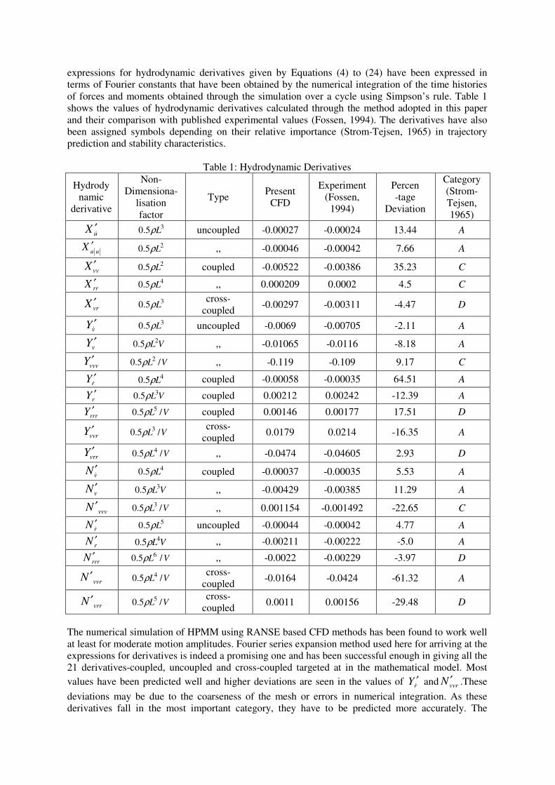
expressions for hydrodynamic derivatives given by Equations (4) to (24) have been expressed in

terms of Fourier constants that have been obtained by the numerical integration of the time histories

of forces and moments obtained through the simulation over a cycle using Simpson’s rule. Table 1

shows the values of hydrodynamic derivatives calculated through the method adopted in this paper

and their comparison with published experimental values (Fossen, 1994). The derivatives have also

been assigned symbols depending on their relative importance (Strom-Tejsen, 1965) in trajectory

prediction and stability characteristics.

Table 1: Hydrodynamic Derivatives

Hydrody

namic

derivative

Non-

Dimensiona-

lisation

factor

Type Present

CFD

Experiment

(Fossen,

1994)

Percen

-tage

Deviation

Category

(Strom-

Tejsen,

1965)

uX&′ 35.0 Lρ uncoupled -0.00027 -0.00024 13.44 A

uuX ′ 25.0 Lρ ,, -0.00046 -0.00042 7.66 A

vvX ′ 25.0 Lρ coupled -0.00522 -0.00386 35.23 C

rrX ′ 45.0 Lρ ,, 0.000209 0.0002 4.5 C

vrX ′ 35.0 Lρ cross-

coupled -0.00297 -0.00311 -4.47 D

vY&′ 35.0 Lρ uncoupled -0.0069 -0.00705 -2.11 A

vY ′ VL25.0 ρ ,, -0.01065 -0.0116 -8.18 A

vvvY ′ VL /5.0 2ρ ,, -0.119 -0.109 9.17 C

rY&′ 45.0 Lρ coupled -0.00058 -0.00035 64.51 A

rY ′ VL35.0 ρ coupled 0.00212 0.00242 -12.39 A

rrrY ′ VL /5.0 5ρ coupled 0.00146 0.00177 17.51 D

vvrY ′ VL /5.0 3ρ cross-

coupled 0.0179 0.0214 -16.35 A

vrrY ′ VL /5.0 4ρ ,, -0.0474 -0.04605 2.93 D

vN&′ 45.0 Lρ coupled -0.00037 -0.00035 5.53 A

vN ′ VL35.0 ρ ,, -0.00429 -0.00385 11.29 A

vvvN ′ VL /5.0 3ρ ,, 0.001154 -0.001492 -22.65 C

rN&′ 55.0 Lρ uncoupled -0.00044 -0.00042 4.77 A

rN ′ VL45.0 ρ ,, -0.00211 -0.00222 -5.0 A

rrrN ′ VL /5.0 6ρ ,, -0.0022 -0.00229 -3.97 D

vvrN ′ VL /5.0 4ρ cross-

coupled -0.0164 -0.0424 -61.32 A

vrrN ′ VL /5.0 5ρ cross-

coupled 0.0011 0.00156 -29.48 D

The numerical simulation of HPMM using RANSE based CFD methods has been found to work well

at least for moderate motion amplitudes. Fourier series expansion method used here for arriving at the

expressions for derivatives is indeed a promising one and has been successful enough in giving all the

21 derivatives-coupled, uncoupled and cross-coupled targeted at in the mathematical model. Most

values have been predicted well and higher deviations are seen in the values of rY&′ and vvrN ′ .These

deviations may be due to the coarseness of the mesh or errors in numerical integration. As these

derivatives fall in the most important category, they have to be predicted more accurately. The

research is still on for obtaining better values of derivatives. This work on the whole finds its success

in exploring and exploiting various features of a general purpose fluid flow solver to solve a non-

linear dynamic ship manoeuvring problem.

References

Cura-Hochbaum, A., Prediction of hydrodynamic coefficients for a passenger ship model, Int. Conf.

in Marine Hydrodynamics, pp. 933-942, 2006.

Fossen, T.I., Dynamics and stability of ships, Guidance and Control of Ocean Vehicles, John Wiley

and Sons, pp. 169-219, 1994.

ITTC Quality Manual, Uncertainty Analysis in CFD and Guidelines for RANS codes, 22nd

ITTC,

1999.

Nonaka, K., Miyazaki, H., Nimura, T., Ueno, M., Hino, T. and Kodama, Y., Calculation of

hydrodynamic forces acting on a ship in manoeuvring motion, Research Paper, Ship Research

Institute, Japan, pp. 307-317, 2007.

Ohmori, T., Finite-volume simulation of flows about a ship in maneuvering motion. Journal of Marine

Science and Technology, 3, pp. 82-93, 1998.

Strom-Tejsen, J., A Digital Computer Technique for the Prediction of Standard Manoeuvrs of Surface

Ships, DTRC Report 2130, 1965.

Xing-Kaeding, Y. and Jensen, A.G., Simulation of ship motions during manoeuvrs, Ship Technology

Research, vol.53(4), pp.14-28, 2006.

Nomenclature

ma Fourier constants associated with cosine terms

nNma Fourier constants associated with cosine terms of yaw equation in pure yaw mode

nYma Fourier constants associated with cosine terms of yaw equation in pure sway mode

nYNma Fourier constants associated with cosine terms of yaw equation in mixed mode

xNma Fourier constants associated with cosine terms of surge equation in pure yaw mode

xYma Fourier constants associated with cosine terms of surge equation in pure sway mode

xYNma Fourier constants associated with cosine terms of surge equation in mixed mode

yNma Fourier constants associated with cosine terms of sway equation in pure yaw mode

yYma Fourier constants associated with cosine terms of sway equation in pure sway mode

yYNma Fourier constants associated with cosine terms of sway equation in mixed mode

A Derivatives evaluated and deemed very important

mb Fourier constants associated with sine terms

nNmb Fourier constants associated with sine terms of yaw equation in pure yaw mode

nYmb Fourier constants associated with sine terms of yaw equation in pure sway mode

nYNmb Fourier constants associated with sine terms of yaw equation in mixed mode

xNmb Fourier constants associated with sine terms of surge equation in pure yaw mode

xYmb Fourier constants associated with sine terms of surge equation in pure sway mode

xYNmb Fourier constants associated with sine terms of surge equation in mixed mode

yNmb Fourier constants associated with sine terms of sway equation in pure yaw mode

yYmb Fourier constants associated with sine terms of sway equation in pure sway mode

yYNmb Fourier constants associated with sine terms of sway equation in mixed mode

C Derivatives evaluated and deemed of minor importance

D Derivatives evaluated and deemed negligible

L Length between perpendiculars of the vessel

m Integer for determining harmonics of Fourier series

N ′ Non-dimensional hydrodynamic reaction moment in yaw

rr &,

Yaw rate, yaw acceleration of the model

T Period of oscillation

uu &,

Surge velocity, surge acceleration of the model

vv &,

Sway velocity, sway acceleration of the model

V Forward velocity of the vessel

X ′ Non-dimensional hydrodynamic reaction force in surge

Y ′ Non-dimensional hydrodynamic reaction force in sway

N ′

Non-dimensional hydrodynamic moment in yaw

γ Arbitrary value of phase which depends on the start value of oscillation

ω Circular frequency of oscillation

Numerical optimisation of resistance and wake quality for a VLCC

Martin Kjellberg (martin.kjellberg@chalmers.se)†, Carl-Erik Janson (janson@flowtech.se)‡

†Dept. of Shipping and marine technology, Chalmers University of Technology, SE-412 96, Göteborg, Sweden ‡FLOWTECH International, PO Box 24001, SE-400 22, Göteborg, Sweden

1 Introduction Formal optimisation of hull forms using computational fluid dynamics (CFD) is nothing new and has for example been applied successfully on bulbs and forebodies using potential flow codes [1]. While proving efficient for forebody optimisation of wave resistance, the highly viscous flow around the afterbody and especially the wake cannot be captured by potential flow methods. Reynolds-averaged Navier-Stokes (RANS) methods are now able to predict not only the resistance accurately but also the wake flow is predicted well enough to be used properly in formal afterbody optimisations. The computational effort required in such a task can quite easily become unfeasible and the potential of a successful outcome of the optimisation needs to be balanced with the ability and generality of the hull deformation scheme as well as with the size and density of the grid, simply to keep the computational effort down.

This paper presents the work done on numerical stern shape optimisations based on the computed viscous flow using CFD. The majority of the effort was carried out within Virtual Tank Utility in Europe (VIRTUE), an EU 6th Framework Programme funded project, together with partners from the industry and academia. The focus of this paper will, however, be on the work carried out at Chalmers.

After initial sensitivity studies and validation of the CFD codes on three different hulls, two optimisation rounds were carried out, enabling the second to make use of the knowledge gained from the first round. The part of the work presented here will focus on the results of the initial validation studies and the second optimisation round.

2 Numerical method The computations were performed using the zonal approach [2] in the CFD software SHIPFLOW and involves three different methods. A potential flow method [3] computes the inviscid flow and provides input for a boundary layer method [2] used on the forward half of the hull. A RANS code [4] is used to predict the viscous flow aft of mid ship and the solutions from the potential flow method and the boundary layer method are used as boundary condition for the viscous domain.

The advantage of this approach is reduced computational effort while sacrificing the possibility to capture viscous effects in the forward half of the hull, like bilge vortices. It is assumed, however, that these effects are small.

Grid dependence and different turbulence models were investigated in the early stages and finally a grid size of 205x70x100 cells, a y+-value of 0.7 and for closure, the explicit algebraic stress model (EASM) [4] were used in the second optimisation round. This grid is somewhat denser than normal in the longitudinal direction and the additional cells were placed close to the propeller plane to increase the resolution of the flow affecting the wake as well as to enhance the staircase approximation of the stern profile because of the H-O grid.

3 Validation of the flow computations A total of four different hulls were used for validation of the flow computations. Three of the validations were conducted before the optimisation exercise started and one was conducted afterwards. The first two hulls, KVLCC1 and KVLCC2, as seen in Figure 1(a), have the same forebodies but slightly different afterbodies and were used to validate correct ranking [5]. The third hull, VIRTUE Initial Tanker, was later was used as the initial hull form in the optimisation, see Figure 1(b). After the second optimisation round all partners supplied one candidate hull and the candidate that seemed most promising, provided by MARIN, was selected as the VIRTUE Optimised Tanker. A model was built and tested also for this hull.

Two objective functions were defined and used in the optimisation, the total double-model viscous resistance Cvt and a wake objective function WOF that considers the variation of velocities along five different radii in the propeller disk as well as the nominal wake in the same region.

(a) (b) Figure 1 (a) Body plan of KVLCC1 (dotted) and KVLCC2 (solid.). (b) Body plan of VIRTUE Initial Tanker

The results from the initial study are presented in Table 1 and 2. The computations of KVLCC1 and KVLCC2 were underpredicting the resistance and overpredicting the wake objective function. While the absolute values are not perfect, especially for the wake objective function, the ranking is correct and differences in objective functions between the hulls compared to measurements must be considered to be very good. This is something that is very important for the optimisation process to work properly. The agreement of computed and experimental values is better for the VIRTUE hulls.

Table 1 Comparison of objective function values 1000Cvt WOF KVLCC1 3.883 (-3.65%) 0.464 (+20.52%) KVLCC1 exp. 4.030 0.385 KVLCC2 3.943 (-2.88%) 0.369 (+27.24%) KVLCC2 exp. 4.060 0.290 VIRTUE Initial Tanker 3.894 (+1.41%) 0.221 (-11.95%) VIRTUE Initial Tanker exp. 3.840 0.251 VIRTUE Optimised Tanker 3.770 (+1.59%) 0.260 (-7.14%) VIRTUE Optimised Tanker exp. 3.711 0.280 Table 2 Comparison of the differences in objective function values for KVLCC2 / KVLCC1 and VIRTUE Optimised Tanker / VIRTUE Initial Tanker

KVLCC2 / KVLCC1 VIRTUE Optimised Tanker / VIRTUE Initial Tanker

Δ1000Cvt 0.060 (+1.55%) -0.124 (-3.18%) Δ1000Cvt exp. 0.030 (+0.74%) -0.129 (-3.36%) ΔWOF -0.095 (-20.47%) 0.039 (+17.65%) ΔWOF exp. -0.095 (-24.68%) 0.029 (+11.55%)

Considering the flow field, Figure 2(a) and (b) further shows good agreement with the experiments if comparing the differences in the characteristics of the wake. Locally, larger differences in the contours, i.e. absolute values, can be seen.

The characteristics of the wake are captured well for the VIRTUE Initial Hull and VIRTUE Optimised Hull as well which can be seen in Figure 2(c) and (d). The tendencies of a somewhat less pronounced island in the hook appear also in these cases.

(a) (b)

(c) (d)

Figure 2 (a) Computed and (b) measured wake for KVLCC1 and KVLCC2, (c) computed and measured wake for VIRTUE Initial Hull, (d) computed and measured wake for VIRTUE Optimised Hull.

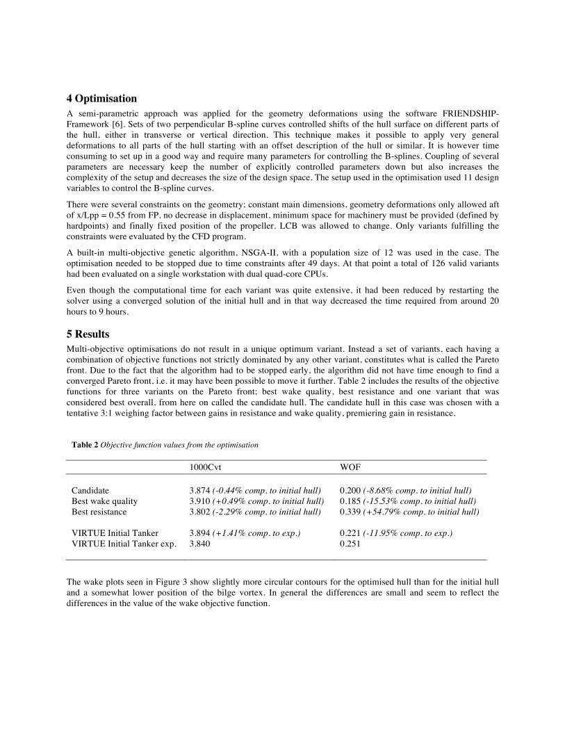
4 Optimisation A semi-parametric approach was applied for the geometry deformations using the software FRIENDSHIP-Framework [6]. Sets of two perpendicular B-spline curves controlled shifts of the hull surface on different parts of the hull, either in transverse or vertical direction. This technique makes it possible to apply very general deformations to all parts of the hull starting with an offset description of the hull or similar. It is however time consuming to set up in a good way and require many parameters for controlling the B-splines. Coupling of several parameters are necessary keep the number of explicitly controlled parameters down but also increases the complexity of the setup and decreases the size of the design space. The setup used in the optimisation used 11 design variables to control the B-spline curves.

There were several constraints on the geometry; constant main dimensions, geometry deformations only allowed aft of x/Lpp = 0.55 from FP, no decrease in displacement, minimum space for machinery must be provided (defined by hardpoints) and finally fixed position of the propeller. LCB was allowed to change. Only variants fulfilling the constraints were evaluated by the CFD program.

A built-in multi-objective genetic algorithm, NSGA-II, with a population size of 12 was used in the case. The optimisation needed to be stopped due to time constraints after 49 days. At that point a total of 126 valid variants had been evaluated on a single workstation with dual quad-core CPUs.

Even though the computational time for each variant was quite extensive, it had been reduced by restarting the solver using a converged solution of the initial hull and in that way decreased the time required from around 20 hours to 9 hours.

5 Results Multi-objective optimisations do not result in a unique optimum variant. Instead a set of variants, each having a combination of objective functions not strictly dominated by any other variant, constitutes what is called the Pareto front. Due to the fact that the algorithm had to be stopped early, the algorithm did not have time enough to find a converged Pareto front, i.e. it may have been possible to move it further. Table 2 includes the results of the objective functions for three variants on the Pareto front; best wake quality, best resistance and one variant that was considered best overall, from here on called the candidate hull. The candidate hull in this case was chosen with a tentative 3:1 weighing factor between gains in resistance and wake quality, premiering gain in resistance.

Table 2 Objective function values from the optimisation 1000Cvt WOF Candidate 3.874 (-0.44% comp. to initial hull) 0.200 (-8.68% comp. to initial hull) Best wake quality 3.910 (+0.49% comp. to initial hull) 0.185 (-15.53% comp. to initial hull) Best resistance 3.802 (-2.29% comp. to initial hull) 0.339 (+54.79% comp. to initial hull) VIRTUE Initial Tanker 3.894 (+1.41% comp. to exp.) 0.221 (-11.95% comp. to exp.) VIRTUE Initial Tanker exp. 3.840 0.251

The wake plots seen in Figure 3 show slightly more circular contours for the optimised hull than for the initial hull and a somewhat lower position of the bilge vortex. In general the differences are small and seem to reflect the differences in the value of the wake objective function.

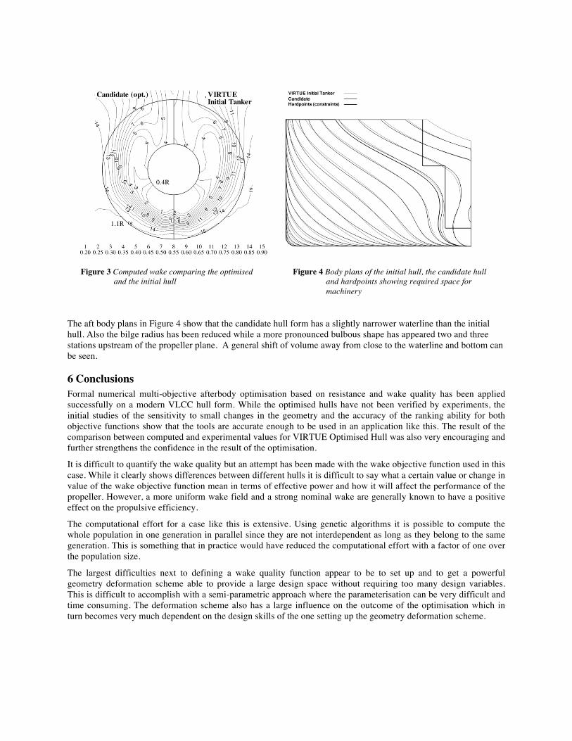
Figure 3 Computed wake comparing the optimised Figure 4 Body plans of the initial hull, the candidate hull

and the initial hull and hardpoints showing required space for machinery

The aft body plans in Figure 4 show that the candidate hull form has a slightly narrower waterline than the initial hull. Also the bilge radius has been reduced while a more pronounced bulbous shape has appeared two and three stations upstream of the propeller plane. A general shift of volume away from close to the waterline and bottom can be seen.

6 Conclusions Formal numerical multi-objective afterbody optimisation based on resistance and wake quality has been applied successfully on a modern VLCC hull form. While the optimised hulls have not been verified by experiments, the initial studies of the sensitivity to small changes in the geometry and the accuracy of the ranking ability for both objective functions show that the tools are accurate enough to be used in an application like this. The result of the comparison between computed and experimental values for VIRTUE Optimised Hull was also very encouraging and further strengthens the confidence in the result of the optimisation.

It is difficult to quantify the wake quality but an attempt has been made with the wake objective function used in this case. While it clearly shows differences between different hulls it is difficult to say what a certain value or change in value of the wake objective function mean in terms of effective power and how it will affect the performance of the propeller. However, a more uniform wake field and a strong nominal wake are generally known to have a positive effect on the propulsive efficiency.

The computational effort for a case like this is extensive. Using genetic algorithms it is possible to compute the whole population in one generation in parallel since they are not interdependent as long as they belong to the same generation. This is something that in practice would have reduced the computational effort with a factor of one over the population size.

The largest difficulties next to defining a wake quality function appear to be to set up and to get a powerful geometry deformation scheme able to provide a large design space without requiring too many design variables. This is difficult to accomplish with a semi-parametric approach where the parameterisation can be very difficult and time consuming. The deformation scheme also has a large influence on the outcome of the optimisation which in turn becomes very much dependent on the design skills of the one setting up the geometry deformation scheme.

7 References [1] Valdenazzi F., Harries S., Janson C.-E., Leer-Andersen M., Maisonneuve J.-J., Marzi J., Raven H.: The FANTASTIC RoRo: CFD Optimisation of the Forebody and its Experimental Verification, International Conference on Ship and Shipping Research (NAV 2003), Palermo, 2003

[2] Larsson L., Broberg L., Kim K.-J. & Zhang D.-H.: A method for resistance and flow prediction in ship design. SNAME Annual Meeting, 1990

[3] Janson C.-E.: Potential Flow Panel Methods for the Calculation of Free-surface Flows with Lift, PhD thesis, Department of shipping and marine technology, Chalmers, Göteborg, 1997.

[4] Flowtech International AB, XCHAP – theoretical manual, 2007

[5] Kim W.-J., Kim D.-H., Van S.-H.: Computational study on turbulent flows around modern tanker hull forms, Int. J. Numer. Meth. Fluids, 38 (2002) 377-406, John Wiley & Sons, Ltd.

[6] Abt C., Harries S.: A New Approach to Integration of CAD and CFD for Naval Architects, 6th International Conference on Computer Applications and Information Technology in the Maritime Industries (COMPIT2007), Cortona, 2007

Validation of the RANSE Rigid Body Motion Computations

Marek Kraskowski, Ship Design and Research Centre S.A., Poland marek.kraskowski@cto.gda.pl

The following paper is the continuation of the paper presented at NuTTS’08 in Brest, which concerning the application of the rigid body motion module and wavemaker module for COMET solver, elaborated by Ship Design and Research Centre S.A. The previous paper contained the mathematical formulation of the rigid body motion problem, as well as the description of boundary conditions for the simulation of wave motion. Two examples of application were also presented – a free drop of the cube, and the motion of the megayacht in regular head waves. However, no validation was presented; the correctness of the computations was assessed only qualitatively by visual control of the behaviour of the objects. In the present paper, experimental validation of the free drop simulation is presented, as well as the validation of the simulation of the hull motion in waves, based on the strip theory results.

The principles of the free drop test case are briefly summarized here: – A cube of 0.15m x 0.15 m x 0.15 m is dropped freely into calm water. – The initial conditions are as follows: the cube hangs freely by one corner, the opposite corner is

located 50 mm above the water surface (Fig.1). – The mass distribution of the cube is asymmetrical, and the initial position of the cube is set so as

to enforce capsizing of the cube after falling into the water. – The mass of the cube is 1.81 kg, so in case of free floating in calm water, approximately half of

the volume is submerged.

Fig. 1 Free drop test case.

The experiment was designed so as to be possibly cheap and informative – the motion of the cube after releasing was only recorded with the high speed video camera at 125 frames per second. The glass tank of 1m x 1.3m was used, the water depth was set at 0.25m. In order to check whether the behaviour of the cube is not random, the experiment was repeated for few times and the motion was recorded from two directions, differing by 90 degrees. Frame-by-frame comparing of the videos revealed sufficient coincidence. The CFD simulation was carried out after preparing the cube for the test, so as to assure that the mass properties of it are set accurately. Details of the numerical simulation setup were as follows: − The o-type hexahedral mesh was generated in the spherical domain around the cube, containing

1750000 cells. − The static pressure boundary condition was applied at the outer surface of the domain.

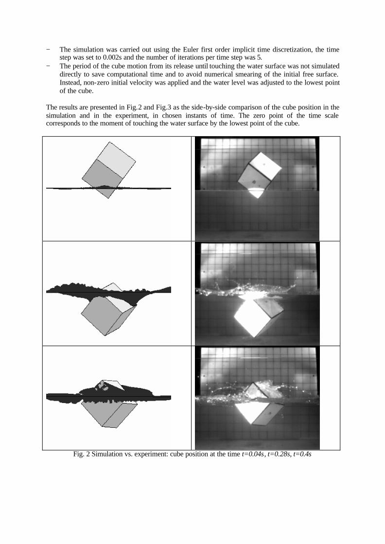
− The simulation was carried out using the Euler first order implicit time discretization, the time step was set to 0.002s and the number of iterations per time step was 5.

− The period of the cube motion from its release until touching the water surface was not simulated directly to save computational time and to avoid numerical smearing of the initial free surface. Instead, non-zero initial velocity was applied and the water level was adjusted to the lowest point of the cube.

The results are presented in Fig.2 and Fig.3 as the side-by-side comparison of the cube position in the simulation and in the experiment, in chosen instants of time. The zero point of the time scale corresponds to the moment of touching the water surface by the lowest point of the cube.

Fig. 2 Simulation vs. experiment: cube position at the time t=0.04s, t=0.28s, t=0.4s

Fig. 3 Simulation vs. experiment: cube position at the time t=0.48s, t=0.60s, t=0.72s

Satisfactory results of the experimental validation of the 6DOF module confirm the correctness of the mathematical model and the coding of the programs. After t=1s, approximately, the results of the simulation and the experiment are no longer in as good conformity due to the influence of reflected waves, which are not captured by the numerical model. The case of free drop is relatively simple in fact, due to short time of simulation, no constraints of the motion and low influence of the numerical noise. Final goal of the work is to elaborate the complete tool and method for simulating the hull motion in waves, and the attempt on such simulation for a container ship hull is presented here. The following assumptions were done for the simulation of the hull motion in waves: − Only head waves were considered. The problem was then limited to two degrees of freedom, the

rest of them was simply locked. The problem of numerical diffusion of the waves in case when

the wave direction is not parallel to the mesh lines is also avoided, which makes the problem much simpler than the simulation for arbitrary wave direction.

− The approach to moving mesh problem for rigid body motion simulation is based on the one proposed by Azcueta (2001) – entire mesh is moving together with the hull. An advantage of such approach is its simplicity, a disadvantage – problem with mass conservation and preserving the wave parameters when the entire domain is moving violently.

− Only regular waves were considered. Computation of the ship response in the frequency domain for irregular waves would require extremely long computational time.

The test case vessel was a container ship of LPP=160m with bulbous bow, sailing at 19 knots. In order to reduce the computational time, the simulation was carried out at model scale 1:30. Generation of the waves in the computational domain is realized by the “two-inlet” approach proposed by Wöckner et al (2007) – unsteady velocity field computed on the basis of linear wave theory is prescribed both at inlet and outlet of the domain, the hydrostatic pressure is applied on top and bottom on the domain. The simulation was carried out for one speed of the vessel and a range of wave periods. The parameters of waves considered in the simulation are listed in table below.

No. Wave amplitude [m] Wave period [s] Wave length [m] 1 1.25 8 100 2 1.25 10 156 3 1.25 14 306 4 1.25 20 625

The computational mesh parameters are extremely important for the RANSE simulation of waves so the list of the mesh features is given here: − The flow was computed in rectangular domain, with the boundaries located 1.25 LPP upstream

from the fore perpendicular, 1.25 LPP downstream from the aft perpendicular, 1.25 LPP to the side from the symmetry plane and 0.6 LPP below the baseline of the hull.

− The mesh of hexahedral, block-structured type was used, consisting of app. 1 000 000 cells. − Maximum cell length in the flow direction was 0.054 of the shortest wave length. − The height of the cells in the region where the free surface was present ranged from 0.06 to 0.09

of the wave height. The mesh density on the fore part of the hull surface is presented in Fig.4.

Fig. 4 Mesh details in the bow region

Three values of time step were tested in order to check its influence on the simulation stability and parameters of the hull motion. The values of them were: dt=0.003s, dt=0.005s and dt=0.0075s. Influence of the time step on the simulation results is presented in Fig.5: the vertical acceleration at fore perpendicular is plotted versus time, for all considered values of the time step. It can be seen that increasing the time step value reduces the noise (smoother curve), but also reduces the extreme values of the acceleration. The largest value of the time step should be then avoided due to considerable damping of the hull motion. On the other hand, smallest value of the time step leads to high noise,

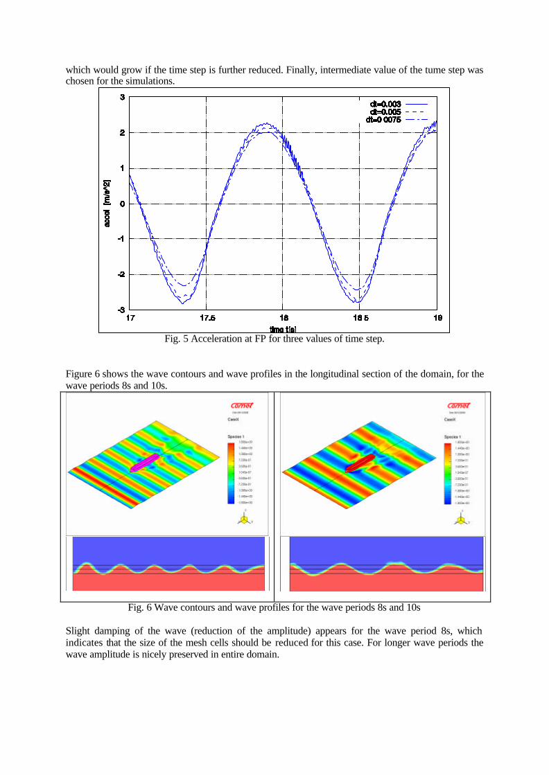
which would grow if the time step is further reduced. Finally, intermediate value of the tume step was chosen for the simulations.

Fig. 5 Acceleration at FP for three values of time step.

Figure 6 shows the wave contours and wave profiles in the longitudinal section of the domain, for the wave periods 8s and 10s.

Fig. 6 Wave contours and wave profiles for the wave periods 8s and 10s Slight damping of the wave (reduction of the amplitude) appears for the wave period 8s, which indicates that the size of the mesh cells should be reduced for this case. For longer wave periods the wave amplitude is nicely preserved in entire domain.

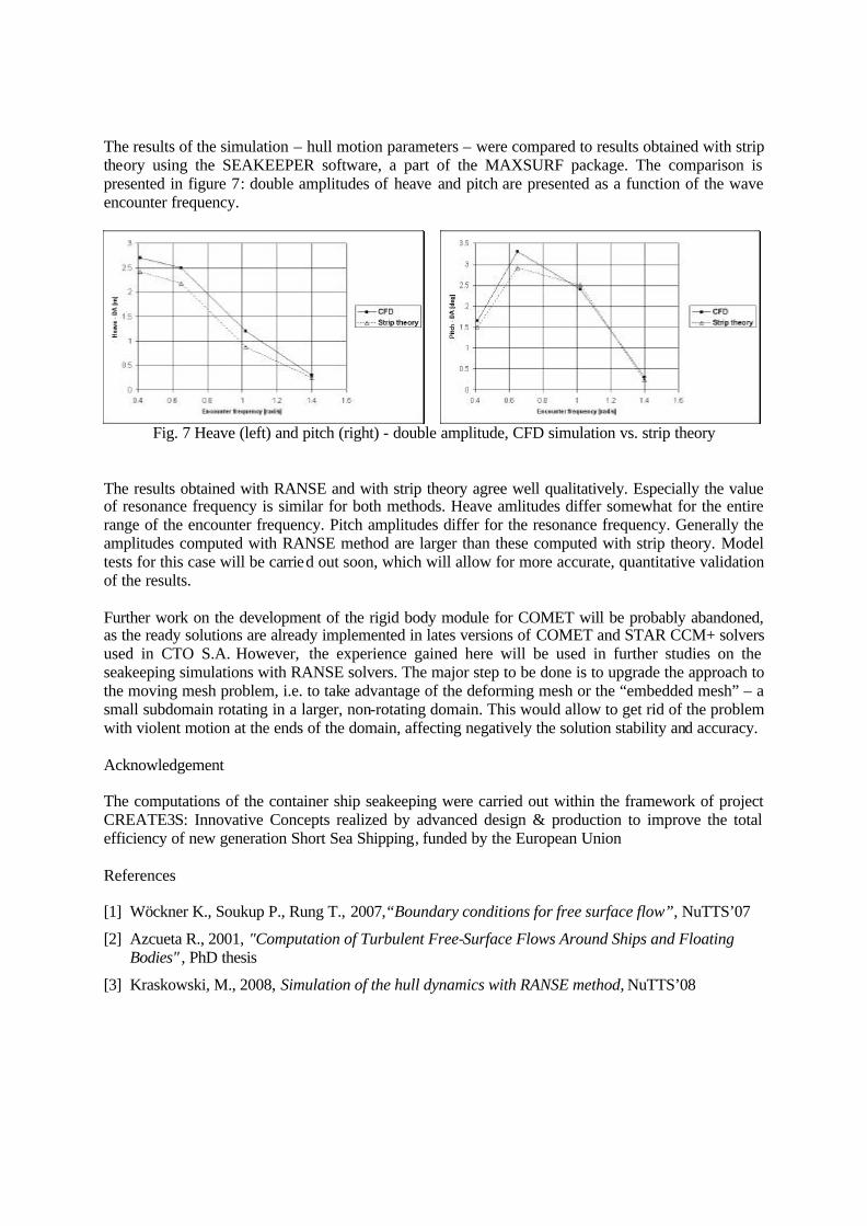
The results of the simulation – hull motion parameters – were compared to results obtained with strip theory using the SEAKEEPER software, a part of the MAXSURF package. The comparison is presented in figure 7: double amplitudes of heave and pitch are presented as a function of the wave encounter frequency.

Fig. 7 Heave (left) and pitch (right) - double amplitude, CFD simulation vs. strip theory

The results obtained with RANSE and with strip theory agree well qualitatively. Especially the value of resonance frequency is similar for both methods. Heave amlitudes differ somewhat for the entire range of the encounter frequency. Pitch amplitudes differ for the resonance frequency. Generally the amplitudes computed with RANSE method are larger than these computed with strip theory. Model tests for this case will be carried out soon, which will allow for more accurate, quantitative validation of the results. Further work on the development of the rigid body module for COMET will be probably abandoned, as the ready solutions are already implemented in lates versions of COMET and STAR CCM+ solvers used in CTO S.A. However, the experience gained here will be used in further studies on the seakeeping simulations with RANSE solvers. The major step to be done is to upgrade the approach to the moving mesh problem, i.e. to take advantage of the deforming mesh or the “embedded mesh” – a small subdomain rotating in a larger, non-rotating domain. This would allow to get rid of the problem with violent motion at the ends of the domain, affecting negatively the solution stability and accuracy. Acknowledgement The computations of the container ship seakeeping were carried out within the framework of project CREATE3S: Innovative Concepts realized by advanced design & production to improve the total efficiency of new generation Short Sea Shipping, funded by the European Union References [1] Wöckner K., Soukup P., Rung T., 2007,“Boundary conditions for free surface flow”, NuTTS’07

[2] Azcueta R., 2001, "Computation of Turbulent Free-Surface Flows Around Ships and Floating Bodies" , PhD thesis

[3] Kraskowski, M., 2008, Simulation of the hull dynamics with RANSE method, NuTTS’08

New algorithms to speed up RANSE computations in hydrodynamicsAlban Leroyer, Patrick Queutey, Emmanuel Guilmineau, Ganbo Deng and Michel Visonneau

Laboratoire de Mecanique des Fluides, Ecole Centrale de NantesUMR-CNRS 6598, 44321 Nantes Cedex 3, France

Alban.Leroyer@ec-nantes.fr

1 Introduction

Free-surface capturing methods (volume of fluid, level-set formulation) have become more and morepopular among the CFD developers involved in viscous naval hydrodynamics. This increasing interest isdue to the fact that this approach is more robust than those based on a free-surface fitting methodologysince no regridding is necessary. Moreover, the merging or breakup of the interface is also handled in anatural way. To achieve such computations, specific compressive discretisation schemes are used to solvethe concentration transport equation and keep the sharpness of the interface [1, 2]. Even if the capacitiesand the flexibility of such an approach is unquestionable, two features (easily assimilated as drawbacks)can be highlighted :

– the formulation is intrinsically unsteady since the concentration is convected by the flow. Up tonow, any steady formulation has ever been successful, to the knowledge of the authors,

– the compressive property has numerically severe Courant number limitation.

So, this is quite wastefulness to use such an approach when dealing with physical steady cases. It isall the more a pity since for an implicit solver, the concentration equation is the sore equation to havesuch a Courant number limitation ! This issue was first underlined by Ubbink in the conclusions of hisPhD thesis [1] : « the Courant limitation is not insurmountable because it should be possible to apply atechnique of sub-cycling where the time step of the main loop is divided into smaller steps in order toadvect the volume fractions... ».

Therefore, to reduce this Courant number limitation, such an original time-splitting (which can alsobe noted time sub-cycling) procedure for the concentration equation has been successfully developed andvalidated for steady state cases. For instance, it enables to increase the global time step while keepingthe Courant number constant. It raises no problem for fixed bodies. However, when using the Newton’slaw for solved motions, the large time steps lead to a divergent flow/motion coupling, due to the addedmass effects. To avoid this problem, a quasi-static approach has been developed to reach an equilibriumposition. The latter has been successfully combined with the time-splitting procedure for the concentra-tion without problems of stability. Compared to a classical unsteady approach using the Newtow’s law,this new numerical procedure to deal with steady cases for hydrodynamics applications enables to reducesignificantly the CPU time.

After a brief description of the RANSE solver in which this work has been implemented, this articleoutlines the time-splitting procedure as well as the quasi-static approach. Then, a test-case is shown,demonstating the capability and the efficiency of these techniques.

2 The ISIS-CFD flow solver

ISIS-CFD, available as a part of the FINETM/Marine computing suite, is an incompressible unsteadyReynolds-Averaged Navier-Stokes (RANSE) solver. It is developed by the EMN group (Equipe Modeli-sation Numerique) of the Fluid Mechanics Laboratory of the Ecole Centrale Nantes. The solver is basedon a Finite-Volume method to build a second-order accurate discretisation of the RANS equations. Theface-based method is generalised to unstructured meshes for which non-overlapping control volumes arebounded by an arbitrary number of constitutive faces. It enables to deal with complex geometries. Thevelocity field is obtained from the momentum conservation equations and the pressure field is extractedfrom the mass conservation constraint, or continuity equation, transformed into a pressure equation. Inthe case of turbulent flows, additional transport equations for modeled variables are solved in a formsimilar to the momentum equations : they are discretised and solved using the same principles.

Free-surface flows are computed through an interface capturing method : the flow phases are mo-delled through the use of a transport equation for the volume fraction (or concentration) of water cw ineach cell : cw = 1 means that the cell is completely filled with water, cw = 0 means that only air ispresent in the considered cell. The interface between air and water is defined by the surface cw = 0.5.The effective flow physical properties (dynamic viscosity µ and density ρ) are obtained from each phaseproperties, (µw,µa) and (ρw,ρa), respectively for water and air, with the following constitutive relations :µ = cwµw + (1− cw)µa and ρ = cwρw + (1− cw)ρa.

Special attention has to be paid to preserve the sharpness of the interface when solving the transportequation of cw. This equation is then discretised with a specific compressive scheme, including a Courantnumber limitation to ensure a limited diffusion of the interface (the Courant number is an adimensionalparameter roughly defined by : ∆t V/∆x , where V is the velocity through the considered cell, ∆x thesize of the cell, and ∆t the global time-step of the temporal discretisation). As a result, the discretisedtime-step has to be small enough to fulfil this CFL condition and thus ensure the compressive properties[2].

An ALE (Arbitrary Lagrangian Eulerian) approach is used to deal with moving bodies. All configu-rations of motion (up to 6 solved or imposed DOF) can be applied. Ad-hoc deformation techniques havethus been developed to keep a body-fitted mesh during its motion [3, 4].

3 The time-splitting procedure for concentration

3.1 Description

With an interface capturing approach, we have to solve Eq. (1), (cw is simply denoted by c in thefollowing) :

δ

δt

∫Vc dV +

∮Sc(−→U −−→Ud)·−→n dS = 0 , (1)

where V is the domain of interest, or control volume, bounded by the closed surface S moving at thevelocity

−→U d with a unit normal vector −→n directed outward. The time derivative following the moving

grid is written δ /δt.

The classical discretization leads therefore to the following discretized form :

c(tc)V (tc)− c(tp)V (tp)∆t

+∑

facesSf

cf

(F−→

U−F−→

Ud

)= 0 (2)

where tp and tc mean respectively the previous and the current time, and ∆t = tc − tp the current timestep. cf denotes the reconstruction of the fraction volume at the centre of the face, whereas F−→

Uand F−→

Udrepresent respectively the velocity flux and the grid displacement velocity flux through the consideredface Sf .Since steady configurations are investigated here, the basic first order Euler implicit scheme is appliedfor the time derivative.

The spirit of the time-splitting approach is to reduce the CFL condition related to Eq. (2), by using aspecific time step for the fraction volume, which is a multiple of the time step associated with the globalsimulation. In other terms, the global time step ∆t is splitted into a sequence of smaller ones leadingnaturally to smaller Courant numbers. As a consequence, the volume fraction equation (3) is solvedsequentially several times during a single global time step, sometimes denoted « subcycles ». If we noteNthe number of « subcycles », the splitted time step ∆ti is then equal to ∆t/N . The intermediate volumesV i, which do not correspond to physical configurations of the mesh, are simply linearly interpolatedbetween tp and tc.

ci V i − ci−1 V i−1

∆ti+

∑facesSf

cif

(F−→

U−F−→

Ud

)= 0 (3)

Figure 1: Temporal diagram

Instead of solving Eq. (2), we solve N times Eq. (3), going forward in time progressively. From oneequation with a typical Courant Number Co for the classical approach, the time-splitting approach leadstoN equations to solve but with typical Courant numbers around Co/N . Finally, by suming Eq. (3) fromi equal 1 to N , we obtain the following form Eq. (4) similar to Eq. (2).

c(tc)V (tc)− c(tp)V (tp)∆t

+∑

facesSf

cf

(F−→

U−F−→

Ud

)= 0 ,with cf =

N∑i=1

cifN

(4)

The free-surface moves then little by little during theses small time steps. As the CPU time related to theresolution of the volume fraction equation is not large compared with other parts of the solver (especiallycompared to the resolution of the pressure), the global CPU time of the simulation is strongly reduced.When the steady state of the flow is reached, the solution is obviously the same as those obtained with aclassical approach, since the temporal derivative term is vanished. Then, solving once or several times anequation of convection with a null temporal derivative does not change anything. With the approach, theway to reach the steady case remain quite physical (even if we try to remove the transitory state quicklywithout solving it accurately). It seems to be the reason why this procedure is very robust.

3.2 ExampleTo illustrate this procedure, a 2-D configuration of a submerged NACA-0012 hydrofoil is considered.

This well-known test-case, experimentally investigated by Duncan [5] is often used for the validation ofnumerical method developed to compute free-surface flows. In the experimental setup, the hydrofoil,whose chord is c = 20.3 cm, is towed in a tank with speed U∞ = 0.8 m/s with an angle of attack α = 5˚(see Fig. 2). The relevant non-dimensional parameters based on the chord length and the free-streamvelocity are Fr = 0.5672 and Re = 1.423e5. The distance between the profile and the bottom of thebasin is kept fixed (H = 17.5 cm from the mid-chord of the profile), whereas the depth of submergences is varying. Here, we only interest in the case s = 23.6 cm.

Figure 2: Experimental setup Figure 3: View of the mesh

The simulations have been performed using a mesh of 38000 cells (Fig. 3). Here, the two-equationk − ω SST closure [6] was used to take into account the turbulence phenomena. Boundary conditionsare imposed as follows : on the top and on the outlet, an hydrostatic pressure is imposed. On the inlet,velocity is imposed with its far field value. A slip condition is applied on the bottom of the tank, whereaswall-function boundaries are attached to the whole surface of the foil.

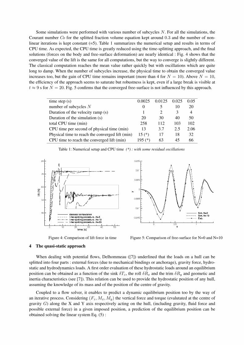
Some simulations were performed with various number of subcycles N . For all the simulations, theCourant number Co for the splitted fraction volume equation kept around 0.3 and the number of non-linear iterations is kept constant (=5). Table 1 summarizes the numerical setup and results in terms ofCPU time. As expected, the CPU time is greatly reduced using the time-splitting approach, and the finalsolutions (forces on the body and free-surface deformation) are nearly identical : Fig. 4 shows that theconverged value of the lift is the same for all computations, but the way to converge is slightly different.The classical computation reaches the mean value rather quickly but with oscillations which are quitelong to damp. When the number of subcycles increase, the physical time to obtain the converged valueincreases too, but the gain of CPU time remains important (more than 4 for N = 10). Above N = 10,the efficiency of the approach seems to saturate but robustness is kept, even if a large break is visible att ≈ 9 s for N = 20. Fig. 5 confirms that the converged free-surface is not influenced by this approach.

time step (s) 0.0025 0.0125 0.025 0.05number of subcycles N 0 5 10 20Duration of the velocity ramp (s) 1 2 3 4Duration of the simulation (s) 20 30 40 50total CPU time (min) 258 112 103 102CPU time per second of physical time (min) 13 3.7 2.5 2.06Physical time to reach the converged lift (min) 15 (*) 17 18 32CPU time to reach the converged lift (min) 195 (*) 63 45 66

Table 1: Numerical setup and CPU time (*) : with some residual oscillations

Figure 4: Comparison of lift force in time Figure 5: Comparison of free-surface for N=0 and N=10

4 The quasi-static approach

When dealing with potential flows, Delhommeau ([7]) underlined that the loads on a hull can besplitted into four parts : external forces (due to mechanical bindings or anchorage), gravity force, hydro-static and hydrodynamics loads. A first order evaluation of these hydrostatic loads around an equilibriumposition can be obtained as a function of the sink δTz , the roll δRx and the trim δRy and geometic andinertia characteristics (see [7]). This relation can be used to provide the hydrostatic position of any hull,assuming the knowledge of its mass and of the position of the centre of gravity.

Coupled to a flow solver, it enables to predict a dynamic equilibrium position too by the way ofan iterative process. Considering (Fz,Mx,My) the vertical force and torque (evalutated at the centre ofgravity G) along the X and Y axis respectively acting on the hull, (including gravity, fluid force andpossible external force) in a given imposed position, a prediction of the equilibrium position can beobtained solving the linear system Eq. (5) :

δTz

δRx

δRy

= TFx

Mx

Mz

(5)

where the coefficients of the matrix T depend on the geometry of the wetted surface, the immergedvolume and the vertical positions of the centre of gravity and of the centre of buoyancy.

It comes to extrapolate an equilibrium position with a first order method while keeping constanthydrodynamics load and external forces. This extrapoled new position is applied progressively during∆Th with a relaxation factor. After that, a new prediction of the equilibrium position using the currentfluid forces applied to the hull can be obtained. Then the procedure can go on up to convergence.

5 An application test-case : DTMB 5415

The techniques described previously have been applied to the bare hull DTMB5415 test-case (seeFig. 6) in the following conditions : Fr = 0.28 and Re = 1.26e7, trim and sinkage free, Lpp = 3.048m.This test-case was used for the CFD Workshop of Tokyo in 2005 (case 1.3) and was the subject ofexperimental and numerical studies (see [8, 9] for example). A mesh of 1600000 cells was used tocompute the flow (Fig. 7).

Figure 6: the DTMB5415 bare hull Figure 7: Focused view of the mesh at the bow

One classical computation (Sim1 : no subcycle and resolution of the Newton’s law) and one compu-tation Sim2 combining the time-splitting and the quasi-static approaches were performed. For the latter,10 subcycles were applied by using a time step equal to 0.05s, i.e. 10 times those of Sim1. The velocityramps to reach the nominal velocity (= 1.531m/s) are 2s and 4s respectively for Sim1 and Sim2. Theparameters for the quasi-static approach was as follows : a new prediction of the equilibrium positionwas computed each ∆Th = 0.3s and the relaxation value was set to 0.3. The trim was released only afterreaching the nominal velocity, i.e. after 4 s.

Fig. 8 and Fig. 9 show the evolution of trim and sinkage for both configurations. It takes a lit-tle bit more time to reach the equilibrium position for Sim2, but since the time step is multiplied by10, it is not really a problem. However, contrary to the classical approach in which the oscillations ofthe motion are difficult to damp quickly (even by using an articifial damping term), the quasi-staticapproach gives a very stable equilibrium position. As a consequence, a criteria can be added to testautomatically several velocities the ones after the others. The values are in quite good agreement withthe experimental data : differences are comparable to those obtained in [9]. Here again, the free-surfaceis the same for both results (see Fig. 10). Gain in CPU time is similar to that exposed in Section 3.2.

Figure 8: trim as a function of time Figure 9: sinkage as a function of time

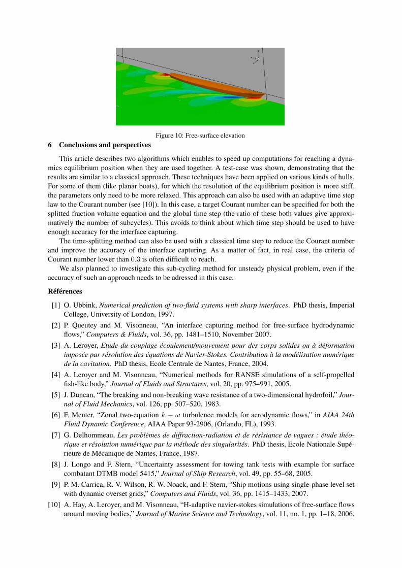
Figure 10: Free-surface elevation6 Conclusions and perspectives

This article describes two algorithms which enables to speed up computations for reaching a dyna-mics equilibrium position when they are used together. A test-case was shown, demonstrating that theresults are similar to a classical approach. These techniques have been applied on various kinds of hulls.For some of them (like planar boats), for which the resolution of the equilibrium position is more stiff,the parameters only need to be more relaxed. This approach can also be used with an adaptive time steplaw to the Courant number (see [10]). In this case, a target Courant number can be specified for both thesplitted fraction volume equation and the global time step (the ratio of these both values give approxi-matively the number of subcycles). This avoids to think about which time step should be used to haveenough accuracy for the interface capturing.

The time-splitting method can also be used with a classical time step to reduce the Courant numberand improve the accuracy of the interface capturing. As a matter of fact, in real case, the criteria ofCourant number lower than 0.3 is often difficult to reach.

We also planned to investigate this sub-cycling method for unsteady physical problem, even if theaccuracy of such an approach needs to be adressed in this case.

Références

[1] O. Ubbink, Numerical prediction of two-fluid systems with sharp interfaces. PhD thesis, ImperialCollege, University of London, 1997.

[2] P. Queutey and M. Visonneau, “An interface capturing method for free-surface hydrodynamicflows,” Computers & Fluids, vol. 36, pp. 1481–1510, November 2007.

[3] A. Leroyer, Etude du couplage écoulement/mouvement pour des corps solides ou à déformationimposée par résolution des équations de Navier-Stokes. Contribution à la modélisation numériquede la cavitation. PhD thesis, Ecole Centrale de Nantes, France, 2004.

[4] A. Leroyer and M. Visonneau, “Numerical methods for RANSE simulations of a self-propelledfish-like body,” Journal of Fluids and Structures, vol. 20, pp. 975–991, 2005.

[5] J. Duncan, “The breaking and non-breaking wave resistance of a two-dimensional hydrofoil,” Jour-nal of Fluid Mechanics, vol. 126, pp. 507–520, 1983.

[6] F. Menter, “Zonal two-equation k − ω turbulence models for aerodynamic flows,” in AIAA 24thFluid Dynamic Conference, AIAA Paper 93-2906, (Orlando, FL), 1993.

[7] G. Delhommeau, Les problèmes de diffraction-radiation et de résistance de vagues : étude théo-rique et résolution numérique par la méthode des singularités. PhD thesis, Ecole Nationale Supé-rieure de Mécanique de Nantes, France, 1987.

[8] J. Longo and F. Stern, “Uncertainty assessment for towing tank tests with example for surfacecombatant DTMB model 5415,” Journal of Ship Research, vol. 49, pp. 55–68, 2005.

[9] P. M. Carrica, R. V. Wilson, R. W. Noack, and F. Stern, “Ship motions using single-phase level setwith dynamic overset grids,” Computers and Fluids, vol. 36, pp. 1415–1433, 2007.

[10] A. Hay, A. Leroyer, and M. Visonneau, “H-adaptive navier-stokes simulations of free-surface flowsaround moving bodies,” Journal of Marine Science and Technology, vol. 11, no. 1, pp. 1–18, 2006.

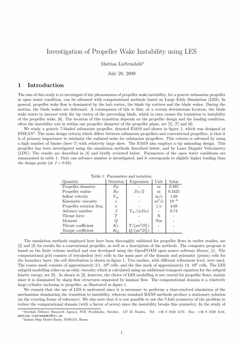
Investigation of Propeller Wake Instability using LES

Mattias Liefvendahl∗

July 20, 2009

1 Introduction

The aim of this study is to investigate if the phenomenon of propeller wake instability, for a generic submarine propellerin open water condition, can be adressed with computational methods based on Large Eddy Simulation (LES). Ingeneral, propeller wake flow is dominated by the hub vortex, the blade tip vortices and the blade wakes. During themotion, the blade wakes are deformed. A consequence of this is that, at a certain downstream location, the bladewake starts to interact with the tip vortex of the preceeding blade, which in turn causes the transition to instabilityof the propeller wake, [6]. The location of this transition depends on the propeller design and the loading condition,often the instability sets in within one propeller diameter of the propeller plane, see [5], [7] and [6].

We study a generic 7-bladed submarine propeller, denoted E1619 and shown in figure 1, which was designed atINSEAN1. The main design criteria which differs between submarine propellers and conventional propellers, is that itis of primary importance to minimize the radiated noise for submarine propellers. This criteria is adressed by usinga high number of blades (here 7) with relatively large skew. The E1619 also employs a tip unloading design. Thispropeller has been investigated using the simulation methods described below, and by Laser Doppler Velocimetry(LDV). The results are described in [4] and briefly reviewed below. Parameters of the open water conditions aresummarized in table 1. Only one advance number is investigated, and it corresponds to slightly higher loading thanthe design point (at J = 0.85).

Table 1: Parameters and notation.

Quantity Notation Expression Unit ValuePropeller diameter DP - m 0.485Propeller radius RP DP /2 m 0.2425Inflow velocity V∞ - m/s 1.68Kinematic viscosity ν - m2/s 10−6

Propeller rotation freq. n - 1/s 4.68Advance number J V∞/(nDP ) - 0.74Thrust force T - N -Moment Q - Nm -Thrust coefficient KT T/(ρn2D4

P ) - -Torque coefficient KQ Q/(ρn2D5

P ) - -

The simulation methods employed here have been thoroughly validated for propeller flows in earlier studies, see[2] and [3] for results for a conventional propeller, as well as a description of the methods. The computer program isbased on the finite volume method and was developed using the OpenFOAM open source software library, [1]. Thecomputational grid consists of tetrahedral (tet) cells in the main part of the domain and prismatic (prism) cells forthe boundary layer, the cell distribution is shown in figure 1. Two meshes, with different refinement level, were used.The coarse mesh consists of approximately 2.5 · 106 cells, and the fine mesh of approximately 13 · 106 cells. The LESsubgrid-modelling relies on an eddy viscosity which is calculated using an additional transport equation for the subgridkinetic energy, see [9]. As shown in [2], however, the choice of LES modelling is not crucial for propeller flows, mainlysince it is dominated by sharp flow structures separated by laminar flow. The computational domain is a relativelylarge cylinder enclosing to propeller, as illustrated in figure 1.

We remark that the use of LES is motivated since it is necessary to performe a time-resolved simulation of themechanisms dominating the transition to instability, whereas standard RANS methods produce a stationary solution(in the rotating frame of reference). We also note that it is not possible to use the 7-fold symmetry of the problem toreduce the computational domain (with a factor of seven) since the instability breaks this symmetry. In the study of

∗Swedish Defence Research Agency, FOI, Stockholm, Sweden. 147 25 Tumba. Tel: +46 8 5550 4170. Fax: +46 8 5550 4144.

mattias.liefvendahl@foi.se

1Italian Ship Model Basin, INSEAN, Rome.

1

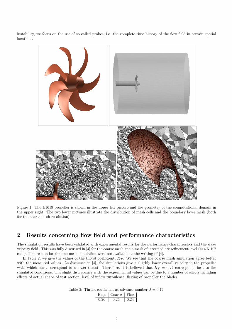
instability, we focus on the use of so called probes, i.e. the complete time history of the flow field in certain spatiallocations.

Figure 1: The E1619 propeller is shown in the upper left picture and the geometry of the computational domain inthe upper right. The two lower pictures illustrate the distribution of mesh cells and the boundary layer mesh (bothfor the coarse mesh resolution).

2 Results concerning flow field and performance characteristics

The simulation results have been validated with experimental results for the performance characterstics and the wakevelocity field. This was fully discussed in [4] for the coarse mesh and a mesh of intermediate refinement level (≈ 4.5·106

cells). The results for the fine mesh simulation were not available at the writing of [4].In table 2, we give the values of the thrust coefficient, KT . We see that the coarse mesh simulation agree better

with the measured values. As discussed in [4], the simulations give a sligthly lower overall velocity in the propellerwake which must correspond to a lower thrust. Therefore, it is believed that KT = 0.24 corresponds best to thesimulated conditions. The slight discrepancy with the experimental values can be due to a number of effects includingeffects of actual shape of test section, level of inflow turbulence, flexing of propeller the blades.

Table 2: Thrust coefficient at advance number J = 0.74.

Exp. Coarse Fine0.26 0.26 0.24

2

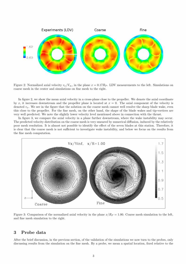
Figure 2: Normalized axial velocity vx/V∞, in the plane x = 0.17RP . LDV measurements to the left. Simulations oncoarse mesh in the center and simulations on fine mesh to the right.

In figure 2, we show the mean axial velocity in a cross-plane close to the propeller. We denote the axial coordinateby x, it increases downstream and the propeller plane is located at x = 0. The axial component of the velocity isdenoted vx. We see in the figure that the solution on the coarse mesh cannot well resolve the sharp blade wake, eventhis close to the propeller. For the fine mesh, on the other hand, the shape of the blade wakes and tip-vortices arevery well predicted. We note the slightly lower velocity level mentioned above in connection with the thrust.

In figure 3, we compare the axial velocity in a plane further downstream, where the wake instability may occur.The predicted velocity distribution on the coarse mesh is very smeared by numerical diffusion, induced by the relativelypoor mesh resolution. It is almost not possible to identify the effect of the seven blades at this station. Therefore, itis clear that the coarse mesh is not sufficient to investigate wake instability, and below we focus on the results fromthe fine mesh computation.

Figure 3: Comparison of the normalized axial velocity in the plane x/RP = 1.00. Coarse mesh simulation to the left,and fine mesh simulation to the right.

3 Probe data

After the brief discussion, in the previous section, of the validation of the simulations we now turn to the probes, onlydiscussing results from the simulation on the fine mesh. By a probe, we mean a spatial location, fixed relative to the

3

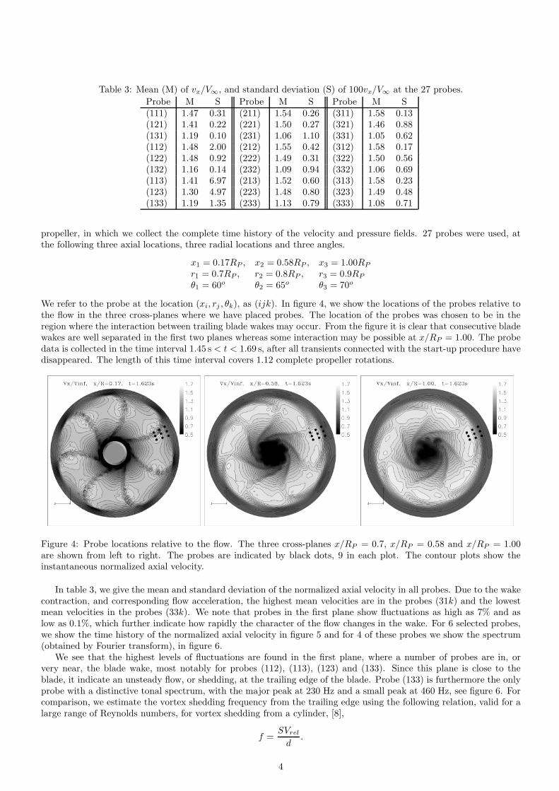
Table 3: Mean (M) of vx/V∞, and standard deviation (S) of 100vx/V∞ at the 27 probes.

Probe M S Probe M S Probe M S(111) 1.47 0.31 (211) 1.54 0.26 (311) 1.58 0.13(121) 1.41 0.22 (221) 1.50 0.27 (321) 1.46 0.88(131) 1.19 0.10 (231) 1.06 1.10 (331) 1.05 0.62(112) 1.48 2.00 (212) 1.55 0.42 (312) 1.58 0.17(122) 1.48 0.92 (222) 1.49 0.31 (322) 1.50 0.56(132) 1.16 0.14 (232) 1.09 0.94 (332) 1.06 0.69(113) 1.41 6.97 (213) 1.52 0.60 (313) 1.58 0.23(123) 1.30 4.97 (223) 1.48 0.80 (323) 1.49 0.48(133) 1.19 1.35 (233) 1.13 0.79 (333) 1.08 0.71

propeller, in which we collect the complete time history of the velocity and pressure fields. 27 probes were used, atthe following three axial locations, three radial locations and three angles.

x1 = 0.17RP , x2 = 0.58RP , x3 = 1.00RP

r1 = 0.7RP , r2 = 0.8RP , r3 = 0.9RP

θ1 = 60o θ2 = 65o θ3 = 70o

We refer to the probe at the location (xi, rj , θk), as (ijk). In figure 4, we show the locations of the probes relative tothe flow in the three cross-planes where we have placed probes. The location of the probes was chosen to be in theregion where the interaction between trailing blade wakes may occur. From the figure it is clear that consecutive bladewakes are well separated in the first two planes whereas some interaction may be possible at x/RP = 1.00. The probedata is collected in the time interval 1.45 s < t < 1.69 s, after all transients connected with the start-up procedure havedisappeared. The length of this time interval covers 1.12 complete propeller rotations.

Figure 4: Probe locations relative to the flow. The three cross-planes x/RP = 0.7, x/RP = 0.58 and x/RP = 1.00are shown from left to right. The probes are indicated by black dots, 9 in each plot. The contour plots show theinstantaneous normalized axial velocity.

In table 3, we give the mean and standard deviation of the normalized axial velocity in all probes. Due to the wakecontraction, and corresponding flow acceleration, the highest mean velocities are in the probes (31k) and the lowestmean velocities in the probes (33k). We note that probes in the first plane show fluctuations as high as 7% and aslow as 0.1%, which further indicate how rapidly the character of the flow changes in the wake. For 6 selected probes,we show the time history of the normalized axial velocity in figure 5 and for 4 of these probes we show the spectrum(obtained by Fourier transform), in figure 6.

We see that the highest levels of fluctuations are found in the first plane, where a number of probes are in, orvery near, the blade wake, most notably for probes (112), (113), (123) and (133). Since this plane is close to theblade, it indicate an unsteady flow, or shedding, at the trailing edge of the blade. Probe (133) is furthermore the onlyprobe with a distinctive tonal spectrum, with the major peak at 230 Hz and a small peak at 460 Hz, see figure 6. Forcomparison, we estimate the vortex shedding frequency from the trailing edge using the following relation, valid for alarge range of Reynolds numbers, for vortex shedding from a cylinder, [8],

f =SVrel

d.

4

1.4

1.402

1.404

1.406

1.408

1.41

1.45 1.5 1.55 1.6 1.65

Probe (121)

1.16

1.18

1.2

1.22

1.24

1.45 1.5 1.55 1.6 1.65

Probe (133)

1.53

1.535

1.54

1.545

1.55

1.45 1.5 1.55 1.6 1.65

Probe (211)

1.46

1.47

1.48

1.49

1.5

1.51

1.45 1.5 1.55 1.6 1.65

Probe (223)

1.57

1.575

1.58

1.585

1.59

1.45 1.5 1.55 1.6 1.65

Probe (313)

1.43

1.44

1.45

1.46

1.47

1.48

1.45 1.5 1.55 1.6 1.65

Probe (321)

Figure 5: Time history of normalized axial velocity vx/V∞, at six different probes. Observe that the scale on thevertical axis is adapted to the range of variation of the different curves.

Here S ≈ 0.21 is the Strouhal number, Vrel ≈ 3.5 m/s is flow velocity relative to the blade and d ≈ 0.005 m is thethickness of the blade. This estimate gives a shedding frequency f = 147 Hz, which is not unreasonable, consideringthe degree of approximation involved. The other probes in the blade wake does not however show any clear peaks.All signals contain virtually no contributions at frequencies above 500 Hz, which is well below the frequency resolvedby the simulation, which employs a time step of ∆t = 2 · 10−5 s.

4 Concluding remarks

The wake field of a generic submarine propeller in open water conditions have been investigated using LES on twomesh refinement levels. A particular focus was to investigate the wake instability. Due to numerical diffusion of thesharp flow structures, the coarse mesh is not sufficient to adress instability. The resolution on the fine mesh maysuffice to investigate this phenomena. The processing of the probe data illustrate that the detailed time-history of theflow can be captured, at least downstream to x/RP ≈ 0.5. Further probe locations will be investigated. Simulation ofa longer time interval allows for the resolution of lower frequencies, which may be crucial for the onset of instability.

5 Acknowledgements

The author thanks Mario Felli and Fabio Di Felice at INSEAN for valuable discussions and explanations concerningthe experimental data and the mechanics of wake instability. I would also like to thank Michel Chapuis, Carl Troeng

5

0

5

10

15

20

0 100 200 300 400 500 600

Probe (121)

0

10

20

30

40

50

60

70

80

0 100 200 300 400 500 600

Probe (133)

0

5

10

15

20

25

30

35

40

0 100 200 300 400 500 600

Probe (223)

0

5

10

15

20

25

30

35

40

0 100 200 300 400 500 600

Probe (321)

Figure 6: Spectrum for probe data, corresponding to four of the probe “signals” in figure 5. The frequency, in Hz, isshown on the horizontal axis.

and Urban Svennberg at FOI for assistance with computational aspects of the study, including mesh generation andpost-processing. The swedish armed forces are acknowledged for their financial support.

References

[1] OpenFOAM 1.3 User Guide, 2006. www.opencfd.co.uk.

[2] R. E. Bensow and M. Liefvendahl. Implicit and explicit subgrid modeling in les applied to a marine propeller.(AIAA-2008-4144), 2008.

[3] R. E. Bensow, M. Liefvendahl, and N. Wikstrom. Propeller Near Wake Analysis using LES with a Rotating Mesh.In 26th Symposium on Naval Hydrodynamics, Rome, Italy, September 2006.

[4] F. Di Felice, M. Felli, M. Liefvendahl, and U. Svennberg. Numerical and experimental analysis of the wakebehaviour of a generic submarine propeller. In 1st International Symposium on Marine Propulsors, June 2009.Trondheim, Norway.

[5] F. Di Felice, D. Di Florio, M. Felli, and G. P. Romano. Experimental investigation of the propeller wake at differentloading conditions by particle image velocimetry. J. Ship Research, 48(2):168–190, 2004.

[6] M. Felli, F. Di Felice, G. Guj, and R. Camussi. Analysis of the propeller wake by pressure and velocity phasemeasurements. Experiments in Fluids, (1), 2006.

[7] M. Felli, G. Guj, and R. Camussi. Effect of the number of blades on propeller wake evolution. In Exponaval 2008,

Vina De Mar, Chile, 2008.

[8] H. Schlichting. Boundary-layer theory. McGraw-Hill, 7 edition, 1979.

[9] U. Schumann. Subgrid scale model for finite difference simulation of turbulent flows in plane channels and annuli.J.Comp.Phys., 18(4):376–404, 1975.

6

1

Numerical Simulations of Unsteady Cavitation Using OpenFOAM

NaiXian Lu, Rickard Bensow

Department of Shipping and Marine Technology,

Chalmers University of Technology, SE 412 96 Gothenburg, Sweden

Email: naixian.lu@chalmers.se

1. INTRODUCTION Numerical simulation of unsteady cavitation is an area that receives increasing attention, both from an

industrial design point of view as well as for an increased understanding of cavitation physics. The industrial need, concerning the design of e.g. marine propellers or hydro turbines, is easily understandable since the cavitation behavior often is the limiting design phenomena; improved prediction tools can increase efficiency and reduce nuisance like erosion, noise and vibration.

This paper deals with the simulation of an unsteady cavitating flow around a 2D NACA15 hydrofoil based on Large Eddy Simulation techniques, combined with a volume of fluid implementation to capture the interface between liquid and vapour and a relatively simple and ad hoc model for the mass transfer between the phases. The unsteady inflow condition is imposed by two oscillators operating at a certain frequency upstream the hydrofoil.

The case is chosen with several interesting aspects in mind. Previous simulations performed on 2D and 3D hydrofoils with steady inflow condition showed a decreasing tendency in terms of the cavity size after the effect of initial cavities is eliminated. Therefore getting a stabilized size of the cavity as the simulation time goes further is of main interest. Moreover, the locking effect between the shedding frequency of the oscillators and cavity is to be studied. Vortex cavity interaction and the transport downstream should also be investigated. This simple 2D case also serves in the purpose to study the moving mesh technique with automatic adaptation in OpenFOAM. The intention is to extend the technique to the 3D Delft foil in unsteady inflow. 2. SIMULATING CAVITATING FLOWS

The flow is treated as incompressible and Newtonian, governed by equations consisting of the balance equations of mass and momentum. An implicit LES approach is employed to model the flow, together with a Spalding wall model to take care of the near wall modeling such that

y+ = u+ +1eκB

eκu+− 1+κu+ +

κ 2u+2

2+κ 3u+3

6⎛

⎝ ⎜ ⎞

⎠ ⎟ ⎧ ⎨ ⎪

⎩ ⎪

⎫ ⎬ ⎪

⎭ ⎪ (1)

where

u+ = u /uτ ,

y+ = uτ y /ν ,

uτ = τ w /ρ and constants

κ = 0.41 and B = 5.0 [3] (2) The interface between liquid and vapour is captured by a Volume of Fluid (VOF) method, and Kunz’ mass transfer model is engaged to model the mass transfer process between the two phases. Refer to Bensow (2008) for further details. 3. NUMERICAL METHOD

The simulations are performed using a finite volume method for arbitrary cell-shapes together with a segregated solver, implemented using the OpenFOAM libraries. A multi-step scheme is used for the time discretization. To complete the FV-discretization the fluxes need to be reconstructed from grid variables at adjacent cells. This requires interpolation of the convective fluxes and difference approximations for the inner derivatives of the diffusive fluxes, preferably of second order accuracy. Since the present methodology is based on implicit modelling of the subgrid stress tensor B, a slightly diffuse scheme is needed to make the leading order truncation error act as the modelling of the subgrid stress tensor. This can be performed using different kind of limiters and schemes, and in the present simulations simple forms of implicit subgrid stress modelling are used based on linear blending of up-winding and central differencing interpolation.

A Poisson equation is used to handle the pressure-velocity coupling in the incompressible flow equations and this equation is solved via the PISO (Pressure Implicit with Splitting of Operators) procedure based on a Rhie&Chow-like interpolation for cell-centred data, (Issa 1986). The cavitation sources are incorporated into the equation as source terms in the continuity equation, i.e. in the Poisson equation, and in the volume fraction equation. In the volume fraction equation the source term is included explicitly while in the Poisson equation the source term is split into one explicit and one implicit term for increased stability. The splitting is performed as

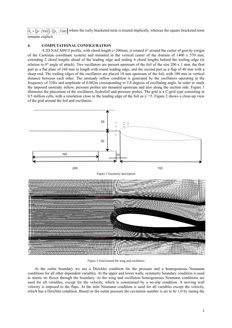
2

where the curly bracketed term is treated implicitly, whereas the square bracketed term remains explicit.

4. COMPUTATIONAL CONFIGURATION

A 2D NACA0015 profile, with chord length c=200mm, is rotated 6° around the center of gravity (origin of the Cartesian coordinate system) and mounted in the vertical center of the domain of 1400 x 570 mm, extending 2 chord lengths ahead of the leading edge and ending 4 chord lengths behind the trailing edge (in relation to 0° angle of attack). Two oscillators are present upstream of the foil of the size 200 x 1 mm, the first part as a flat plate of 160 mm in length with round leading edge, and the second part as a flap of 40 mm with a sharp end. The trailing edges of the oscillators are placed 10 mm upstream of the foil, with 100 mm in vertical distance between each other. The unsteady inflow condition is generated by the oscillators operating at the frequency of 32Hz and amplitude of 0.002m corresponding to 5.8 degrees of oscillating angle. In order to study the imposed unsteady inflow, pressure probes are mounted upstream and also along the suction side. Figure 1 illustrates the placement of the oscillators, hydrofoil and pressure probes. The grid is a C-grid type consisting in 0.5 million cells, with a resolution close to the leading edge of the foil as y+=5. Figure 2 shows a close-up view of the grid around the foil and oscillators.

Figure 1 Geometry description

Figure 2 Grid around the wing and oscillators

At the outlet boundary we use a Dirichlet condition for the pressure and a homogeneous Neumann conditions for all other dependent variables. At the upper and lower walls, symmetry boundary condition is used to mimic no fluxes through the boundary. At the wing and oscillators homogeneous Neumann conditions are used for all variables, except for the velocity, which is constrained by a no-slip condition. A moving wall velocity is imposed to the flaps. At the inlet Neumann condition is used for all variables except the velocity, which has a Dirichlet condition. Based on the outlet pressure the cavitaiton number is set to be 1.0 by tuning the

3

vaporization pressure. Physical values are used for the densities of the two phases, and they are set to ρl=998 for the liquid and for the vapour ρv=0.023. For other specific data, see table 1.

The simulation is started without the cavitation sources activated and is continued in non-cavitating flow conditions until the first order statistical moments have converged. Thereafter, the cavitation sources are gradually increased from zero to full value over a number of time steps and the cavitation starts. Inlet velocity 6 m/s Outlet pressure 29700 Pa

Angular velocity 201.06 r/s Flap Amplitude 0.002 m Vaporization pressure 11736 Pa

Table 1. Computational configurations

5. DISCUSSION OF RESULT

Coordinates of pressure probes:

1 (-0.071 0.026) 2 (-0.071 0.016)

3 (-0.071 0.006) 4 (-0.071 -0.004)

5 (-0.051 0.026) 6 (-0.051 0.021)

6 (-0.051 0.016) 8 (-0.041 0.026)

9 (-0.041 0.021)

Figure 3 Wetted flow, pressure probes

The top four curves in Figure 3 represent the four probes located upstream of the foil, while the probes above the foil suction side are represented by the bottom five curves, averaged variation frequency for all the probes over three oscillating cycles are listed in table 2. The minimum values of the upstream pressure probes occur when the oscillators have just reached their uppermost positions and move back to the original positions, while the maximum values occur when the oscillators move from their bottommost positions to the origins. From the figure a delay between the time when upstream probes and suction side probes have reached their peak values can be observed, and also the pressure fluctuation is amplified by the presence of the foil. In one oscillating cycle, the minimum value of the pressure coefficient varies from -1.06 to -1.31.

Probe 1 Probe 2 Probe 3 Probe 4 Probe 5 Probe 6 Probe 7 Probe 8 Probe 9

32.19 31.97 32.03 31.32 31.93 31.87 31.72 32.08 31.94 Table 2. Shedding frequencies of probes pressure

4

Figure 4 Wetted flow, pressure coefficients

Preliminary result of cavitating flow has several defects. Figure 5 illustrates a sequence of instantaneous vapour volume fraction, with comparison between the results obtained under unsteady (upper figure in each snapshot) and steady inflow condition (bottom figure [5]). The three snapshots are not taken in the same cavity cycle, but in the aim to show the difference in the captured mechanism of two flow conditions. Cavitation numbers are both 1. In Figure 5.a, initial cavity has reached its maximum length and cavity shape of the unsteady inflow case is shorter in length and much thinner in thickness. In Figure 5.b, the cut-offs of the cavity are visible in both cases, but the re-entrant jet is too weak in the unsteady case thus doesn’t necessarily result in cut-off in every cycle. In Figure 5.c, the periodic shed vortices with isolated cavity bubbles caused by the shear layer between the free stream and back flow are captured in the steady case together with a upstream collapse towards the leading edge. However in the unsteady case this important mechanism is not captured.

(a) (b)

(c) Figure 5 Development of cavities, vapour volume fractio

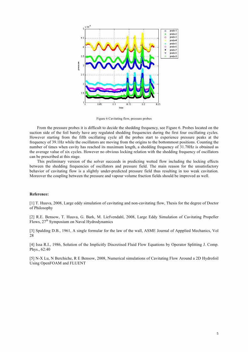
5

Figure 6 Cavitating flow, pressure probes

From the pressure probes it is difficult to decide the shedding frequency, see Figure 6. Probes located on the suction side of the foil barely have any regulated shedding frequencies during the first four oscillating cycles. However starting from the fifth oscillating cycle all the probes start to experience pressure peaks at the frequency of 39.1Hz while the oscillators are moving from the origins to the bottommost positions. Counting the number of times when cavity has reached its maximum length, a shedding frequency of 31.78Hz is obtained as the average value of six cycles. However no obvious locking relation with the shedding frequency of oscillators can be prescribed at this stage.

This preliminary version of the solver succeeds in predicting wetted flow including the locking effects between the shedding frequencies of oscillators and pressure field. The main reason for the unsatisfactory behavior of cavitating flow is a slightly under-predicted pressure field thus resulting in too weak cavitation. Moreover the coupling between the pressure and vapour volume fraction fields should be improved as well. Reference:

[1] T. Huuva, 2008, Large eddy simulation of cavitating and non-cavitating flow, Thesis for the degree of Doctor of Philosophy

[2] R.E. Bensow, T. Huuva, G. Bark, M. Liefvendahl, 2008, Large Eddy Simulation of Cavitating Propeller Flows, 27th Symposium on Naval Hydrodynamics

[3] Spalding D.B., 1961, A single formular for the law of the wall, ASME Journal of Appplied Mechanics, Vol 28

[4] Issa R.I., 1986, Solution of the Implicitly Discretised Fluid Flow Equations by Operator Splitting J. Comp. Phys., 62:40

[5] N-X Lu, N Berchiche, R E Bensow, 2008, Numerical simulations of Cavitating Flow Around a 2D Hydrofoil Using OpenFOAM and FLUENT

Maneuvering Simulations of Underwater Vehicles

Lars Ole Lubke (luebke@sva-potsdam.de)

Potsdam Model Basin

Introduction

In the offshore industry as well as for research worka variety of tasks have to be carried out subsea,covering inspection services for pipelines or cables,research missions investigating the underwater lifeor exploring natural resources. These tasks re-quire suitable carriers/vehicles equipped with sen-sors, cameras, probes or manipulators. For thedifferent requirements, different design have beenestablished. DSVs (Deep Sea Vehicle), mannedsubmarines, ROVs (Remotely Operated Vehicle),unmanned vehicles connected via cables with theirmother ship, and AUVs (Autonomous UnderwaterVehicle), also unmanned vehicles, are operated.

To guarantee the safety of vehicle and crew as wellas to assure the operability in the specified condi-tions the maneuvreability of the subsea vehicle hasto be known in advance, making maneuvering testsnecessary. Besides the possibility to carry out di-rect maneuvering tests, different approaches existto determine the maneuverability. The approachcarried out at the Potsdam Model Basin (SVA)is based on the formulation of a mathematical se-ries to describe the external forces and momentsin the equations of motion acting upon the vehicle.The coefficients of the series can be determined ex-perimentally or numerically. Once the coefficientsare known arbitrary maneuvers can be simulated.The coefficients can be determined by the mea-surement of the forces and moments in SUBPMM(SUBmarine Planar Motion Mechanism) tests or bythe measurement of the velocities and accelerationsof a free maneuvering vehicle and a preceeding sys-tem identification. Also numerical methods can beapplied to calculate the hydrodynamic coefficients,having the advantage that testing is not influencedby the limitations of the testing facilities and thatthe calculations can be carried out for the full-scaleRe number.

The focus of this paper is laid upon the nu-merical simulation of planar motion and statictests to determine the hydrodynamic coefficients.The intention is to investigate the applicabilityof RANSE-methods (Reynolds-averaged Navier-

Stokes equations) to perform maneuvering simula-tions. The numerical calculations were validatedwith the available experimental results.

For the investigations one DSV and one AUV wereselected.

Geometry and numerical mesh

Two vessels were investigated.

• DSV, scale λ=1 and λ=10

• AUV, scale λ=1

The DSV (submarine) has a x-rudder, a forwardfin and is of length LPP ≈ 60m. The AUV is atwin-screw vessel with a conventional rudder (pitchand yaw rudder), nozzle propellers and is of lengthLPP ≈ 3.50m.

The numerical meshes for the calculations were gen-erated with the commercial software ANSYS ICEMCFD. In general block-structured meshes consistingout of hexahedral elements were employed, exceptfor the DSV with inclined rudder, where a hybridapproach was chosen. In this case the rudder bladesand the near surrounding were meshed with tetra-hedral elements and a prismatic sublayer. This ap-proach has proven to be advantageous with respectto the meshing in the rudder gaps[4]. Symmetryaround the midships plane was employed when everpossible.

In order to impose the propeller forces of a bodyforce model in the solution domain, a subdomainat the propeller position, with the radial extensionsequal to the propeller diameter, was defined.

For the dynamic simulations of predefined motions,mesh motion techniques were used. For these appli-cations an additional subdomain was defined whichfully encloses the vehicles with all appendages. Themesh deformations were only allowed outside of thissubdomain, guaranteeing identical meshes closelyaround the vehicles during the simulations.

In case of the DSV special attention was laid uponobtaining values for the dimensionless wall distance

Page 1

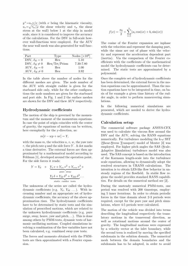
y+=uτy/ν (with ν being the kinematic viscosity,uτ=

√τw/ρ the shear velocity and τw the shear

stress at the wall) below 1 at the ship in modelscale, since it is considered to improve the accuracyof the calculations. For the DSV in full-scale how-ever wall-functions were employed. For the AUVthe near wall mesh was also generated for wall func-tions.

Part Type Nodes [×106]DSV, δR = 0 Hex 5.10DSV, δR 6= 0 Hex/Tet/Prism 7.30-7.80AUV, δR = 0 Hex 1.00AUV, δR 6= 0 Hex 3.92

In the table above the number of nodes for thedifferent meshes are given. The node number ofthe AUV with straight rudder is given for thestarboard side only, while for the other configura-tions the node numbers are given for the starboardand port side. In Fig. 1 and 2 the surface meshesare shown for the DSV and thew AUV respectively.

Hydrodynamic coefficients

The motion of the ship is governed by the momen-tum and the moment of the momentum equations.In case the point of origin coincides with the centerof gravity, the equations of motion can be written,here exemplarily for the y-direction, as:

m[v − wp + ur] = Y,

with the mass m, the velocities u, v, w, the yaw rater, the pitch rate q and the side force Y . A dot marksa time derivative. The external forces are then ap-proximated by a mathematical model according toFeldman [1], developed around the operation point.For the side forces it reads:

Y = Y0 + Yv v + Yvv v2 + Yvvv v3

︸ ︷︷ ︸pure sway

+

Yδ δ + Yδδ δ2 + Yδδδ δ3

︸ ︷︷ ︸static rudder tests

. . .

The unknowns of the series are called the hydro-dynamic coefficients (e.g. Yδ, Yδδ . . . ). With in-creasing number and an appropriate set of hydro-dynamic coefficients, the accuracy of the above ap-proximation rises. The hydrodynamic coefficientshave to be determined by static tests and the sim-ulation of prescribed motions, which are related tothe unknown hydrodynamic coefficients (e.g. puresurge, sway, heave, yaw and pitch. . . ). This is doneamong others by PMM-tests, dynamic tests of har-monic oscillating motions. Coupled simulations in-volving a combination of the free variables have notbeen calculated, e.g. combined sway-yaw tests.

The forces and moments obtained with the PMM-tests are then approximated with a Fourier expan-sion.

f(x) =a0

2+

n∑

i=1

(ai cos(ix) + bi sin(ix))

The cosine of the Fourier expansion are inphasewith the velocities and represent the damping part,while the sinus are out of phase with the veloc-ity and represent the acceleration dependent part(inertia). Via the comparison of the Fourier co-efficients with the coefficients of the mathematicalmodel the hydrodynamic coefficients can be deter-mined. The static tests are approximated by apolynomial.

Once the complete set of hydrodynamic coefficientshas been determined, the external forces in the mo-tion equations can be approximated. Than the mo-tion equations have to be integrated in time, on ba-sis of for example a given time history of the rud-der angle, in order to perform maneuvering simu-lations.

In the following numerical simulations arepresented, which are needed to derive the hydro-dynamic coefficients.

Calculation setup

The commercial software package ANSYS-CFXwas used to calculate the viscous flow around theDSV and the AUV, solving the RANS equationsnumerically. For turbulence modeling the k-ω SST(Shear-Stress Transport) model of Menter [3] wasemployed. For higher pitch angles the SAS (Scale-Adaptive Simulation) turbulence model was alsoused. The SAS concept is based on the introductionof the Karmann length-scale into the turbulencescale equations, allowing to dynamically adopt theresolved structures in URANS calculations. Theintention is to obtain LES-like flow behavior in un-steady regions of the flowfield. In stable flow re-gions the model provides standard RANS capabili-ties. For details on the numerical method see [2].

During the unsteady numerical PMM-tests, oneperiod was resolved with 200 timesteps, employ-ing 5 inner iterations. In order to obtain periodicforces in the time domain about 2-3 periods wererequired, except for the pure yaw and pitch simu-lations, where 4-5 periods were calculated.

The motion of the vehicle was divided into termsdescribing the longitudinal respectively the trans-latory motions in the transversal direction, aswell as rotational motions around the center ofgravity. The longitudinal motions were expressedby a velocity vector at the inlet boundary, whilethe second term is realized by moving the specifiedsubdomain in the solution domain. The numericalmesh between the domain boundaries and thesubdomain has to be adopted, in order to avoid

Page 2

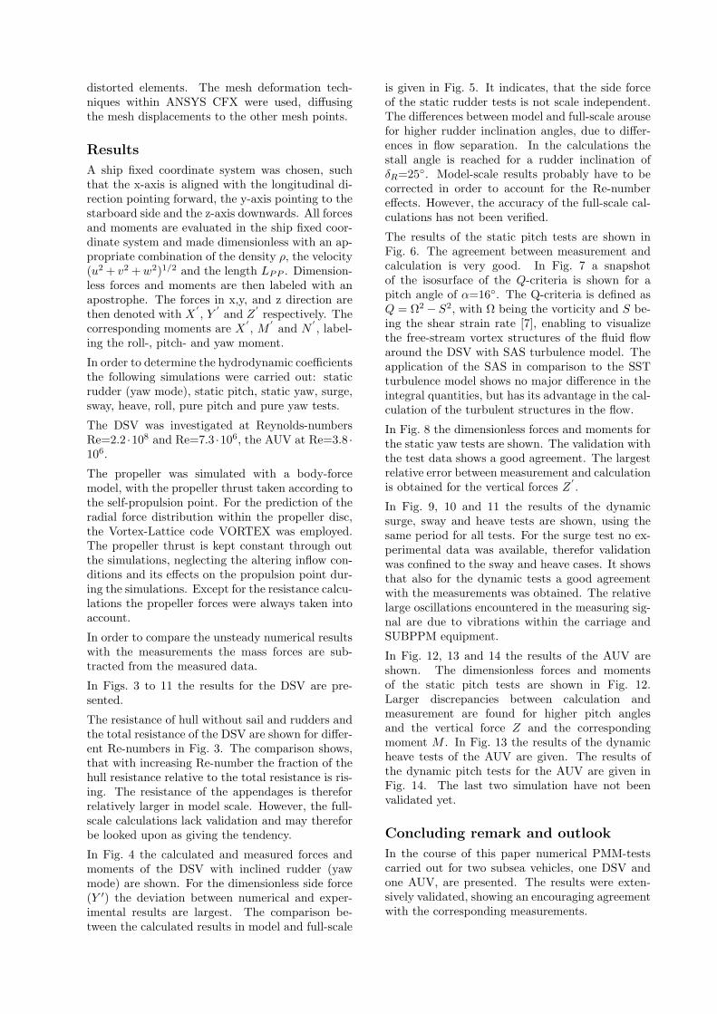
distorted elements. The mesh deformation tech-niques within ANSYS CFX were used, diffusingthe mesh displacements to the other mesh points.

Results

A ship fixed coordinate system was chosen, suchthat the x-axis is aligned with the longitudinal di-rection pointing forward, the y-axis pointing to thestarboard side and the z-axis downwards. All forcesand moments are evaluated in the ship fixed coor-dinate system and made dimensionless with an ap-propriate combination of the density ρ, the velocity(u2 + v2 + w2)1/2 and the length LPP . Dimension-less forces and moments are then labeled with anapostrophe. The forces in x,y, and z direction arethen denoted with X

′, Y

′and Z

′respectively. The

corresponding moments are X′, M

′and N

′, label-

ing the roll-, pitch- and yaw moment.

In order to determine the hydrodynamic coefficientsthe following simulations were carried out: staticrudder (yaw mode), static pitch, static yaw, surge,sway, heave, roll, pure pitch and pure yaw tests.

The DSV was investigated at Reynolds-numbersRe=2.2 ·108 and Re=7.3 ·106, the AUV at Re=3.8 ·106.

The propeller was simulated with a body-forcemodel, with the propeller thrust taken according tothe self-propulsion point. For the prediction of theradial force distribution within the propeller disc,the Vortex-Lattice code VORTEX was employed.The propeller thrust is kept constant through outthe simulations, neglecting the altering inflow con-ditions and its effects on the propulsion point dur-ing the simulations. Except for the resistance calcu-lations the propeller forces were always taken intoaccount.

In order to compare the unsteady numerical resultswith the measurements the mass forces are sub-tracted from the measured data.

In Figs. 3 to 11 the results for the DSV are pre-sented.

The resistance of hull without sail and rudders andthe total resistance of the DSV are shown for differ-ent Re-numbers in Fig. 3. The comparison shows,that with increasing Re-number the fraction of thehull resistance relative to the total resistance is ris-ing. The resistance of the appendages is thereforrelatively larger in model scale. However, the full-scale calculations lack validation and may thereforbe looked upon as giving the tendency.

In Fig. 4 the calculated and measured forces andmoments of the DSV with inclined rudder (yawmode) are shown. For the dimensionless side force(Y ′) the deviation between numerical and exper-imental results are largest. The comparison be-tween the calculated results in model and full-scale

is given in Fig. 5. It indicates, that the side forceof the static rudder tests is not scale independent.The differences between model and full-scale arousefor higher rudder inclination angles, due to differ-ences in flow separation. In the calculations thestall angle is reached for a rudder inclination ofδR=25. Model-scale results probably have to becorrected in order to account for the Re-numbereffects. However, the accuracy of the full-scale cal-culations has not been verified.

The results of the static pitch tests are shown inFig. 6. The agreement between measurement andcalculation is very good. In Fig. 7 a snapshotof the isosurface of the Q-criteria is shown for apitch angle of α=16. The Q-criteria is defined asQ = Ω2 − S2, with Ω being the vorticity and S be-ing the shear strain rate [7], enabling to visualizethe free-stream vortex structures of the fluid flowaround the DSV with SAS turbulence model. Theapplication of the SAS in comparison to the SSTturbulence model shows no major difference in theintegral quantities, but has its advantage in the cal-culation of the turbulent structures in the flow.

In Fig. 8 the dimensionless forces and moments forthe static yaw tests are shown. The validation withthe test data shows a good agreement. The largestrelative error between measurement and calculationis obtained for the vertical forces Z

′.

In Fig. 9, 10 and 11 the results of the dynamicsurge, sway and heave tests are shown, using thesame period for all tests. For the surge test no ex-perimental data was available, therefor validationwas confined to the sway and heave cases. It showsthat also for the dynamic tests a good agreementwith the measurements was obtained. The relativelarge oscillations encountered in the measuring sig-nal are due to vibrations within the carriage andSUBPPM equipment.

In Fig. 12, 13 and 14 the results of the AUV areshown. The dimensionless forces and momentsof the static pitch tests are shown in Fig. 12.Larger discrepancies between calculation andmeasurement are found for higher pitch anglesand the vertical force Z and the correspondingmoment M . In Fig. 13 the results of the dynamicheave tests of the AUV are given. The results ofthe dynamic pitch tests for the AUV are given inFig. 14. The last two simulation have not beenvalidated yet.

Concluding remark and outlook

In the course of this paper numerical PMM-testscarried out for two subsea vehicles, one DSV andone AUV, are presented. The results were exten-sively validated, showing an encouraging agreementwith the corresponding measurements.

Page 3

The evaluation of the numerical results is still inprogress, giving the hydrodynamic coefficients todescribe the external forces in the motion equa-tions. With a complete set of hydrodynamic co-efficients maneuvering simulations can be carriedout. The comparison of the maneuvering simula-tions based on the experimental coefficients withthe ones based on numerical calculations (at leastthe majority) will reveal the potential of the ap-proach and wether it may prove to be an attractivealternative for predicting the ship maneuverability.It is planned to compare the standard maneuveringtest, like for example the zigzag-maneuvers accord-ing to the IMO recommendations.

The required simulation time to obtain a full-setof coefficients is very long, making large compu-tational resources and many solver licenses neces-sary. In order to reduce the computational effort,smaller grid sizes should be considered. Also it mayprove to be more practical to combine both numer-icalyl and experimentally obtained coefficients forthe maneuvering simulations, using RANSE calcu-lations were they may be advantageous.

The presented approach is considered an intermidi-ate step towards the direct simulations of the ma-neuvering tests. In case of a PMM-approach arbi-trary maneuvers can be simulated once the hydro-dynamic coefficients are predicted, with the accu-racy depending on the quality of the approximatedexternal forces in the motion equations. The di-rect simulation of maneuvers is assumed to be moreaccurate, however, depending on the number of re-quired maneuvers, the simulation time may be evenlarger.

The author would further like to express his grati-tude towards the German Federal Ministry for Eco-nomics and Labour for having supported this work.

References

[1] J. FeldmanRevised Standard Submarine Equations ofMotion,David W. Taylor Naval Ship Research and De-velopment Center, DTNSRDC/SPD-0393-09,June 1979

[2] ANSYS-CFX Manual Version 11,April 2007

[3] Menter, F.Two-equation eddy-viscosity turbulence mod-els for engineering applications,AIAA-Journal, 32(8), 1994

[4] L. O. LubkeInvestigation of a Semi-Balanced Rudder,

10th Numerical Towing Tank Symposium, 23-15 April 2007, Hamburg, Germany

[5] R. E. Bensow, C. FurebyLarge Eddy Simulation of Viscous Flowaround a Submarine During Manoeuver,10th Numerical Towing Tank Symposium, 23-15 April 2007, Hamburg, Germany

[6] A. Cura-HochbaumVirtual PMM tests for Manoeuvring Predic-tion,26th Symposium on Naval Hydrodynamics, 17-22 September 2006, Rome, Italy

[7] A. Lifante, T. Frank, K. RieckOn Influence of Turbulence Modelling on Cav-itation Prediction for Flow around P1356 ShipPropeller,27th Conference on Offshore Mechanics andArtic Engineering, OMAE2008, 15-20 June2008, Estoril, Portugal

Figure 1: Numerical mesh of DSV

Figure 2: Numerical mesh of AUV

Page 4

1e+06 1e+07 1e+08 1e+09Re [-]

0

CT

[-]

CT

λ= 1C

Tλ=10

CT

λ=20C

T hull λ= 1

CT hull λ=10

CT hull λ=20

Figure 3: DSV, resistance of hull (without sail) onlyand total resistance

0 5 10 15 20 25 30 δ R [°]

0

X’,

Y’,

N’ [

-]

X’ CFDY’ CFDN’ CFDX’ Exp.

Y’ Exp.

N’ Exp.

Figure 4: DSV, dimensionless forces and moments,static rudder

0 5 10 15 20 25 30 δ R [°]

0

X’,

Y’,

N’ [

-]

X’ λ=10, CFD

Y’ λ=10, CFD

N’ λ=10, CFD

X’ λ= 1, CFD

Y’ λ= 1, CFD

N’ λ= 1, CFD

Figure 5: DSV, dimensionless forces and moments,static rudder tests for model and full scale

-16 -12 -8 -4 0 4 8 12 16 α [°]

0

X’,

Z’,

M’

[-]

X’ CFDZ’ CFDM’ CFDX’ Exp.Z’ Exp.M’ Exp.

Figure 6: DSV, dimensionless forces and moments,static pitch

Figure 7: DSV, vortical structures, static pitch,α=16

-4 0 4 8 12 16 β [°]

0

Y’,

Z’,

N’

[-]

Y’ CFDZ’ CFDN’ CFDY’ Exp.

Z’ Exp.

N’ Exp.

Figure 8: DSV, dimensionless forces and moments,static yaw

Page 5

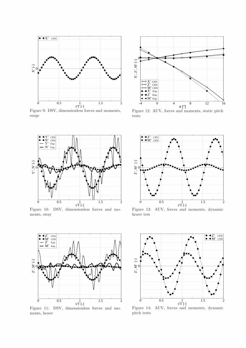
0 0.5 1 1.5 2t/T [-]

0

X’

[-]

X’ CFD

Figure 9: DSV, dimensionless forces and moments,surge

0 0.5 1 1.5 2t/T [-]

0

Y’,

N’

[-]

Y’ CFDN’ CFDY’ Exp.

N’ Exp.

Figure 10: DSV, dimensionless forces and mo-ments, sway

0 0.5 1 1.5 2t/T [-]

0

Z’,

M’

[-]

Z’ CFDM’ CFDZ’ Exp.

M’ Exp.

Figure 11: DSV, dimensionless forces and mo-ments, heave

-4 0 4 8 12 16 α [°]

0

X’,

Z’,

M’

[-]

X’ CFDZ’ CFDM’ CFDX’ Exp.

Z’ Exp.

M’ Exp.

Figure 12: AUV, forces and moments, static pitchtests

0 0.5 1 1.5 2t/T [-]

0

Z’,

M’

[-]

Z’ CFDM’ CFD

Figure 13: AUV, forces and moments, dynamicheave test

0 0.5 1 1.5 2t/T [-]

0

Z’,

M’

[-]

Z’ CFDM’ CFD

Figure 14: AUV, forces and moments, dynamicpitch tests

Page 6

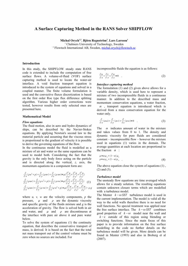
A Surface Capturing Method in the RANS Solver SHIPFLOW

Michal Orych1,2, Björn Regnström2, Lars Larsson1

1 Chalmers University of Technology, Sweden2 Flowtech International AB, Sweden, michal.orych@flowtech.se

Introduction

In this study, the SHIPFLOW steady state RANS code is extended to include the computation of free surface flows. A volume-of-fluid (VOF) surface capturing method is used to locate the water-air interface. A void fraction transport equation is introduced to the system of equations and solved in a coupled manner. The finite volume formulation is used and the convective fluxes discretization is based on the first order Roe type flux difference splitting algorithm. Various higher order corrections were tested, however results from only selected ones are presented here.

Mathematical Model

Flow equationsThe fluid motion, also in aero and hydro dynamics of ships, can be described by the Navier-Stokes equations. By applying Newton's second law to the material particle and assuming that the viscous stress is proportional to the gradient of velocity it is possible to derive the governing equations of the flow. In the continuous model the fluid is modelled as a mixture of air and water so the same equations can be used to model both. Considering the fact that the gravity is the only body force acting on the particle and is directed along the vertical, z, axis, the momentum equations in a component form are:

∂∂ x u2p ∂

∂ y uv ∂∂ z uw= ∂

2 u∂ x 2

∂2 u∂ y 2

∂2 u∂ z2

∂∂ x uv ∂

∂ y v2 p ∂∂ z vw = ∂

2 v∂ x2

∂2 v∂ y2

∂2v∂ z2 (1)

∂∂ x uw ∂

∂ y vw ∂∂ z w2p= ∂

2w∂ x2

∂2 w∂ y2

∂2 w∂ z2 − g

where u, v, w are the velocity components, p the pressure, and are the dynamic viscosity and specific gravity of the fluids mixture and g is the acceleration of gravity. The flow is solved both in air and water, and and are discontinuous at the interface with pure air above it and pure water below. To solve the system of equations (1) the continuity equation, that describes the conservative transport of mass, is derived. It is based on the fact that the total net mass transport out of the control volume must be zero when no sources are included. For

incompressible fluids the equation is as follows:

∂u∂ x

∂v∂ y

∂w∂ z =0 . (2)

Interface capturing methodThe formulation (1) and (2) given above allows for a variable density, which is used here to represent a mixture of two incompressible fluids in a continuous manner. In addition to the described mass and momentum conservation equations, a water fraction, , transport equation is introduced which is

derived from a mass conservation equation for the water only.

∂∂ x u ∂

∂ y v ∂∂ z w=0 . (3)

The indicates amount of water in the mixture and takes values from 0 to 1. The density and dynamic viscosity for pure fluids are considered constant – incompressible flow – however the mixture used in equations (1) varies in the domain. The average quantities at each location are proportional to the fraction :

=w1−a

=w1− a . (4)

The above equation close the system of equations (1) , (2) and (3).

Turbulence modelThe unsteady flow equations are time averaged which allows for a steady solution. The resulting equations contain unknown closure terms which are modelled with a turbulence model. The Menter k−SST turbulence model is used in the current implementation. The model is valid all the way to the solid walls therefore there is no need for wall functions. No special treatment was applied near the free surface interface. The k−SST combines good properties of k− model near the wall and

k− outside of this region using blending or switching functions. Since the main focus of this paper is to provide information on the free surface modelling in the code no further details on the turbulence model will be given. More details can be found in Menter (1993) and also in Broberg et al (2007).

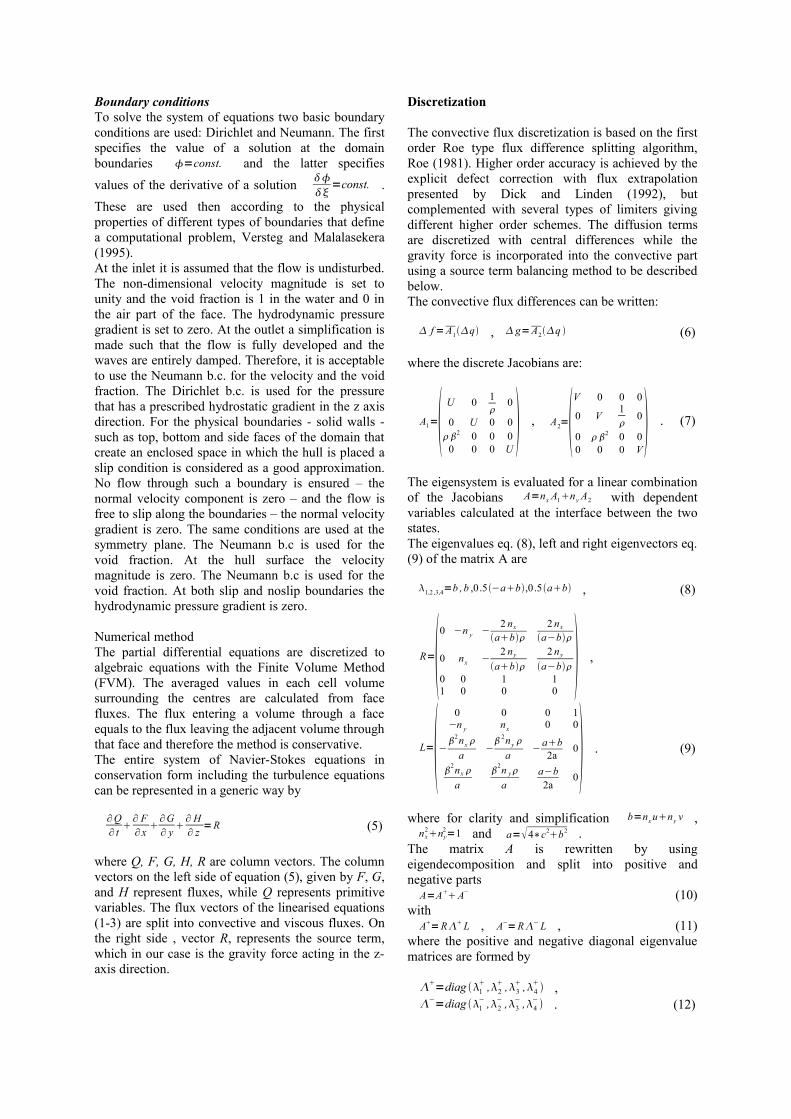
Boundary conditionsTo solve the system of equations two basic boundary conditions are used: Dirichlet and Neumann. The first specifies the value of a solution at the domain boundaries =const. and the latter specifies values of the derivative of a solution

=const. .

These are used then according to the physical properties of different types of boundaries that define a computational problem, Versteg and Malalasekera (1995). At the inlet it is assumed that the flow is undisturbed. The non-dimensional velocity magnitude is set to unity and the void fraction is 1 in the water and 0 in the air part of the face. The hydrodynamic pressure gradient is set to zero. At the outlet a simplification is made such that the flow is fully developed and the waves are entirely damped. Therefore, it is acceptable to use the Neumann b.c. for the velocity and the void fraction. The Dirichlet b.c. is used for the pressure that has a prescribed hydrostatic gradient in the z axis direction. For the physical boundaries - solid walls - such as top, bottom and side faces of the domain that create an enclosed space in which the hull is placed a slip condition is considered as a good approximation. No flow through such a boundary is ensured – the normal velocity component is zero – and the flow is free to slip along the boundaries – the normal velocity gradient is zero. The same conditions are used at the symmetry plane. The Neumann b.c is used for the void fraction. At the hull surface the velocity magnitude is zero. The Neumann b.c is used for the void fraction. At both slip and noslip boundaries the hydrodynamic pressure gradient is zero.

Numerical methodThe partial differential equations are discretized to algebraic equations with the Finite Volume Method (FVM). The averaged values in each cell volume surrounding the centres are calculated from face fluxes. The flux entering a volume through a face equals to the flux leaving the adjacent volume through that face and therefore the method is conservative. The entire system of Navier-Stokes equations in conservation form including the turbulence equations can be represented in a generic way by

∂Q∂ t

∂ F∂x

∂G∂ y

∂ H∂ z =R (5)

where Q, F, G, H, R are column vectors. The column vectors on the left side of equation (5), given by F, G, and H represent fluxes, while Q represents primitive variables. The flux vectors of the linearised equations (1-3) are split into convective and viscous fluxes. On the right side , vector R, represents the source term, which in our case is the gravity force acting in the z-axis direction.

Discretization

The convective flux discretization is based on the first order Roe type flux difference splitting algorithm, Roe (1981). Higher order accuracy is achieved by the explicit defect correction with flux extrapolation presented by Dick and Linden (1992), but complemented with several types of limiters giving different higher order schemes. The diffusion terms are discretized with central differences while the gravity force is incorporated into the convective part using a source term balancing method to be described below.The convective flux differences can be written:

f =A1q , g=A2q (6)

where the discrete Jacobians are:

A1= U 0 1

0

0 U 0 0 2 0 0 0

0 0 0 U , A2=V 0 0 0

0 V 1

0

0 2 0 00 0 0 V

. (7)

The eigensystem is evaluated for a linear combination of the Jacobians A=nx A1ny A2 with dependent variables calculated at the interface between the two states.The eigenvalues eq. (8), left and right eigenvectors eq.(9) of the matrix A are

1,2 ,3,4=b ,b ,0.5−ab,0.5ab , (8)

R=0 −n y −2 nx

ab2 nx

a−b

0 nx −2 ny

ab2 ny

a−b0 0 1 11 0 0 0

,

L=0 0 0 1

−n y nx 0 0

−2nx

a− 2ny

a− ab

2a0

2nx a

2n ya

a−b2a

0 . (9)

where for clarity and simplification b=nx uny v ,nx

2ny2=1 and a=4∗c2b2 .

The matrix A is rewritten by using eigendecomposition and split into positive and negative parts

A=AA− (10)with

A=R L , A−=R− L , (11)where the positive and negative diagonal eigenvalue matrices are formed by

=diag 1 ,2

,3 ,4

,−=diag 1

− ,2− ,3

− ,4− . (12)

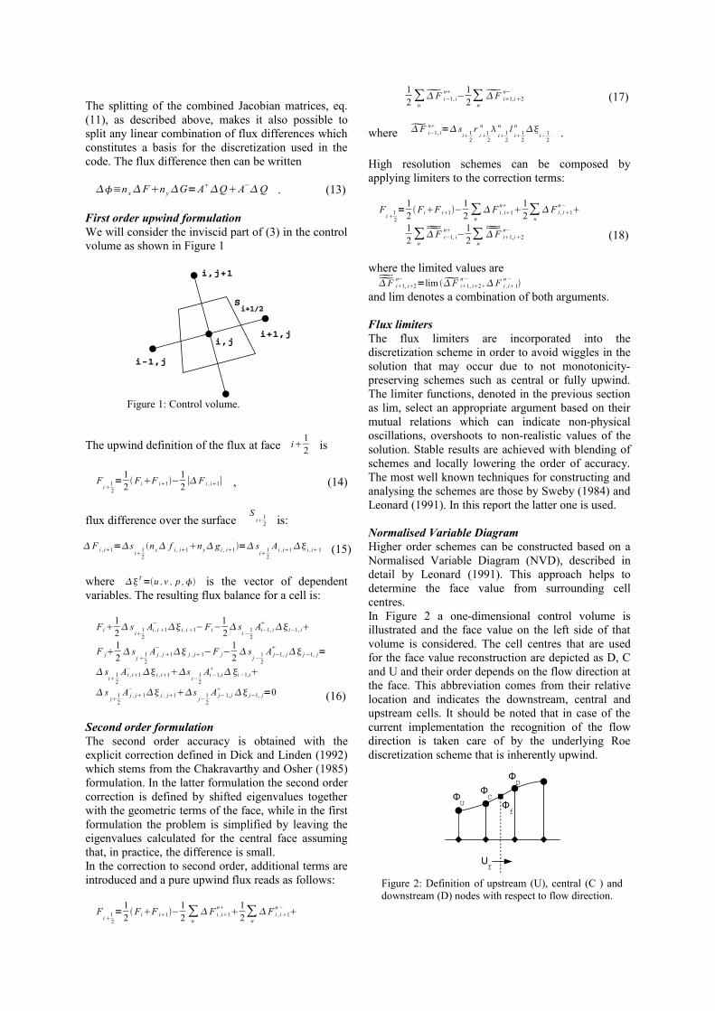
The splitting of the combined Jacobian matrices, eq. (11), as described above, makes it also possible to split any linear combination of flux differences which constitutes a basis for the discretization used in the code. The flux difference then can be written

≡n xFn yG=AQA−Q . (13)

First order upwind formulationWe will consider the inviscid part of (3) in the control volume as shown in Figure 1

The upwind definition of the flux at face i 12 is

Fi1

2=

12FiF i1−

12∣F i ,i1∣ , (14)

flux difference over the surface S

i12 is:

F i ,i1=si1

2

nx f i , i1ny g i , i1= si1

2

Ai ,i1 i ,i1 (15)

where T=u , v , p , is the vector of dependent variables. The resulting flux balance for a cell is:

F i12 s

i12

Ai ,i1− i ,i1−F i−

12 s

i −12

Ai−1, i i−1, i

F j12 s

j 12

A j , j1− j , j1−F j−

12 s

j−12

A j−1, j j −1, j=

si1

2Ai ,i1− i ,i1s

i−12

Ai−1,i i −1,i

sj 1

2A j , j 1− j , j1s

j− 12

A j− 1, j j−1, j=0 (16)

Second order formulationThe second order accuracy is obtained with the explicit correction defined in Dick and Linden (1992) which stems from the Chakravarthy and Osher (1985) formulation. In the latter formulation the second order correction is defined by shifted eigenvalues together with the geometric terms of the face, while in the first formulation the problem is simplified by leaving the eigenvalues calculated for the central face assuming that, in practice, the difference is small. In the correction to second order, additional terms are introduced and a pure upwind flux reads as follows:

Fi1

2=

12FiF i1−

12 ∑n

F i ,i1n

12∑n

F i ,i 1n−

12 ∑n

F i−1, in −

12∑n

F i1,i2n− (17)

where F i−1, in = s

i12

ri 1

2

n i 1

2

n li1

2

n i− 1

2.

High resolution schemes can be composed by applying limiters to the correction terms:

Fi1

2=

12FiF i1−

12 ∑n

F i ,i1n

12∑n

F i ,i 1n−

12 ∑n

F i−1, in −

12∑n

F i1,i2n− (18)

where the limited values areF i1, i2

n− =lim F i1, i2n− ,F i ,i1

n− and lim denotes a combination of both arguments.

Flux limitersThe flux limiters are incorporated into the discretization scheme in order to avoid wiggles in the solution that may occur due to not monotonicity-preserving schemes such as central or fully upwind. The limiter functions, denoted in the previous section as lim, select an appropriate argument based on their mutual relations which can indicate non-physical oscillations, overshoots to non-realistic values of the solution. Stable results are achieved with blending of schemes and locally lowering the order of accuracy. The most well known techniques for constructing and analysing the schemes are those by Sweby (1984) and Leonard (1991). In this report the latter one is used.

Normalised Variable DiagramHigher order schemes can be constructed based on a Normalised Variable Diagram (NVD), described in detail by Leonard (1991). This approach helps to determine the face value from surrounding cell centres. In Figure 2 a one-dimensional control volume is illustrated and the face value on the left side of that volume is considered. The cell centres that are used for the face value reconstruction are depicted as D, C and U and their order depends on the flow direction at the face. This abbreviation comes from their relative location and indicates the downstream, central and upstream cells. It should be noted that in case of the current implementation the recognition of the flow direction is taken care of by the underlying Roe discretization scheme that is inherently upwind.

Figure 1: Control volume.

i,j

i,j+1

i-1,j

i+1,j

Si+1/2

Figure 2: Definition of upstream (U), central (C ) and downstream (D) nodes with respect to flow direction.

ΦU

ΦC

ΦD

Φf

Uf

Any value in the shown group of cells can be normalized with respect to the difference between the downstream and upstream values:

=−U

D−U. (19)

Applying this normalisation to the cell centre values surrounding the face, Figure 3, it can be seen that the normalised face value depends only on the normalised center cell since the other normalised node values are constant: U =0 and D=1 .

The scheme constructed using NVD diagram can be used thereafter to find a face value by using the normalised face value:

f =C−C−U f [D−CC−U] . (20)

The f is then chosen in such a way that the desired scheme is created. The basic schemes are plotted in the NVD, Figure 4.

and have the following normalized face values:

first order upwind (FOU): f = C ,

second order upwind (SOU): f =32

C ,

central (CD): f =121 C ,

downwind (DD): f =1 .

It is however virtually impossible to use the above schemes for convective terms in their pure form. The perfect scheme needs to be accurate to avoid excessive numerical diffusion, stable and bounded to

physical values. However, no basic scheme posseses these qualities simultaneously. High resolution composite schemes have been developed to overcome problems with non-physical oscillations and overshoots of a solution. A Convective Boundedness Criterion, CBC, proposed by Gaskel and Lau (1998), and more restrictive constraint called Total Variation Diminishing, TVD, introduced by Harten (1983) help to maximize accuracy, at the same time preserving the stability and boundedness. Both criteria are illustrated in the NVD diagrams in Figure 5.

The convective terms use different schemes depending on the equation to be discretized. The base for the momentum and continuity equations is the Fromm scheme limited in a manner that keeps it TVD, Figure 6, which then becomes the MUSCL (monotonic upwind scheme for conservation law).

The definition using the normalised variable reads as follows:

f = 2 C for 0 C14

=14 C

14 C

34

= 1 34 C1

= C otherwise .

In order to keep the air and water interface sharp a certain amount of anti diffusion is required. A scheme that can sharpen the step discontinuity of the fluid density should be used. Therefore, the transport equation for the volume fraction usually uses a special scheme that possesses this feature. Here, several schemes were investigated, including more diffusive

Figure 3: Normalized node values.

Uf

DCU

00

1

ΦC

~

Figure 4: NVD for basic differencing schemes

Φf

~

ΦC

~1/2 10

1/2

3/4

1

SOU

FOU

DD

CD

Figure 5: CBC and TVD criteria.

Φf

~

ΦC

~10

1Φ

f

~

ΦC

~10

1

Figure 6: NVD for MUSCL

Φf

~

ΦC

~1/2 10

1/2

3/4

1

1/4

Fromm

Figure 7: NVD for MinMod (left) and SuperBee (right)

ones like MinMod and MUSCL but also the compressive scheme SuperBee. The effects of the used scheme on the interface thickness is presented in Figure 8. A 2D wave profile is illustrated by 0.1 and 0.9 isolines of the volume fraction, . The wave amplitude is 14 cells and there is 65 cells per wave length. An improvement is achieved by applying less diffusive schemes. The interface thickness is about 4 cells for the SuperBee scheme. A thinner interface region is achievable with more compressive schemes such as Super-C or Hyper-C. However, those in their pure form lead to staircase like wave profiles due to alignment of the interface with the grid lines, see Orych (2009).

The definition using the normalised variable, Figure 7, read as follows:

MinMod f =

32

C for 0 C12

=121 C

12 C1

= C otherwise ,

SuperBee f = 2 C for 0 C

13

=121 C

13 C

12

=32

C12 C

23

= 1 23 C1

= C otherwise

Gravity forceThe source terms that arise from the gravity force are incorporated into the approximate Riemann solver with Roe type discretization. The advantages of this approach over an alternative fractional step method were highlighted in LeVeque (1998) and the extension to a higher order scheme provided in Hubbard (1999). Small perturbations from the steady state can be computed which is especially important for robustness of the method for the free surface flows.The constant value Qi is replaced by two values Qi

+

and Qi- with with a jump i at a cell centre:

Q i=Q ii , Q i

−=Q i−i . (21)

The introduced jump corresponds to the source term i

Fn2 V i , representing the variation in pressure arising from gravitational force.

Initial and Boundary conditionsThe boundary conditions are implemented using two layers of ghost cells. The initial conditions are specified to the uniform flow with an undisturbed free surface. The hydrostatic pressure and void fraction fields are prescribed accordingly.

Solution AlgorithmA local artificial time-step is added to the equations and the discrete coupled equations are solved with the Alternating Direction Implicit (ADI) method.

Computational Results

The Series 60 (CB=0.6) hull was chosen as a test case and compared to the measurements of Toda et al.(1992). The selected measurements were performed with a 3.048 m long model at a Froude number of 0.316 and a Reynolds number of 5.245*106. A bare hull was considered in the model-fixed conditions i.e. without effects of dynamic sinkage and trim.The computations were carried out with three grid sizes 0.5 , 0.75 and 2.0 million cells, see Table 1. The multi-block grid topology was of O-O type close to the hull and H-H in the outer parts of the flow field. The computational domain extended 1.0 L upstream of the bow, 4.0 L behind the stern and 1.5 L to the side, 1.5 L below the waterline and 0.2 L above. The cells were stretched in the normal direction to the hull to satisfy requirements of the turbulence model. In the vertical direction the grids were refined close to the free surface, the cells have thickness, Δz, is given in the Table 1. Along the hull the cells were distributed uniformly. There were 110 cells per wave length in the finest grid , 74 and 40 in the medium and coarse respectively. Cell sizes in the x-direction at the hull are given in the table. Behind the hull the cell size increased for wave damping purpose to avoid

Φf

~

ΦC

~1/2 10

1/2

3/4

1

1/4

SOU

CD

Φf

~

ΦC

~1/2 10

1/2

3/4

1

SOU

CD

Figure 8: Isolines 0.1 and 0.9 of volume fraction for MinMod, MUSCL and SuperBee.

MinModMUSCL

SuperBee

reflections from the outlet and therefore the waves became less pronounced shortly behind the transom. All simulations were performed with the SuperBee discretization for the void fraction equation. The CFL number was 0.2 for stability reasons. This had a negative effect on the computational time.

Grid Size Δx Δz

coarse 0.50*106 0.016 0.0015

medium 0.75*106 0.008 0.0015

fine 2.00*106 0.006 0.0010

The wave patterns from all grids are compared to the measurements in Figure 9. The computed results show good agreement with the measurements in terms of the general wave pattern. An improvement of details is visible with the grid refinement. The waves are much less damped in the regions away from the hull and more details emerge close to the model.

Conclusions

A free surface modelling has been implemented in an existing finite volume RANS code. A void fraction transport equation is solved together with momentum and continuity equations in a coupled manner. The Roe flux splitting with a defect correction is used for convective flux discretization. Several flux limiters for the void fraction equation were tested and the SuperBee was used for further computations. The simulations of the Series 60 test case gave satisfactory results despite not optimal grid distribution and average grid quality. The wave pattern was in good agreement with the measurements and the numerical damping was visible mostly in the coarse grid region created behind the ship to avoid reflections from the downstream boundary. General conclusions and recommendations for further work concern mainly the computational time which is affected by Courant number limitation for the currently used schemes.

ReferencesBROBERG, L., REGNSTRÖM, B., ÖSTBERG, M. (2007): XCHAP – Theoretical Manual, FLOWTECH International AB.CHAKRAVARTHY, S. & OSHER, S. (1985): A New Class of High Accuracy TVD Schemes for Hyperbolic Conservation Laws, AIAA paper-85-0363 .DICK, E., LINDEN, J. (1992): A Multigrid Method for Steady Incompressible Navier-Stokes Equations Based on Flux Difference Splitting, International Journal for Numerical Methods in Fluids, Vol.14, 1311-1323GASKELL, P. H., LAU, A. K. C. (1988): Curvature-compensated convective transport: SMART, a new boundedness-preserving transport algorithm, Int. J. Num. Meth. Fluids, 8, p617. HARTEN, A. (1997): High Resolution Schemes for Hyperbolic Conservation Laws, Journal of Computational Physics, 135, 260-278.LEONARD, B. P. (1991): The ULTIMATE conservative difference scheme applied to unsteady one-dimensional advection. Computer Methods in Applied Mechanics and Engineering, 88, 17-74.LEVEQUE, R. J. (1998): Balancing Source Terms and Flux Gradients in High-Resolution Godunov Methods: The Quasi-Steady Wave-Propagation Algorithm. Journal of Computational Physics, 146, 346-365MENTER, F.R. (1993): Zonal Two Equation k-w Turbulence Models for Aerodynamic Flows, 24th Fluid Dynamics Conference, Orlando, AIAA paper-93-2906.ORYCH, M. (2009): Development of a free surface capability in a RANS solver with coupled equations and overset grids. Lic. Eng. Thesis, Dept. of Shipping and Marine Technology, Chalmers University of Technology. ROE, P. L. (1997): Approximate Riemann Solvers, Parameter Vectors, and Difference Schemes, Journal of Computational Physics, Vol. 135, No. 2, pp. 250-258SWEBY, P. K. (1984): High Resolution Schemes Using Flux Limiters for Hyperbolic Conservation Laws. SIAM J Numer Anal, 21, 995-1011.TODA, Y., STERN, F., LONGO, J. (1992): Mean-Flow Measurements in the Boundary Layer and Wake and Wave Field of a Series 60 CB=0.6 Ship Model – Part 1: Froude Numbers 0.16 and 0.316. Journal of Ship Research, Vol. 36, No. 4, pp. 360-377.VERSTEG, H. K., MALALASEKERA, W. (1995): An Introduction to Computational Fluid Dynamics, Longman Scientific & Technical, Essex, England.

Figure 9: Wave pattern, from top: coarse, medium, fine and measurements. Spacing between contour lines 0.0025 L.

Numerical Flow Simulation around an Appended Ship Hull

Florin Pacuraru, Adrian Lungu, Oana Marcu Department of Ship Hydrodynamics, “Dunarea de Jos” University of Galati, Romania,

florin.pacuraru@ugal.ro

Introduction

The availability of the robust commercial CFD software as well as of the high performance computers

have lead to the increasing use of CFD for solution of fluid engineering problems across al industrial

areas. From this point of view, the marine industry is no exception. CFD based design tools can thus

provide a rather accurate solution to most of the problems, assuming that the flow solvers are able to

deal with realistic geometries as well as to take into account complex physical phenomena, such as

turbulence and free surface. Viscous free-surface flow calculations provide a detailed insight into the

critical flow regions, allowing the naval architect to improve the hull forms for achieving a

homogeneous velocity distribution, for determining the optimum inclination angle for shaft brackets,

for studying the hydrodynamic interactions between various appendages and arrangements, and to

investigate regions with possible flow separations, etc. Consequently accurate and cost effective

simulation of viscous flow at high Reynolds numbers associated with full scale ships remains a

challenge. A successful numerical simulation implies a careful modeling of the physical phenomenon,

an accurate mathematic model, particularly suited to strongly non-linear phenomena such as

turbulence and free-surface, a well-suited numerical technique, a powerful numerical discretization

tool as well as a robust solver.

The paper proposes a numerical investigation based on RANS computation for solving the viscous

flow around a fully appended tractor tug hull including the propeller effects. A set of computations has

been performed to better understand the influences exerted by different configurations of the

appendages on the wake structure in the propeller disk. The SHIPFLOW code is employed to evaluate

the flow field structure around the ship hull, the forces acting on bare hull and appendages. The solver

computes the incompressible RANS equations on structured overlapping grids by using a finite

volume technique. Turbulence modeling is achieved through the EASM and k-ω SST models. The

propeller is approximated as an active disk for which the solution is given by a simplified

hydrodynamic model. The viscous flow model includes the propeller action by applying the body

force method. The method considers the thrust and the toque of the propeller as a field of forces which

can be added to the body force terms in the flow equations. The capability of the coupled models to

predict the hull-propeller hydrodynamic interaction is revealed by the valuable work of Zhang et al.

[1], and particularly of Zhou [2], where applications of this combined methodology to simulate

propulsion tests are reported.

Flow Solver

The CHAPMAN solver based on the finite volume method is employed to solve the RANS equations

by considering several turbulence models as EASM, k-ω SST, k-ω BSL. The convective terms are

discretized using the approximate Riemann solver of Roe and a second order explicit defect correction

is used to achieve the second order of accuracy. The rest of terms are dicretized by central differences.

A local artificial time-step is added to the equations and the discrete coupled equations are solved

using the ADI technique. The chosen method provides the time averaged pressure and velocity

components. Since the time fluctuating components are generally much smaller in amplitude, knowing

the average is usually enough for most of the applications. The tri-diagonal system of the ADI scheme

contains the first-order Roe convective terms and the second order diffusive terms, while the second

order flux corrections are used as an explicit defect correction. Each element in the tri-diagonal matrix

is a 6x6 element matrix. For each sweep a local artificial time-step is calculated based on the CFL and

von Neumann numbers in all directions except the implicit one.

A boundary fitted coordinate system is employed to allow a more accurate formulation of the

boundary conditions, which requires the no-slip condition for the velocity, a Neumann-type condition

for the pressure, while for k and ω, Dirichlet conditions on the hull surface. The zero-gradient

Neumann conditions are imposed for all the variables in the symmetry plane. At the upstream the

oncoming flow velocity is supposed constant, as k and ω are, whereas the pressure is extrapolated with

zero-gradient. At the downstream, the velocity, k and ω are extrapolated with zero-gradient, while the

dynamic pressure has the zero value.

Grid generation

A good grid is one of the most important prerequisite in getting an accurate numerical solution for a

complex flow problem. For fully appended hull forms, such those equipped with shafts and struts,

generating good structured grids is extremely difficult, if not impossible. Chimera-type schemes,

which allow grid blocks to overleap in arbitrary manner and unstructured grid schemes, can be used

for flow computations over such complicated domains. Unstructured grid are generally considered to

be more versatile and easier to adapt to complex geometry, while composite structured methods seems

to use more numerically efficient algorithms and to require less computational effort. The Chimera

technique was preferred since grids can be fitted together as patches, which overlap on the boundaries.

In overset schemes, intermediate boundary curves can be placed arbitrarily and the solutions can be

imported from one grid to another. Overset grids can easily be repositioned everywhere in the domain,

thus variable geometry can be tested without re-gridding the entire mesh. A detailed description of the

Chimera technique is given by Steger et al. [3, 4], whereas more sophisticated interpolation algorithms

that maintain conservation are discussed in [5].

In our particular case of the fully appended tractor tug hull, a mono-block structured grid of almost a

million cells has been generated to cover the entire computational domain around the bare hull. The

solver described above can handle overlapping grids. Several parametric models of appendages such

as rudders, shafts, and so on, are available in the computational code, but grid can also be imported

from other grid generators, such as ICEM, Gridgen. A set of boundary fitted structured component

grids have been generated around of each appendage: skeg, propeller, pod and save guard brackets.

Thus, the resulting composite grid consists of eight additional overleaping grids with almost 1.3

million cells as shown in Fig. 1.

They are generated either by hyperbolic marching from one of the boundaries or simply by cutting the

surface by horizontal and vertical planes, [6]. Body-fitted volume grids are then grown hyperbolically

out from the appendage surface. A background cylindrical grid is chosen on the outermost surface of

the computational domain. The algorithm guarantees the existence of sufficient overlap between all

the component sub-grids. The free-surface is normally treated as a slip plane but can be fitted to the

free-surface computed by free-surface potential flow solver based on Rankine sources method, [7].

Fig. 1 Computational overleaping grids Fig. 2 Appendages grid details

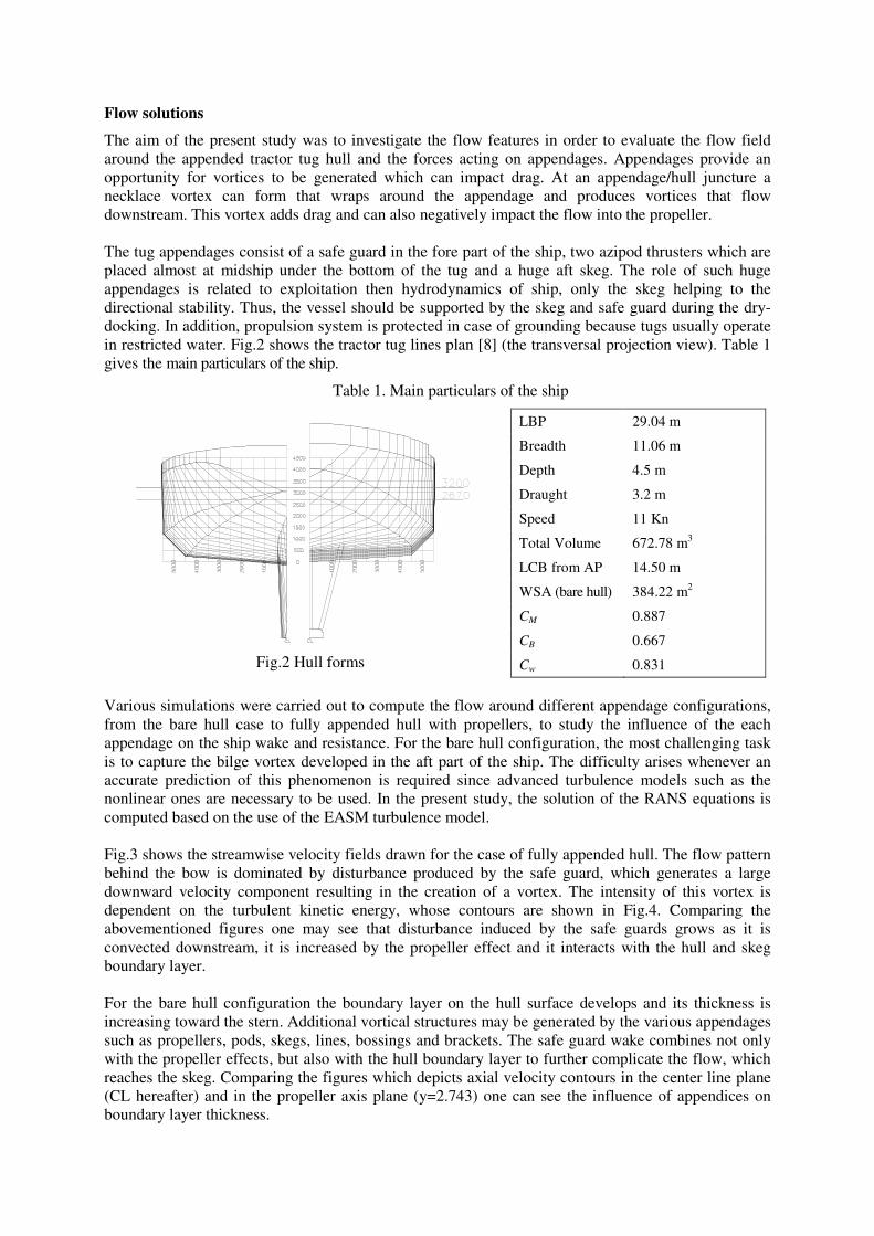
Flow solutions

The aim of the present study was to investigate the flow features in order to evaluate the flow field

around the appended tractor tug hull and the forces acting on appendages. Appendages provide an

opportunity for vortices to be generated which can impact drag. At an appendage/hull juncture a

necklace vortex can form that wraps around the appendage and produces vortices that flow

downstream. This vortex adds drag and can also negatively impact the flow into the propeller.

The tug appendages consist of a safe guard in the fore part of the ship, two azipod thrusters which are

placed almost at midship under the bottom of the tug and a huge aft skeg. The role of such huge

appendages is related to exploitation then hydrodynamics of ship, only the skeg helping to the

directional stability. Thus, the vessel should be supported by the skeg and safe guard during the dry-

docking. In addition, propulsion system is protected in case of grounding because tugs usually operate

in restricted water. Fig.2 shows the tractor tug lines plan [8] (the transversal projection view). Table 1

gives the main particulars of the ship.

Table 1. Main particulars of the ship

LBP 29.04 m

Breadth 11.06 m

Depth 4.5 m

Draught 3.2 m

Speed 11 Kn

Total Volume 672.78 m3

LCB from AP 14.50 m

WSA (bare hull) 384.22 m2

CM 0.887

CB 0.667

Fig.2 Hull forms Cw 0.831

Various simulations were carried out to compute the flow around different appendage configurations,

from the bare hull case to fully appended hull with propellers, to study the influence of the each

appendage on the ship wake and resistance. For the bare hull configuration, the most challenging task

is to capture the bilge vortex developed in the aft part of the ship. The difficulty arises whenever an

accurate prediction of this phenomenon is required since advanced turbulence models such as the

nonlinear ones are necessary to be used. In the present study, the solution of the RANS equations is

computed based on the use of the EASM turbulence model.

Fig.3 shows the streamwise velocity fields drawn for the case of fully appended hull. The flow pattern

behind the bow is dominated by disturbance produced by the safe guard, which generates a large

downward velocity component resulting in the creation of a vortex. The intensity of this vortex is

dependent on the turbulent kinetic energy, whose contours are shown in Fig.4. Comparing the

abovementioned figures one may see that disturbance induced by the safe guards grows as it is

convected downstream, it is increased by the propeller effect and it interacts with the hull and skeg

boundary layer.

For the bare hull configuration the boundary layer on the hull surface develops and its thickness is

increasing toward the stern. Additional vortical structures may be generated by the various appendages

such as propellers, pods, skegs, lines, bossings and brackets. The safe guard wake combines not only

with the propeller effects, but also with the hull boundary layer to further complicate the flow, which

reaches the skeg. Comparing the figures which depicts axial velocity contours in the center line plane

(CL hereafter) and in the propeller axis plane (y=2.743) one can see the influence of appendices on

boundary layer thickness.

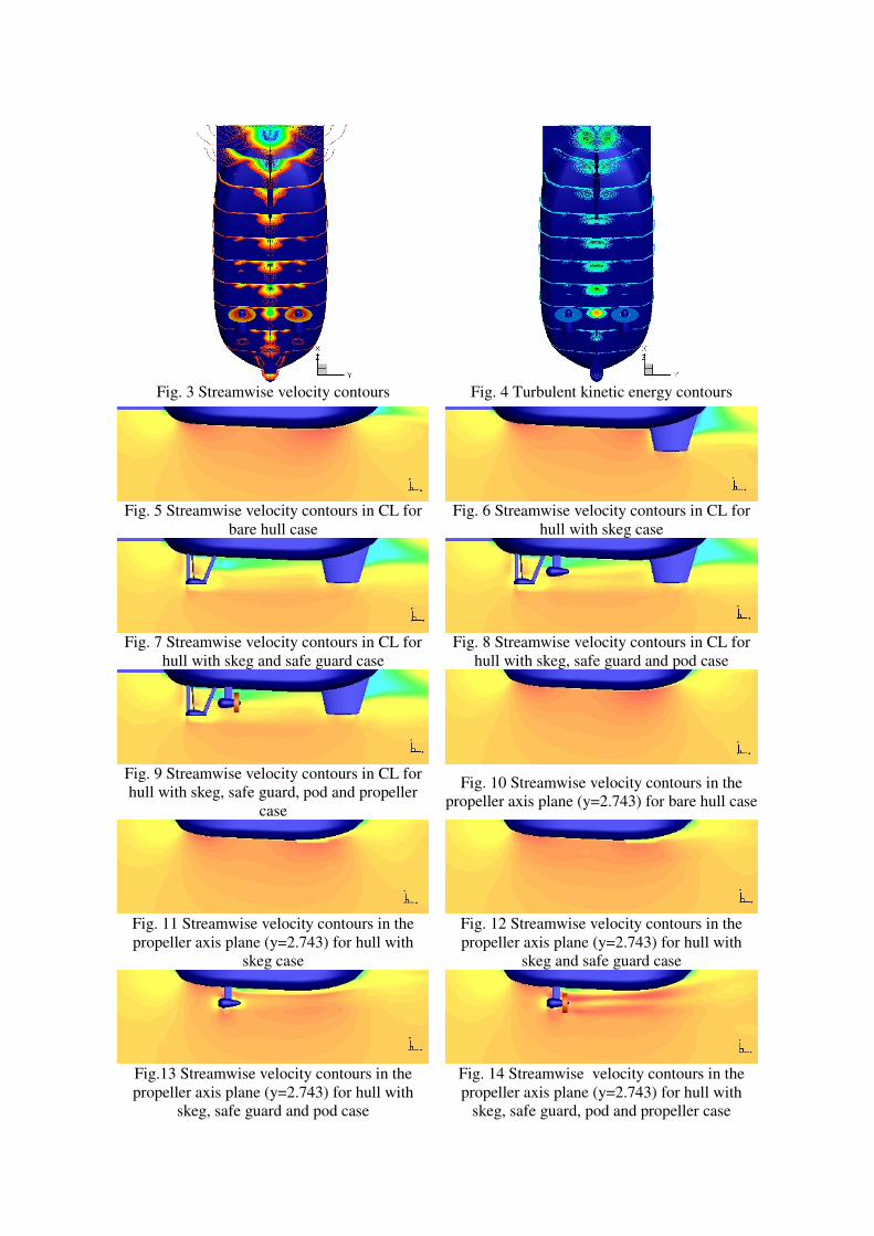
Fig. 3 Streamwise velocity contours Fig. 4 Turbulent kinetic energy contours

Fig. 5 Streamwise velocity contours in CL for

bare hull case

Fig. 6 Streamwise velocity contours in CL for

hull with skeg case

Fig. 7 Streamwise velocity contours in CL for

hull with skeg and safe guard case

Fig. 8 Streamwise velocity contours in CL for

hull with skeg, safe guard and pod case

Fig. 9 Streamwise velocity contours in CL for

hull with skeg, safe guard, pod and propeller

case

Fig. 10 Streamwise velocity contours in the

propeller axis plane (y=2.743) for bare hull case

Fig. 11 Streamwise velocity contours in the

propeller axis plane (y=2.743) for hull with

skeg case

Fig. 12 Streamwise velocity contours in the

propeller axis plane (y=2.743) for hull with

skeg and safe guard case

Fig.13 Streamwise velocity contours in the

propeller axis plane (y=2.743) for hull with

skeg, safe guard and pod case

Fig. 14 Streamwise velocity contours in the

propeller axis plane (y=2.743) for hull with

skeg, safe guard, pod and propeller case

The influence of the operating propeller on the flow field around the ship hull is obviously shown in

Fig. 14, the acceleration that the flow undergoes when passing through the propeller is clear, as well as

the suction effect on the pod surface. The analysis of flow field predictions reveals that the boundary

layer generated by the ship hull is correctly described.

Concluding remarks

The computational analysis of the flow field around a tractor tug vessel using a SHIPFLOW RANS

code has been presented. Various simulations were carried out to compute the flow around different

appendage configurations, from the bare hull case to fully appended hull with propellers, to study the

influence of the each appendage on the ship wake and resistance.

Acknowledgments

The reported research could not be possible without the generosity of the CNCSIS for the financial

support provided through the Grant 790/2008, for which it is greatly acknowledged. Special thank

goes to FLOWTECH International AB for supporting the attendance of NuTTS.

References

[1] Zhang, D.H., Broberg, L., Larsson, L., Dyne, G., A Method for Computing Stern Flows with an

Operating Propeller, RINA Transactions, 134, 1992.

[2 ]Zhou, L., Zhao, F., An integrated method for computing the internal and external viscous flow field

around the ducted propulsor behind an axisymmetric body, Proceedings of the 20th ONR Symposium,

pp. 1011–1020, 1994

[3] Steger, J.L., The Chimera Method of Flow Simulation, Workshop on Applied CFD, University of

Tennessee Space Institute, 1991

[4] Steger, J.L., Dougherty, F.C., Benek, J., A Chimera Grid Scheme Advanced in Grid Generation,

ASME FED, Vol. 5, pp.59-69, 1983.

[5] Wang, Z., A Fully Conservative Interface Algorithm for Overlapped Grids, J. Comput. Phys, 122,

pp. 96-106, 1995

[6] Regnström, B., Broberg L., Larsson, L., Overlapping composite grids for ship stern flow

calculations, MARNET-CFD First Workshop, Barcelona, 1999

[7] *** ShipFlow User’s Manual, FlowTech International, 2003

[8] Obreja, D., Popescu, G., Pacuraru, F., Resistance Tests Report. Tractor Tug, Research Project No.

344/2004, “Dunarea de Jos” University of Galati, 2004.

6DOF RANS Simulations of Floating and Submerged Bodies using OpenFOAM

Eric Paterson, David Boger, Gina Casadei, Scott Miller, Penn State University, egp11@psu.edu

Hrvoje Jasak, Wikki Ltd

Current status on the use of OpenFOAM (open source Field-Operation and Manipulation) for simulation

of floating and submerged bodies in waves will be reported. An OpenFOAM solver, rasInterDyMFoam,

has been developed which couples the 6DOF trajectory, mesh motion, hydrostatics, and hydrodynamics to

achieve transient simulations appropriate for seakeeping, maneuvering, and wave-impact modeling. 6DOF

motion is computed using quaternion formulation of the equations of motion and mesh motion is

accommodated using tet FEM, GGI, and overset-grid techniques. Hydrostatic forces are computed through

direct integration of the total pressure field, and hydrodynamics are computed using the Navier-Stokes

equations with both RANS and hybrid RANS/LES turbulence models. Examples will be presented and

discussed.

Accurate capture of rudder-propeller interaction using

a coupled blade element momentum-RANS approach

Alexander Phillips∗, Maaten Furlong∗∗ and Stephen R Turnock∗

*Fluid-Structure Interaction Research Group, School of Engineering Sciences, University of Southampton,Highfield, Southampton SO17 1BJ, UK

**National Oceanography Centre, Southampton, European Way, Southampton, SO14 3ZH, UK

Corresponding author’s email : abp@soton.ac.uk

1 Introduction

Ship rudders are almost always placed downstream ofthe propeller so they can take advantage of the in-creased local velocity due to the presence of the pro-peller race. The methods discussed in this paper repli-cate the flow integrated effects of the propeller whichgenerates an accelerated and swirled onset flow ontothe rudder. As long as the radial variation in axialand tangential momentum (including hull and rudderinteraction effects) generated by the propeller are in-cluded, then the influence of the unsteady propellerflow can be removed and ’steady’ calculations per-formed to evaluate propeller rudder interaction.

Three different body force propeller models will beconsidered and numerical results will be comparedwith experiments by Molland and Turnock [1, 2, 3],using the modified Wageningen B4.40 propeller andRudder No.2.

2 Theoretical Approach

The flow around a rotating propeller is a highly com-plex 3D transient flow, therefore modelling a rotatingpropeller explicitly leads to significant computationalcost within a RANS simulation. This is due to the highmesh resolution required around the blade to capturethe flow features and the small time steps requiredto capture the transients flow features. For work notconcentrating on the propeller itself but rather the in-teraction of the propeller hull and rudder system itmay not be vital to capture all aspects of the pro-peller flow, however providing a representative modelof the velocity field is extremely important. Basedon this assumption several body force propeller mod-els have been proposed to reduce computational cost,which facilitate self propelled simulations.

When using a body force model the propeller is notphysically represented by its geometry. Instead theeffect of the propeller on the flow is included by rep-resenting the propeller as a series of axial and mo-mentum source terms, fbx and fbθ respectively, whichare distributed over the propeller disc, these induce anaxial and swirl acceleration in the fluid.

In order to implement a body force propeller modelin a RANS simulation both the magnitude and dis-tribution of the thrust, T , and torque, Q, induced bythe propeller needs to be determined. Three differentbodyforce models will be considered:-

1. Uniform thrust distribution with no torque,equivalent to an actuator disc applied over a finitethickness.

2. Hough and Ordway prescribed thrust and torquedistribution.

3. Thrust and torque magnitude and distribu-tion from Blade Element Momentum Theory(BEMT).

Typical velocity profiles available in the literature,[4], show that the velocity in the radial direction is anorder of magnitude smaller than the tangential veloc-ity component, hence it is assumed valid to not modelthe blade local induced radial velocity changes. Radialvelocity changes due to contraction of the slipstreamare incorporated by the RANS equations in order tomaintain continuity.

2.1 Uniform Thrust Distribution - RANS-UT

A uniform distribution of thrust is assumed and thetorque is neglected, equivalent to momentum theory.The axial momentum source term is given by:-

fbx =T

∆xπ(R2p −R2

h), (1)

while the tangential momentum term is given by:-

fbθ = 0, (2)

where ∆x is the thickness of the propeller subdomainand Rh and Rp are the radius of the hub and propellerrespectfully. The magnitude of T must be provided bysome other means, either experimental, based on openwater data or from numerical predictions.

2.2 Hough and Ordway Thrust and Torque Distribu-tion - RANS-HO

The radial distribution of thrust and torque is basedon the [5] circulation distribution which has zero load-ing on the tip and root. The distribution was shown toclosely match Goldstein’s optimum distribution. Cou-pling this distribution with a RANS simulation wasproposed by [6], and is implemented in CFDSHIP-IOWA, [7]. The non-dimensional thrust distributionfb′x and torque distribution fb′θ are given by:-

fb′x = Axr∗√

1− r∗ (3)

fb′θ = Aθr∗√

1− r∗

(1− Yh)r∗ + Yh(4)

Where:

Ax =CT

∆x

105

16(4 + 3Yh)(1− Yh)(5)

Aθ =KQ

∆xJ2.

105

π(4 + 3Yh)(1− Yh)(6)

where the non dimensional radius is defined as r∗ =

(Y − Yh)/(1− Yh), Y = r/Rp and Yh = Rh/Rp.

CT =T

1/2ρU2aπR2

p

=KT

π/8J2(7)

For uniform propeller inflow such as that expe-rienced by a propeller rudder system operating infreestream, [8] demonstrated that the use of this thrustand torque distribution lead to good estimates of rud-der forces.

2.3 Blade Element Momentum Theory, Thrust andTorque Magnitude and Distribution Prediction -RANS-BEMT

The thrust and torque distribution will vary depend-ing on the geometry of the propeller, rpm and advancevelocity. To incorporate these variations the thrustand torque magnitude and distribution are calculatedusing an existing Blade Element Momentum Theorycode [9].

In order to capture the radial and circumferentialvariation in propeller inflow conditions due to blockageeffects from the rudder, the propeller plane is subdi-vided into for 360 discrete zones (10 radial divisions, 36circumferential divisions). The BEMT code is calledfor each of these locations to determine the local KT

and KQ based on local inflow conditions. For each nodein the propeller subdomain, the radial distance is cal-culated and the local thrust and torque magnitudesare interpolated from the distribution derived from theBEMT code. Further details of this approach may befound in [10, 11, 12].

3 Experimental Data

Wind tunnel tests performed by Molland and Turnockin the University of Southampton 3.5×2.5m RJ MitchellWind Tunnel [13]. The experimental set up is shownin Figure 1, it comprises of a 1m span, 1.5 geomet-ric aspect ratio rectangular planform rudder, and arepresentative 0.8m diameter propeller based on theWageningen B4.40 series placed at X/D = 0.39. Furtherdetails of the experiment can be found in [3].

4 Numerical Model

The motion of the fluid is modelled using the incom-pressible (8), isothermal Reynolds Averaged NavierStokes (RANS) equations (9) in order to determinethe cartesian flow field (ui = u, v, w) and pressure (p) ofthe water around the hull:

Figure 1: Isometric view of experimental setup, [1]

∂Ui

∂xi= 0 (8)

ρ∂Ui

∂t+ ρ

∂UiUj

∂xj

= −∂P

∂xi

+∂

∂xj

(µ

∂Ui

∂xj

+∂Uj

∂xi

!)− ρ

∂u′iu′j

∂xj

+ fi

(9)The influence of turbulence on the mean flow is rep-

resented in equation (9) by the Reynolds stress tensor(ρu′iu′j).

Closure of the RANS equations is achieved for thiscase using the Shear Stress Transport (SST) modeleddy viscosity turbulence closure model developed by[14]. SST is a two zone model that blends a variantof the k − ω model in the inner boundary layer with atransformed version of the k− ε in the outer boundarylayer and away from the wall. Previous investigationsfor Ship flows have shown it is better able to repli-cate the flow around ship hull forms than either zeroequation models or the k− ε model, notably in captur-ing hooks in the wake contours at the propeller plane,[15].

Simulations are performed using ANSYS CFX, acommercial, fully implicit finite volume code, usinga variation of the SIMPLE (Semi-Implicit Method forPressure Linked Equations) algorithm for momentum-pressure decoupling. Details of the computationalmodel are provided in Table 1.

4.1 Model Domain and Boundary Conditions

The lateral dimensions were matched to those of theRJ Mitchell wind tunnel, with the domain extending2.8 chord lengths upstream of the rudder and 8 chordlengths downstream. The following boundary condi-tions were applied:

• Inlet - Dirchlet boundary condition, nominal in-flow velocity 10 m/s, with representative 70mmthick boundary layer distribution applied overfloor, turbulence intensity 0.002, eddy lengthscale 0.01m.

• Outlet - Neumann boundary condition, velocityand pressure gradients set to zero, with a zerorelative pressure

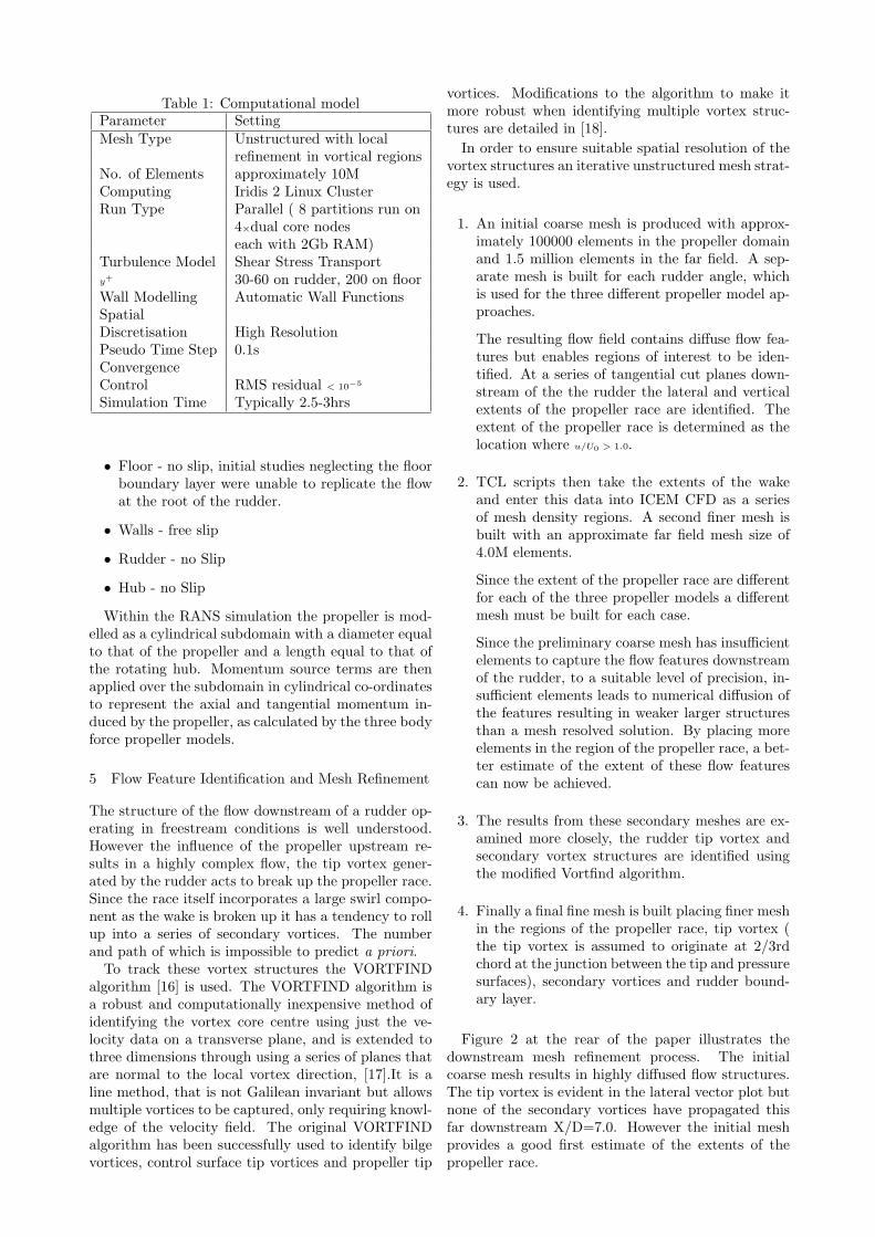
Table 1: Computational modelParameter SettingMesh Type Unstructured with local

refinement in vortical regionsNo. of Elements approximately 10MComputing Iridis 2 Linux ClusterRun Type Parallel ( 8 partitions run on

4×dual core nodeseach with 2Gb RAM)

Turbulence Model Shear Stress Transporty+ 30-60 on rudder, 200 on floorWall Modelling Automatic Wall FunctionsSpatialDiscretisation High ResolutionPseudo Time Step 0.1sConvergenceControl RMS residual < 10−5

Simulation Time Typically 2.5-3hrs

• Floor - no slip, initial studies neglecting the floorboundary layer were unable to replicate the flowat the root of the rudder.

• Walls - free slip

• Rudder - no Slip

• Hub - no Slip

Within the RANS simulation the propeller is mod-elled as a cylindrical subdomain with a diameter equalto that of the propeller and a length equal to that ofthe rotating hub. Momentum source terms are thenapplied over the subdomain in cylindrical co-ordinatesto represent the axial and tangential momentum in-duced by the propeller, as calculated by the three bodyforce propeller models.

5 Flow Feature Identification and Mesh Refinement

The structure of the flow downstream of a rudder op-erating in freestream conditions is well understood.However the influence of the propeller upstream re-sults in a highly complex flow, the tip vortex gener-ated by the rudder acts to break up the propeller race.Since the race itself incorporates a large swirl compo-nent as the wake is broken up it has a tendency to rollup into a series of secondary vortices. The numberand path of which is impossible to predict a priori.

To track these vortex structures the VORTFINDalgorithm [16] is used. The VORTFIND algorithm isa robust and computationally inexpensive method ofidentifying the vortex core centre using just the ve-locity data on a transverse plane, and is extended tothree dimensions through using a series of planes thatare normal to the local vortex direction, [17].It is aline method, that is not Galilean invariant but allowsmultiple vortices to be captured, only requiring knowl-edge of the velocity field. The original VORTFINDalgorithm has been successfully used to identify bilgevortices, control surface tip vortices and propeller tip

vortices. Modifications to the algorithm to make itmore robust when identifying multiple vortex struc-tures are detailed in [18].

In order to ensure suitable spatial resolution of thevortex structures an iterative unstructured mesh strat-egy is used.

1. An initial coarse mesh is produced with approx-imately 100000 elements in the propeller domainand 1.5 million elements in the far field. A sep-arate mesh is built for each rudder angle, whichis used for the three different propeller model ap-proaches.

The resulting flow field contains diffuse flow fea-tures but enables regions of interest to be iden-tified. At a series of tangential cut planes down-stream of the the rudder the lateral and verticalextents of the propeller race are identified. Theextent of the propeller race is determined as thelocation where u/U0 > 1.0.

2. TCL scripts then take the extents of the wakeand enter this data into ICEM CFD as a seriesof mesh density regions. A second finer mesh isbuilt with an approximate far field mesh size of4.0M elements.

Since the extent of the propeller race are differentfor each of the three propeller models a differentmesh must be built for each case.

Since the preliminary coarse mesh has insufficientelements to capture the flow features downstreamof the rudder, to a suitable level of precision, in-sufficient elements leads to numerical diffusion ofthe features resulting in weaker larger structuresthan a mesh resolved solution. By placing moreelements in the region of the propeller race, a bet-ter estimate of the extent of these flow featurescan now be achieved.

3. The results from these secondary meshes are ex-amined more closely, the rudder tip vortex andsecondary vortex structures are identified usingthe modified Vortfind algorithm.

4. Finally a final fine mesh is built placing finer meshin the regions of the propeller race, tip vortex (the tip vortex is assumed to originate at 2/3rdchord at the junction between the tip and pressuresurfaces), secondary vortices and rudder bound-ary layer.

Figure 2 at the rear of the paper illustrates thedownstream mesh refinement process. The initialcoarse mesh results in highly diffused flow structures.The tip vortex is evident in the lateral vector plot butnone of the secondary vortices have propagated thisfar downstream X/D=7.0. However the initial meshprovides a good first estimate of the extents of thepropeller race.

6 Results and Discussion

Preliminary results are presented below for a propelleroperating condition of J = 0.35, further smoothing of themesh is required in the mesh transition region betweenthe floor boundary layer and rudder boundary layer.Some poor quality elements in this region are leadingto numerical instabilities, visible in the rudder surfacepressure plots.

6.1 Lift and Drag Data

Figure 3 and 4 compares the experimental and nu-merical lift and drag respectively. Results are alsopresented from [8] who performed similar numericalsimulations using the CFDSHIP-IOWA code using aHough and Ordway thrust and torque distribution,and from [19] using the 3D panel code Palisupan, [20].Table 2 compares values of dCL/dδ and δ0.

By neglecting the influence of propeller inducedswirl on the fluid, the RANS-UT model produces sym-metric results at ±10 and the rudder neutral angle isat 0. However the magnitude of the lift results pro-vide good indicative results, the gradient of the liftslope is within 10% of mean experimental value. Forthis case the drag experienced by the rudder is signif-icantly greater than the experimental results for theRANS-UT model, this is due to the influence of swirlon local incidence angle. Experimental results showa decrease in rudder drag with increasing propellerthrust loading.

The RANS-HO and RANS-BEMT approaches showvery good correlation with the experiential lift resultsin terms of both neutral rudder angle, δ0, and lift slopegradient. The asymmetry due to the swirl action ofthe propeller is well reproduced.

Table 2: Propeller detailsData Set dCL

dδδ0

Molland and Turnock SS46 0.132 0.093Molland and Turnock SS90 0.136 0.526

Turnock (1993) 0.140 1.376Simonseen 2000 0.147 1.383

RANS-UT 0.124 0.000RANS-HO 0.136 0.255

RANS-BEMT 0.142 0.264

6.2 Rudder Surface Pressure

The ability of the three propeller models to replicatethe downstream wake of a propeller can be inferred bytheir ability to replicate the correct pressure distribu-tion on the rudder surface.

Examining the Cp =P−P01/2ρU2

0distribution for a

freestream rudder, you observe a Cp value of 1.0 atthe stagnation point, where the flow velocity drops tozero. For a rudder downstream of a propeller the in-flow velocity is greater than the freestream velocity,hence the stagnation pressure is higher leading to CP

Figure 3: Rudder 2 - CL performance J=0.35

Figure 4: Rudder 2 - CD performance J=0.35

values in excess of 1. Accurate prediction of stagna-tion CP values implies the correct inflow velocity hasbeen generated by the propeller model.

Figure 5 compares experimental and numerical pres-sure distributions at a series of span locations fromroot to tip for a rudder angle of δ = 0.

The RANS-UT model experiences a symmetric pres-sure distribution down both sides of the rudder instark contrast to the more complex models and the ex-perimental data. Both the RANS-BEMT and RANS-HO models relatively well reproduce the pressure dis-tribution for most of the locations considered showingclear improvement over the RANS-UT approach.

Both the RANS-BEMT and RANS-HO approachesare relatively well able to replicate the pressure distri-bution at incidence angles of both 10 and -10 degrees.Since the swirl imparted swirl direction is constant inboth cases the resulting pressure fields are substan-tially different and this is reproduced in the numericalresults.

7 Conclusions

The methods discussed in this paper make use of theflow integrated effects of the propeller which gener-ates an accelerated and swirled onset flow onto therudder. As long as the radial variation in axial andtangential momentum generated by the propeller areincluded, then the influence of the unsteady propellerflow can be removed and ’steady’ calculations per-formed to evaluate the influence of the propeller onthe rudder.

The uniform thrust approach which neglects swirlresults in adequate prediction of rudder lift but is un-able to well predict the rudder drag.

The prescribed thrust and torque distribution ofHough and Ordway and the coupled RANS-BEMTapproach are better able to recreate the wake down-stream of the propeller and the resulting rudder loadsand surface pressure distribution compare favourablywith the experimental data.

This RANS-HO approach is only useful to investi-gate the influence of the propeller on the rudder. In-teraction effects due to the rudder on the propellerare not captured, and neither would the influence ofthe hull on the propeller inflow conditions. The block-age effects of the rudder or influence of non uniforminflow into the propeller can be achieved using thecoupled RANS-BEMT approach described, making itmore suitable for cases involving hull, propeller andrudder such as self propulsion simulations.

Acknowledgements

Mr Phillips’ PhD studentship is jointly financed bythe School of Engineering Science and the NationalOceanography Centre, Southampton.

References

[1] A. F. Molland and S. R. Turnock. Wind tunnel investigation ofthe influence of propeller loading on ship rudder performance.Technical report, Ship Science Report No. 46, 1991.

[2] A.F. Molland and S.R. Turnock. Wind tunnel tests on the ef-fect of a ship hull on rudder-propeller performance at differentdrift angles. Technical report, University of Southampton ShipScience Report No. 76, May 1995.

[3] A.F. Molland and S.R. Turnock. Marine Rudders and ControlSurfaces. Butterworth-Heinemann, 2007.

[4] C. Kee, G.A. Hamill, W-H. Lam, and P.W. Wilson. Inves-tigation of the velocity distributions within a ships propellerwash. In Proceedings of the Sixteenth (2006) InternationalOffshore and Polar Engineering Conference San Francisco,California, USA,, May 28-June 2, 2006.

[5] G. R. Hough and D. E. Ordway. The generalised actuator disc.Developments in Theoretical and Applied Mechanics, 2:317–336, 1965.

[6] F. Stern, H. T. Kim, N. M. Patel, and H. C. Chen. A viscous-flow approach to the computation of propeller-hull interaction.Journal of Ship Research, 32:246–262, 1988.

[7] E. G. Paterson, R.V. Wlison, and F. Stern. General purposeparrallel unsteady rans ship hydrodynamics code CFDSHIP-IOWA. Technical report, Iowa Institute of Hydraulic Research,The University of Iowa, 2003.

[8] C. D. Simonsen. Rudder, Propeller and Hull Interaction byRANS. PhD thesis, Department of Naval Architecture andOffshore Engineering, 2000.

[9] A. F. Molland and S. R. Turnock. A compact computationalmethod for predicting forces on a rudder in a propeller slip-stream. In Transactions of RINA, volume 138, pages 59–71,1996.

[10] S.R Turnock, A.B. Phillips, and M Furlong. Urans simulationsof static drift and dynamic manoeuvres of the kvlcc2 tanker.In SIMMAN International Manoeuvring Workshop, Copen-hagen, April 2008.

[11] A.B. Phillips, M. Furlong, and S.R. Turnock. Comparisons ofcfd simulations and in-service data for the self propelled per-formance of an autonomous underwater vehicle. In 27th Sym-posium on Naval Hydrodynamics Seoul, Korea, 5-10 October2008.

[12] A.B. Phillips, S.R Turnock, and M. Furlong. Simulation of aself-propelled ship using a blade element momentum propellermodel and rans. Submitted to Journal of Ocean Engineering,2009.

[13] WWW1. http : //www.windtunnel.soton.ac.uk/index.html.World Wide Web, 2009.

[14] F.R. Menter. Two-equation eddy-viscosity turbulence modelsfor engineering applications. AIAA Journal, 32(8):1598 – 605,1994.

[15] L. Larsson, F. Stern, and V. Bertram. Benchmarking of com-putational fluid dynamics for ship flows: The gothenburg 2000workshop. Journal of Ship Rese, 47:63–81(19), 1 March 2003.

[16] R. J. Pemberton, S. R. Turnock, T. J. Dodd, and E. Rogers.A novel method for identifying vortical structures. Journal ofFluids and Structures, 16:1051–1057, 2002.

[17] C. Pashias. PROPELLER TIP VORTEX SIMULATION US-ING ADAPTIVE GRID REFINEMENT BASED ON FLOWFEATURE IDENTIFICATION. PhD thesis, University ofSouthampton, 2005.

[18] A. B. Phillips. Cost effective hydrodynamic design of Au-tonomous Underwater Vehicles. PhD thesis, School of Engi-neering Sciences, University of Southampton, to be submitted2009.

[19] S.R. Turnock. Prediction of ship rudder-propeller interactionusing parallel computations and wind tunnel measurements.PhD thesis, University of Southampton, Ship Science, 1993.

[20] S.R. Turnock. Technical manual and user guide for the sur-face panel code: Palisupan. Technical report, University ofSouthampton, Southampton, UK (Ship Science Reports, 100),1997.

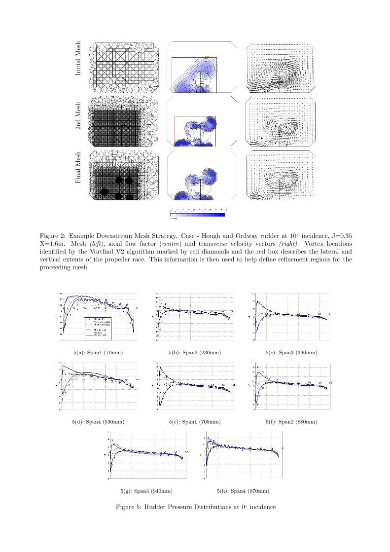
Init

ialM

esh

2nd

Mes

hFin

alM

esh

Figure 2: Example Downstream Mesh Strategy. Case - Hough and Ordway rudder at 10 incidence, J=0.35X=1.6m. Mesh (left), axial flow factor (centre) and transverse velocity vectors (right). Vortex locationsidentified by the Vortfind V2 algorithm marked by red diamonds and the red box describes the lateral andvertical extents of the propeller race. This information is then used to help define refinement regions for theproceeding mesh

5(a): Span1 (70mm) 5(b): Span2 (230mm) 5(c): Span3 (390mm)

5(d): Span4 (530mm) 5(e): Span1 (705mm) 5(f): Span2 (880mm)

5(g): Span3 (940mm) 5(h): Span4 (970mm)

Figure 5: Rudder Pressure Distributions at 0 incidence

Multi-objective Optimization of a Tanker Afterbody

using PARNASSOS

Auke van der Ploeg, MARIN, Wageningen/NL, A.v.d.Ploeg@MARIN.NL

Martin Hoekstra, MARIN, Wageningen/NL, M.Hoekstra@MARIN.NL

Ship resistance and propulsion are principal aspects for the fuel efficiency of maritime transport.

Modern CFD techniques allow a further improvement of that efficiency by precisely predicting resis-

tance and scale effects, by computational optimization for minimum resistance or power, and by un-

derstanding and limiting propeller cavitation to shift the constraints on efficiency. In the European

project VIRTUE, an EC-funded project under the 6th Framework program, 22 institutes and universi-

ties have cooperated in carrying out research to advance the role of CFD in ship hydrodynamics and

design. In the Resistance and Propulsion work package, significant improvements were made in the

quality of resistance and wave making computations and in the computation of scale effects [2].

Based on this, procedures for multi-objective optimization of ship hulls were developed. The work

culminated in a VIRTUE workshop in which 5 participants optimized the same tanker afterbody with

respect to both resistance and wake field quality. Main dimensions and displacement were kept un-

changed, and ‘hard points’ guaranteed sufficient room for machinery. Each participant used his own

CAD system, hull form variation technique, RANS code and optimizer, and finally submitted an op-

timized hull form, which was evaluated by cross computations by other participants. For the most

promising hull form, a model was built and measurements were performed.

The RANS code we use is PARNASSOS which has been developed and frequently applied by MARIN

and IST [1]. It is dedicated to the prediction of the steady turbulent flow around ship hulls and solves

the discretised Reynolds-averaged Navier-Stokes equations for steady incompressible flow. Various

eddy-viscosity turbulence models are available. For this optimization exercise we use the standard k-

ω SST turbulence model without corrections. Structured multi block body-fitted grids are used, usu-

ally of H-O topology. A finite-difference discretisation is used, with second and third-order schemes

for the various terms. As part of an optimization exercise, in general a large number of RANS compu-

tations has to be done. An efficient solution technique is therefore imperative. PARNASSOS solves the

momentum and continuity equations in their original, fully coupled form. Therefore, the continuity

equation need not be recast in a pressure correction or pressure Poisson equation, but can simply be

solved as it is. After discretisation and linearization, the three momentum equations and the continuity

equation give rise to a matrix equation containing 4*4 blocks, which is solved using preconditioned

GMRES. This fully coupled solution has been found to be robust and quite insensitive to the mesh

aspect ratio. The solution procedure exploits the character of the ship flow problem, which has a pre-

dominant flow direction. The equations are solved for subdomains that consist of several streamwise

stations at a time. All variables for a subdomain are solved simultaneously. The subdomains are ad-

dressed in a downstream sequence. This downstream marching sweep has to be repeated until conver-

gence in order to couple the subdomains and to take into account both the nonlinearity and the elliptic

character of the RANS equations. More details about the solution strategy can be found in [3]. CPU

and memory requirements of the PARNASSOS code are quite modest compared to most other methods;

e.g. a double-body computation for a single-screw ship on a mesh with 2M cells takes about 2 hours

CPU time on a single-processor PC.

As mentioned before, only the aft part of the tanker was allowed to be changed. All participants used

double body, model-scale RANS computations without a propeller model. Neither the main dimen-

sions (LPP =320 m, T=21 m, B=60 m) nor the Reynolds number (6.5⋅107) were allowed to be changed.

In addition, the displacement was not allowed to decrease and the position of the propeller was fixed.

To guarantee sufficient space for machinery, the dashed lines in Fig.1 had to stay inside the optimized

hull for any proposed variant from station 1.5125 to further ahead.

Fig.1: Frames afterbody of the initial tanker

The two objective functions were the viscous resistance RT and a wake object function (WOF). The

latter can be interpreted as a ‘non-uniformity of wake field / nominal wake’. It is defined as

in which where VS is the velocity relative to the ship, non-dimensionalized with the

ships speed. The numerator considers RMS of deviations from average velocity at radii 0.6…1.0

times the propeller radius. The sum over φ is taken in circumferential direction in steps of 5°.

The systematic variations consisted of the following steps:

1. Define some basis hull forms. Any design experience can be used in this step, but oth-

erwise successive optimization cycles will give guidance: if the best results are found

on the border of the chosen design space, there is a clear indication in which direction

further changes should be made. 2. Use GMS merge to make combinations of these basis hull forms. The GMS merge tool has

been developed at MARIN and enables the generation of a special interpolation of some pre-

defined hull form variants in a very efficient way. This tool will be demonstrated during the

presentation.

3. The parameters of hull forms to be evaluated are defined to be the percentages of the respec-

tive basis hull forms. For example, if we start with 6 basis hull forms, we have a 5-

dimensional parameter space, and if we use steps of 33.3% to go from one hull form to the

next, we have a total of 45=1024 variants.

4. Do a RANS computation for each variant, with the grid for each hull form obtained from a

fully automatic grid generation procedure. An automatic procedure for grid generation has

been developed that allows strong modifications of the hull form. Tools for distribution of the

work over a network of PCs permit several hundreds of RANS-computations in only a couple

of hours.

Before deciding which grid density to use, it has been checked that the trends in the objective func-

tions do not change significantly with grid refinement. This is illustrated in Fig.2, which compares the

wake fields for the initial tanker in the propeller plane obtained with two grid densities. It appears that

the wake field hardly changes with grid refinement. The effect of grid refinement on the computed

Pareto front will be illustrated below.

∑ ∑∑ ∑ ∑=

°

°==

°

°=

°

°=

−

0.1

6.0

355

0

0.1

6.0

355

0

2355

0

),(72

1),(

72

1),(

72

1

r

total

r

totaltotal rWrWrWϕϕ ϕ

ϕϕϕ

21 Stotal VW −=

In addition, the computed trends should not be influenced by the stop criterion in the RANS computa-

tion. Fig.3 demonstrates a study on the effect of different stop criteria for a simple one-parameter

study (a variation between two basis hull forms). The RANS computation was stopped when the

maximum difference in the pressure coefficient (dcp) was below a given value. Only for dcp < 10-5

the influence of incomplete convergence on the results is negligible.

Modification

10

00

xC

p

0 20 40 60 80 100

1.34

1.36

1.38

1.4

1.42

Max(dcp)<10-3

Max(dcp)<10-4

Max(dcp)<10-5

Max(dcp)<10-6

Fig.2: Grid refinement study Fig.3: Effect stop criterion RANS computation

In several parametric studies we have thus done some 1500 evaluations of hull forms. For all these

results, Fig.4 shows the decrease of the resistance relative to the initial hull form on the vertical axis,

the decrease of the Wake Object Function (WOF) on the horizontal axis. Each point gives the com-

puted values for one hull form variant: each red triangle shows the computed value of a RANS com-

putation on a coarse grid, and each black box a result obtained on a refined grid. There is a clear enve-

lope, a ‘Pareto front’, that indicates the best that can be achieved. Of course, eventually one has to

choose one variant on the Pareto front, thus making a compromise between both objectives. This front

is hardly influenced by the grid density, which lends much confidence to the results. For example, for

two hull forms (‘candidate 1’ and ‘candidate 2’), the results obtained on the coarse grid and fine grid

are indicated in Fig.4. It appears that grid refinement results in a small shift along the Pareto front.

Fig.4: Computed Pareto front

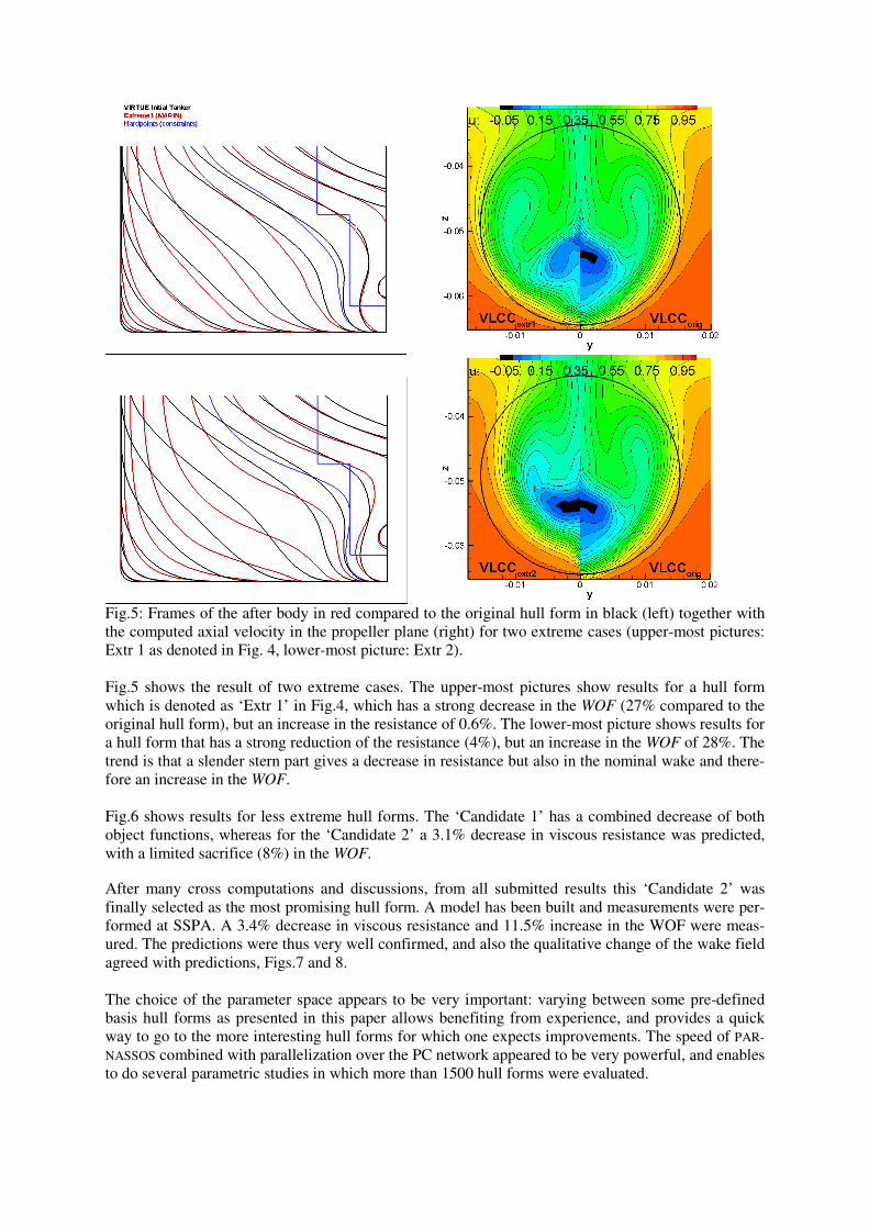
Fig.5: Frames of the after body in red compared to the original hull form in black (left) together with

the computed axial velocity in the propeller plane (right) for two extreme cases (upper-most pictures:

Extr 1 as denoted in Fig. 4, lower-most picture: Extr 2).

Fig.5 shows the result of two extreme cases. The upper-most pictures show results for a hull form

which is denoted as ‘Extr 1’ in Fig.4, which has a strong decrease in the WOF (27% compared to the

original hull form), but an increase in the resistance of 0.6%. The lower-most picture shows results for

a hull form that has a strong reduction of the resistance (4%), but an increase in the WOF of 28%. The

trend is that a slender stern part gives a decrease in resistance but also in the nominal wake and there-

fore an increase in the WOF.

Fig.6 shows results for less extreme hull forms. The ‘Candidate 1’ has a combined decrease of both

object functions, whereas for the ‘Candidate 2’ a 3.1% decrease in viscous resistance was predicted,

with a limited sacrifice (8%) in the WOF.

After many cross computations and discussions, from all submitted results this ‘Candidate 2’ was

finally selected as the most promising hull form. A model has been built and measurements were per-

formed at SSPA. A 3.4% decrease in viscous resistance and 11.5% increase in the WOF were meas-

ured. The predictions were thus very well confirmed, and also the qualitative change of the wake field

agreed with predictions, Figs.7 and 8.

The choice of the parameter space appears to be very important: varying between some pre-defined

basis hull forms as presented in this paper allows benefiting from experience, and provides a quick

way to go to the more interesting hull forms for which one expects improvements. The speed of PAR-

NASSOS combined with parallelization over the PC network appeared to be very powerful, and enables

to do several parametric studies in which more than 1500 hull forms were evaluated.

Fig.6: Frames of the after body in red compared to the original hull form in black (left) together with

the computed axial velocity in the propeller plane (right) for two hull forms (upper-most pictures:

Candidate 1 as denoted in Fig.4, lower-most picture: Candidate 2).

Fig. 7: Measured total wake (measurements Fig.8: Computed total wake.

performed at SSPA) Left: Candidate 2.

Left: Candidate 2. Right: initial hull form

Right: initial hull form

In this way, a clear Pareto front could be computed, and it could be checked that the grid dependence

on the Pareto front is very limited. A compromise is required between decreasing RT and Wake Ob-

ject Function (WOF). Both the computed 3% decrease in resistance and the computed trends in the

wake field have been confirmed by measurements.

From some systematic variations (not presented in this paper) it appeared that a reduction of the resis-

tance of more than 5% is possible, but this almost doubles the WOF. For practical applications how-

ever, a decrease in the resistance is probably more important than a decrease in the WOF, because it is

very hard to find a definition of the wake object function that truly reflects the possibilities for propel-

ler designers to get to higher efficiencies, and at the same time takes into account the danger of (ero-

sive) cavitation. Doing the optimization directly for the hull form including a propeller model is there-

fore to be preferred. Another aspect is that the wake field and therefore the WOF strongly depend on

the Reynolds number. For practical applications it is therefore better to do optimizations directly at

full scale.

Acknowledgement

The research reported in this paper formed part of WP1 of the VIRTUE project, an Integrated Project

in the 6th Framework Program “Sustainable development, global change and ecosystems” under grant

516201 from the European Commission. This support is gratefully acknowledged.

References

1. Hoekstra, M., "Numerical simulation of ship stern flows with a space-marching Navier Stokes

method", Thesis, Technical University of Delft, October 1999.

2. Raven, H.C., van der Ploeg, A., Starke, A.R., and Eça, L., “Towards a CFD-based prediction of

ship performance -- Progress in predicting resistance and scale effects’’, Int. J. of Maritime En-

gineering, Trans. RINA Vol.150 – A4, 2008.

3. Van der Ploeg, A., Hoekstra, M., and Eça, L., “Combining accuracy and efficiency with robust-

ness in ship stern flow computation”, 23rd

Symp. Naval Hydrodynamics, Val de Reuil, France,

2000.

Simulating Ship Motions and Loads using OpenFOAM

Daniel Schmode, Volker Bertram, Germanischer Lloyd, daniel.schmode@gl-group.com

Matthias Tenzer, Universität Duisburg-Essen

The open source CFD package OpenFOAM can be used to simulate free-surface flows around ships

(interDyMFoam). It also provides a solver to integrate the equations of motions (EoM) for six degrees of

freedom (DoF) (sixDoFsolver). We have combined both features to an integrated solver, which can

simulate the 6DoF motions of floating structures.

OpenFOAM solves the (Reynolds averaged) Navier-Stokes equations. The free-surface modeling is based

on the Volume-of-Fluid (VOF) method. The domain is discretized using the Finite Volume Method

(FVM). Unstructured grids with arbitrary polygon cells are possible. The convection terms in the

momentum equation are approximated using a TVD limited linear second-order scheme. The pressure-

velocity coupling follows the PISO method. The VOF transport equations are discretized by a special

scheme, the explicit MULES scheme, ensuring a sharp interface between water and air. The sharpness of

the interface can be influenced via the parameter cGamma (see chapter PISO in fvSolutionDict).

Increasing cGamma makes the free surface interface crisper. The procedure for the integration of the

motion is formulated based on quaternions and thus avoids any singularities in the EoM (gimbal lock). It

is described in Shivarama and Fahrenthold (2004). The differential equations are discretized using the

Implicit Euler or Runge Kutta scheme. For floating bodies, the sum of fluid forces and mass forces must

be zero at all times. As the grid deformation and forces depend mutually on each other, explicit schemes

do not ensure equilibrium of forces. This may lead to instabilities in the numerical scheme, particularly for

large hydrodynamic masses. We employ a fully implicit scheme to couple ship motions and flow

simulations. To ensure numerical stability, the exciting forces are under-relaxed. Since the PISO scheme

for pressure-velocity coupling does not require outer iterations, iterations for grid deformation / force

determination were introduced. At the end of each grid iteration, the force equilibrium (fluid forces = mass

forces) is checked. The normalized difference between fluid and mass forces serves as criterion to stop the

grid iteration. Since the first grid deformation can be predicted well based on the previous time steps, the

approach converges rapidly, usually after one grid iteration. For rapidly changing hydrodynamic added

masses (e.g. for slamming), more grid iterations are needed. The solution algorithm is sketched in Fig.1.

The relative motion between ship and water surface is expressed by the grid deformation. The solution of

the motion equation yields the displacement of the vertex points on the ship hull. Vertex points on the

water bottom, inlet and outlet are fixed. The displacement of the other vertex points is determined using a

finite-element based grid deformation algorithm.

The method is used to simulate motions and simulations on a container vessel (Lpp≈300m, B=32.2m,

T≈10m, CB≈0.6) in regular waves (WL≈0.3-1.2 LPP,WH≈0.5 T). The computational grid was created using

the OpenFOAM grid generator snappyHexMesh. The grid is fully unstructured and hexaeder-based. It is

locally isotropically refined around the wetted ship surface and it is refined in vertical direction in the area

around the free surface. The computational domain extends 1 LPP to the side and to the bottom, 0.6 LPP to

the front and 1.5 LPP to the rear. The symmetry condition was used. The grid had about 100,000 cells.

Compared to grids used to compute the ship resistance the grid resolution is very coarse. Here the ship

motions and loads are dominated by hydrostatic pressure; these are accurately computed on coarse grids.

If slamming occurs, the grid resolution needs to be fine only close to the ship surface. The grid is plotted

in Fig.2. The time step is set to 0.015s which corresponds to Courant Numbers of 0.4-0.7 in the fine cells

close to the ship. The simulations were run over 13 encounter periods. The waves are generated by

prescribing velocity and void fraction (computed by potential theory) at the inlet (Dirichlet). The bottom

and side boundary use also Dirichlet conditions for the velocity. Other boundaries use Neumann

conditions for the velocity. Pressure is prescribed at the top; all other boundaries use Neumann conditions

for the pressure. Turbulence effects are neglected.

Amplitudes of the ships motions and loads were extracted from the time series. The first 3 periods were

omitted, and the remaining periods were used to determine the amplitudes by averaging the distances from

max to min positions. The heave motion is made non-dimensional by the wave amplitude Aζ, the pitch

motion ϕ by the wave steepness k⋅Aζ. The amplitudes are plotted over the non-dimensional wave

frequency ω0=ω0⋅(Lpp/g)0.5. Fig.3 shows the heave and pitch motion RAO for three ship velocities. The

OpenFOAM results are compared with experiments and with results obtained by Comet using the 6DoF

user coding developed and validated by GL, Oberhagemann et al. (2008). The Comet simulations are

carried out on the same grid, using the same time step. Both solvers give good results. The heave motion

is captured well for long waves and under-predicted for short waves. The agreement of the pitch motion is

good for all wave length.

A grid refinement study was carried out using four grids. The base grid (Grid1) consists of 93000 cells.

Grid2 is created by refining the cells before, below and next to the ship in x direction. The cells on the

ship surface, which are already fine, are not refined. Grid 3 is similar to Grid2 but refined in all directions

by a factor of 1.4, and Grid4 is similar to Grid2 but refined by a factor of 2.0. Fig. 4 shows results for the 4

grids. The pitch motion is already grid independent on Grid1, while the heave motion is less accurate for

the short waves on grid1. It reaches its grid independent solution on Grid2.

A refinement of the time step (Fig. 5) and an enlargement of the computational domain (Fig. 6) do not

influence the results. We conclude that the results are sufficiently converged with respect to the grid

density and time step, and that the domain size does not influence the results. The discrepancy for the

heave at the long wave was observed also by other groups using other codes. It may be an inaccuracy in

the measurement or a general numerical difficulty to model long waves without dissipation in the

computational domain. Additional studies considering just the wave in the domain may clarify this point.

We also compared sectional loads with the experimental results. Here we observed a stronger grid

influence (grid independent solutions reached at Grid2), and larger discrepancies to the measurements.

The two codes feature significantly different numerical schemes: Comet used SIMPLE pressure/velocity

coupling and a blended scheme for the convection of momentum, OpenFOAM PISO and a linear 2nd

order

TVD limited scheme for momentum. Also the integration of the Equations of Motions and the applied

relaxation techniques differ significantly. Nevertheless, the results compare very well. This fact plus the

agreement with the measurements demonstrate the validity of both methods.

References

Oberhagemann, J.; El Moctar, O.; Schellin, T.E. (2008), Fluid-Structure Coupling to Assess Whipping

Effects on Global Loads of a Large Containership. 27th Symp. Naval Hydrodynamics, Seoul

Shivarama, R.; Fahrenthold, E.P. (2004). Hamilton’s Equations with Euler Parameters for Rigid Body

Dynamics Modeling. J. Dyn. Sys., Meas., Control 126/1

Tan, S.G. (1972), Wave load measurements on a model of a large container ship, Neth. Ship Research

Centre NSRC-TNO, Report 173

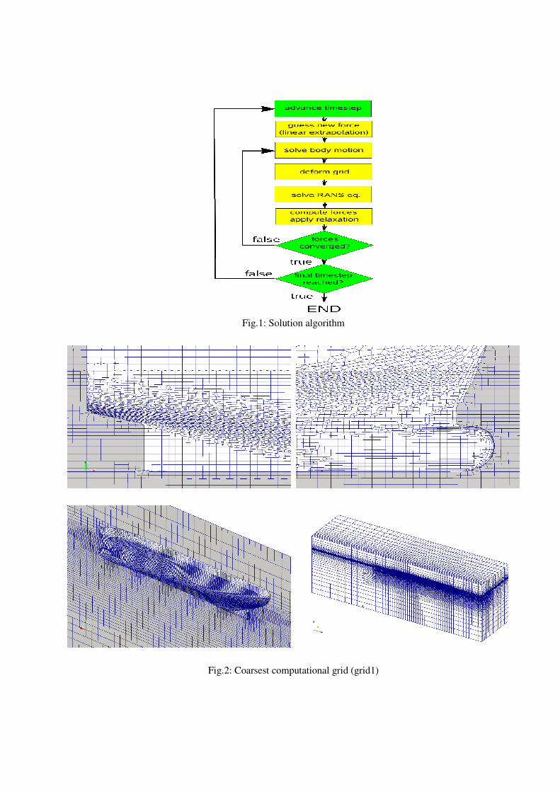
Fig.1: Solution algorithm

Fig.2: Coarsest computational grid (grid1)

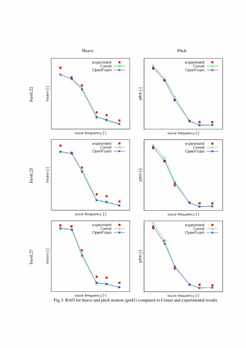
Heave Pitch

Fn

=0

.22

Fn=

0.2

5

Fn

=0

.27

Fig.3: RAO for heave and pitch motion (grid1) compared to Comet and experimental results

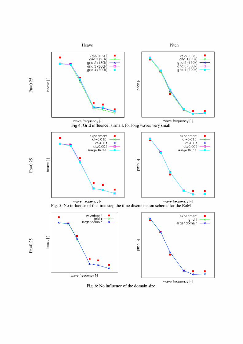
Heave Pitch

Fn

=0.2

5

Fig 4: Grid influence is small, for long waves very small

Fn

=0

.25

Fig. 5: No influence of the time step the time discretisation scheme for the EoM

Fn

=0

.25

Fig. 6: No influence of the domain size

Numerical Study of Cavitating Flows around a Flat Plate

Mohammad S. Seif, Abolfazl Asnaghi, Sharif University of Technology, Tehran/Iran

seif@sharif.edu, asnaghi_abolfazl@yahoo.com

The present study focuses on the simulation of two dimensional unsteady cavitating flows by using the

concept of phase change thermodynamic probability. For simulation of unsteady behaviors of

cavitation which have practical applications, the unsteady PISO algorithm based on the non-

conservative approach is utilized. To increase the stability of the PISO algorithm in solving cavitating

flows, some modifications are performed that will be presented in the full paper. For multi-phase

simulation, single-fluid Navier–Stokes equations, along with the volume fraction transport equation,

are employed.

To investigate the non-equilibrium effects of phase change in cavitating flows, the concept of phase

change thermodynamic probability is used along with homogeneous model to simulate two-phase

cavitating flows. In the full paper, whole details related to phase change thermodynamics probabilities

and cavitation model will be presented. Unsteady simulation of cavitation around a flat plate normal to

flow direction is performed to clarify accuracy of presented model. Based on the implied phase change

model, the cavitating flow behind the flat plate has been simulated in a good agreement with the

experimental results. To compare the presented model with other models, the numerical results are

also compared with Bubble Dynamics model and State Equation model results. Moreover, the

separation of the cavitation is clearly predicted by the developed CFD-code. These predictions provide

detailed information that will be helpful for understanding behaviors of unsteady cavity flows such as

cavitation inception and development. The effects of vapor generation on drag reduction are

investigated and will be presented. It is shown that by growth of cavity and reduction of cavitation

number, average drag coefficients reduce. Numerical results and comparisons with experimental data

will be provided. Some parts of obtained results are presented in this extended abstract paper.

1. Main parameters

When local static pressure of liquid falls below the corresponding saturated pressure, the phase of fluid

changes from liquid into vapor. This phenomenon is named cavitation. Cavitation is categorized by a

dimensionless number called the cavitation number, where it depends on saturated pressure, flow

reference pressure, density and velocity, respectively. The cavitation number is defined as follows:

(1) ∞∞

−=

U

PPsat

ρ

σ

2

1

In this study, the flow is assumed isothermal and fluid properties are supposed to be constant at a

given temperature for the entire flow domain. The saturated pressure, Pv, is set to a constant value of

2340 Pa.

2. Results

2.1 Geometry and Boundary Conditions

The computational domain and geometry for this study are presented in Fig.(1). The constant velocity

inlet and constant pressure outlet are considered as inlet and outlet boundaries. The main results are

obtained by considering outlet static pressure equal to 17965 Pa, and variations of velocity to adjust

cavitation numbers.

2.2 Unsteady behavior of cavitation

For considering unsteady behavior of fully cavitating flows behind the flat plate, the formation of

cavitation and its oscillations are presented as snapshots of unsteady behaviors for several cavitation

numbers in Fig.(2). The cavitation numbers are set equal to 1.0, 1.25 and 1.5. As presented in Fig.(2),

supercavitation is formed behind the flat plate in these conditions. At the end of these cavities, the two

phase vortex shedding occurs, and vapor is separated from the cavity by vortexes and moved to the

down stream.

2.3 Cavity Dimensions

One of the most important characters of cavitating flows is their cavity dimensions. The cavity

dimensions are usually normalized by a reference length which is the height of the flat plate, here. The

vapor iso-surfaces are presented in Fig.(3). Non-dimensional cavity length and width are presented in

Fig.(4) and Fig.(5).

2.4 Drag Forces

In the flow around of the flat plate, drag force is mainly pressure drag force. Therefore, by integrating

pressure distributions, average drag forces can be obtained. In the Fig.(6), variations of average drag

coefficient against cavitation number are presented. In this figure, experimental results by Waid [1],

the bubble dynamics model [2], the state equation model [3], and the free stream prediction [4] are

presented together with present numerical results. In the Fig.(6), it is presented that by development

of cavitation and reduction of cavitation numbers of the flow, the drag force coefficient reduces.

3. Conclusion

Unsteady behavior of cavitation around a flat plate oriented normal to flow direction is performed to

prove the accuracy of the utilized method in simulation of cavitating flows. To compare the presented

model with other models, the numerical results are also compared with Bubble Dynamics model and

State Equation model results. The shape and size of the vapor region and the separation of the

cavitation are clearly predicted by the developed CFD-code. These predictions provide detailed

information that will be helpful for understanding behaviors of unsteady cavity flows such as

cavitation inception and development. The effects of vapor generation on drag reduction are

investigated and presented. It is shown that by growth of cavity and reduction of cavitation number,

average drag coefficients reduce.

In the full paper, more details related to thermodynamics concepts, the modified PISO algorithm

related to cavitation simulations, details of governing equations, and analyzing of results will be

presented.

References

[1] Waid RL (1957) Water tunnel investigation of two-dimensional cavities. In: Knapp RT, Daily JW,

Hammitt FG (eds) Cavitation. McGraw-Hill Book Co, New York, pp. 188–194

[2] A. Asnaghi, E. Jahanbakhsh, M.S. Seif, “Drag Force on a Flat Plate in Cavitation Flows”,

Submitted, International Journal of Numerical Methods for Heat and Fluid Flow.

[3] Shin B.R., Iwata Y., Ikohagi T., 2003, ‘‘Numerical simulation of unsteady cavitating flows using a

homogenous equilibrium model,’’ J. Comput. Mechanics., 30, pp. 388-395.

[4] Knapp RT, Daily JW, Hammitt FG (1970) Cavitation. McGraw- Hill Book Co, New York, pp.

151–217

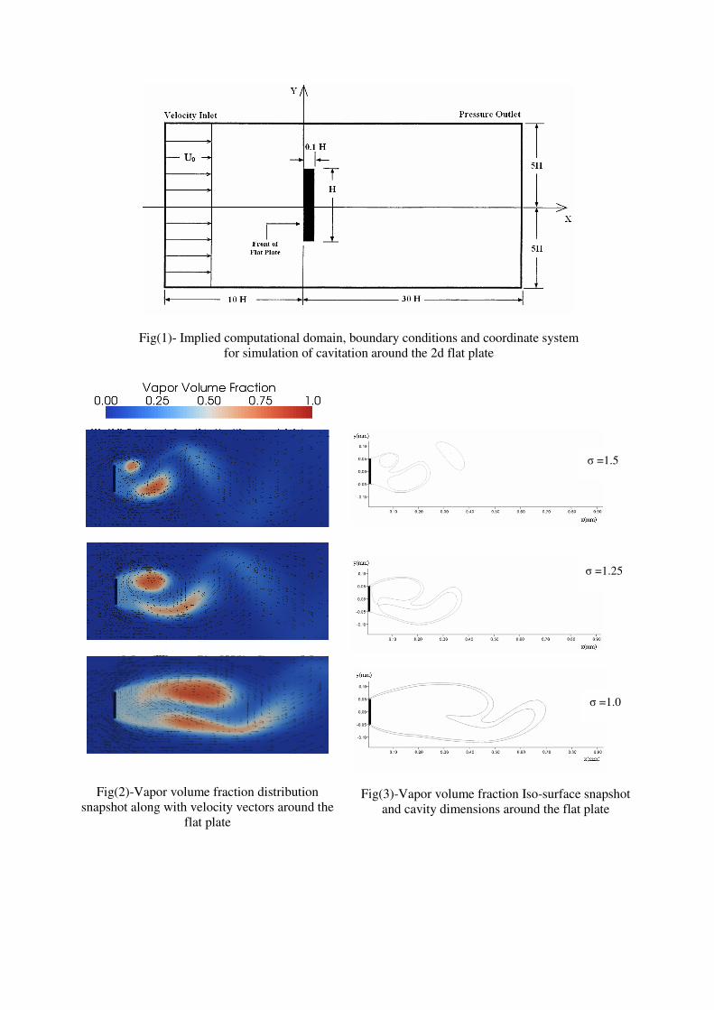
Fig(1)- Implied computational domain, boundary conditions and coordinate system

for simulation of cavitation around the 2d flat plate

Fig(2)-Vapor volume fraction distribution

snapshot along with velocity vectors around the

flat plate

Fig(3)-Vapor volume fraction Iso-surface snapshot

and cavity dimensions around the flat plate

σ =1.0

σ =1.25

σ =1.5

Fig(4)- Non-dimensional cavity width defined

by α=0.5

Experimental data by Waid [1], State Equation

Model [3] ,

Bubble Dynamics Model[2]

Fig(5)- Non-dimensional cavity length defined by

α=0.5

Experimental data by Waid [1], State Equation

Model[3] , Bubble Dynamics Model[2]

Fig(6)- Average drag coefficient of the 2d flat plate for several cavitation number

Experimental data by Waid [1], State Equation Model[3],

Free Stream Theory[4], Bubble Dynamics Model[2]

Analysis of numeri al models for avitation on 2D hydrofoilKeun Woo Shin (kwsmek.dtu.dk), Poul Andersen, Wen Zhong ShenDept. of Me hani al Engineering, Te hni al University of Denmark1 Introdu tionA avitation model is on the way to be implemented in the in ompressible Reynolds-averaged Navier-Stokes equation (RANSE) solver EllipSys3D in order to omplement model tests and existing numeri almethods for resear h on marine propellers. EllipSys3D is developed by the Department of Me hani alEngineering at the Te hni al University of Denmark and the Department of Wind Energy at Risø NationalLaboratory [6, 9. As a preliminary step, several avitation models are implemented in the 2D version ofEllipSys3D, and a omparative study between them and an analysis on the inuen e of some parametersare made.Numeri al models for avitation an be ategorized into two groups: single-phase interfa e tra kingmodel and multi-phase homogeneous equilibrium model. The former approa h, generally adopted forpotential ow methods, is less robust, requiring preliminary iterative pro edures. The se ond approa his suitable for RANSE solvers and an be applied to three-dimensional and unsteady ows, in ludingturbulen e u tuations and ompressibility ee ts. Mass transfers between the two phases are based oneither a vapor transport equation or a barotropi state law. Three avitation models using a transportequation and one model using a state law are implemented in EllipSys2D.2 Mathemati al formulationA single set of RANSE for the mixture ow with the mixture density ρ and the dynami vis osity µ issolved. The momentum equation is∂

∂t(ρui) +

∂

∂xj

(ρuiuj) −∂

∂xj

[

(µ + µt)

(∂ui

∂xj

+∂uj

∂xi

)]

+∂p

∂xi

= 0 (1)To avoid interpolating ρ on a ell fa e, we extra t ρ from the derivatives, whi h results inρ

(∂ui

∂t+

∂

∂xj

(uiuj)

)

+ ui

Dρ

Dt−

∂

∂xj

[

(µ + µt)

(∂ui

∂xj

+∂uj

∂xi

)]

+∂p

∂xi

= 0 (2)The ontinuity equation is written in the form of inhomogeneous divergen e equation as∂uj

∂xj

= −1

ρ

Dρ

Dt(3)Three avitation models using a transport equation are onsidered: Singhal's [4, 8, Zwart's [12 andKunz' [10. They are some of the most popular models, implemented in the ommer ial solvers FLUENT,ANSYS CFX and the opensour e solver OpenFOAM, respe tively.In Singhal's model [4, 8, a generi transport equation is solved for the vapor mass fra tion f as

∂

∂t(ρf) +

∂

∂xj

(ρujf) −∂

∂xj

(µt

Prv

∂f

∂xj

)

= −m (4)where Prv is the turbulent Prandtl number for vapor and m is the mass transfer rate per unit volume.m is related to the sour e term, based on the Rayleigh-Plesset equation as

m =

−Ce

√k

Tρlρv

√23

pv−pρl

(1 − f) for p < pv

Cc

√k

Tρ2

l

√23

p−pv

ρl

f for p > pv

(5)where Ce, Cc are empiri al oe ients for evaporation and ondensation, respe tively, k is the turbulen ekineti energy and T is the surfa e tension, T = 0.0717N/m. In evaporation for p < pv, the mass in the ontrol volume is de reased when transferring from liquid phase to vapor.In Zwart's model [12, the transport equation for the vapor volume fra tion αv is solved withoutdiusion term as∂

∂t(ρvαv) +

∂

∂xj

(ρvujαv) = −m (6)

wherem =

−Ce3rnucρv

RB

√23

pv−pρl

(1 − αv) for p < pv

Cc3ρv

RB

√23

p−pv

ρl

αv for p > pv.(7)and where RB is the bubble radius in the nu leation site, RB = 10−6 and rnuc is the nu leation sitevolume fra tion, rnuc = 5 · 10−4.In Kunz' model [10, the transport equation for the liquid volume fra tion αl is solved as

∂

∂t(ρlαl) +

∂

∂xj

(ρlujαl) = m (8)where m = m− + m+ andm− =

Ceρvαl min(0, p − pv)

0.5ρlU2∞t∞

, m+ =Ccρvα2

l (1 − αl)

t∞(9)and where U∞, t∞ are the referen e velo ity and the time s ale, respe tively, for whi h the inlet velo ityand C/U∞ are taken in the hydrofoil ase with the hord lenght C.The similarity of all three models omes from the relations

ρf = ρvαv =mv

Vt

, ρ(1 − f) = ρlαl =ml

Vt

, −ρlmv

Vt

=ρvml

Vt

=ρvρlm

ρ(10)where mv, ml, mv, ml are the vapor/liquid masses and the vapor/liquid mass transfer rates, respe tively,in the omputational ell and Vt is the total volume of the omputational ell.

−2 −1.5 −1 −0.5 0−7

−6

−5

−4

−3

−2

−1

0

1

CP + σ

m

0 0.5 1 1.5 2−0.05

0

0.05

0.1

0.15

0.2

0.25

0.3

0.35

0.4

0.45

CP + σ

SinghalZwartKunz

p

ρ

pv

ρv

ρla

min=0.5

amin

=1.0

Figure 1: The omparison of m from several avitation models (left, entre) and the barotropi state law(right)The values of m from the three models are given as a fun tion of CP + σ in Figure 1. In omputingm, the vapor fra tion is oupled with p through a barotropi state law in Eq.(15) for a rough omparison.The following values are applied to the oe ients for the omparison in Figure 1 and the omputationof the ow around a hydrofoilModel Singhal Zwart Kunz

Ce , Cc 0.08 , 0.02 0.5 , 5 · 10−5 2000 , 100The value of m from Singhal's model is omparatively large in evaporation, be ause the value of kis assumed to be 0.1, whi h is as large as that in highly turbulent regions at the leading edge and rightbehind the avity. While the saturation pressure is a bit lower than pv in Kunz' model, it is exa tly pvin the other ones. The pressure oe ient CP and the avitation number σ areCP =

p − p∞0.5ρlU2

∞, σ =

p∞ − pv

0.5ρlU2∞

(11)The mixture density and the dynami vis osity are omputed asρ = αvρv + (1 − αv)ρl , µ = αvµv + (1 − αv)µl (12)

By Eq.(12), the momentum and ontinuity equations are related to the sour e term of vapor transportequations asρ

(∂ui

∂t+

∂

∂xj

(uiuj)

)

+ ui

(1

ρl

−1

ρv

)

ρm −∂

∂xj

[

(µ + µt)

(∂ui

∂xj

+∂uj

∂xi

)]

+∂p

∂xi

= 0 (13)∂uj

∂xj

=

(1

ρl

−1

ρv

)

m (14)A avitation model using a barotropi state law [2 is also onsidered. The mixture density is dire tly oupled with the pressure through a state lawρ(p) =

ρl for p > pv + ∆pρv for p < pv − ∆p

ρv + ∆ρ[

1 + sin(

p−pv

∆ρa2

min

)] elsewhere (15)where amin is the minimum speed of sound in the liquid/vapor mixture and ∆ρ = ρl−ρv

2 , ∆p =πa2

min∆ρ

2 .The smaller amin is, the steeper the transition is, as shown in Fig 1 (right).For all omputations, the standard k − ω turbulen e model [11 is used.3 ImplementationThe dis retisation is based on the ollo ated nite volume method. The time derivative is approximatedby the se ond-order ba kward dierentiation s heme.Sin e ρ is outside the onve tive term in Eq.(13) and the divergen e term does not ontain ρ in Eq.(14),the volume ux on the ell fa e is al ulated using Rhie-Chow interpolation, instead of al ulating massux. The onve tive oe ients are estimated by upwind dieren ing s heme using volume ux andafterwards they are multiplied by ρ on the entre ell. ( 1ρl

−1ρv

)

ρm∆V is added to the entre- ell oe ient, where ∆V is the volume of omputational ell.The pressure- orre tion method is based on the SIMPLE s heme, but the sum of volume ux is thesour e term and the term with m is to be onsidered. Sin e m is dependent on the orre ted pressure p′as well, the total mass transfer rate m∗ taking a ount of p′ is approximated as [5m∗ =

∂m

∂p(p + p′ − pv) = p′

∂m

∂p+ m (16)where p is the pressure obtained from the momentum equation and m is found from the sour e term inthe vapor transport equation.The rst term with p′ is impli itly treated and the se ond term m is expli itly treated. It results inthe integral form of the pressure- orre tion equation as

(AP +

(1

ρl

−1

ρv

)

∆V∂m

∂p)p′P +

∑

nb

Anbp′nb =

∑

f

(uS)f −

(1

ρl

−1

ρv

)

∆V m (17)The derivative of m is∂m

∂p=

m

2(p−pv) in Singhal's and Zwart's modelsCeρvαl

0.5ρlU2∞

t∞for p < pv in Kunz' model (18)In the model with a state law, we use the derivative term of ρ in Eq.(3) and it is approximated as

1

ρ

Dρ

Dt=

[

(ρ − ρt−∆t)∂

∂p

(1

ρ

)

+1

ρ

(

∂ρ

∂p−

∂ρ

∂p

t−∆t)]

︸ ︷︷ ︸

γ

(p + p′ − pv) (19)where ρt−∆t, ∂ρ∂p

t−∆t is the density and the derivative of density, respe tively, at the previous time-stepand the derivatives are∂ρ

∂p= −

1

a2min

cos

(p − pv

∆ρa2min

)

,∂

∂p

(1

ρ

)

= −1

ρ2

∂ρ

∂p(20)A ordingly the pressure- orre tion equation be omes

(AP + γ∆V )p′P +∑

nb

Anbp′nb =

∑

f

(uS)f − γ∆V (p − pv) (21)

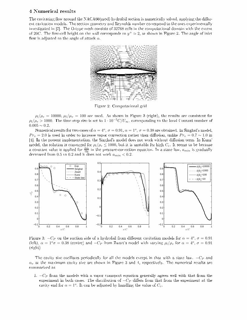
4 Numeri al resultsThe avitating ow around the NACA66(mod) hydrofoil se tion is numeri ally solved, applying the dier-ent avitation models. The se tion geometry and Reynolds number orrespond to the ones experimentallyinvestigated in [7. The O-type mesh onsists of 32768 ells in the omputational domain with the extentof 20C. The rst- ell height on the wall orresponds to y+ ≃ 2, as shown in Figure 2. The angle of inletow is adjusted to the angle of atta k α.

Figure 2: Computational gridρl/ρv = 10000, µl/µv = 100 are used. As shown in Figure 3 (right), the results are onsistent for

ρl/ρv > 1000. The time-step size is set to 1 · 10−5C/U∞, orresponding to the lo al Courant number of0.005 ∼ 0.2.Numeri al results for two ases of α = 4o, σ = 0.91, α = 1o, σ = 0.38 are obtained. In Singhal's model,Prv = 2.0 is used in order to in rease vapor onve tion rather than diusion, unlike Prv = 0.7 ∼ 1.0 in[4. In the present implementation, the Singhal's model does not work without diusion term. In Kunz'model, the solution is onverged for ρl/ρv ≤ 1000, but it is unstable for high Ce. It seems to be be ausea onstant value is applied for ∂m

∂pin the pressure- orre tion equation. In a state law, amin is graduallyde reased from 0.5 to 0.2 and it does not work amin < 0.2.

0 0.2 0.4 0.6 0.8 1−0.1

0

0.1

0.2

0.3

0.4

0.5

0.6

0.7

0.8

0.9

x/C

−C

p

ExpSinghalZwartKunzState law

0 0.2 0.4 0.6 0.8 1−0.2

−0.1

0

0.1

0.2

0.3

0.4

0.5

x/C0 0.2 0.4 0.6 0.8 1

−0.1

0

0.1

0.2

0.3

0.4

0.5

0.6

0.7

0.8

0.9

x/C

ρ

l/ρ

v=10000

ρl/ρ

v=1000

ρl/ρ

v=100

ρl/ρ

v=10

Figure 3: −CP on the su tion side of a hydrofoil from dierent avitation models for α = 4o, σ = 0.91(left), α = 1oσ = 0.38 ( entre) and −CP from Zwart's model with varying ρl/ρv for α = 4o, σ = 0.91(right)The avity size os illates periodi ally for all the models ex ept in that with a state law. −CP andαv at the maximum avity size are shown in Figure 3 and 4, respe tively. The numeri al results aresummarized as1. −CP from the models with a vapor transport equation generally agrees well with that from theexperiment in both ases. The distribution of −CP diers from that from the experiment at the avity end for α = 1o. It an be adjusted by handling the value of Cc.

Figure 4: αv from Singhal's, Zwart's, Kunz' models and the state law (from top to bottom) for α =4o, σ = 0.91 (left) and α = 1oσ = 0.38 (right)2. The avity size is a bit shorter than that from the experiment for α = 4o. The experiment mayhave a larger ee tive α due to the limited tunnel length and a dierent turbulen e hara teristi s.3. −CP behind the avity is larger than that from the experiment for α = 4o. It seems to be be ausethe loudy avitation is not realized. Dierent turbulen e models should be tried.4. For the model with a state law, the avity is not onve ted and hen e the avity remains at thelow-pressure region from the solution without the avitation model.5. The distribution of αv diers, as the distribution of m as a fun tion of p diers.

0 0.2 0.4 0.6 0.8 1−0.1

0

0.1

0.2

0.3

0.4

0.5

0.6

0.7

0.8

0.9

x/C

−C

p

C

e=0.1

Ce=0.3

Ce=0.7

0 0.2 0.4 0.6 0.8 1−0.1

0

0.1

0.2

0.3

0.4

0.5

0.6

0.7

0.8

0.9

x/C

Cc=3 ⋅ 10−5

Cc=5 ⋅ 10−5

Cc=7 ⋅ 10−5

Figure 5: −CP from Zwart's model with Cc = 5 · 10−5 (left) and with Ce = 0.5 (right)With Singhal's and Zwart's models, shown to be rather stable and a urate, we analyze the inuen eof Ce, Cc for the ase with α = 4o, σ = 0.91. The results are shown in Figure 5 and 6. There are ertainupper and lower limits on Ce, Cc for the numeri al solution to be stable. It is summarized as1. When Ce is smaller than a ertain value, it takes more time for the avity to be formed behind thelow pressure region at the leading edge and the avity size is rather small.2. When Ce is larger than a ertain value, the solution is onverged and no hange o urs.3. The smaller Cc is, the avity is ondensed more gradually with lower pressure gradient at the avityend.5 Con lusionSeveral avitation models are implemented in EllipSys2D and the numeri al results show that Singhal'sand Zwart's models are stable and a urate in our implementation. But the loudy avitation is not wellrealized. The avitation model is to be tested with dierent types of turbulen e models.

0 0.2 0.4 0.6 0.8 1−0.1

0

0.1

0.2

0.3

0.4

0.5

0.6

0.7

0.8

0.9

x/C

−C

p

C

e=0.06

Ce=0.08

Ce=0.10

0 0.2 0.4 0.6 0.8 1−0.1

0

0.1

0.2

0.3

0.4

0.5

0.6

0.7

0.8

0.9

x/C

C

c=0.01

Cc=0.02

Cc=0.03

Figure 6: −CP from Singhal's model with Cc = 0.02 (left) and with Ce = 0.08 (right)A way to improve the m derivative term in the pressure- orre tion equation for Kunz' model needs tobe devised for a hieving higher stability. The remedy for in luding vapor onve tion in the model with abarotropi state law needs to be found out.The oe ients Ce, Cc in evaporating and ondensing rates, respe tively, are shown to work a ordingto physi s and the avitation strength an be adjusted by alibrating them.A knowledgementThe advi es from the Institute of Fluid Dynami s and Ship Theory in Te hni al University of Hamburg-Harburg are gratefully a knowledged.Referen es[1 Frikha, S., Coutier-Delgosha, O., Astol, J. A. "Inuen e of the avitation model on the simulationof loud avitation on 2D foil se tion," Int. J. of Rotating Ma hinery, 2008[2 Hoeijmakers, H. W. M., Janssens, M. E., Kwan, W., "Numeri al simulation of sheet avitation," 3rdInt. Symp. on Cav., 1998[3 Kim, S. E., Brewton, S., "A multiphase approa h to turbulent avitating ows," 27th Symp. onNaval Hydrodyn., 2008[4 Rhee, S. H., Kawamura, T., Li, H. Y., "Propeller avitation study using an unstru tured grid basedNavier-Stokes Solver," ASME J. Fluids Eng.,2005[5 Maquil, T., "Simulation von instationaren kavitierenden Stromungen mit Hilfe von Mis hungs-bru hansatzen," Kleine Studienarbeit, TUHH, 2007[6 Mi helsen, J. A., Basis3D- A platform for development of multiblo k PDE solvers, Te hni al ReportAFM 92-05, DTU, Denmark, 1992[7 Shen, Y. J. and Dimotakis, J. S., "The inuen e of surfa e avitation on hydrodynami s for es,"22nd ATTC, 1989[8 Singhal, A. K., Athavale, M. M., Li, H. Y., Jiang, Y., "Mathemati al basis and validation of the full avitation model," ASME J. Fluids Eng., 2002[9 Sørensen N. N., General purpose ow solver applied to ow over hills, Risø, 2003[10 Wikstrom, N., "Modeling of avitating ow around a stationary/moving wing prole," 43rd AIAAAerospa e S . Meeting, Reno, NV, 2005[11 Wil ox, D. C. Turbulen e modeling for CFD, DCW Industries, In ., La Canada, CA, 2nd ed., 1994[12 Zwart, P. J., Gerber, A. G., Belamri T., "A two-phase ow model for predi ting avitation dynami s,"ICMF, 2004

Adjoint RANS for Hull Form Optimisation

Arthur Stuck, arthur.stueck@tu-harburg.deThomas Rung, thomas.rung@tu-harburg.de

Hamburg University of Technology (TUHH)Institute for Fluid Dynamics and Ship Theory (M-8)

Introduction

The use of sophisticated CFD techniques in aerospace, automotive or maritime industry hasoften been motivated through questions related to shape design and optimisation. Designengineers need to understand the dependency of the fluid dynamic design criteria on the keyflow features which, in turn, depend on the shape design. The chain can be described as:

Shape Parametrisation bi (i = 1, nb) → Flow → Objectives Jk (k = 1, nJ),

where bi are the design parameters influencing the objective function(s) Jk through the flow.When we are interested in shape modifications a corresponding chain describes the variationof parametrisation, flow and objectives. Following this intuitive direction is referred to asforward or direct sensitivity analysis. The simplest representative is finite differencing, out-lined as follows: Modify the shape, b′i = bi + εi, evaluate the perturbed flow and calculate thecost function derivative by δJ/δbi ≈ (J ′ − J)/εi. This requires at least nb + 1 cost functionevaluations for a first order approximation of the cost function derivative. Alternative directstrategies are Complex Variable techniques (avoiding numerical cancellations) or direct differ-entiation of the flow solver. Generally, the computational costs for direct sensitivity analysisare comparable to O(nb) cost function evaluations, i.e. the effort scales with the number ofparameters. Alternatively, in adjoint-based sensitivity analysis (Jameson, 1995), the com-putational effort scales with the number of cost functions, independently of the number ofparameters. This is achieved by eliminating the parameter-specific flow variations appearingin the direct approach via solving the cost function-specific adjoint problem.

Using viscous CFD, computational costs quickly become prohibitive. When many designparameters are involved, it is mostly impossible to vary all of them systematically in a directway. Often the design analysis is restricted of necessity to a parameter preset. This demon-strates the need for efficient shape analysis tools for viscous flow, such as the adjoint method.Flow sensitivities can be used to support both manual (Soding, 2001) and automaticshapedesign. The former is often preferred in industrial ship design as the formulation of designconstraints (operational, economic or manufacturability limitations) can be a very cumber-some task. Gradient-based optimisers, which are the workhorse of classic optimisation, alsorequire sensitivity information. If applicable (smooth/noisy cost functions), gradient-basedoptimisation can be very efficient compared against gradient-free approaches.

Einstein’s notation applies to the small-type latin subindices. When symbolic notation isused the number of underlines corresponds to the order of the tensor.

Primal RANS and Cost Functions

Design configurations, described via the shape parametrisation bi, are usually evaluated interms of some integral hydrodynamic cost functions or objectives, which may consist of

boundary- and/or volume-declared contributions:

J = JΓ + JΩ =∫

Γobj

jΓ dΓ +∫

Ωobj

jΩ dΩ . (1)

The flow domain is represented by Ω and its boundary is denoted by Γ. The integration iscarried out over Γobj∩Γ and Ωobj∩Ω, representing the objective volume(s) or surface(s).The flow is governed by the incompressible steady-state RANS equations

Ri = ρDUi

Dt− ∂πij

∂xj− fi = 0 and Q =

∂Ui

∂xi= 0 in Ω , (2)

where Ui, p and fi denote the mean velocity components, the modified mean pressure andbody force components. The stress tensor is defined as

πij = −p δij + 2µeffSij and Sij =12

(∂Ui

∂xj+

∂Uj

∂xi

). (3)

In accordance with the turbulence model applied, the eddy viscosity µT is obtained from theturbulence variables. The molecular viscosity µ is augmented by the eddy viscosity to givethe effective viscosity, i.e. µeff = µ + µT .

Variational Calculus

When the design surface Γdsg ⊂ Γ is subject to a small shape variation δbi (i = 1, nb), theinterior domain Ω has to follow the perturbation to avoid gaps in the perturbed domain. Therest of the boundaries, Γ \ Γdsg, remains unchanged. The spatial displacements correspondingto a change in the shape variables bi are

δxk =nb∑

i=1

(δbi

∂xk

∂bi

)on/in Γdsg , Ω . (4)

Note that the shift vector δxk corresponds to a particular realisation (or combination) ofshape parameter variations. Imposing the spatial perturbations (4) on the “old” (or original,subindex 0) domain yields the “new” (or modified, subindex 1) position

x1 = x0 + δx on/in Γdsg , Ω . (5)

A modification of the domain induces a change of the flow. With φ(0), φ(1) referring to theold and new flow respectively, the new flow at the new position can be written as

φ(1)∣∣x1

= φ(0)∣∣x0

+nb∑

i=1

δbi

[∂φ

∂bi+

∂xk

∂bi

∂φ

∂xk

]

x0

=[φ(0) + δlφ + δcφ

]x0

, (6)

with the local and convective flow variations δlφ and δcφ. This decomposition accounts forthe flow change at the old grid position (local variation) and the spatial variation of the oldflow due to a nodal position shift δxi (convective variation), respectively. The latter can beobtained from a truncated Taylor series expansion of the old flow about the old grid positionx0 :

δcφ∣∣x0≈ δxj

∂φ

∂xj

∣∣∣x0

. (7)

The subsequent analysis is carried out on the original grid, thus the indicators x0 are left outfor brevity. φ refers to the old flow unless declared explicitly. When the variational calculusis applied to the flow equations (2), we obtain:

δlRi = 0 and δlQ = 0 in Ω . (8)

Satisfying the primal RANS equations (2) implies that also the respective gradients of theresiduals vanish identically and Eqs. (8) contain local variations alone. Eqs. (8) governthe local flow variation corresponding to a particular shape perturbation. The boundaryconditions for the flow variation are presented in the following section; local and convectiveflow variations are coupled via the boundary conditions on the deformable boundaries Γdsg.Note that Eqs. (8) have to be evaluated on the original (non-deformed) domain Ω. Forincompressible flow the density shows no variation. A possible variation of the eddy-viscositywith respect to the shape is not taken into consideration, neither in terms of a convectivenor a local variation. This frozen-turbulence assumption is common practice (Othmer, 2007;Soto and Lohner, 2004).

As the shape variation originates from Γdsg, the boundary conditions on Γdsg are subjectto both convective and local variations. The boundary condition for the variation isobtained by postulating that the original boundary condition also holds for the modifiedboundary. A Dirichlet boundary condition postulated for the old flow φ(0) on the originaldomain boundary Γ0 also needs to be satisfied by the perturbed flow φ(1) on the modifiedgeometry Γ1, viz.

D = φ(0)∣∣Γ0

= φ(1)∣∣Γ1

=[φ(0) + δlφ + δcφ

]Γ0

à δlφ = −δcφ = −δxi∂φ

∂xion Γdsg . (9)

Variations of Neumann- and Robin-type boundary conditions can be derived accordingly.

Adjoint RANS Problem

The optimisation problem subject to the RANS equations can be turned into an uncon-strained problem via the Lagrangian calculus. The cost function is extended by the RANSconstraints weighted by the so-called Lagrange multipliers or adjoint variables (Ui, p):

L = J +∫

dΩ[Ui Ri − p Q

]. (10)

The adjoint variables are field variables, as their corresponding primal counterparts. Giventhat the RANS equations are satisfied for the reference case (design state investigated), thisexpression meets exactly the cost function value J . The cost function gradient is obtainedfrom the variation of the extended cost function

δL = δlcJ + δgJ +∫

ΩdΩ

[Ui δlRi − p δlQ

]+

∫

δΩdΩ

[Ui Ri − p Q

]. (11)

The variation of the domain (last right-hand side integral above) is zero if the referenceflow equations are satisfied. When the variation of the RANS constraints (or cost functionextension) is satisfied, the variation of the Lagrangian matches the variation of the costfunction, i.e. δL = δJ . The basic idea is to chose the adjoint multipliers (Ui, p) such thatany contribution to Eq. (11) depending on local flow variations is eliminated. This particularchoice (Ui, p) requires to satisfy the adjoint RANS equations, which are cost function specific.After solving the adjoint problem once per cost function, the cost function derivatives arecheaply obtained for an arbitrary number of shape parameters by evaluating the remainingterms.

Integration by parts of Eq. (11) yields the adjoint field equations and boundary conditions,which eliminate the local flow variations for arbitrary/admissible choices (δlUi, δlp). Theadjoint field equations are

−2ρUjSij =∂

∂xj

(2µeff Sij − p δij

)− ∂jΩ

∂Uiin Ωobj

−2ρUjSij =∂

∂xj

(2µeff Sij − p δij

)in Ω \ Ωobj

(12)

and

∂Ui

∂xi=

∂jΩ

∂pin Ωobj

∂Ui

∂xi= 0 in Ω \ Ωobj ,

(13)

where the cost function integrand has been expressed as

δljΩ = δlp∂jΩ

∂p+ δlUi

∂jΩ

∂Ui. (14)

The corresponding adjoint boundary conditions are presented in Table 1.

Table 1: Summary of boundary conditions for the adjoint RANS equations. d specifies thedirection of the force component used as cost function.

boundary Ut Un p objective

no-slip wall on Γ \ Γobj Ut = 0 Un = 0 p,n = 0 -no-slip wall on Γobj Ut = −di ti Un = −di ni p,n = 0 forceslip wall Ut,n = 0 Un = 0 p,n = 0 -inflow Ut = 0 Un = 0 p,n = 0 -pressure outflow ρUnUt + µeff Ut,n = 0 p = ρUnUn + ρUjUj + µeff Un,n -farfield outflow Ut = 0 Un = 0 p,n = 0 -

Having augmented the cost function by the RANS-constraints first, and having eliminatedthe local flow variations through satisfying the adjoint RANS equations second, the remainingterms of Eq. (11) make the adjoint sensitivity equation. After some transformation theadjoint sensitivity equation for boundary-normal shape perturbations, δn = δx · n, becomes:

δJ =∫

δΓobj

jΓ dΓ−∫

Γdsg

dΓ

[µeff δn

∂Ut

∂n

∂Ut

∂n

]. (15)

The leading right-hand side term denotes the partial variation with respect to the surfacegeometry. It can cheaply be evaluated based on the old flow at the old surface location byintegration over the surface variation. According to the chain rule it can be decomposed intoa change of the surface orientation and the surface area; for a generic boundary-defined costfunction jΓ = φ · n, we obtain

∫

δΓobj

jΓ dΓ =∫

δΓobj

φ · n dΓ ≈∑

cellFaces

[φ · (δn ∆Γ + n δ [∆Γ])

]on Γobj . (16)

Note that the second right-hand side integral of Eq. (15) is restricted to the design surface.

Primal and Adjoint RANS Solvers

The incompressible RANS equations are solved using a collocated cell-centred finite volumediscretisation on unstructured grids. Pressure-velocity coupling is enforced via SIMPLE-likepressure correction schemes. The same approach is used for the adjoint code, i.e. Eqs. (12)and (13) are solved using an adapted SIMPLE scheme.The adjoint code is written closest possible to the primal RANS solver. Coding effort cansignificantly be reduced by reusing huge portions of the original solver (approx. 90 per

cent). Consistency of both primal and adjoint discretisation (duality) minimises potentialmismatches between the cost function values calculated by the primal solver and its variationsobtained with the adjoint code (Nadarajah, 2003).

The adjoint technique traces the sensitivity back from the objective volume(s) or sur-face(s), Γobj or Ωobj, to the design surface(s) Γdsg. In other words, the information is back-tracked from the receiver to the sender. This reverse or backwards strategy is reflected, forexample, in the negative convection direction of the adjoint equations. In discrete adjointtechniques based on automatic differentiation, the adjoint code runs in opposite directionfrom the cost function evaluation to the influence parameters at the beginning of the forwardcode.

Examples

A NACA0012 wing section at Re = 105 was investigated first, using a structured mesh ofapprox. 16 kCells. The base-line k-ω turbulence model was applied resolving the viscousshear layer numerically (LowRE) with y+ values O(1). Lift and drag forces acting on the foilsurface Γobj were selected as cost function:

JΓ =∫

Γobj

jΓ dΓ with jΓ = −πij di nj , (17)

with the boundary normal n and d = e1 or d = e2 for cost function drag and lift, respectively.

Figure 1: Shape sensitivities for a NACA0012 at Re = 105, 5 angle of attack. The shape-normal sensitivities are shown for the lift-objective (left) and a weighted lift-drag objective(glide angle, right). The left picture also shows the adjoint velocity and pressure distributionfor the lift-objective.

A KVLCC2 ship hull was investigated next. The first tests were carried out at Re = 5·105,with a no-slip boundary condition at the still water surface. The base-line k-ω turbulencemodel and LowRe wall boundary conditions on the ship hull were applied. The underlyingmesh had 350 kCells and was generated with the HEXPRESS mesh generator. The viscousdrag of the hull was investigated (d = e1). Moreover a homogeneity criterion in the propellerdisk was considered as cost function:

JΩ =∫

Ωobj

jΩ dΩ with jΩ =12

(Ui − U trg

i

)2, (18)

where Ωobj denotes the propeller disk volume and U trgi is the desired target velocity profile.

Figure 2: Drag sensitivities for a KVLCC2 hull at Re = 5 · 105. Left: Following the arrowsreduces the viscous drag. Right: The (negative) shape-normal sensitivities have been imposedon the original hull (blue) through a morphing feature (red).

Conclusions and Outlook

The 3-D unstructured finite volume RANS solver FreSCo+ has been extended by an adjointsolver in order to aid in the shape design of ship hulls. This is a very cost-effective wayto obtain the sensitivities of an objective function with respect to surface design modifica-tions. The method yields considerable insight from the objective point of view, providing acontinuous sensitivity distribution over the design surface (ship hull, rudder, airfoils etc.).

A number of improvements will be required to prepare the adjoint technique for productionuse; among them:

• Provide the data interfaces to existing CAD/CAE frameworks.

• Extend the adjoint formulation to further cost functions.

• Optimise the adjoint solver (stability, numerical treatment of new terms).

• Improved turbulence treatment.

References

A. Jameson. Optimum aerodynamic design using CFD and control theory. 12th AIAAComputational Fluid Dynamics Conference (95-1729), June 1995.

S. K. Nadarajah. The Discrete Adjoint Approach to Aerodynamic Shape Optimization. PhDthesis, Stanford University, Jan. 2003.

C. Othmer. A continuous adjoint formulation for the computation of topological and surfacesensitivities of ducted flows. Int. J. Numer. Meth. Fluids, page 125, 2007.

O. Pironneau. Optimal shape design for elliptic systems. Springer Series in ComputationalPhysics. Springer-Verlag, 1984.

H. Soding. Hull shape design for reduced resistance. Ship Research Technology, 48:135–144,2001.

O. Soto and R. Lohner. On the computation of flow sensitivities from boundary inte-grals. 42th AIAA Aerospace Sciences Meeting and Exhibit, Reno, Nevada, 2004. URLhttp://www.scs.gmu.edu/~rlohner/pages/publications/design.html.

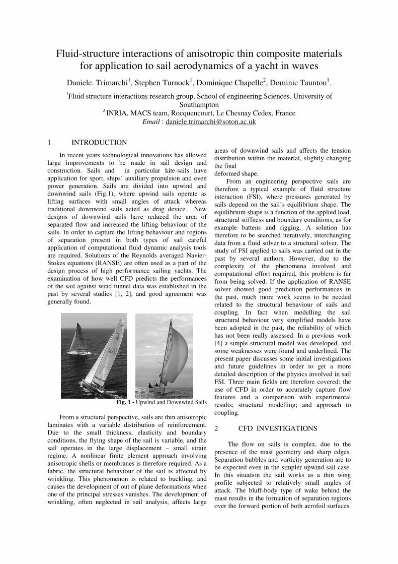
Fluid-structure interactions of anisotropic thin composite materials

for application to sail aerodynamics of a yacht in waves

Daniele. Trimarchi1, Stephen Turnock

1, Dominique Chapelle

2, Dominic Taunton

1.

1Fluid structure interactions research group, School of engineering Sciences, University of

Southampton 2 INRIA, MACS team, Rocquencourt, Le Chesnay Cedex, France

Email : daniele.trimarchi@soton.ac.uk

1 INTRODUCTION

In recent years technological innovations has allowed

large improvements to be made in sail design and

construction. Sails and in particular kite-sails have

application for sport, ships’ auxiliary propulsion and even

power generation. Sails are divided into upwind and

downwind sails (Fig.1), where upwind sails operate as

lifting surfaces with small angles of attack whereas

traditional downwind sails acted as drag device. New

designs of downwind sails have reduced the area of

separated flow and increased the lifting behaviour of the

sails. In order to capture the lifting behaviour and regions

of separation present in both types of sail careful

application of computational fluid dynamic analysis tools

are required. Solutions of the Reynolds averaged Navier-

Stokes equations (RANSE) are often used as a part of the

design process of high performance sailing yachts. The

examination of how well CFD predicts the performances

of the sail against wind tunnel data was established in the

past by several studies [1, 2], and good agreement was

generally found.

Fig. 1 - Upwind and Downwind Sails

From a structural perspective, sails are thin anisotropic

laminates with a variable distribution of reinforcement.

Due to the small thickness, elasticity and boundary

conditions, the flying shape of the sail is variable, and the

sail operates in the large displacement – small strain

regime. A nonlinear finite element approach involving

anisotropic shells or membranes is therefore required. As a

fabric, the structural behaviour of the sail is affected by

wrinkling. This phenomenon is related to buckling, and

causes the development of out of plane deformations when

one of the principal stresses vanishes. The development of

wrinkling, often neglected in sail analysis, affects large

areas of downwind sails and affects the tension

distribution within the material, slightly changing

the final

deformed shape.

From an engineering perspective sails are

therefore a typical example of fluid structure

interaction (FSI), where pressures generated by

sails depend on the sail’s equilibrium shape. The

equilibrium shape is a function of the applied load,

structural stiffness and boundary conditions, as for

example battens and rigging. A solution has

therefore to be searched iteratively, interchanging

data from a fluid solver to a structural solver. The

study of FSI applied to sails was carried out in the

past by several authors. However, due to the

complexity of the phenomena involved and

computational effort required, this problem is far

from being solved. If the application of RANSE

solver showed good prediction performances in

the past, much more work seems to be needed

related to the structural behaviour of sails and

coupling. In fact when modelling the sail

structural behaviour very simplified models have

been adopted in the past, the reliability of which

has not been really assessed. In a previous work

[4] a simple structural model was developed, and

some weaknesses were found and underlined. The

present paper discusses some initial investigations

and future guidelines in order to get a more

detailed description of the physics involved in sail

FSI. Three main fields are therefore covered: the

use of CFD in order to accurately capture flow

features and a comparison with experimental

results; structural modelling; and approach to

coupling.

2 CFD INVESTIGATIONS

The flow on sails is complex, due to the

presence of the mast geometry and sharp edges.

Separation bubbles and vorticity generation are to

be expected even in the simpler upwind sail case.

In this situation the sail works as a thin wing

profile subjected to relatively small angles of

attack. The bluff-body type of wake behind the

mast results in the formation of separation regions

over the forward portion of both aerofoil surfaces.

In addition, trailing edge separation is expected, due to the

adverse pressure gradient towards the rear of the aerofoil

upper surface. An important reference in this analysis is

given by Wilkinson’s [5, 6]. In these experiments, carried

out in Southampton in the early 80’s, a lower third section

of a typical yacht mainsail with a mast was tested in the

wind tunnel. Measurements were carried out in terms of

velocity profiles, pressures and separation bubble lengths.

In the case analysed later the ratio of mast diameter to sail

chord was 4.03% with a camber to chord ratio of 12.5%.

The angle of incidence of the sail was 5 degrees at a

Reynolds’ number of 709000. The camber distribution

represents that of a NACA a=0.8 mean line. The sail was

constructed from a 5 mm thick rigid aerofoil of 2.11m span

and 0.7m chord, fitted horizontally across the wind tunnel.

Pressure measurements were performed with pressure

tapings at mid span. Results from these experiments

suggest that a mainsail can be ideally divided into 9

regions, where different flow features can be identified, as

in Fig.2:

Fig. 2. Wilkinson's flow regions

Separations bubbles are widely developed on the sail

surface, and they are induced by the presence of the mast

both on leeward and windward side, and at the trailing

edge leeward side. In Fig.2 a universal pressure

distribution is represented, where it is possible to

appreciate that the influence of such bubbles in terms of

pressure coefficient is quite important and it cannot be

neglected. Results in terms of boundary layer velocity

profiles are given at specified locations as in Fig.3.

Fig. 3 - Wilkinson's measurements locations

These experiments are a good starting point as a

validation exercise, and they have been used in the past by

several authors [7, 8]. In particular, Paton’s analysis was

performed with the commercial RANSE solver ANSYS

CFX, the package which has been used also for the present

analysis.

In the past potential codes were also used for this kind

of analysis [9, 10]. Although this could be an effective way

to get easy and fast results, the inability to capture

separation bubbles is an important an unacceptable source

of error, as shown in Fig.2-b.

An initial multiblock structured - hexaedral

mesh with O-Grid around the mast has been

chosen, as in Fig.4. With such a mesh it is

generally possible to expect central symmetry at

all mesh points, this preserves second order

accuracy. However, in the future investigations

will be also carried out on hybrid meshes. With

hybrid meshes the computational effort in the

outer domain is slightly reduced, with a degree of

accuracy which can be on a par with structured

meshes [11]. However, in the literature structured

meshes have been chosen for sail analysis [1, 4].

A mesh independency analysis is reported for 4

different meshes, the characteristics of which are

reported in terms of spacing and average y+ over

the whole mast-sail geometry:

Table 1. Analyzed meshes. Mesh Total n.

elem.

Vertical

on mast

Vertical on

sail

Horizontal

on mast

AVG

y+

1 140.532 0.4 0.2 0.7 9

2 149.838 0.4 0.1 0.7 6.4

3 151.611 0.4 0.1 0.5 8.4

4 178.725 0.2 0.05 0.5 3.9

Fig. 4 – Mesh in the mast region

Generally sail flows are modelled as fully

turbulent, with a typical inlet free stream

turbulence of 5%. However, Wilkinson’s

experiments suggest that the mast flow is always

below transition, meaning that the boundary layer

on the mast is laminar. Transition is estimated

within the last 25% of separation bubble length, as

in Fig. 5. On the other hand, Collie [12] suggests

that for real sail flows transition to turbulence

could be accelerated by surface roughness and

fittings at the head of the sail.

Fig. 5 – Wilkinson’s observed transition

For the simulation SST turbulence model with

automatic wall treatment was chosen, since it is

considered as the most suitable for both upwind

and downwind sails [12]. This is generally accepted in sail

analysis literature, and just a few authors chose different

turbulence models. Simulations were carried out for fully

turbulent cases and for cases with transition. Unfortunately

convergence becomes very difficult in the case with

transition, and residuals remain about values of 410−

both

for steady or unsteady cases. For this reason results

presented here relates to the fully-turbulent case, and

further investigations will be carried on in the early future.

Velocity profile comparisons are presented in Fig.6,

where results from Wilkinson’s experiments,

Paton’s analysis and the current analysis (mesh 4)

are compared. As expected, the error decreases

with the distance from the separation bubble. A

remarkable mesh-sensitivity was experienced, and

the four meshes analyzed seem to be in the range

of convergence for this case. Further increasing or

decreasing spacing caused

severe convergence issues.

Fig. 6 – Velocity profiles comparison – results for Mesh 4

A comparison of Cp values is reported in Fig.7. The

general behaviour is captured, but errors are quite

important in correspondence to separation regions. In

Fig.8 a comparison between the present and Paton’s

analysis was performed in terms of relative error:

)( calculatedWilkinson

calculatedWilkinson

CpCpMIN

CpCpERROR

−

−= (1)

Error values from present and Paton’s analysis seem to be

comparable over the whole sail chord, except in the

leeward separation bubble region. Here Paton over

estimates the pressure value, where the current analysis

under estimates it.

Fig. 7 - Cp values comparison

Fig. 8 – Errors. Comparison with Paton’s Analysis

Fig. 9 – Mesh sensitivity over calculated forces

In Fig.9 values for Forces are plotted over a mesh

density parameter, obtained by multiplying the

spacing in Table1.Calculated forces are relatively

stable. On the other hand, in Fig.10, Cp plots are

reported on the same scale as Fig7 for the four

analyzed meshes. In this case it is remarkable the

difference between the treatment of the separation

bubble pressure, which is always poorly estimated,

but the finer mesh seems to better capture the flow

features experienced by Wilkinson. The relative

stability of measured forces in Fig.9 can therefore

be explained looking at Fig.10, observing that the

integral of all calculated Cp curves have similar

values.

Fig. 10 – Mesh sensitivity over calculated Cp

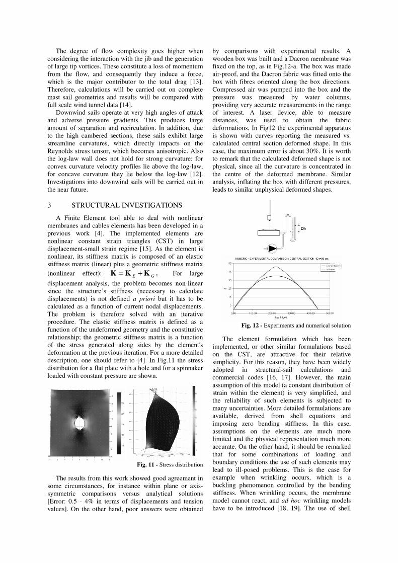
The degree of flow complexity goes higher when

considering the interaction with the jib and the generation

of large tip vortices. These constitute a loss of momentum

from the flow, and consequently they induce a force,

which is the major contributor to the total drag [13].

Therefore, calculations will be carried out on complete

mast sail geometries and results will be compared with

full scale wind tunnel data [14].

Downwind sails operate at very high angles of attack

and adverse pressure gradients. This produces large

amount of separation and recirculation. In addition, due

to the high cambered sections, these sails exhibit large

streamline curvatures, which directly impacts on the

Reynolds stress tensor, which becomes anisotropic. Also

the log-law wall does not hold for strong curvature: for

convex curvature velocity profiles lie above the log-law,

for concave curvature they lie below the log-law [12].

Investigations into downwind sails will be carried out in

the near future.

3 STRUCTURAL INVESTIGATIONS

A Finite Element tool able to deal with nonlinear

membranes and cables elements has been developed in a

previous work [4]. The implemented elements are

nonlinear constant strain triangles (CST) in large

displacement-small strain regime [15]. As the element is

nonlinear, its stiffness matrix is composed of an elastic

stiffness matrix (linear) plus a geometric stiffness matrix

(nonlinear effect): GE KKK += . For large

displacement analysis, the problem becomes non-linear

since the structure’s stiffness (necessary to calculate

displacements) is not defined a priori but it has to be

calculated as a function of current nodal displacements.

The problem is therefore solved with an iterative

procedure. The elastic stiffness matrix is defined as a

function of the undeformed geometry and the constitutive

relationship; the geometric stiffness matrix is a function

of the stress generated along sides by the element's

deformation at the previous iteration. For a more detailed

description, one should refer to [4]. In Fig.11 the stress

distribution for a flat plate with a hole and for a spinnaker

loaded with constant pressure are shown.

Fig. 11 - Stress distribution

The results from this work showed good agreement in

some circumstances, for instance within plane or axis-

symmetric comparisons versus analytical solutions

[Error: 0.5 - 4% in terms of displacements and tension

values]. On the other hand, poor answers were obtained

by comparisons with experimental results. A

wooden box was built and a Dacron membrane was

fixed on the top, as in Fig.12-a. The box was made

air-proof, and the Dacron fabric was fitted onto the

box with fibres oriented along the box directions.

Compressed air was pumped into the box and the

pressure was measured by water columns,

providing very accurate measurements in the range

of interest. A laser device, able to measure

distances, was used to obtain the fabric

deformations. In Fig12 the experimental apparatus

is shown with curves reporting the measured vs.

calculated central section deformed shape. In this

case, the maximum error is about 30%. It is worth

to remark that the calculated deformed shape is not

physical, since all the curvature is concentrated in

the centre of the deformed membrane. Similar

analysis, inflating the box with different pressures,

leads to similar unphysical deformed shapes.

Fig. 12 - Experiments and numerical solution

The element formulation which has been

implemented, or other similar formulations based

on the CST, are attractive for their relative

simplicity. For this reason, they have been widely

adopted in structural-sail calculations and

commercial codes [16, 17]. However, the main

assumption of this model (a constant distribution of

strain within the element) is very simplified, and

the reliability of such elements is subjected to

many uncertainties. More detailed formulations are

available, derived from shell equations and

imposing zero bending stiffness. In this case,

assumptions on the elements are much more

limited and the physical representation much more

accurate. On the other hand, it should be remarked

that for some combinations of loading and

boundary conditions the use of such elements may

lead to ill-posed problems. This is the case for

example when wrinkling occurs, which is a

buckling phenomenon controlled by the bending

stiffness. When wrinkling occurs, the membrane

model cannot react, and ad hoc wrinkling models

have to be introduced [18, 19]. The use of shell

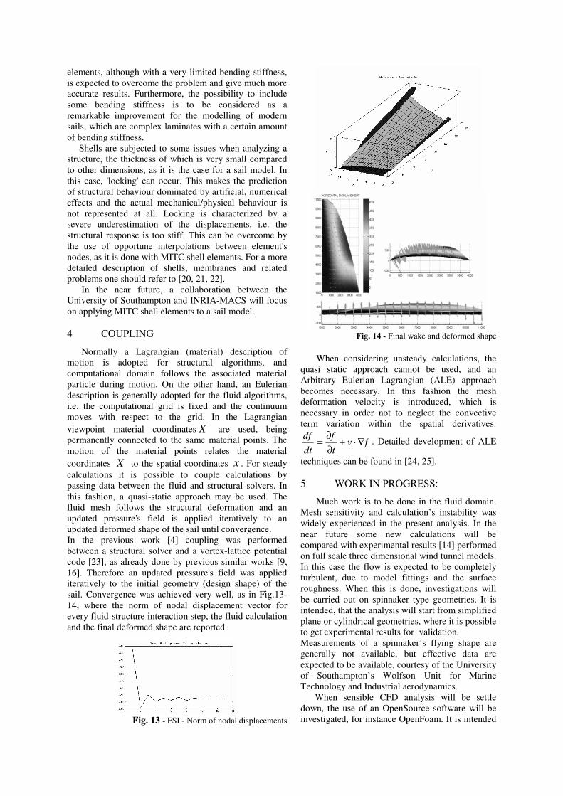
elements, although with a very limited bending stiffness,

is expected to overcome the problem and give much more

accurate results. Furthermore, the possibility to include

some bending stiffness is to be considered as a

remarkable improvement for the modelling of modern

sails, which are complex laminates with a certain amount

of bending stiffness.

Shells are subjected to some issues when analyzing a

structure, the thickness of which is very small compared

to other dimensions, as it is the case for a sail model. In

this case, 'locking' can occur. This makes the prediction

of structural behaviour dominated by artificial, numerical

effects and the actual mechanical/physical behaviour is

not represented at all. Locking is characterized by a

severe underestimation of the displacements, i.e. the

structural response is too stiff. This can be overcome by

the use of opportune interpolations between element's

nodes, as it is done with MITC shell elements. For a more

detailed description of shells, membranes and related

problems one should refer to [20, 21, 22].

In the near future, a collaboration between the

University of Southampton and INRIA-MACS will focus

on applying MITC shell elements to a sail model.

4 COUPLING

Normally a Lagrangian (material) description of

motion is adopted for structural algorithms, and

computational domain follows the associated material

particle during motion. On the other hand, an Eulerian

description is generally adopted for the fluid algorithms,

i.e. the computational grid is fixed and the continuum

moves with respect to the grid. In the Lagrangian

viewpoint material coordinates X are used, being

permanently connected to the same material points. The

motion of the material points relates the material

coordinates X to the spatial coordinates x . For steady

calculations it is possible to couple calculations by

passing data between the fluid and structural solvers. In

this fashion, a quasi-static approach may be used. The

fluid mesh follows the structural deformation and an

updated pressure's field is applied iteratively to an

updated deformed shape of the sail until convergence.

In the previous work [4] coupling was performed

between a structural solver and a vortex-lattice potential

code [23], as already done by previous similar works [9,

16]. Therefore an updated pressure's field was applied

iteratively to the initial geometry (design shape) of the

sail. Convergence was achieved very well, as in Fig.13-

14, where the norm of nodal displacement vector for

every fluid-structure interaction step, the fluid calculation

and the final deformed shape are reported.

Fig. 13 - FSI - Norm of nodal displacements

Fig. 14 - Final wake and deformed shape

When considering unsteady calculations, the

quasi static approach cannot be used, and an

Arbitrary Eulerian Lagrangian (ALE) approach

becomes necessary. In this fashion the mesh

deformation velocity is introduced, which is

necessary in order not to neglect the convective

term variation within the spatial derivatives:

fvt

f

dt

df∇⋅+

∂

∂= . Detailed development of ALE

techniques can be found in [24, 25].

5 WORK IN PROGRESS:

Much work is to be done in the fluid domain.

Mesh sensitivity and calculation’s instability was

widely experienced in the present analysis. In the

near future some new calculations will be

compared with experimental results [14] performed

on full scale three dimensional wind tunnel models.

In this case the flow is expected to be completely

turbulent, due to model fittings and the surface

roughness. When this is done, investigations will

be carried out on spinnaker type geometries. It is

intended, that the analysis will start from simplified

plane or cylindrical geometries, where it is possible

to get experimental results for validation.

Measurements of a spinnaker’s flying shape are

generally not available, but effective data are

expected to be available, courtesy of the University

of Southampton’s Wolfson Unit for Marine

Technology and Industrial aerodynamics.

When sensible CFD analysis will be settle

down, the use of an OpenSource software will be

investigated, for instance OpenFoam. It is intended

that this would provide the possibility to access in a more

flexible way all data fluxes necessary for coupling.

From a structural point of view investigation will be

carried out with MITCNL shell elements, in order to

assess the behaviour of such elements for a sail geometry.

In particular, wrinkling capabilities will be observed. This

is particular important for spinnakers, where tensions

concentrations over seams cause important wrinkles.

At the present stage, MITCNL elements are isotropic.

In order to model both upwind and downwind sails an

orthotropic constitutive relationship will be necessary.

Further, the analysis will consider the variable amount of

reinforcement within different zones of the sail and all the

sail fittings as reinforcements and cables on the sail’s

leech.

Experiments on sail materials have been performed in the

past [4, 26], but since the rapid development of new

fibres, those data will need some update in the future.

8 REFERENCES

[1] QUERARD A. Aerodynamic of Modern Square Head Sails: a

comparative study between wind-tunnel experiments and RANS

simulations. The modern Yacht, Southampton, UK (2007)

[2] SPENKUCH T., TURNOCK S.R, SCARPONI M and SHENOI. A

Lifting Line Method for Modelling Covering and Blanketing

Effects for Yacht Fleet Race Simulation. 3rd High Performance

Yacht Design Conference. Auckland, New Zealand (2008).

[3] SPENKUCH T., TURNOCK S.R, WRIGHT S. and SHENOI. The

use of CFD in Modelling Blanketing Effects for Yacht Race

Simulations. 11th Numerical Towing Tank Symposium – NuTTS.

Brest, France (2008)

[4] TRIMARCHI D, RIZZO C. A FEM Matlab Code for Fluid

Structure Interaction Coupling with Application to Sail

Aerodynamics of Yachts. 13th Congress of International Maritime

Association of the Mediterranean. Istanbul, Turkey (2009)

[5] WILKINSON S. Partially Separated flow around Masts and Sails.

PhD thesis, University of Southampton (1984)

[6] WILKINSON S. Boundary layer Explorations over a Two-

Dimensional Mast/Sail Geometry. Marine Techn. 27, No. 4 (1990)

[7] CHAPIN V.G, JAMME S. and CHASSAING P. Viscous

Computational Fluid Dynamics as a Relevant Decision-Making

Tool for Mast-Sail Aerodynamics. Marine Technology 42, No. 1

(1990)

[8] PATON J, MORVAN HP and HEPPEL P. Fluid Structure

Interaction of Yacht Sails. International Conference on Innovation

in High Performance Sailing Yachts, Lorient, France (2008)

[9] COIRO D, NICOLOSI F, SCHERILLO F, MAISTO U. Numerical

and Experimental Aeroelastic Analysis of Sails. High Performance

Yacht Design Conference. Auckland, New Zealand (2002).

[10] HOBBS M. Aeroelastic Analysis of a Yacht Rig. PhD thesis,

University of Southampton (2000).

[11] BAKER J. Mesh Generation, Art or Science? Progress in

Aerospace Sciences 41(2005) 29-63

[12] COLLIE SJ, GERRITSEN M and JACKSON P. A review of

turbulence modelling for use in sail flow analysis. University of

Auckland, School of Engineering, Report No. 603, 2001

[13] COLLIE SJ, Gerritsen M and O'SULLIVAN M. Numerical

Simulation of the turbulent flow past Upwind Yacht Sails.

University of Auckland, School of Engineering, Report,

2002

[14] FOSSATI F, MUGGIASCA S and MARTINA F.

Experimental Database of Sails Performance and Flying

Shapes in Upwind Conditions. International Conference

on Innovation in High Performance Sailing Yachts,

Lorient, France (2008)

[15] LI J, CHAN S. An Integrated Analysis of Membrane

Structures with Flexible Supporting Frames. Finite

Element in Analysis and Design 40 (2004)

[16] MALPEDE S, BARALDI A. A Fully Integrated Method

for Optimizing Fiber-Membrane Sails. 3rd High

Performance Yacht Design Conference. Auckland, New

Zealand (2008).

[17] RENZSCH H, MULLER O and GRAF K. FLEXSAIL - A

Fluid Structure Interaction Program for the Investigation

of Spinnakers. International Conference on Innovation in

High Performance Sailing Yachts, Lorient, France (2008)

[18] CONTRI P, SCREFLER B.A. A Geometrically nonlinear

finite element analysis of wrinkled membrane surfaces by

a no-compression material model. Comm. in Appl. Num.

Meth. 4 (1988)

[19] HEPPEL P. Accuracy in Sail Simulation: Wrinkling and

growing fast sails. Report (2002)

[20] BATHE KJ. Finite Element Procedures in Engineering

Analysis. Prentice Hall (1982).

[21] CHAPELLE D, BATHE KJ. Fundamental Considerations

for the Finite Element Analysis of Shells Structures.

Comp. and Struct. 66 (1998)

[22] CHAPELLE D, BATHE KJ. The Finite Element Analysis

of Shells - Fundamentals. Springer (2003)

[23] VERNENGO G, BRIZZOLARA S. Teoria e apllicazione

di un metodo a superficie portante per l'analisi

aerodinamica di sistemi di vele. (In Italian) Msc Thesis.

Universita' degli studi di Genova. (2008)

[24] DONEA J, HUERTA A, PONTHOT J and RODRIGUEZ-

FERRAN A. Arbitrary Lagrangian Eulerian Methods.

Encyclopaedia of Computational Mechanics 1, ch.14

(2004)

[25] LE TALLEC P, MOURO J. Fluid Structure Interaction

with Large Structural Displacements. Comput. Methods

Appl. Mech. Engrg. 190 (2001)

[26] SATCHWELL C.J. The Measurement of Structural

Properties of Sailcloth. University of Southampton, Ship

Science Report n.17 (1984)

[27] PATTENDEN R.J, BRESSLOFF N.W. and TURNOCK

S.R. Unsteady Simulations of the Flow around a short

Surface-Mounted Cylinder. International Journal for

Numerical Methods in Fluids 53 (2006)

[28] CAMPBELL I.M.C. Optimization of a Sailing Rig using

Wind Tunnel Data. The 13th Chesapeake sailing yacht

design Symposium. Annapolis, Maryland (1997).

Self-Propulsion Simulations of Passenger-Ferry Ships

with Bow and Stern Propulsors

George D. Tzabiras, Spelios P. Polyzos, G. N. Zarafonitis

School of Naval Architecture and Marine Engineering

National Technical University of Athens

tzab@fluid.mech.ntua.gr; spolyzos@mail.ntua.gr; zar@deslab.ntua.gr

Introduction

In Greek sort-sea shipping, the use of medium sized open-type double-ended ferries is very common.

Many modern designs of this type make use of four podded propulsors, arranged symmetrically two at

the bow and two at the stern of the vessel. This arrangement gives rise to the question of how to

distribute the thrust needed among the propulsors, in order to maximize efficiency. The aim of the

present work is to study relevant alternatives by applying a CFD methodology. In this respect,

different cases are numerically examined for a particular design in order to determine the effect of

propeller load on the total efficiency of the propulsion system. The propeller operation is simulated by

the actuator disk approximation which, although being a simplified approach, may produce valuable

results about the overall behavior of the system.

Numerical Method

The viscous flow solver described in Tzabiras (2004) is applied to solve the RANS equations under

the free surface which is simultaneously calculated following an iterative, steady-state adaptive

procedure. An H-O non-orthogonal computational mesh is generated according to the conformal

mapping method, while an orthogonal- curvilinear co-ordinate system is used for the transport

variables. Turbulence is taken into account by adopting the standard k-ε model with wall functions.

The transport equations are integrated in staggered control volumes. In the resulting non-linear

algebraic equations the diffusion terms are calculated by applying the second order scheme. The

convective terms on the two transverse directions are approximated by the second order MUSCL

scheme using the MINMOD limiter while in the longitudinal (dominant) direction first order upwind

differences are adopted. A SIMPLE-type pressure correction method is followed (Tzabiras & Prifti

2001) to calculate the pressure field. Dirchlet boundary conditions are adopted on the input and

external boundaries assuming that the flow is undisturbed, while at the exit plane open boundary

conditions are applied, (Tzabiras 2004). On the free surface, the dynamic and the kinematic conditions

are fulfilled at the end of the iterative solution.

A marching algorithm is applied to solve the momentum and k-ε equations, while an elliptic pressure

solver is employed to update the pressure field in the whole domain after a sweep is completed.

Convergence is achieved when the non-dimensional momentum and mass residuals reach a specified

criterion which assures that, at least, the integrated forces converge. In order to calculate the self-

propulsion characteristics, the actuator disk approximation is employed, i.e. the influence of the

propeller is taken into account through body forces in the momentum equations (both axial and

circumferential). After a number of iterations where the thrust is successively set equal to the

resistance value of the previous step, self-propulsion is reached when the propeller thrust equals the

hull resistance. When the problem converges, the effective wake is calculated as described by

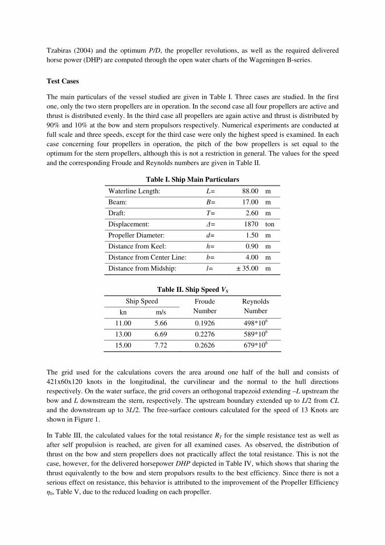
Tzabiras (2004) and the optimum P/D, the propeller revolutions, as well as the required delivered

horse power (DHP) are computed through the open water charts of the Wageningen B-series.

Test Cases

The main particulars of the vessel studied are given in Table I. Three cases are studied. In the first

one, only the two stern propellers are in operation. In the second case all four propellers are active and

thrust is distributed evenly. In the third case all propellers are again active and thrust is distributed by

90% and 10% at the bow and stern propulsors respectively. Numerical experiments are conducted at

full scale and three speeds, except for the third case were only the highest speed is examined. In each

case concerning four propellers in operation, the pitch of the bow propellers is set equal to the

optimum for the stern propellers, although this is not a restriction in general. The values for the speed

and the corresponding Froude and Reynolds numbers are given in Table II.

Table I. Ship Main Particulars

Waterline Length: L= 88.00 m

Beam: B= 17.00 m

Draft: T= 2.60 m

Displacement: ∆= 1870 ton

Propeller Diameter: d= 1.50 m

Distance from Keel: h= 0.90 m

Distance from Center Line: b= 4.00 m

Distance from Midship: l= ± 35.00 m

Table II. Ship Speed VS

Ship Speed

kn m/s

Froude

Number

Reynolds

Number

11.00 5.66 0.1926 498*106

13.00 6.69 0.2276 589*106

15.00 7.72 0.2626 679*106

The grid used for the calculations covers the area around one half of the hull and consists of

421x60x120 knots in the longitudinal, the curvilinear and the normal to the hull directions

respectively. On the water surface, the grid covers an orthogonal trapezoid extending –L upstream the

bow and L downstream the stern, respectively. The upstream boundary extended up to L/2 from CL

and the downstream up to 3L/2. The free-surface contours calculated for the speed of 13 Knots are

shown in Figure 1.

In Table III, the calculated values for the total resistance RT for the simple resistance test as well as

after self propulsion is reached, are given for all examined cases. As observed, the distribution of

thrust on the bow and stern propellers does not practically affect the total resistance. This is not the

case, however, for the delivered horsepower DHP depicted in Table IV, which shows that sharing the

thrust equivalently to the bow and stern propulsors results to the best efficiency. Since there is not a

serious effect on resistance, this behavior is attributed to the improvement of the Propeller Efficiency

η0, Table V, due to the reduced loading on each propeller.

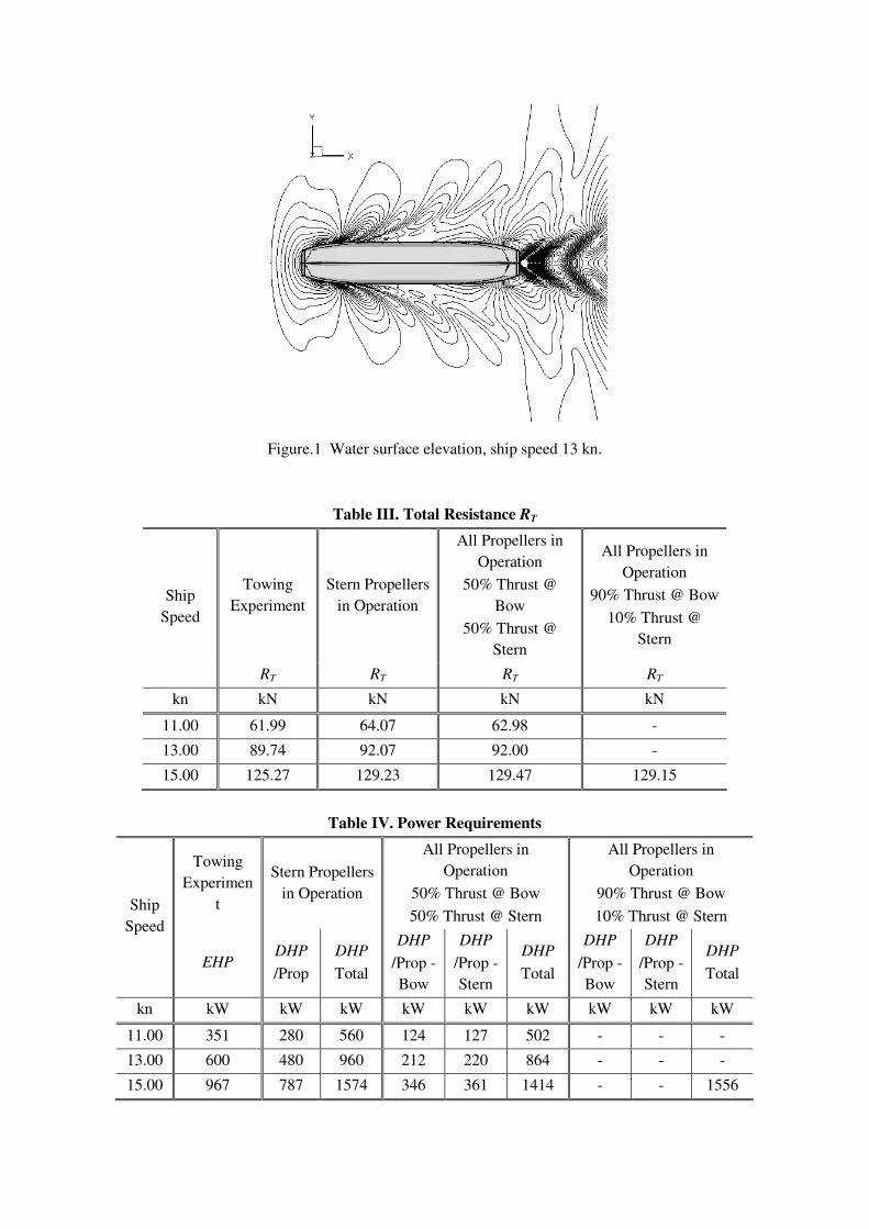
Figure.1 Water surface elevation, ship speed 13 kn.

Table III. Total Resistance RT

Towing

Experiment

Stern Propellers

in Operation

All Propellers in

Operation

50% Thrust @

Bow

50% Thrust @

Stern

All Propellers in

Operation

90% Thrust @ Bow

10% Thrust @

Stern

Ship

Speed

RT RT RT RT

kn kN kN kN kN

11.00 61.99 64.07 62.98 -

13.00 89.74 92.07 92.00 -

15.00 125.27 129.23 129.47 129.15

Table IV. Power Requirements

Towing

Experimen

t

Stern Propellers

in Operation

All Propellers in

Operation

50% Thrust @ Bow

50% Thrust @ Stern

All Propellers in

Operation

90% Thrust @ Bow

10% Thrust @ Stern Ship

Speed

EHP DHP

/Prop

DHP

Total

DHP

/Prop -

Bow

DHP

/Prop -

Stern

DHP

Total

DHP

/Prop -

Bow

DHP

/Prop -

Stern

DHP

Total

kn kW kW kW kW kW kW kW kW kW

11.00 351 280 560 124 127 502 - - -

13.00 600 480 960 212 220 864 - - -

15.00 967 787 1574 346 361 1414 - - 1556

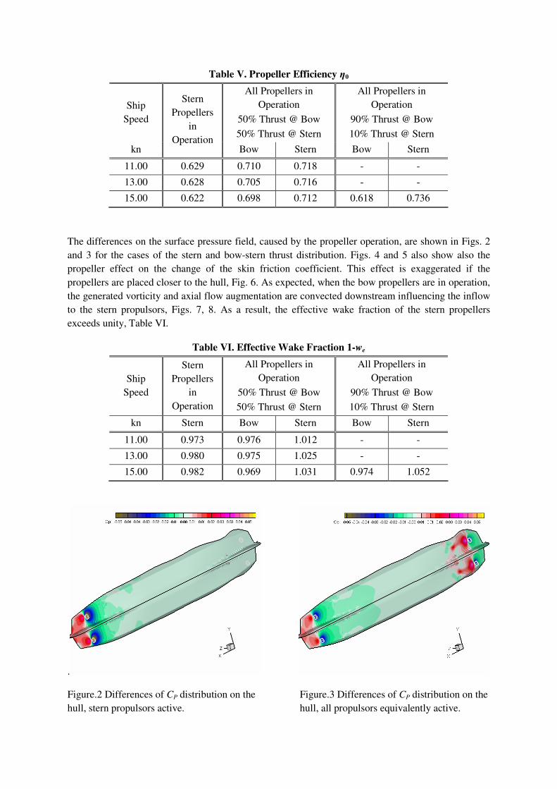
Table V. Propeller Efficiency η0

Ship

Speed

All Propellers in

Operation

50% Thrust @ Bow

50% Thrust @ Stern

All Propellers in

Operation

90% Thrust @ Bow

10% Thrust @ Stern

kn

Stern

Propellers

in

Operation Bow Stern Bow Stern

11.00 0.629 0.710 0.718 - -

13.00 0.628 0.705 0.716 - -

15.00 0.622 0.698 0.712 0.618 0.736

The differences on the surface pressure field, caused by the propeller operation, are shown in Figs. 2

and 3 for the cases of the stern and bow-stern thrust distribution. Figs. 4 and 5 also show also the

propeller effect on the change of the skin friction coefficient. This effect is exaggerated if the

propellers are placed closer to the hull, Fig. 6. As expected, when the bow propellers are in operation,

the generated vorticity and axial flow augmentation are convected downstream influencing the inflow

to the stern propulsors, Figs. 7, 8. As a result, the effective wake fraction of the stern propellers

exceeds unity, Table VI.

Table VI. Effective Wake Fraction 1-we

Ship

Speed

Stern

Propellers

in

Operation

All Propellers in

Operation

50% Thrust @ Bow

50% Thrust @ Stern

All Propellers in

Operation

90% Thrust @ Bow

10% Thrust @ Stern

kn Stern Bow Stern Bow Stern

11.00 0.973 0.976 1.012 - -

13.00 0.980 0.975 1.025 - -

15.00 0.982 0.969 1.031 0.974 1.052

.

Figure.2 Differences of CP distribution on the

hull, stern propulsors active.

Figure.3 Differences of CP distribution on the

hull, all propulsors equivalently active.

Figure.4 Differences of CF distribution on the

hull, stern propulsors active.

Figure.5 Differences of CF distribution on the

hull, all propulsors equivalently active.

Figure.6 Differences of CF distribution on the hull, all propulsors equivalently active and close to hull.

Figure.7 Vorticity contours on the propeller disk,

all propulsors equivalently active.

Figure.8 Axial isowakes on the propeller disk, all

propulsors equivalently active.

Concluding Remarks

The performed numerical tests provide valuable results with respect to the propeller operation of

double-ended ferries. An important conclusion is that to achieve the most efficient performance, the

propeller loading should be equivalently distributed between the bow and stern propulsors.

References

Tzabiras, G. Politis, G. and Loukakis T. 1995. Calculations of propulsion characteristics of a tanker using different propeller models. First International Conference on Marine Technology ODRA-95, Szczecin, Poland.

Tzabiras, GD. (ed.) Prifti, A. 2001. Numerical simulation of the separated, turbulent flow past the stern of traditional fishing vessels. Advances in Fluid Mech. series, Special volume: Calculation of Complex Turbulent Flows. Southampton : CMEM : 131-166.

Tzabiras, GD. 2004. Resistance and Self-propulsion simulations for a Series-60, CB=0.6 hull at model and full scale. Ship Technology Research. 51 : 21-34.

Validation and Application of a Massively-Parallel Hydrodynamic SPH Simulation Code

Christian Ulrich and Thomas Rung

christian.ulrich@tu-harburg.de

Hamburg University of Technology (TUHH), GermanyInstitute of Fluid Dynamics and Ship Theory (M-8)

Introduction

Mesh-free Lagrangian methods, like Smoothed-Particle-Hydrodynamics (SPH) discretize the fluid rather than the domain. They are of advantage when e.g. large relative motions or free surface flows should be captured. The SPH-method is inherently unsteady and can applied to simulations dealing with multiple phases and continua.

The industrial application of SPH-codes is traditionally limited by the maximum number of particles which can be employed if the simulation is supposed to be completed within a reasonable time-to-solution. Reliable fluids-engineering simulations often rely on fairly accurate discretizations, leading to large numbers of particles. The discretization effort increases with the complexity of the computed geometry and the involved physics (e.g. multiple phases or continua), as well as the need to accurately resolve local details. The only conceivable options to increase the number of particles are the efficient use of commodity-hardware ”Beowulf” clusters in conjunction with high-speed interconnects or massively parallel processing (MPP) supercomputers. The paper is concerned with a data-parallel SPH-procedure which is designed to simulate weakly-compressible, viscous engineering flows following Monaghan’s SPH-formalism [1]. The employed SPH-code is an immediate modification of the cosmological simulation code GADGET-2, based on the work of Springel [2]. The original procedure is devoted to hydrodynamical cosmological simulations. It follows the evolution of a self-gravitating collisionless N-body system, and allows gas dynamics to be optionally included. GADGET-2 is a data-parallel, single-programm/multiple-data (SPMD) procedure. Inter-processor communication is realized using hydrodynamic the standard Message Passing Interface (MPI) library. Unlike earlier versions of GADGET and various other particle- simulation approaches (e.g. [3]), GADGET-2 employs an efficient domain-decomposition technique. The strategy is based on the position-based mapping of particles into a space-filling curve (SFC), as proposed by Warren and Salmon [4]. Although being an ideal starting point, GADGET-2 is not directly applicable to wall-bounded fluids-engineering simulations of viscous incompressible fluids. Therefore, we adapt Springel’s parallelisation strategy to a different simulation area using modified governing equations and their respective SPH representation. We refer to the modified code as “GADGET- H2O ”. SPH-Formalism

SPH provides an integral representation of the flow field. The fluid is modeled by a finite amount of particles, carrying a mass and several field-related properties, e.g. density, pressure, velocity, temperature or turbulence energy. To evaluate the local field properties, an integrated weighted average is performed for a set of neighboring particles using a smoothing kernel function. Accordingly, the spatial derivatives of the governing transport equation (continuity, momentum, energy etc.) are evaluated analytically. The resulting system of ordinary differential equations is advanced in time, using established explicit numerical-integration schemes, e.g. Crank-Nicholson or Runge-Kutta.

This section outlines the governing equations and their respective SPH-based approximations.

Vectors and tensors are defined by reference to cartesian coordinates. The notation uses latin subscripts to identify particle locations and greek superscripts to mark cartesian tensor coordinates. The latin subscript i denotes to the focal particle whereas the subscript j refers to its neighbors. Einstein’s summation is employed over repeated Greek superscripts.

Smoothing Function

A standard cubic spline kernel function is used to perform the kernel approximation.

W r , h=8

h3 1−6 r

h 2

6 rh

3

0≤rh≤

12

2 1− rh

312

rh≤1

0 rh1

(1)

The compact-support kernel function involves the distance r=∣x i−x j

∣ between two particles and drops to zero when the particle distance approaches the kernel length h.

Conservation of Mass

The transient evolution of the density for a particle i follows from the continuity equation D i

Dt=∑

j=1

N

[m j vi−v j

]∂W ij

∂ x i (2)

where m denotes the particle mass and ρ marks the particle density. The velocity and the position of a particle refer to the vectors vβ and xβ , respectively. The kernel function around the focal particle location xi

β with respect to the neighbouring location xjβ is denoted by Wij .

Conservation of Momentum

The particle's momentum is governed by the (laminar) Navier-Stokes equation, which is approximated using the integral representation

D vi

Dt=∑

j=1

N

[m j i

i2 j

j2 ] ∂W ij

∂ xi

f i

(3)

where fiα refers to a volumetric force and σαβ denotes to the stress tensor. The latter can be split into an

isotropic pressure portion and a viscous part:i

=−p

, (4)

with the pressure p, the unity tensor δ and the viscous stress tensor ταβ . Restricting ourselves to Newtonian fluids, ταβ depends on the isotropic dynamic viscosity μ and the strain- rate tensor ɛαβ

:

=

, (5)where

=∂ v

∂ x∂ v

∂ x−

23 ∂ v

∂ x . (6)

An SPH-approximation of (5), which is suitable for single- phase simulations, reads

=1i∑j=1

N

[m j v j−v i

]∂W ij

∂ xi

1i∑j=1

N

[m j v j−vi

]∂W ij

∂ x i−[ 2

31i∑j=1

N

[m j v j−vi

]∂W ij

∂ xi ] . (7)

Several different approaches for the viscosity evaluation have been evaluated by Gonzáles et al. [5]. They conclude that the different models produce sufficient similar results. In our code, modifications [6] of the above described SPH-formulations are available at the users choice.

Multiple Continua

The presented code is supposed to be used for multi-physical port hydrodynamic problems where interactions of fluid and granular material are involved. A simple approach for the description of granular material can be formulated considering the material as a Newtonian fluid with variable viscosity. That viscosity is dependent on the internal angle of friction Ф, pressure p and the strain- rate tensor ɛαβ:

=p⋅sin

2 [kk2 ]. (8)

A similar approach was used in [7] for the simulation of granular landslides.

Equation of State

The present effort is primarily concerned with incompressible water flows. The computation of the pressure field in an incompressible fluid poses a challenge to classical SPH- simulations using an explicit time-stepping technique. In the present study, the flow is considered weakly compressible. Accordingly, Tait’s pressure-density relation [8] with the generally recommended exponent γ = 7 is used:

p= 0

−1B (9)

with a reference density ρ0 and a reference pressure B. To consider the fluid as incompressible, the density variations should be smaller than 1%. This can be ensured by a correct choice of B.

Parallelization Strategy

The parallelization is based on sorting all particles into a global space-filling Peano-Hilbert curve. This sorting ensures that a particle list is established where particles which are located close to each other in the global domain stay close in the list. One advantage of using the sorting is that the governing neighbor interactions of the SPH-methodology can be evaluated with a minimum amount of particle information from other domains. Another benefit is that the Peano-Hilbert ordering is related to cache optimization. Particles might find most of their nearest neighbors in the same cache line. Therefore, the code balance is significantly improved by the Peano-Hilbert ordering. As illustrated in figure 1, the global curve is chopped into pieces. The different parts are associated to the processors.

Figure 1: 2D Illustration of the parallelization strategy: All particles are mapped into a global space-filling curve (a). The curve is chopped into pieces. The resulting domains are associated to the different processors (b). Local BH-oct-trees are established on the processors for neighbor search (c). Neighboring processors are included as pseudo particles.

The nearest neighbor search is based on a Barnes & Hut (BH) oct-tree concept [9]. On each processor, a (local) BH-tree is constructed, where all local particles are included as well as the neighboring particles. Those are build into the tree as “pseudo particles” which represent complete neighbor processors. Information from the different neighbor processors are collected.

#CPUs

Figure 2: Parallel performance analysis for a 40Mio particle sloshing application on HLRN2. A super linear speedup can be observed up to 256 CPUs.

The codes parallel performance was analyzed using the MPP system of the Norddeutscher Verbund für Hoch- und Höchstleistungsrechen (HLRN2). The example included refers to a sloshing-tank simulation using 40Mio particles. As illustrated in figure 2, a super linear speedup can be observed.

Validation

This section gives an overview of validation examples and possible applications. An axissymmetric Couette-Flow is simulated for the validation of the viscous implementation and the moving-wall model. As illustrated in figure 3, the example refers to two co-axial cylinders with a fluid located in between. The cylinders with different radii rotate with different angular velocities. The transmission of viscous forces from the wall induces a rotating shear-flow.

Figure 3: Axissymmetric Couette-Flow as validation for viscous flows and wall-model comparison. General setup (left): Two moving cylinders with encased viscous fluid. Different boundary configurations are testet (center). Analytical and computed velocity profiles of the shear driven viscous flow (right).

The simulations are carried out with two different wall configurations. Multiple wall rows are evaluated against a single row. As displayed in figure 3, the multi wall results are closer to an analytical solution of the problem then the single wall. Generally, both configurations match the analytics quite well.

Iglesias et al. [10] have published comprehensive studies on SPH-simulations of generic, passive anti-roll tanks. Simulations as well as experimental data are available from these studies. Accordingly, an example given in [10] has been used to further validate the present GADGET- H2O implementation. The case is also used to subsequently elucidate the scalability of the present algorithm (as described in section Parallelization Strategy). Figure 4 shows snapshots from the simulation at different timesteps. The visual comparison of GADGET- H2O 's results to the ones described in [10] shows a good agreement of both simulations.

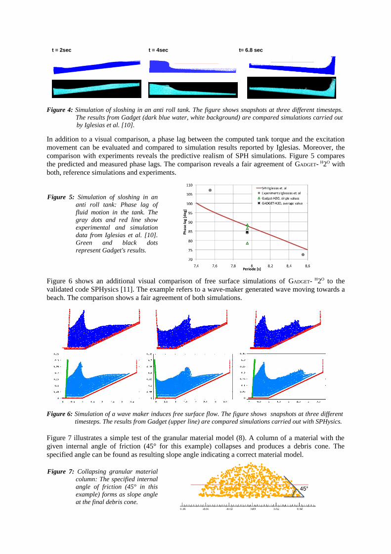
t = 2sec t = 4sec t= 6.8 sec

Figure 4: Simulation of sloshing in an anti roll tank. The figure shows snapshots at three different timesteps.

The results from Gadget (dark blue water, white background) are compared simulations carried out by Iglesias et al. [10].

In addition to a visual comparison, a phase lag between the computed tank torque and the excitation movement can be evaluated and compared to simulation results reported by Iglesias. Moreover, the comparison with experiments reveals the predictive realism of SPH simulations. Figure 5 compares the predicted and measured phase lags. The comparison reveals a fair agreement of GADGET- H2O with both, reference simulations and experiments.

Figure 5: Simulation of sloshing in an anti roll tank: Phase lag of fluid motion in the tank. The gray dots and red line show experimental and simulation data from Iglesias et al. [10]. Green and black dots represent Gadget's results.

Figure 6 shows an additional visual comparison of free surface simulations of GADGET- H2O to the validated code SPHysics [11]. The example refers to a wave-maker generated wave moving towards a beach. The comparison shows a fair agreement of both simulations.

Figure 6: Simulation of a wave maker induces free surface flow. The figure shows snapshots at three different timesteps. The results from Gadget (upper line) are compared simulations carried out with SPHysics.

Figure 7 illustrates a simple test of the granular material model (8). A column of a material with the given internal angle of friction (45° for this example) collapses and produces a debris cone. The specified angle can be found as resulting slope angle indicating a correct material model.

Figure 7: Collapsing granular material column: The specified internal angle of friction (45° in this example) forms as slope angle at the final debris cone.

Conclusion

The paper reports on the application of the parallel SPH-code GADGET- H2O for simulations of engineering hydrodynamic flows. The code is a modification of the cosmological code GADGET- 2 by Springel [2] for weakly compressible, viscous, wall-bounded fluids.

The validation examples show that the code is generally capable of simulating such types of flow phenomena. A fair agreement with analytical velocity profiles has been achieved for a viscous driven, axissymmeric Couette-flow. Results of a sloshing simulation for an anti-roll tank are in line with experimental and computational data. Basic tests for a granular material model show promising results. Uncertainties have been observed in conjunction with the modeling of walls. Accordingly, the evaluation and implementation of different wall models, capable to handle multiple continua, is an important future topic.

The procedure is designed to cope with large numbers of particles of the order of 107 − 108. It aims to extent the predictive realms of serial SPH-simulations to industrial applications. The speed-up investigation reveals a satisfactory scalability of the procedure.

A primary focus of future efforts is to incorporate an automated pre-processor for the geometry import and the initialization of particles for complex applications with minimal user input. More work will be devoted to an improved pressure-evaluation in incompressible flows. The extension to multi-physics, where special emphasis will be given to soil-fluid interaction, will be enhanced and a body- force propulsor model will be developed.

Acknowledgement

The authors would like to thank the German Research Foundation (Deutsche Forschungsgemeinschaft, DFG) for supporting the project. The present work forms part of the Research Training Group Harbours for Container Ships of Future Generations: Interaction of Ship, Fluid, Structure and Soil (GRK 1096) at the Hamburg Univ. of Technology. We greatly acknowledge the support by the Norddeutscher Verbund für Hoch- und Höchstleistungsrechnen for granting access to the MPP SGI-Altix HLRN2-supercomputer.

References

[1] Monaghan, J. J. (1994). Simulating Free Surface Flows with SPH. Journal of Computational Physics, 110:399–406

[2] Springel, V. (2005). The cosmological simulation code GADGET-2. MNRAS, 364:1105–1134

[3] Dubinski, J. (1996). A Parallel Tree Code. New Astronomy, 1:133–147

[4] Warren, M. S. and Salmon, J. K. (1993). A Parallel Hashed Oct-Tree N-Body Algorithm. Proceedings of Supercomputing ’93

[5] Gonzáles, L.M., Sánchez, J.M., Macià, F., Souto-Iglesias, A. (2009). Analysis of WCSPH laminar viscosity models. Proceedings of the 4th international SPHERIC workshop, Nantes, France

[6] Lui , G.R. and Lui, M.B. (2003). Smoothed Particle Hydrodynamics - a meshfree particle method. World Scientific Publishing Co. Pte. Ltd., Singapore

[7] Falappi, S., Gallati, M. (2007). SPH simulation of water wave generated by granular landslides. Proceedings of the 32th Congress of IAHR, Venice 933:1-10. IAHR, Madrid

[8] R. H. Cole (1948). Underwater Explosions. Princeton University Press

[9] Barnes, J. and Hut, P. (1986 ). A hierarchical O(N log N) force-calculation algorithm. Nature, 324:446–449

[10] Souto Iglesias, A., Pérez Rojas, L., and Zamora Rodr guez, R. (2003). Simulation of anti-roll tanks and sloshing type problems with smoothed particle hydrodynamics. Ocean Engineering, 31:1169–1192

[11] Gesteira, M.G., Rogers, B.D., Dalrymple, R.A. , Crespo, A.J.C., Narayanaswamy, M. (2008). User Guide for the SPHysics code.

CFD CALCULATIONS ON A CAVITATING HYDROFOIL WITH OPENFOAM

Diego Villa & Stefano Brizzolara

diego.villa@unige.it brizzolara@dinav.unige.it

Marine CFD Group, University of Genova, Italy

INTRODUCTION In the last years, with the increase of the computational capability, new CFD techniques have been applied for a lot of engineering applications. RANS solvers are one of these new techniques: in the past they were just a research instrument because of their really high computational costs, both in terms of memory occupation and computational time. Nowadays RANS has become an important business in the engineer fields, so a lot of commercial software were born to solve a general purpose CFD problems. That generated two important phenomena: on one side the RANS techniques have been applied in a lot of engineering problems, that product a lot of validation, with a systematic comparison between new developed algorithm and experimental results; on the other hand the cores of these software became a black-box for the users, and in many cases for the research centre, as the university, that couldn’t study and improve these codes. For commercial reasons these software, to be general purpose, implements only old schemes and algorithms, so the science community begun to develop open application and libraries to create a new standard for the CFD calculation. In our University an extensive development of in-house software was made in the past, generally with the potential approximation, as BEM software or Vortex Lattice methods, to solve the principal naval problems, as the numerous publications demonstrate. In parallel to this topic an extensive validation of a commercial RANS software has been carried on in a lot of standard and off-standard naval problems. Now we decided to use an open source application to validate it and to develop new specific naval problem solvers, preferably with a simple interface and using all the facilities that the CFD community gives. In this paper we present the first application of the OpenFOAM, an open source software, to an important naval problem, the cavitation generated by 2D hydrofoils.

GEOMETRY AND TEST DATA To test the OpenFOAM software, we decided to use the experimental results public by Leroux et al. 2001 that present the pressure coefficient distribution on the so call NACA66-12% profile, in a no cavitation regime and for different cavitation number. In that paper they didn’t give the geometry that can be found in a previous publication of the same institute (Astolfi et al. 2000). In the table 1 we present the profile in term of adimensional coordinates refer to the chord. In figure 1 is shown the geometry. The simulation has been performed for an angle of attack of 6 degrees and a Reynolds number of 0.8x10-6 . As well known a lot of the RANS solver, as the solver implemented in OpenFOAM, use a dimensional approach, so we tested the same chord length used for the experimental results of 100 mm.

−0.200.20

0.1

0.2

0.3

0.4

0.5

0.6

0.7

0.8

0.9

1

y/c

x/c

x* y* Suction side x* y* Pressure side0,00E+00 0,00E+00 0,00E+00 0,00E+00

-8,43E-05 8,88E-04 1,68E-04 -8,74E-04

-8,55E-05 1,79E-03 4,18E-04 -1,73E-03

-3,41E-06 2,70E-03 7,52E-04 -2,58E-03

1,62E-04 3,63E-03 1,17E-03 -3,41E-03

4,10E-04 4,58E-03 1,67E-03 -4,23E-03

7,42E-04 5,53E-03 2,25E-03 -5,03E-03

1,16E-03 6,50E-03 2,92E-03 -5,81E-03

1,65E-03 7,49E-03 3,67E-03 -6,59E-03

2,23E-03 8,48E-03 4,50E-03 -7,34E-03

2,90E-03 9,49E-03 5,41E-03 -8,09E-03

3,57E-03 1,01E-02 6,23E-03 -8,47E-03

5,87E-03 1,23E-02 8,83E-03 -1,00E-02

1,06E-02 1,58E-02 1,39E-02 -1,23E-02

2,26E-02 2,23E-02 2,64E-02 -1,61E-02

4,69E-02 3,16E-02 5,12E-02 -2,09E-02

7,13E-02 3,87E-02 7,57E-02 -2,44E-02

9,58E-02 4,46E-02 1,00E-01 -2,71E-02

1,45E-01 5,42E-02 1,49E-01 -3,12E-02

1,94E-01 6,17E-02 1,98E-01 -3,43E-02

2,43E-01 6,74E-02 2,47E-01 -3,64E-02

2,93E-01 7,18E-02 2,96E-01 -3,80E-02

3,42E-01 7,51E-02 3,44E-01 -3,90E-02

3,91E-01 7,72E-02 3,93E-01 -3,94E-02

4,41E-01 7,82E-02 4,42E-01 -3,94E-02

4,90E-01 7,80E-02 4,90E-01 -3,88E-02

5,39E-01 7,66E-02 5,39E-01 -3,75E-02

5,89E-01 7,39E-02 5,88E-01 -3,55E-02

6,38E-01 7,01E-02 6,36E-01 -3,31E-02

6,87E-01 6,49E-02 6,85E-01 -3,00E-02

7,37E-01 5,84E-02 7,34E-01 -2,66E-02

7,86E-01 5,03E-02 7,82E-01 -2,28E-02

8,35E-01 4,03E-02 8,31E-01 -1,91E-02

8,84E-01 2,90E-02 8,81E-01 -1,50E-02

9,32E-01 1,68E-02 9,30E-01 -1,01E-02

9,56E-01 1,04E-02 9,55E-01 -7,17E-03

9,81E-01 3,91E-03 9,80E-01 -3,91E-03

1,00E+00 -1,18E-03 1,00E+00 -1,18E-03 Figure 1- Geometry profile

Table 1- Adimensional coordinate of the NACA66 foil section

MESH SET-UP The OpenFOAM library doesn’t support yet advanced mesh generator, only in the last release it has been developed a snappyHexMesh to generate complex cardinal mesh, so we decided to find an open mesh generator, the GMSH. GMSH is a free/open tetrahedral/prism mesh generator, with a lot of feature to improve the quality of the generating mesh. This software present a well done Graphical User Interface (GUI) and a Text file to generate the input geometry, so we implement this software in our GUI to speed up the time to build an OpenFOAM case. Figures 2 and 3 show the mesh used for the simulation: we used an un-structured mesh compound principally of triangle cells, and we create a prism layer near the wall of quadrilateral cells. The mesh obtained for the cavitating case is made of about 12K cells, where about 28% of these are in the prism layer, that to have a good prediction of the lamina cavitation developed on the profile. Figure 4 presents the extended area of prismatic cells used near the hydrofoil.

Figure 2 – Mesh typology

Figure 3 – Detail of the prism layer near the profile

This mesh guarantee an Y+ with a maximum value of about 50 and a mean value on the suction side of the hydrofoil of less than 20. This value has been evaluated in good agreement with the ones required for the wall function approach.

OPENFOAM SOLVERS There are a lot of solvers release by the OF community: for our case we used two different solvers. The first one is a single phase RANS solver named turbulentFoam: this solver implements an un-steady approach with a PISO iterator to make the pressure-velocity linkage, and it has been performed with the Realizable k-ε model to simulate the turbulent effects. This solver, for its good stability, has been used to find the solution in the no cavitating condition. The public version of this solver has been modified to implement the time step chancing in accord with the maximum Courant number. As well known, the Courant number is a parameter that guarantees the solution stability and the no-linear approximation, and using a constant time step implies the use of a very small time discretization to grant the convergence of the solution in the fist part of the simulation, that because the initial fields are setup as constant value for each cells. When the simulation star to run, high gradient are product and the solution become stable only for very small time step. This implicate that the total time to reach the convergence of the problem is very long. Using a variable time step instead, the time machine has been reduced to the optimal one, without having an unstable solution. The second solver used during this works, is a double phase RANS solver with a Cavitation model named rasCavitatingFoam. This solver has the same characteristics of the previous one, but it uses a Interface-Capturing method, Volume of Fluids (VoF), to find the interface between the two phases. Moreover a linear barotropic compressibility model is used. The saturation pressure for the water vapour has been set at 2334 N/m2 than the ambient pressure has been changed to realize the Cavitation number expected. As well as for the no cavitating simulation, a dynamic time step has been used, but for this type of simulation two parameters have been checked: the Courant number and the Acoustic Courant number, that it is similar to the previous one but uses the mean sound velocity given as a linear combination of the sound velocity of the two phases related to the VoF value into each cell. To visualize the fields we use ParaView.

GRAPHICAL USER INTERFACE A very important part of this project was the generation of a GUI. To perform a complete simulation like this one, in a normal way, it is necessary a lot of time, in particular the major time is spent to generate the geometry, for example in a CAD, and to export it in a mesh generator and so on. Like a lot of software house made, we decided to spend part of the time to optimize the whole process, but for a particular case, so the result is that to generate a complete case ready to be solved, we spent just few minutes. Figure 4 present a sketch of the our GUI made in JAVA.

Figure 4- Sketch of the GUI developed for the Cavitation

problem.

RESULTS To check the validity of this code, a first validation for no cavitating condition has been made. The results in term of pressure coefficient distribution has been made by RANS solution and experimental results, and a in-house developed panel method. In figure 5 the comparison is presented.

0 0.1 0.2 0.3 0.4 0.5 0.6 0.7 0.8 0.9 1−1

−0.5

0

0.5

1

1.5

2

2.5

x/c

−C

p

Figure 5 – Pressure coefficient on the hydrofoil in no

cavitating condition. Alfa 6°, Reynolds number 0.8x10-6 Figure 6 – Pressure field around the hydrofoil in no

cavitating condition

Figure 7 – Stream lines detail for no cavitating condition Figure 8 – Velocity field around the hydrofoil in no

cavitating condition The RANS method gives a good agreement with the experimental data; Figures 6 and 8 show the pressure and velocity fields around the hydrofoil. In particular figure 7 present the stream lines around the profile and it’s evident that separation does not occur. After that, other three simulations in cavitating condition were performed, with different Cavitation numbers, respectively 1.41, 1.34 and 1.3. Figures 9,11 and 13 show the comparison, in term of pressure coefficient, between the panel and RAS method and the experimental results. Figure 10,12 and 14 show the shape of the bubble simulate, in the OF.

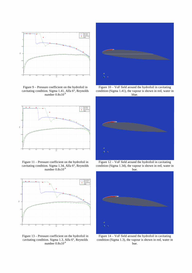
0 0.1 0.2 0.3 0.4 0.5 0.6 0.7 0.8 0.9 1−1.5

−1

−0.5

0

0.5

1

1.5

x/c

−C

p

Rans FaceRans BackExperimentalPanel

Figure 9 – Pressure coefficient on the hydrofoil in

cavitating condition. Sigma 1.41, Alfa 6°, Reynolds number 0.8x10-6

Figure 10 – VoF field around the hydrofoil in cavitating condition (Sigma 1.41), the vapour is shown in red, water in

blue.

0 0.1 0.2 0.3 0.4 0.5 0.6 0.7 0.8 0.9 1−1.5

−1

−0.5

0

0.5

1

1.5

x/c

−C

p

Rans BeckRans FaceExperimentalPanel

Figure 11 – Pressure coefficient on the hydrofoil in cavitating condition. Sigma 1.34, Alfa 6°, Reynolds

number 0.8x10-6

Figure 12 – VoF field around the hydrofoil in cavitating condition (Sigma 1.34), the vapour is shown in red, water in

bue.

0 0.1 0.2 0.3 0.4 0.5 0.6 0.7 0.8 0.9 1−1.5

−1

−0.5

0

0.5

1

1.5

x/c

−C

p

Ranse BeckRans FaceExperimentaldata4

Figure 13 – Pressure coefficient on the hydrofoil in cavitating condition. Sigma 1.3, Alfa 6°, Reynolds

number 0.8x10-6

Figure 14 – VoF field around the hydrofoil in cavitating condition (Sigma 1.3), the vapour is shown in red, water in

bue.

As shown in the graphics, the length of the cavitation bubble, calculated via the RANS solvers, is smaller than the one predicted by the panel method and by the experimental result. For high value of cavitation number, the experimental results seem not so good, because a lot of experimental tests, like Sakoda et al.(2001), show that at the trailing edge of the cavitation bubble, a pressure jump is induced, if the shape of the bubble is stable. Both the Panel and the RANS methods predicts that effect for the all the simulation. But the shape of the pressure distribution given by the experimental doesn’t present this particular shape of pressure distribution, that increase with the cavitation number. That could be due to the beginning of the detach of the cavitation bubble from the hydrofoil. However the RANS code predict a stable bubble smaller than the real one, this effect will be studied in further works.

CONCLUSION AND FURTHER PROSPECT This software has a lot of potentiality and, in junction with an accurate planning of the software development, it can be a powerful instrument for the research and for the CFD application in the Naval context. As for the particular problem studied in this paper, the OpenFOAM gives good results, in term of pressure distribution on the hydrofoil and fields around it, for the no cavitating condition. For the cavitating condition the results present some problem in terms of cavitation length, but the distribution seams accurate, in terms of bubble geometry and its effects on the pressure distribution on the hydrofoil. However a more accurate study will be made to validity, the software and its cavitation model.

ACKNOWLEDGMENT The panel method was developed and employed into the department of naval architecture and marine technologies, by Stefano Gaggero a PhD student of the University of Genova.

REFERENCE Jean-Baptiste Leroux, Andrea Astolfi and Jean-Yves Billard “An experimental investigation of partial cavitation on a two-dimensional hydrofoil” Proceedings of CAV2001 L.-A. Astolfi, J.-B. Leroux, P.Dorage, J.-Y. Billard, F.Deniset and S.de La Fuente “An experimental investigation of Cavitation Inception and Development on a two-dimensional Hydrofoil” Journal of Ship Research, Vol.44 No.4 Dec.2000 pp.259-269 Motoyuki Sakoda, Ryo Yahushji, Masatsugu Maeda and Hajime Yamaguchi ”Mechanism of cloud cavitation generation on a 2-D hydrofoil” Proceedings of CAV2001

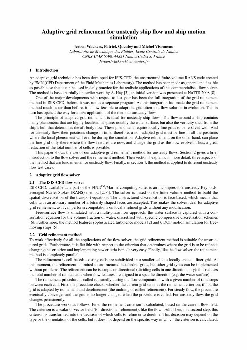
Adaptive grid refinement for unsteady ship flow and ship motionsimulation

Jeroen Wackers, Patrick Queutey and Michel VisonneauLaboratoire de Mecanique des Fluides, Ecole Centrale de Nantes

CNRS-UMR 6598, 44321 Nantes Cedex 3, FranceJeroen.Wackers@ec-nantes.fr

1 Introduction

An adaptive grid technique has been developed for ISIS-CFD, the unstructured finite-volume RANS code createdby EMN (CFD Department of the Fluid Mechanics Laboratory). The method has been made as general and flexibleas possible, so that it can be used in daily practice for the realistic applications of this commercialised flow solver.The method is based partially on earlier work by A. Hay [3], an initial version was presented at NuTTS 2008 [8].

One of the major developments with respect to last year has been the full integration of the grid refinementmethod in ISIS-CFD; before, it was run as a separate program. As this integration has made the grid refinementmethod much faster than before, it is now feasible to adapt the grid often to a flow solution in evolution. This inturn has opened the way for a new application of the method: unsteady flows.

The principle of adaptive grid refinement is ideal for unsteady ship flows. The flow around a ship containsmany phenomena that are highly localised in space: notably the water surface, but also the vorticity shed from theship’s hull that determines the aft-body flow. These phenomena require locally fine grids to be resolved well. Andfor unsteady flow, their positions change in time; therefore, a non-adapted grid must be fine in all the positionswhere the local phenomena will ever be during the simulation. Adaptive refinement, on the other hand, can placethe fine grid only there where the flow features are now, and change the grid as the flow evolves. Thus, a greatreduction of the total number of cells is possible.

This paper shows the use of our adaptive grid refinement method for unsteady flows. Section 2 gives a briefintroduction to the flow solver and the refinement method. Then section 3 explains, in more detail, three aspects ofthe method that are fundamental for unsteady flow. Finally, in section 4, the method is applied to different unsteadyflow test cases.

2 Adaptive grid flow solver

2.1 The ISIS-CFD flow solverISIS-CFD, available as a part of the FINETM/Marine computing suite, is an incompressible unsteady Reynolds-averaged Navier-Stokes (RANS) method [2, 6]. The solver is based on the finite volume method to build thespatial discretisation of the transport equations. The unstructured discretisation is face-based, which means thatcells with an arbitrary number of arbitrarily shaped faces are accepted. This makes the solver ideal for adaptivegrid refinement, as it can perform computations on locally refined grids without any modification.

Free-surface flow is simulated with a multi-phase flow approach: the water surface is captured with a con-servation equation for the volume fraction of water, discretised with specific compressive discretisation schemes[6]. Furthermore, the method features sophisticated turbulence models [2] and 6 DOF motion simulation for free-moving ships [5].

2.2 Grid refinement methodTo work effectively for all the applications of the flow solver, the grid refinement method is suitable for unstruc-tured grids. Furthermore, it is flexible with respect to the criterion that determines where the grid is to be refined:changing this criterion and implementing new criteria is made very easy. Finally, like the flow solver, the refinementmethod is completely parallel.

The refinement is cell-based: existing cells are subdivided into smaller cells to locally create a finer grid. Atthis moment, the refinement is limited to unstructured hexahedral grids, but other grid types can be implementedwithout problems. The refinement can be isotropic or directional (dividing cells in one direction only): this reducesthe total number of refined cells when flow features are aligned in a specific direction (e.g. the water surface).

The refinement procedure is called repeatedly during the flow computation, with a given number of time stepsbetween each call. First, the procedure checks whether the current grid satisfies the refinement criterion; if not, thegrid is adapted by refinement and derefinement (the undoing of earlier refinement). For steady flow, the procedureeventually converges and the grid is no longer changed when the procedure is called. For unsteady flow, the gridchanges permanently.

The procedure works as follows. First, the refinement criterion is calculated, based on the current flow field.The criterion is a scalar or vector field (for directional refinement), like the flow itself. Then, in a second step, thiscriterion is transformed into the decision of which cells to refine or to derefine. This decision may depend on thetype or the orientation of the cells, but it does not depend on the specific way in which the criterion is calculated;

it is the same for all criteria. Therefore, it is very easy to change criteria. Finally, the derefinement and refinementof cells are performed where needed. Part of the refinement is the automatic load balancing: when computing inparallel, parts of the refined grid are displaced from one processor to another, to keep the total number of cells thesame on each processor. Load balancing is essential for good computational efficiency.

3 Unsteady flow special features

The refinement method is the same for steady and unsteady flow. However, some aspects of the method, thatare useful but not indispensable for steady flow, become essential when simulating unsteady flow. Three of theseaspects are described here.

3.1 DerefinementWhen following a localised flow phenomenon, the mesh refinement must be undone in the regions where the localfeature has passed, otherwise an unnecessarily fine grid will remain there. This is done with derefinement, i.e.changing a group of fine cells, that was created by dividing one large cell, back into that single large cell.

To perform derefinement, the history of the refinement is stored by adding ‘family tie’ pointers to the cells.When a cell is refined, all the new small cells get a ‘mother’ pointer to the old big cell and ‘sister’ pointers toeach other. Thus, the group can be found again later and changed back into the single large cell. The large cellis saved as a ‘dead’ cell, that has no faces nor a state vector, only family ties. Thus, it remembers its own sistersand mother (probably ‘dead’ as well), in case it has to be derefined itself, after being restored. Apart from the cellfamily ties, no history information is needed. The faces and nodes of the large cells can be reconstructed with justthe information on the cells.

3.2 Face-cell alignmentAn important region for automatic grid refinement is near the water surface. Here, the volume fraction, that dis-tinguishes between water and air, is a numerical discontinuity; the accurate solution of its convection equation isimportant for the overall solution quality.

The convection equation for the volume fraction is sensitive to the quality of the grid. Specifically, faces parallelto the water surface that have a large cell on one side and refined small cells on the other (see figure 1a) cause adistortion and diffusion of the water surface. This distortion appears, because the discretisation of convective fluxesat the faces becomes less accurate when there is a strong misalignment between the lines that connect a face centrewith the centres of its two neighbour cells [6]. For steady flow this is no major problem, experience shows that thecompressive discretisation downstream of the bad face regularises and recompresses the interface. But for unsteadyflow, where the interface moves in time, the distortions remain.

a) b)

Figure 1: Grid misalignment distorts the water surface (a), the curves represent volume fraction isolines. Grid quality criterion(b): too large angles between face normals and lines cell – face are not allowed.

This problem is solved by enforcing the refinement of extra cells to keep a good grid quality. For this, a qualitycriterion is applied during the refinement decision step (figure 1b): if the refinement of the cell at one side of aface would cause too great an angle between the face normal and the line cell centre - face centre, the cell on theother side of the face is refined as well. The enforcement of this criterion gives regular grids at the water surface.Examples can be seen in section 4.

3.3 Solution prolongationWhen a cell is being refined, the flow state in the new small cells has to be set. As the refinement takes placebetween time steps, the state in the small cells at the beginning of the new time step has to be consistent withthe state in the large cells at the end of the old time step. For the incompressible Navier-Stokes equations, theconsistency constraints are the conservation of mass and momentum (and of the volume fraction, for the two-phase formulation). Conservation of momentum (and of the volume fraction) is easy to satisfy: the average ofthe momentum in a group of new cells must be equal to the momentum in the original large cell. This implies aconstraint on the velocity.

Conservation of mass is more difficult: it requires ∇ · u = 0. ISIS-CFD uses a Rhie and Chow SIMPLE-likediscretisation for the fluxes [6]. In essence, Rhie and Chow is a pressure-velocity coupling: the fluxes in the cell

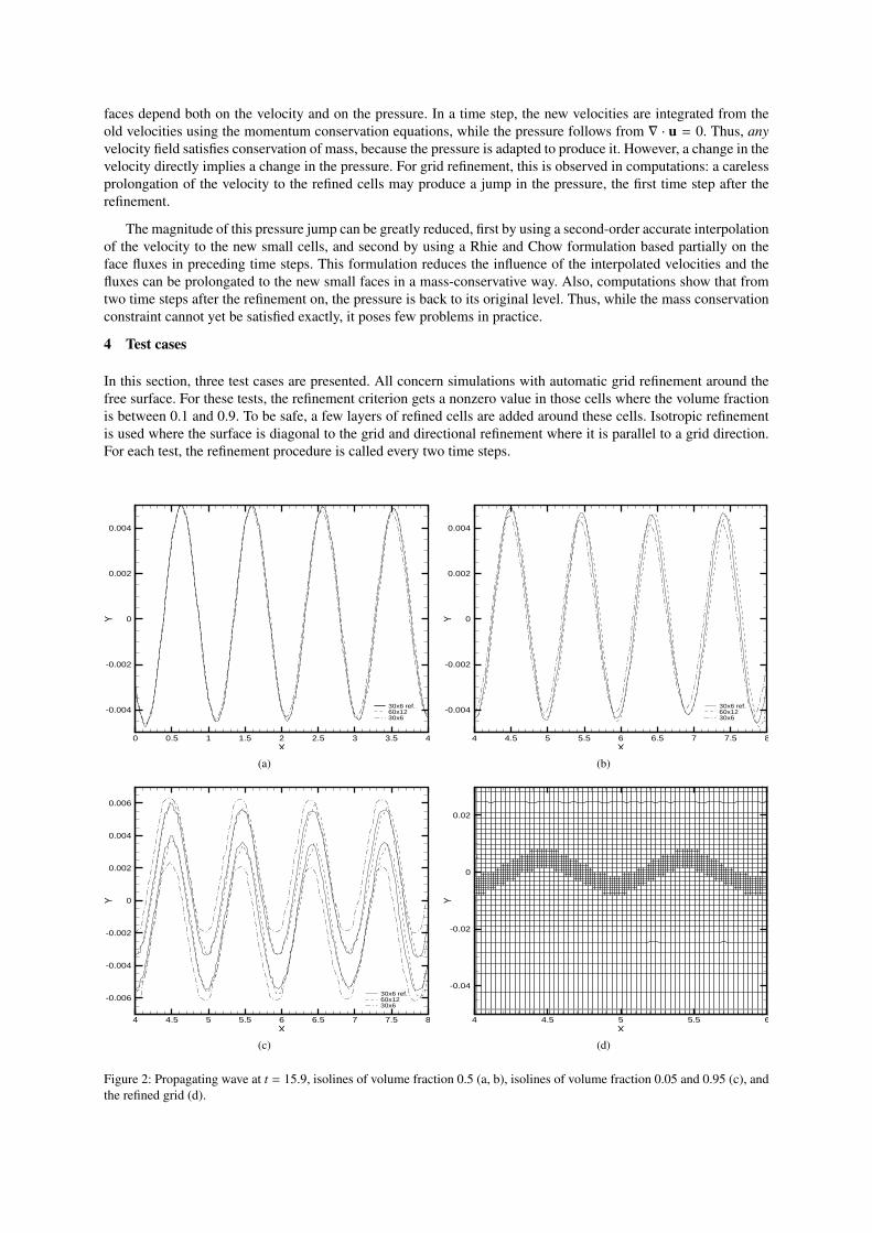
faces depend both on the velocity and on the pressure. In a time step, the new velocities are integrated from theold velocities using the momentum conservation equations, while the pressure follows from ∇ · u = 0. Thus, anyvelocity field satisfies conservation of mass, because the pressure is adapted to produce it. However, a change in thevelocity directly implies a change in the pressure. For grid refinement, this is observed in computations: a carelessprolongation of the velocity to the refined cells may produce a jump in the pressure, the first time step after therefinement.

The magnitude of this pressure jump can be greatly reduced, first by using a second-order accurate interpolationof the velocity to the new small cells, and second by using a Rhie and Chow formulation based partially on theface fluxes in preceding time steps. This formulation reduces the influence of the interpolated velocities and thefluxes can be prolongated to the new small faces in a mass-conservative way. Also, computations show that fromtwo time steps after the refinement on, the pressure is back to its original level. Thus, while the mass conservationconstraint cannot yet be satisfied exactly, it poses few problems in practice.

4 Test cases

In this section, three test cases are presented. All concern simulations with automatic grid refinement around thefree surface. For these tests, the refinement criterion gets a nonzero value in those cells where the volume fractionis between 0.1 and 0.9. To be safe, a few layers of refined cells are added around these cells. Isotropic refinementis used where the surface is diagonal to the grid and directional refinement where it is parallel to a grid direction.For each test, the refinement procedure is called every two time steps.

X

Y

0 0.5 1 1.5 2 2.5 3 3.5 4

-0.004

-0.002

0

0.002

0.004

30x6 ref.60x1230x6

(a)X

Y

4 4.5 5 5.5 6 6.5 7 7.5 8

-0.004

-0.002

0

0.002

0.004

30x6 ref.60x1230x6

(b)

X

Y

4 4.5 5 5.5 6 6.5 7 7.5 8

-0.006

-0.004

-0.002

0

0.002

0.004

0.006

30x6 ref.60x1230x6

(c)X

Y

4 4.5 5 5.5 6

-0.04

-0.02

0

0.02

(d)

Figure 2: Propagating wave at t = 15.9, isolines of volume fraction 0.5 (a, b), isolines of volume fraction 0.05 and 0.95 (c), andthe refined grid (d).

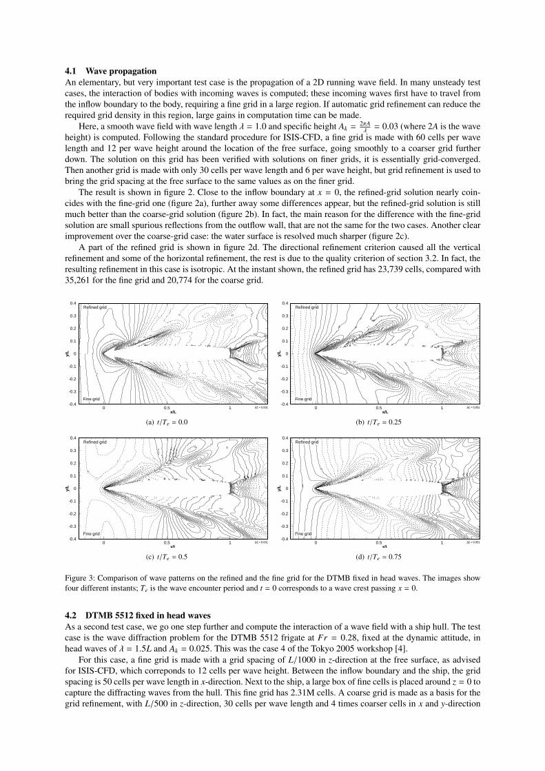
4.1 Wave propagationAn elementary, but very important test case is the propagation of a 2D running wave field. In many unsteady testcases, the interaction of bodies with incoming waves is computed; these incoming waves first have to travel fromthe inflow boundary to the body, requiring a fine grid in a large region. If automatic grid refinement can reduce therequired grid density in this region, large gains in computation time can be made.

Here, a smooth wave field with wave length λ = 1.0 and specific height Ak =2πAλ= 0.03 (where 2A is the wave

height) is computed. Following the standard procedure for ISIS-CFD, a fine grid is made with 60 cells per wavelength and 12 per wave height around the location of the free surface, going smoothly to a coarser grid furtherdown. The solution on this grid has been verified with solutions on finer grids, it is essentially grid-converged.Then another grid is made with only 30 cells per wave length and 6 per wave height, but grid refinement is used tobring the grid spacing at the free surface to the same values as on the finer grid.

The result is shown in figure 2. Close to the inflow boundary at x = 0, the refined-grid solution nearly coin-cides with the fine-grid one (figure 2a), further away some differences appear, but the refined-grid solution is stillmuch better than the coarse-grid solution (figure 2b). In fact, the main reason for the difference with the fine-gridsolution are small spurious reflections from the outflow wall, that are not the same for the two cases. Another clearimprovement over the coarse-grid case: the water surface is resolved much sharper (figure 2c).

A part of the refined grid is shown in figure 2d. The directional refinement criterion caused all the verticalrefinement and some of the horizontal refinement, the rest is due to the quality criterion of section 3.2. In fact, theresulting refinement in this case is isotropic. At the instant shown, the refined grid has 23,739 cells, compared with35,261 for the fine grid and 20,774 for the coarse grid.

x/L

y/L

0 0.5 1-0.4

-0.3

-0.2

-0.1

0

0.1

0.2

0.3

0.4

∆ξ = 0.001

Fine grid

Refined grid

(a) t/Te = 0.0x/L

y/L

0 0.5 1-0.4

-0.3

-0.2

-0.1

0

0.1

0.2

0.3

0.4

∆ξ = 0.001

Fine grid

Refined grid

(b) t/Te = 0.25

x/L

y/L

0 0.5 1-0.4

-0.3

-0.2

-0.1

0

0.1

0.2

0.3

0.4

∆ξ = 0.001

Fine grid

Refined grid

(c) t/Te = 0.5x/L

y/L

0 0.5 1-0.4

-0.3

-0.2

-0.1

0

0.1

0.2

0.3

0.4

∆ξ = 0.001

Fine grid

Refined grid

(d) t/Te = 0.75

Figure 3: Comparison of wave patterns on the refined and the fine grid for the DTMB fixed in head waves. The images showfour different instants; Te is the wave encounter period and t = 0 corresponds to a wave crest passing x = 0.

4.2 DTMB 5512 fixed in head wavesAs a second test case, we go one step further and compute the interaction of a wave field with a ship hull. The testcase is the wave diffraction problem for the DTMB 5512 frigate at Fr = 0.28, fixed at the dynamic attitude, inhead waves of λ = 1.5L and Ak = 0.025. This was the case 4 of the Tokyo 2005 workshop [4].

For this case, a fine grid is made with a grid spacing of L/1000 in z-direction at the free surface, as advisedfor ISIS-CFD, which correponds to 12 cells per wave height. Between the inflow boundary and the ship, the gridspacing is 50 cells per wave length in x-direction. Next to the ship, a large box of fine cells is placed around z = 0 tocapture the diffracting waves from the hull. This fine grid has 2.31M cells. A coarse grid is made as a basis for thegrid refinement, with L/500 in z-direction, 30 cells per wave length and 4 times coarser cells in x and y-direction

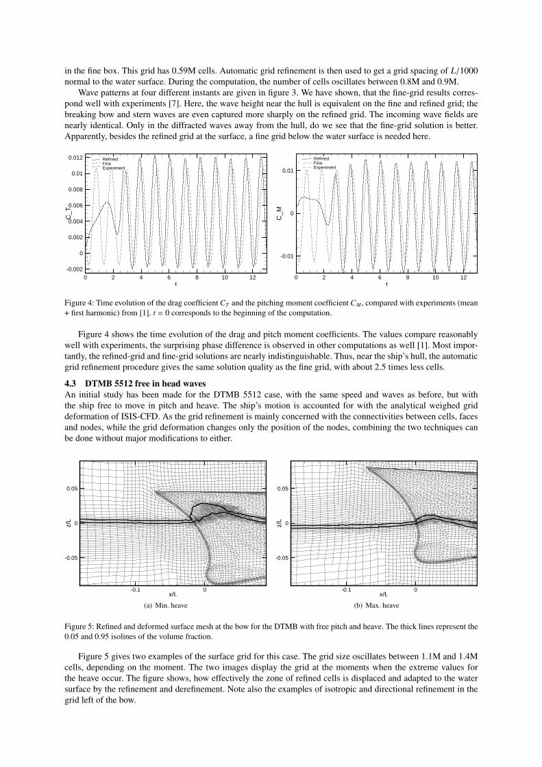
in the fine box. This grid has 0.59M cells. Automatic grid refinement is then used to get a grid spacing of L/1000normal to the water surface. During the computation, the number of cells oscillates between 0.8M and 0.9M.

Wave patterns at four different instants are given in figure 3. We have shown, that the fine-grid results corres-pond well with experiments [7]. Here, the wave height near the hull is equivalent on the fine and refined grid; thebreaking bow and stern waves are even captured more sharply on the refined grid. The incoming wave fields arenearly identical. Only in the diffracted waves away from the hull, do we see that the fine-grid solution is better.Apparently, besides the refined grid at the surface, a fine grid below the water surface is needed here.

t

C_T

0 2 4 6 8 10 12-0.002

0

0.002

0.004

0.006

0.008

0.01

0.012 RefinedFineExperiment

tC

_M0 2 4 6 8 10 12

-0.01

0

0.01

RefinedFineExperiment

Figure 4: Time evolution of the drag coefficient CT and the pitching moment coefficient CM , compared with experiments (mean+ first harmonic) from [1]. t = 0 corresponds to the beginning of the computation.

Figure 4 shows the time evolution of the drag and pitch moment coefficients. The values compare reasonablywell with experiments, the surprising phase difference is observed in other computations as well [1]. Most impor-tantly, the refined-grid and fine-grid solutions are nearly indistinguishable. Thus, near the ship’s hull, the automaticgrid refinement procedure gives the same solution quality as the fine grid, with about 2.5 times less cells.

4.3 DTMB 5512 free in head wavesAn initial study has been made for the DTMB 5512 case, with the same speed and waves as before, but withthe ship free to move in pitch and heave. The ship’s motion is accounted for with the analytical weighed griddeformation of ISIS-CFD. As the grid refinement is mainly concerned with the connectivities between cells, facesand nodes, while the grid deformation changes only the position of the nodes, combining the two techniques canbe done without major modifications to either.

x/L

z/L

-0.1 0

-0.05

0

0.05

(a) Min. heave

x/L

z/L

-0.1 0

-0.05

0

0.05

(b) Max. heave

Figure 5: Refined and deformed surface mesh at the bow for the DTMB with free pitch and heave. The thick lines represent the0.05 and 0.95 isolines of the volume fraction.

Figure 5 gives two examples of the surface grid for this case. The grid size oscillates between 1.1M and 1.4Mcells, depending on the moment. The two images display the grid at the moments when the extreme values forthe heave occur. The figure shows, how effectively the zone of refined cells is displaced and adapted to the watersurface by the refinement and derefinement. Note also the examples of isotropic and directional refinement in thegrid left of the bow.

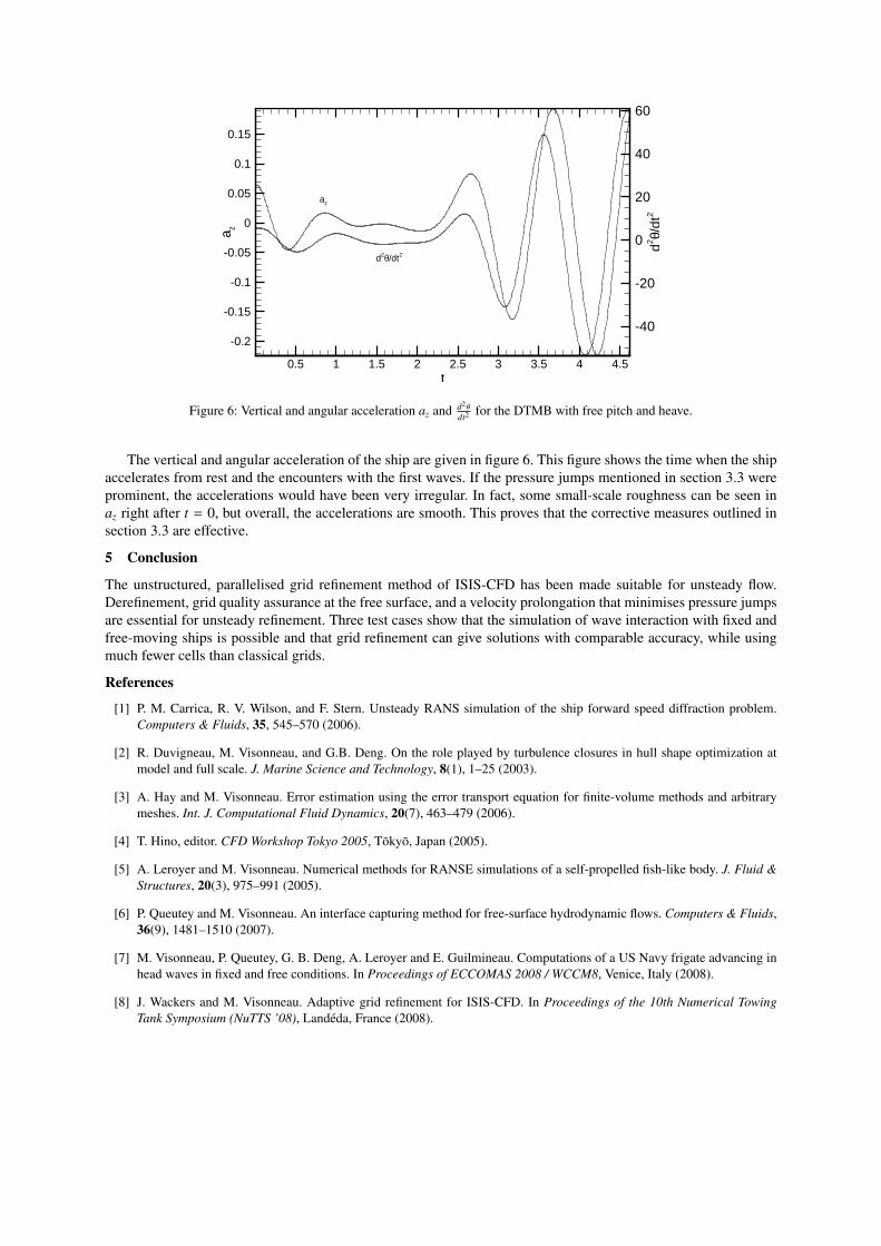
t

a z

d2 θ/dt

2

0.5 1 1.5 2 2.5 3 3.5 4 4.5

-0.2

-0.15

-0.1

-0.05

0

0.05

0.1

0.15

-40

-20

0

20

40

60

az

d2θ/dt2

Figure 6: Vertical and angular acceleration az and d2θdt2 for the DTMB with free pitch and heave.

The vertical and angular acceleration of the ship are given in figure 6. This figure shows the time when the shipaccelerates from rest and the encounters with the first waves. If the pressure jumps mentioned in section 3.3 wereprominent, the accelerations would have been very irregular. In fact, some small-scale roughness can be seen inaz right after t = 0, but overall, the accelerations are smooth. This proves that the corrective measures outlined insection 3.3 are effective.

5 Conclusion

The unstructured, parallelised grid refinement method of ISIS-CFD has been made suitable for unsteady flow.Derefinement, grid quality assurance at the free surface, and a velocity prolongation that minimises pressure jumpsare essential for unsteady refinement. Three test cases show that the simulation of wave interaction with fixed andfree-moving ships is possible and that grid refinement can give solutions with comparable accuracy, while usingmuch fewer cells than classical grids.

References

[1] P. M. Carrica, R. V. Wilson, and F. Stern. Unsteady RANS simulation of the ship forward speed diffraction problem.Computers & Fluids, 35, 545–570 (2006).

[2] R. Duvigneau, M. Visonneau, and G.B. Deng. On the role played by turbulence closures in hull shape optimization atmodel and full scale. J. Marine Science and Technology, 8(1), 1–25 (2003).

[3] A. Hay and M. Visonneau. Error estimation using the error transport equation for finite-volume methods and arbitrarymeshes. Int. J. Computational Fluid Dynamics, 20(7), 463–479 (2006).

[4] T. Hino, editor. CFD Workshop Tokyo 2005, Tokyo, Japan (2005).

[5] A. Leroyer and M. Visonneau. Numerical methods for RANSE simulations of a self-propelled fish-like body. J. Fluid &Structures, 20(3), 975–991 (2005).

[6] P. Queutey and M. Visonneau. An interface capturing method for free-surface hydrodynamic flows. Computers & Fluids,36(9), 1481–1510 (2007).

[7] M. Visonneau, P. Queutey, G. B. Deng, A. Leroyer and E. Guilmineau. Computations of a US Navy frigate advancing inhead waves in fixed and free conditions. In Proceedings of ECCOMAS 2008 / WCCM8, Venice, Italy (2008).

[8] J. Wackers and M. Visonneau. Adaptive grid refinement for ISIS-CFD. In Proceedings of the 10th Numerical TowingTank Symposium (NuTTS ’08), Landeda, France (2008).

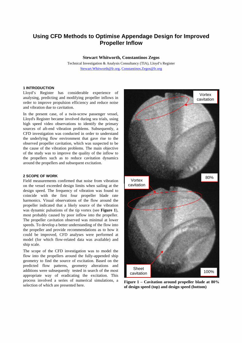
Using CFD Methods to Optimise Appendage Design for Improved Propeller Inflow

Stewart Whitworth, Constantinos Zegos

Technical Investigation & Analysis Consultancy (TIA), Lloyd’s Register Stewart.Whitworth@lr.org, Constantinos.Zegos@lr.org

1 INTRODUCTION Lloyd’s Register has considerable experience of analysing, predicting and modifying propeller inflows in order to improve propulsion efficiency and reduce noise and vibration due to cavitation. In the present case, of a twin-screw passenger vessel, Lloyd's Register became involved during sea trials, using high speed video observations to identify the primary sources of aft-end vibration problems. Subsequently, a CFD investigation was conducted in order to understand the underlying flow environment that gave rise to the observed propeller cavitation, which was suspected to be the cause of the vibration problems. The main objective of the study was to improve the quality of the inflow to the propellers such as to reduce cavitation dynamics around the propellers and subsequent excitation.

2 SCOPE OF WORK Field measurements confirmed that noise from vibration on the vessel exceeded design limits when sailing at the design speed. The frequency of vibration was found to coincide with the first four propeller blade rate harmonics. Visual observations of the flow around the propeller indicated that a likely source of the vibration was dynamic pulsations of the tip vortex (see Figure 1), most probably caused by poor inflow into the propeller. The propeller cavitation observed was minimal at lower speeds. To develop a better understanding of the flow into the propeller and provide recommendations as to how it could be improved, CFD analyses were performed at model (for which flow-related data was available) and ship scale. The scope of the CFD investigation was to model the flow into the propellers around the fully-appended ship geometry to find the source of excitation. Based on the predicted flow patterns, geometry alterations and additions were subsequently tested in search of the most appropriate way of eradicating the excitation. This process involved a series of numerical simulations, a selection of which are presented here.

Vortex cavitation

80%

Figure 1 – Cavitation around propeller blade at 80% of design speed (top) and design speed (bottom)

Vortex cavitation

Sheet cavitation 100%

3 METHODOLOGY 3.1 Computational Mesh The geometry of the ship and appendages was provided in the form of IGES files. Based on these a hexahedral “trimmed-cell” mesh was produced with mesh refinement around the hull surface and appendages. The total mesh size was around 5 million cells. Figure 2 shows a side view of the mesh on the ship surface with the refined appendages labelled.

Figure 2 – Hexahedral mesh on fully-appended hull

3.2 Modelling Approach Work was performed using STAR-CCM+ v3.06 software [1] following procedures verified in previous studies of a similar nature. To reduce computational effort several simplifications were made. Firstly, the flow was only modelled around one quarter of the ship. This was achieved by modelling only the aft half of the ship and by using a symmetry plane down the centre line. Secondly, only the part of the ship that was immersed was modelled taking advantage of the fact that the free surface was expected to have a negligible effect on the flow into and around the propellers. A symmetry boundary was placed on the flat top surface of the fluid domain, which was positioned according to the design draft at the required ship speed. The inflow field prescribed at the ship’s midpoint section was determined by performing an analysis of the flow around the complete unappended hull and extracting the necessary velocity, pressure and turbulence data. The propeller was represented by a momentum source term generated using the propeller modelling panel code PROCAL [2], which is based upon the boundary element method. Analyses were performed using both the k-ω SST and Reynolds stress turbulence models. The choice of the k-ω SST model was based on a growing body of experience, both within Lloyd’s Register and externally, suggesting that it performs better for the swirling and separating flows typically observed around ships than other two-equation eddy-viscosity models [3]. Despite this, the inherent assumption of isotropic turbulence, which linear two-equation models are based upon, means that swirling and secondary flows are always likely to be

underpredicted. For this reason, and despite the additional computational overhead and difficulties with convergence, the more complex Reynolds stress model was also used. Unless stated, all results presented here are produced using the Reynolds stress model. The solid surfaces of the hull were modelled using an ‘all y+’ wall treatment approach that emulates high y+ (wall function) and low y+ wall treatment models depending on the y+ value in the near-wall cell [1]. This approach is expected to produce better results in the near-wall region as it is suitable for use with grids that fully resolve the near-wall layer as well as those that do not. Given that the near-wall mesh used for this work was not sufficiently fine to properly resolve the viscous sublayer, the high y+ wall treatment model was likely employed along most of the walls. For all calculations the flow velocities, pressures and temperatures in the domain are calculated using the standard SIMPLE (Semi Implicit Method for Pressure Linked Equations) pressure correction method [1]. A second-order upwind differencing scheme, [1] was employed in the solution of the momentum equations and the turbulence parameters.

4 ORIGINAL GEOMETRY The results for the flow around the original geometry at full scale show a large tube vortex entering the propeller disc at around the 1 o’clock position. The wake coming off the skeg is relatively weak, however the disturbance to the flow is increased by the addition of a sheet vortex generated on the inside of the skeg and shaft, as shown in Figure 3 and Figure 4.

Figure 3 – Non-axial velocity vectors on a plane 0.216D upstream of the propeller disc centre

Propeller Disc

Sheet vortex Tube Vortex

Skeg Shaft Brackets

Pair of small counter-rotating

vortices

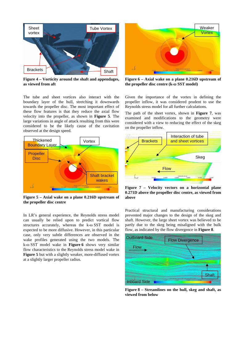
Figure 4 – Vorticity around the shaft and appendages, as viewed from aft The tube and sheet vortices also interact with the boundary layer of the hull, stretching it downwards towards the propeller disc. The most important effect of these flow features is that they reduce the axial flow velocity into the propeller, as shown in Figure 5. The large variations in angle of attack resulting from this were considered to be the likely cause of the cavitation observed at the design speed.

Figure 5 – Axial wake on a plane 0.216D upstream of the propeller disc centre In LR’s general experience, the Reynolds stress model can usually be relied upon to predict vortical flow structures accurately, whereas the k-ω SST model is expected to be more diffusive. However, in this particular case, only very subtle differences are observed in the wake profiles generated using the two models. The k-ω SST model wake in Figure 6 shows very similar flow characteristics to the Reynolds stress model wake in Figure 5 but with a slightly weaker, more-diffused vortex at a slightly larger propeller radius.

Figure 6 – Axial wake on a plane 0.216D upstream of the propeller disc centre (k-ω SST model) Given the importance of the vortex in defining the propeller inflow, it was considered prudent to use the Reynolds stress model for all further calculations. The path of the sheet vortex, shown in Figure 7, was examined and modifications to the geometry were considered with a view to reducing the effect of the skeg on the propeller inflow.

Figure 7 – Velocity vectors on a horizontal plane 0.271D above the propeller disc centre, as viewed from above Practical structural and manufacturing considerations prevented major changes to the design of the skeg and shaft. However, the large sheet vortex was believed to be partly due to the skeg being misaligned with the bulk flow, as indicated by the flow divergence in Figure 8.

Figure 8 – Streamlines on the hull, skeg and shaft, as viewed from below

Weaker Vortex

Sheet vortex

Tube Vortex

Propeller Disc

Thickened Boundary Layer

Vortex

Shaft bracket wakes

Skeg

Brackets Interaction of tube and sheet vortices

Flow Divergence

Brackets Shaft

Flow

Outboard Side

Flow

Shaft Inboard Side

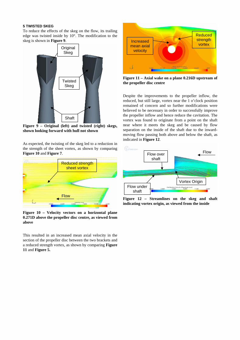
5 TWISTED SKEG To reduce the effects of the skeg on the flow, its trailing edge was twisted inside by 10°. The modification to the skeg is shown in Figure 9.

Figure 9 – Original (left) and twisted (right) skegs, shown looking forward with hull not shown As expected, the twisting of the skeg led to a reduction in the strength of the sheet vortex, as shown by comparing Figure 10 and Figure 7.

Figure 10 – Velocity vectors on a horizontal plane 0.271D above the propeller disc centre, as viewed from above This resulted in an increased mean axial velocity in the section of the propeller disc between the two brackets and a reduced strength vortex, as shown by comparing Figure 11 and Figure 5.

Figure 11 – Axial wake on a plane 0.216D upstream of the propeller disc centre Despite the improvements to the propeller inflow, the reduced, but still large, vortex near the 1 o’clock position remained of concern and so further modifications were believed to be necessary in order to successfully improve the propeller inflow and hence reduce the cavitation. The vortex was found to originate from a point on the shaft near where it meets the skeg and be caused by flow separation on the inside of the shaft due to the inward-moving flow passing both above and below the shaft, as indicated in Figure 12.

Figure 12 – Streamlines on the skeg and shaft indicating vortex origin, as viewed from the inside

Reduced strength sheet vortex

Reduced strength vortex

Increased mean axial

velocity Original

Skeg

Flow over shaft

Flow under shaft

Vortex Origin

Flow

Shaft

Twisted Skeg

Flow

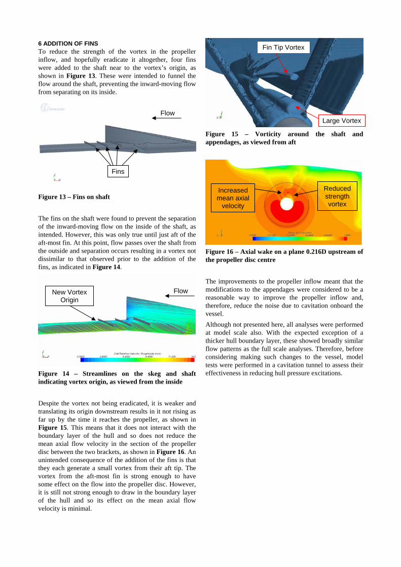
6 ADDITION OF FINS To reduce the strength of the vortex in the propeller inflow, and hopefully eradicate it altogether, four fins were added to the shaft near to the vortex’s origin, as shown in Figure 13. These were intended to funnel the flow around the shaft, preventing the inward-moving flow from separating on its inside.

Figure 13 – Fins on shaft The fins on the shaft were found to prevent the separation of the inward-moving flow on the inside of the shaft, as intended. However, this was only true until just aft of the aft-most fin. At this point, flow passes over the shaft from the outside and separation occurs resulting in a vortex not dissimilar to that observed prior to the addition of the fins, as indicated in Figure 14.

Figure 14 – Streamlines on the skeg and shaft indicating vortex origin, as viewed from the inside Despite the vortex not being eradicated, it is weaker and translating its origin downstream results in it not rising as far up by the time it reaches the propeller, as shown in Figure 15. This means that it does not interact with the boundary layer of the hull and so does not reduce the mean axial flow velocity in the section of the propeller disc between the two brackets, as shown in Figure 16. An unintended consequence of the addition of the fins is that they each generate a small vortex from their aft tip. The vortex from the aft-most fin is strong enough to have some effect on the flow into the propeller disc. However, it is still not strong enough to draw in the boundary layer of the hull and so its effect on the mean axial flow velocity is minimal.

Figure 15 – Vorticity around the shaft and appendages, as viewed from aft

Figure 16 – Axial wake on a plane 0.216D upstream of the propeller disc centre The improvements to the propeller inflow meant that the modifications to the appendages were considered to be a reasonable way to improve the propeller inflow and, therefore, reduce the noise due to cavitation onboard the vessel. Although not presented here, all analyses were performed at model scale also. With the expected exception of a thicker hull boundary layer, these showed broadly similar flow patterns as the full scale analyses. Therefore, before considering making such changes to the vessel, model tests were performed in a cavitation tunnel to assess their effectiveness in reducing hull pressure excitations.

Fins

New Vortex Origin

Flow

Flow

Fin Tip Vortex

Large Vortex

Reduced strength vortex

Increased mean axial

velocity

10 REFERENCES 7 MODEL TESTS Based on the CFD results, a twisted skeg was fitted to a model of the vessel that had been used for earlier tests and the four fins were added to the shaft. Cavitation tunnel tests were then repeated at various speeds. The results obtained at the design speed are shown in Figure 17. They show a 46% reduction in the hull pressure amplitudes at the blade passing frequency and 16%, 48%, 24% and 8% reductions in the hull pressure excitations at the next four harmonics.

1. STAR-CCM+ 3.06.006 User Guide, CD-adapco Group, 2008.

2. PROCAL v1.1 User Guide, MARIN, Dec 2007. 3. S. Whitworth, “Validation of CFD methods for Wake

Prediction”, MCS/TID/6700, Lloyd’s Register, 2008.

0

0.5

1

1.5

2

2.5

1st 2nd 3rd 4th 5thBlade Passing Harmonic

Am

plitu

de

Original Geometry

Modified Geometry

Figure 17 – Hull pressure amplitudes due to cavitation around the propeller

8 VESSEL MODIFICATIONS Based on the promising results from the CFD and model tests, the vessel was taken into dry dock to allow a twisted skeg to be fitted and the four fins to be attached to the shaft. Detailed full scale data on the success of the appendage modifications is not yet available. However, the vessel has returned to service and reports, together with a limited noise survey, suggest that the previous vibration problems are significantly reduced.

9 CONCLUSIONS The main points emerging from this work are as follows: • CFD methods are used to predict propeller inflow

for a twin-screw vessel. • Over twenty years experience of propeller cavitation

problems enables Lloyd’s Register to judge the effect that the propeller inflow is likely to have on propeller cavitation.

• Based upon CFD results, geometrical modifications to the appendages are suggested and their effect on the propeller inflow predicted.

• Model tests confirm that the modifications developed using CFD methods help to reduce hull pressure amplitudes.

• The vessel appendages were modified in dry-dock and the aft-end vibration reduced.

• Performing such analyses at the design stage would be preferable to having to do so after the vessel enters service.

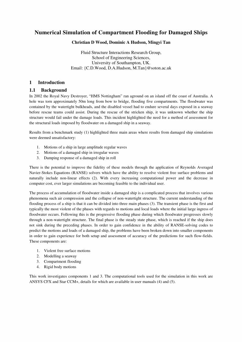
Numerical Simulation of Compartment Flooding for Damaged Ships

Christian D Wood, Dominic A Hudson, Mingyi Tan

Fluid Structure Interactions Research Group,

School of Engineering Sciences,

University of Southampton, UK.

Email: C.D.Wood, D.A.Hudson, M.Tan@soton.ac.uk

1 Introduction

1.1 Background

In 2002 the Royal Navy Destroyer, “HMS Nottingham” ran aground on an island off the coast of Australia. A

hole was torn approximately 50m long from bow to bridge, flooding five compartments. The floodwater was

contained by the watertight bulkheads, and the disabled vessel had to endure several days exposed in a seaway

before rescue teams could assist. During the rescue of the stricken ship, it was unknown whether the ship

structure would fail under the damage loads. This incident highlighted the need for a method of assessment for

the structural loads imposed by floodwater on a damaged ship in a seaway.

Results from a benchmark study (1) highlighted three main areas where results from damaged ship simulations

were deemed unsatisfactory:

1. Motions of a ship in large amplitude regular waves

2. Motions of a damaged ship in irregular waves

3. Damping response of a damaged ship in roll

There is the potential to improve the fidelity of these models through the application of Reynolds Averaged

Navier-Stokes Equations (RANSE) solvers which have the ability to resolve violent free surface problems and

naturally include non-linear effects (2). With every increasing computational power and the decrease in

computer cost, ever larger simulations are becoming feasible to the individual user.

The process of accumulation of floodwater inside a damaged ship is a complicated process that involves various

phenomena such air compression and the collapse of non-watertight structure. The current understanding of the

flooding process of a ship is that it can be divided into three main phases (3). The transient phase is the first and

typically the most violent of the phases with regards to motions and local loads where the initial large ingress of

floodwater occurs. Following this is the progressive flooding phase during which floodwater progresses slowly

through a non-watertight structure. The final phase is the steady state phase, which is reached if the ship does

not sink during the preceding phases. In order to gain confidence in the ability of RANSE-solving codes to

predict the motions and loads of a damaged ship, the problems have been broken down into smaller components

in order to gain experience for both setup and assessment of accuracy of the predictions for such flow-fields.

These components are:

1. Violent free surface motions

2. Modelling a seaway

3. Compartment flooding

4. Rigid body motions

This work investigates components 1 and 3. The computational tools used for the simulation in this work are

ANSYS CFX and Star CCM+, details for which are available in user manuals (4) and (5).

2 Dam-break

2.1 Domain

A diagram of the two dimensional problem is shown (6). The compartment size from the experimental

comparison is 3.22m long and 2.0m high with a column of water of 1.2m long and 0.6m high located at the

bottom left hand corner. There is a pressure sensor located on the right wall 0.16m from the bottom (for the

experimental set up the dimensions of the pressure sensor were a 90mm circle centered at the co-ordinates

shown on the diagram). The time period of interest takes place over the first 2.5 s.

Figure 1 - Domain setup (left), CFX grid (middle) and Star CCM+ grid (right)

Three separate hexahedral meshes were generated each for both Star CCM+ and ANSYS CFX for a grid

dependency study. The hexahedral meshes in Star CCM+ were generated within Star CCM+ and are

anisotropic; hence there is greater control over local refinement. This feature was used to reduce computational

time. The hexahedral meshes used in ANSYS were generated in ICEM and as with all 2D problems within CFX

are pseudo 2D (i.e. One cell thick in the third dimension).

Table 1 - Table of Meshes used for dambreak case

Mesh Cells Grid Setup

Hex Coarse 8422 25mm x 25mm Coarsened mesh outside of y<0.6m and x>2m

Hex Med 23312 15mm x 15mm and Coarse mesh outside of y<0.6m and x>2m Star

Hex Fine 52346 10mm x 10mm and Coarse mesh outside of y<0.6m and x>2m

Hex Coarse 7169 Uniform 30mm x 30mm

Hex Med 28676 Uniform 15mm x 15mm CFX

Hex Fine 64521 Uniform 10mm x 10mm

Boundary conditions for this case are simple as the majority are defined as no-slip walls. The top boundaries are

treated slightly differently within the two codes. In ANSYS CFX the treatment is by the use of an “opening”

boundary condition where the static pressure is entrained to 0 Pa. In Star CCM+ the boundary is defined as a

“pressure outlet” which stills allows fluid to enter and exit the domain much like the “opening” boundary

condition. For this condition static pressure is again set at 0Pa and a volume fraction of 0 is defined. The pseudo

2D nature of the ANSYS mesh requires that front and back boundary conditions are symmetry boundaries.

2.2 Simulation

Both cases are defined as Eulerian multiphase; the two phases are air and water. Libraries of material properties

are available in both packages for which material properties vary slightly. For both applications these were both

set at ρw=998.2 kgm-3

and ρa=1.225 kgm-3

. Atmospheric pressure for both simulations were set to 101325 Pa.

Gravity prescribed in the vertical direction at -9.81 ms-2

. For both solvers the k-ε turbulence model was used; in

CFX this was in conjunction with a wall function (4), in CCM+ a two layer approach is applied as described in

(5).

Initialisation of the domain was scripted using expression language in ANSYS CFX and the equivalent user

field functions in Star CCM+ to define volume fraction and hydrostatic pressure in the 2D domain.

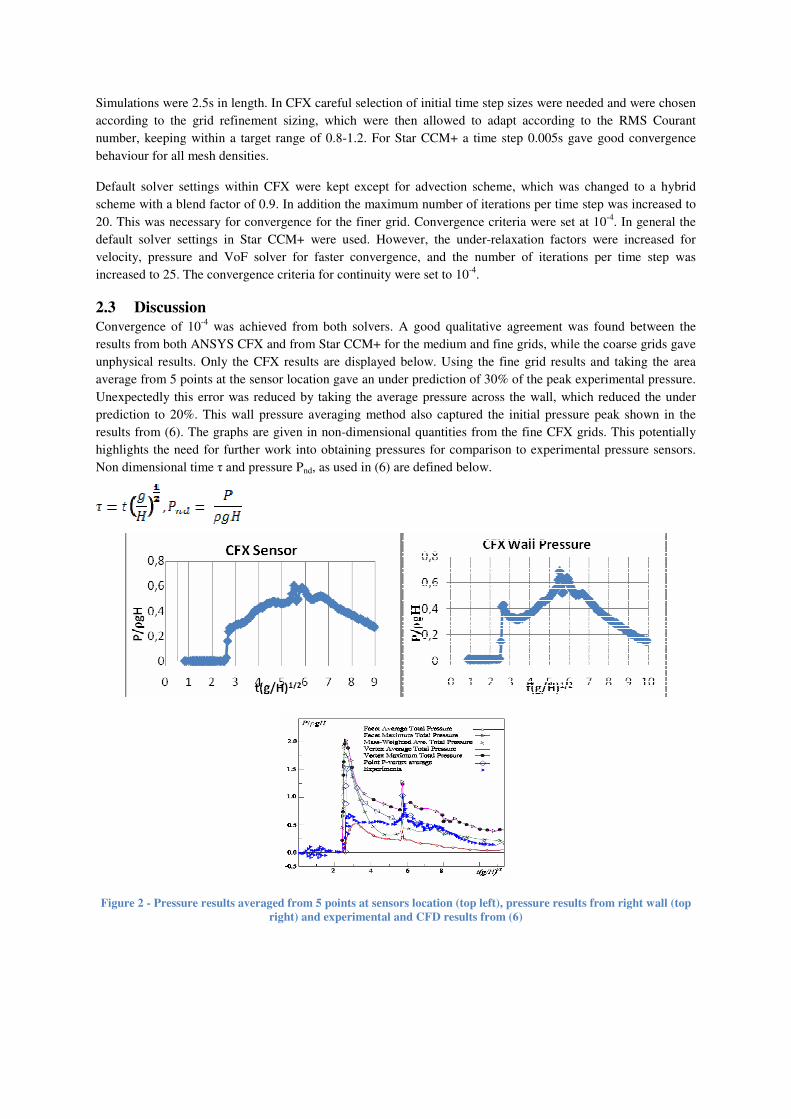
Simulations were 2.5s in length. In CFX careful selection of initial time step sizes were needed and were chosen

according to the grid refinement sizing, which were then allowed to adapt according to the RMS Courant

number, keeping within a target range of 0.8-1.2. For Star CCM+ a time step 0.005s gave good convergence

behaviour for all mesh densities.

Default solver settings within CFX were kept except for advection scheme, which was changed to a hybrid

scheme with a blend factor of 0.9. In addition the maximum number of iterations per time step was increased to

20. This was necessary for convergence for the finer grid. Convergence criteria were set at 10-4

. In general the

default solver settings in Star CCM+ were used. However, the under-relaxation factors were increased for

velocity, pressure and VoF solver for faster convergence, and the number of iterations per time step was

increased to 25. The convergence criteria for continuity were set to 10-4

.

2.3 Discussion

Convergence of 10-4

was achieved from both solvers. A good qualitative agreement was found between the

results from both ANSYS CFX and from Star CCM+ for the medium and fine grids, while the coarse grids gave

unphysical results. Only the CFX results are displayed below. Using the fine grid results and taking the area

average from 5 points at the sensor location gave an under prediction of 30% of the peak experimental pressure.

Unexpectedly this error was reduced by taking the average pressure across the wall, which reduced the under

prediction to 20%. This wall pressure averaging method also captured the initial pressure peak shown in the

results from (6). The graphs are given in non-dimensional quantities from the fine CFX grids. This potentially

highlights the need for further work into obtaining pressures for comparison to experimental pressure sensors.

Non dimensional time τ and pressure Pnd, as used in (6) are defined below.

Figure 2 - Pressure results averaged from 5 points at sensors location (top left), pressure results from right wall (top

right) and experimental and CFD results from (6)

3 Compartment Flooding

3.1 Domain

The tank flooding simulation is a 2D problem potentially comparable to some cases of grounding damage on a

ship. Outside of the compartment the water level is 0.75m high, whilst inside the compartment the water is at

0.5m. A small hole 0.02m wide is present in the hull section at the bottom.

Figure 3 - Domain setup (left), CFX grid (middle) and Star CCM+ grid (right)

3.2 Boundary Conditions

No-slip wall conditions were defined for the hull surfaces, left, right and bottom boundaries. The remaining

boundaries (the three surfaces above the water; one inside the hull and one either side) were modelled as

openings (CFX) or as stagnation inlets on the outside and pressure outlets on the inside (Star CCM+). All of

these boundary conditions were defined in such a way that the pressure at the boundary was to be entrained to

zero. Again with CFX, as the mesh is pseudo 2D, the front and back boundaries were symmetry boundaries.

3.3 Simulation

A Eulerian multiphase model is used where the two phases are air and water. Libraries of material properties are

available in both packages for which numbers vary slightly and again were both set at ρw=998.2 kgm-3

and

ρa=1.225 kgm-3

. Atmospheric pressure for both simulations were set to 101325 Pa and gravity prescribed in the

vertical direction at -9.81 ms-2

. During the grid dependency the k-ε turbulence model was used; in CFX this was

in conjunction with a wall function (4), whereas Star CCM+ a shear driven two layer approach is applied as

described in (5). Other turbulence models were tested for comparison.

Initialisation of the domain was done using expression language in ANSYS CFX and the equivalent user field

functions in Star CCM+ to define volume fraction and hydrostatic pressure in the 2D domain.

The majority of the settings used for dam-break were used for the compartment filling, the exceptions were;

simulation time is increased to 5 s and careful attention was given to the convergence levels in Star CCM+. The

importance of this is demonstrated in Figure 4. Inadequate convergence resulted in an non-symmetric jet

forming.

Figure 4 - Snapshots during first time step by continuity convergence level, from left to right; 2x10-2, 3x10-2, 8x10-3,

2x10-3, 7x10-4 and 2x10-4.

3.4 Discussion

Grid convergence was achieved on the three separate grids and three turbulence models were assessed against

each other on the coarse grid. The turbulence model survey was conducted using the coarse mesh to reduce

time, this could be improved by conducting it on the grid converged simulations in order to assess the impact of

turbulence model selection. Simulations using the coarse mesh flooded far more rapidly than the medium and

fine mesh. Coarse mesh simulations reached the equilibrium water level of 0.71m in approximately 2s, whereas

for the medium and fine meshes results were 3.5 s and 3.7 s respectively. It is expected that further mesh

refinements will give change as the level of fidelity increases and smaller turbulence scales are modelled which

affect the overall flow-field. Grid dependency and turbulence model survey results from CFX are shown in

Figure 5.

Figure 5 - Stages of Vena Contracta development in Star CCM+, 0.08s (left), 0.16s (middle) and grid dependency

study with turbulence model survey from CFX (right)

The contraction in the flow can be seen downstream of the orifice giving the classical vena contracta with

regions of circulation either side. These are shown using streamlines and the free surface.

Figure 6 - Time history of flooding from medium grid with free surface snapshots in CFX

The industry standard model of this case is derived from a special application of Bernoulli’s equation, but

modified to allow for the effects of the geometry with the use of a discharge co-efficient. In this form, it is

known as Toricelli’s formula.

Where Cd is the discharge co-efficient, A0 is the area of the hole, g is gravitational acceleration and h is the

height difference between the internal and external water levels. Instantaneous velocity at the orifice can be

taken from the RANS model and a discharge co-efficient can be calculated. The average velocity through the

orifice during the first 0.1s of the simulation was 1.31 ms-1

. Applying Bernoulli would give an instantaneous

orifice velocity of 2.21 ms-1

, giving a discharge co-efficient of 0.59. The results demonstrate that in this

particular scenario, Torricelli’s formula would substitute as an adequate model for ingress of water. However

this would remove any non-linear dynamic effects due to ship motion and wave effects inherent in the damaged

ship scenario. So the applicability of such a method in the author’s future work would be limited.

4 Conclusions

The results from the dam-break simulation show that CFD can give good qualitative results compared to

experimental data. It is the author’s belief that further refinement of the meshes could indeed give good

quantitative results, however this would be at a higher computational expense.

The results from the compartment flooding show the ingress of floodwater can be particularly violent,

particularly in the transient region of flooding. The fine mesh showed better convergence behavior with an in-

homogenous scheme, indicating that the flow becomes more complex with finer grid detail, although this slows

down the solution time significantly. Within this region it is believed Torricelli’s formula would be inadequate

in modeling the ingress of floodwater into a compartment. Further down the flooding process, during

progressive and steady state regions, Torricelli’s formula could potentially be adequate, however this is an area

of further work. In addition to this, the location of the damage and the presence of a wave field will also affect

the flow rates of floodwater, to a level that needs to be ascertained.

As a whole, it has been shown that CFD can model these non-linear effects, to a level that would be beneficial in

damaged ship simulation.

5 References

1. ITTC. Stability in Waves. Edinburgh, UK : s.n., 2005.

2. Computation of flow-induced motion of floating bodies. Hadzic, I, et al. 2005, Applied Mathematical

Modelling, Vol. 29, pp. 1196-1210.

3. Validation of a Simulation Method for Progressive Flooding. Ruponen, P, Sundell, T and Larmela, M. Rio

de Janeiro : s.n., 2006. Proceedings of the 9th International Conference on Stability of Ships and Ocean

Vehicles. pp. 607-616.

4. ANSYS. ANSYS CFX, Release 11.0 Help. 2007.

5. CD-Adapco. Star CCM+ v3.06.006 Help. 2008.

6. Simulation of the Dam Break Problem and Impact Flows Using a Navier-Stokes Solver. Abdolmaleki, K,

Thiagarajan, K P and Morris-Thomas, M T. Sydney : s.n., 2004. Proceedings of the 15th Austrlasian Fluid

Mechanics Conference.

Progress in Seaway-Simulations in Compact DomainsKatja Wockner, Withold Drazyk and Thomas Rung

katja.woeckner@tu-harburg.de

Hamburg University of Technology (TUHH), GermanyInstitute of Fluid Dynamics and Ship Theory (M-8)

Introduction

In conjunction with recent damages, an enhanced interest into the hydrodynamic performance of vessels ex-posed to hazardous operating conditions in waves is seen. Such situations might refer to manouvring abilitiesunder severe sea state. RANS-simulations of ships in seaways often employ the rigid-grid movement approachcombined with a volume-of-fluid (VOF) method to capture the position of the free surface. As opposed togrid-distortion techniques, the approach facilitates arbitrary ship motions.Unsteady RANS are however afflicted with high computational expenses due to the associated grid requirementsfor an accurate propagation of incident waves towards the ship and the Courant-number based time-step restric-tions. Accordingly, small computational domains are desirable to reduce the computational effort. Moreover,wave reflections from the far-field boundaries are difficult to manage. The latter is often adressed by means of agrid-stretching (”beach”) towards the outlet, which introduces a numerical damping zone. The approach aimsto completely dampen the wave field until the outlet boundary. Due to their inherent directionality, such gridsare not suitable for simulations of variable wave directions. A case in point refers to turning tests in waves,where the wave direction is earth-fixed, while the domain is moving and waves shall enter and leave the domainin all directions.Coupled potential flow/RANS methods are an attractive way out of the above mentioned dilemma. An appeal-ing one-way coupling between an inviscid baseline solution and a subsequent viscous solver, named Spectral-Wave-Energy Navier-Stokes-Equations (SWENSE), has been devised by researchers from ECN [4] for interfacetracking methods. The paper reports the application of an alternative approach [2] for the solver FreSCo [3],which uses a VOF method to capture the free surface.

Mathematical Model

In view of an efficient approach, a (one-way) coupling of an inviscid method to a RANS procedure is viable.To eliminate any interface problems, the respective coupling should be non-zonal. The SWENSE approach [4]focuses on interface tracking methods and separates an explicitly known baseline solution for the propagationfield (φProp) from the Navier-Stokes solution:

φNS = φProp + φ.

Appropriate governing equations are derived from the Navier-Stokes equation for the supplement φ. Essentially,the Navier-Stokes equation is solved for the unknown supplement φ instead of the actual variable φNS . Thebenefit occurs in conjunction with the formulation of the far-field boundary condition, which refers to a vanishingsupplement and thus promotes the adherence to the far-field propagation solution in a natural way. In orderto account for severe sea-states, involving breaking waves, the RANS method should be based on an interface-capturing technique.The present work is not based upon a formal decomposition of the flow into a diffracted and a baseline field.The suggestion aims to establish an implicit coupling using dirichlet far-field conditions and a manipulationof the coefficient matrix over a far-field buffer-zone to apply the inviscid background-solution. In terms of thefar-field boundary condition, the approach is quite similar to the SWENSE. However, since the diffracted fieldis not explicitly computed in the present suggestion, the damping of the diffraction waves has to be managedthrough an appropriate construction of the buffer-zone parameters.An example for a computational domain and the used boundary conditions is shown in figure 1. Identicaldirichlet conditions for the velocities and the volume fraction are employed along the vertical boundaries. Todistinguish between different situations, we call a boundary ”wave-inlet”, if waves enter the domain and ”wave-outlet” if waves leave the domain. Mind, that the horizontal planes (indicated by ”neumann”) are assigned todirichlet conditions for the pressure and neumann conditions for the velocity and the volume fraction.The Airy theory [1] is used to calculate the potential flow solution. Accordingly, the elevation ζ of the freesurface follows from

ζ = ζSW + ζcos(ωt − kx) . (1)

1

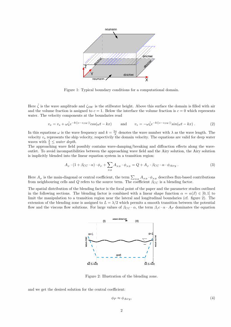
Figure 1: Typical boundary conditions for a computational domain.

Here ζ is the wave amplitude and ζSW is the stillwater height. Above this surface the domain is filled with airand the volume fraction is assigned to c = 1. Below the interface the volume fraction is c = 0 which representswater. The velocity components at the boundaries read

vx = vs + ωζe−k(|z−zSW |)cos(ωt − kx) and vz = −ωζe−k(|z−zSW |)sin(ωt − kx) . (2)

In this equations ω is the wave frequency and k = 2πλ denotes the wave number with λ as the wave length. The

velocity vs represents the ship velocity, respectivily the domain velocity. The equations are valid for deep waterwaves with λ

2 ≤ water depth.The approaching wave field possibly contains wave-damping/breaking and diffraction effects along the wave-outlet. To avoid incompatibilities between the approaching wave field and the Airy solution, the Airy solutionis implicitly blended into the linear equation system in a transition region:

AP · (1 + βCC · α) · φP +∑NB

ANB · φNB = Q + AP · βCC · α · φAiry . (3)

Here AP

is the main-diagonal or central coefficient, the term∑

NBA

NB·φ

NBdescribes flux-based contributions

from neighbouring cells and Q refers to the source term. The coefficient βCC is a blending factor.

The spatial distribution of the blending factor is the focal point of the paper and the parameter studies outlinedin the following sections. The blending factor is combined with a linear shape function α = α(~x) ∈ [0, 1] tolimit the manipulation to a transition region near the lateral and longitudinal boundaries (cf. figure 2). Theextension of the blending zone is assigned to L = λ/2 which permits a smooth transition between the potentialflow and the viscous flow solutions. For large values of βCC · α, the term βcc · α · AP dominates the equation

Figure 2: Illustration of the blending zone.

and we get the desired solution for the central coefficient:

φP ≈ φAiry, (4)

2

which means that the calculated solution is equal to the Airy wave. For the momentum equations φAiry

represents the orbital velocities of the waves calculated with equation 2, while the distribution of the volumefraction is calculated according to equation 1. The aim of this modifikation is to have a smooth transitionbetween the undisturbed potential waves at the boundaries and the viscous waves inside the domain. Withoutthis transformation, which forces a prescibed wave pattern, reflections would occur at the outlet boundaries.The difficulty in this approach is to determine the coefficient βCC , because too small values for βCC lead towave reflections at the actual wave-outlet (right border in figure 2), while in case of too large values, wavereflections occur at the transition point (marked with (II) in figure 2) between the modified region (α 6= 0) andthe un-modified region (α = 0).

Two-Dimensional Wave Tank

A simple 2D wave tank without any obstacle is investigated as a first testcase. The domain and the usedboundary conditions can be taken from figure 3. Boundary regions marked with “wave” refer to dirichletconditions for the volume fraction and the velocities. The respective boundary values are obtained from theAiry theory (see eq. 1 and 2). The keyword “pressure” at the top and bottom of the domain indicates the useof hydrostatic pressure values.

Figure 3: Physical domain and numerical grid for the 2D wave tank testcase.

The example refers to waves travelling from left to right. We monitor the height of the free surface at differentlocations inside the domain to assess the influence of the manipulations. Figure 4 displays exemplary results ofthe computational exercise for λ = 5m, ζ = 0.1m and vs = −1m

s .

The figure shows the computed free-surface elevation normalised with the respective elevation obtained from theAiry theory (1) at discrete locations (marked with circles). The filled circles outline the borders of the blendingzones. The three graphs in figure 4 show calculations with different blending factors (βCC = (0.01; 0.05; 0.25)).In the upper left graph the amplitudes do not reach the full height at the actual wave-outlet. Due to a too smallvalue for βCC a transformation of the calculated wave into the Airy wave is not possible within the blendingzone. The upper right picture shows a sudden change in the height of the amplitudes at the begin of theblending zone, which is a result of a too large value for βCC , while the third picture shows a smooth transitionbetween the calculated waves in the middle of the domain and the waves at the boundary. This indicates thata transformation into the Airy wave is possible without any reflections of waves.

Three-dimensional Wave Tank with Obstacle

The second testcase refers to a 3D wave tank with a fixed cuboid in the centre of the domain, as shown in figure5. The investigated uni-directional wave field is confined to λ = 5m, ζ = 0.1m, vs = −1m

s and the blendingfactor is varied between βCC = (0; 0.05; 0.1; 1). The cuboid has a large influence on the wave field. Since thedomain is small compared to the wave length, the differences between the Airy wave and the calculated wavefield are expected to be more pronounced. The case is challenging because large manipulations are imposed onthe flow field while the waves pass the blending zone. It should reveal the error in case a full recovery of thewave in the blending zone is not possible.Results of the predicted drag force coefficient are shown in figure 6. The forces are compared to results obtainedin conjunction with a numerical beach. Calculations based upon βCC 6= 0 return larger maxima and smallerminima than computations with a numerical beach, which are a result of wave reflections at the begin of the

3

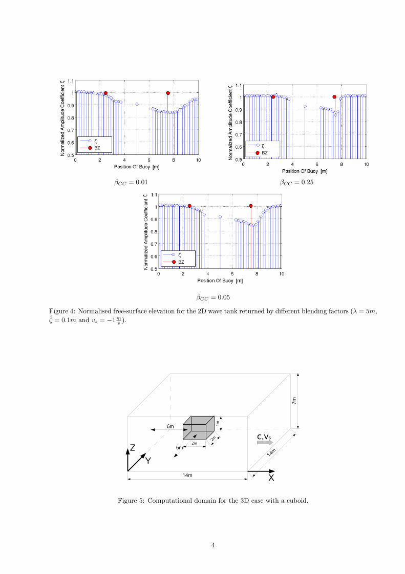
βCC = 0.01 βCC = 0.25

βCC = 0.05

Figure 4: Normalised free-surface elevation for the 2D wave tank returned by different blending factors (λ = 5m,ζ = 0.1m and vs = −1m

s ).

Figure 5: Computational domain for the 3D case with a cuboid.

4

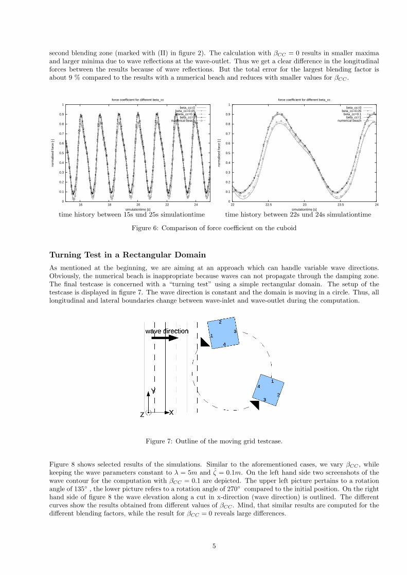
second blending zone (marked with (II) in figure 2). The calculation with βCC = 0 results in smaller maximaand larger minima due to wave reflections at the wave-outlet. Thus we get a clear difference in the longitudinalforces between the results because of wave reflections. But the total error for the largest blending factor isabout 9 % compared to the results with a numerical beach and reduces with smaller values for βCC .

0

0.1

0.2

0.3

0.4

0.5

0.6

0.7

0.8

0.9

1

16 18 20 22 24

norm

alis

ed fo

rce

[-]

simulationtime [s]

force coefficient for different beta_cc

beta_cc=0beta_cc=0.05beta_cc=0.1

beta_cc=1numerical beach

time history between 15s und 25s simulationtime

0

0.1

0.2

0.3

0.4

0.5

0.6

0.7

0.8

0.9

1

22 22.5 23 23.5 24

norm

alis

ed fo

rce

[-]

simulationtime [s]

force coefficient for different beta_cc

beta_cc=0beta_cc=0.05beta_cc=0.1

beta_cc=1numerical beach

time history between 22s und 24s simulationtime

Figure 6: Comparison of force coefficient on the cuboid

Turning Test in a Rectangular Domain

As mentioned at the beginning, we are aiming at an approach which can handle variable wave directions.Obviously, the numerical beach is inappropriate because waves can not propagate through the damping zone.The final testcase is concerned with a “turning test” using a simple rectangular domain. The setup of thetestcase is displayed in figure 7. The wave direction is constant and the domain is moving in a circle. Thus, alllongitudinal and lateral boundaries change between wave-inlet and wave-outlet during the computation.

Figure 7: Outline of the moving grid testcase.

Figure 8 shows selected results of the simulations. Similar to the aforementioned cases, we vary βCC , whilekeeping the wave parameters constant to λ = 5m and ζ = 0.1m. On the left hand side two screenshots of thewave contour for the computation with βCC = 0.1 are depicted. The upper left picture pertains to a rotationangle of 135 , the lower picture refers to a rotation angle of 270 compared to the initial position. On the righthand side of figure 8 the wave elevation along a cut in x-direction (wave direction) is outlined. The differentcurves show the results obtained from different values of βCC . Mind, that similar results are computed for thedifferent blending factors, while the result for βCC = 0 reveals large differences.

5

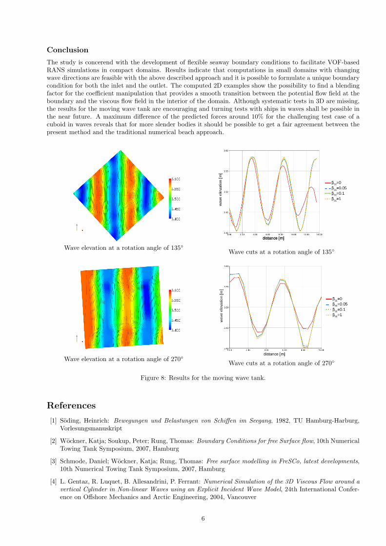
Conclusion

The study is concerend with the development of flexible seaway boundary conditions to facilitate VOF-basedRANS simulations in compact domains. Results indicate that computations in small domains with changingwave directions are feasible with the above described approach and it is possible to formulate a unique boundarycondition for both the inlet and the outlet. The computed 2D examples show the possibility to find a blendingfactor for the coefficient manipulation that provides a smooth transition between the potential flow field at theboundary and the viscous flow field in the interior of the domain. Although systematic tests in 3D are missing,the results for the moving wave tank are encouraging and turning tests with ships in waves shall be possible inthe near future. A maximum difference of the predicted forces around 10% for the challenging test case of acuboid in waves reveals that for more slender bodies it should be possible to get a fair agreement between thepresent method and the traditional numerical beach approach.

Wave elevation at a rotation angle of 135Wave cuts at a rotation angle of 135

Wave elevation at a rotation angle of 270Wave cuts at a rotation angle of 270

Figure 8: Results for the moving wave tank.

References

[1] Soding, Heinrich: Bewegungen und Belastungen von Schiffen im Seegang, 1982, TU Hamburg-Harburg,Vorlesungsmanuskript

[2] Wockner, Katja; Soukup, Peter; Rung, Thomas: Boundary Conditions for free Surface flow, 10th NumericalTowing Tank Symposium, 2007, Hamburg

[3] Schmode, Daniel; Wockner, Katja; Rung, Thomas: Free surface modelling in FreSCo, latest developments,10th Numerical Towing Tank Symposium, 2007, Hamburg

[4] L. Gentaz, R. Luquet, B. Allesandrini, P. Ferrant: Numerical Simulation of the 3D Viscous Flow around avertical Cylinder in Non-linear Waves using an Explicit Incident Wave Model, 24th International Confer-ence on Offshore Mechanics and Arctic Engineering, 2004, Vancouver

6

CALL FOR PAPERS

13th

Numerical Towing Tank Symposium (NuTTS'10)

Duisburg, Germany, 10.-12.10.2010

Topics:

- Nonlinear flows around marine structures (LES, RANSE, Euler with or w/o free surface)

- Free-surface flows around marine structures (3-d ship seakeeping, free-surface viscous flows)

- Related topics (validation experiments, numerical techniques, grid generation, etc)

Deadlines: Early feedback (optional): 30 April 2010

Extended Abstracts received: 30 July 2010

Payment received: 30 August 2010

You are invited to participate in the above event. The objective of the event is to provide a forum for

informal discussions among experts in the field and to disseminate latest results. Younger workers and Ph.D.

students are especially encouraged to participate. The event will be held at “Die Wolfsburg” in Duisburg.

All participants stay and have meals together to maximize interaction and discussion.

The extended abstracts of the proposed talk will be directly reproduced in pdf proceedings. Work in

progress, encountered problems, etc. should be discussed in an open, informal atmosphere (no ties!) among

colleagues. The first page of the extended abstract should be headed with the title and authors' names,

affiliation and email address in a compact form to economize on space. Academic titles and page numbers

shall be omitted. The extended abstract shall neither contain an abstract of the abstract, nor keywords, nor

further headers. Font size shall not be less than 10pt Times New Roman. Extended abstracts should be

limited to 6 pages in A4 format with 2.5 cm margin. An early reply will help us in organizing the event

better. For the early feedback, a tentative title or topic will suffice.

Following the tradition of previous NuTTS events, the fees will be kept low to allow a maximum number of

scientists to attend. The fees including accommodation (3 nights) and meals during the symposium will be:

250 Euro PhD candidates and students

300 Euro authors (in single room)

350 Euro other participants (in single room)

Contact: Prof. Dr.Ing. Ould El Moctar, dagmar.elsner-kettenis@uni-due.de

Sponsors: To be announced