1

Stereo PIV flow-calibration in towing tank

S. Grizzi, F. di Felice

INSEAN, Italian model ship basin, via di vallerano 139, 00129 Rome, Italy

Abstract An enhancement of Stereo PIV calibration is

presented. The feature of this technique is to

calibrate the Stereo system directly from a

uniform flow measurement. This is achieved

making a first two-dimensional calibration

of the measurement plane using a standard

dotted target, then getting information of

perspective and laser sheet thickness from

some measurements of well-known flows

(uniform flow). This technique results in

three-dimensional measurements of high

accuracy with a simple calibration phase and

reduces mechanical misalignment and dot

recognition errors.

A very simple application of this technique

is performed in towing tanks. The technique

is tested to a tip vortex couple of a

submarine bridge fin.

Introduction Stereo particle image velocimetry (SPIV) is

an extension of traditional particle image

velocimetry (PIV) (Arroyo and Greated

1991; Willert 1997; Prasad 2000).

Using principles of stereoscopic vision,

SPIV reconstructs the three-component

velocity field in a two-dimensional plane

using two velocity fields derived using PIV

from two cameras.

This reconstruction process uses geometrical

equations, calibrated to consider geometrical

information of the stereoscopic system, to

link the image planes to events occurring in

the object plane.

Different calibration techniques are possible:

Geometric reconstruction relates the

parameters of image acquisition and the

measured two-dimensional velocity fields

through geometrical parameters of the

stereoscopic system (Prasad and Adrian

1993). Those parameters are affected by

measurement uncertain and for complex

stereoscopic configurations became more

difficult.

Two-dimensional calibration uses

geometrical parameters to perform the

reconstruction, similar to geometric

reconstruction. It differs because the

distortion field is derived from the

calibration process rather than calculating

distortion directly from the geometric

parameters.

Three-dimensional calibration techniques

are more commonly used than two-

dimensional ones (Soloff et al. 1997).

The main advantage of three-dimensional

calibration is that geometric information of

the stereoscopic system is not required.

Mapping functions are calibrated using a

number of parallel planes near the imaging

plane. In this way the functions correct

distortions and contain also geometrical

information required in reconstruction

phase.

The three-dimensional calibration technique

uses a calibration target, which consists of a

regular Cartesian grid of markers (Lawson

and Wu 1997).

Unfortunately the calibration phase is

affected by misalignment errors of the

calibration target and the laser sheet and

shifting errors when target is moved on

parallel planes near the imaging one.

An interesting idea was developed in Willert

(1997) and further in Wieneke (2005). This

idea is to use the cross correlation of the

particle images to generate additional

information (disparity maps) for correcting

the misalignment errors but this adds

complexity and increase computational cost.

Aim of present work is to introduce a simple

calibration method based on a standard two-

dimensional calibration for linking object

plane with camera planes adding three-

dimensional information obtained by a

uniform flow.

2

Flow Calibration Usually in a Soloff based algorithm the

calibration phase is accomplished by the

definition of polynomial mapping functions

between object and camera planes.

This type of calibration defines polynomial

coefficients using least-square applied on a

three-dimensional group of points extracted

from many target positions.

Calibration points are extracted by many

images of a dotted target placed on parallel

planes around center of the laser sheet.

In this phase misalignment errors between

laser sheet and target plane are possible and

are also possible mechanical misalignments

during shifting of it.

The presented technique instead uses only

two-dimensional information from a target

image to define correspondence between

cameras and object plane and obtain

additional necessary information from

acquisitions of a constant flow field. In fact

the knowledge of a constant flow

(W0(x,y,z,t) = C) projected on both camera

planes contain information about distortions,

optical aberrations and misalignment errors,

moreover this calibration is not affected by

target shifting errors.

Calibrating mapping functions using this

information gives the capability to

reconstruct 2D3C flow and at the same time

to correct misalignment errors.

Necessary to this phase is to have an exactly

constant flow, for this reason this technique

is easy in towing tanks, in fact having a

stagnant water tank and mounting the stereo

system on a carriage is possible to move it in

water to a constant speed obtaining so

desired fields.

Assuming z = 0 plane the center of the laser

sheet, the reference acquisition is made to a

constant speed W0 with a delay time Dt

between two consecutive frames, so is

reasonable to assume that frames gives a

better description of the laser volume

between z = -W0*Dt/2 and z = +W0*Dt/2

zone. Changing W0 speed or delay time Dt is

possible to obtain a more complete

description of laser sheet thickness until

correlation fails, which indicates particles

trespassing laser sheet.

Polynomial mapping functions are used

(Soloff et al. 1997) (Eq.1). In a first step the

degree of the polynomial is 2nd

for x and y

and is 1st for z.

(X,Y)l,r = ∑ ai*xj*y

k*z

m Eq.1

In these functions, absolute object

coordinates (x,y,z) and cameras coordinates

(X,Y)l,r are present.

A coordinate change is necessary to

introduce velocity information from constant

field, in fact x= x0+Dx and Dx=U*Dt. The

x0, y0 and z0 information are given by two-

dimensional calibration and U0, V0, W0 are

given by calibration flow acquisition.

The 2D3C field reconstruction uses mapping

functions gradients as follow:

xxFX

j

iji

x

FF

,)(

With i=1,2 and j=1,2,3

3

2

1

)2(

3,2

)2(

2,2

)2(

1,2

)2(

3,1

)2(

2,1

)2(

1,1

)1(

3,2

)1(

2,2

)1(

1,2

)1(

3,1

)1(

2,1

)1(

1,1

)2(

2

)2(

1

)1(

2

)1(

1

x

x

x

FFF

FFF

FFF

FFF

X

X

X

X

(Soloff et al. 1997)

To comparing results, Soloff based

algorithm with standard three-dimensional

calibration are used.

Experimental Setup The used Stereo PIV system is a fully

submersible probe (Pereira et al. 2003); it is

equipped with two 2048x2048 px2

CCD

cameras and a 200 mJ Nd-YAG laser. The

system is modular and can be assembled into

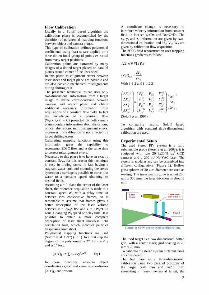
different configurations (Figure 1). Hollow

glass spheres of 30 mm diameter are used as

seeding. The investigation zone is about 250

mm x 300 mm, the laser thickness is about 5

mm.

Figure 1: SPIV probe used configuration.

The used target is a two-dimensional dotted

grid, with a center mark; grid spacing is 20

mm x 20 mm.

To calibrate the stereo system different cases

are considered.

The first case is a three-dimensional

calibration using two parallel positions of

the target (z=0 mm and z=2.5 mm)

simulating a three-dimensional target, the

3

degree of the mapping polynomial is the 2nd

for x and y and is the 1st for z.

The second case is a three-dimensional

calibration using thirteen parallel positions

of the target (2 mm spacing between each

position), the degree of the mapping

polynomial is the 3rd

for x and y and is the

2nd

for z.

The second case is a three-dimensional

calibration using thirteen parallel positions

of the target (2 mm spacing between each

position), the degree of the mapping

polynomial is the 4th

for x and y and is the

3rd

for z.

The fourth case is a two-dimensional

calibration using the z=0 position of the

target added to the constant flow calibration

with only 1 value of the displacement

±W0*Dt/2 (Flow Calibration), the degree of

the mapping polynomial is the 2nd

for x and

y and is the 1st for z.

The fifth case is a flow calibration using

mapping polynomial functions, 3rd

x and y

and 2nd

z degree.

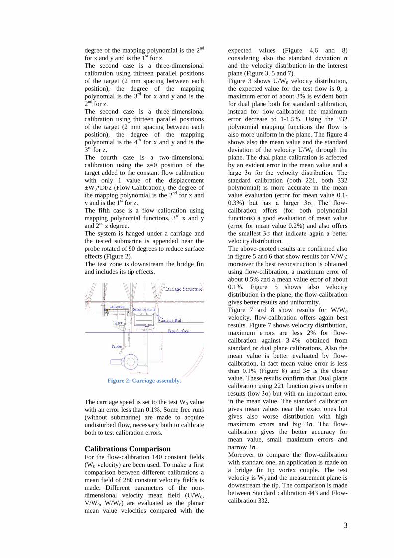
The system is hanged under a carriage and

the tested submarine is appended near the

probe rotated of 90 degrees to reduce surface

effects (Figure 2).

The test zone is downstream the bridge fin

and includes its tip effects.

Figure 2: Carriage assembly.

The carriage speed is set to the test W0 value

with an error less than 0.1%. Some free runs

(without submarine) are made to acquire

undisturbed flow, necessary both to calibrate

both to test calibration errors.

Calibrations Comparison For the flow-calibration 140 constant fields

(W0 velocity) are been used. To make a first

comparison between different calibrations a

mean field of 280 constant velocity fields is

made. Different parameters of the non-

dimensional velocity mean field (U/W0,

V/W0, W/W0) are evaluated as the planar

mean value velocities compared with the

expected values (Figure 4,6 and 8)

considering also the standard deviation σ

and the velocity distribution in the interest

plane (Figure 3, 5 and 7).

Figure 3 shows U/W0 velocity distribution,

the expected value for the test flow is 0, a

maximum error of about 3% is evident both

for dual plane both for standard calibration,

instead for flow-calibration the maximum

error decrease to 1-1.5%. Using the 332

polynomial mapping functions the flow is

also more uniform in the plane. The figure 4

shows also the mean value and the standard

deviation of the velocity U/W0 through the

plane. The dual plane calibration is affected

by an evident error in the mean value and a

large 3σ for the velocity distribution. The

standard calibration (both 221, both 332

polynomial) is more accurate in the mean

value evaluation (error for mean value 0.1-

0.3%) but has a larger 3σ. The flow-

calibration offers (for both polynomial

functions) a good evaluation of mean value

(error for mean value 0.2%) and also offers

the smallest 3σ that indicate again a better

velocity distribution.

The above-quoted results are confirmed also

in figure 5 and 6 that show results for V/W0;

moreover the best reconstruction is obtained

using flow-calibration, a maximum error of

about 0.5% and a mean value error of about

0.1%. Figure 5 shows also velocity

distribution in the plane, the flow-calibration

gives better results and uniformity.

Figure 7 and 8 show results for W/W0

velocity, flow-calibration offers again best

results. Figure 7 shows velocity distribution,

maximum errors are less 2% for flow-

calibration against 3-4% obtained from

standard or dual plane calibrations. Also the

mean value is better evaluated by flow-

calibration, in fact mean value error is less

than 0.1% (Figure 8) and 3σ is the closer

value. These results confirm that Dual plane

calibration using 221 function gives uniform

results (low 3σ) but with an important error

in the mean value. The standard calibration

gives mean values near the exact ones but

gives also worse distribution with high

maximum errors and big 3σ. The flow-

calibration gives the better accuracy for

mean value, small maximum errors and

narrow 3σ.

Moreover to compare the flow-calibration

with standard one, an application is made on

a bridge fin tip vortex couple. The test

velocity is W0 and the measurement plane is

downstream the tip. The comparison is made

between Standard calibration 443 and Flow-

calibration 332.

4

Figure 4: U/W0 planar mean value. Error bars indicate ±3σ.

Figure 3: U/W0 distribution.

5

Figure 6: V/W0 planar mean value. Error bars indicate ±3σ.

Figure 5: V/W0 distribution.

6

Figure 8: W/W0 planar mean value. Error bars indicate ±3σ.

Figure 7: W/W0 distribution.

7

Tip Vortex Couple A couple of tip vortexes are generated by the

bridge fin moving with a 0° drift angle from

the tip. The bridge fin can be assimilated to

a bold wing with a high thickness and low

aspect ratio, so the pressure distribution

forces the flow to move around the tip,

because the thickness of the fin and the 0°

drift angle, two opposite vortex are

generated (Figure 9).

Figure 9: Bridge fin: tip vortex couple.

Figure 10 shows the non-dimensional

velocity W/W0 for the interest plane

(Standard calibration 433 versus Flow

calibration 332) results are obtained using

175 acquired frames.

As expected the flow-calibration (332) gives

a more uniform external flow, less

influenced by optical aberrations and

misalignment errors, in fact this

reconstruction corrects this kind of errors.

Figure 10: Couple of tip vortexes W/W0

Figure 11 shows a detail of the vorticity and

cross flow: no differences are evident

principally for the vorticity field; this

indicates that the errors on the gradients are

negligible. To evaluate cross flow errors, a

comparison between velocities extracted on

the red line in Figure 11 is made (Figure 12

and 13).

Figure 11: Vorticity (up) and Cross Flow

(down): the red line is the comparison line.

As expected, there are relevant differences

principally regarding U/W0 velocity, all the

stereo reconstructions give good results for

V component but for U component the flow-

calibration based one gives less errors

especially in the peripheral zones of the

field.

8

Conclusions The flow-calibration method is a simple and

efficient algorithm for calibrating

Polynomial mapping functions, using a

constant flow no alignment errors are

present and optical aberrations are

accurately compensated.

Unfortunately to have an accurate uniform

flow a towing tank is needed.

The residual errors are generated principally

during the interpolation phase of the stereo

reconstruction. Future enhancements of this

stereo-technique are settled to correct also

numerical errors.

Acknowledgements The present work was supported by the

Italian “MINISTERO DEI TRASPORTI” in

the framework of the INSEAN “Programma

Ricerche Luglio 2006 – Dicembre 2007”.

Figure 12: U/W0 Comparison on the red line.

Figure 13: V/W0 Comparison on the red line.

9

References

Arroyo M, Greated C (1991) Stereoscopic particle image velocimetry. Meas Sci Technol 2:1181–1186

Lawson N, Wu J (1997) Three-dimensional particle image velocimetry: experimental error analysis of a

digital angular stereoscopic system. Meas Sci Technol

8:1455–1464

Pereira F, Costa T, Felli M, Calcagno G, Di Felice F (2003) A versatile fully submersible Stereo-PIV probe for tow tank applications. 4th ASME_JSME Joint

Fluids Engineering Conference, Honolulu, Hawaii,

USA

Prasad A, Adrian R (1993) Stereoscopic particle

image velocimetry applied to liquid flows. Exp Fluids 15:49–60

Prasad A (2000) Stereoscopic particle image velocimetry. Exp Fluids 29:103–116

Raffel M, Willert C, Kompenhans J (1998) Particle image velocimetry: a practical guide. Springer, Berlin

Soloff S, Adrian R, Liu Z (1997) Distortion compensation for generalized stereoscopic particle

image velocimetry. Meas Sci Technol 8:1441–1454

Wieneke B (2005) Stereo-piv using self-calibration on particle images. Exp Fluids 39:267–280

Willert C (1997) Stereoscopic digital particle image velocimetry for application in wind tunnel flows. Meas

Sci Technol 8:1465–1479

Zang W, Prasad A (1997) Performance evaluation of a

Scheimpflug stereocamera for particle image

velocimetry. Appl Opt 36:8738– 8744