1 Imaging Techniques for Flow and Motion Measurement Lecture 18 Lichuan Gui University of...
29
1 Imaging Techniques for Flow and Motion Measurement Lecture 18 Lichuan Gui University of Mississippi 2011 Large-scale PIV and Large-scale PIV and Stereo High-Speed Imaging Stereo High-Speed Imaging
-
Upload
iris-phillips -
Category
Documents
-
view
223 -
download
0
Transcript of 1 Imaging Techniques for Flow and Motion Measurement Lecture 18 Lichuan Gui University of...

1
Imaging Techniques for Flow and Motion Measurement
Lecture 18
Lichuan Gui
University of Mississippi
2011
Large-scale PIV and Large-scale PIV and
Stereo High-Speed ImagingStereo High-Speed Imaging

2
Large-Scale PIVLarge-Scale PIVRiver surface flow measurement
City map
river
Tower
Video set at 40m height
Camera view
Floating tracer

3
Large-Scale PIVLarge-Scale PIVRiver surface flow measurement
Original image
Calibrated image
Physical & image coordinates
Flow filed

4
Large-Scale PIVLarge-Scale PIVDistorted image calibration
Physical & image coordinates- Physical coordinates (X,Y)
- Image coordinates (x,y)
- Calibration marking points (Xk,Yk) (xk,yk) for k=1,2,,N
- Image calibration function
1,
1 54
876
54
321
ybxb
bybxbY
ybxb
bybxbX
Minimal N=4 for determining constants bi (i=1,2,,8)
- inverse calibration function
716242516574
6381143846
716242516574
8275532785
bbbbYbbbbXbbbb
bbbbYbbbXbbby
bbbbYbbbbXbbbb
bbbbYbbbXbbbx
Straight-line-conservedtransformation

5
Large-Scale PIVLarge-Scale PIVDistorted image calibration
4
3
2
1
4
3
2
1
8
7
6
5
4
3
2
1
444444
333333
222222
111111
444444
333333
222222
111111
1000
1000
1000
1000
0001
0001
0001
0001
Y
Y
Y
Y
X
X
X
X
b
b
b
b
b
b
b
b
yxYyYx
yxYyYx
yxYyYx
yxYyYx
XyXxyx
XyXxyx
XyXxyx
XyXxyx4 marking points
>4 marking points – least square approach
N
kkkkkkkkkkkkk YXbbybxbYXybYXxbbybx
1
287654321
8,,2,10
iforbi

6
Large-Scale PIVLarge-Scale PIVEvaluation of LSPIV recordings- Low-Image-Density PIV mode Particle image tracking or individual particle image pattern tracking
- Low Re-number in many cases Average correlation method for steady flows
Consecutive LSPIV recordings Evaluation results
Example of LSPIV tests for steady water surface flow

7
Large-Scale PIVLarge-Scale PIV
– References
• Muto Y, Baba Y, Aya S (2002) Velocity measurements in open channel flow with rectangular embayments formed by spur dykes. Annuals of Disas. Prev. Res. Inst., Kyoto Univ., No.45B-2
• Fujita I, Aya S, Deguchi T (1997) Surface velocity measurement of river flow using video images of an oblique angle. Proc. 27th IAHR Cong., San Francisco, Vol.B, No.1, pp.227-232
– Practice with EDPIV
• Work with sample: IMAGE GROUP: DISTORTED PIV IMAGES

8
Stereo High-Speed ImagingStereo High-Speed Imaging
Gray value resolution
10-bit CMOS sensor
17.5µm pixels
Frame rate & digital resolution
10241024 @ 2000 fps
1024256 @ 8000 fps
- High-speed camera

Stereo High-Speed ImagingStereo High-Speed Imaging- Optical configuration outside the
camera Mirror
Lens
Mirror
Alate
Mirrorimage
Mirror image
Front view
Side view
10
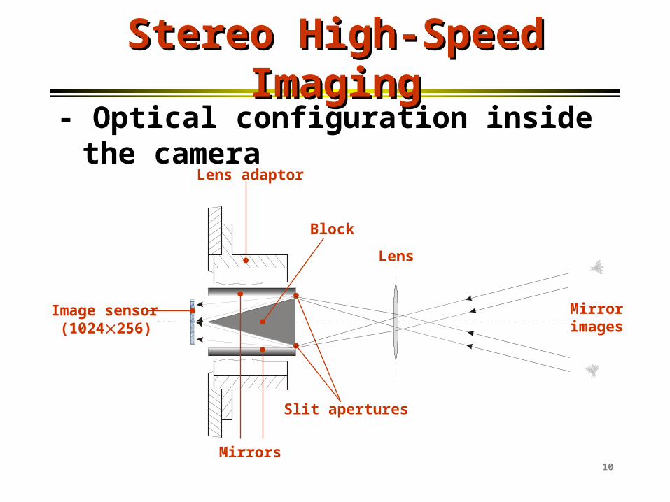
Stereo High-Speed ImagingStereo High-Speed Imaging
Lens adaptor
Mirrors
Image sensor (1024256)
Block
Slit apertures
Lens
Mirror images
- Optical configuration inside the camera

11
Stereo High-Speed ImagingStereo High-Speed Imaging
High-speed camera Mirrors Back lighting
Tethered fire ant alate Microphones
- Experimental setup with sound recording

12
Stereo High-Speed ImagingStereo High-Speed Imaging- Experimental setup with sound recording
Sound recorded from bottom & rear with MCDL

13
Stereo High-Speed ImagingStereo High-Speed Imaging- Sample image & postprocessing
Raw image
Background
Processed
14
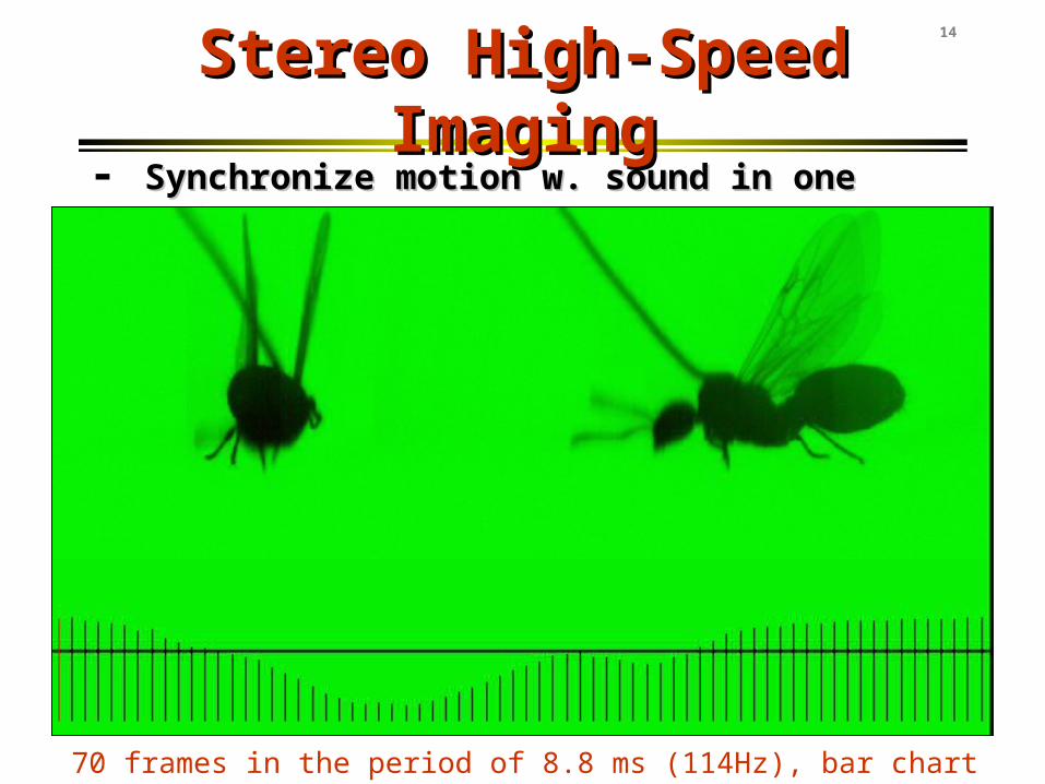
Stereo High-Speed ImagingStereo High-Speed Imaging
70 frames in the period of 8.8 ms (114Hz), bar chart represents sound pressure
- Synchronize motion w. sound in one period Synchronize motion w. sound in one period

15
Stereo High-Speed ImagingStereo High-Speed Imaging
- New optic table and magnetic holders for higher precision
- New template for adjusting mirror angles to ensure 90o difference between front and side- views
- Tested ant body carefully oriented
- Improved system for wing motion reconstruction

16
Stereo High-Speed ImagingStereo High-Speed Imaging
O: root of the wing T: tip of the wing 3: the 3rd point at the wing surface
- Position & orientation of the wing Position & orientation of the wing • the wing assumed to be a planar surface without thickness
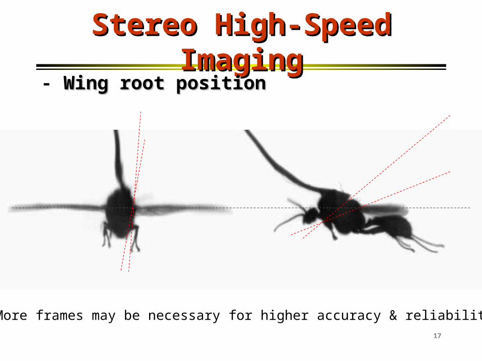
17
Stereo High-Speed ImagingStereo High-Speed Imaging- Wing root positionWing root position
More frames may be necessary for higher accuracy & reliability

18
Stereo High-Speed ImagingStereo High-Speed Imaging- 3D view of the wing surface D view of the wing surface
: angle between wing surface & plane through OT & OZ
xy: wing angle in xy-plane
zy: wing angle in yz-plane
Angles
Pink: wing surface
Yellow: OT & OZ
Planes
Axis of the wing: OT
Axis of ant body: OZ
Axis's

19
Stereo High-Speed ImagingStereo High-Speed Imaging
Wing surface function:
BzAxy
333 BzAxy
BzAxy ttt
B
A
zy
xy
1
1
tan
tan
OT&OZ surface function:
Cxy tt xyC /
Wing rotation angle:
11
1cos
2221
CBA
CA
- Data reduction equations

20
Stereo High-Speed ImagingStereo High-Speed Imaging- Example I: BIFA male test on July 8, 2006
Image size: 590190 pixels, digital resolution: 22.35 pixel/mm
Body weight: 5.5 mg Body length: 6 mm

21
Stereo High-Speed ImagingStereo High-Speed Imaging
t/T [T=9.25 ms]
Win
gtip
posi
tion
[mm
]
0 0.1 0.2 0.3 0.4 0.5 0.6 0.7 0.8 0.9 1-4.0
-3.0
-2.0
-1.0
0.0
1.0
2.0
3.0
4.0
5.0
6.0
xt
yt
zt
Forwing
t/T [T=9.25 ms]
Win
gtip
posi
tion
[mm
]
0 0.1 0.2 0.3 0.4 0.5 0.6 0.7 0.8 0.9 1-4.0
-3.0
-2.0
-1.0
0.0
1.0
2.0
3.0
4.0
5.0
6.0
xt
yt
zt
Hindwing
- Wing tip position of the BIFA male

22
Stereo High-Speed ImagingStereo High-Speed Imaging
t/T [T=9.25 ms]
Win
gsu
rfac
ean
gles
[]
0 0.1 0.2 0.3 0.4 0.5 0.6 0.7 0.8 0.9 1-120.0
-90.0
-60.0
-30.0
0.0
30.0
60.0
90.0
120.0
xy
zy
Hindwing
t/T [T=9.25 ms]
Win
gsu
rfac
ean
gles
[]
0 0.1 0.2 0.3 0.4 0.5 0.6 0.7 0.8 0.9 1-120.0
-90.0
-60.0
-30.0
0.0
30.0
60.0
90.0
120.0
xy
zy
Forewing
- Wing angles of the BIFA male
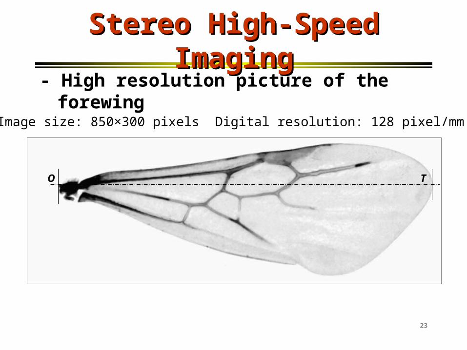
23
Stereo High-Speed ImagingStereo High-Speed Imaging- High resolution picture of the forewing
O T
Image size: 850×300 pixels Digital resolution: 128 pixel/mm

24
Stereo High-Speed ImagingStereo High-Speed Imaging- High resolution picture of the hindwing
O T
LH
Gray value distribution: G(L,H)
Image size: 850×300 pixels Digital resolution: 128 pixel/mm

25
Stereo High-Speed ImagingStereo High-Speed Imaging- Simulating images form three view angles
(x,y,z)H
L
gf(x,y)=G(L,H)
Front view image:
gs(z,y)=G(L,H)
Side view image:
gt(x,z)=G(L,H)
Top view image:

26
Stereo High-Speed ImagingStereo High-Speed Imaging- Original (top) and simulated (bottom) images

27
Stereo High-Speed ImagingStereo High-Speed Imaging- Reconstructed 3D view of the male
28
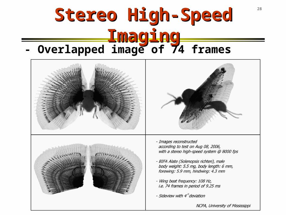
Stereo High-Speed ImagingStereo High-Speed Imaging- Overlapped image of 74 frames

29
Stereo High-Speed ImagingStereo High-Speed Imaging
– Reference
• Gui L, Fink T, Cao Z, Sun D, Seiner JM and Streett DA (2010) Fire ant alate wingmotion data and numerical reconstruction. Journal of Insect Science 10:9,available online: http://insectscience.org/10.19