10.3233@JAE-2010-1062

7/26/2019 10.3233@JAE-2010-1062

http://slidepdf.com/reader/full/103233jae-2010-1062 1/19

International Journal of Applied Electromagnetics and Mechanics 32 (2010) 1–19 1DOI 10.3233/JAE-2010-1062IOS Press

Numerical modeling of electromagneticwelding

S.D. Korea,∗, P. Dhaneshb, S.V. Kulkarnic and P.P. Dateba Mechanical Engineering Department, IIT Guwahati, Guwahati, 781039, Assam, Indiab Mechanical Engineering Department, IIT Bombay, Powai, Mumbai, 400076, Maharashtra, Indiac Electrical Engineering Department, IIT Bombay, Powai, Mumbai, 400076, Maharashtra, India

Abstract. Feasibility of electromagnetic welding of flat sheets is ascertained by comparing the minimum impact velocitiesdetermined by using software ANSYS/EMAG and ABAQUS with the required minimum velocity obtained from analyticalconsiderations. Magnetic forces acting on the sheets are computed from ANSYS/EMAG simulations. The velocity of impactand thepressureprofile actingon thesheets arefound from ABAQUS simulations. A criterion forweld formation is subsequentlyarrived at based on the simulations, which is further validated using experimental results. The reasons for no-weld zone inAl-to-Al EM weld and complete metal continuity (absence of no-weld zone) in Al-to-SS EM weld have been analyzed basedon the numerical and experimental results.

Keywords: Electromagnetic, welding, modeling

1. Introduction

Electromagnetic (EM) welding is a process of joining two similar or dissimilar metals by removingoxide layer and by creating a high velocity impact by Lorentz forces generated due to the electromagnetic

field and damped sinusoidal transient current. Electromagnetic welding of axis-symmetric components(tubes) has been established by many researchers [1–9]. The EM welding of flat sheets is cumbersomedue to the difficulty in controlling the magnetic field. Few researchers have reported the EM welding of Flat sheets [10–17]. The EM welding of Al-to-Al, Al-to-Cu, Al-to-SS, Cu-to-SS, Cu-to-Cu, Mg to Aland Al-to-Al-Li flat sheets has recently been established [18–20].

Complex EM field analysis is essential to decide the optimum parameters like current, frequency,inductance, and dimensions of the coil and work-piece. A numerical simulation can allow optimumdesign of a suitable coil and selection of optimum process parameters. Finite element modeling of the EM welding process is quite difficult due to its complex nature. It requires tight coupling of theelectromagnetic and structural models. Published literature on numerical modeling of EM welding of flat

sheets is scarce. Recently few researchers have reported the simulation-based approach for determiningthe impact velocity in EM welding process [17]. Electromagnetic welding of Al-to-Al sheets has shownno-weld zone at the centre whereas EM welding of Al-to-SS sheets with Al driver has shown continuousEM weld without any no-weld zone at the centre [13–15]. It is required to understand the effect of driver

on the occurrence of no-weld zone in the EM weld with the help of numerical simulations. Authors have

∗Corresponding author. E-mail: [email protected].

1383-5416/10/$27.50 © 2010 – IOS Press and the authors. All rights reserved

7/26/2019 10.3233@JAE-2010-1062


2 S.D. Kore et al. / Numerical modeling of electromagnetic welding

Al Plates

Coil

Coil

Switch

Capacitor Bank

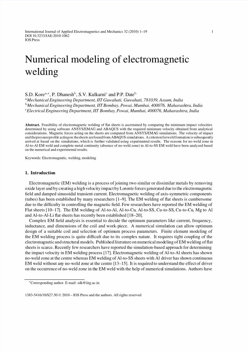
Fig. 1. Schematic representation of EM impact welding equipment.

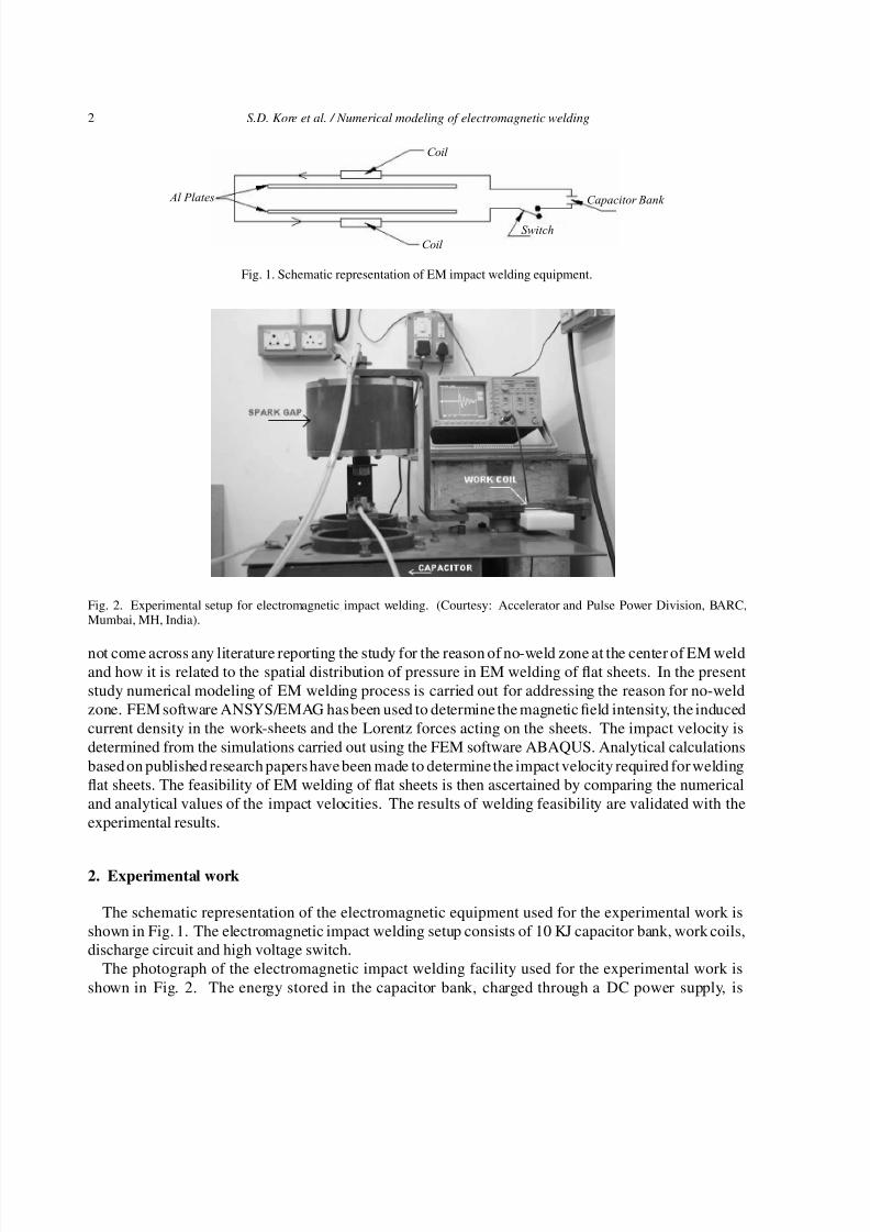
Fig. 2. Experimental setup for electromagnetic impact welding. (Courtesy: Accelerator and Pulse Power Division, BARC,Mumbai, MH, India).

not come across any literature reporting the study for the reason of no-weld zone at the center of EM weldand how it is related to the spatial distribution of pressure in EM welding of flat sheets. In the presentstudy numerical modeling of EM welding process is carried out for addressing the reason for no-weldzone. FEM software ANSYS/EMAG has been used to determine the magnetic field intensity, the inducedcurrent density in the work-sheets and the Lorentz forces acting on the sheets. The impact velocity isdetermined from the simulations carried out using the FEM software ABAQUS. Analytical calculations

based on published research papers have been made to determine the impact velocity required for weldingflat sheets. The feasibility of EM welding of flat sheets is then ascertained by comparing the numericaland analytical values of the impact velocities. The results of welding feasibility are validated with theexperimental results.

2. Experimental work

The schematic representation of the electromagnetic equipment used for the experimental work isshown in Fig. 1. The electromagnetic impact welding setup consists of 10 KJ capacitor bank, work coils,discharge circuit and high voltage switch.

The photograph of the electromagnetic impact welding facility used for the experimental work is

shown in Fig. 2. The energy stored in the capacitor bank, charged through a DC power supply, is

7/26/2019 10.3233@JAE-2010-1062


S.D. Kore et al. / Numerical modeling of electromagnetic welding 3

discharged through the work-coil by triggering the spark-gap. The damped sinusoidal current set up in

the work-coil produces a transient magnetic field. The work-sheets in the vicinity of the work-coil cut

the transient magnetic field. Hence, the induced electromotive force and the corresponding eddy currents

in the work-sheets oppose their cause. The induced eddy currents depend upon the material propertiessuch as conductivity and permeability. Finally, the work sheets are repelled away from the coil (towards

each other) creating an impact, due to Lorentz force, which lasts for a few microseconds, on account of

the interaction between the induced eddy currents and the magnetic field.

Welding requires atomically clean surfaces to be pressed together to obtain metallurgical continuity.

This continuity is hindered by oxides, adsorbed gases and surface contamination. Jetting phenomenon

due to high velocity impact causes the expulsion of the oxides on the surface of the colliding work-

sheet surfaces. After the collision, the atomically clean work-sheet surfaces are brought in contact by

pressing them together by electromagnetic pressure. The weld is formed at the interface establishing

the metallurgical continuity. The energy of the impact and hence the occurrence of the weld depends

on parameters such as inductance of the circuit, frequency, capacitor bank energy, voltage, current,

and standoff distance between the work-sheets. The standoff distance is the distance by which the

work-sheets to be welded are separated from each other prior to the energy discharge.

Authors have reported a detailed discussion about the experimental feasibility of EM welding of Al-to-

Al and Al-to-SS sheets in the previous papers [14,15]. Al-to-Al EM weld has shown the no-weld zone at

the centre whereas Al-to-SS EM weld show complete metal continuity without any no-weld zone at the

centre. It is reported that the centrally acting Lorentz force is the reason for no-weld zone at the centre

for Al-to-Al EM weld [14]. In case of Al-to-SS sheets EM welds are obtained by using Al driver to drive

the SS sheets. Due to this, centrally acting Lorentz force has dominating shear component which led to

continuous weld without any no-weld zone at the centre [15]. The reason for this no-weld condition is

studied in detail and validated with numerical simulations and analytical calculations in this paper.

3. Modeling in ANSYS

The EM welding process was modeled using a 2D linear transient magnetic analysis. The analytical

calculations determined the impact velocity required for the welding. Transient magnetic analysis

technique was used for calculating magnetic fields that vary over time. In this transient magnetic

analysis, the quantities analyzed were:

– current flow through the coil circuit,

– eddy currents generated in the sheets,

– magnetic flux density distribution, and

– magnetic forces acting on the sheets.

The simulation procedure involved creating a physics environment, building the model, assigning at-

tributes to the model regions, meshing the model, applying boundary conditions and loads, obtaining a

solution, and finally, analysis of the results.

Skin depth in copper coil at the set frequency (18.5 kHz) was equal to 0.48 mm. A single turn copper

work coil (5 mm × 0.48 mm) and an Al work sheet were modeled in two dimensions as shown in

Fig. 3. A rectangle of dimension (400 mm × 300 mm), which enclosed the coil/sheet system, was used

to model the surrounding free space. The resistivity of copper and Al assigned to the coil and sheets

respectively were 1.7 × 10−8 ohm-m and 2.77 × 10−8 ohm-m respectively.

7/26/2019 10.3233@JAE-2010-1062



Coil

Sheets

Coil

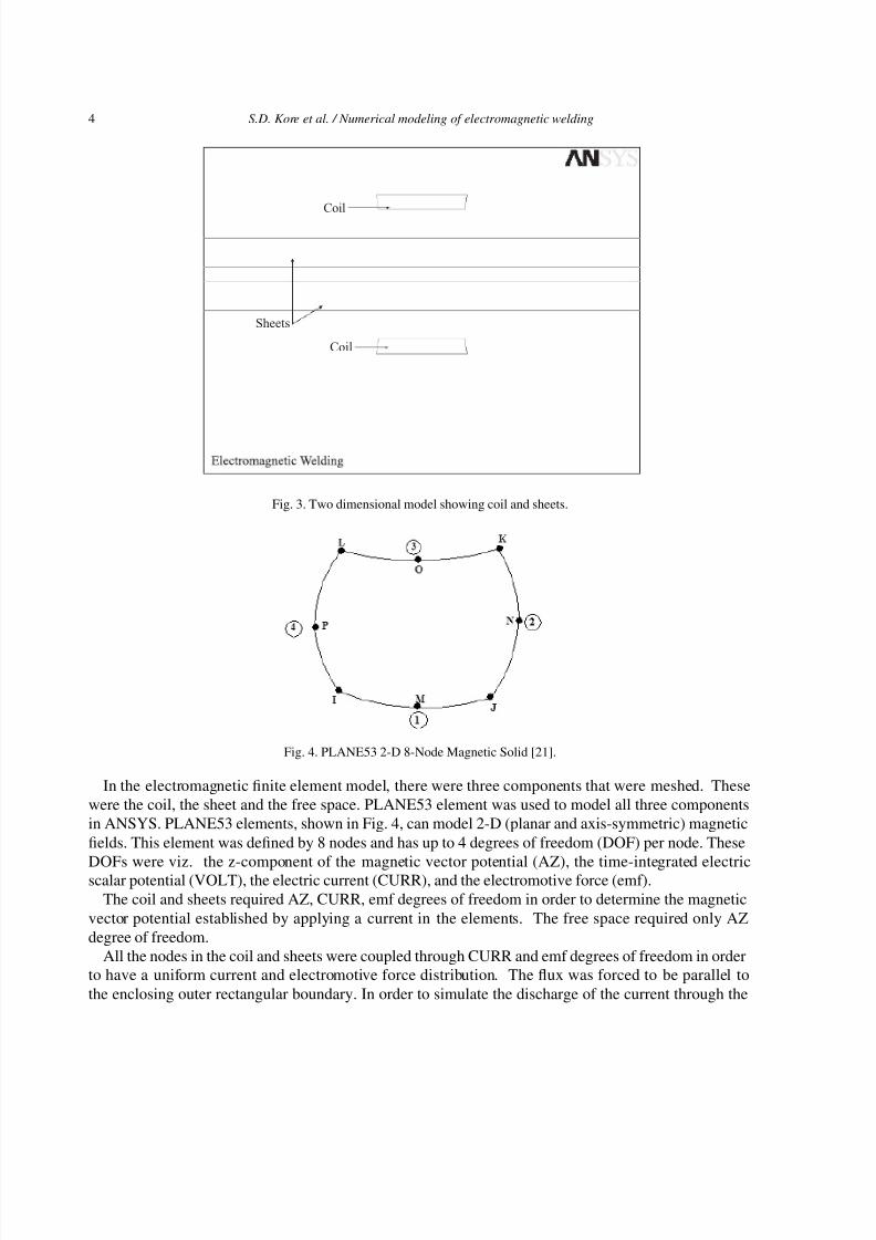
Fig. 3. Two dimensional model showing coil and sheets.

Fig. 4. PLANE53 2-D 8-Node Magnetic Solid [21].

In the electromagnetic finite element model, there were three components that were meshed. Thesewere the coil, the sheet and the free space. PLANE53 element was used to model all three componentsin ANSYS. PLANE53 elements, shown in Fig. 4, can model 2-D (planar and axis-symmetric) magnetic

fields. This element was defined by 8 nodes and has up to 4 degrees of freedom (DOF) per node. These

DOFs were viz. the z-component of the magnetic vector potential (AZ), the time-integrated electricscalar potential (VOLT), the electric current (CURR), and the electromotive force (emf).The coil and sheets required AZ, CURR, emf degrees of freedom in order to determine the magnetic

vector potential established by applying a current in the elements. The free space required only AZdegree of freedom.

All the nodes in the coil and sheets were coupled through CURR and emf degrees of freedom in orderto have a uniform current and electromotive force distribution. The flux was forced to be parallel to

the enclosing outer rectangular boundary. In order to simulate the discharge of the current through the

7/26/2019 10.3233@JAE-2010-1062



Fig. 5. CIRCU124 Coupled circuit source options [21].

Current Offset

Current Amplitude

Delay Time

Decay Factor

Fig. 6. Sinusoidal pulse applied to the current source.

coil, a current signal was fed to the coil elements by coupling them with the external circuit comprising

of the independent current source using CIRCU124 elements. CIRCU124 is a general circuit element

applicable to circuit simulation. The element interfaces with the electromagnetic finite elements to

simulate a coupled electromagnetic-circuit field interaction. The element has up to 6 nodes to define

a circuit component and up to three degrees of freedom per node to model circuit response. For the

modeling of EM welding process through such electromagnetic-circuit field coupling, the CIRCU124

element was interfaced with PLANE53 elements. CIRCU124 element was defined by active and passive

circuit nodes. Active nodes were those connected to an electric circuit while passive nodes were those

used internally by the elements and not connected to the circuit. In the current coupled circuit source

option, the passive nodes were the actual nodes of a coil modeled in the electromagnetic field domain.

A circuit, with CIRCU124 elements as shown in Fig. 5, consisting of independent current source and

standard coils, was used to feed the damped transient sinusoidal current through the work coil.

The independent current source was excited by an AC sinusoidal pulse by assigning the appropriate

key options like current offset, current amplitude, frequency, etc. as shown in Fig. 6.

7/26/2019 10.3233@JAE-2010-1062



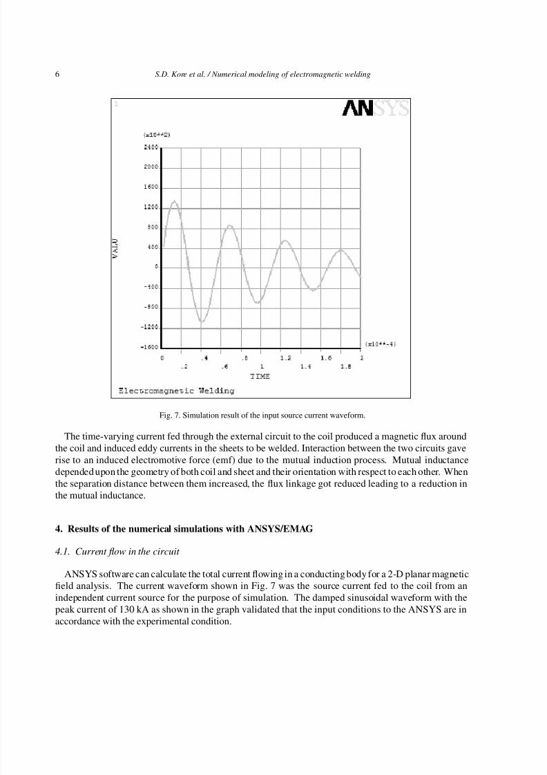
Fig. 7. Simulation result of the input source current waveform.

The time-varying current fed through the external circuit to the coil produced a magnetic flux aroundthe coil and induced eddy currents in the sheets to be welded. Interaction between the two circuits gaverise to an induced electromotive force (emf) due to the mutual induction process. Mutual inductancedepended upon the geometry of both coil and sheet and their orientation with respect to each other. Whenthe separation distance between them increased, the flux linkage got reduced leading to a reduction inthe mutual inductance.

4. Results of the numerical simulations with ANSYS/EMAG

4.1. Current flow in the circuit

ANSYS software can calculate the total current flowing in a conducting body for a 2-D planar magneticfield analysis. The current waveform shown in Fig. 7 was the source current fed to the coil from anindependent current source for the purpose of simulation. The damped sinusoidal waveform with thepeak current of 130 kA as shown in the graph validated that the input conditions to the ANSYS are inaccordance with the experimental condition.

7/26/2019 10.3233@JAE-2010-1062



Fig. 8. Contour plot of magnetic flux.

4.2. Contour plot of 2D flux lines

The flux developed by the damped sinusoidal current is depicted in Fig. 8. It shows the plot of theequi-potential lines of AZ. These equi-potential lines are actually also the flux lines in this 2D case andthus, give us a good picture of the flux patterns. The contours are in accordance with the theoretical formof the flux pattern.

4.3. Magnetic flux density

The magnetic flux density for the numerical simulation is shown in Fig. 9 and its maximum value isfound to be 30 Tesla. The analytically calculated value of the magnetic flux density is about 33 T (usingEq. (1)) [10].

B = µI [tan−1

b/2d1

+ tan−1

b/2d2

]

πb (1)

The values of d1 and d2 in Eq. (1) are determined for the initial position of the sheets with respect tothe coil, i.e., position of sheets before collision. The values of d 1 and d2, determined using the initial

position of the sheets with respect to the coils, i.e., at the time of collision, are given below.where, I = discharge current; A,b = width of the middle ‘I’ shaped web portions of the coil; = 5 mm,d1, d2 = distances of the sheets from the inner surfaces of the upper and lower ‘I’ shaped web of the

coil respectively; mAt initial position of the sheet, d1 = d2 = 0.07 × 10−3 mThe contour plot shows that the penetration of the magnetic field through the sheets was negligible.

This means that maximum amount of magnetic field was available for inducing the current in the sheets.

7/26/2019 10.3233@JAE-2010-1062



Fig. 9. Vector plot of magnetic flux.

4.4. Current density in the sheets

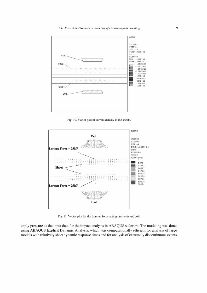
The Al sheets, kept in the vicinity of the work coil, cut the magnetic field developed and a current gotinduced in the sheets. Figure 10 shows the vector plot of the induced eddy current densities in the sheet.It has shown that the induced current density pattern and magnitude were the same for Al sheets. Thecurrent density was maximum on the surfaces of sheets facing the coil due to the skin depth phenomenon.

4.5. EM lorentz forces acting on the sheet

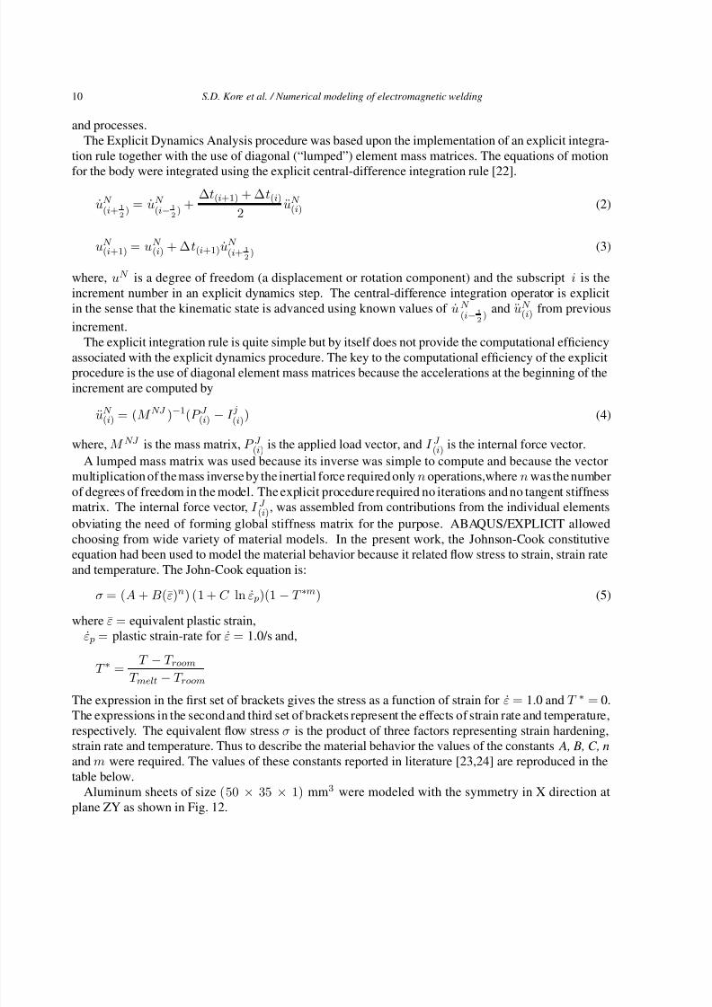
The EM Lorentz forces are shown in Fig. 11. The value of the Lorentz force was found to be 25 kN,which was acting on the sheet area exactly opposite to the coil area. The force pattern showed that thedirection of the force was normal at the centre whereas it had some shear component away from thecentre. The normal component of the force was dominant at the centre whereas the shear componentwas dominant at the edges. The normally acting force resulted in a rebounding effect leading to no-weld

region in the centre of the weld. The shear component at the edges helped in expelling out the oxidesand creating the weld.

5. Numerical simulations to determine the velocity of impact

ABAQUS 6.6-3 commercial software was used for determining the velocity by numerical modelingof the EM welding process. The magnetic force obtained from the ANSYS/EMAG analysis was used to

7/26/2019 10.3233@JAE-2010-1062



Fig. 10. Vector plot of current density in the sheets.

Fig. 11. Vector plot for the Lorentz force acting on sheets and coil.

apply pressure as the input data for the impact analysis in ABAQUS software. The modeling was done

using ABAQUS Explicit Dynamic Analysis, which was computationally efficient for analysis of large

models with relatively short dynamic response times and for analysis of extremely discontinuous events

7/26/2019 10.3233@JAE-2010-1062



and processes.The Explicit Dynamics Analysis procedure was based upon the implementation of an explicit integra-

tion rule together with the use of diagonal (“lumped”) element mass matrices. The equations of motion

for the body were integrated using the explicit central-difference integration rule [22].

uN (i+ 1

2) = uN

(i−1

2) +

∆t(i+1) + ∆t(i)

2 uN

(i) (2)

uN (i+1) = uN

(i) + ∆t(i+1) uN (i+ 1

2)

(3)

where, uN is a degree of freedom (a displacement or rotation component) and the subscript i is theincrement number in an explicit dynamics step. The central-difference integration operator is explicitin the sense that the kinematic state is advanced using known values of uN

(i−1

2)

and uN (i) from previous

increment.The explicit integration rule is quite simple but by itself does not provide the computational efficiency

associated with the explicit dynamics procedure. The key to the computational efficiency of the explicitprocedure is the use of diagonal element mass matrices because the accelerations at the beginning of theincrement are computed by

uN (i) = (M NJ )−1(P J (i) − I

j

(i)) (4)

where, M NJ is the mass matrix, P J (i) is the applied load vector, and I J (i) is the internal force vector.

A lumped mass matrix was used because its inverse was simple to compute and because the vectormultiplication of the mass inverse by the inertial force required onlyn operations,where nwasthe number

of degrees of freedom in the model. The explicit procedure required no iterations and no tangent stiffnessmatrix. The internal force vector, I J (i), was assembled from contributions from the individual elements

obviating the need of forming global stiffness matrix for the purpose. ABAQUS/EXPLICIT allowedchoosing from wide variety of material models. In the present work, the Johnson-Cook constitutiveequation had been used to model the material behavior because it related flow stress to strain, strain rateand temperature. The John-Cook equation is:

σ = (A+B(ε)n) (1 + C ln ε p)(1 − T ∗m) (5)

where ε = equivalent plastic strain,ε p = plastic strain-rate for ε = 1.0/s and,

T ∗ = T − T room

T melt − T room

The expression in the first set of brackets gives the stress as a function of strain for ε = 1.0 and T

∗

= 0.The expressions in the second and third set of brackets represent the effects of strain rate and temperature,respectively. The equivalent flow stress σ is the product of three factors representing strain hardening,strain rate and temperature. Thus to describe the material behavior the values of the constants A, B, C, n

and m were required. The values of these constants reported in literature [23,24] are reproduced in thetable below.

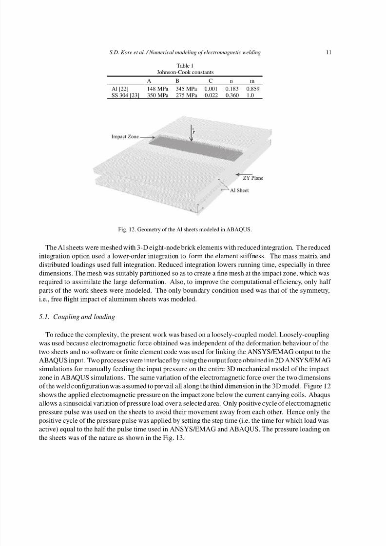
Aluminum sheets of size (50 × 35 × 1) mm3 were modeled with the symmetry in X direction atplane ZY as shown in Fig. 12.

7/26/2019 10.3233@JAE-2010-1062



Table 1Johnson-Cook constants

A B C n m

Al [22] 148 MPa 345 MPa 0.001 0.183 0.859

SS 304 [23] 350 MPa 275 MPa 0.022 0.360 1.0

Fig. 12. Geometry of the Al sheets modeled in ABAQUS.

The Al sheets were meshed with 3-D eight-node brick elements with reduced integration. The reduced

integration option used a lower-order integration to form the element stiffness. The mass matrix and

distributed loadings used full integration. Reduced integration lowers running time, especially in three

dimensions. The mesh was suitably partitioned so as to create a fine mesh at the impact zone, which was

required to assimilate the large deformation. Also, to improve the computational efficiency, only half

parts of the work sheets were modeled. The only boundary condition used was that of the symmetry,

i.e., free flight impact of aluminum sheets was modeled.

5.1. Coupling and loading

To reduce the complexity, the present work was based on a loosely-coupled model. Loosely-coupling

was used because electromagnetic force obtained was independent of the deformation behaviour of the

two sheets and no software or finite element code was used for linking the ANSYS/EMAG output to the

ABAQUS input. Two processes were interlaced by using the output force obtained in 2D ANSYS/EMAG

simulations for manually feeding the input pressure on the entire 3D mechanical model of the impact

zone in ABAQUS simulations. The same variation of the electromagnetic force over the two dimensions

of the weld configuration was assumed to prevail all along the third dimension in the 3D model. Figure 12

shows the applied electromagnetic pressure on the impact zone below the current carrying coils. Abaqus

allows a sinusoidal variation of pressure load over a selected area. Only positive cycle of electromagnetic

pressure pulse was used on the sheets to avoid their movement away from each other. Hence only the

positive cycle of the pressure pulse was applied by setting the step time (i.e. the time for which load was

active) equal to the half the pulse time used in ANSYS/EMAG and ABAQUS. The pressure loading on

the sheets was of the nature as shown in the Fig. 13.

7/26/2019 10.3233@JAE-2010-1062



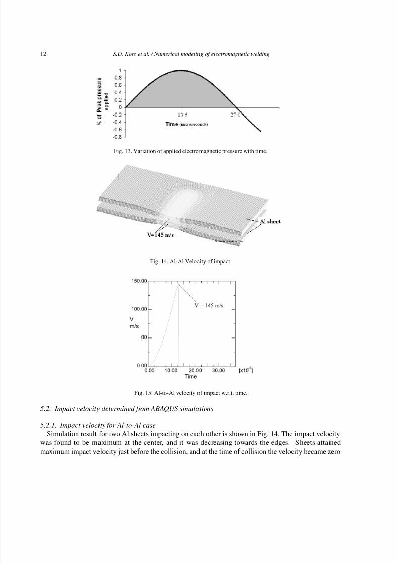
Fig. 13. Variation of applied electromagnetic pressure with time.

Fig. 14. Al-Al Velocity of impact.

Fig. 15. Al-to-Al velocity of impact w.r.t. time.

5.2. Impact velocity determined from ABAQUS simulations

5.2.1. Impact velocity for Al-to-Al case

Simulation result for two Al sheets impacting on each other is shown in Fig. 14. The impact velocitywas found to be maximum at the center, and it was decreasing towards the edges. Sheets attained

maximum impact velocity just before the collision, and at the time of collision the velocity became zero

7/26/2019 10.3233@JAE-2010-1062



Fig. 16. Al-to-SS velocity of impact.

Fig. 17. Al-SS velocity of impact w.r.t. time.

as shown in Fig. 15. For Al-to-Al sheets the velocity of impact at 25 kN magnetic force was found to be

145 m/s from the simulation.

5.2.2. mpact velocity for Al-to-SS case

Simulation result for two Al and SS sheets impacting on each other is shown in Fig. 16. Al driverwas used to drive the electrically poor conducting SS sheet. Just before the collision, sheets attained

maximum velocity as shown in Fig. 17. For Al-to-SS sheets the velocity of impact at 30 kN magnetic

force was found to be 139 m/s. After the impact, welded sheets showed vibration due to instability in air.

5.3. Analytical calculations for velocity

Due to similarity of the EM and explosive welding techniques, and non-availability of any criterion forthe EM welding, explosive welding criterion was adopted to obtain the weldability condition for differentmaterial combinations. A detailed analysis and discussion about the explosive welding criterion can be

found in [25,26].

7/26/2019 10.3233@JAE-2010-1062



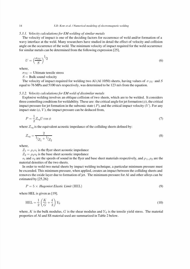
5.3.1. Velocity calculations for EM welding of similar metals

The velocity of impact is one of the deciding factors for occurrence of weld and/or formation of a

wavy interface at the weld. Many researchers have studied in detail the effect of velocity and collision

angle on the occurrence of the weld. The minimum velocity of impact required for the weld occurrencefor similar metals can be determined from the following expression [25],

U =σTU S

1/2(6)

where,

σTU = Ultimate tensile stress

S = Bulk sound velocity

The velocity of impact required for welding two Al (Al 1050) sheets, having values of σ TU and S

equal to 76 MPa and 5100 m/s respectively, was determined to be 123 m/s from the equation.

5.3.2. Velocity calculations for EM weld of dissimilar metalsExplosive welding involves an oblique collision of two sheets, which are to be welded. It considers

three controlling conditions for weldability. These are: the critical angle for jet formation (φ), the critical

impact pressure for jet formation in the subsonic state (P ), and the critical impact velocity (V ). For any

impact state (φ, V ), the impact pressure can be deduced from,

P = 1

2Z eqU cos φ (7)

where Z eq is the equivalent acoustic impedance of the colliding sheets defined by:

Z eq = 2

1/

Z 1 + 1/

Z 2

(8)

where,

Z 1 = ρ1s1 is the flyer sheet acoustic impedanceZ 2 = ρ2s2 is the base sheet acoustic impedances1 and s2 are the speeds of sound in the flyer and base sheet materials respectively, and ρ 1, ρ2 are the

material densities of the two sheets.

In order to weld two metal sheets by impact welding technique, a particular minimum pressure must

be exceeded. This minimum pressure, when applied, creates an impact between the colliding sheets and

removes the oxide layer due to formation of jet. The minimum pressure for Al and other alloys can beestimated by [25,26]:

P = 5 × Hugoniot Elastic Limit (HEL) (9)

where HEL is given as [19],

HEL = 1

2

K

G +

4

3

Y 0 (10)

where, K is the bulk modulus, G is the shear modulus and Y 0 is the tensile yield stress. The material

properties of Al and SS material used are summarized in Table 2 below.

7/26/2019 10.3233@JAE-2010-1062



Table 2Material properties of Al and SS [26]

Sr.No Material Density Bulk modulus, Shear modulus, Tensile yield Speed of sound,(kg/m3) K , (GPa) G, (GPa) stress, Y 0 (MPa) S , (m/s)

1 Al 2700 76 26 28 51002 SS 8000 120 90 215 5130

Table 3Comparison of impact velocities

Sr Material Size (mm3) Minimum velocity required Impact velocity determinedNo for impact welding, from numerical simulations

determined from using ANSYS/ literature [24,25] EMAG and ABAQUS

1 Al-Al 50 × 100× 1 123 m/s 145 m/s2 Al-SS (with SS-50 × 50× 0.25 136 m/s 139 m/s

Al driver) Al-50 × 100 × 1

Fig. 18. Al-Al EM weld showing maximum negative pressure at the centre leading to no-weld zone.

The estimated values of impact velocities for welding Al-to-Al and Al-to-SS by numerical simulationusing ANSYS/EMAG were 145 m/s and 139 m/s respectively. The values of velocities of impact requiredfor welding Al-to-Al and Al-to-SS derived from analytical calculations Eqs (7–10) were 123 m/s and136 m/s respectively. Thus, the velocities obtained by simulation are higher than the required minimumvalues, and hence the feasibility of the weld creation was verified analytically, which corroborates wellwith the previously published experimental results [14,15]. The results are summarized in Table 3.

6. Spatial variation of pressure

6.1. Al-to-Al sheets

Figure 18 shows simulation result for the variation in pressure along the impact zone. It was found,for the case of Al-to-Al sheets, that the negative pressure (pressure acting away from collision direction)acting was maximum along the central line. This was due to the restitution effect being maximum at

7/26/2019 10.3233@JAE-2010-1062



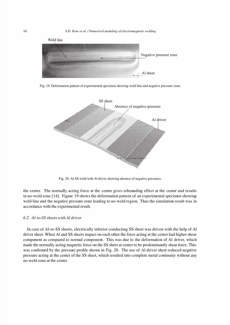
Fig. 19. Deformation pattern of experimental specimen showing weld line and negative pressure zone.

Fig. 20. Al-SS weld with Al driver showing absence of negative pressures.

the center. The normally acting force at the center gives rebounding effect at the center and results

in no-weld zone [14]. Figure 19 shows the deformation pattern of an experimental specimen showing

weld line and the negative pressure zone leading to no-weld region. Thus the simulation result was in

accordance with the experimental result.

6.2. Al-to-SS sheets with Al driver

In case of Al-to-SS sheets, electrically inferior conducting SS sheet was driven with the help of Aldriver sheet. When Al and SS sheets impact on each other the force acting at the center had higher shear

component as compared to normal component. This was due to the deformation of Al driver, which

made the normally acting magnetic force on the SS sheet at center to be predominantly shear force. This

was confirmed by the pressure profile shown in Fig. 20. The use of Al driver sheet reduced negative

pressure acting at the center of the SS sheet, which resulted into complete metal continuity without any

no-weld zone at the center.

7/26/2019 10.3233@JAE-2010-1062



Fig. 21. Al-to-Al sheets with Al driver showing absence of negative pressure.

6.3. Al-to-Al sheets with Al driver

Although Al being electrically good conducting material, a simulation of Al-to-Al impact was carriedout with using Al driver to confirm the finding that the driver sheet changed the pressure profile andresulted into complete metal continuity without any no-weld zone at the center. The result obtained fromthe simulation with combined ANSYS/EMAG and ABAQUS is shown in Fig. 21. It confirmed that incase of Al-to-Al sheets if we use driver sheet of Al the negative pressure at the center is absent, whichresults into complete metal continuity without any no-weld zone.

Thus the normally acting force at the center was the reason for negative pressure and in turn for the

corresponding no-weld zone. In the present analysis the effect of oxide layer was ignored, which wasalso one of the vital factors for no-weld zone at the center for Al [14].

7. Conclusions

Feasibility of EM welding of flat sheets has been successfully established by comparing velocityof impact determined using ANSYS/EMAG and ABAQUS softwares and minimum impact velocityestimated from analytical calculations. The numerical simulation results for the EM weld feasibilitywere in accordance with the previously published experimental results [14,15].

Spatial pressure distribution on sheets determined from numerical simulation was in agreement withthe experimental results. It is confirmed from the numerical simulation results that normally acting force

at the center is the reason for no-weld zone at the centre in Al-to-Al EM weld. Restitution effect, beingmaximum at the center, has created negative pressure giving rebounding effect and resulted in no-weldzone. Due to the use of Al driver in case of Al-to-SS sheets the normally acting force has dominatingshear component at centre and produced continuous EM welds without any no-weld zone.

In future, numerical simulations can be carried out for three dimensional models of the coil and sheetswith strong coupling between the electromagnetic and structural code by using the softwares like LSDyna. The impact velocity can be measured and compared with the numerical results to validate thenumerical models.

7/26/2019 10.3233@JAE-2010-1062



Acknowledgements

Authors thank Dr. R.C. Sethi Former Head, APPD, BARC, Mr. D.P. Chakravarty Head APPD, BARC

and Dr. K.V. Nagesh, Head EPPS, APPD, BARC, for kindly permitting the use of the experimentalfacility available at BARC. Authors also thank Mr. S.V. Desai, Mr. R.K. Rajawat, Mr. M.R. Kulkarni,

Ms. Dolly Rani and Mr. Satendra Kumar from APPD, BARC for their valuable suggestions and help

while conducting the experiments. Authors thank Dr. Ganesh Kumbhar for his vital help for numerical

simulations in ANSYS/ EMAG.

References

[1] P. Zhang, Joining enabled by high velocity deformation, Ph.D. Thesis, Ohiostate university, available on-line at http://mse-gsd1.matsceng.ohio-state.edu/˜glenn/HRFSUP/P Zhang PhD 2003.pdf as on April 11, 2009.

[2] P. Zhang, M. Kimchi, H. Shao, J.E. Gould and G.S. Daehn, Analysis of the electromagnetic impulse joining process witha field concentrator, Numiform, 2004, 1253-58.

[3] I. Masumoto, K. Tamaki and M. Kojima, Electromagnetic welding of aluminum tube to aluminum or dissimilar metalcores, Transactions on Japan Welding Society 2(16) (1985), 110–116.

[4] M. Marya and S. Marya, Interfacial microstructures and temperatures in aluminum – copper electromagnetic pulse welds.Sci Technol, Weld Joining 9(6) (2004), 541–547.

[5] A. Stern and M. Aizenshtein, Bonding zone formation in magnetic pulse welds, Sci Technol Weld Joining 7(5) (2002),339–342.

[6] M. Marya, S. Marya and D. Priem, On the characteristics of electromagnetic welds between aluminum and other metalsand alloys, Weld World (49) (2005), 74–84.

[7] V. Shribman, A. Stern, Y. Livshitz and O. Gafri, Magnetic pulse welding produces high strength aluminum welds, Weld J 81(4) (2002), 33–37.

[8] M. Kimchi, H. Saho, W. Cheng and P. Krishnaswamy, Magnetic pulse welding of aluminum tubes to steel bars, Weld World (48) (2004), 19–22.

[9] TWI knowledge summary, Magnetic pulse welding, TWI world center for material joining technology, available at,

http://www.twi.co.uk, as on April 11, 2009.[10] T. Aizawa, K. Okogawa, M. Yoshizawa and N. Henmi, Impulse magnetic pressure seam welding of aluminum sheets, Impact Engineering and Applications (2001), 827–832.

[11] T. Aizawa and K. Okogawa, Impact seam welding with magnetic pressure for Aluminum sheets, Material Science Forum465 (2004), 231–236.

[12] T. Aizawa, Methods for electromagnetic pressure seam welding of Al/Fe sheets, Welding International 18(11) (2004),868–872.

[13] S.D. Kore, P.P. Date and S.V. Kulkarni, Electromagnetic Welding of Al Sheets, Sheet Metal Welding Conference XII,AWS, Livonia, Michigan, Detroit USA, 2006, 1–6.

[14] S.D. Kore, P.P. Date and S.V. Kulkarni, Effect of process parameters on electromagnetic impact welding of Al sheets, International Journal of Impact Engineering 34 (2007), 1327–1341.

[15] S.D. Kore, P.P. Date and S.V. Kulkarni, Electromagnetic impact welding of aluminum to stainless steel sheets, Journalof Materials Processing Technology 208 (2008), 486–493.

[16] Y. Zhang, S.S. Babu, P. Zhang, E.A. Kenik and G.S. Daehn, Microstructure characterisation of magnetic pulse weldedAA6061-T6 by electron backscattered diffraction, Science and Technology of Welding Joining 13(5) (2008), 467–471.

[17] Y. Zhang, P.L. Eplattenier, T. Geoff, A. Vivek, G. Daehn and S. Babu, Numerical Simulation and Experimental Study for Magnetic Pulse Welding Process on AA6061 and Cu 101 Sheet , 10th International LSDyna Users conference, 2008.[18] S.D. Kore, Ph.D. Thesis, Mechanical Engineering Department, Indian Institute of Technology, Bombay, January 2008.[19] S.D. Kore, P.P. Date, S.V. Kulkarni, S. Kumar, M.R. Kulkarni, S.V. Desai, R.K. Rajawat, K.V. Nagesh and D.P.

Chakravarty, Electromagnetic Impact Welding of Al-to-Al-Li Sheets, accepted for publication in Journal of ManufacturingScience and Engineering, ASME, on January 13, 2009.

[20] S.D. Kore, J. Imbert, M.J. Worswick and Y. Zhou, Electromagnetic Impact Welding of Mg to Al Sheets, Science andTechnology of Welding and Joining, Vol. 14, No. 6, pp. 549–553.

[21] Ansys (9) Theory Manual. Inc, 2007.[22] ABAQUS 6.6-3 Theory Manual.

7/26/2019 10.3233@JAE-2010-1062



[23] N.K. Gupta, M.A. Iqbal and G.S. Sekhon, Experimental and numerical studies on the behavior of thin aluminum platessubjected to impact by blunt- and hemispherical-nosed projectiles, International Journal of Impact Engineering 32(2006), 1921–1944.

[24] A.A. Akbari Mousavi and S.T.S. Al-Hassani, Finite Element simulation of Explosive-driven plate impact with application

to explosive welding, Materials and Design 29(1) (2008), 1–19.[25] T.Z. Blazynski, ed., Explosive Welding, Forming, and Compaction. Elsevier Science: New York, 1983.[26] K.K. Botros and T.K. Groves, Fundamental impact parameters – an experimental investigation using a 76 mm powder

canon, Journal of Applied Physics 51(7) (1980), 3706–3714.[27] www.matweb.com as on April 11, 2009.

10.3233@JAE-2010-1062

Documents

Transcript of 10.3233@JAE-2010-1062