S) Production at DØDaniela Bauer, Jundong Huang,

Andrzej Zieminski

Indiana University

Why measure (1S) production at DØ ?

● Measuring the (1S) production cross-section provides an ideal testing ground for our understanding of the production mechanisms of heavy quarks. There is considerable interest from theorists in these kinds of measurements: E.L. Berger, J.Qiu, Y.Wang, Phys Rev D 71 034007 (2005) and hep-ph/0411026;

● Because we can: The (1S) cross-section had been measured at the Tevatron (Run I measurement by CDF) up to a rapidity of 0.4. DØ has now measured this cross-section up to a rapidity of 1.8 at √s = 1.96 TeV

V.A. Khoze , A.D. Martin, M.G. Ryskin, W.J. Stirling, hep-ph/0410020

The Analysis

● Opposite sign muons ● Muon have hits in all three layers of the muon system● Muons are matched to a track in the central tracking system● p

t (μ) > 3 GeV and |η (μ)| < 2.2

● At least one isolated muon● Track from central tracking system must have at least one hit in the Silicon Tracker

Goal: Measuring the (1S) cross-section in the channel (1S) → μ+μ- as a function of p

t in three rapidity ranges:

0 < | y| < 0.6, 0.6 < | y| < 1.2 and 1.2 < | y| < 1.8

Sample selection:

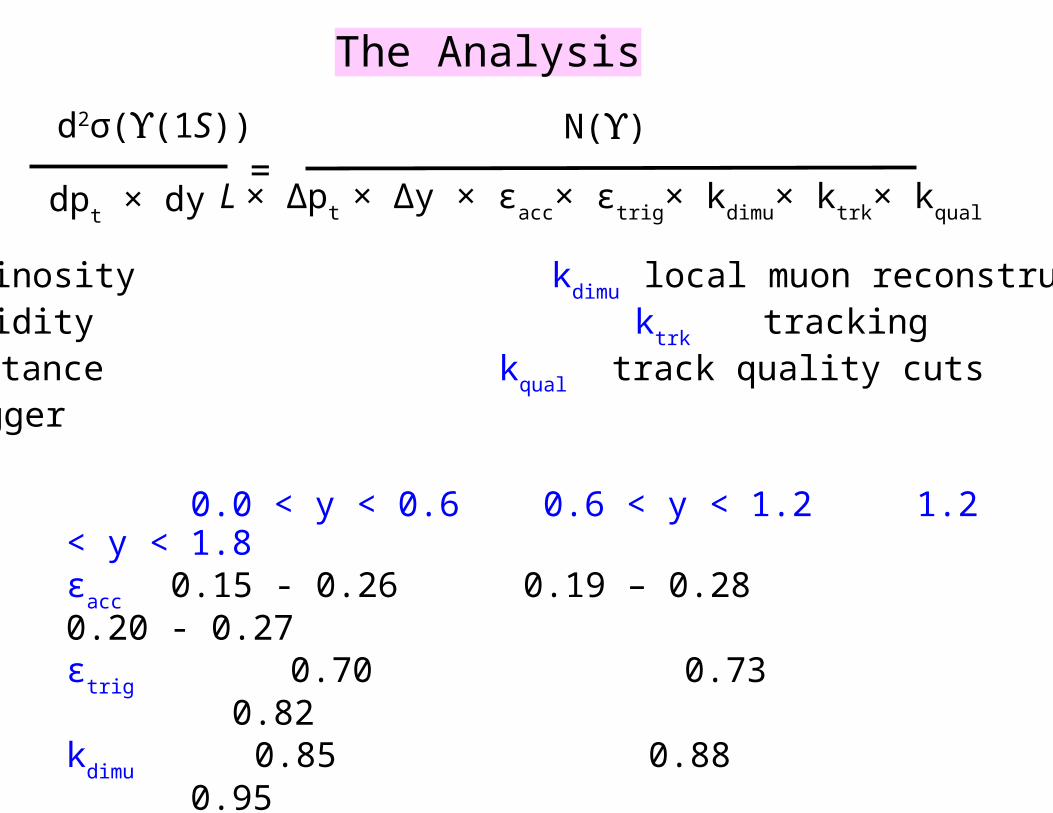
d2σ((1S))

dpt × dy

N()

L × Δpt × Δy × ε

acc× ε

trig× k

dimu× k

trk× k

qual

=

The Analysis

L Luminosity kdimu

local muon reconstructiony rapidity k

trk tracking

εacc

Acceptance kqual

track quality cuts ε

trig Trigger

0.0 < y < 0.6 0.6 < y < 1.2 1.2 < y < 1.8ε

acc 0.15 - 0.26 0.19 – 0.28 0.20 - 0.27

εtrig

0.70 0.73 0.82k

dimu 0.85 0.88 0.95

ktrk

0.99 0.99 0.95 k

qual 0.85 0.85 0.93

MC Data*

pt(μ)

in GeV

0 5 10 15 20 -2 -1 0 1 2 0 3 6

η(μ) φ(μ)

0.6 < | y| < 1.2*9.0 GeV < m(μμ) < 9.8 GeV

To determine our efficiencies, we only need an agreement between Monte Carlo and data within a give p

Tϒ and yϒ bin and not an agreement over the

whole pTϒ and yϒ range at once.

Data Monte carlo comparison

All plots: 4 GeV < pt( < 6 GeV

m() = 9.419 ± 0.007 GeV m() = 9.412 ± 0.009 GeV m() = 9.437 ± 0.010 GeV

0 < |y | < 0.6

Fitting the signal

0.6 < |y | < 1.2 1.2 < |y | < 1.8

m((2/3S)) = m((1S)) + ∆ mPDG

((2/3S)-(1S))

σ((2/3S)) = m((2/3S)/m((1S)) * σ((1S)) →5 free parameters in signal fit: m((1S)), σ((1S)), c((1S)), c((2S)), c((3S))

Signal: 3 Gaussians: (1S), (2S), (3S)

Background: 3rd order polynomial

PDG: m((1S)) = 9.460 GeV

Fitting a single Gaussianrecovers ~95 % of the signal.

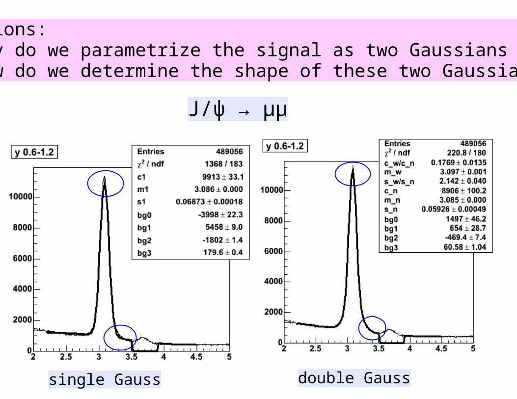
J/ψ → µµ

Questions:a) Why do we parametrize the signal as two Gaussians ?b) How do we determine the shape of these two Gaussians ?

single Gauss double Gauss

Question: Why do we use different fitting ranges for different bins ?

● The fit assumes a smooth background. We choose the fitting range accordingly.

ptϒ 1-2 GeV

yϒ 1.2 - 1.8 ● With increasing p

tϒ the mass

peaks widens, but background is better behaved→ increased fitting range

● We derive a systematic error from varying our fitting range.

Wid

th ϒ

(1S

)

0

0

.25

0

.5

Fitting - Results● The fitted width is ptindependent● The resolution is ~30%worse than in MC● The (relative) wideningof the peak in the forwardregion is reproduced by MC

Fitting - resultsRatio ofn((2S+3S))/n((1S)

Normalized differential cross section

There is very littledifference in shapeof the distribution asa function of the ϒ ϒrapidity.

Results: dσ(ϒ(1S))/dy × B(ϒ(1S)) → µ+µ-

0.0 < yϒϒ < 0.6 732 ± 19 (stat) ± 73 (syst) ± 48 (lum) pb

0.6 < yϒϒ < 1.2 762 ± 20 (stat) ± 76 (syst) ± 50 (lum) pb

1.2 < yϒϒ < 1.8 600 ± 19 (stat) ± 56 (syst) ± 39 (lum) pb

0.0 < yϒϒ < 1.8 695 ± 14 (stat) ± 68 (syst) ± 45 (lum) pb

CDF Run I: 680 ± 15 (stat) ± 18 (syst) ± 26 (lum) pb

Largest contribution to the systematic error is the uncertainty ondeterming kdimu, followed CDF can separate the three Upsilon states.

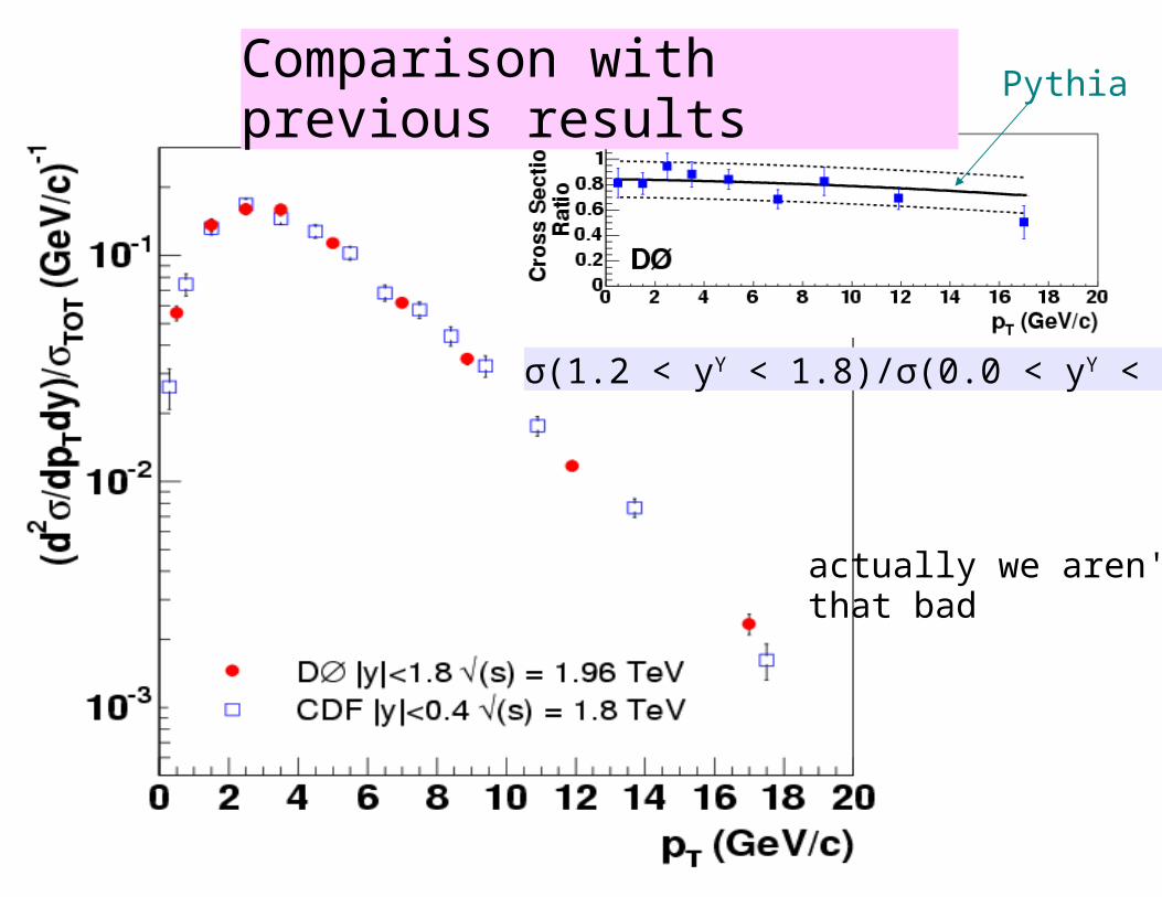
Comparison with previous results

σ(1.2 < yϒ < 1.8)/σ(0.0 < yϒ < 0.6)

Pythia

actually we aren't that bad

Questions: Why does the mass peak widen in the forward region ? How is the increased resulting smearing corrected in the cross section ?

● The tracking resolution is worse in the forward region, as the tracks have a higher momentum and intersect with the tracking detectors at an angle. ● This trend is reproduced in our Monte Carlo.● We increase the Monte carlo resolution by 30% over the default to match what we see in data.● The momentum scale is corrected for using the difference between measured and PDG ϒ(1S) mass.

Question: Does the mass resolution really scale with the mass of the particle ?

Yes. Both in data (compared to J/ψ →µµ) and in Monte-Carlo.

Questions: Do we understand the rapidity dependence of our correction factors k_qual and k_trk ?

k_qual: SMT hit requirement: If we do find a track in the forward region in data, itwill have an SMT hit, as there is nothing else to make a track. Therefore the SMT hit requirement affects the forward region less than the central region. Isolation: In MC the isolation requirement is 100% efficient, i.e. we do not loose any signal when applying it. In data we loose up to 6% of the signal, butconsiderably less in the forward region.

Track quality cuts: At least 1 SMT hit on each track. At least one of the tracks forming an ϒ has to be isolated.

k_trk (Tracking efficiency): The Monte-Carlo overestimates the trackingefficiency in the forward region as it does not take the faulty SMT disks into account.

Plot by Rob McCroskey

Question: What is the L1 trigger efficiency per muon ?

0 3 5 9 GeV

lo

g sc

ale

● We only determine the trigger efficiency for dimuons.

µ from ϒ(1S)

● Approximately half the muons from ϒ(1S) have a pt < 5 GeV.

● Trigger turn-on curve from Rob McCroskey

Question: CDF measured ϒ(1S) polarization for |yϒ| < 0.4. How can we be sure that our forward ϒ(1S) are not significantly polarized ?

● So far there is no indication for ϒ(1S) polarization. CDF measured α = -0.12 ± 0.22 for p

Tϒ > 8 GeV

α = 1 (-1) ⇔ 100% transverse (longitudinal) polarization The vast majority of our ϒ(1S) has p

Tϒ < 8 GeV

Theory predicts that if there is polarization it will be at large pT.

● We checked for polarization in our signal (|y| < 1.8) and found none. There is not enough data for a fit in the forward region alone.

● We estimated the effect of ϒ(1S) polarization on our cross-section. Even at α = ± 0.3 the cross-section changes by 15% or less in all pT bins. The effect is the same in all rapidity regions.

Question: Why is CDF's systematic error so much smaller than ours ?

● Better tracking resolution --- CDF can separate the three ϒ resonances: → Variations in the fit contribute considerable both to our statistical and systematic error. → We believe we have achieved the best resolution currently feasible without killing the signal.

● Poor understanding of our Monte-Carlo and the resulting large number of correction factors.

● Signal is right on the trigger turn-on curve.

Conclusions

● (1S) cross-section measurement extended to yϒ = 1.8.● First measurement of (1S) cross-section at √s = 1.96 TeV.

● Normalized cross-sections show very little dependence on rapidity.

● Normalized cross-section is in good agreement with published results.

Backup slides

Where do the (1S) come from ?

Bottomonium States

●of (1S) are produced directly.

● The rest are the result of higher mass states decaying.

GeV GeV GeV

All plots: 3 GeV < pt( < 4 GeV

m() = 9.423 ± 0.008 GeV m() = 9.415± 0.009 GeV m() = 9.403 ± 0.013 GeV

0 < |y | < 0.6

The signal

0.6 < |y | < 1.2

7 8 9 10 11 12 13 7 8 9 10 11 12 13 7 8 9 10 11 12 13

1.2 < |y | < 1.8

m((2/3S)) = m((1S)) + mPDG

((2/3S)-(1S))

σ ((2/3S)) = m((2/3S)/m((1S)) * σ σ ((1S)) →5 free parameters in signal fit: m((1S)), σ((1S)), c((1S)), c((2S)), c((3S))

Signal: 3 Gaussians: (1S), (2S), (3S)

Background: 3rd order polynomial

PDG: m((1S)) = 9.46 GeV

Fitting a single Gaussianrecovers ~95 % of the signal.

Width from fit for (1S) with |y| < 0.6

pt (GeV)

0.15 0.1

0.25

Wid

th (

GeV

)Data

MC

~ 43000 (1S) candidates

Level 1: di-muon trigger, scintillator only Level 2: one medium muon (early runs) two muons, at least one medium, separated in eta and phi (later runs)

Both triggers at Level 2 are ~ 97 % efficient wrt Level 1 condition.

Trigger efficiency for fully reconstructed di-muon events:central region: 65 %forward region: 80 %

Trigger

Datawrt single μ

MC

0 4 8 12 16 20 GeV [pt()]

0.75

0.65

Trigger efficiency |y()| < 0.6

Corrections: Local muon reconstruction efficiency

central muon detector forward muon detector

|η|

● reconstruct J/ψ: muon & muon and muon & track● ε = muon & muon / muon & track

εData

εMC

Corrections: Tracking efficiency

Method: Reconstruct J/ψ using global (i.e. muons matched to a track in the central tracking system) and local (i.e. muons that are only reconstructed in the muon system and not matched to a central track) muons.

* i.e. the local momentum of the test muon is used, whether is was matched or not.

1 2 3 4 5 6GeV

1 2 3 4 5 6 1 2 3 4 5 6

4000 5000 350

global-local* (signal events only)

global-local*(all events)

global-local* (local mu only)

GeV GeV

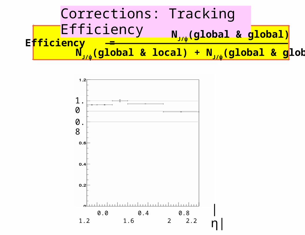
Corrections: Tracking Efficiency

1.0

0.8

0.0 0.4 0.8 1.2 1.6 2 2.2

NJ/ψ(global & global)

NJ/ψ(global & local) + N

J/ψ(global & global) Efficiency =

|η|

Corrections: Isolation and Silicon Hit Requirement

pt in GeV

| y()| < 1.8

From data – Monte Carlo predicts isolation requirement to be 100% efficient.

Isolation efficiency for signal