1

On the Performance of Practical Ultra-DenseNetworks: The Major and Minor Factors

Ming Ding‡, Member, IEEE, David Lopez-Perez†, Member, IEEE

Abstract—In this paper, we conduct performance evaluationfor Ultra-Dense Networks (UDNs), and identify which modellingfactors play major roles and minor roles. From our study, wedraw the following conclusions. First, there are 3 factors/modelsthat have a major impact on the performance of UDNs, and theyshould be considered when performing theoretical analyses: i) amulti-piece path loss model with line-of-sight (LoS) and non-line-of-sight (NLoS) transmissions; ii) a non-zero antenna height dif-ference between base stations (BSs) and user equipments (UEs);iii) a finite BS/UE density. Second, there are 4 factors/models thathave a minor impact on the performance of UDNs, i.e., changingthe results quantitatively but not qualitatively, and thus theirincorporation into theoretical analyses is less urgent: i) a generalmulti-path fading model based on Rician fading; ii) a correlatedshadow fading model; iii) a BS density dependent transmissionpower; iv) a deterministic BS/user density. Finally, there are3 factors/models for future study: i) a BS vertical antennapattern; ii) multi-antenna and/or multi-BS joint transmissions;iii) a non-uniform distribution of BSs. Our conclusions can guideresearchers to down-select the assumptions in their theoreticalanalyses, so as to avoid unnecessarily complicated results, whilestill capturing the fundamentals of UDNs in a meaningful way.

I. INTRODUCTION

Recent market forecasts predict that the mobile data trafficvolume density will keep growing towards 2030 and beyondthe so-called 1000× wireless capacity demand [1]. This in-crease is expected to be fuelled by the growth of mobilebroadband services, where high-quality videos, e.g., ultra-highdefinition and 4K resolution videos, are becoming an integralpart of today’s media contents. Moreover, new emergingservices such as machine type communications (MTC) andinternet of things (IoT) will contribute to the increase ofmassive data. This poses an ultimate challenge to the wirelessindustry, which must offer an exponentially increasing trafficin a profitable and energy efficient manner. To make thingseven more complex, the current economic situation aroundthe globe aggravates the pressure for mobile operators andvendors to stay competitive, rendering the decision on howto increase network capacity in a cost-effective manner evenmore critical.

Previous practice in the wireless industry shows that thewireless network capacity has increased around one millionfold from 1950 to 2000, in which an astounding 2700× gainwas achieved through network densification using smallercells [2]. In the first decade of 2000, network densification con-tinued to serve the 3rd Generation Partnership Project (3GPP)

‡Ming Ding is with Data61, CSIRO, Australia (e-mail:Ming.Ding@data61.csiro.au).

†David Lopez-Perez is with Nokia Bell Labs, Ireland (email: david.lopez-perez@nokia.com).

4th-generation (4G) Long Term Evolution (LTE) networks,and is expected to remain as one of the main forces to drivethe 5th-generation (5G) networks onward [2], [3]. Indeed, theorthogonal deployment1 of ultra-dense (UD) small cell net-works (SCNs), or simply ultra-dense networks (UDNs), withinthe existing macrocell network at sub-6 GHz frequencies2, isenvisaged as one of the workhorses for capacity enhancementin 5G, due to its large spatial reuse of spectrum and its easymanagement. The latter one arises from its low interactionwith the macrocell tier, e.g., no inter-tier interference [2].

The performance analysis of UDNs, however, is challengingbecause UDNs are fundamentally different from the current4G sparse/dense networks, and thus it is difficult to iden-tify the essential factors that have a key impact on UDNperformance. To elaborate on this, Table I provides a listof key factors/models/parameters related to the performanceanalysis of SCNs, along with their assumptions adopted inthe 3GPP. This list is far from exhaustive, but it includesthose assumptions that are essential in any SCN performanceevaluation campaign in the 3GPP [5], [6]. For clarity, theassumptions in Table I are classified into two categories, i.e.,network scenario (NS) and wireless system (WS).

More specifically,• The assumptions on the NS characterise the deployments

of base stations (BSs) and user equipments (UEs).• The assumptions on the WS characterise the channel

models and the transmit/receive capabilities.Considering the 10 factors listed in Table I, a straightfor-ward methodology to understand the fundamental differencesbetween UDNs and sparse/dense networks would be to in-vestigate the performance impact of those factors and theircombinations one by one, thus drawing useful conclusionson which factors should define the fundamental behavioursof UDNs. Since the 3GPP assumptions on those factors wereagreed upon by major companies in the wireless industry allover the world, the more of these assumptions an analysis canconsider, the more practical the analysis will be.

The theoretical community has already started to explorethis approach, and some of those assumptions in Table Ihave already been considered in various works to derive theperformance of UDNs, e.g., through stochastic geometry (SG)analyses. In more detail, in SG analyses, BS positions are

1Here, the orthogonal deployment means that small cells and macrocellsare operating on different frequency spectrum, i.e., 3GPP Small Cell Scenario#2a [3].

2In this paper, we focus on the spatial reuse gain of UDNs at sub-6 GHzfrequencies, and we do not consider millimeter wave communications, as suchtopic stands on its own and requires a completely new analysis [4].

2

Table IA LIST OF FACTORS FOR THE PERFORMANCE ANALYSIS OF UDNS.

Factorcategory

Factorindex Factor and its assumption in the 3GPP [5], [6] Assumption in our SG analysis

(Sections II and III)Assumption inour simulation

NetworkScenario

(NS)

NS 1 Finite BS and UE densities X X

NS 2 Deterministic BS and UE densities Random BS and UE numbers(Poisson-distributed) X [Focus of this paper]

NS 3 Non-uniform distribution of BSs with someconstraints on the minimum BS-to-BS distance

Unconstrained uniformdistribution of BSs

Unconstrained uniformdistribution of BSs

WirelessSystem(WS)

WS 1 Multi-piece path loss with LoS/NLoS transmissions X X

WS 2 3D BS-to-UE distance for path loss calculationconsidering BS/UE antenna heights X X

WS 3 Generalized Rician fading Rayleigh fading X [Focus of this paper]WS 4 Correlated shadow fading None X [Focus of this paper]WS 5 BS density dependent BS transmission power Constant BS transmission power X [Focus of this paper]WS 6 BS vertical antenna pattern None NoneWS 7 Multi-antenna and/or multi-BS joint transmissions None None

typically modelled as a Homogeneous Poisson Point Process(HPPP) on the plane, and closed-form expressions of coverageprobability can be found for some scenarios in single-tier cel-lular networks [7] and multi-tier cellular networks [8]. Usinga simple modelling, the major conclusion in [7], [8] is thatneither the number of cells nor the number of cell tiers changesthe coverage probability in interference-limited fully-loadedwireless networks. Recently, a few noteworthy studies havebeen carried out to revisit the network performance analysis ofUDNs under more practical assumptions [9]–[15]. These newstudies include the following assumptions in Table I: i) a multi-piece path loss model with line-of-sight (LoS) and non-line-of-sight (NLoS) transmissions (WS 1), ii) a non-zero antennaheight difference between BSs and UEs (WS 2), and iii) a finiteBS/UE density (NS 1). The inclusion of these assumptionssignificantly changed the previous conclusion, indicating thatthe coverage probability performance of UDNs is neither aconvex nor a concave function with respect to the BS density.

In light of such drastic change of conclusions, one may askthe following intriguing question: What if we further considermore assumptions in SG analyses? Will it qualitatively changethe recently obtained conclusions in [9]–[15]? In this paper,we will address this fundamental question by investigating theperformance impact of the 3GPP assumptions of WS 3, WS 4,WS 5 and NS 2 in Table I.

The rest of this paper is structured as follows:• Section II describes the network scenario and the wireless

system model used in our SG analysis, mostly recom-mended by the 3GPP.

• Section III presents our previous theoretical results interms of the coverage probability, and discusses ourmain results on the performance impact of the 3GPPassumptions of NS 1, WS 1 and WS 2 in Table I.

• Section IV describes in more detail the newly consid-ered assumptions addressed in this paper, i.e., the 3GPPassumptions of WS 3, WS 4, WS 5 and NS 2.

• Section V discloses our simulation results on the perfor-mance impact of these newly considered assumptions.

• Section VI provides some discussion on the performanceimpact of the remaining 3GPP assumptions of WS 6,

WS 7 and NS 3, which are left as our future work.• The conclusions are drawn in Section VII.

II. NETWORK SCENARIO AND WIRELESS SYSTEM MODEL

In this section, we present the network scenario and thewireless system model considered in this paper. Note that mostof our assumptions on cellular networks are in line with therecommendations by the 3GPP [5], [6].

A. Network Scenario

We consider a cellular network with BSs deployed on aplane according to a homogeneous Poisson point process(HPPP) Φ with a density of λBSs/km2. Active UEs are alsoPoisson distributed in the considered network with a densityof ρUEs/km2. We only consider active UEs in the networkbecause non-active UEs do not trigger data transmission, andthus they are ignored in our analysis. Note that the total UEnumber in cellular networks should be much higher than thenumber of the active UEs, but at a certain time slot and ona certain frequency band, the active UEs with data trafficdemands may not be too many. A typical density of the activeUEs in 5G should be around 300 UEs/km2 [2].

In practice, a BS should mute its transmission if thereis no UE connected to it, which reduces unnecessary inter-cell interference and energy consumption [15]. Since UEs arerandomly and uniformly distributed in the network, it can beassumed that the active BSs also follow an HPPP distributionΦ [16], the density of which is denoted by λBSs/km2. Notethat 0 ≤ λ ≤ λ, and a larger ρ leads to a larger λ. Details onthe computation of λ can be found in [15].

B. Wireless System Model

We denote by r the two-dimensional (2D) distance betweena BS and an a UE, and by L the absolute antenna height dif-ference between a BS and a UE. Hence, the three-dimensional(3D) distance between a BS and a UE can be expressed as

w =√r2 + L2, (1)

3

where L is in the order of several meters for the current 4Gnetworks. For example, according to the 3GPP assumptionsfor small cell networks, L equals to 8.5 m, as the BS antennaheight and the UE antenna height are assumed to be 10 m and1.5 m, respectively [17].

Following the 3GPP recommendations [5], [6], we considerpractical line-of-sight (LoS) and non-line-of-sight (NLoS)transmissions, and treat them as probabilistic events. Specifi-cally, we adopt a very general path loss model, in which thepath loss ζ (w) is segmented into N pieces, i.e.,

ζ (w) =

ζ1 (w) , when 0 ≤ w ≤ d1

ζ2 (w) , when d1 < w ≤ d2

......

ζN (w) , when w > dN−1

, (2)

where each piece ζn (w) , n ∈ {1, 2, . . . , N} is modelled as

ζn (w)=

{ζLn (w) = AL

nw−αL

n ,

ζNLn (w) = ANL

n w−αNLn ,

LoS Prob: PrLn (w)

NLoS Prob: 1− PrLn (w)

,

(3)where

• ζLn (w) and ζNL

n (w) , n ∈ {1, 2, . . . , N} are the n-th piecepath loss functions for the LoS transmission and theNLoS transmission, respectively,

• ALn and ANL

n are the path losses at a reference distancer = 1 for the LoS and the NLoS cases, respectively,

• αLn and αNL

n are the path loss exponents for the LoS andthe NLoS cases, respectively.

• In practice, ALn, ANL

n , αLn and αNL

n are constants obtain-able from field tests [5], [6].

• PrLn (w) is the n-th piece LoS probability function that

a transmitter and a receiver separated by a distance whas a LoS path, which is assumed to be a monotonicallydecreasing function with regard to w. Such assumptionhas been confirmed by [5], [6].

For convenience,{ζLn (w)

}and

{ζNLn (w)

}are further

stacked into piece-wise functions written as

ζPath (w) =

ζPath1 (w) , when 0 ≤ w ≤ d1

ζPath2 (w) , when d1 < w ≤ d2

......

ζPathN (w) , when w > dN−1

, (4)

where the string variable Path takes the value of “L” and“NL” for the LoS and the NLoS cases, respectively. Besides,{

PrLn (w)

}is also stacked into a piece-wise function as

PrL (w) =

PrL

1 (w) , when 0 ≤ w ≤ d1

PrL2 (w) , when d1 < w ≤ d2

......

PrLN (w) , when w > dN−1

. (5)

As a special case, in the following subsections, we considera two-piece path loss function and a LoS probability functiondefined by the 3GPP [5]. Specifically, we use the following

path loss function,

ζ (w) =

{ALw−α

L

,

ANLw−αNL

,

LoS Prob: PrL (w)

NLoS Prob: 1− PrL (w), (6)

together with the following LoS probability function,

PrL (w) =

{1− 5 exp (−R1/w) ,

5 exp (−w/R2) ,

0 < w ≤ d1

w > d1

, (7)

where R1 = 156 m, R2 = 30 m, and d1 = R1

ln 10 [5]. Thecombination of the path loss function in (6) and the LoSprobability function in (7) can be deemed as a special case ofthe proposed path loss model in (2) with the following sub-stitutions: N = 2, ζL

1 (w) = ζL2 (w) = ALw−α

L

, ζNL1 (w) =

ζNL2 (w) = ANLw−α

NL

, PrL1 (w) = 1 − 5 exp (−R1/w), and

PrL2 (w) = 5 exp (−w/R2). For clarity, this model is referred

to as the 3GPP Path Loss Model hereafter.Moreover, in this paper, we also assume a practical user

association strategy (UAS), in which each UE is connectedto the BS with the smallest path loss (i.e., with the largestζ (r)) to the UE [5], [6]. We also assume that each BS/UEis equipped with an isotropic antenna, and that the multi-pathfading between a BS and a UE is modelled as independentlyidentical distributed (i.i.d.) Rayleigh fading [9], [12]–[15].

III. DISCUSSION ON THE STATE-OF-THE-ART RESULTSON THE PERFORMANCE ANALYSIS OF UDNS

Using the theory of stochastic geometry (SG) and thepresented assumptions in previous subsections, we investigatedthe coverage probability performance of SCNs by consideringthe performance of a typical UE located at the origin o. Insuch studies [13]–[15], we analysed in detail the performanceimpact of the 3GPP assumptions of NS 1, WS 1 and WS 2 inTable I. The concept of coverage probability and a summaryof our results are presented in the following.

A. The Coverage Probability

The coverage probability is defined as the probability thatthe signal-to-interference-plus-noise ratio (SINR) of the typi-cal UE is above a designated threshold γ:

pcov (λ, γ) = Pr [SINR > γ] , (8)

where the SINR is computed by

SINR =Pζ (r)h

Iagg + PN, (9)

where h is the channel gain, which is modelled as an ex-ponentially distributed random variable (RV) with a mean ofone (due to our consideration on Rayleigh fading presentedbefore), P is the transmission power at each BS, PN is theadditive white Gaussian noise (AWGN) power at the typicalUE, and Iagg is the cumulative interference given by

Iagg =∑

i: bi∈Φ\bo

Pβigi, (10)

where bo is the BS serving the typical UE, bi is the i-thinterfering BS, βi is the path loss from bi to the typical UE,

4

Fig. 1. Theoretical performance comparison of the coverage probabilitywhen the SINR threshold γ = 0 dB. Note that all the results are obtainedusing the 3GPP Path Loss Model introduced in Subsection II-B. Moreover,the BS density regions for the 4G and 5G networks have been illustrated inthe figure, considering that the maximum BS density of the 4G SCNs is inthe order of 102 BSs/km2 [2], [3].

and gi is the multi-path fading channel gain associated withbi. Note that when all BSs are assumed to be active, the set ofall BSs Φ should be used in the expression of Iagg [9], [10],[12]–[14]. However, in our system model with idle mode at thesmall cell BSs and a finite UE density (see Subsection II-A),only the active BSs in Φ \ bo inject effective interference intothe network, where Φ denotes the set of the active BSs. Hence,the BSs in idle mode are not taken into account in the analysisof Iagg shown in (10), due to their muted transmissions.

B. Summary of Previous Findings

As a summary, to illustrate our findings in [13]–[15], weplot the SCN performance results in terms of the coverageprobability in Fig. 1.

The results in Fig. 1 are analytical ones validated bysimulations in [13]–[15]. Note that in Fig. 1, L denotes theabsolute antenna height difference between BSs and UEs. Asindicated in Subsection II-B, L = 8.5 m in the current 3GPPassumption for small cell scenarios, while L = 0 m is afuturistic assumption where BS antennas are installed at theUE height. Besides, the other parameters used to obtain theresults in Fig. 1 are αL = 2.09, αNL = 3.75, AL = 10−10.38,ANL = 10−14.54, P = 24 dBm, PN = −95 dBm [5].

From Fig. 1, we can draw the following observations:• Performance impact of WS 1: The curve with plus markers

represents the results in [13], where we consider the3GPP multi-piece path loss function with LoS/NLoStransmissions [5] and ignore the 3GPP assumptions ofWS 2 and NS 2, i.e., setting L = 0 m and deploying aninfinite number of UEs. From those results, it can be seenthat when the BS density is larger than a threshold around102 BSs/km2, the coverage probability will continuouslydecrease as the SCN becomes denser. This is becauseUDNs imply high probabilities of LoS transmissionsbetween BSs and UEs, which leads to a performancedegradation caused by a faster growth of the interference

power compared with the signal power [13]. This is dueto the transition of a large number of interference pathsfrom NLoS (usually with a large path loss exponent αNL)to LoS (usually with a small path loss exponent αL).

• Performance impact of WS 2: The curve with squaremarkers represents the results in [14], where we considerthe 3GPP assumptions of multi-piece path loss functionwith LoS/NLoS transmissions and L = 8.5 m [5], whilestill keeping the assumption of an infinite number ofUEs. From those results, it can be seen that the coverageprobability shows a concerning trajectory toward zerowhen the BS density is larger than 103 BSs/km2. Thisis because UDNs make the antenna height differencebetween BSs and UEs non-negligible, which gives riseto another performance degradation due to a cap onthe signal power, resulted from the bounded minimumdistance between a UE and its serving BS [14].

• Performance impact of NS 2: The curves with circle andtriangle markers represents the results in [15], wherewe consider the 3GPP assumptions of multi-piece pathloss function with LoS/NLoS transmissions and a finiteUE density of 300 UEs/km2 (a typical UE density in5G [2]). Moreover, both the assumptions of L = 0 m andL = 8.5 m are investigated in Fig. 1. As we can observe,when the BS density surpasses the UE density, i.e.,300 BSs/km2, thus creating a surplus of BSs, the coverageprobability will continuously increase. Such performancebehaviour of the coverage probability increasing in UDNsis referred to as the Coverage Probability Takeoff in [15].The intuition behind the Coverage Probability Takeoff isthat UDNs provide a surplus of BSs with respect to UEs,which provide a performance improvement, thanks to theBS diversity gain and the BS idle mode operation. Inmore detail, as discussed in II-A, since the UE densityis finite in practical networks, a large number of BSscould switch off their transmission modules in a UDN,thus enter idle modes, if there is no active UE withintheir coverage areas. This helps to mitigate unnecessaryinter-cell interference and reduce energy consumption.

IV. DISCUSSION ON THE INCORPORATION OF MORE 3GPPASSUMPTIONS INTO THE MODELING

To investigate whether the previous conclusions still hold inmore practical network scenarios, additional assumptions [5],[6] will also be considered in our analysis through simulations.The results will be discussed in Section V. Such additionalpractical assumptions are the 3GPP assumptions of WS 3,WS 4, WS 5 and NS 2 in Table I, which are presented in thesequel. Note that the authors of [11] have recently proposed anew approach of network performance analysis based on HPPPintensity matching, which facilitates the theoretical study ofsome of these additional 3GPP assumptions.

A. A general multi-path fading model based on Rician fading(WS 3 in Table I)

In SG analyses, the multi-path fading is usually modelledas Rayleigh fading for simplicity. However, in the 3GPP, a

5

more practical model based on generalised Rician fading iswidely adopted [6]. Hence, we consider the practical multi-path Rician fading model defined in the 3GPP [6], where theK factor in dB scale (the ratio between the power in the directpath and the power in the other scattered paths) is modelledas K[dB] = 13− 0.03w, where w is defined in (1).

B. A correlated shadow fading model (WS 4 in Table I)

In SG analyses, the shadow fading is usually not consideredor simply modelled as independently identical distributed(i.i.d.) RVs. However, in the 3GPP, a more practical corre-lated shadow fading is often used [5], [6], [18]. Hence, weconsider the practical correlated shadow fading model definedin 3GPP [5], where the shadow fading in dB is modelled aszero-mean Gaussian a random variable, e.g., with a standarddeviation of 10 dB [5]. The correlation coefficient betweenthe shadow fading values associated with two different BSsis denoted by τ , where τ = 0.5 in [5].

C. A BS density dependent BS transmission power (WS 5 inTable I)

In SG analyses, the BS transmission power is usuallyassumed to be a constant. However, in the 3GPP, it is generallyagreed that the BS transmission power should decrease as theSCN densifies because the per-cell coverage area shrinks [5].Hence, we embrace the practical self-organising BS transmis-sion power framework presented in [2], in which P varieswith the BS density λ. Specifically, the transmit power of eachBS is configured such that it provides a signal-to-noise-ratio(SNR) of η0 = 15 dB at the edge of the average coveragearea for a UE with NLoS transmissions. The distance froma cell-edge UE to its serving BS with an average coveragearea is calculated by r0 =

√1λπ , which is the radius of an

equivalent disk-shaped coverage area with an area size of 1λ .

Therefore, the worst-case path loss is given by ANLr−αNL

0 andthe required transmission power to enable a η0 dB SNR in thiscase can be computed as [2]

P (λ) =10

η010 PN

ANLr−αNL

0

. (11)

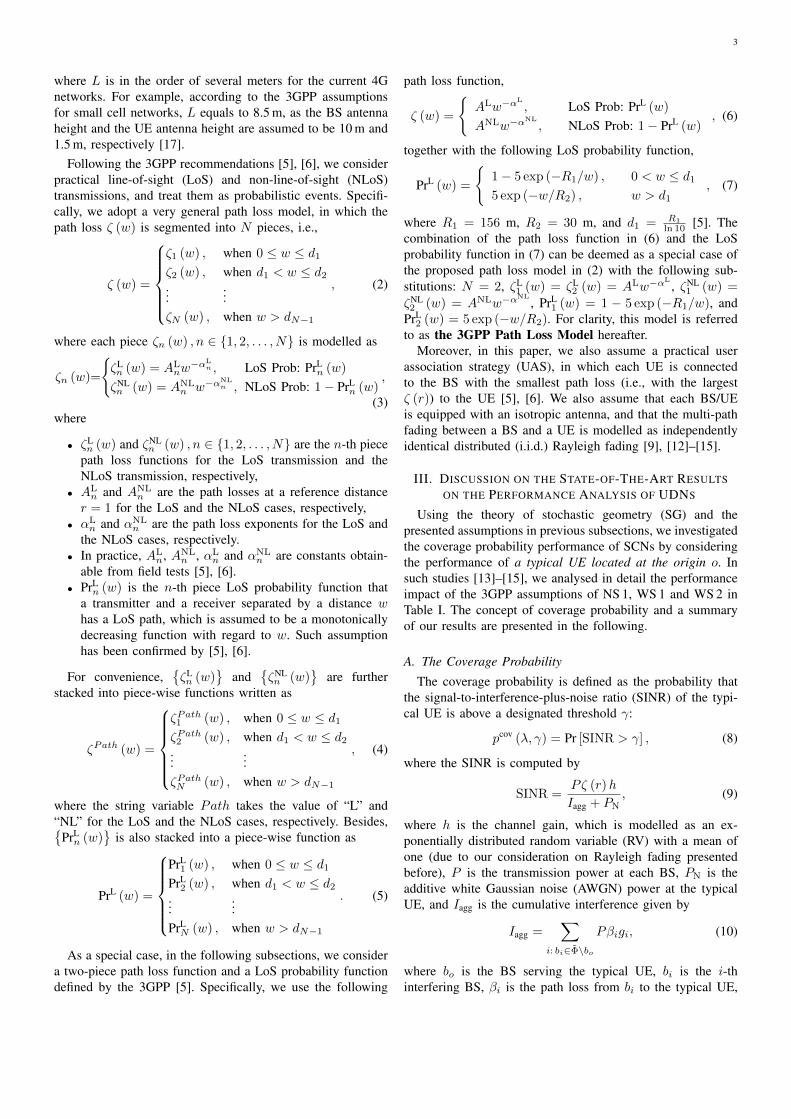
In Fig. 2, we plot the BS density dependent transmissionpower in dBm to illustrate this realistic power configurationwhen η0 = 15 dB. Note that our modelling of P is practical,covering the cases of macrocells and picocells recommendedin the LTE networks. More specifically, the typical BS densi-ties of LTE macrocells and picocells are respectively severalBSs/km2 and around 50 BSs/km2 [17], respectively. As aresult, the typical P of macrocell BSs and picocells BSs arerespectively assumed to be 46 dBm and 24 dBm in the 3GPPstandards [17], which match well with our modelling.

D. A deterministic BS/UE density (NS 2 in Table I)

In SG analyses, the BS/UE number is usually modelledas a Poisson distributed random variable (RV). However, inthe 3GPP, a deterministic BS/UE number is commonly used

Fig. 2. The BS density dependent transmission power in dBm.

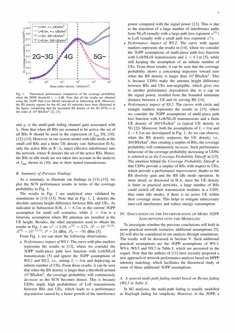
Fig. 3. Simulated performance comparison of the coverage probability withmore 3GPP assumptions when the SINR threshold γ = 0 dB.

for a given BS/UE density [5]. Hence, we use deterministicdensities λBSs/km2 and ρUEs/km2 to characterize the BSand UE deployments, respectively, instead of modelling theirnumbers as Poisson distributed RVs.

V. MAIN RESULTS ON THE PERFORMANCE IMPACT OF THEADDITIONAL 3GPP ASSUMPTIONS

On top of the 3GPP assumptions discussed in Subsec-tion III-B, in this section, we consider the 4 additional3GPP assumptions described in Section IV, and study theirperformance impacts on UDNs. More specifically, using thesame parameter values for Fig. 1, we conduct simulationsto investigate the coverage probability performance of SCNswhile also considering the 3GPP assumptions of WS 3, WS 4,WS 5 and NS 2 in Table I. The results are plotted in Fig. 3.

Comparing Fig. 1 with Fig. 3, we can draw the followingobservations:• Those 4 additional 3GPP assumptions introduced in Sec-

tion IV do not change the fundamental behaviours ofUDNs shown in Fig. 1, i.e.,

– the performance degradation due to the transition ofa large number of interfering links from NLoS to

6

LoS, when λ ∈[102, 103

]BSs/km2,

– the further performance degradation, due to the capon the signal power caused by the non-zero antennaheight difference between BSs and UEs, when L =8.5 m and λ is larger than 103 BSs/km2, and

– the performance improvement when λ is larger thanρ, thus creating a surplus of BSs and thus allowingfor idle mode operation to mitigate unnecessaryinter-cell interference.

• The performance behaviour of sparse networks (λ ∈[10−1, 100

]BSs/km2) is different in Fig. 3 compared

with that in Fig. 1. This is mainly due to the larger BStransmission power used in Fig. 3 for sparse networks, asdisplayed in Fig. 2, which is helpful to remove coverageholes in the noise-limited region. Based on our knowledgeof the successful operation of the existing 2G/3G systems,the results in Fig. 3 make more sense than those inFig. 1, since the macrocell BS transmission power inthe 2G/3G systems is indeed much larger than 24 dBm,which is the case for Fig. 1. Nevertheless, such BSdensity dependent transmission power has a minor impacton UDNs, because BSs in UDNs usually work in ainterference-limited region, and thus the BS transmissionpower in the signal power and that in the aggregatedinterference power cancel out each other. This is obviousfrom the SINR expression in (9).

VI. FUTURE WORK

The performance impact of the remaining 3 assumptions inTable I, i.e., the 3GPP assumptions of WS 6, WS 7 and NS 3,are left to our future work, but presented in the following:• A 3D antenna pattern: In SG analyses, the vertical an-

tenna pattern at each BS is usually ignored for simplicity.However, in the 3GPP performance evaluations, it is ofgood practice to consider 3D antenna patterns, wherethe main beam is mechanically and/or electrically tilteddownwards to improve the signal power as well as toreduce the inter-cell interference [5], [6].

• A Multi-antenna and/or multi-BS joint transmissionframework: In SG analyses, each BS/UE is usuallyequipped with one omni-directional antenna for simplic-ity. However, in the 3GPP performance evaluations, it isusual to consider multi-antenna transmissions [5], evenwith an enhancement of multi-BS cooperation [19]–[21].

• A non-uniform distribution of BSs with some constraintson the minimum BS-to-BS distance: In SG analyses, BSsare usually assumed to be uniformly deployed in the in-terested network area. However, in the 3GPP performanceevaluations, small cell clusters are often considered, andit is forbidden to place any two BSs too close to eachother [5]. Such assumption is in line with the realisticnetwork planning to avoid strong inter-cell interference.It is interesting to note that several recent studies arelooking at this aspect from difference angles [22]–[24].In particular, a deterministic hexagonal grid networkmodel [7] might be useful for the analysis. More specif-ically, we can construct an idealistic BS deployment on

Fig. 4. Illustration of the ideal BS deployment in a hexagonal grid network.

a perfect hexagonal lattice, and then we can perform anetwork analysis on such BS deployment to extract anupper-bound of the SINR performance. Note that the BSdeployment on a hexagonal lattice leads to an upper-bound performance because BSs are evenly distributed inthe network scenario, and thus very strong interferencedue to close proximity is precluded in the analysis [7].Illustration of such hexagonal grid network is providedin Fig. 4.

Finally, it is very important to point out that even if ananalysis can treat all the assumptions in Table I, a non-negligible gap may still exist between the analytical resultsand the performance results in reality, because of the followingnon-tractable factors [5]:• non-full-buffer traffic• non-linear channel measurement errors• imperfect channel state information (CSI)• hybrid automatic repeat request (HARQ) processes• UE misreading of control signalling• discrete modulation and coding schemes• UE mobility and handover procedures, and so on.Hence, in the context of the performance analysis for

UDNs, a high priority should be given to identifying theperformance trends qualitatively, rather than improvingthe numerical results quantitatively.

VII. CONCLUSION

In this paper, we have conducted a performance evaluationof UDNs, and identified which modelling factors really matterin theoretical analyses. From our study, we have identified that3 factors/models have a major impact on the performanceof UDNs, and they should be considered when performingtheoretical analyses:• a multi-piece path loss model with LoS/NLoS transmis-

sions;• a non-zero antenna height difference between BSs and

UEs;

7

• a finite BS/UE density.In contrast, we have found that the following 4 fac-

tors/models have a minor impact on the performance ofUDNs, i.e., change the results quantitatively but not qualita-tively, and thus their incorporation into theoretical analyses isless urgent:• a general multi-path fading model based on Rician fading;• a correlated shadow fading model;• a BS density dependent transmission power;• a deterministic BS/user density.Finally, there are 3 factors/models for future study:• a BS vertical antenna pattern;• multi-antenna and/or multi-BS joint transmissions;• a non-uniform distribution of BSs.Our conclusions can guide researchers to down-select the

assumptions in their theoretical analyses, so as to avoidunnecessarily complicated results, while still capturing thefundamentals of UDNs in a meaningful way.

REFERENCES

[1] CISCO, “Cisco visual networking index: Global mobile data trafficforecast update (2015-2020),” Feb. 2016.

[2] D. López-Pérez, M. Ding, H. Claussen, and A. Jafari, “Towards 1Gbps/UE in cellular systems: Understanding ultra-dense small celldeployments,” IEEE Communications Surveys Tutorials, vol. 17, no. 4,pp. 2078–2101, Jun. 2015.

[3] 3GPP, “TR 36.872: Small cell enhancements for E-UTRA and E-UTRAN - Physical layer aspects,” Dec. 2013.

[4] S. Rangan, T. S. Rappaport, and E. Erkip, “Millimeter-wave cellularwireless networks: Potentials and challenges,” Proceedings of the IEEE,vol. 102, no. 3, pp. 366–385, Mar. 2014.

[5] 3GPP, “TR 36.828: Further enhancements to LTE Time Division Duplexfor Downlink-Uplink interference management and traffic adaptation,”Jun. 2012.

[6] Spatial Channel Model AHG, “Subsection 3.5.3, Spatial Channel ModelText Description V6.0,” Apr. 2003.

[7] J. Andrews, F. Baccelli, and R. Ganti, “A tractable approach to coverageand rate in cellular networks,” IEEE Transactions on Communications,vol. 59, no. 11, pp. 3122–3134, Nov. 2011.

[8] H. S. Dhillon, R. K. Ganti, F. Baccelli, and J. G. Andrews, “Modelingand analysis of K-tier downlink heterogeneous cellular networks,” IEEEJournal on Selected Areas in Communications, vol. 30, no. 3, pp. 550–560, Apr. 2012.

[9] X. Zhang and J. Andrews, “Downlink cellular network analysis withmulti-slope path loss models,” IEEE Transactions on Communications,vol. 63, no. 5, pp. 1881–1894, May 2015.

[10] T. Bai and R. Heath, “Coverage and rate analysis for millimeter-wavecellular networks,” IEEE Transactions on Wireless Communications,vol. 14, no. 2, pp. 1100–1114, Feb. 2015.

[11] M. D. Renzo, W. Lu, and P. Guan, “The intensity matching approach:A tractable stochastic geometry approximation to system-level analysisof cellular networks,” IEEE Transactions on Wireless Communications,vol. 15, no. 9, pp. 5963–5983, Sep. 2016.

[12] M. Ding, D. López-Pérez, G. Mao, P. Wang, and Z. Lin, “Will the areaspectral efficiency monotonically grow as small cells go dense?” IEEEGLOBECOM 2015, pp. 1–7, Dec. 2015.

[13] M. Ding, P. Wang, D. López-Pérez, G. Mao, and Z. Lin, “Performanceimpact of LoS and NLoS transmissions in dense cellular networks,”IEEE Transactions on Wireless Communications, vol. 15, no. 3, pp.2365–2380, Mar. 2016.

[14] M. Ding and D. Lopez Perez, “Please Lower Small Cell Antenna Heightsin 5G,” arXiv:1611.01869 [cs.IT], to appear in IEEE Globecom 2016,Nov. 2016.

[15] M. Ding, D. Lopez Perez, G. Mao, and Z. Lin, “Study on the idle modecapability with LoS and NLoS transmissions,” IEEE Globecom 2016,pp. 1–6, Dec. 2016.

[16] S. Lee and K. Huang, “Coverage and economy of cellular networks withmany base stations,” IEEE Communications Letters, vol. 16, no. 7, pp.1038–1040, Jul. 2012.

[17] 3GPP, “TR 36.814: Further advancements for E-UTRA physical layeraspects,” Mar. 2010.

[18] M. Ding, M. Zhang, D. López-Pérez, and H. Claussen, “Correlatedshadow fading for cellular network system-level simulations with wrap-around,” 2015 IEEE International Conference on Communications(ICC), pp. 2245–2250, Jun. 2015.

[19] M. Ding, M. Zhang, H. Luo, and W. Chen, “Leakage-based robust beam-forming for multi-antenna broadcast system with per-antenna powerconstraints and quantized cdi,” IEEE Transactions on Signal Processing,vol. 61, no. 21, pp. 5181–5192, Nov. 2013.

[20] M. Ding, J. Zou, Z. Yang, H. Luo, and W. Chen, “Sequential and in-cremental precoder design for joint transmission network mimo systemswith imperfect backhaul,” IEEE Transactions on Vehicular Technology,vol. 61, no. 6, pp. 2490–2503, Jul. 2012.

[21] M. Ding and H. Luo, Multi-point Cooperative Communication Systems:Theory and Applications. Springer, 2013.

[22] A. Al-Hourani, R. J. Evans, and K. Sithamparanathan, “Near-est neighbour distance distribution in hard-core point processes,”arXiv:1606.03695 [cs.IT], Jun. 2016.

[23] C. Choi, J. O. Woo, and J. G. Andrews, “Modeling a spatially correlatedcellular network with strong repulsion,” arXiv:1701.02261 [cs.IT], Jan.2017.

[24] M. Ding, D. López-Pérez, G. Mao, and Z. Lin, “Microscopic analysisof the uplink interference in FDMA small cell networks,” IEEE Trans.on Wireless Communications, vol. 15, no. 6, pp. 4277–4291, Jun. 2016.