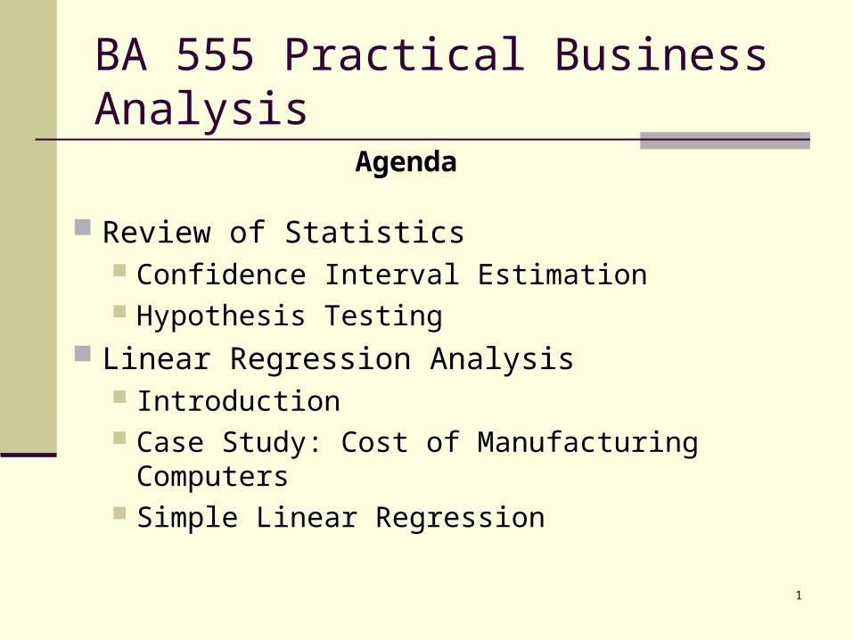
1

BA 555 Practical Business Analysis

Review of Statistics Confidence Interval Estimation Hypothesis Testing

Linear Regression Analysis Introduction Case Study: Cost of Manufacturing Computers Simple Linear Regression

Agenda

2

The Empirical Rule (p.5)

1. Approximately 68% of the observations will fall within 1 standard deviation of the mean. 2. Approximately 95% of the observations will fall within 2 standard deviations of the mean. 3. Approximately 99.7% of the observations will fall within 3 standard deviations of the mean.

3

3

3

sx

2

2

2

sx

1sx

3

3

3

sx

2

2

2

sx

1

sx

0

x

0.15% 2.35% 13.5% 34% 34% 13.5% 2.35% 0.15%

68%

95%

99.7%

3

3

3

sx

2

2

2

sx

1sx

3

3

3

sx

2

2

2

sx

1

sx

0

x

0.15% 2.35% 13.5% 34% 34% 13.5% 2.35% 0.15%

68%

95%

99.7%

3

Review Example

Suppose that the average hourly earnings of production workers over the past three years were reported to be $12.27, $12.85, and $13.39 with the

standard deviations $0.15, $0.18, and $0.23, respectively. The average hourly earnings of the production

workers in your company also continued to rise over the past three years from $12.72 in 2002, $13.35 in 2003, to $13.95 in 2004.

Assume that the distribution of the hourly earnings for all production workers is mound-shaped.

Do the earnings in your company become less and less competitive? Why or why not.

4

Review Example

YearIndustry average

Industry

std.%

increaseCompany average

% increase

Z score

2002 12.27 0.15 12.72 3

2003 12.85 0.18 4.73% 13.35 4.95% 2.77

2004 13.39 0.23 4.20% 13.95 4.50% 2.43

5

The Empirical Rule

Generalize the results from the empirical rule. Justify the use of the mound-shaped

distribution.

3

3

3

sx

2

2

2

sx

1sx

3

3

3

sx

2

2

2

sx

1

sx

0

x

0.15% 2.35% 13.5% 34% 34% 13.5% 2.35% 0.15%

68%

95%

99.7%

6

Sampling Distribution (p.6)

The sampling distribution of a statistic is the probability distribution for all possible values of the statistic that results when random samples of size n are repeatedly drawn from the population.

When the sample size is large, what is the sampling distribution of the sample mean / sample proportion / the difference of two samples means / the difference of two sample proportions? NORMAL !!!

7

Central Limit Theorem (CLT) (p.6)

If X ~ N(, 2), then X ~ N( X

,nX

22 )

:::::::

,,, :4 Sample

,,, :3 Sample

,,, :2 Sample

,,, :1 Sample

444241

333231

222221

111211

XXXX

XXXX

XXXX

XXXX

n

n

n

n

8

Central Limit Theorem (CLT) (p.6)

If X ~ Any distribution with the mean , and variance 2, then X ~ N(

X,

nX

22 ) for large n.

:::::::

,,, :4 Sample

,,, :3 Sample

,,, :2 Sample

,,, :1 Sample

444241

333231

222221

111211

XXXX

XXXX

XXXX

XXXX

n

n

n

n

9

Summary: Sampling Distributions

The sampling distribution of a sample mean The sampling distribution of a sample

proportion The sampling distribution of the difference

between two sample means The sampling distribution of the difference

between two sample proportions

10

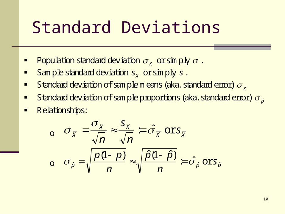
Standard Deviations

Population standard deviation X or simply .

Sample standard deviation Xs or simply s .

Standard deviation of sample means (aka. standard error) X

Standard deviation of sample proportions (aka. standard error) p

Relationships:

o XXXX

Xs

n

s

nor ˆ:

o ppp sn

pp

n

ppˆˆˆ or ˆ:

)ˆ1(ˆ)1(

11

Statistical Inference: Estimation

Research Question: What is the parameter value?

Sample of size n

Population

Tools (i.e., formulas):Point EstimatorInterval Estimator

12

Confidence Interval Estimation (p.7)

13

Example 1: Estimation for the population mean A random sampling of a company’s weekly

operating expenses for a sample of 48 weeks produced a sample mean of $5474 and a standard deviation of $764. Construct a 95% confidence interval for the company’s mean weekly expenses.

Example 2: Estimation for the population proportion

14

Statistical Inference: Hypothesis Testing

Research Question: Is the claim supported?

Sample of size n

Population

Tools (i.e., formulas):z or t statistic

15

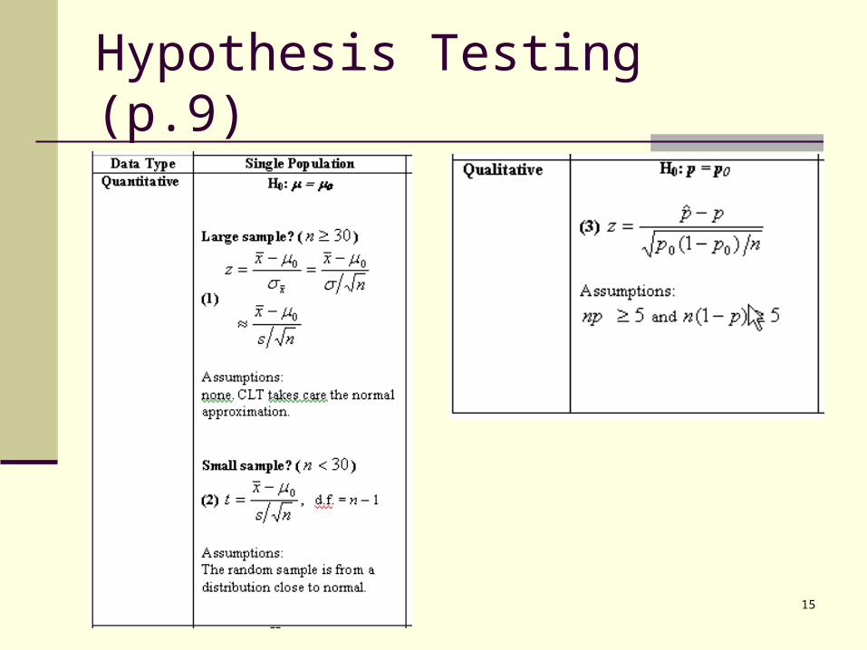
Hypothesis Testing (p.9)

16

Example

A bank has set up a customer service goal that the mean waiting time for its customers will be less than 2 minutes. The bank randomly samples 30 customers and finds that the sample mean is 100 seconds. Assuming that the sample is from a normal distribution and the standard deviation is 28 seconds, can the bank safely conclude that the population mean waiting time is less than 2 minutes?

17

Setting Up the Rejection RegionType I Error If we reject H0 (accept Ha) when in fact H0 is

true, this is a Type I error. False Alarm.

18

The P-Value of a Test (p.11)

The p-value or observed significance level is the smallest value of for which test results are statistically significant.

“the conclusion of rejecting H0 can be reached.”

19

Regression Analysis

A technique to examine the relationship between an outcome variable (dependent variable, Y) and a group of explanatory variables (independent variables, X1, X2, … Xk).

The model allows us to understand (quantify) the effect of each X on Y.

It also allows us to predict Y based on X1, X2, …. Xk.

20

Types of Relationship

Linear Relationship Simple Linear Relationship

Y = 0 + 1 X + Multiple Linear Relationship

Y = 0 + 1 X1 + 2 X2 + … + k Xk +

Nonlinear Relationship Y = 0 exp(1X+ Y = 0 + 1 X1 + 2 X1

2 + … etc.

Will focus only on linear relationship.

21

Simple Linear Regression Model

XY 10

population

sample

XY 10ˆˆˆ

True effect of X on Y

Estimated effect of X on Y

Key questions:1. Does X have any effect on Y?2. If yes, how large is the effect?3. Given X, what is the estimated Y?

22

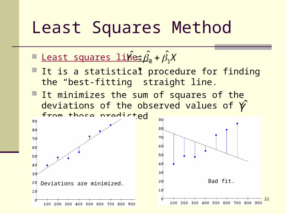
Least Squares Method

Least squares line: It is a statistical procedure for finding the “best-

fitting” straight line. It minimizes the sum of squares of the deviations of

the observed values of Y from those predicted Y

XY 10ˆˆˆ

Deviations are minimized. Bad fit.

23

Case: Cost of Manufacturing Computers (pp.13 – 45) A manufacturer produces computers. The goal is to

quantify cost drivers and to understand the variation in production costs from week to week.

The following production variables were recorded: COST: the total weekly production cost (in $millions) UNITS: the total number of units (in 000s) produced

during the week. LABOR: the total weekly direct labor cost (in $10K). SWITCH: the total number of times that the production

process was re-configured for different types of computers

FACTA: = 1 if the observation is from factory A; = 0 if from factory B.

24

Raw Data (p. 14)

Case FactA Units Switch Labor Cost(1000) (10,000) (million)

1 1 1.104 8 5.591181 1.1554562 0 1.044 12 6.836490 1.1441983 1 1.020 12 5.906357 1.1414904 1 0.986 6 5.050069 1.1196565 1 0.972 13 4.790412 1.1248156 0 1.005 11 5.474329 1.1373397 0 0.953 10 5.614134 1.1212758 0 1.083 9 6.002122 1.1532249 1 0.978 9 5.971627 1.119525

10 0 0.993 12 5.679461 1.13463511 1 0.958 12 4.320123 1.11938612 1 0.945 13 5.884950 1.11354313 1 1.012 7 4.593554 1.13212414 0 0.974 10 4.915151 1.13123815 1 0.910 11 4.969754 1.10497616 0 1.086 7 5.722599 1.15154717 0 0.962 11 6.109507 1.12747818 1 0.941 10 5.006398 1.11405819 0 1.046 9 6.141096 1.14087220 1 0.955 11 5.019560 1.11129021 1 1.096 12 5.741166 1.15904422 1 1.004 9 4.990734 1.12780523 0 0.997 8 4.662818 1.13066124 1 0.967 13 6.150249 1.12707325 1 1.068 6 6.038454 1.14104126 1 1.041 11 4.988593 1.14031927 1 0.989 16 6.104960 1.13017228 0 1.001 10 4.605764 1.13511829 1 1.008 9 5.529746 1.12132630 1 1.001 7 4.941728 1.12428431 1 0.984 10 6.456427 1.11501632 1 0.981 12 7.058013 1.12435333 1 0.944 11 4.626091 1.11631834 0 0.967 10 4.054482 1.12851735 0 1.018 9 5.820684 1.15023836 1 0.902 9 4.932339 1.09406137 0 1.049 11 5.798058 1.14379338 0 1.024 11 5.528302 1.14513539 1 1.044 7 6.635490 1.14215640 0 1.018 9 5.617445 1.14028541 0 0.937 11 5.275923 1.11441842 0 0.942 9 2.927715 1.11577443 0 1.061 11 6.750682 1.15406944 0 0.901 7 5.029670 1.10533545 0 1.078 9 7.005407 1.15336746 0 1.030 10 4.885713 1.14693447 0 0.981 8 6.362366 1.13042348 1 1.011 10 6.261692 1.13092949 1 1.016 9 5.677634 1.13634950 0 1.008 9 6.630767 1.14061651 0 1.059 11 6.930117 1.154121

1 1 1.104 8 5.591181 1.1554562 0 1.044 12 6.836490 1.1441983 1 1.020 12 5.906357 1.1414904 1 0.986 6 5.050069 1.1196565 1 0.972 13 4.790412 1.1248156 0 1.005 11 5.474329 1.1373397 0 0.953 10 5.614134 1.1212758 0 1.083 9 6.002122 1.1532249 1 0.978 9 5.971627 1.119525

10 0 0.993 12 5.679461 1.13463511 1 0.958 12 4.320123 1.11938612 1 0.945 13 5.884950 1.11354313 1 1.012 7 4.593554 1.13212414 0 0.974 10 4.915151 1.13123815 1 0.910 11 4.969754 1.10497616 0 1.086 7 5.722599 1.15154717 0 0.962 11 6.109507 1.12747818 1 0.941 10 5.006398 1.11405819 0 1.046 9 6.141096 1.14087220 1 0.955 11 5.019560 1.11129021 1 1.096 12 5.741166 1.15904422 1 1.004 9 4.990734 1.12780523 0 0.997 8 4.662818 1.13066124 1 0.967 13 6.150249 1.12707325 1 1.068 6 6.038454 1.14104126 1 1.041 11 4.988593 1.14031927 1 0.989 16 6.104960 1.13017228 0 1.001 10 4.605764 1.13511829 1 1.008 9 5.529746 1.12132630 1 1.001 7 4.941728 1.12428431 1 0.984 10 6.456427 1.11501632 1 0.981 12 7.058013 1.12435333 1 0.944 11 4.626091 1.11631834 0 0.967 10 4.054482 1.12851735 0 1.018 9 5.820684 1.15023836 1 0.902 9 4.932339 1.09406137 0 1.049 11 5.798058 1.14379338 0 1.024 11 5.528302 1.14513539 1 1.044 7 6.635490 1.14215640 0 1.018 9 5.617445 1.14028541 0 0.937 11 5.275923 1.11441842 0 0.942 9 2.927715 1.11577443 0 1.061 11 6.750682 1.15406944 0 0.901 7 5.029670 1.10533545 0 1.078 9 7.005407 1.15336746 0 1.030 10 4.885713 1.14693447 0 0.981 8 6.362366 1.13042348 1 1.011 10 6.261692 1.13092949 1 1.016 9 5.677634 1.13634950 0 1.008 9 6.630767 1.14061651 0 1.059 11 6.930117 1.15412152 0 1.019 13 6.415978 1.142435

How many possible regression models can we build?

25

Simple Linear Regression Model (pp. 17 – 26) Question1: Is Labor a significant cost driver?

This question leads us to think about the following model: Cost = f(Labor) + . Specifically, Cost = 0 + 1 Labor +

Question 2: How well does this model perform? (How accurate can Labor predict Cost?) This question leads us to try other regression

models and make comparison.

26

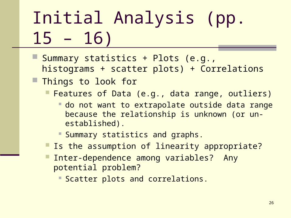
Initial Analysis (pp. 15 – 16)

Summary statistics + Plots (e.g., histograms + scatter plots) + Correlations

Things to look for Features of Data (e.g., data range, outliers)

do not want to extrapolate outside data range because the relationship is unknown (or un-established).

Summary statistics and graphs. Is the assumption of linearity appropriate? Inter-dependence among variables? Any potential

problem? Scatter plots and correlations.

27

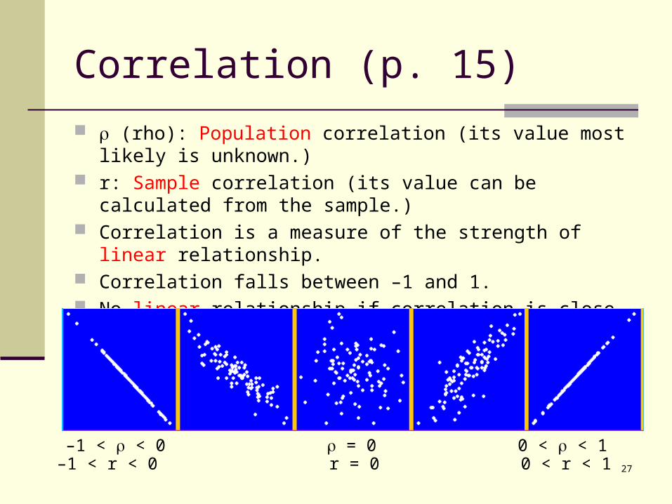
Correlation (p. 15)

(rho): Population correlation (its value most likely is unknown.) r: Sample correlation (its value can be calculated from the

sample.) Correlation is a measure of the strength of linear relationship. Correlation falls between –1 and 1. No linear relationship if correlation is close to 0. But, ….

= –1 –1 < < 0 = 0 0 < < 1 = 1r = –1 –1 < r < 0 r = 0 0 < r < 1 r = 1

28

Correlation (p. 15)

Cost Units Switch Labor Cost 0.9297 -0.0232 0.4520 ( 52) ( 52) ( 52) 0.0000 0.8706 0.0008 Units 0.9297 -0.1658 0.4603 ( 52) ( 52) ( 52) 0.0000 0.2402 0.0006 Switch -0.0232 -0.1658 0.1554 ( 52) ( 52) ( 52) 0.8706 0.2402 0.2714 Labor 0.4520 0.4603 0.1554 ( 52) ( 52) ( 52) 0.0008 0.0006 0.2714

Is 0.9297 a or r?

Sample size

P-value for

H0: = 0Ha: ≠ 0

29

Regression Analysis - Linear model: Y = a + b*X Dependent variable: Cost Independent variable: Labor Standard T Parameter Estimate Error Statistic P-Value

Intercept 1.08673 0.0127489 85.2409 0.0000 Slope 0.00810182 0.00226123 3.58293 0.0008 Analysis of Variance Source Sum of Squares Df Mean Square F-Ratio P-Value Model 0.00231465 1 0.00231465 12.84 0.0008 Residual 0.00901526 50 0.000180305 Total (Corr.) 0.0113299 51

Fitted Model (Least Squares Line) (p.18)

Error Standard

0-Estimate Statistic T

H0: 1 = 0Ha: 1 ≠ 0

1 or b1?0 or b0?

Sb1

Sb0b1b0

Degrees of freedom = n – k – 1, where n = sample size, k = # of Xs.

** Divide the p-value by 2for one-sided test. Makesure there is at least weakevidence for doing this step.

XY 0081.008673.1ˆ

30

Regression Analysis - Linear model: Y = a + b*X Dependent variable: Cost Independent variable: Labor Standard T Parameter Estimate Error Statistic P-Value

Intercept 1.08673 0.0127489 85.2409 0.0000 Slope 0.00810182 0.00226123 3.58293 0.0008 Analysis of Variance Source Sum of Squares Df Mean Square F-Ratio P-Value Model 0.00231465 1 0.00231465 12.84 0.0008 Residual 0.00901526 50 0.000180305 Total (Corr.) 0.0113299 51

Hypothesis Testing and Confidence Interval Estimation for (pp. 19 – 20)

Sb1 Sb0b1b0

Degrees of freedom = n – k – 1k = # of independent variables

Q1: Does Labor have any impact on Cost → Hypothesis TestingQ2: If so, how large is the impact? → Confidence Interval Estimation

31

Analysis of Variance (p. 21) Analysis of Variance Source Sum of Squares Df Mean Square F-Ratio P-Value

Model 0.00231465 1 0.00231465 12.84 0.0008 Residual 0.00901526 50 0.000180305 Total (Corr.) 0.0113299 51

Syy = SS Total =

2

1

)( yyn

ii 0.0113299.

SSR =SS of Regression Model =

2

1

)ˆ( yyn

ii 0.00231465.

SSE = SS of Error =

2

1

)ˆ( i

n

ii yy 0.00901526.

SS Total = SS Model + SS Error.

- Not very useful in simple regression.- Useful in multiple regression.

32

Sum of Squares (p.22)

Syy = Total variation in YSSE = remaining variation that cannot be explained by the model.

SSR = Syy – SSE = variation in Y that has been explained by the model.

33

Fit Statistics (pp. 23 – 24)

Total

sidual

Total

Model

SS

SS

SS

SS Re1

Analysis of Variance Source Sum of Squares Df Mean Square F-Ratio P-Value

Model 0.00231465 1 0.002315 12.84 0.0008 Residual 0.00901526 50 0.000180 Total (Corr.) 0.0113299 51

Correlation Coefficient = 0.45199 R-squared = 20.4295 percent R-squared (adjusted for d.f.) = 18.8381 percent Standard Error of Est. = 0.0134278

sidualMSkn Re

Residual

1

SS

0.45199 x 0.45199 = 0.204295

34

Prediction (pp. 25 – 26)

What is the predicted production cost of a given week, say, Week 21 of the year that Labor = 5 (i.e., $50,000)? Point estimate: predicted cost = b0 + b1 (5) = 1.0867 +

0.0081 (5) = 1.12724 (million dollars). Margin of error? → Prediction Interval

What is the average production cost of a typical week that Labor = 5? Point estimate: estimated cost = b0 + b1 (5) = 1.0867 +

0.0081 (5) = 1.12724 (million dollars). Margin of error? → Confidence Interval

100(1-)% prediction interval:

X of variance1

)(11 Est.of Error Standardˆ

2

2/

n

xx

nty g ,

100(1-)% confidence interval:

X of variance1

)(1 Est.of Error Standardˆ

2

2/

n

xx

nty g ,

35

95.00% 95.00% Predicted Prediction Limits Confidence Limits X Y Lower Upper Lower Upper 3.0 1.11103 1.08139 1.14067 1.09874 1.12332 4.0 1.11913 1.09098 1.14729 1.11105 1.12722 5.0 1.12724 1.09988 1.15459 1.12267 1.1318 6.0 1.13534 1.10804 1.16263 1.13113 1.13954

95% Prediction and Confidence Intervals for Cost

Labor ($10,000)

Co

st (

$ m

illio

n)

2.9 3.9 4.9 5.9 6.9 7.91.09

1.11

1.13

1.15

1.17

Prediction vs. Confidence Intervals (pp. 25 – 26)

☺

☺☺☺

☺

☻☻☻ ☻☻☻

☺

Variation (margin of error) on both ends seems larger. Implication?

36

Another Simple Regression Model: Cost = 0 + 1 Units + (p. 27)

Regression Analysis - Linear model: Y = a + b*X Standard T Parameter Estimate Error Statistic P-Value Intercept 0.849536 0.0158346 53.6506 0.0000 Slope 0.281984 0.0157938 17.8541 0.0000 Analysis of Variance Source Sum of Squares Df Mean Square F-Ratio P-Value Model 0.00979373 1 0.00979373 318.77 0.0000 Residual 0.00153618 50 0.0000307235 Total (Corr.) 0.0113299 51 Correlation Coefficient = 0.929739 R-squared = 86.4414 percent R-squared (adjusted for d.f.) = 86.1702 percent Standard Error of Est. = 0.00554288

95% Prediction and Confidence Intervals for Cost

Units (1000)

Co

st (

$ m

illio

n)

0.9 0.94 0.98 1.02 1.06 1.1 1.14 1.181.09

1.11

1.13

1.15

1.17

A better model?Why?

37

Statgraphics

Simple Regression Analysis Relate / Simple Regression X = Independent variable, Y = dependent variable For prediction, click on the Tabular option icon and

check Forecasts. Right click to change X values. Multiple Regression Analysis

Relate / Multiple Regression For prediction, enter values of Xs in the Data Window

and leave the corresponding Y blank. Click on the Tabular option icon and check Reports.

38

Normal Probabilitiesz .00 .01 .02 .03 .04 .05 .06 .07 .08 .09

0.0 .0000 .0040 .0080 .0120 .0160 .0199 .0239 .0279 .0319 .03590.1 .0398 .0438 .0478 .0517 .0557 .0596 .0636 .0675 .0714 .07530.2 .0793 .0832 .0871 .0910 .0948 .0987 .1026 .1064 .1103 .11410.3 .1179 .1217 .1255 .1293 .1331 .1368 .1406 .1443 .1480 .15170.4 .1554 .1591 .1628 .1664 .1700 .1736 .1772 .1808 .1844 .18790.5 .1915 .1950 .1985 .2019 .2054 .2088 .2123 .2157 .2190 .22240.6 .2257 .2291 .2324 .2357 .2389 .2422 .2454 .2486 .2517 .25490.7 .2580 .2611 .2642 .2673 .2704 .2734 .2764 .2794 .2823 .28520.8 .2881 .2910 .2939 .2967 .2995 .3023 .3051 .3078 .3106 .31330.9 .3159 .3186 .3212 .3238 .3264 .3289 .3315 .3340 .3365 .33891.0 .3413 .3438 .3461 .3485 .3508 .3531 .3554 .3577 .3599 .36211.1 .3643 .3665 .3686 .3708 .3729 .3749 .3770 .3790 .3810 .38301.2 .3849 .3869 .3888 .3907 .3925 .3944 .3962 .3980 .3997 .40151.3 .4032 .4049 .4066 .4082 .4099 .4115 .4131 .4147 .4162 .41771.4 .4192 .4207 .4222 .4236 .4251 .4265 .4279 .4292 .4306 .43191.5 .4332 .4345 .4357 .4370 .4382 .4394 .4406 .4418 .4429 .44411.6 .4452 .4463 .4474 .4484 .4495 .4505 .4515 .4525 .4535 .45451.7 .4554 .4564 .4573 .4582 .4591 .4599 .4608 .4616 .4625 .46331.8 .4641 .4649 .4656 .4664 .4671 .4678 .4686 .4693 .4699 .47061.9 .4713 .4719 .4726 .4732 .4738 .4744 .4750 .4756 .4761 .47672.0 .4772 .4778 .4783 .4788 .4793 .4798 .4803 .4808 .4812 .48172.1 .4821 .4826 .4830 .4834 .4838 .4842 .4846 .4850 .4854 .48572.2 .4861 .4864 .4868 .4871 .4875 .4878 .4881 .4884 .4887 .48902.3 .4893 .4896 .4898 .4901 .4904 .4906 .4909 .4911 .4913 .49162.4 .4918 .4920 .4922 .4925 .4927 .4929 .4931 .4932 .4934 .49362.5 .4938 .4940 .4941 .4943 .4945 .4946 .4948 .4949 .4951 .49522.6 .4953 .4955 .4956 .4957 .4959 .4960 .4961 .4962 .4963 .49642.7 .4965 .4966 .4967 .4968 .4969 .4970 .4971 .4972 .4973 .49742.8 .4974 .4975 .4976 .4977 .4977 .4978 .4979 .4979 .4980 .49812.9 .4981 .4982 .4982 .4983 .4984 .4984 .4985 .4985 .4986 .49863.0 .4987 .4987 .4987 .4988 .4988 .4989 .4989 .4989 .4990 .4990

39

Critical Values of t

DEGREES OF FREEDOM 100.t 050.t 025.t 010.t 005.t DEGREES OF

FREEDOM 100.t 050.t 025.t 010.t 005.t

1 3.078 6.314 12.706 31.821 63.657 24 1.318 1.711 2.064 2.492 2.797 2 1.886 2.920 4.303 6.965 9.925 25 1.316 1.708 2.060 2.485 2.787 3 1.638 2.353 3.182 4.541 5.841 26 1.315 1.706 2.056 2.479 2.779 4 1.533 2.132 2.776 3.747 4.604 27 1.314 1.703 2.052 2.473 2.771 5 1.476 2.015 2.571 3.365 4.032 28 1.313 1.701 2.048 2.467 2.763 6 1.440 1.943 2.447 3.143 3.707 29 1.311 1.699 2.045 2.462 2.756 7 1.415 1.895 2.365 2.998 3.499 30 1.310 1.697 2.042 2.457 2.750 8 1.397 1.860 2.306 2.896 3.355 35 1.306 1.690 2.030 2.438 2.724 9 1.383 1.833 2.262 2.821 3.250 40 1.303 1.684 2.021 2.423 2.704

10 1.372 1.812 2.228 2.764 3.169 45 1.301 1.679 2.014 2.412 2.690 11 1.363 1.796 2.201 2.718 3.106 50 1.299 1.676 2.009 2.403 2.678 12 1.356 1.782 2.179 2.681 3.055 60 1.296 1.671 2.000 2.390 2.660 13 1.350 1.771 2.160 2.650 3.012 70 1.294 1.667 1.994 2.381 2.648 14 1.345 1.761 2.145 2.624 2.977 80 1.292 1.664 1.990 2.374 2.639 15 1.341 1.753 2.131 2.602 2.947 90 1.291 1.662 1.987 2.368 2.632 16 1.337 1.746 2.120 2.583 2.921 100 1.290 1.660 1.984 2.364 2.626 17 1.333 1.740 2.110 2.567 2.898 120 1.289 1.658 1.980 2.358 2.617 18 1.330 1.734 2.101 2.552 2.878 140 1.288 1.656 1.977 2.353 2.611 19 1.328 1.729 2.093 2.539 2.861 160 1.287 1.654 1.975 2.350 2.607 20 1.325 1.725 2.086 2.528 2.845 180 1.286 1.653 1.973 2.347 2.603 21 1.323 1.721 2.080 2.518 2.831 200 1.286 1.653 1.972 2.345 2.601 22 1.321 1.717 2.074 2.508 2.819 ? 1.282 1.645 1.960 2.326 2.576 23 1.319 1.714 2.069 2.500 2.807