

![THE WORKS AND CORRESPONDENCE OF DAVID RICARDOfiles.libertyfund.org/files/213/0687-09_LF.pdf · Ricardo, David, 1772–1823. [Works. 2004] The works and correspondence of David Ricardo](https://static.fdocuments.us/doc/165x107/5f4281498a11c3773e1020dc/the-works-and-correspondence-of-david-ricardo-david-1772a1823-works-2004.jpg)


Languages
Pages
Legal


1
Was Ricardo Right?
David Maddison* and Katrin Rehdanz
University of Birmingham and Christian-Albrechts University and
Contributed Paper prepared for presentation at the 88th Annual Conference of the Agricultural Economics Society, AgroParisTech, Paris, France
9 - 11 April 2014
Copyright 2014 by David Maddison and Katrin Rehdanz. All rights reserved. Readers may make verbatim copies of this document for non-commercial purposes by any means, provided that this copyright notice appears on all such copies.
David Maddison: [email protected]. Department of Economics, University of Birmingham, Birmingham, B15 2TT, United Kingdom.
Abstract
Records of rental agreements for agricultural land in England between 1690 and 1914 are used to develop an annual rental price index for agricultural land. This index displays a long run cointegrating relationship with indices for the price of agricultural output and agricultural wage rates. A vector error correction model illustrates the powerful long run causal influence of the price of agricultural output and wage rates on rents. By contrast, there is no evidence that rents cause wage rates or the price of agricultural output. Such results suggest that Ricardo was right when he posited that rent was a residual driven by increases in the price of agricultural output rather than the other way around. Matters are different however when the price of individual agricultural commodities is used rather than the price of agricultural output. In this situation there emerges a bidirectional causal relationship of the type envisaged by Jevons. Lastly our framework can also be used to measure the rate of technical progress in agriculture. While we cannot find a statistically significant level of technical progress before the industrial revolution, after 1785 the rate of technical progress is a brisk 1.8 percent per annum.
Keywords Ricardo, Land Rents, Causality
JEL code B31, Q15

2
1 Introduction
David Ricardo’s Principles of Political Economy and Taxation published in 1817 continues
to influence economic thinkers to this day. Along with the concept of comparative advantage
as a basis for trade another famous section outlines Ricardo’s theory of rent; basically an
explanation of how surpluses accrue to landlords in an agricultural economy. Ricardo’s
insight was that the rent for a piece of land is a residual directly affected by the price of
commodities produced using that land. It is impossible to landholders to force up commodity
prices by increasing rents under the same commodity market conditions. And obviously,
despite Ricardo’s focus on farmland, the theory can be applied to any input which has supply
restrictions.
The Ricardian views of rent were developed in the time of the Corn Laws and hence were
more concerned with the theory of distribution. The Napoloeonic Wars had also prevented
the country from importing Corn and the price of land had risen markedly as a consequence.
Farms had been bought in the expectation of the continuation of high prices and landowners
were pressing for protection from low cost imports.
In the 200 years that have elapsed since the publication of the third edition of Principles of
Political Economy and Taxation numerous economists have formalised Ricardo’s arguments
most notably Samuelson (1959), Sraffa (1960) and Hollander (1979). One of the chief
features of Ricardo’s theory however, is the complete lack of empirical evidence to support
the theory. Blaug (1956) states: “Think it fair to say that Ricardian economics is popularly
depicted as having evolved in a state of almost complete factual ignorance.”
Rather than looking at agricultural rents and the price of agricultural output empirical
attempts looking for evidence of Ricardian surplus have tended to focus on the relationship
between house prices and land prices. Most studies find that land prices and house prices are
co-integrated and that house prices Granger cause land prices (Alyousha, 1998, Ooi, 2006,
Oikarinen, 2009 and Rossini, 2012). By contrast Kim (2008) and Du (2011) find the
relationship between house prices and land prices being bidirectional in nature.
Empirical tests of the Ricardian rent hypothesis in the context of agricultural land are much
less common. The only significant study is that of Du (2008) which investigates the
relationship between farmland rents and crop prices in Iowa. The paper’s focus is on
agricultural rents rather than land prices because these are “more likely reflect optimal
pricing behaviour, as they are less vulnerable to asset bubbles and present less severe
transaction cost issues”. The key finding is that an increase of $1 in the price of corn leads to
an $80-$114 increase in the rental price of land which is, according to the author, lower than
the $135 that would result from full pass-through as predicted by Ricardo’s theory. Possible
reasons for this low pass-through are the existence of long term contracts, the impact of
government subsidies and the bargaining power of local suppliers of labour and other inputs.
Empirical evidence from around the time of Ricardo is unsurprisingly, non-existent. The
main purpose of this paper is, therefore, to test, for the first time, whether agricultural prices
and wage rates Granger cause rents, or rents Granger cause agricultural prices and wage rates
(or both). In order to conduct this test of the direction of causality we use two series on
historical agricultural rents for England covering the period 1690-1914 (Turner et al, 1997)
and a longer one for 1660-1912 focusing on charitable land (Clark, 2004). These datasets are
augmented by information on agricultural commodity prices and farm wage data.
Our initial step is to investigate the time series-properties of the data. This is undertaken
using Augmented Dickey-Fuller and Kwiatkowski–Phillips–Schmidt–Shin tests. The time

3
series data are then checked for the existence of a cointegrating vector using the Johansen
cointegration test. Depending on the outcome of the test for cointegration a VECM model is
constructed explaining the change in the value of each variable as a function of lagged values
of all variable plus an error correction term. Using the VECM it is then possible to test for
various forms of causality.
The results point to the existence of a long run relationship between rents, wages and prices.
Furthermore the VECM methodology points unambiguously to a causal relationship running
from prices and wages to rents. But this causal relationship holds only in the long run. There
is by contrast no evidence to reject the hypothesis of no causal relationship running from
rents to wages or prices. Such findings represent very strong evidence in support of Ricardo’s
theory. By comparison when one looks at the Granger causality tests for specific
commodities one finds that there are many occasions in which an increase in rental values
precipitates and increase in the price of specific commodities. This is wholly in keeping with
the views of William Stanley Jevons (1835-1882) who argues that the possibility of
employing land in another purpose means that rent is a causal factor in the pricing of
commodities, and that rent and wages are identical in their relationship towards prices.
Although our chief focus is on determining the direction of the causal relation between
prices, wages and rents, our framework can also be used to measure the rate of technical
progress in agriculture in the periods before and during the industrial revolution. Our results
suggest that there is no statistically significant level of technical progress over the period
1694-1784. Over the period 1785-1914 however the rate of technical progress is a brisk 1.8
percent per annum.
The reminder of the paper is structured as follows. Section 2 presents the views of classical
economists on the topic. Ricardo’s theoretical framework is presented in Section 3. The data
employed in our analysis is described in Section 4 while Section 5 presents the results of the
empirical findings. Extending our analysis to an analysis of the rate of technical progress, the
findings are discussed in Section 6. Section 7 concludes.
2 Classical Economics and the Question of Rent
In Principles of Political Economy and Taxation published in 1817 David Ricardo (1772-
1823) suggests that agricultural rents are determined by the price of wheat. According to
Ricardo: “Corn is not high because a rent is paid, but a rent is paid because corn is high”.
Such views were in marked contrast to those of contemporary commentators who believed
that landowners were increasing rents and that this then resulted in higher prices for
agricultural produce.
Earlier classical economists had also concerned themselves with the question of rent.
Adam Smith (1723-1790) ventured the view that rent arose because of monopoly but also
asserted that rent represents a surplus and that rent is completely determined by the price of
agricultural output. He also realised that rent was linked to the fertility of the soil suggesting
that land producing food always produces a rent.
Thomas Robert Malthus (1814 and 1815) also wrote about rent and in particular addressed
himself to the question of whether landowners were the cause of high prices of corn to the
obvious detriment of the labouring classes. He clearly regarded rent as a surplus and viewed
rent as beginning on the most fertile land. He also recognised that rent is likely to be
impacted by changes in the cost of production caused by changes in wages or technical

4
progress. Suggests lower wages will increase rent. Ricardo by contrast believes in a
subsistence level of wages.
Ricardo points out that the interest of the landowner and the consumer diverge: it is always in
the interests of the landowner to have high price and high production costs. Ricardo
emphasises the importance of relative fertility (the fertility of land relative to that of land at
the extensive margin). Rent will arise on superior land as soon as inferior land is brought
under cultivation.
Despite its widespread acceptance the theory described by Ricardo continues to challenge by
some and remains a subject of debate. This is partly because of the underlying assumptions
and whether they describe perfectly the situation prevailing at the time when Ricardo wrote
his book.
Ricardo suggested that the rental value of land was determined by the high price of wheat. A
growing population generates increasing commodity prices requiring ever more marginal
land to be brought into cultivation. According to Ricardo “Corn is not high because a rent is
paid, but a rent is paid because corn is high”. Such views were in contrast to a number of
contemporary commentators who saw concurrent increases in the price of wheat and land and
the rental price of land and who concluded that landowners were increasing rents and that
these increases were passed on to the general population in the form of higher wheat prices.
In support of his ideas Ricardo (1817) put together a model intended to illuminate the nature
of agricultural rents. Landowners, tenant farmers and labourers are the three components of
the wheat-growing economy. Tenant farmers rent agricultural land from landowners and
employ labourers who in turn help them to produce wheat which is the sold in the market
place. Ricardo described rent as a periodic payment for the “original and indestructible
powers of the soil”. Its value is determined by the cost differential between typical
agricultural land and an alternative piece of land whose production costs were such that its
cultivation resulted in no surplus. The greater the price of agricultural output the larger the
surplus and the greater the difference between the typical plot of agricultural land and land at
the extensive margin.
In Ricardo’s framework the economy evolves to a steady state in which the only party to
benefit from the existence of agricultural surpluses are landowners. Ricardo relied on the
writings of Malthus (1798) to argue that wages fall to a level consistent with mere
subsistence (the “iron law” of wages). Ricardo’s views on the effects of improvements in
agricultural technology only entered the 3rd edition of Principles of Political Economy and
Taxation where he argued that technological improvements would benefit only landlords
through an increase in agricultural surplus resulting in ever greater rent.
Unlike John Stuart Mill (1806-1873) who followed closely the analysis of Ricardo, Jevons
argues: “That able but wrong-headed man, David Ricardo, shunted the car of Economic
science on to a wrong line, a line, however, on which it was further urged towards confusion,
by his equally able and wrong-headed admirer John Stuart Mill”. Jevons in Theory of
Political Economy published in 1871 argues that the possibility of employing land in another
purpose means that rent is a causal factor in the pricing of commodities, and that rent and
wages are identical in their relationship towards prices. The rent that can be received from
other potential uses of the land is a causal factor in the pricing of agricultural commodities.
James Buchanan (1929) resolves this disagreement by pointing to the fact that the study of
rent belongs properly in an analysis of both exchange and distribution. The Ricardian views
of rent were developed in the time of the Corn Laws and hence were more concerned with the
theory of distribution. Nowhere in Ricardo’s Principles of Political Economy and Taxation
5
does it mention any specific kind of agricultural produce. Neither does Ricardo mention land
shifting between forms of agricultural activities.
One of the chief features of Ricardo’s theory however is the distinct lack of empirical
evidence to support the theory. Blaug (1956) goes as far as to say “Think it fair to say that
Ricardian economics is popularly depicted as having evolved in a state of almost complete
factual ignorance.”
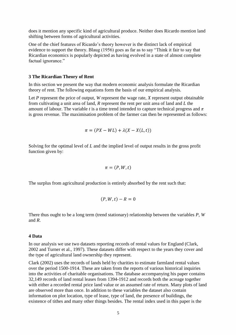
3 The Ricardian Theory of Rent
In this section we present the way that modern economic analysis formulate the Ricardian
theory of rent. The following equations form the basis of our empirical analysis.
Let P represent the price of output, W represent the wage rate, X represent output obtainable
from cultivating a unit area of land, R represent the rent per unit area of land and L the
amount of labour. The variable t is a time trend intended to capture technical progress and π
is gross revenue. The maximisation problem of the farmer can then be represented as follows:
( ) ( ( ))
Solving for the optimal level of L and the implied level of output results in the gross profit
function given by:
( )
The surplus from agricultural production is entirely absorbed by the rent such that:
( )
There thus ought to be a long term (trend stationary) relationship between the variables P, W
and R.
4 Data
In our analysis we use two datasets reporting records of rental values for England (Clark,
2002 and Turner et al., 1997). These datasets differ with respect to the years they cover and
the type of agricultural land ownership they represent.
Clark (2002) uses the records of lands held by charities to estimate farmland rental values
over the period 1500-1914. These are taken from the reports of various historical inquiries
into the activities of charitable organisations. The database accompanying his paper contains
32,149 records of land rental leases from 1394-1912 and records both the acreage together
with either a recorded rental price land value or an assumed rate of return. Many plots of land
are observed more than once. In addition to these variables the dataset also contain
information on plot location, type of lease, type of land, the presence of buildings, the
existence of tithes and many other things besides. The rental index used in this paper is the

6
area-weighted average of all direct rental records and does not include rents derived from
information on land values and an assumed rate of return. The rental index is moreover
incomplete up until the year 1660 and dominated by observations from later time periods.
Rather than interpolate missing observations we decided to analyse the data from the years
1660-1912.
Turner et al (1997) provide historical agricultural rents for 1690-1914. They collect assessed
and received rents from large estates from different sources (estate records, The Royal
Commission on Agriculture and other printed sources). The number of observations per
estate varies significantly. Once more our index is formed by the area-weighted average of
rent received. In addition to these variables the dataset also contain information on plot
location and many other things besides.
Comparing the two datasets, the Turner et al dataset contains observations on 77.1 million
acres while the Clark data set contains observations on 1.1 million acres (2 per cent of the
agricultural land). The Clark index is noticeably higher than the Turner et al one although the
two series move in close harmony with one another. Clark notes that the charity sample is not
entirely representative as charities tend to have smaller than average plot sizes and be located
in more densely-populated areas. Clark (1998) and Turner et al (1998) debate the relative
merits of these two sources of data on rents.
In general, the share of farm tenure is high in England over that period despite the fact that
tenants necessarily have to make investments in the land such as its fertilisation, crops and
fixtures etc.1 Why was not owner-occupation the tenure arrangement of preference? Share-
cropping is when the tenant is too poor to face the uncertainties associated with agricultural
production. Evidence is cited by Offer (1991) that the system of short term tenancies was
increasing and the practice of long term tenancies, or even tenancies in terms of named lives
were falling from around the time of the 16th
century. Nevertheless in bad years landowners
might have allowed tenants’ rents to accumulate. Offer suggests that the prevailing system of
tenure was a device for ensuing that landownership was a stable activity. He reports to the
semblance of a competitive market system for the allocation of tenancies but that turnover of
tenants was low suggesting suggests that the system arose because of the prior appropriation
of land by the elite in the acts of enclosure that commenced around the 16th
century.
The existence of long terms contracts for renting land might mean that the price of
agricultural commodities affects rental prices only in the long run.
Turning to prices, Clark (2004) contains an annual price series for 26 agricultural
commodities in England from 1209-1914. His price index is geometric with weights
corresponding to the output shares of each commodity. These shares are not constant but
nevertheless remain fixed for extended periods. Prices for the same commodity obtained from
different sources are corrected for differences in units of measurement, quality and location.
Sub-indices are provided for arable, meat, dairy, wool, pasture and wood products as well as
an overall farm price index.
In our analysis we use the farm price index as well as prices of individual commodities, most
notably wheat. This is because of uncertainties regarding the weights attached to different
commodities in any overall price index and the fact that, historically, wheat has been the
single most important crop, but partly because of the fact that to be pedantic Ricardo
developed his theory specifically positing a relationship between rental values and the price
of corn.
1 On the eve of the First World War 90 per cent of agricultural land was cultivated by tenant. For a discussion of
the history of the institutional arrangements governing farm tenure from 1750-1950 see Offer (1991).
7
There is a fair correspondence between the agricultural price index and the price index for
wheat. These price indices data reflect the effect of poor weather such as the year without
summer (1815), the Napoleonic wars (1803-1815), the effects of the Corn Laws (1815-1846)
in maintaining prices above the point that they might otherwise have been as well as the
reduction of prices towards the end of the time period caused by the reduction in the price of
ocean going transportation and the influx of imports from Eastern Europe and the New
World.
Farm wage data is taken from Clark (2007) who provides a documented history of
agricultural wages in England from 1209-1869. After 1869 wages are taken from Fox (1903)
who records weekly wages from 125 farms in England and Wales. From 1902-1914 the
agricultural wages are taken from Bowley (1937). These data are then joined together to form
a single wage index.
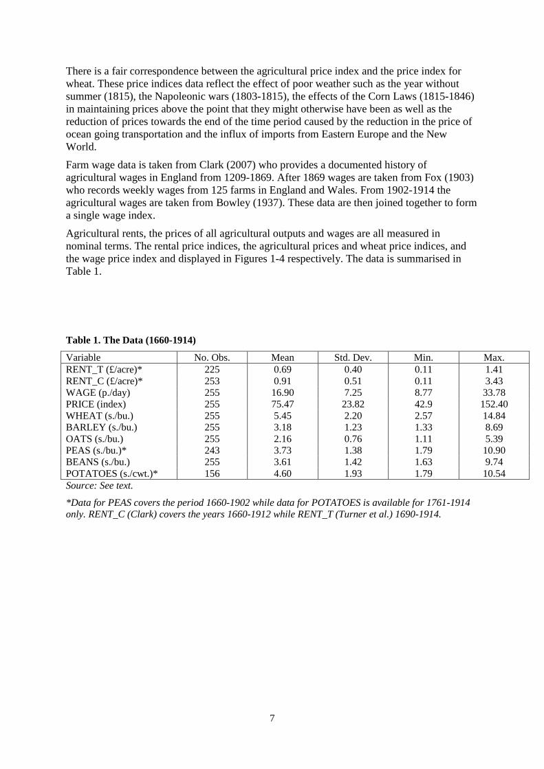
Agricultural rents, the prices of all agricultural outputs and wages are all measured in
nominal terms. The rental price indices, the agricultural prices and wheat price indices, and
the wage price index and displayed in Figures 1-4 respectively. The data is summarised in
Table 1.
Table 1. The Data (1660-1914)
Variable No. Obs. Mean Std. Dev. Min. Max.
RENT_T (£/acre)* 225 0.69 0.40 0.11 1.41
RENT_C (£/acre)* 253 0.91 0.51 0.11 3.43
WAGE (p./day) 255 16.90 7.25 8.77 33.78
PRICE (index) 255 75.47 23.82 42.9 152.40
WHEAT (s./bu.) 255 5.45 2.20 2.57 14.84
BARLEY (s./bu.) 255 3.18 1.23 1.33 8.69
OATS (s./bu.) 255 2.16 0.76 1.11 5.39
PEAS (s./bu.)* 243 3.73 1.38 1.79 10.90
BEANS (s./bu.) 255 3.61 1.42 1.63 9.74
POTATOES (s./cwt.)* 156 4.60 1.93 1.79 10.54
Source: See text.
*Data for PEAS covers the period 1660-1902 while data for POTATOES is available for 1761-1914
only. RENT_C (Clark) covers the years 1660-1912 while RENT_T (Turner et al.) 1690-1914.

8
Figure 1. Agricultural rents in England (1690-1914) Figure 2. Agricultural prices in England (1690-1914)
Figure 3. Farm wages in England (1690-1914) Figure 4. Prices of individual commodities (1690-1914)
01
23
4
Ren
t in
de
x
1700 1750 1800 1850 1900Year
Turner et al. Clark
50
100
150
Pri
ce in
de
x
1700 1750 1800 1850 1900Year
10
15
20
25
30
Farm
wa
ge
(p
en
ce p
er
day)
1700 1750 1800 1850 1900Year
05
10
15
Sh
illin
g
1700 1750 1800 1850 1900year
Wheat Barley Oats Peas Beans Potato
9
5 Empirical Evidence
The main purpose of this paper is to test whether agricultural prices and wage rates Granger
cause agricultural land rents or if rents Granger cause agricultural prices and wage rates (or
both). The Ricardian story is consistent with the finding that agricultural prices and wages
cause rents; it is not consistent with rents causing agricultural prices and wages. Matter are
however different when we consider specific agricultural commodities. Here it is likely that
there is a two-way causal relationship between agricultural rents and the prices of these
commodities. In order to test the direction of Granger causality we adopt methods similar to
those used in the literature albeit in other contexts.
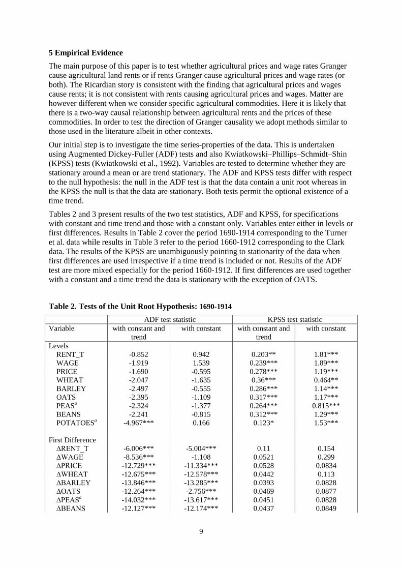
Our initial step is to investigate the time series-properties of the data. This is undertaken
using Augmented Dickey-Fuller (ADF) tests and also Kwiatkowski–Phillips–Schmidt–Shin
(KPSS) tests (Kwiatkowski et al., 1992). Variables are tested to determine whether they are
stationary around a mean or are trend stationary. The ADF and KPSS tests differ with respect
to the null hypothesis: the null in the ADF test is that the data contain a unit root whereas in
the KPSS the null is that the data are stationary. Both tests permit the optional existence of a
time trend.
Tables 2 and 3 present results of the two test statistics, ADF and KPSS, for specifications
with constant and time trend and those with a constant only. Variables enter either in levels or
first differences. Results in Table 2 cover the period 1690-1914 corresponding to the Turner
et al. data while results in Table 3 refer to the period 1660-1912 corresponding to the Clark
data. The results of the KPSS are unambiguously pointing to stationarity of the data when
first differences are used irrespective if a time trend is included or not. Results of the ADF
test are more mixed especially for the period 1660-1912. If first differences are used together
with a constant and a time trend the data is stationary with the exception of OATS.
Table 2. Tests of the Unit Root Hypothesis: 1690-1914
ADF test statistic KPSS test statistic
Variable with constant and
trend
with constant with constant and
trend
with constant
Levels
RENT_T -0.852 0.942 0.203** 1.81***
WAGE -1.919 1.539 0.239*** 1.89***
PRICE -1.690 -0.595 0.278*** 1.19***
WHEAT -2.047 -1.635 0.36*** 0.464**
BARLEY -2.497 -0.555 0.286*** 1.14***
OATS -2.395 -1.109 0.317*** 1.17***
PEASa -2.324 -1.377 0.264*** 0.815***
BEANS -2.241 -0.815 0.312*** 1.29***
POTATOESa -4.967*** 0.166 0.123* 1.53***
First Difference
∆RENT_T -6.006*** -5.004*** 0.11 0.154
∆WAGE -8.536*** -1.108 0.0521 0.299
∆PRICE -12.729*** -11.334*** 0.0528 0.0834
∆WHEAT -12.675*** -12.578*** 0.0442 0.113
∆BARLEY -13.846*** -13.285*** 0.0393 0.0828
∆OATS -12.264*** -2.756*** 0.0469 0.0877
∆PEASa -14.032*** -13.617*** 0.0451 0.0828
∆BEANS -12.127*** -12.174*** 0.0437 0.0849

10
∆POTATOESa -2.227 -2.274** 0.0384 0.103
Note that * means significant at 10 per cent, ** means significant at 5 per cent and *** means
significant at 1 per cent.
*Data for PEAS cover the period 1690-1902 while data for POTATOES is available for 1761-1914
only.
Table 3. Tests of the Unit Root Hypothesis: 1660-1912
ADF test statistic KPSS test statistic
Variable with constant and
trend
with constant with constant and
trend
with constant
Levels
RENT_C -3.175** -1.332 0.2** 1.79***
WAGE -1.515 1.365 0.375*** 2.04***
PRICE -1.879 -1.142 0.219*** 1.32***
WHEAT -2.421 -2.406** 0.3*** 0.542**
BARLEY -2.838* -1.201 0.24*** 1.31***
OATS -2.585 -1.481 0.251*** 1.37***
PEASa -2.741* -2.275** 0.229*** 1.03***
BEANS -2.593 -1.292 0.265*** 1.49***
POTATOESa -5.121*** -0.171 0.132* 1.5***
First Difference
∆RENT_C -20.924*** -0.936 0.0142 0.0142
∆WAGE -10.800*** -9.894*** 0.0391 0.242
∆PRICE -11.044*** -2.123** 0.0706 0.0701
∆WHEAT -12.574*** -3.685** 0.0677 0.073
∆BARLEY -12.946*** -1.282 0.051 0.0503
∆OATS -1.674 -0.333 0.069 0.0691
∆PEASa -14.488*** -14.203*** 0.0541 0.0563
∆BEANS -12.676*** -12.252*** 0.0506 0.0527
∆POTATOESa -10.006*** -10.310*** 0.0263 0.0278
Note that * means significant at 10 per cent, ** means significant at 5 per cent and *** means
significant at 1 per cent. aData for PEAS cover the period 1690-1902 while data for POTATOES cover the period for 1761-
1912.
Next, we investigate if a cointegrating vector exists for our time-series data using the
Johansen cointegration test (with time trend). The trace statistic presented in Table 4 indicates
for r=2 all variables (RENT, WAGE and PRICE) in the two models are stationary.
Table 4. Johansen’s Test for Cointegration
Dataset H0 HA Trace statistic 5 per cent critical value
Turner et al.
(1690-1914)
r=0 R=>1 48.2810 42.44
r=1 R=>2 13.5855* 25.32
r=2 R=>3 3.2691 12.25
Clark
(1660-1912)
r=0 R=>1 137.0456 42.44
r=1 R=>2 24.3009* 25.32
r=2 R=>3 4.5836 12.25

11
In the following, we use the outcome of the test for cointegration to construct a VECM model
explaining the change in the value of each variable as a function of lagged values of all
variable plus an error correction term. Using the VECM it is then possible to test for various
forms of causality. These include short run, long run and overall causality.
For example, in order to test whether prices Granger cause rents it is necessary merely to test
whether the coefficients on the lagged value of ∆P are statistically significant in the equation
for ∆R and whether the variable ECT being the error correction term is statistically significant
for long run causality. For overall causality a test on the statistical significance of both ∆P
and ECT is performed.
∑
∑
∑
Note that the cointegrating regression includes a time trend and the VECM includes a
constant term. Identifying the appropriate number of lags is an important aspect of the model
development process. We use the SBIC criterion to help determine the number of lags. We
evaluate Granger causality for four different models because we have two different series for
agricultural rents and the two different series for agricultural prices. Tables 4a and 4b present
the results. Results of specifications replacing PRICE by WHEAT are presented in the
Appendix (Tables A1-A3). Tables 5a and 5b report the results of the test statistics.
Table 4a. Vector error correction model 1690-1914
∆RENT_Tt ∆PRICEt ∆WAGEt
ECTt-1 -0.0205489
(-3.48)
2.331905
(1.66)
0.0520119
(0.36)
∆RENT_Tt-1 -0.2017747
(-2.98)
13.86479
(0.86)
0.4723812
(0.29)
∆RENT_T t-2 0.0574833
(0.84)
33.68943
(2.06)
1.365067
(0.82)
∆RENT_T t-3 0.0599723
(0.90)
3.479232
(0.22)
-0.9859716
(-0.61)
∆PRICEt-1 0.0001609
(0.53)
0.1063408
(1.46)
0.023666
(3.21)
∆PRICEt-2 -0.0001244
(-0.42)
-0.1997483
(-2.84)
0.0093481
(1.31)
∆PRICEt-3 -0.0002359
(-0.77)
-0.3098356
(-4.27)
0.002045
(0.28)
∆WAGEt-1 0.0091459
(2.94)
1.467431
(1.98)
0.0514365
(0.68)
∆WAGEt-2 0.0021442
(0.68)
-0.6391999
(-0.85)
-0.1414527
(-1.87)
∆WAGEt-3 0.0046643
(1.50)
-0.302238
(-0.41)
-0.0950127
(-1.26)
CONSTANT 0.0024579
(1.31)
-0.0026585
(-0.01)
0.1201631
(2.65)
R-sq 0.1993 0.2341 0.1392
Z-statistics in parenthesis.

12
Table 4b. Vector error correction model 1660-1912 (Clark rent index)
∆RENT_Ct ∆PRICEt ∆WAGEt
ECTt-1 -0.5195037
(-4.73)
-.6078464
(0.26)
-0.5223041
(-2.0)
∆RENT_Ct-1 -0.5199338
(-4.97)
-0.6787084
(-0.30)
0.2791129
(1.12)
∆RENT_Ct-2 -0.472077
(-5.33)
0.2773168
(0.15)
0.104012
(0.49)
∆RENT_C t-3 -0.1710974
(-2.65)
0.8831339
(0.64)
-0.0713745
(-0.47)
∆PRICEt-1 0.0015179
(0.47)
0.0875144
(1.29)
0.0255207
(3.35)
∆PRICEt-2 -0.0001855
(-0.06)
-0.2148213
(-3.26)
0.0116838
(1.58)
∆PRICEt-3 -0.0005962
(-0.19)
-0.3094654
(-4.54)
0.0015305
(0.20)
∆WAGEt-1 0.0331955
(1.15)
1.141521
(1.86)
-0.1920873
(-2.81)
∆WAGEt-2 0.0311049
(1.08)
-0.3434394
(-0.56)
-0.1221928
(-1.79)
∆WAGEt-3 0.0442022
(1.61)
-0.3450663
(-0.59)
-0.0887292
(-1.35)
CONSTANT -0.0732111
(-3.08)
0.0270929
(0.05)
0.0412884
(0.73)
R-sq 0.5501 0.2042 0.1348
Z-statistics in parenthesis.
Table 5a. Chi-sq tests of causality (1690-1914)
RENT_T PRICE WAGE
SR LR Overall SR LR Overall SR LR Overall
RENT_T 4.51 2.75* 5.77 1.27 0.13 1.37
PRICE 1.44 12.11*** 14.78*** 12.97*** 0.13 13.94***
WAGE 10.63** 12.11*** 23.54*** 5.04 2.75* 7.69
Note that * means significant at 10 per cent, ** means significant at 5 per cent and *** means
significant at 1 per cent.
Table 5b. Chi-sq tests of causality (1660-1912)
RENT_C PRICE WAGE
SR LR Overall SR LR Overall SR LR Overall
RENT_C 1.13 0.07 2.43 3.12 3.99** 5.83
PRICE 0.35 22.38*** 27.04*** 14.92*** 3.99** 26.94***
WAGE 3.97 22.38*** 31.76*** 4.85 0.07 5.02
Note that * means significant at 10 per cent, ** means significant at 5 per cent and *** means
significant at 1 per cent.
13
The results of the VECM methodology point unambiguously to a causal relationship running
from prices and wages to rents. But this causal relationship holds only in the long run.
Our explanation for this is the existence of long term rental contracts alluded to earlier. There
is by contrast no evidence to reject the hypothesis of no causal relationship running from
rents to wages or prices. These findings hold irrespective of whether we employ the Clarke or
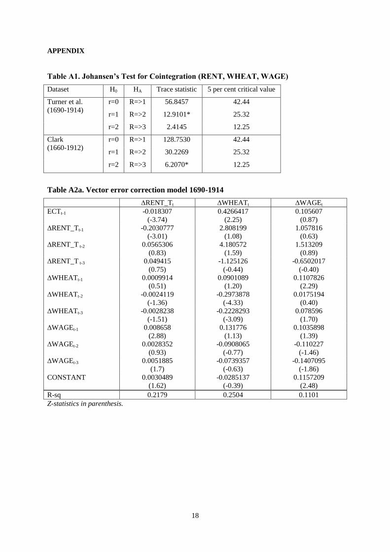
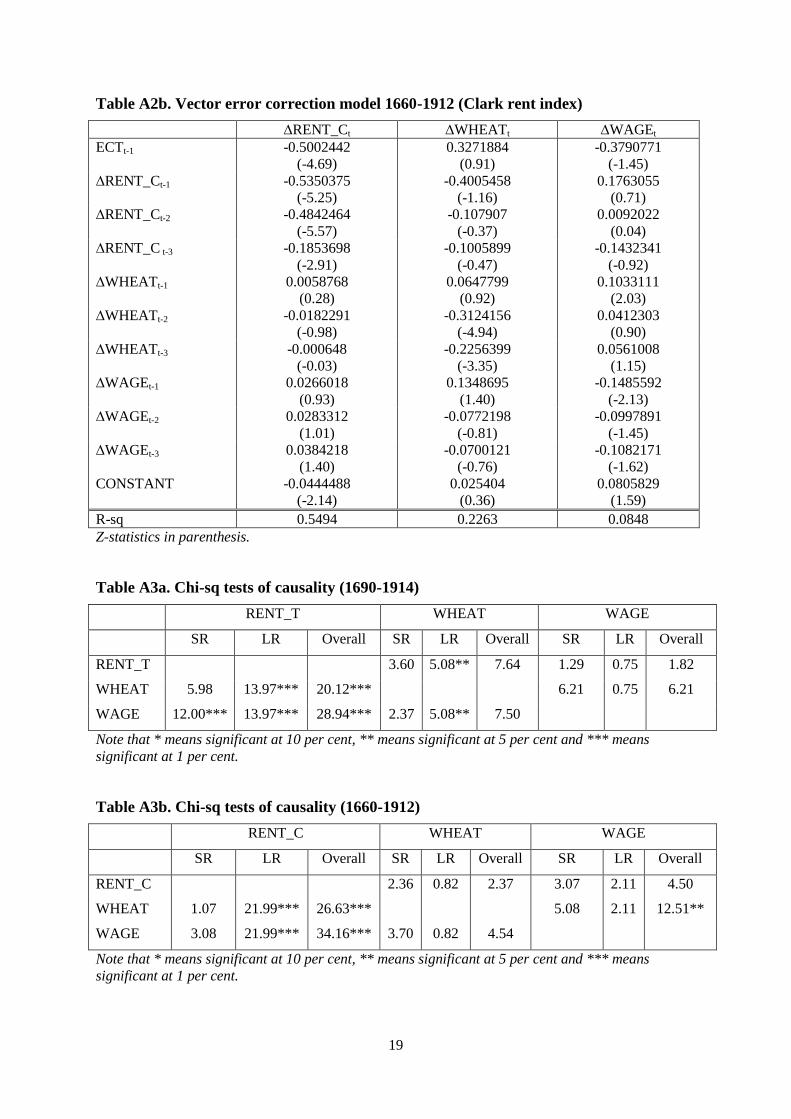
the Turner rent data. When replacing the price index PRICE with the price for WHEAT the
results are unchanged (Tables A1-A3 in the Appendix). Such findings represent very strong
evidence in support of Ricardo’s theory.
There are also some unanticipated findings concerning the existence of a short run
relationship running from prices to wages (for the Clark data also long run). Although
unanticipated it is easy to rationalise this finding in terms of either costs pushing wages or
alternatively it may have an efficiency wage or subsistence interpretation.
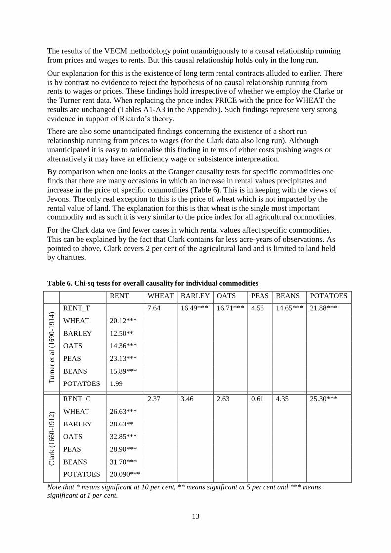
By comparison when one looks at the Granger causality tests for specific commodities one
finds that there are many occasions in which an increase in rental values precipitates and
increase in the price of specific commodities (Table 6). This is in keeping with the views of
Jevons. The only real exception to this is the price of wheat which is not impacted by the
rental value of land. The explanation for this is that wheat is the single most important
commodity and as such it is very similar to the price index for all agricultural commodities.
For the Clark data we find fewer cases in which rental values affect specific commodities.
This can be explained by the fact that Clark contains far less acre-years of observations. As
pointed to above, Clark covers 2 per cent of the agricultural land and is limited to land held
by charities.
Table 6. Chi-sq tests for overall causality for individual commodities
RENT WHEAT BARLEY OATS PEAS BEANS POTATOES
Turn
er e
t al
(1690
-1914)
RENT_T 7.64 16.49*** 16.71*** 4.56 14.65*** 21.88***
WHEAT 20.12***
BARLEY 12.50**
OATS 14.36***
PEAS 23.13***
BEANS 15.89***
POTATOES 1.99
Cla
rk (
16
60
-19
12
)
RENT_C 2.37 3.46 2.63 0.61 4.35 25.30***
WHEAT 26.63***
BARLEY 28.63**
OATS 32.85***
PEAS 28.90***
BEANS 31.70***
POTATOES 20.090***
Note that * means significant at 10 per cent, ** means significant at 5 per cent and *** means
significant at 1 per cent.

14
6 Discussion
Although our focus has been on determining the direction of the causal relation between
prices, wages and rents, our analysis can also be used to measure the rate of technical
progress in agriculture in the period prior even to the industrial revolution. Although ours is
by no means the first attempt to empirically estimate this parameter we believe that it is the
first attempt to do so using an approach based on the link between agricultural profitability
and rental values. Other approaches to estimate the rate of technical progress appear to
employ a production function approach which may be vulnerable to unusual production
conditions at particular locations. By contrast our estimates are much more broadly based and
are estimated over a much longer period of time. Such estimates however derived are
interesting not merely in their own right but because they enable one to comment on the
competing hypotheses of an agricultural revolution taking place contemporaneously with the
industrial revolution (Crafts, 1985) or an early agricultural revolution (Allen, 1999).
In order to obtain estimates of the rate of technical progress in agriculture it is necessary to
adopt a specific functional form. It is convenient to use a Cobb Douglas approximation to the
profit function for this purpose.
The coefficient on the linear time trend T represents the rate of technical progress.
The profit function is meant to be linear homogenous in the price of inputs and outputs. This
restriction can be imposed by insisting that:
( )
In what follows we estimate the rate of technical progress with and without the assumption of
linear homogeneity. We also consider how technical progress in agriculture changed over the
course of the period leading up to the industrial revolution and beyond. Of the many
agricultural inventions perhaps the invention of the threshing machine in 1784 was most
significant since according to Clark (2007) threshing was an activity which absorbed one
quarter of the labour employed in agriculture. We therefore consider separately the periods
pre and post 1784.

15
Table 7. Estimates of the rate of technical progress in agriculture
Turner et al Clark Linear
Homog.
(Turner et al)
Pre-1784
(Turner et al)
Post-1784
(Turner et al)
Ln(R) Ln(R) Ln(R)-Ln(W) Ln(R) Ln(R)
Ln(P) 2.191106
(5.20)
0.9639357
(5.51)
-3.577733
(-5.05)
2.846316
(6.25)
Ln(W) -3.963011
(-4.35)
0.3224256
(1.14)
6.721471
(2.69)
-2.011422
(-2.57)
Ln(P)-Ln(W) 1.698122
(2.91)
YEAR 0.0286024
(5.80)
0.0016014
(1.20)
0.0074864
(3.34)
0.0011895
(0.16)
0.0179264
(3.53)
CONSTANT
Note: P is the farm price index.
The long run parameters are taken from the ECM.
Considering first the estimates obtained from the Turner et al data for the period 1694-1914
we see that the rate of technical progress is 2.8 percent per annum and that this is statistically
significant at even the one percent level of confidence. However, using the Clark data, which
runs from 1664-1914, we see that the rate of technical progress is imprecisely estimated and
not even statistically different from zero at the 10 percent level of confidence.
Reverting once more to the Turner et al data we impose linear homogeneity and obtain an
estimate of 0.7 percent per annum once again significant at the once percent level of
confidence. The imposition of linear homogeneity however results in a very significant loss
of fit meaning that we cannot place much faith in this estimate. Lastly we divide the data into
different time periods. There is no statistically significant level of technical progress over the
period 1694-1784. Over the period 1785-1914 however the rate of technical progress is a
brisk 1.8 percent per annum. It does therefore appear that there is little evidence in favour of
an early agricultural revolution as envisaged by Allen (1999).
7 Conclusions
One of Ricardo’s most important contributions to economics is establishing the link between
wages, prices and rents. But despite its importance to both historians and analysts making
pronouncements based on the Ricardian hypothesis there have been no attempts to
empirically validate the underlying assumption that changes in aggregate prices simply feed
through into changed prices for rents. This paper has employed recently obtained historical
data to test the key proposition put forward by Ricardo. The results strongly support
Ricardo’s great insight whilst at the same time upholding the contrary view put forward by
amongst others that other great 19th
century economist Jevons. Basically the overall price of
agricultural commodities causes land rents but, in the case of individual agricultural
commodities, this causality runs in both directions. This provides empirical confirmation of
one of the most important insights of agricultural economics and something contained in
every agricultural economics textbook: the idea of rent as a ‘residual’.
Such findings provide further insight into the effects of the Corn Laws i.e. the belief that the
effect of maintaining protection from low-cost imports would have benefitted landowners.
There is even confirmation of another effect identified by amongst others Ricardo, namely
the impact of higher agricultural prices on the agricultural wage. It is clear that the increase in
agricultural wages following an increase in agricultural prices is at least consistent with

16
Ricardo’s subsistence view of wages and the idea of higher prices cutting the labour force
until the nominal wage rate has risen enough to restore the real value of wages.
The same data also provides an estimate of the rate of technical progress measured over a
very lengthy period of time. The estimates point to a period of rapid technical progress over
the period as a whole but progress that is most discernible only after the period of one of the
most important agricultural innovations. These results do not give any support to the view
that the agricultural revolution was in any sense out of synch with the wider industrial
revolution.
Although the data that have been used to undertake these analyses are remarkable they are
not unique. Similar data exist for other European countries and it would of course be
interesting to repeat the analyses contained in this paper using data from elsewhere.
Bibliography
Allen, R.C. (1999), Tracking the agricultural revolution in England, The Economic History
Review, 52(2), 209-235.
Alyousha. A, and Tsoukis, C. (1998), Ricardian ordering and the relation between house and
land prices: evidence from England, Applied Economic Letters (5), 325-328.
Blaug, M. (1956), The Empirical Content of Ricardian Economics”, Journal of Political
Economy, Vol. 64, No. 1 (Feb., 1956), 41-58.
Buchanan, D. H. (1929), The Historical Approach to Rent and Price Theory, Economica, No.
26 (Jun., 1929), 123-155.
Bowley, A.L. (1937), Wages and Income in the United Kingdom since 1860, Cambridge
University Press
Clark. G, (2007), The long march of history: Farm wages, population, and economic growth,
England 1209-1869 -super-1, Economic History Review, Economic History Society, vol.
60(1), 97-135, 02.
Clark, G. (1998), Renting the revolution, Journal of Economic History 58(1), 206-210.
Clark. G, (2004), The price history of English agriculture, 1209-1914, Research in Economic
History, Volume 22, Emerald Group Publishing Limited, 41 – 123.
Clark. G, (2002), Land rental values and the agrarian economy: England and Wales, 1500-
1914, European Review of Economic History, 6, 281–308.
Crafts, N.F.R. (1985), British economic growth during the industrial revolution, Clarendon
Press
Fox, (1903), Agricultural Wages in England and Wales during the Last Fifty Years, Journal
of the Royal Statistical Society, Vol. 66, No. 2 , 273-359.
Kwiatkowski, D., Phillips, P.C.B., Schmidt, P. and Shin, Y. (1992), Testing the Null
Hypothesis of Stationarity against the Alternative of a Unit Root. Journal of Econometrics 54,
159–178.
Malthus, R. (1798), An Essay on the Principle of Population, 1st ed. J Johnson, London.
Oikarinen, E. (2009), Dynamic linkages between housing and lot prices: Empirical evidence
from Helsinki, Discussion Papers 53, Aboa Centre for Economics.

17
Ooi, J. T. L. and Lee, S. (2006), Price discovery between residential land and housing
markets, Journal of Housing Research, 15(2), 95–112.
Ricardo, D. (1821), Principles of Political Economy and Taxation, 3rd ed. John Murray,
London.
Rossini. P, and Kupke. V (2012), Granger Causality Test for the relationship between house
and land prices, Eighteen Annual Pacific-Rim real estate society conference.
Samuelson, P. (1959), A Modern Treatment of the Ricardian Economy: I. The Pricing of
Goods and of Labor and Land Services The Quarterly Journal of Economics, Vol. 73, No. 1
(Feb., 1959), 1-35.
Sraffa, P. (1960), Production of Commodities by Means of Commodities, Cambridge
University Press
Turner, M., Beckett, J. and Afton, B. (1998), Renting the revolution: A reply to Clark,
Journal of Economic History 58(1), 211-214.
Turner, M., Beckett, J. and Afton, B. (1997), Agricultural rent in England: 1690-1914,
Cambridge University Press.
Offer, A. (1991), The First World War: An Agrarian Interpretation, Oxford University Press.
18
APPENDIX
Table A1. Johansen’s Test for Cointegration (RENT, WHEAT, WAGE)
Dataset H0 HA Trace statistic 5 per cent critical value
Turner et al.
(1690-1914)
r=0 R=>1 56.8457 42.44
r=1 R=>2 12.9101* 25.32
r=2 R=>3 2.4145 12.25
Clark
(1660-1912)
r=0 R=>1 128.7530 42.44
r=1 R=>2 30.2269 25.32
r=2 R=>3 6.2070* 12.25
Table A2a. Vector error correction model 1690-1914
∆RENT_Tt ∆WHEATt ∆WAGEt
ECTt-1 -0.018307
(-3.74)
0.4266417
(2.25)
0.105607
(0.87)
∆RENT_Tt-1 -0.2030777
(-3.01)
2.808199
(1.08)
1.057816
(0.63)
∆RENT_T t-2 0.0565306
(0.83)
4.180572
(1.59)
1.513209
(0.89)
∆RENT_T t-3 0.049415
(0.75)
-1.125126
(-0.44)
-0.6502017
(-0.40)
∆WHEATt-1 0.0009914
(0.51)
0.0901089
(1.20)
0.1107826
(2.29)
∆WHEATt-2 -0.0024119
(-1.36)
-0.2973878
(-4.33)
0.0175194
(0.40)
∆WHEATt-3 -0.0028238
(-1.51)
-0.2228293
(-3.09)
0.078596
(1.70)
∆WAGEt-1 0.008658
(2.88)
0.131776
(1.13)
0.1035898
(1.39)
∆WAGEt-2 0.0028352
(0.93)
-0.0908065
(-0.77)
-0.110227
(-1.46)
∆WAGEt-3 0.0051885
(1.7)
-0.0739357
(-0.63)
-0.1407095
(-1.86)
CONSTANT 0.0030489
(1.62)
-0.0285137
(-0.39)
0.1157209
(2.48)
R-sq 0.2179 0.2504 0.1101
Z-statistics in parenthesis.
19
Table A2b. Vector error correction model 1660-1912 (Clark rent index)
∆RENT_Ct ∆WHEATt ∆WAGEt
ECTt-1 -0.5002442
(-4.69)
0.3271884
(0.91)
-0.3790771
(-1.45)
∆RENT_Ct-1 -0.5350375
(-5.25)
-0.4005458
(-1.16)
0.1763055
(0.71)
∆RENT_Ct-2 -0.4842464
(-5.57)
-0.107907
(-0.37)
0.0092022
(0.04)
∆RENT_C t-3 -0.1853698
(-2.91)
-0.1005899
(-0.47)
-0.1432341
(-0.92)
∆WHEATt-1 0.0058768
(0.28)
0.0647799
(0.92)
0.1033111
(2.03)
∆WHEATt-2 -0.0182291
(-0.98)
-0.3124156
(-4.94)
0.0412303
(0.90)
∆WHEATt-3 -0.000648
(-0.03)
-0.2256399
(-3.35)
0.0561008
(1.15)
∆WAGEt-1 0.0266018
(0.93)
0.1348695
(1.40)
-0.1485592
(-2.13)
∆WAGEt-2 0.0283312
(1.01)
-0.0772198
(-0.81)
-0.0997891
(-1.45)
∆WAGEt-3 0.0384218
(1.40)
-0.0700121
(-0.76)
-0.1082171
(-1.62)
CONSTANT -0.0444488
(-2.14)
0.025404
(0.36)
0.0805829
(1.59)
R-sq 0.5494 0.2263 0.0848
Z-statistics in parenthesis.
Table A3a. Chi-sq tests of causality (1690-1914)
RENT_T WHEAT WAGE
SR LR Overall SR LR Overall SR LR Overall
RENT_T 3.60 5.08** 7.64 1.29 0.75 1.82
WHEAT 5.98 13.97*** 20.12*** 6.21 0.75 6.21
WAGE 12.00*** 13.97*** 28.94*** 2.37 5.08** 7.50
Note that * means significant at 10 per cent, ** means significant at 5 per cent and *** means
significant at 1 per cent.
Table A3b. Chi-sq tests of causality (1660-1912)
RENT_C WHEAT WAGE
SR LR Overall SR LR Overall SR LR Overall
RENT_C 2.36 0.82 2.37 3.07 2.11 4.50
WHEAT 1.07 21.99*** 26.63*** 5.08 2.11 12.51**
WAGE 3.08 21.99*** 34.16*** 3.70 0.82 4.54
Note that * means significant at 10 per cent, ** means significant at 5 per cent and *** means
significant at 1 per cent.
Top Related