


Languages
Pages
Legal


University of New South Wales
School of Economics
Honours Thesis
Credit Ratios and the Real Economy
A Time Series Analysis Using US Data
Author:
Isabel Hartstein
Student ID: 3462932
Supervisors:
Prof. James Morley
A/Prof. Glenn Otto
Bachelor of Economics (Economics and Financial Economics) (Honours)
and
Bachelor of Commerce (Finance)

Declaration
I declare that this thesis is my own work and that, to the best of my knowledge, it
contains no material which has been written by another person or persons, except
where acknowledgement has been made. This thesis has not been submitted for the
award of any degree or diploma at the University of New South Wales Sydney, or
at any other institute of higher education.
. . . . . . . . . . . . . . . . . . . . . . . . . . . . . . . . . .
Isabel Hartstein
31st October, 2017
i

Acknowledgements
To my supervisors James Morley and Glenn Otto, thank you so much for all the
time and effort you took to offer guidance and answer my questions this year. I am
grateful for your patience and insights. I finish this year with a greater set of skills,
knowledge and understanding of economics and econometrics than when I started.
I also take with me a greater appreciation of the challenges, rigour and reward of
research. For all your wisdom, critiques and lessons, thank you!
To Barath, Beatrix, Bill, Binal, Helena, Sarah and Simon, I could not have asked
for better company to share this year with. I am grateful for how we pulled together
when the work was difficult, and even more grateful for the conversations, joking,
card games and all-round entertainment when the work grew more difficult. This
year would have been a lot less rewarding without all of you!
To Tess Stafford and Geni Dechter, thank you for your help and feedback throughout
the workshops and practice presentations. I appreciate all the effort you went to for
the Honours cohort.
I would like to thank the Reserve Bank of Australia as well as the UNSW Business
School for the generous financial support I received this year.
To Mum and Dad, thank you for supporting my education and imparting a love of
learning. To Eleanor and James, thank you for your encouragement throughout the
year, as well as the distractions.
ii
Contents
List of Tables v
List of Figures vi
Abstract 1
1 Introduction 2
2 Literature Review 5
2.1 Financial Development and Cross-Sectional Studies . . . . . . . . . . 5
2.2 The Time Series Approach . . . . . . . . . . . . . . . . . . . . . . . . 7
2.3 A Weakening Long Run Relationship? . . . . . . . . . . . . . . . . . 8
3 Data 11
4 Cointegration Analysis 15
4.1 Unit Root Tests . . . . . . . . . . . . . . . . . . . . . . . . . . . . . . 15
4.2 Engle-Granger Test . . . . . . . . . . . . . . . . . . . . . . . . . . . . 17
4.3 Johansen Test . . . . . . . . . . . . . . . . . . . . . . . . . . . . . . . 19
4.4 VECM Analysis . . . . . . . . . . . . . . . . . . . . . . . . . . . . . . 20
4.4.1 Impulse Responses . . . . . . . . . . . . . . . . . . . . . . . . 23
5 Unobserved Components Model 26
5.1 Unobserved Components Model for Cointegration . . . . . . . . . . . 28
5.1.1 Estimation . . . . . . . . . . . . . . . . . . . . . . . . . . . . . 30
5.1.2 Identification . . . . . . . . . . . . . . . . . . . . . . . . . . . 32
5.1.3 Results . . . . . . . . . . . . . . . . . . . . . . . . . . . . . . . 33
5.1.4 Unobserved Components Model with 2 Stochastic Trends . . . 34
5.2 Unobserved Components Model with 3 Stochastic Trends . . . . . . . 36
5.2.1 Results . . . . . . . . . . . . . . . . . . . . . . . . . . . . . . . 39
5.3 Discussion of Findings . . . . . . . . . . . . . . . . . . . . . . . . . . 43
5.3.1 Robustness to the Global Financial Crisis . . . . . . . . . . . 46
iii
6 VAR of First Differences 49
6.1 Granger Causality Tests . . . . . . . . . . . . . . . . . . . . . . . . . 50
6.2 Impulse Responses: Short and Long Run Restrictions . . . . . . . . . 50
7 Conclusion 55
A Cointegration Analysis and VECM 57
A.1 Unit Root Tests . . . . . . . . . . . . . . . . . . . . . . . . . . . . . . 57
A.2 Additional Engle-Granger Test . . . . . . . . . . . . . . . . . . . . . . 58
A.3 VECM Short Term Effects . . . . . . . . . . . . . . . . . . . . . . . . 58
B VAR 59
B.1 VAR Estimates . . . . . . . . . . . . . . . . . . . . . . . . . . . . . . 59
B.2 Structural Identification . . . . . . . . . . . . . . . . . . . . . . . . . 60
iv

List of Tables
4.1 ADF Tests for Unit Roots . . . . . . . . . . . . . . . . . . . . . . . . 16
4.2 Engle-Granger Test with Disaggregated Credit Ratios . . . . . . . . . 18
4.3 Engle-Granger Test with Aggregate Credit Ratio . . . . . . . . . . . . 19
4.4 Johansen Tests . . . . . . . . . . . . . . . . . . . . . . . . . . . . . . 21
4.5 VECM Estimates . . . . . . . . . . . . . . . . . . . . . . . . . . . . . 22
5.1 Unobserved Components Model for Cointegration . . . . . . . . . . . 34
5.2 Unobserved Components Model with 2 Stochastic Trends . . . . . . . 37
5.3 Unobserved Components Model with 3 Stochastic Trends . . . . . . . 41
5.4 Comparing the Persistence of Transitory Components . . . . . . . . . 44
5.5 Unobserved Components Model For 1952:Q1-2008:Q1 . . . . . . . . . 46
6.1 Granger Causality Tests . . . . . . . . . . . . . . . . . . . . . . . . . 51
A.1 ADF-GLS Tests for Unit Roots . . . . . . . . . . . . . . . . . . . . . 57
A.2 KPSS Tests for Unit Roots . . . . . . . . . . . . . . . . . . . . . . . . 57
A.3 ADF Tests for Unit Roots of First Differences . . . . . . . . . . . . . 57
A.4 Engle-Granger Test for Household Credit and Firm Credit . . . . . . 58
A.5 Lagged Parameter Estimates for VECM . . . . . . . . . . . . . . . . 58
B.1 Parameter Estimates for VAR in First Differences . . . . . . . . . . . 59
v

List of Figures
3.1 US Real GDP and the Credit Ratios . . . . . . . . . . . . . . . . . . 13
3.2 US Real GDP Growth and Differenced Credit Ratios . . . . . . . . . 14
4.1 Cointegrating Error . . . . . . . . . . . . . . . . . . . . . . . . . . . . 17
4.2 VECM Impulse Response Functions . . . . . . . . . . . . . . . . . . . 25
5.1 Impulse Response Functions for Transitory Components with Coin-
tegration . . . . . . . . . . . . . . . . . . . . . . . . . . . . . . . . . . 35
5.2 Impulse Response Functions for Transitory Components with 3
Stochastic Trends . . . . . . . . . . . . . . . . . . . . . . . . . . . . . 42
5.3 Impulse Response Functions for Transitory Components of 1952:Q1-
2008:Q1 Sample . . . . . . . . . . . . . . . . . . . . . . . . . . . . . . 47
6.1 VAR Impulse Response Functions Using Short Run Restrictions . . . 52
6.2 VAR Impulse Response Functions Using Long Run Restrictions . . . 54
vi

Abstract
This thesis examines the long run relationship between real GDP and the ratios
of household credit and firm credit to GDP in the United States. I develop an
unobserved components model to evaluate whether permanent movements in the
credit ratios cause permanent movements in real GDP. Comparing these results with
a vector error correction model and a vector auto-regression, I find the credit ratios
and real GDP are not cointegrated, and the credit ratios do not have permanent
effects on real GDP. Real GDP may have positive transitory effects on the credit
ratios, but there is no robust evidence to indicate these effects are permanent. The
absence of any substantive correlation between the permanent movements in the
credit ratios and real GDP suggests there is no long run relationship. This supports
recent findings in the financial development literature that the long run relationship
between finance and economic growth is weaker in advanced economies.
1

Section 1
Introduction
Across the world total credit to the private sector has expanded more quickly than
Gross Domestic Product (GDP). The ratio of private credit to GDP is the standard
measure of financial development. Since the 1990s, a large empirical literature has
shown financial development to be not only a by-product of economic growth, but
also a key factor driving long run economic growth (see Levine, 2005). To the extent
it reflects financial development, a growing ratio of private credit to GDP is generally
considered beneficial.
This long run relationship has come under greater scrutiny, particularly in the
aftermath of the Global Financial Crisis. The relationship between the credit ratio
and economic growth is found to be weaker in high-income countries compared
to middle-income countries (Rioja and Valev, 2004). The relationship may also be
weaker where a greater share of credit is allocated to households instead of businesses
(Beck, Buyukkarabacak, Rioja, and Valev, 2012). These findings highlight the
inherent flaw of using credit ratios as an indicator of financial development, when
in reality credit ratios are a measure of financial depth.
This thesis examines whether the ratios of household credit and firm credit to
GDP have permanent effects on real GDP in the United States. Using a variety
of time series models, I find no long run relationship. Credit ratios do not have
permanent effects on real GDP and real GDP does not have permanent effects on
credit ratios either. There is evidence to suggest real GDP has transitory effects
on the credit ratios, since higher levels of aggregate income encourages temporarily
higher borrowing. The household credit ratio may also have a positive transitory
effect on real GDP, however, there is no robust evidence that on average permanent
movements in the credit ratios cause permanent movements in real GDP.
This thesis contributes to the literature in two ways. First, I use disaggregated credit
data rather than the typical aggregate measure of total credit to the private sector.
I find that disaggregating the total credit ratio into household and firm borrower
groups gives clearer evidence of stochastic trends in the credit ratios. This could
be due to movements in household credit and firm credit coincidentally offsetting
2

each other historically, resulting in a weaker signal of permanent movements in the
aggregate credit ratio.
Second, I use a variety of time series models to examine the long run trends in the
data. I begin by estimating a vector error correction model (VECM) as there is
mixed evidence of cointegration. I find that real GDP is weakly exogenous. Using
the unobserved components model, I determine that the credit ratios and real GDP
are not cointegrated. This model provides a means of decomposing a time series into
its permanent (stochastic trend) and transitory (stationary) components. It provides
a more parsimonious specification due to the substantial degree of persistence in the
credit ratios and has two important features. First, it allows for correlation between
the movements of the permanent and transitory components both within a series
and across series. These correlations reflect the temporary adjustment of a variable
to a new long run level following a permanent shock. Second, it allows for each
variable to have a different speed of adjustment to a shock. I consistently find that
real GDP adjusts more quickly than the credit ratios. Finally, I estimate a vector
auto-regression (VAR) of the first differences as a robustness check of the findings.
The multivariate unobserved components model I develop is novel. It extends
previous correlated unobserved components models (see Morley, 2007; Sinclair, 2009)
to a higher dimension and allows each variable to have a unique stochastic trend
that forms part of the permanent component of another variable. It is the ordering
of the variables that determines how this occurs. I find it is best to allow real
GDP to drive permanent movements in the credit ratios. There is a slight positive
correlation between permanent movements in real GDP and transitory movements
in the credit ratios, however, there does not appear to be a statistically significant
correlation between the permanent movements. This suggests that there is no long
run relationship between the credit ratios and real GDP in the United States.
The typical approach in the literature is to exploit cross-country variation and
estimate a dynamic panel (see Beck, 2009). Instead, I exploit variations in the
data across time in a single country. Panel studies mask the large degree of country
heterogeneity. The United States provides an interesting case study as it is an
advanced economy at the technology frontier and may be representative of similar
advanced economies.
These results support the growing body of empirical research in the financial
development literature that the long run finance-growth relationship is weaker in
advanced economies. The implication is that when using credit ratios to capture
3

financial deepening (or possibly financial development), greater financial depth is not
driving the long run level of output in the United States. This approach could be
applied to more countries to see if this finding extends to other advanced economies.
4
Section 2
Literature Review
The contribution of the financial system to long run economic growth is an ongoing
point of contention. In his survey of the literature, Ang (2008) traces the idea that
financial development causes economic growth to Joseph Schumpeter in 1911. In
the 1970s, this idea inspired the inclusion of financial intermediaries in economic
growth models by McKinnon (1973) and Shaw (1973), which provided a theoretical
basis for greater financial liberalisation. Neoclassical growth models emphasised the
role of technology, labour and capital accumulation, and gave little importance to
the financial sector. The leading neoclassical economist Robert Lucas, described
the role of financial system as “badly over-stressed” (King and Levine, 1993). The
development of endogenous growth models saw new models (such as Greenwood
and Jovanovic, 1990; Pagano, 1993) present financial intermediaries as a key factor
driving endogenously determined technology.
2.1 Financial Development and Cross-Sectional Studies
To explain the role of the financial system as a driver of long run economic
output, it is important to first define financial development. Levine (2005)
defines financial development as occurring when “financial instruments, markets,
and intermediaries ameliorate . . . the effects of information, enforcement, and
transactions costs and therefore do a correspondingly better job at providing the
five financial functions”. These five functions are i) producing information about
investments, ii) monitoring investments, iii) mobilising savings, iv) diversifying risk
and v) facilitating payments. As financial systems develop these functions, the costs
of transactions and overcoming information asymmetries should decline, resulting
in a more efficient allocation of savings to the most productive investments. In this
way, financial development should boost economic growth by driving productivity,
as well as facilitating the accumulation of physical capital.
Beginning with the work of King and Levine (1993), the empirical research into
the finance-growth nexus has primarily focussed on cross-countries studies. Using
ordinary least squares (OLS) regressions, the authors find a positive relationship
between financial development and GDP per capita growth for 77 countries from
5

1960-89. To capture financial development, the authors measure the size of the
formal financial sector relative to GDP. Since Levine, Loayza, and Beck (2000), the
ratio of private credit to GDP has emerged as the standard measure of financial
development. Private credit is the value of credit issued by banks and other
regulated financial intermediaries to the private sector. This excludes credit issued
to governments and credit issued by central banks (Levine, 2005).
While higher levels of the credit ratio is correlated with lower interest margins
and transaction costs, it is fundamentally a measure of financial depth, not the
quality of financial services and institutions. In part it is popular since it can
be calculated over long periods of time for many countries at different stages of
economic development. However, financial development is not a linear function of
financial depth. Short term variations in credit may reflect credit bubbles rather
than systematic improvements in financial systems. In this thesis, I use a newer
measure of the credit ratio disaggregated into household credit and firm credit from
the Bank of International Settlements (BIS). Due to the problematic interpretation
of the credit ratio as financial development, I simply interpret the credit ratio as a
measure of financial depth. Consequently, this analysis of the credit ratio and real
GDP has implications for the economic role of financial depth.
Aside from the measurement of financial development, a key issue for the empirical
literature has been identifying exogenous changes in credit. The central criticism
of the early OLS regressions, was the issue of reverse causality resulting in biased
and inconsistent estimators. The credit ratio is typically included as a regressor
rather than the dependent variable. This is problematic given economic growth
is likely to cause growth in demand for financial services. To address the issue of
reverse causation, researchers have adopted panel techniques, specifically two-step
generalised method of moments (GMM) (see Beck et al., 2012; Levine et al., 2000;
Rioja and Valev, 2004). Another popular approach has been difference-in-differences
estimation. For example, Jayaratne and Strahan (1996) exploit the variation in bank
branch regulations across states in the U.S. from 1970-95 and examine its effects on
state-level growth. The seminal paper by Rajan and Zingales (1998) uses variation
in industry growth rates to test whether industries with a greater dependence on
external finance grow faster in countries with a more developed financial system.
While such techniques are an improvement on standard OLS regressions, these
approaches have limitations. As Beck (2009) notes, GMM and difference-in-
differences estimators are inconsistent if instruments for financial development are
not valid. Omitted variable bias is also a possible problem. This can be mitigated
6

using panel techniques to remove time-invariant factors and by including control
variables, however, limited degrees of freedom can make this difficult. Difference-
in-differences estimation requires several assumptions to overcome omitted variable
bias. Jayaratne and Strahan (1996) assume state-inherent characteristics are time
invariant, while Rajan and Zingales (1998) assume industry-inherent characteristics
do not vary across countries.
2.2 The Time Series Approach
Time series analysis uses variation across time periods rather than countries to
examine causality. It is less common in the literature as it relies on higher frequency
data across a sufficiently large time period. This is often lacking for developing
countries. The time series approach differs from panel studies in several fundamental
ways. First, time series models such as a vector auto-regression (VAR) treat all
variables as endogenous. Second, rather than controlling for multiple variables, or
finding appropriate instruments, omitted variable bias is addressed by allowing for
a sufficient number of lags, so the error term is serially uncorrelated.
In these time series analyses, causality is tested in the sense of whether financial
development Granger-causes economic growth. If so, the lagged values of the credit
ratio should contain information which can forecast the current value of economic
growth, while controlling for the lagged values of economic growth. Luintel and
Khan (1999) examine the long run finance-growth relationship of 10 developing
countries using a vector error correction model (VECM) to test for cointegration
and the weak exogeneity of finance. They find evidence of bi-directional causality
and a stable, positive long-run relationship. To increase sample size, Christopoulos
and Tsionas (2004) use panel data for 10 developing countries. The authors find a
single cointegration vector and conclude there is evidence of causality from financial
development to economic growth, which is not bi-directional. In another application
of cointegration and Granger-causality tests, Fink, Haiss, and Hristoforova (2003)
consider the effect of bond market development on real GDP in advanced economies
from 1950 to 2000. For most countries, including the United States, the authors
find bond market development leads economic growth. This finding also highlights
the importance of bond markets as a source of credit, in addition to bank lending.
An advantage of a time series approach is that it allows for variation in the finance-
growth relationship across countries. Panel regressions assume the relationship
between finance and growth is identical across countries, that is, the parameter
governing the relationship βi = β for all countries i (Beck, 2009). Time series
7
studies such as Luintel, Khan, Arestis, and Theodoridis (2008) reveal a considerable
amount of country heterogeneity which is often masked by pooling information
across countries. Focussing on a single country can reveal patterns of causality
not evident from panel studies. In this thesis, I focus solely on the United States.
The United States is an inherently interesting case as it is an advanced economy. It
is these economies where there is growing evidence of a weakening long run finance-
growth relationship.
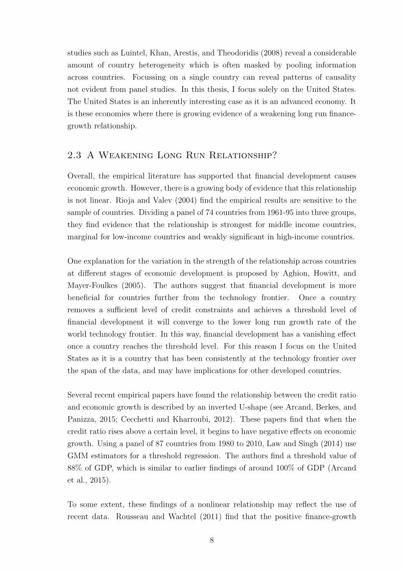
2.3 A Weakening Long Run Relationship?
Overall, the empirical literature has supported that financial development causes
economic growth. However, there is a growing body of evidence that this relationship
is not linear. Rioja and Valev (2004) find the empirical results are sensitive to the
sample of countries. Dividing a panel of 74 countries from 1961-95 into three groups,
they find evidence that the relationship is strongest for middle income countries,
marginal for low-income countries and weakly significant in high-income countries.
One explanation for the variation in the strength of the relationship across countries
at different stages of economic development is proposed by Aghion, Howitt, and
Mayer-Foulkes (2005). The authors suggest that financial development is more
beneficial for countries further from the technology frontier. Once a country
removes a sufficient level of credit constraints and achieves a threshold level of
financial development it will converge to the lower long run growth rate of the
world technology frontier. In this way, financial development has a vanishing effect
once a country reaches the threshold level. For this reason I focus on the United
States as it is a country that has been consistently at the technology frontier over
the span of the data, and may have implications for other developed countries.
Several recent empirical papers have found the relationship between the credit ratio
and economic growth is described by an inverted U-shape (see Arcand, Berkes, and
Panizza, 2015; Cecchetti and Kharroubi, 2012). These papers find that when the
credit ratio rises above a certain level, it begins to have negative effects on economic
growth. Using a panel of 87 countries from 1980 to 2010, Law and Singh (2014) use
GMM estimators for a threshold regression. The authors find a threshold value of
88% of GDP, which is similar to earlier findings of around 100% of GDP (Arcand
et al., 2015).
To some extent, these findings of a nonlinear relationship may reflect the use of
recent data. Rousseau and Wachtel (2011) find that the positive finance-growth
8

relationship is not as robust when including data since the 1990s compared to
the original panel studies that used data from 1960-90. To explain this result,
the authors also find strong evidence that financial crises weaken the relationship
between financial deepening and economic growth. These findings highlight the
important role institutions and regulatory agencies play in preventing financial
crises. I also consider the impact of the Global Financial Crisis by comparing the
results of the unobserved components model using the full sample to a shorter sample
period ending in 2008.
There exists a considerable literature on the severity of financial crises following
credit expansions. Using data from 1870-2008 for advanced economies, Jorda,
Schularick, and Taylor (2013) find recessions resulting from financial crises are
more devastating than typical recessions, and deeper recessions follow more credit-
intensive expansions. The large literature on business cycle volatility and credit,
appears to undermine the policy implications of the financial development literature.
To account for these differing long run and short run effects, Loayza and Ranciere
(2006) analyse the finance-growth relationship using an auto-regressive distributed
lag (ARDL) model. Using data for multiple countries at different stages of
development, the long run effect is first estimated using a pooled mean group
estimator, and is found to be positive. The coefficients of the lagged credit ratio
capture short run effects, and are negative in financially fragile countries. In the
long run, higher credit ratios are broadly associated with higher levels of economic
development, but in the short run may predict financial instability.
These findings highlight a contradiction between studies that focus on the long
run finance-growth relationship, and those that consider the relationship over the
business cycle. I focus on the long run relationship while also allowing for short term
dynamics. This is an advantage of using time series models. The VECM captures
short run dynamics in addition to the long run cointegrating relationship. I also
estimate an unobserved components model which allows for correlation between the
permanent and transitory movements within a variable as well as across variables.
The emphasis though is on finding common permanent movements in real GDP and
the credit ratios.
Another related reason for a weakening long run relationship between the credit
ratio and economic growth is the allocation of credit. The aggregate measure of
credit to the private sector as a proportion of GDP encompasses loans to households
as well as firms. In theory, allocating credit to firms rather than households
should drive economic growth as credit can be used more productively. Hung
9

(2009) presents a model that replicates the nonlinear relationship between financial
development and economic growth by the composition of aggregate credit. In this
model of asymmetric information, financial development alleviates information and
monitoring costs, and also facilitates productive investment loans as well as non-
productive consumption loans. The nature of the relationship between financial
development and economic growth is determined by the relative magnitude of these
two types of loans.
A key empirical feature of credit ratios in high-income countries is the changing
composition of credit towards households. Greenwood and Scharfstein (2013)
document the growth of the financial services sector in the United States from 1980
to 2007. They find that the growth of finance is primarily the result of the growth
in asset management and the provision of household credit. They also find that
household credit grew from 48% of GDP in 1980 to 99% of GDP in 2007, mostly
due to residential mortgages. Philippon and Reshef (2013) also document a rise is
the size of the financial services sector across advanced economies.
Due to the limited availability of disaggregated credit data across countries at
various stages of economic development, the vast majority of empirical research
uses the aggregate measure of private credit. Some recent empirical research has
used disaggregated credit data. Beck et al. (2012) construct a dataset of 45 countries
and decompose bank lending into household and firm lending. Using various cross-
country regressions the authors conclude that firm credit is positively related to
economic growth but household credit is not. Sassi and Gasmi (2014) use a
panel of European Union countries from 1995-2012 and similarly find enterprise
credit has positive effects while household credit has a negative effect on economic
growth. To capture potentially different effects, I also use credit data that has been
disaggregated into household and firm borrower groups.
10

Section 3
Data
I use a measure of private credit sourced from the BIS “Long series on credit to
the private non-financial sector” database.1 The key characteristics of credit are
the lender, financial instrument and borrower. Lenders include domestic banks,
the non-bank financial sector and foreign banks that provide cross-border lending.
Financial instruments include loans and debt securities such as bonds and short-
term paper. Outstanding loans are measured at nominal values corresponding
to the principal plus accrued interest that has not been paid. For the United
States, debt securities are measured at face value rather than market value.
The credit borrowers are non-financial corporations, households and non-profit
institutions serving households (NPISHs). Collectively, these sectors comprise the
‘private non-financial sector’. This aggregate credit definition excludes credit to
the government sector, although non-financial corporations include public-owned
enterprises. Therefore, the aggregate measure of total credit is the sum of domestic
and foreign loans to households, NPISHs and non-financial corporations, plus
debt securities issued by non-financial corporations (Dembiermont, Drehmann, and
Muksakunratana, 2013).
One benefit of using this measure is the wide definition of lender to capture all
sources of credit. In the United States, lending by domestic banks accounts for 34%
of total credit to the private non-financial sector. This share has been declining
since the early 1970s, but this does vary across countries. Since the 1970s the
proportion of domestic bank credit in Australia has grown to over 70% of total
credit (Dembiermont et al., 2013).
The aggregate credit measure is disaggregated into two borrower groups: the non-
financial corporate sector and the household sector (which includes NPISHs). Few
papers in the literature use disaggregated data, even though credit to households and
credit to corporations is shown to have different implications for economic growth
(Beck et al., 2012). Using these two disaggregated credit series allows for different
effects and provides insight into the dynamics of the aggregate credit measure.
1Credit data can be accessed at: http://www.bis.org/statistics/totcredit.htm
11

I do not deflate the credit series because credit is measured as a percentage of
nominal GDP (so the ratio is equivalent to deflating both GDP and credit by the
same deflator). It is standard in the literature to use credit ratios rather than credit
levels. Credit ratios capture the amount of credit relative to the size of the economy.
This reflects the degree of financial intermediation, or financial depth. Presumably
doubling output would correspond to higher credit levels in the long run. Instead, I
evaluate whether output and financial depth, as measured by the credit ratios, have
a long run relationship.
The credit ratios have a quarterly frequency and reflect the outstanding amount of
credit at the end of the quarter. The credit ratios for the United States correspond
to the sample period 1952:Q1 – 2016:Q3. I use the following notation for the
disaggregated credit ratios:
ft =Non-financial corporate sector credit
GDPht =
Household sector credit
GDP
where ft and ht are hereafter referred to as firm credit and household credit.
Summing the two disaggregated credit ratios together equals total credit to the
private non-financial sector as a percentage of GDP.
The other key variable of interest is the natural logarithm of real GDP (yt).2
In the financial development literature, cross-country studies typically choose real
GDP per capita as the variable of interest to compare changes in the standard of
living across countries. Instead, I consider if credit ratios have permanent effects
on overall economic output rather than the incomes of the average person. This
analysis focusses solely on data from the United States, without making cross-
country comparisons.
A significant reason for using data from the United States is the relatively large
length of these time series, which gives greater power to the analysis. Credit ratios
for the United States are also similar to other advanced economies. Total credit
ratios have grown from around 50% of GDP in the 1950s to well over 150% of GDP
in many advanced economies. In Australia, Canada and parts of Scandinavia it
is over 200% of GDP. More recently, these increases have been largely due to the
growth of household credit (Dembiermont et al., 2013).
Figure 3.1 plots the aggregate credit ratio, as well as its disaggregated components.
Also plotted is 100 times the natural logarithm of real GDP for the United States.
2Real GDP data starting 1947:Q1 can be accessed at: https://fred.stlouisfed.org/series/GDPC1
12
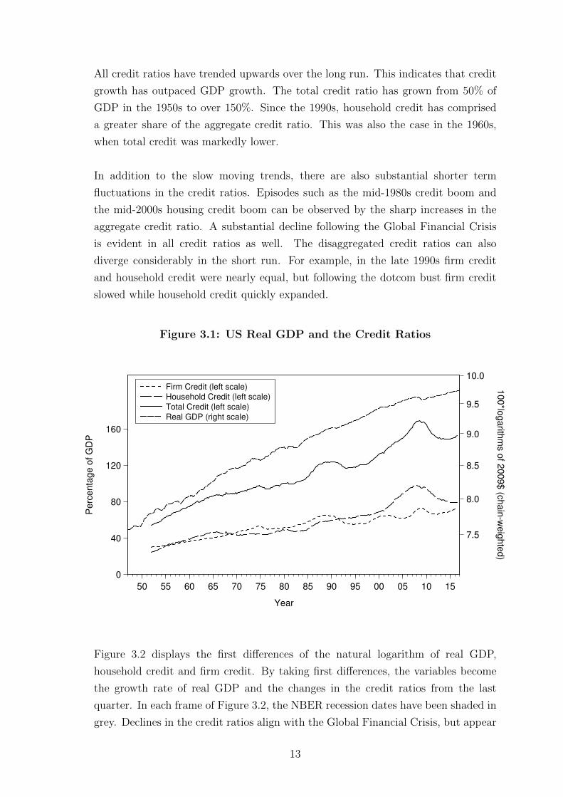
All credit ratios have trended upwards over the long run. This indicates that credit
growth has outpaced GDP growth. The total credit ratio has grown from 50% of
GDP in the 1950s to over 150%. Since the 1990s, household credit has comprised
a greater share of the aggregate credit ratio. This was also the case in the 1960s,
when total credit was markedly lower.
In addition to the slow moving trends, there are also substantial shorter term
fluctuations in the credit ratios. Episodes such as the mid-1980s credit boom and
the mid-2000s housing credit boom can be observed by the sharp increases in the
aggregate credit ratio. A substantial decline following the Global Financial Crisis
is evident in all credit ratios as well. The disaggregated credit ratios can also
diverge considerably in the short run. For example, in the late 1990s firm credit
and household credit were nearly equal, but following the dotcom bust firm credit
slowed while household credit quickly expanded.
Figure 3.1: US Real GDP and the Credit Ratios
0
40
80
120
160
10.0
9.5
9.0
8.5
8.0
7.5
50 55 60 65 70 75 80 85 90 95 00 05 10 15
Firm Credit (left scale)Household Credit (left scale)Total Credit (left scale)Real GDP (right scale)
Year
Perc
enta
ge o
f G
DP
100*lo
garith
ms o
f 2009$ (c
hain
-weig
hte
d)
Figure 3.2 displays the first differences of the natural logarithm of real GDP,
household credit and firm credit. By taking first differences, the variables become
the growth rate of real GDP and the changes in the credit ratios from the last
quarter. In each frame of Figure 3.2, the NBER recession dates have been shaded in
grey. Declines in the credit ratios align with the Global Financial Crisis, but appear
13

delayed or even unrelated during other recessions. For example, household credit
increases during the 2001 recession.
The focus of this analysis is the long run relationship between the credit ratios
and real GDP, displayed in Figure 3.1. Using a time series approach, I examine the
nature of the trends in these variables and how these trends may be related, if at all.
Specifically, I examine if the shocks that drive permanent movements in one variable
also drive permanent movements in another. The differenced variables presented in
Figure 3.2 are used in a VAR in Section 6.
Figure 3.2: US Real GDP Growth and Differenced Credit Ratios
-4
-2
0
2
4
1950 1960 1970 1980 1990 2000 2010
100* log difference of Real GDP
-2
-1
0
1
2
3
1950 1960 1970 1980 1990 2000 2010
D(Household Credit)
-2
-1
0
1
2
1950 1960 1970 1980 1990 2000 2010
D(Firm Credit)
14

Section 4
Cointegration Analysis
In this section I examine if a long run equilibrium relationship exists between
household credit, firm credit and real GDP in the United States. I first consider
whether the trend in each series is stochastic or deterministic. A trend is stochastic
if it is comprised of random shocks that have permanent effects on the conditional
mean of a series. If the permanent movements in household credit, firm credit and
real GDP are driven by the same stochastic trend, these variables are said to be
cointegrated. I investigate this possibility using the Engle-Granger and Johansen
tests. The results of these cointegration tests are mixed. Supposing these variables
are cointegrated I estimate a vector error correction model (VECM) and consider
the dynamic paths of each variable using impulse response functions.
4.1 Unit Root Tests
I formally test for stochastic trends using the Augmented Dickey-Fuller (ADF) test.
The ADF test considers whether a given series has a stochastic trend by testing for
the presence of a unit root (Enders, 2008, p. 215). Using the following regression, a
variable has a unit root if ρ− 1 = 0:
∆yt = α + βt+ (ρ− 1)yt−1 +
p∑i=2
∆yt−i+1 + εt (4.1)
To correct for serial correlation, p lags of the differenced variable are included. The
specific number of lags is chosen by minimising the Akaike information criterion
(AIC). Since each series trends upwards, the regression includes a constant and
time trend to improve the power of the test. Table 4.1 reports the ADF test results.
The selected number of lags indicates a large degree of persistence in the credit
ratios, particularly household credit. While too many lags will reduce the power of
the ADF test, too few lags will result in a serially correlated error term which will
bias the test. I follow the recommendation of Ng and Perron (1995) to include the
last lag if the absolute value of the t-statistic exceeds 1.6. The t-statistics of lags 4,
8, 12 and 14 for the coefficients of ∆ht were highly statistically significant.
15

Table 4.1: ADF Tests for Unit Roots
Variable Lags t-statistic p-valuea
Household Credit 14 -2.75 0.22
Firm Credit 10 -2.69 0.24
Total Credit 9 -3.40 0.05
Log Real GDP 1 -1.25 0.90a MacKinnon (1996) one-sided p-values
The ADF test cannot reject there is a unit root in the household and firm credit
ratios at the 5% level. This indicates that there are permanent movements in
the credit ratios overtime. These movements are random shocks with permanent
effects such as changes in regulation, the invention of new financial products or
improved productivity in the financial sector. The remainder of this thesis concerns
determining whether these shocks are also common to real GDP.
In addition to the ADF test, I test for stochastic trends using the ADF test with
generalised least squares detrending (ADF-GLS) as proposed by Elliott, Rothenberg,
and Stock (1996). This test has more power compared to the ADF test against near
unit root alternatives. I also complement these tests with the non-parametric KPSS
test (Kwiatkowski, Phillips, Schmidt, and Shin, 1992). Unlike the ADF test, the
KPSS test assumes that a series is trend stationary under the null hypothesis. The
results of the ADF-GLS and KPSS tests are presented in Table A.1 and Table A.2.
Collectively, the unit root tests indicate that the disaggregated credit ratios are first-
order integrated. This result implies that the aggregate credit ratio has a unit root
as it is the sum of two series with unit roots and these disaggregated components
are not cointegrated (see Table A.4). However, in isolation the unit root tests of the
aggregate credit ratio suggest it is trend-stationary. This seemingly contradictory
result possibly reflects that movements in household credit and firm credit have
historically been negatively correlated and retrospectively offset each other. It may
be indicative of a structural crowding-out effect, but considering the wide variety of
domestic and foreign lenders as well as financial instruments captured by the data,
crowding-out is less likely in the short term. Historically, one credit series may have
grown quickly for a short period while the other credit series declined, as occurred
in the late 1990s following the dotcom bust. This highlights a clear benefit of using
disaggregated data is greater power to detect stochastic trends.
16
The unit root tests clearly suggest real GDP has a unit root. I also conduct the ADF
test on the first differences of each series and find none to be second-order integrated
(see Table A.3). Since the disaggregated credit series are first-order integrated, there
now exists the potential for a cointegrating relationship, which may be modelled in
an error correction framework.
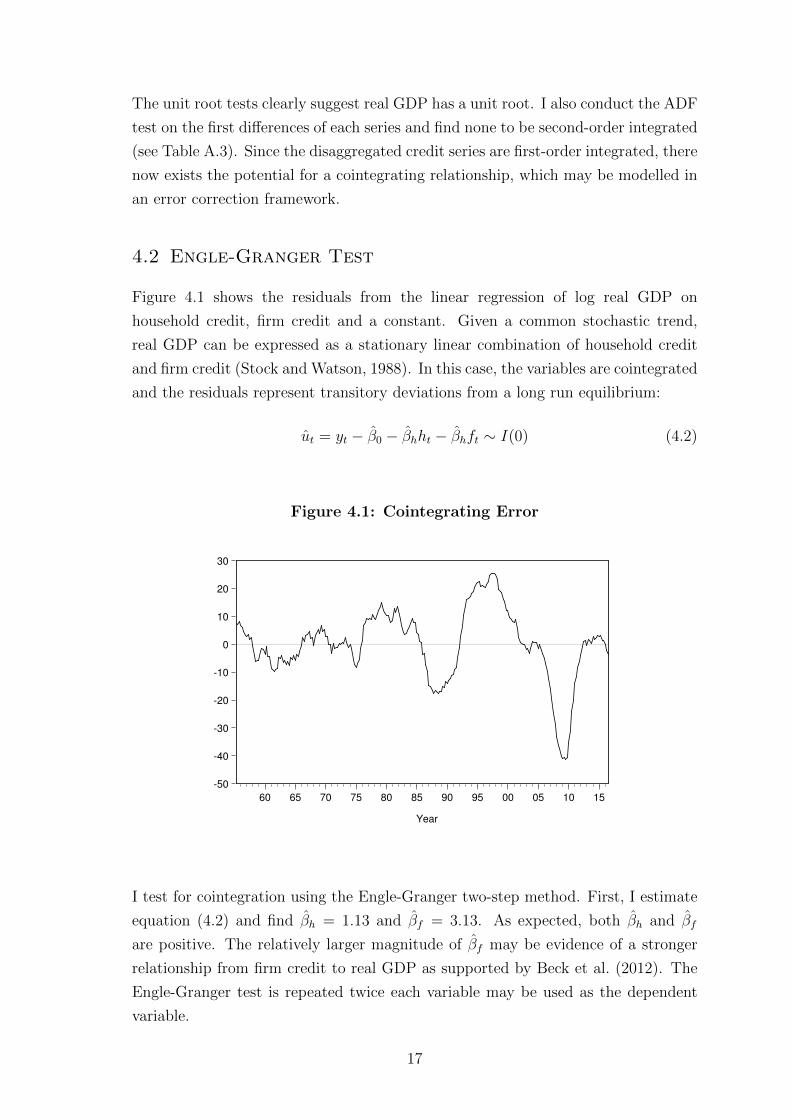
4.2 Engle-Granger Test
Figure 4.1 shows the residuals from the linear regression of log real GDP on
household credit, firm credit and a constant. Given a common stochastic trend,
real GDP can be expressed as a stationary linear combination of household credit
and firm credit (Stock and Watson, 1988). In this case, the variables are cointegrated
and the residuals represent transitory deviations from a long run equilibrium:
ut = yt − β0 − βhht − βhft ∼ I(0) (4.2)
Figure 4.1: Cointegrating Error
-50
-40
-30
-20
-10
0
10
20
30
60 65 70 75 80 85 90 95 00 05 10 15
Year
I test for cointegration using the Engle-Granger two-step method. First, I estimate
equation (4.2) and find βh = 1.13 and βf = 3.13. As expected, both βh and βf
are positive. The relatively larger magnitude of βf may be evidence of a stronger
relationship from firm credit to real GDP as supported by Beck et al. (2012). The
Engle-Granger test is repeated twice each variable may be used as the dependent
variable.
17

To produce asymptotically efficient estimates as well as asymptotically normal t-
statistics, the cointegrating equation can also be estimated by a dynamic ordinary
least squares (DOLS) regression (Stock and Watson, 1993). This is done by including
a sufficient number of leads and lags of the differenced independent variables to
remove long run correlation between the variables. Using real GDP as the dependent
variable, the AIC and Schwarz information criterion (SIC) suggest a substantial
number of leads and lags. Using 12 lags and 12 leads βh = 1.10 and βf = 3.36.
The second step is to test if the residuals are stationary using the ADF test. Since
all variables drift upwards, the ADF test includes a linear deterministic trend. Lag
selection of ∆ut is based on the AIC criterion. The Engle-Granger tau statistics and
p-values are presented in Table 4.2
Table 4.2: Engle-Granger Test with Disaggregated Credit Ratios
Dependent Variable Lags tau-statistic p-valuea
Log Real GDP 8 -3.82 0.05
Household Credit 14 -2.57 0.48
Firm Credit 8 -3.92 0.04a MacKinnon (1996) p-values
The null hypothesis of no cointegration is rejected when using real GDP or firm
credit as the dependent variable since the residuals are found to be stationary at
the 5% level. Ideally the residuals should be stationary irrespective of the choice
of variable for normalisation. The failure to reject no cointegration when using
household credit as the dependent variable may indicate that household credit is
being driven by a separate stochastic trend. Overall, the Engle-Granger test lends
some support to a cointegrating relationship between real GDP, household credit
and firm credit.
Table 4.3 reports the Engle-Granger test results for a cointegrating relationship
between the aggregate credit ratio and real GDP. When using the aggregate
credit ratio instead of its disaggregated components, the residuals are found to be
stationary at a 10% level rather than a 5% level. Since the Engle-Granger test offers
weaker evidence of a long run relationship when using the aggregate credit ratio, it
seems there is more potential to discover possible cointegrating relationships using
disaggregated credit ratios.
18

Table 4.3: Engle-Granger Test with Aggregate Credit Ratio
Dependent Variable Lags tau-statistic p-valuea
Log Real GDP 8 -3.26 0.08
Total Credit 8 -3.35 0.06a MacKinnon (1996) p-values
4.3 Johansen Test
To further test for cointegration I conduct Johansen tests. A benefit of the Johansen
test is the ability to test for and estimate multiple cointegrating vectors (Enders,
2008, p. 385). Since there are three variables, there may be as many as two
cointegrating vectors which implies each bivariate pairing is cointegrated.
It is assumed the nonstationary variables have a VAR(p) representation, and there
is a linear combination of these variables such that the error term is stationary.
The Johansen approach follows from the error correction representation of the
nonstationary variables given by:
∆xt = µ+ π∗x∗t−1 +
p−1∑i=1
Γi∆xt−i + εt (4.3)
where ∆xt is a (3×1) vector of first differences(
∆yt ∆ht ∆ft
)′, µ is a (3×1) vector
of constants, π∗ is a (4× 4) matrix of coefficients, x∗t−1 =(yt−1 ht−1 ft−1 1
)′, Γi
are (i × 3) coefficient matrices and εt is a vector of independently and identically
distributed disturbance terms.
The term π∗x∗t−1 is the error correction term. The rank of π∗ corresponds to the
number of cointegrating vectors. The eigenvalues of π∗ are estimated by maximum
likelihood estimation, and it is the number of non-zero eigenvalues that determine
the rank of π∗. If the rank of π∗ is zero, there is no cointegration and the model
becomes a VAR of the first differences. If π∗ is full rank this implies the variables
are stationary. The variables are cointegrated if the rank of π∗ is equal to 1 or 2.
The maximum eigenvalue and trace statistic tests determine the number of distinct
cointegrating vectors. Including µ allows for linear times trends so the rank of π∗
19

reflects the number of cointegrating vectors in the detrended data.3
I allow for an intercept in the cointegrating equation and a linear deterministic trend
in the VAR as seen in equation (4.3). To determine lag length, I estimate a VAR of
the undifferenced variables. Based on this VAR, the SIC selects p = 5, AIC selects
p = 9, and the Likelihood Ratio (LR) test selects p = 13. Table 4.4 presents the
trace test and max eigenvalue tests for each of these selections, where p− 1 lags of
the differenced variables are used.
The Johansen approach is much less supportive of cointegration compared to the
Engle-Granger approach. The results of the trace test and max eigenvalue test are
often at odds, and are not robust to the number of lagged differenced variables.
Depending on the choice of lag length, the trace statistic indicates there may be
two cointegrating vectors. This is unlikely since it implies each bivariate pair is
cointegrated and I find no evidence that household and firm credit are cointegrated
(see Table A.4). At all lag lengths, the max eigenvalue statistic does not support
one cointegrating vector at a 5% level.
4.4 VECM Analysis
Overall the results for cointegration are mixed. The maximum eigenvalue test
statistic suggests no cointegration while the Engle-Granger test lends support to
cointegration.
Supposing there is in fact cointegration, the VECM provides a means of representing
the long run relationship between real GDP and the two credit ratios. If it is assumed
there is one cointegrating vector, π∗ can be rewritten as αβ′ and the relationship
between the variables described by:
∆xt = µ+ α(β′x∗t−1) +
p−1∑i=1
Γi∆xt−i + εt (4.4)
where αβ′x∗t−1 =
αyαhαf
[1 −βh −βf −β0]yt−1
ht−1
ft−1
1
(4.5)
β is the cointegrating vector, such that β′xt−1 is a linear stationary process, and
3The intercept in the cointegrating vector is not separately identified from µ. EViews identifiesβ0 as the value required for the error correction term to have mean of zero
20

Table 4.4: Johansen Tests
Null hypothesis Alternative hypothesis 95% critical value p-value a
p = 5
λtrace tests λtrace value
r = 0 r > 0 34.52 29.80 0.01
r ≤ 1 r > 1 13.69 15.49 0.09
λmax tests λmax value
r = 0 r = 1 20.83 21.13 0.06
r = 1 r = 2 12.00 14.26 0.11
p = 9
λtrace tests λtrace value
r = 0 r > 0 33.64 29.80 0.02
r ≤ 1 r > 1 16.30 15.49 0.04
λmax tests λmax value
r = 0 r = 1 17.34 21.13 0.16
r = 1 r = 2 9.76 14.26 0.23
p = 13
λtrace tests λtrace value
r = 0 r > 0 26.65 29.80 0.11
r ≤ 1 r > 1 12.95 15.49 0.12
λmax tests λmax value
r = 0 r = 1 13.70 21.13 0.39
r = 1 r = 2 7.48 14.26 0.43a MacKinnon, Haug, and Michelis (1999) p-values
the elements of α are the error correction coefficients. The magnitude of the error
correction coefficients indicates the predicted adjustment of the variables to long
run equilibrium in each quarter. The Γi coefficients on the lags of the differenced
variables can be interpreted as the short run effects (see Table A.5).
I estimate the VECM with twelve lags of the differenced variables to remove the
serial correlation. Table 4.5 reports the error correction coefficients and cointegrating
vector, where the coefficient on real GDP is normalised to one. Since yt is 100 times
the natural logarithm of real GDP, the error correction coefficients are small in size
and therefore reported as percentages.
21

Table 4.5: VECM Estimates
Cointegrating equation β0 βh βf
641.46 1.42 3.06
(s.e.) (0.33) (0.53)
Dependent Variable α (%) R2
∆ Log Real GDP 0.09 0.25
(s.e.) (0.57)
∆ Household Credit 0.89 0.65
(s.e.) (0.30)
∆ Firm Credit 0.36 0.69
(s.e.) (0.20)
The crucial implication of the VECM results is that the error correction coefficient
for real GDP is not statistically different from zero. This indicates that real GDP is
weakly exogenous. In a cointegrated system, real GDP does not adjust in response
to changes in the credit ratios, that is, permanent movements in the credit ratios do
not drive output. Although the error correction term αy should be negative since
the coefficient on real GDP is normalised to one, the error correction mechanism
functions as all the adjustment to long run equilibrium is done by the credit ratios
in response to changes in real GDP.
Finding real GDP is weakly exogenous places these results at odds with the
Schumperterian view of the finance-growth relationship. It is also at odds with
most cross-country studies that find a this relationship is bi-directional. These
results may simply reflect a degree of country heterogeneity exists, particularly when
comparing advanced and developing countries. Another explanation for finding
weakly exogenous real GDP may be that real GDP is very slow to respond to
permanent movements in the credit ratios. The test for weak exogeneity has low
power to detect a slow moving endogenous variable, so real GDP might not actually
be weakly exogenous (see Morley, 2007).
Since real GDP appears to be weakly exogenous, I estimate the cointegrating vector
by DOLS with firm credit as the dependent variable. Using AIC, the equation is
estimated with no leads and three lags, as well as HAC standard errors. The reported
coefficients on household credit and real GDP are βh = −0.11 and βy = 0.23, both of
22
which are statistically significant. The negative estimate of βh reflects the historical
offsetting between the credit ratios, while the positive estimate of βy suggests real
GDP has positive permanent effects on firm credit.
The estimates of αh and αf suggest most of the adjustment is done by household
credit rather than firm credit. If correct, this indicates household borrowing is
more responsive to changes in output. At the same time, the magnitude of the
coefficients from the cointegrating vector suggest the long run relationship with real
GDP is stronger with firm credit. To test if household credit should be included in
the cointegrating vector, I restrict βh to zero. The corresponding likelihood ratio
statistic is 4.81, so the null hypothesis is rejected at a 5% level.
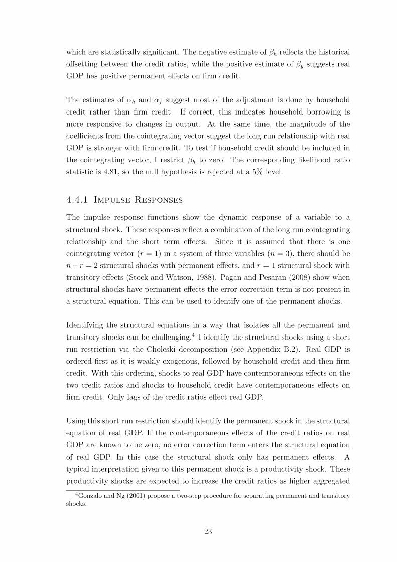
4.4.1 Impulse Responses
The impulse response functions show the dynamic response of a variable to a
structural shock. These responses reflect a combination of the long run cointegrating
relationship and the short term effects. Since it is assumed that there is one
cointegrating vector (r = 1) in a system of three variables (n = 3), there should be
n− r = 2 structural shocks with permanent effects, and r = 1 structural shock with
transitory effects (Stock and Watson, 1988). Pagan and Pesaran (2008) show when
structural shocks have permanent effects the error correction term is not present in
a structural equation. This can be used to identify one of the permanent shocks.
Identifying the structural equations in a way that isolates all the permanent and
transitory shocks can be challenging.4 I identify the structural shocks using a short
run restriction via the Choleski decomposition (see Appendix B.2). Real GDP is
ordered first as it is weakly exogenous, followed by household credit and then firm
credit. With this ordering, shocks to real GDP have contemporaneous effects on the
two credit ratios and shocks to household credit have contemporaneous effects on
firm credit. Only lags of the credit ratios effect real GDP.
Using this short run restriction should identify the permanent shock in the structural
equation of real GDP. If the contemporaneous effects of the credit ratios on real
GDP are known to be zero, no error correction term enters the structural equation
of real GDP. In this case the structural shock only has permanent effects. A
typical interpretation given to this permanent shock is a productivity shock. These
productivity shocks are expected to increase the credit ratios as higher aggregated
4Gonzalo and Ng (2001) propose a two-step procedure for separating permanent and transitoryshocks.
23

income encourages more borrowing.
The short run restriction forces the structural shocks to be uncorrelated but does not
isolate the remaining permanent and transitory shocks. The error correction term is
present in the structural equations of both the credit ratios so the impulse responses
capture transitory and permanent effects to a structural shock. The remaining
permanent shock may be a credit supply shock. A credit supply shock indicates lower
credit constraints which should increase investment and drive economic growth.
Determining the transitory structural shock is more difficult. One interpretation
may be a risk aversion shock, since perceptions of risk will affect sentiments to
borrow and lend. This is the interpretation given to a transitory shock by Lettau
and Ludvigson (2014) in a VECM consisting of consumer spending, labour earnings
and asset wealth. A simpler interpretation may be monetary policy shocks, since
changes in the real interest rate effects demand for credit and has transitory effects
on output.
Figure 4.2 shows the impulse responses to a one standard deviation exogenous
structural shock. The first column shows the impulse response of each variable to
a ‘productivity’ shock. Real GDP has a permanent response as it is nonstationary.
Firm credit appears to have a permanent positive response and household credit no
response. The second and third columns show the impulse responses of each variable
to a shock in the structural equations of household and firm credit. A shock in the
structural equation of a credit ratio has a positive permanent effect on the credit
ratio itself and a negative permanent effect on the other credit ratio. A shock to the
structural equation of household credit has a positive transitory effect on real GDP
and oddly a shock to the structural equation of firm credit has a negative effect on
real GDP.
To some degree these responses reflect that imposing cointegration on real GDP,
household credit and firm credit requires there should be two permanent structural
shocks and one transitory shock. Considering the mixed cointegration test results,
it may be that these impulse responses do not reflect the true dynamic responses.
Identifying the structural shocks also assumes that the short run restriction was
appropriate. This raises the need to re-evaluate if these variables are cointegrated
and find another approach to identify permanent shocks.
24
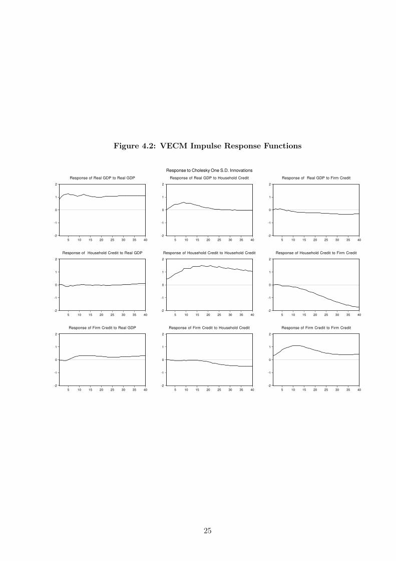
Figure 4.2: VECM Impulse Response Functions
-2
-1
0
1
2
5 10 15 20 25 30 35 40
Response of Real GDP to Real GDP
-2
-1
0
1
2
5 10 15 20 25 30 35 40
Response of Real GDP to Household Credit
-2
-1
0
1
2
5 10 15 20 25 30 35 40
Response of Real GDP to Firm Credit
-2
-1
0
1
2
5 10 15 20 25 30 35 40
Response of Household Credit to Real GDP
-2
-1
0
1
2
5 10 15 20 25 30 35 40
Response of Household Credit to Household Credit
-2
-1
0
1
2
5 10 15 20 25 30 35 40
Response of Household Credit to Firm Credit
-2
-1
0
1
2
5 10 15 20 25 30 35 40
Response of Firm Credit to Real GDP
-2
-1
0
1
2
5 10 15 20 25 30 35 40
Response of Firm Credit to Household Credit
-2
-1
0
1
2
5 10 15 20 25 30 35 40
Response of Firm Credit to Firm Credit
Response to Cholesky One S.D. Innovations
25
Section 5
Unobserved Components Model
The initial time series analysis of real GDP, household credit and firm credit raises
several questions of interest. Are these variables truly cointegrated? Is real GDP
actually weakly exogenous? Do credit ratios play any role driving real GDP in the
long run? To answer these questions and verify the results of the cointegration
analysis I apply the data to a correlated unobserved components model.
The unobserved components model proposed by Harvey (1985), provides a means to
decompose a series into its permanent (stochastic trend) component and a transitory
(stationary) component. The permanent component follows a random walk plus
drift, and the transitory component follows a stationary and invertible ARMA(p, q)
process. The permanent and transitory shocks that form each component are
distinct but unobservable. Morley, Nelson, and Zivot (2003) show these two distinct
shocks can be identified while being contemporaneously correlated with each other.
I estimate a multivariate unobserved components model of real GDP, household
credit and firm credit, allowing for correlation between the permanent and transitory
movements within a given series as well as across series.
Using this model addresses some of the limitations of the VECM. One clear
finding from the cointegration analysis was the high degree of persistence in the
credit ratios, particularly household credit. The VECM required a substantial
number of lags to account for serial correlation. Expressing each variable in
terms of transitory and permanent shocks instead may provide a more appropriate
model specification. It can be shown that every VECM has an equivalent
unobserved components model with a reduced-form vector autoregressive moving-
average (VARMA) representation (Schleicher, 2003). Since a moving average process
inverts to an infinite order autoregressive process, an unobserved components model
provides a more parsimonious approach to capture the dynamics in the data.
The distinct advantage of using the unobserved components model is the identifica-
tion of permanent shocks. To establish a long run relationship between output and
credit ratios in the data it is necessary to discern between permanent and transitory
shocks. A long run relationship exists if the permanent shock in one variable causes
26
a permanent shock to another variable. The structural shocks recovered in a VECM
or VAR are sensitive to the choice of identification strategy and as a result may be
either transitory or permanent shocks, or combine the effect of both. To verify the
cointegration tests and VECM results I first construct an unobserved components
model with a single stochastic trend that is common to real GDP, household credit
and firm credit. I later develop an unobserved components model with multiple
stochastic trends to examine if there is any commonality between the permanent
movements in real GDP and the credit ratios. This model is designed so that the
ordering of the variables determines which variable has permanent effects on another
and is used to investigate the VECM finding that real GDP is weakly exogenous.
Another way to investigate the direction of causality is to examine the speed the
variables adjust. One alternate explanation to real GDP being weakly exogenous is
that it adjusts very slowly overtime. The VECM may give the illusion real GDP is
weakly exogenous if the model has low power to detect a slow moving endogenous
variable. One of the limitations of the VECM is that the error correction term
implies all variables adjust back to their long run equilibrium levels at the same
speed. The exception is if a variable is weakly exogenous. A weakly exogenous
variable adjusts instantaneously as it does not respond to the other variables. The
unobserved components model allows each variable to adjust at different speeds to
long run equilibrium.
Following from Morley (2007), I measure the speed of adjustment by the half-life
response of a variable to a shock. In this thesis the term speed of adjustment is used
in the context of the unobserved components model and not to refer to the error
correction coefficients in the VECM. The speed of adjustment captures the amount
of time a variable takes to adjust to a new long run level. In contrast, the VECM
error correction coefficients capture the expected size of adjustment in each period.
A slow moving variable which needs more time to reach a new long run level, is
less likely to have permanent effects on a faster moving variable. This follows from
the rationale of Granger causality. If the past movements of one variable forecasts
future movements in another, it must adjust in time to do so. Supposing credit
ratios drives permanent movements in real GDP, the credit ratios should adjust first
which then effects real GDP, rather than real GDP adjusting instantaneously. If
real GDP adjusts very slowly, it may be the credit ratios that are weakly exogenous.
The unobserved components model also estimates correlations between the per-
manent and transitory components. These correlations can be used to explain
27

the dynamics of real GDP, household credit and firm credit. For example, in an
unobserved components model of US output and unemployment, Sinclair (2009)
finds a negative correlation between their permanent components, as well as a
negative correlation between the permanent and transitory shocks within both series.
A negative correlation between the permanent and transitory component within a
series indicates a partial adjustment to a new long run level over time. Morley
et al. (2003) estimate a correlation of -0.91 between the permanent and transitory
component of US GDP in a univariate unobserved components model. A typical
interpretation given to this correlation is the ‘time to build’ effects of Kydland and
Prescott (1982). Since it takes multiple time periods to build new capital goods,
the transitory component of real GDP lags behind a permanent shock. I interpret
the correlations in the unobserved components model as the effect of a permanent
shock on the transitory adjustment of a variable to a new long run level.
5.1 Unobserved Components Model for Cointegration
To begin, I re-examine whether it is appropriate to impose cointegration on real
GDP, household credit and firm credit. The following model is based on a correlated
unobserved components model for cointegration of income and consumption from
Morley (2007). I now extend the model to three variables.
Real GDP (y), household credit (h) and firm credit (f) are each decomposed into
an unobservable permanent component and transitory component:
yt = τt + uyt (5.1)
ht = h+ γτt + uht (5.2)
ft = f + λτt + uft (5.3)
where τt is the permanent component, uyt is the transitory component of real
GDP, uht is the transitory component of household credit and uft is the transitory
component of firm credit. The parameters γ and λ relate each variable to the
permanent component and the intercepts h and f reflect the long run effect of other
factors on the level of the credit ratios, such as regulations.
The permanent component is a stochastic trend and is assumed to be common to
each variable. It follows a random walk with drift µ to capture the long term upward
drift of all three variables:
τt = µ+ τt−1 + vt (5.4)
28

where vt ∼ i.i.d.N(0, σ2v). It is assumed that each unobservable transitory
component is stationary and follows an autoregressive process of order two (AR(2)):
uyt − φy,1uy,t−1 − φy,2uy,t−2 = εyt (5.5)
uht − φh,1uh,t−1 − φh,2uh,t−2 = εht (5.6)
uft − φf,1uf,t−1 − φf,2uf,t−2 = εft (5.7)
where εit ∼ i.i.d.N(0, σ2i ) and φi,0 is normalised to one for i = y, h, f . Finally, it is
assumed that the permanent shocks (vt) and each of the transitory shocks (εit) are
correlated with each other.
ρyh = corr(εyt, εht) (5.8)
ρyf = corr(εyt, εft) (5.9)
ρyv = corr(vt, εyt) (5.10)
ρhf = corr(εht, εft) (5.11)
ρhv = corr(vt, εht) (5.12)
ρfv = corr(vt, εft) (5.13)
By imposing a common stochastic trend, this unobserved components model should
mirror the results of the VECM. There is one cointegrating vector and therefore two
types of permanent shocks. I interpret the shocks to the permanent component vt,
as being either productivity shocks to yt or credit shocks to ht and ft which drive all
variables. Consider the cointegrating vector of the VECM. It is a stationary linear
combination of the variables and a constant, where the coefficient of yt is normalised
to one.
E
1
−βh−βf−β0
[yt ht ft 1
]= 0 ∼ I(0)
The parameters γ and λ as well as the intercept terms h and f link the unobserved
components model to the cointegrating vector. This can be shown by substituting τt
from equation (5.1) into equations (5.2) and (5.3) and then summing them together
so that:
yt −1
2γht −
1
2λft +
1
2γh+
1
2λf = uyt −
1
2γuht −
1
2λuft ∼ I(0)
The transitory components are assumed to be normally distributed and have a mean
of zero, so the left hand side is analogous to the cointegrating vector. It is anticipated
that βh ≈ 12γ
, βf ≈ 12λ
and the constant −β0 ≈ 12γh+ 1
2λf .
29
This unobserved components model does not have an explicit error correction
mechanism like the VECM. Instead, the long run relationship between the variables
is indicated by the parameter estimates of γ and λ. The correlations with vt
reflect transitory effects. If a common stochastic trend is an appropriate model,
the transitory components should be stationary and the parameter estimates of γ
and λ statistically significant.
5.1.1 Estimation
To estimate the unobserved components model given by equations (5.1) to (5.13),
I rewrite the model in state-space form. Once in state-space form, maximum
likelihood estimates of the parameters are obtained using the Kalman filter and
the prediction error decomposition.
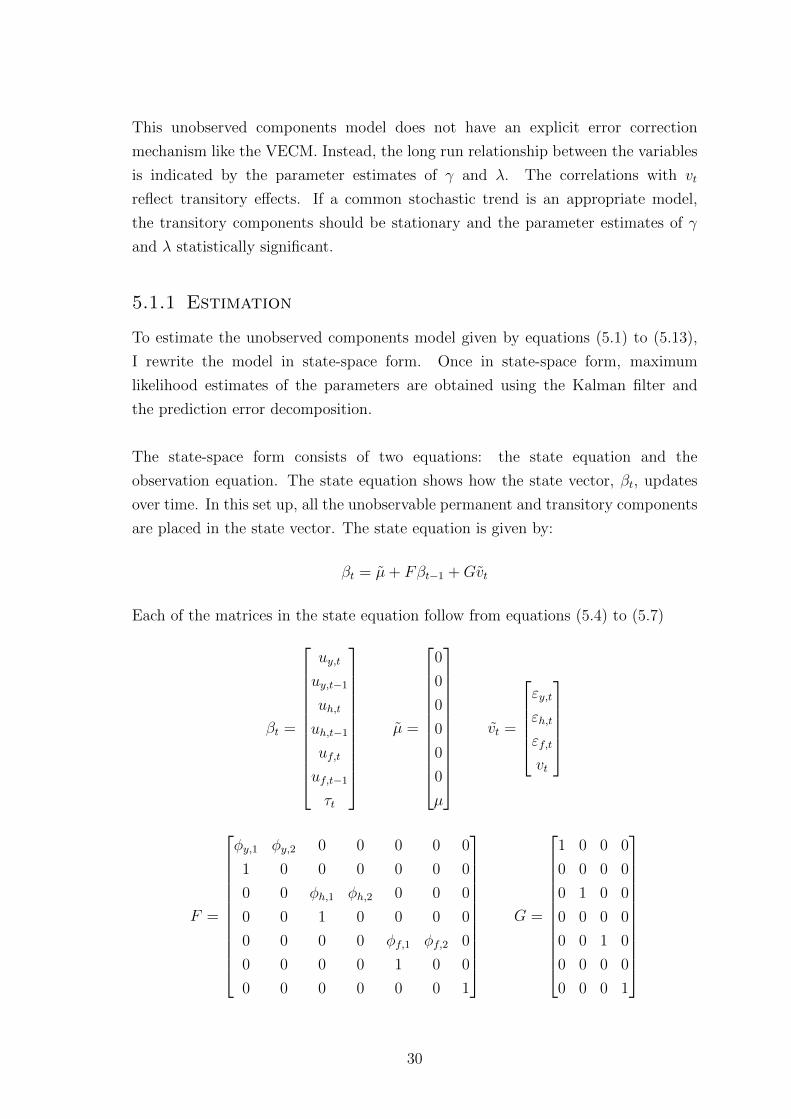
The state-space form consists of two equations: the state equation and the
observation equation. The state equation shows how the state vector, βt, updates
over time. In this set up, all the unobservable permanent and transitory components
are placed in the state vector. The state equation is given by:
βt = µ+ Fβt−1 +Gvt
Each of the matrices in the state equation follow from equations (5.4) to (5.7)
βt =
uy,t
uy,t−1
uh,t
uh,t−1
uf,t
uf,t−1
τt
µ =
0
0
0
0
0
0
µ
vt =
εy,t
εh,t
εf,t
vt
F =
φy,1 φy,2 0 0 0 0 0
1 0 0 0 0 0 0
0 0 φh,1 φh,2 0 0 0
0 0 1 0 0 0 0
0 0 0 0 φf,1 φf,2 0
0 0 0 0 1 0 0
0 0 0 0 0 0 1
G =
1 0 0 0
0 0 0 0
0 1 0 0
0 0 0 0
0 0 1 0
0 0 0 0
0 0 0 1
30

The covariance matrix for vt follows from model equations (5.8) to (5.13), and is
denoted by Q:
Q =
σ2y ρyhσyσh ρyfσyσf ρyvσyσv
ρyhσyσh σ2h ρhfσhσf ρhvσhσv
ρyfσyσf ρhfσhσf σ2f ρfvσfσv
ρyvσyσv ρhvσhσv ρfvσfσv σ2v
The observation equation relates the observable data to the state vector. The
observation equation is given by:
yt = A+Hβt
This follows from equations (5.1) to (5.3) where:
yt =
ythtft
A =
0
h
f
H =
1 0 0 0 0 0 1
0 0 1 0 0 0 γ
0 0 0 0 1 0 λ
Once the unobserved components model is expressed in state-space form, the
Kalman filter estimates the minimum mean squared error estimate of the state
vector βt (Kim and Nelson, 1999). The Kalman filter comprises of the following six
recursive equations:
βt|t−1 = µ+ Fβt−1|t−1
Pt|t−1 = FPt−1|t−1F′ +GQG′
ζt|t−1 = yt −Hβt|t−1
ψt|t−1 = HPt|t−1H′
βt|t = βt|t−1 +Ktζt|t−1
Pt|t = Pt|t−1 −KtHPt|t−1
The first two equations of the Kalman filter describe the prediction of βt using
information up to time t−1 and assuming µ, F , and Q are known. At the beginning
of time t, βt|t−1, the expectation of βt conditional on information up to time t − 1,
is calculated. Also calculated is Pt|t−1, the covariance matrix of βt|t−1.
ζt|t−1 is the conditional prediction error of the observable data and ψt|t−1 is the
covariance matrix of ζt|t−1. Hβt|t−1 gives the optimal prediction of yt|t−1 from which
the prediction error is calculated at the end of time t. This prediction error captures
new information about βt which is then used to update the state vector and the
31
corresponding covariance matrix as seen in the last two equations of the Kalman
filter. Kt = Pt|t−1H′ψ−1t|t−1 is the weight given to new information in the prediction
error, known as the Kalman gain.
Initial values β0|0 and P0|0 are required to iterate the six equations of the Kalman
filter for t = 1, 2, ..., T . While the first six elements of βt are the transitory
components and assumed to be stationary with mean zero, the final element τt
is nonstationary so the unconditional mean does not exist. I set τ0|0 = 779.3, which
is the first data point of 100 times the natural logarithm of real GDP. I set the final
element of the corresponding covariance matrix, var(τ0|0) = 100. In each unobserved
components model I check the parameters estimates are robust to other values of
var(τ0|0).
The maximum likelihood estimates of the parameters use the prediction errors
(ζt|t−1) and variances (ψt|t−1) from the Kalman filter.5 This follows from the
prediction error decomposition of the log likelihood function shown by Harvey
(1993):
ln(θ) = −1
2
T∑t=2
ln((2π)2ψt|t−1) −1
2
T∑t=2
ln(ζ ′t|t−1ψ−1t|t−1ζt|t−1)
where θ is the parameter vector. Since the dependent variables of the VECM are
differenced, I evaluate the log likelihood from observation two, rather than the first
observation so the sample periods are the same. Generally, the starting observation
should be large enough to minimise the effect of the arbitrary initial values chosen
for β0|0 and P0|0 (Kim and Nelson, 1999).
The parameters are constrained so the variance-covariances matrix Q is positive
definite and the auto-regressive parameters of the transitory components are
stationary.
5.1.2 Identification
In the VECM, short run restrictions were imposed to identify the structural shocks.
The unobserved components model makes no such restrictions to recover the
stochastic trend and transitory shocks. Instead, the necessary requirement is to
allow for sufficient model dynamics in the transitory components. Traditionally,
the permanent and transitory shocks were recovered by assuming zero correlation
between these components. However, using US real GDP, Morley et al. (2003)
5Maximum likelihood estimation was done in Matlab using the numerical optimisation functionfminunc. The fminunc default settings were modified to allow for 10000 function evaluations.
32

showed that the stochastic trend shocks can be correlated with the transitory shocks
and can be econometrically identified so long as the transitory components have at
least second-order autoregressive dynamics.
Trenkler and Weber (2016) provide order and rank conditions for the identification
of multivariate correlated unobserved components models. For the order condition
to be satisfied, the number of parameters in the equivalent reduced form VARMA
model must be greater than the number of parameters in the structural unobserved
components model. This order condition holds given the transitory components
follow an autoregressive process of at least order two. The rank condition requires
the diagonal VAR(p) matrix that describes the transitory components to be full
rank. The rank condition is also satisfied if each of the transitory components
follow at least an second-order autoregressive process.
5.1.3 Results
Table 5.1 reports the parameter estimates and standard errors of the unobserved
components model for cointegration. The log likelihood of this model is -411.70.
The conclusion from the estimates of the transitory components is that the model is
misspecified. The AR(2) parameters of transitory household credit and firm credit
sum to one, or are very close to one. This indicates that the transitory components
are nonstationary. If the transitory components of household credit and firm credit
are nonstationary then there is at least one omitted stochastic trend.
This is evident from the hump-shaped impulse response functions seen in Figure 5.1.
The impulse response functions indicate the speed of adjustment of the variables.
At face value, the half-life of a shock to transitory real GDP is approximately
two quarters, whereas it is over thirty quarters for firm credit and even higher for
household credit. Since the transitory components of household and firm credit are
extremely persistent and possibly contain a unit root, these transitory components
have not been properly identified.
Interpreting the parameter estimates may be misleading since the credit ratios have
not been properly decomposed. While the credit ratios appear to adjust very slowly,
this is insufficient evidence to verify that real GDP is weakly exogenous as there is
likely a unit root in what is labelled as the transitory component of the credit
ratios. The cross-series correlations are also likely to be misleading. Although, since
real GDP was effectively decomposed into its components, the correlation between
transitory and permanent real GDP, ρyv, is very close to the estimate of -0.91 from
33

Table 5.1: Unobserved Components Model for Cointegration
Transitory Component Parameters
φy1 φy2 φh1 φh2 φf1 φf2
0.74 -0.08 1.96 -0.96 1.49 -0.51
(0.05) (0.03) (0.02) (0.02) (0.05) (0.05)
Variance Parameters
σy σh σf σv
1.55 0.13 0.47 1.50
(0.10) (0.02) (0.03) (0.11)
Permanent Component Parameters
µ h f γ λ
0.80 -231.76 -108.27 0.33 0.18
(0.09) (14.90) (12.30) (0.02) (0.01)
Correlation Parameters
ρyv ρhv ρfv ρhf ρyh ρyf
-0.92 0.27 -0.57 -0.10 0.12 0.47
(0.01) (0.21) (0.06) (0.17) (0.21) (0.06)
Morley et al. (2003). These estimates also vary from the VECM estimates βh = 1.42,
βf = 3.06 and −β0 = −641.46. The estimates of λ, γ, h and f correspond to
βh = 1.52, βf = 2.78 and −β0 = −651.90. These estimates of the cointegrating
vector can be replicated by DOLS using 30 lags and 20 leads.
5.1.4 Unobserved Components Model with 2 Stochastic
Trends
The apparent unit root in the transitory components of household and firm credit
indicates these credit ratios and real GDP do not simply share a single common
stochastic trend. To better identify the transitory adjustment of household and firm
credit, I extend the cointegration model to allow for two stochastic trends.
The first trend, τt drives all three variables and may be interpreted as either
productivity shocks or credit shocks depending on the direction of causation. The
second trend κt is another series of permanent credit shocks which drives only the
34
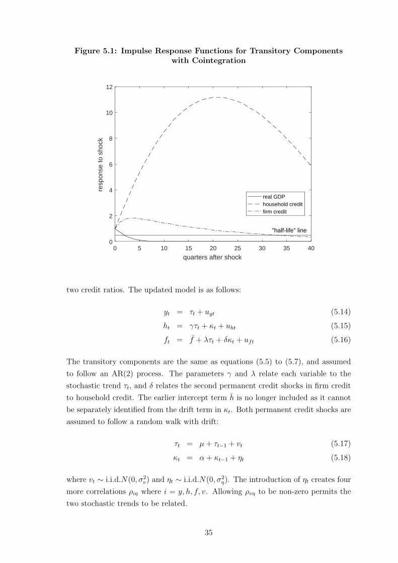
Figure 5.1: Impulse Response Functions for Transitory Componentswith Cointegration
0 5 10 15 20 25 30 35 40
quarters after shock
0
2
4
6
8
10
12
resp
onse
to s
hock
"half-life" line
real GDPhousehold creditfirm credit
two credit ratios. The updated model is as follows:
yt = τt + uyt (5.14)
ht = γτt + κt + uht (5.15)
ft = f + λτt + δκt + uft (5.16)
The transitory components are the same as equations (5.5) to (5.7), and assumed
to follow an AR(2) process. The parameters γ and λ relate each variable to the
stochastic trend τt, and δ relates the second permanent credit shocks in firm credit
to household credit. The earlier intercept term h is no longer included as it cannot
be separately identified from the drift term in κt. Both permanent credit shocks are
assumed to follow a random walk with drift:
τt = µ+ τt−1 + vt (5.17)
κt = α + κt−1 + ηt (5.18)
where vt ∼ i.i.d.N(0, σ2v) and ηt ∼ i.i.d.N(0, σ2
η). The introduction of ηt creates four
more correlations ρiη where i = y, h, f, v. Allowing ρvη to be non-zero permits the
two stochastic trends to be related.
35
The model is estimated using the Kalman filter. To ensure that the estimated
parameters are directly related to the estimates of the initial unobserved components
model, I set the initial estimate τ0|0 to 779.3, and for κ0|0 I set the initial value to
h = −231. Due to the large degree of uncertainty around these initial estimates, I
set var(τ0|0) and var(κ0|0) to 500.
The parameters estimates are shown in the Table 5.2. The log likelihood for this
model is -382.21. Despite controlling for an additional stochastic trend in the
credit ratios, the immediate finding is that the auto-regressive parameters for the
transitory component of firm credit nearly sum to one. This indicates that the
transitory component of firm credit is probably nonstationary. If allowing for two
stochastic trends was not sufficient to identify the transitory components, this is a
clear rejection of cointegration between real GDP, household credit and firm credit.
If the model is misspecified the parameter estimates of γ, λ and δ may be misleading.
The correlation estimates indicate that the second stochastic trend captures
important dynamics in household credit. There are strong correlations between the
permanent and transitory components within household credit and real GDP. In
household credit, ρhη is nearly -1. The relatively large variance ση shows permanent
movements in household credit are highly variable. Introducing a second stochastic
trend also resulted in low correlations between the components household credit and
real GDP, ρhv, ρyh, ρyη and ρvη.
Allowing for a third stochastic trend to properly identify the transitory and
permanent shocks of firm credit may also result in very different parameter estimates.
Since real GDP, household credit and firm credit each require separate stochastic
trends to capture all permanent movements, this brings into question whether any
long run relationship exists despite the supportive finding of the Engle-Granger test.
5.2 Unobserved Components Model with 3 Stochastic
Trends
While real GDP and the credit ratios do not appear to be cointegrated, there
may be some commonality between their permanent components. The unobserved
components model for cointegration imposed that the permanent components of
real GDP, household credit and firm credit were perfectly correlated. In this final
unobserved components model, each variable has a different permanent component.
These differing permanent components are allowed to be correlated with each other
36
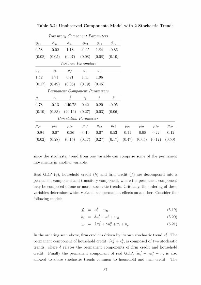
Table 5.2: Unobserved Components Model with 2 Stochastic Trends
Transitory Component Parameters
φy1 φy2 φh1 φh2 φf1 φf2
0.58 -0.02 1.18 -0.25 1.84 -0.86
(0.08) (0.05) (0.07) (0.08) (0.08) (0.10)
Variance Parameters
σy σh σf σv ση
1.42 1.71 0.21 1.41 1.96
(0.17) (0.49) (0.06) (0.19) (0.45)
Permanent Component Parameters
µ α f γ λ δ
0.78 -0.13 -140.78 0.42 0.20 -0.05
(0.10) (0.33) (29.16) (0.27) (0.03) (0.06)
Correlation Parameters
ρyv ρhv ρfv ρhf ρyh ρyf ρyη ρhη ρfη ρvη
-0.94 -0.07 -0.36 -0.19 0.07 0.53 0.11 -0.98 0.22 -0.12
(0.02) (0.28) (0.15) (0.17) (0.27) (0.17) (0.47) (0.05) (0.17) (0.50)
since the stochastic trend from one variable can comprise some of the permanent
movements in another variable.
Real GDP (y), household credit (h) and firm credit (f) are decomposed into a
permanent component and transitory component, where the permanent component
may be composed of one or more stochastic trends. Critically, the ordering of these
variables determines which variable has permanent effects on another. Consider the
following model:
ft = κft + uft (5.19)
ht = δκft + κht + uht (5.20)
yt = λκft + γκht + τt + uyt (5.21)
In the ordering seen above, firm credit is driven by its own stochastic trend κft . The
permanent component of household credit, δκft + κht , is composed of two stochastic
trends, where δ relates the permanent components of firm credit and household
credit. Finally the permanent component of real GDP, λκft + γκht + τt, is also
allowed to share stochastic trends common to household and firm credit. The
37
stochastic trend τt drives real GDP above and beyond the permanent credit shocks
to firm credit and household credit. The transitory components of real GDP (uyt),
household credit (uht), and firm credit (uft), are assumed to be stationary and follow
an AR(2) process as in equations (5.5) to (5.7).
Since each variable drifts upward, the three separate stochastic trends are assumed
to follow a random walk with drift:
κft = αf + κft−1 + ηft (5.22)
κht = αh + κht−1 + ηht (5.23)
τt = µ+ τt−1 + vt (5.24)
where ηft ∼ i.i.d.N(0, σ2ηf
), ηht ∼ i.i.d.N(0, σ2ηh
) and vt ∼ i.i.d.N(0, σ2v). I assume
each of the stochastic trends are independent of each other and thereby driven
by different structural factors. Furthermore, a stochastic trend cannot affect the
transitory shocks of a variable it does not drive. To be clear, it is assumed that in
the ordering presented here:
ρfηh = corr(εft, ηht ) = 0
ρηfηh = corr(ηft , ηht ) = 0
ρfv = corr(εft, vt) = 0
ρhv = corr(εht, vt) = 0
ρηfv = corr(ηft , vt) = 0
ρηhv = corr(ηht , vt) = 0
and all other permanent and transitory correlations are non-zero.
While the stochastic trends are orthogonal, the permanent components of each
variable share some commonality. This is the key motivation for using this general
unobserved components model. It allows a stochastic trend to drive multiple
variables if necessary. The parameters δ, λ, and γ play two important roles in
determining how these permanent components are related to each other. First, the
parameters capture the effect of a stochastic trend on the level of another variable, as
seen in equations (5.19) to (5.21). Second, these parameters determine the long run
variances of each variable. Continuing with the ordering of firm credit, household
credit and real GDP, once the transitory effects have died out, the remaining variance
38
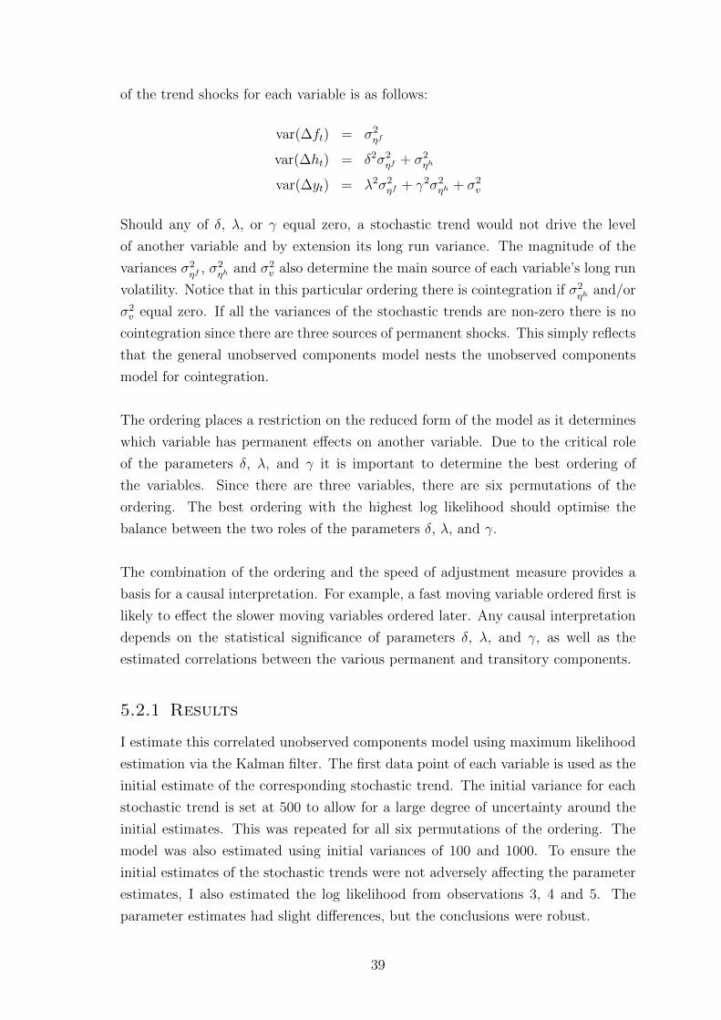
of the trend shocks for each variable is as follows:
var(∆ft) = σ2ηf
var(∆ht) = δ2σ2ηf + σ2
ηh
var(∆yt) = λ2σ2ηf + γ2σ2
ηh + σ2v
Should any of δ, λ, or γ equal zero, a stochastic trend would not drive the level
of another variable and by extension its long run variance. The magnitude of the
variances σ2ηf
, σ2ηh
and σ2v also determine the main source of each variable’s long run
volatility. Notice that in this particular ordering there is cointegration if σ2ηh
and/or
σ2v equal zero. If all the variances of the stochastic trends are non-zero there is no
cointegration since there are three sources of permanent shocks. This simply reflects
that the general unobserved components model nests the unobserved components
model for cointegration.
The ordering places a restriction on the reduced form of the model as it determines
which variable has permanent effects on another variable. Due to the critical role
of the parameters δ, λ, and γ it is important to determine the best ordering of
the variables. Since there are three variables, there are six permutations of the
ordering. The best ordering with the highest log likelihood should optimise the
balance between the two roles of the parameters δ, λ, and γ.
The combination of the ordering and the speed of adjustment measure provides a
basis for a causal interpretation. For example, a fast moving variable ordered first is
likely to effect the slower moving variables ordered later. Any causal interpretation
depends on the statistical significance of parameters δ, λ, and γ, as well as the
estimated correlations between the various permanent and transitory components.
5.2.1 Results
I estimate this correlated unobserved components model using maximum likelihood
estimation via the Kalman filter. The first data point of each variable is used as the
initial estimate of the corresponding stochastic trend. The initial variance for each
stochastic trend is set at 500 to allow for a large degree of uncertainty around the
initial estimates. This was repeated for all six permutations of the ordering. The
model was also estimated using initial variances of 100 and 1000. To ensure the
initial estimates of the stochastic trends were not adversely affecting the parameter
estimates, I also estimated the log likelihood from observations 3, 4 and 5. The
parameter estimates had slight differences, but the conclusions were robust.
39

The best ordering, with a log likelihood of -373.28 was real GDP, followed by
household credit and then firm credit:
yt = τ ft + uyt
ht = δτt + κht + uht
ft = λτt + γκht + κft + uyt
The parameter estimates from this ordering are presented in Table 5.3. The worst
ordering with the lowest log likelihood was firm credit, household credit then real
GDP. This preferred ordering based on the log likelihood of the model verifies earlier
evidence that the credit ratios do not drive permanent movements in real GDP.
The fastest moving variable as measured by the speed of adjustment is real GDP.
The impulse response functions of the transitory adjustments to a shock are shown
in Figure 5.2. Real GDP has a half-life of approximately two quarters, compared
to nearly 5 quarters for firm credit, and 10 quarters for household credit. Given
the model favoured ordering real GDP first, and the speed of adjustment shows real
GDP is the fastest moving variable, the unobserved component model, similarly to
the VECM, does not support that credit ratios have permanent effects on real GDP.
Strikingly, this model does not find evidence that real GDP has permanent effects
on the household credit and firm credit ratios either. The parameter estimates
of δ and λ are very low and the standard errors suggest these parameters are
statistically insignificant. Since these parameters are effectively zero, this indicates
a relationship with the level of credit. A permanent shock to real GDP increases the
denominator of the credit ratios. On average, the level of credit should also increase
by a proportionate amount so there in no permanent change in the credit ratios. The
parameter estimates of the variances are also well above zero, reinforcing the finding
of no cointegration. The lack of any substantive correlation between permanent
movements in real GDP and the credit ratios, as indicated by δ and λ, suggests
there is no long run relationship between financial deepening and output in the
United States.
While this unobserved components model does not find evidence that real GDP
has permanent effects on the credit ratios, the estimated correlations do show some
weak transitory effect. A natural interpretation of the correlation estimates is the
transitory adjustment towards a new long run level given a permanent shock. This
follows from invoking long run neutrality, the notion that demand side shocks do not
40
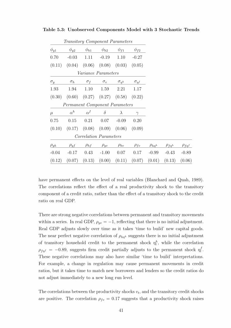
Table 5.3: Unobserved Components Model with 3 Stochastic Trends
Transitory Component Parameters
φy1 φy2 φh1 φh2 φf1 φf2
0.70 -0.03 1.11 -0.19 1.10 -0.27
(0.11) (0.04) (0.06) (0.08) (0.03) (0.05)
Variance Parameters
σy σh σf σv σηh σηf
1.93 1.94 1.10 1.59 2.21 1.17
(0.30) (0.60) (0.27) (0.27) (0.58) (0.22)
Permanent Component Parameters
µ αh αf δ λ γ
0.75 0.15 0.21 0.07 -0.09 0.20
(0.10) (0.17) (0.08) (0.09) (0.06) (0.09)
Correlation Parameters
ρyh ρyf ρhf ρyv ρhv ρfv ρhηh ρfηh ρfηf
-0.04 -0.17 0.43 -1.00 0.07 0.17 -0.99 -0.43 -0.89
(0.12) (0.07) (0.13) (0.00) (0.11) (0.07) (0.01) (0.13) (0.06)
have permanent effects on the level of real variables (Blanchard and Quah, 1989).
The correlations reflect the effect of a real productivity shock to the transitory
component of a credit ratio, rather than the effect of a transitory shock to the credit
ratio on real GDP.
There are strong negative correlations between permanent and transitory movements
within a series. In real GDP, ρyv = −1, reflecting that there is no initial adjustment.
Real GDP adjusts slowly over time as it takes ‘time to build’ new capital goods.
The near perfect negative correlation of ρhηh suggests there is no initial adjustment
of transitory household credit to the permanent shock ηht , while the correlation
ρfηf = −0.89, suggests firm credit partially adjusts to the permanent shock ηft .
These negative correlations may also have similar ‘time to build’ interpretations.
For example, a change in regulation may cause permanent movements in credit
ratios, but it takes time to match new borrowers and lenders so the credit ratios do
not adjust immediately to a new long run level.
The correlations between the productivity shocks vt, and the transitory credit shocks
are positive. The correlation ρfv = 0.17 suggests that a productivity shock raises
41

Figure 5.2: Impulse Response Functions for Transitory Componentswith 3 Stochastic Trends
0 5 10 15 20 25 30 35 40
quarters after shock
0
0.2
0.4
0.6
0.8
1
1.2
resp
onse
to s
hock
"half-life" line
real GDPhousehold creditfirm credit
expected aggregate income, which encourages borrowing, resulting in a positive
adjustment of firm credit to a new long run level. Since transitory real GDP does not
adjust immediately to the permanent productivity shock, while transitory firm credit
has a positive adjustment, the correlation between these two transitory components,
ρyf , is of the same magnitude but opposite sign to ρfv. The correlation ρhv shows a
very slight positive adjustment of transitory household credit to productivity shocks
vt.
There is some relationship between the two credit ratios. The parameter estimate of
γ is statistically significant, signifying that on average there is a positive correlation
between permanent movements in household and firm credit as credit markets
have deepened for both borrower groups. The correlation between the transitory
component of firm credit and permanent component of household credit ρfηh =
−0.43. This supports the initial finding that the two credit ratios have historically
offset each other, resulting in the aggregate credit ratio appearing stationary. Since
transitory household credit shows no initial adjustment to ηht , while transitory firm
credit has a negative adjustment, the correlation ρfh is of the same magnitude as
ρfηh but opposite sign.
42

5.3 Discussion of Findings
Using the unobserved components model has clarified earlier findings of the
cointegration analysis. I find real GDP, household credit and firm credit do not share
the same stochastic trend. When weakening this assumption so that permanent
shocks need not be perfectly correlated across variables, the model finds real GDP,
household credit and firm credit are driven by distinct stochastic trends. Since real
GDP has the fastest speed of adjustment, the VECM finding that real GDP is weakly
exogenous was not the result of low power to detect a slow moving endogenous
variable. Separating the aggregate credit ratio into household credit and firm credit
was useful for finding permanent movements, although this did not seem to matter in
terms of revealing differing effects. Neither credit ratio drives permanent movements
in real GDP and real GDP does not have permanent effects on the credit ratios, so
there is no long run relationship.
This conclusion may appear odd, particularly given the run-up in the credit ratios
prior to the Global Financial Crisis. It is important to draw a distinction between
the long run and short run. By long run, I mean that permanent movements in
the credit ratios do not drive permanent movements in real GDP, nor does real
GDP have permanent effects on the credit ratios. This is not to dismiss research
that shows short term credit booms increase the risk and severity of a financial crises
(Jorda et al., 2013). The parameter estimates reflect the average effect of permanent
shocks over 60 years of data. Generally, there has been an upward stochastic trend
in the credit ratios over the last 60 years. I find this financial deepening has not
been driving the mostly upward trend in output in the United States.
Closer inspection of the earlier cointegration analysis shows that allowing for three
stochastic trends is the better specification. Imposing cointegration resulted in
omitted stochastic trends and extremely persistent transitory components in the
VECM. Table 5.4 compares the sum of the auto-regressive parameters of the final
unobserved components model with ρ from the ADF test of the Engle-Granger
approach. Since the sum of the auto-regressive coefficients are noticeably lower, the
transitory components in the final unobserved components model are less persistent.
This reflects that the omitted stochastic trends were only fully accounted for once
allowing for three stochastic trends. This is also evident from the large variances of
the stochastic trends in Table 5.3, which also clearly indicate no cointegration.
This finding raises the question of why the Engle-Granger test appeared to offer
some evidence that the variables were cointegrated. The rejection of a true null
43

Table 5.4: Comparing the Persistence of Transitory Components
Dependent Variable
Log Real GDP Household Credit Firm Credit
φ1 + φ2 0.67 0.92 0.83
ρ 0.96 0.98 0.96
hypothesis may simply reflect that Type 1 errors occur when using the ADF test.
Overall, the results of the Engle-Granger and Johansen tests were mixed, neither
test conclusively indicated cointegration. The results of the Engle-Granger test
were reliant on the choice of dependent variable, since the residuals appeared
nonstationary when selecting household credit as the dependent variable. Using
insufficient lags for the Johansen test also created size distortions, leading to under-
rejection of stationarity in the error term. The Johansen test did reject cointegration
when properly specifying a sufficient number of lags to account for serial correlation.
While real GDP, household credit and firm credit have distinct stochastic trends, the
final unobserved components model indicates productivity shocks to real GDP may
have positive transitory effects on the credit ratios, particularly firm credit. These
correlations do not reflect permanent effects, but there is some dynamic response of
credit ratios to productivity shocks. Aside from the relationship between real GDP
and the credit ratios, the cointegration analysis, VECM and unobserved components
model suggest that on average the two credit ratios have historically been negatively
correlated.
These results are at odds with the broad conclusions of the financial development
literature and appear to more closely resemble the neoclassical view that finance is
not as fundamental to the real economy compared to other drivers of long run
growth. Although, there may be more nuanced reasons for not finding a long
run relationship. Empirical papers such as Rioja and Valev (2004) conclude the
relationship between private credit and real GDP is only weakly significant in
advanced economies, but stronger in middle-income economies. For a country like
the United States, the returns to greater levels of credit are insignificant once at the
technology frontier. For middle-income countries, the gains may be greater if higher
levels of credit can be used to make structural changes and achieve higher levels of
productivity (Aghion et al., 2005).
Failure to find a long run relationship between the credit ratios and real GDP
44

in either direction naturally raises a question as to what role omitted variables
may have played. The financial development literature has focussed on finding a
relationship between the private credit ratio and real GDP. The control variables
employed are other factors associated with economic growth such as the initial
level of output, average years of schooling, trade openness and legal origin of a
country (see Levine et al., 2000). Omitted variables such as interest rates or house
prices may be relevant for identifying short term, business cycle effects. If there
really is a long run relationship between real GDP and the credit ratios as well
as another variable, this variable would need to act in such a way to obscure the
missing long run relationship when omitted. When variables are cointegrated, but a
relevant first-order integrated variable omitted, the cointegration test result is often
spurious, indicating there is cointegration amongst included variables (Everaert,
2011). Using the unobserved components model to identify stochastic trends should
not be affected by omitted variables. The final unobserved components model
is designed to tease out correlations between permanent movements if they are
present in the data. Adding another variable to the unobserved component or the
cointegrating vector is feasible. Finding a relevant variable which stops real GDP
and the credit ratios arbitrarily moving away from their long run equilibrium is an
area of future research.
The lack of a long run relationship does not necessarily negate the importance
of finance since no attention was given to equity. Equity markets are very well
developed in the United States and make act as substitutes to credit markets.
Various papers (see Beck and Levine, 2004; Demirguc-Kunt, Feyen, and Levine,
2012) highlight the positive impact of stock market development indicators in panel
data studies of financial development and economic growth. In a time series analysis
of bank credit, stock market development and real GDP for 22 advanced economies,
Peia and Roszbach (2015) find stock market development usually causes growth,
but bank sector development usually follows real GDP. The causality tests for the
United States suggest real GDP causes bank credit, and there is a bi-directional
relationship between stock market development and real GDP. Using recent data,
Rousseau and Wachtel (2011) find the effect of finance diminishes even when allowing
for the combined effect of equity and credit together. The authors conclude that the
decline in the effect of financial deepening is the result of banking crises in recent
years.
45

5.3.1 Robustness to the Global Financial Crisis
To evaluate whether there was evidence of a long run relationship prior to the Global
Financial Crisis I re-estimate the final unobserved components model with a smaller
sample period that ends at 2008:Q1. The best ordering is still real GDP, household
credit and firm credit, with a log likelihood of -311.25. The parameter estimates are
presented in Table 5.5.
Table 5.5: Unobserved Components Model For 1952:Q1-2008:Q1
Transitory Component Parameters
φy1 φy2 φh1 φh2 φf1 φf2
0.41 0.10 1.18 -0.33 0.98 -0.16
(0.10) (0.09) (0.06) (0.08) (0.07) (0.07)
Variance Parameters
σy σh σf σv σηh σηf
1.48 0.83 1.13 1.58 1.21 1.23
(0.27) (0.24) (0.37) (0.30) (0.21) (0.30)
Permanent Component Parameters
µ αh αf δ λ γ
0.79 0.47 0.19 -0.17 -0.18 0.32
(0.10) (0.10) (0.12) (0.07) (0.10) (0.18)
Correlation Parameters
ρyh ρyf ρhf ρyv ρhv ρfv ρhηh ρfηh ρfηf
-0.37 -0.27 0.43 -1.00 0.32 0.26 -0.93 -0.36 -0.89
(0.09) (0.12) (0.13) (0.00) (0.10) (0.12) (0.04) (0.13) (0.06)
A clear difference is that the parameter estimates of δ and λ are statistically
significant and negative. This negative estimate suggests that prior to the Global
Financial Crisis, the model finds real GDP does not have permanent effects on the
level of credit. A positive permanent shock to real GDP increases the denominator
in the credit ratios. All else being equal, if the level of credit does not respond, there
is a negative relationship between real GDP and the credit ratios.
Over the full sample, the average effect of real GDP on the level of credit is one-for-
one, as there are no permanent effects of real GDP on the credit ratios. Including
the data after 2008 indicates that the Global Financial Crisis did affect credit levels
46

so that the credit ratios declined while the denominator decreased. As seen in
Figure 3.2, the decline in real GDP and the credit ratios was synchronised during
the Global Financial Crisis, whereas during previous recession periods the credit
ratios often increase. This effect during the Global Financial Crisis changed the
parameters estimates of δ and λ from negative to zero. Using the full sample shows
that in the long run, real GDP can have permanent effects on the credit levels.
It is widely accepted that the credit boom during the 2000s played a key role in the
severity of the Global Financial Crisis. The estimates presented here reflect that
on average, credit ratios do not predict the level of output. On average, increases
in the credit ratios are not due to credit booms, but further financial deepening.
In other orderings using this smaller sample, the δ and λ parameters which reflect
the effect of credit ratios on permanent movements in real GDP are not statistically
significant. Figure 5.3 shows that the credit ratios adjust more slowly than real
GDP, so it is real GDP that Granger causes the credit ratios on average.
Figure 5.3: Impulse Response Functions for Transitory Components of1952:Q1-2008:Q1 Sample
0 5 10 15 20 25 30 35 40
quarters after shock
0
0.2
0.4
0.6
0.8
1
1.2
resp
onse
to s
hock
"half-life" line
real GDPhousehold creditfirm credit
Other notable differences in the parameter estimates are the variance parameters
and correlations. The variance of transitory and permanent household credit are
markedly lower as the large shock in 2008 is not included in the sample. The
47

correlation with transitory household credit and permanent real GDP, ρhv = 0.32,
and the correlation with transitory firm credit and permanent real GDP, ρfv = 0.26.
Permanent productivity shocks did not have as strong a positive effect when using
the full sample. This may reflect that after the Global Financial Crisis, credit ratios
stayed depressed while output recovered.
48
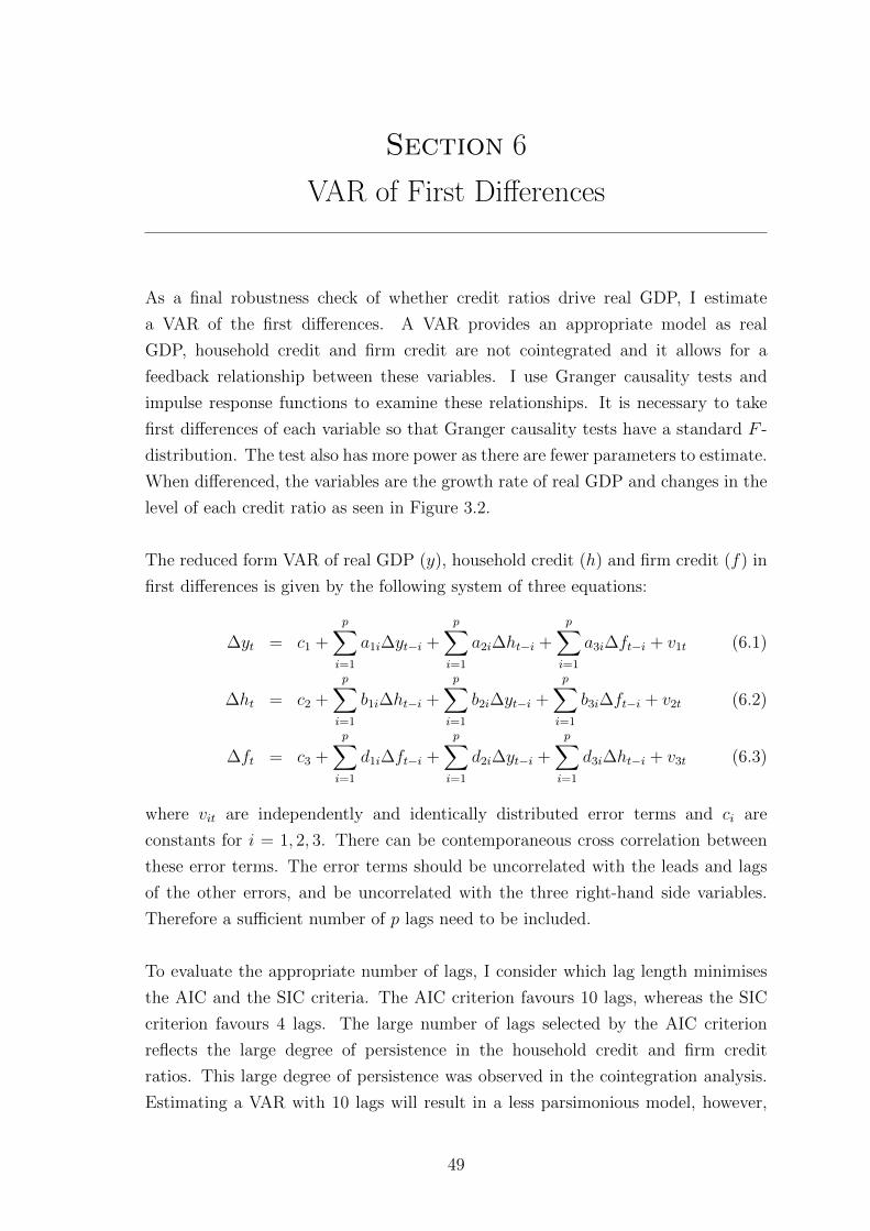
Section 6
VAR of First Differences
As a final robustness check of whether credit ratios drive real GDP, I estimate
a VAR of the first differences. A VAR provides an appropriate model as real
GDP, household credit and firm credit are not cointegrated and it allows for a
feedback relationship between these variables. I use Granger causality tests and
impulse response functions to examine these relationships. It is necessary to take
first differences of each variable so that Granger causality tests have a standard F -
distribution. The test also has more power as there are fewer parameters to estimate.
When differenced, the variables are the growth rate of real GDP and changes in the
level of each credit ratio as seen in Figure 3.2.
The reduced form VAR of real GDP (y), household credit (h) and firm credit (f) in
first differences is given by the following system of three equations:
∆yt = c1 +
p∑i=1
a1i∆yt−i +
p∑i=1
a2i∆ht−i +
p∑i=1
a3i∆ft−i + v1t (6.1)
∆ht = c2 +
p∑i=1
b1i∆ht−i +
p∑i=1
b2i∆yt−i +
p∑i=1
b3i∆ft−i + v2t (6.2)
∆ft = c3 +
p∑i=1
d1i∆ft−i +
p∑i=1
d2i∆yt−i +
p∑i=1
d3i∆ht−i + v3t (6.3)
where vit are independently and identically distributed error terms and ci are
constants for i = 1, 2, 3. There can be contemporaneous cross correlation between
these error terms. The error terms should be uncorrelated with the leads and lags
of the other errors, and be uncorrelated with the three right-hand side variables.
Therefore a sufficient number of p lags need to be included.
To evaluate the appropriate number of lags, I consider which lag length minimises
the AIC and the SIC criteria. The AIC criterion favours 10 lags, whereas the SIC
criterion favours 4 lags. The large number of lags selected by the AIC criterion
reflects the large degree of persistence in the household credit and firm credit
ratios. This large degree of persistence was observed in the cointegration analysis.
Estimating a VAR with 10 lags will result in a less parsimonious model, however,
49

due to the importance of removing the serial correlation in the error terms I estimate
the model using 10 lags instead of 4. The estimates of the VAR in first differences
are presented in Table B.1.
6.1 Granger Causality Tests
I conduct Granger causality tests to evaluate whether changes in household credit
and firm credit effect real GDP growth. A variable is said to Granger-cause
another variable if its past values contain information that can help forecast the
contemporaneous values of the other variable. This is not equivalent to testing
if a variable is exogenous since it does not consider the contemporaneous effects of
variables on each other. Granger causality does indicate there is correlation between
variables and indicates the direction of the relationship.
Each equation of the VAR is estimated separately by OLS. The coefficients of one
lagged independent variable are jointly restricted to zero. If the null hypothesis of
the F-test is rejected, the coefficients are not jointly zero which indicates there is
Granger causality. Since there are three equations with two explanatory variables
each, there are six Granger causality tests. The results of the Granger causality
tests are presented in Table 6.1.
The Granger causality tests indicate that at the 5% significance level there are two
instances of Granger causality: real GDP growth Granger-causes ∆ft, and ∆ht
Granger-causes ∆ft. It is narrowly rejected that real GDP growth Granger-causes
∆ht. These Granger causality results reaffirm the previous findings of earlier models
that neither household credit nor firm credit have permanent effects on real GDP.
These results also align with the best ordering of the final unobserved components
model. At a 10% significance level, I find ∆ht Grange-causes real GDP growth.
Overall, it appears that lags of real GDP can help to forecast contemporaneous
values of the credit variables. ∆ht may have some predictive ability as well. These
Granger causality tests likely reflect there are statistically significant short term
effects rather than long run effects.
6.2 Impulse Responses: Short and Long Run Restrictions
The impulse response functions show the dynamic response of real GDP, household
credit and firm credit to a structural shock in each variable. While the unobserved
components model decomposes a series into permanent and transitory shocks, the
VAR structural shocks are not necessarily permanent shocks. The structural shocks
50

Table 6.1: Granger Causality Tests
Dependent Variable Independent Variable F-statistic p-value
∆Log Real GDP ∆Household Credit 1.64 0.10
∆Log Real GDP ∆Firm Credit 0.96 0.48
∆Household Credit ∆Log Real GDP 1.84 0.06
∆Household Credit ∆Firm Credit 1.47 0.15
∆Firm Credit ∆Log Real GDP 4.68 0
∆Firm Credit ∆Household Credit 3.16 0
are sensitive to the choice of identification strategy. I use the VAR impulse response
functions as a robustness check on the unobserved components model results.
I first use the Choleski decomposition to identify the structural model of the VAR
(see Appendix B.2). The variables are ordered real GDP growth, followed by ∆ht
and then ∆ft. This allows real GDP growth to have contemporaneous effects on
the two credit ratios. Household credit may have contemporaneous effects on firm
credit but not real GDP. This short run restriction is informed by the results of the
Granger causality tests and the earlier results of the unobserved components model.
Figure 6.1 shows the accumulated impulse response functions to a one standard
deviation exogenous structural shock, with two times the standard error bands.
By accumulating the response, the impulse response function reflects the effect on
the variable in levels and is directly comparable to the VECM impulse response
functions presented in Figure 4.2. There are some similarities between the impulse
response functions in Figure 4.2 and Figure 6.1. As seen along the main diagonal, the
effect of a structural shock to a variable has permanent effects on that same variable.
Most other impulse responses do not appear to be statistically different from zero at
long horizons. While the point estimates may indicate long run relationships exist,
the standard error bands suggest these are not statistically significant from zero.
This is in line with the unobserved components model finding that there is no long
run relationship between the real GDP and the credit ratios.
There does appear to be statistically significant transitory effects. The accumulated
response of ∆ft to a structural shock to real GDP growth is statistically significant
around 10 quarters. This supports the positive correlation of ρfv found in the
final unobserved components model. At the 10 quarter mark, given a one standard
51
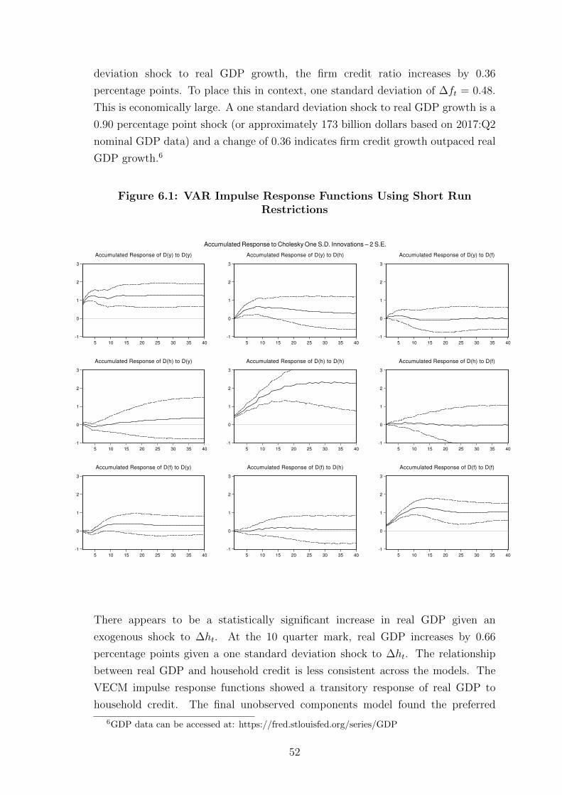
deviation shock to real GDP growth, the firm credit ratio increases by 0.36
percentage points. To place this in context, one standard deviation of ∆ft = 0.48.
This is economically large. A one standard deviation shock to real GDP growth is a
0.90 percentage point shock (or approximately 173 billion dollars based on 2017:Q2
nominal GDP data) and a change of 0.36 indicates firm credit growth outpaced real
GDP growth.6
Figure 6.1: VAR Impulse Response Functions Using Short RunRestrictions
-1
0
1
2
3
5 10 15 20 25 30 35 40
Accumulated Response of D(y) to D(y)
-1
0
1
2
3
5 10 15 20 25 30 35 40
Accumulated Response of D(y) to D(h)
-1
0
1
2
3
5 10 15 20 25 30 35 40
Accumulated Response of D(y) to D(f)
-1
0
1
2
3
5 10 15 20 25 30 35 40
Accumulated Response of D(h) to D(y)
-1
0
1
2
3
5 10 15 20 25 30 35 40
Accumulated Response of D(h) to D(h)
-1
0
1
2
3
5 10 15 20 25 30 35 40
Accumulated Response of D(h) to D(f)
-1
0
1
2
3
5 10 15 20 25 30 35 40
Accumulated Response of D(f) to D(y)
-1
0
1
2
3
5 10 15 20 25 30 35 40
Accumulated Response of D(f) to D(h)
-1
0
1
2
3
5 10 15 20 25 30 35 40
Accumulated Response of D(f) to D(f)
Accumulated Response to Cholesky One S.D. Innovations – 2 S.E.
There appears to be a statistically significant increase in real GDP given an
exogenous shock to ∆ht. At the 10 quarter mark, real GDP increases by 0.66
percentage points given a one standard deviation shock to ∆ht. The relationship
between real GDP and household credit is less consistent across the models. The
VECM impulse response functions showed a transitory response of real GDP to
household credit. The final unobserved components model found the preferred
6GDP data can be accessed at: https://fred.stlouisfed.org/series/GDP
52

ordering was to let real GDP drive household credit. This chosen ordering did
not allow the stochastic trend in household credit to be correlated with transitory
real GDP.
Using a Choleski decomposition does not allow both real GDP growth and ∆ht to
have contemporaneous effects on each other. The impulse response functions do not
change significantly with the ordering of the short run restrictions. To examine the
implications of using short run restrictions I also estimate a structural VAR using
long run restrictions as proposed by Blanchard and Quah (1989) (see Appendix B.2).
I assume that neither ∆ht nor ∆ft have long run effects on real GDP growth. This
forces the accumulated response function to tend to zero but allows the credit ratios
to have contemporaneous effects on real GDP growth. A third long run restriction
is necessary to identify the model. Given the Granger causality tests, I also assume
that ∆ft has no long run effect on ∆ht.7
Figure 6.2 displays the impulse response functions using long run restrictions.8 The
impulse response functions are effectively the same with the exception that the
effect of ∆ht on real GDP growth is clearly transitory and the response of ∆ht to
a structural shock to real GDP growth is larger. The point estimates suggest this
is a permanent response, although without the standard error bands it may not be
statistically significant at the longer horizons.
These impulse response functions show that the results are sensitive to the choice
of identification strategy. Allowing ∆ht to have contemporaneous effects on real
GDP growth but not a long run effect may be more appropriate. The VECM,
unobserved components model and Granger causality tests did not convincingly
show household credit has permanent effects on real GDP, but do suggest there
could be some transitory effect. A recent paper by Mian, Sufi, and Verner (2017)
finds the household credit to GDP ratio is contemporaneously associated with an
increase in consumption, but predicts lower GDP growth in the medium term.
Overall, the VAR shows the unobserved components model results are robust.
Movements in the credit ratios do not have statistically significant permanent effects
on real GDP. Real GDP does have some positive transitory effect on the credit ratios.
This may reflect that as productivity shocks to real GDP increase expected aggregate
income, households and firms are encouraged to borrow temporarily.
7Ideally one could have a mixture of long run and short run restrictions so that the other twolong run restrictions were not necessary. This is not possible in EViews.
8EViews does not generate standard error bands when using long run restrictions.
53

Figure 6.2: VAR Impulse Response Functions Using Long RunRestrictions
-0.5
0.0
0.5
1.0
1.5
2.0
2.5
5 10 15 20 25 30 35 40
Accumulated Response of D(y) to Shock1
-0.5
0.0
0.5
1.0
1.5
2.0
2.5
5 10 15 20 25 30 35 40
Accumulated Response of D(y) to Shock2
-0.5
0.0
0.5
1.0
1.5
2.0
2.5
5 10 15 20 25 30 35 40
Accumulated Response of D(y) to Shock3
-0.5
0.0
0.5
1.0
1.5
2.0
2.5
5 10 15 20 25 30 35 40
Accumulated Response of D(h) to Shock1
-0.5
0.0
0.5
1.0
1.5
2.0
2.5
5 10 15 20 25 30 35 40
Accumulated Response of D(h) to Shock2
-0.5
0.0
0.5
1.0
1.5
2.0
2.5
5 10 15 20 25 30 35 40
Accumulated Response of D(h) to Shock3
-0.5
0.0
0.5
1.0
1.5
2.0
2.5
5 10 15 20 25 30 35 40
Accumulated Response of D(f) to Shock1
-0.5
0.0
0.5
1.0
1.5
2.0
2.5
5 10 15 20 25 30 35 40
Accumulated Response of D(f) to Shock2
-0.5
0.0
0.5
1.0
1.5
2.0
2.5
5 10 15 20 25 30 35 40
Accumulated Response of D(f) to Shock3
Accumulated Response to Structural One S.D. Innovations
54
Section 7
Conclusion
The common finding of the financial development literature, that finance causes
growth, is not evident in this data for the United States. Disaggregating private
credit into household and firm credit gives clearer evidence of permanent movements
compared to the aggregate measure of credit. While this creates the possibility of
a cointegrating relationship, I do not find one exists. Using disaggregated credit
data also allows for differing effects between household credit and firm credit. Given
recent empirical research such as Beck et al. (2012), one may have anticipated that
the ratio of firm credit would have a positive long run relationship with real GDP,
but this is not evident in the US data. Using a variety of time series models, I
find robust evidence that permanent movements in the credit ratios do not cause
permanent movements in real GDP.
The unobserved components model presented in this thesis has the advantage of
identifying permanent shocks and evaluating whether permanent movements are
common across variables. To the best of my knowledge, unobserved components
models have not been used in the finance-growth literature before. Using this model
clarified that imposing cointegration on these variables omits stochastic trends.
Allowing for three stochastic trends in a way that lets permanent movements in
real GDP drive the credit ratios is the best specification. The speed of adjustment
measure provided by the unobserved components model reinforces this is the
best specification, and the correlation estimates suggest permanent movements in
real GDP have a positive transitory effect on the credit ratios. The key focus
though is the long run relationship, and the unobserved components model finds no
substantive correlation between the permanent movements. This suggests that on
average, there is a one-for-one relationship between permanent movements in real
GDP and the level of credit, which results in no change in the credit ratios.
These findings support recent empirical research by Arcand et al. (2015) and
Rousseau and Wachtel (2011), that the upside benefit of financial deepening derived
from cross-country studies of the 1990s is simplistic, particularly in consideration
of the potentially severe downside financial risks at higher credit ratios. This is
especially true in advanced economies where credit ratios tend to be highest. This
55
finding supports the notion that the returns to higher levels of financial deepening
are not significant at the technology frontier. Credit ratios, as a proxy for financial
deepening or otherwise, do not appear to be a key determinant of long run economic
output, at least in the United States.
Since real GDP is not found to have permanent effects on the credit ratios either,
a natural question to ask is “what does?”. Real GDP may have transitory effects
on the credit ratios but cannot explain the permanent movements. Changes in
regulations are likely to be a critical determinant. Quantifying these factors is
difficult in a time series context, but may explain permanent movements observed
in these credit ratios.
Whether other variables should be included to find a cointegrating relationship is an
open question. If there are relevant first-order integrated variables that have been
omitted, another unobserved components model approach proposed by Everaert
(2011) is to model the error term as a random walk and transitory component. If
the model is specified correctly, this can be shown to capture the omitted variable
and estimate the long run relationship between the observed variables.
The unobserved components model presented here can be applied to other types
of data and other countries for future research. A key question is whether these
findings are consistent with other advanced economies at the technology frontier.
Since countries have differently structured financial systems there may be a large
degree of heterogeneity even within countries of the same broad income group. The
ratios of household credit and firm credit could be replaced by other finance measures
such as the ratio of domestic bank credit to GDP and stock market capitalisation
to evaluate the long run role of different types of finance. While the financial
development literature has focussed on real GDP, there may be clearer signals of
long run relationship when focussing on specific channels such as physical capital
accumulation or productivity instead. These various extensions may highlight
nuances in the finance-growth relationship that is increasingly the focus empirical
research.
56

Appendix A
Cointegration Analysis and VECM
A.1 Unit Root Tests
Table A.1: ADF-GLS Tests for Unit Roots
Variable Lags t-statistic critical value a
Household Credit 14 -2.79 -2.92
Firm Credit 10 -2.31 -2.92
Total Credit 9 -3.43 -2.92
Real GDP 1 -0.72 -2.91a Elliott et al. (1996) critical values
Table A.2: KPSS Tests for Unit Roots
Variable t-statistic critical valuea
Household Credit 0.23 0.15
Firm Credit 0.25 0.15
Total Credit 0.09 0.15
Real GDP 0.37 0.15a Kwiatkowski et al. (1992) critical values
Table A.3: ADF Tests for Unit Roots of First Differences
Variable Lags t-statistic p-valuea
∆ Household Credit 13 -3.24 0.02
∆ Firm Credit 9 -4.86 0
∆ Total Credit 13 -4.11 0
∆ Real GDP 0 -11.26 0a MacKinnon (1996) one-sided p-values
57
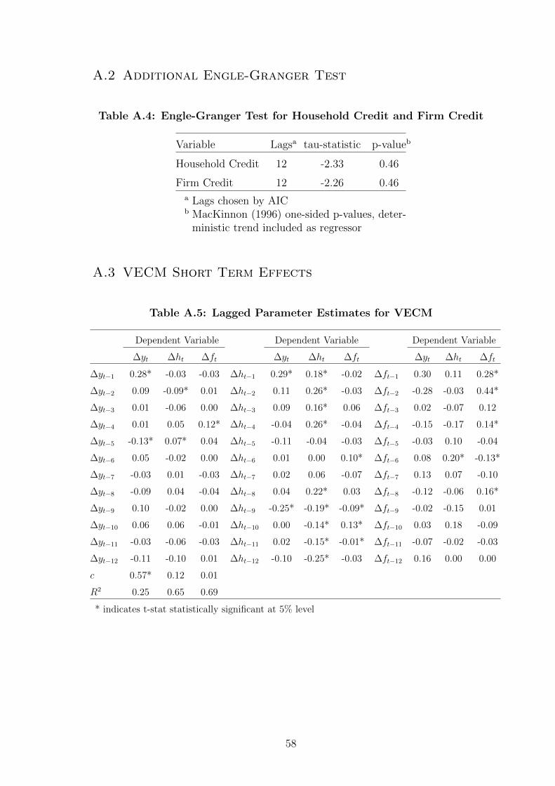
A.2 Additional Engle-Granger Test
Table A.4: Engle-Granger Test for Household Credit and Firm Credit
Variable Lagsa tau-statistic p-valueb
Household Credit 12 -2.33 0.46
Firm Credit 12 -2.26 0.46a Lags chosen by AICb MacKinnon (1996) one-sided p-values, deter-
ministic trend included as regressor
A.3 VECM Short Term Effects
Table A.5: Lagged Parameter Estimates for VECM
Dependent Variable Dependent Variable Dependent Variable
∆yt ∆ht ∆ft ∆yt ∆ht ∆ft ∆yt ∆ht ∆ft
∆yt−1 0.28* -0.03 -0.03 ∆ht−1 0.29* 0.18* -0.02 ∆ft−1 0.30 0.11 0.28*
∆yt−2 0.09 -0.09* 0.01 ∆ht−2 0.11 0.26* -0.03 ∆ft−2 -0.28 -0.03 0.44*
∆yt−3 0.01 -0.06 0.00 ∆ht−3 0.09 0.16* 0.06 ∆ft−3 0.02 -0.07 0.12
∆yt−4 0.01 0.05 0.12* ∆ht−4 -0.04 0.26* -0.04 ∆ft−4 -0.15 -0.17 0.14*
∆yt−5 -0.13* 0.07* 0.04 ∆ht−5 -0.11 -0.04 -0.03 ∆ft−5 -0.03 0.10 -0.04
∆yt−6 0.05 -0.02 0.00 ∆ht−6 0.01 0.00 0.10* ∆ft−6 0.08 0.20* -0.13*
∆yt−7 -0.03 0.01 -0.03 ∆ht−7 0.02 0.06 -0.07 ∆ft−7 0.13 0.07 -0.10
∆yt−8 -0.09 0.04 -0.04 ∆ht−8 0.04 0.22* 0.03 ∆ft−8 -0.12 -0.06 0.16*
∆yt−9 0.10 -0.02 0.00 ∆ht−9 -0.25* -0.19* -0.09* ∆ft−9 -0.02 -0.15 0.01
∆yt−10 0.06 0.06 -0.01 ∆ht−10 0.00 -0.14* 0.13* ∆ft−10 0.03 0.18 -0.09
∆yt−11 -0.03 -0.06 -0.03 ∆ht−11 0.02 -0.15* -0.01* ∆ft−11 -0.07 -0.02 -0.03
∆yt−12 -0.11 -0.10 0.01 ∆ht−12 -0.10 -0.25* -0.03 ∆ft−12 0.16 0.00 0.00
c 0.57* 0.12 0.01
R2 0.25 0.65 0.69
* indicates t-stat statistically significant at 5% level
58

Appendix B
VAR
B.1 VAR Estimates
Table B.1: Parameter Estimates for VAR in First Differences
Dependent Variable Dependent Variable Dependent Variable
∆yt ∆ht ∆ft ∆yt ∆ht ∆ft ∆yt ∆ht ∆ft
∆yt−1 0.29* -0.02 -0.03 ∆ht−1 0.32* 0.19* -0.01 ∆ft−1 0.37* 0.13 0.28*
∆yt−2 0.08 -0.07* 0.01 ∆ht−2 0.12 0.26* -0.01 ∆ft−2 -0.30 0.08 0.44*
∆yt−3 0.01 -0.70* 0.01 ∆ht−3 0.09 0.11* 0.06 ∆ft−3 0.05 -0.15 0.12
∆yt−4 0.02 0.07* 0.13* ∆ht−4 -0.09 0.33* -0.05 ∆ft−4 -0.10 -0.15 0.14*
∆yt−5 -0.16* 0.07* 0.04 ∆ht−5 -0.12 -0.06 -0.03 ∆ft−5 -0.05 0.02 -0.04
∆yt−6 0.03 -0.02 0.01 ∆ht−6 0.02 0.00 0.09* ∆ft−6 0.01 0.21* -0.15*
∆yt−7 -0.02 0.03 -0.03 ∆ht−7 0.00 -0.02 -0.09* ∆ft−7 0.01 -0.06 -0.12*
∆yt−8 -0.08 0.03 -0.03 ∆ht−8 -0.01 0.27* 0.02 ∆ft−8 -0.17 -0.16 0.17*
∆yt−9 0.12 -0.02 0.00 ∆ht−9 -0.27* -0.18* -0.01* ∆ft−9 0.05 -0.10 -0.01
∆yt−10 0.02 0.04 -0.02 ∆ht−10 0.25 -0.13* 0.11* ∆ft−10 0.18 0.19* -0.11*
c 0.50* 0.02 -0.02
R2 0.25 0.60 0.68
* indicates t-stat statistically significant at 5% level
59

B.2 Structural Identification
A Structural VAR (SVAR) represents the contemporaneous and lagged effects of a
system of n endogenous variables. The (n×1) matrix Yt has SVAR(p) representation:
Θ−10 Yt = Γ(L)Yt + εt, εt ∼ i.i.d.(0, I)
The reduced-form VAR(p) representation is given by:
Yt = Θ0Γ(L)LYt + Θ0εt
= Φ + Φ(L)LYt + et, et ∼ i.i.d.(0,Ω)
Short run restrictions: Choleski Decomposition
Θ0εt = et. Since et are observed, to identify the structural innovations (εt)n2−n
2
restrictions are imposed on Θ−10 . Using short run restrictions assumes Θ0 is a
lower-triangular matrix, so a variable has contemporaneous effects only on variables
ordered after it. Notice that Ω = Θ0Θ′0. Using the Choleski decomposition, the
variance-covariance matrix Ω is decomposed into a lower-triangular matrix and its
transpose. Therefore Θ0 = chol(Ω), where Θ0 is a lower triangular matrix.
Long run restrictions
The reduced-form VAR can be rewritten as:
[I − Θ0Γ(L)L]Yt = Θ0εt
Yt = [I − Θ0Γ(L)L]−1Θ0εt
C = [I − Θ0Γ(L)L]−1Θ0 reflects the cumulative effect of the structural shocks on
Yt. Assuming that a structural shock εj has no long run effect on variable yi implies
Cij = 0. Imposing n2−n2
restrictions on matrix C can be shown to recover the
structural shocks (see Enders, 2008, p. 215).
60
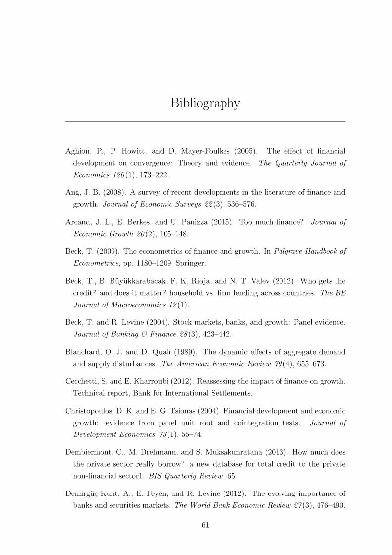
Bibliography
Aghion, P., P. Howitt, and D. Mayer-Foulkes (2005). The effect of financial
development on convergence: Theory and evidence. The Quarterly Journal of
Economics 120 (1), 173–222.
Ang, J. B. (2008). A survey of recent developments in the literature of finance and
growth. Journal of Economic Surveys 22 (3), 536–576.
Arcand, J. L., E. Berkes, and U. Panizza (2015). Too much finance? Journal of
Economic Growth 20 (2), 105–148.
Beck, T. (2009). The econometrics of finance and growth. In Palgrave Handbook of
Econometrics, pp. 1180–1209. Springer.
Beck, T., B. Buyukkarabacak, F. K. Rioja, and N. T. Valev (2012). Who gets the
credit? and does it matter? household vs. firm lending across countries. The BE
Journal of Macroeconomics 12 (1).
Beck, T. and R. Levine (2004). Stock markets, banks, and growth: Panel evidence.
Journal of Banking & Finance 28 (3), 423–442.
Blanchard, O. J. and D. Quah (1989). The dynamic effects of aggregate demand
and supply disturbances. The American Economic Review 79 (4), 655–673.
Cecchetti, S. and E. Kharroubi (2012). Reassessing the impact of finance on growth.
Technical report, Bank for International Settlements.
Christopoulos, D. K. and E. G. Tsionas (2004). Financial development and economic
growth: evidence from panel unit root and cointegration tests. Journal of
Development Economics 73 (1), 55–74.
Dembiermont, C., M. Drehmann, and S. Muksakunratana (2013). How much does
the private sector really borrow? a new database for total credit to the private
non-financial sector1. BIS Quarterly Review , 65.
Demirguc-Kunt, A., E. Feyen, and R. Levine (2012). The evolving importance of
banks and securities markets. The World Bank Economic Review 27 (3), 476–490.
61

Elliott, G., T. J. Rothenberg, and J. H. Stock (1996). Efficient tests for an
autoregressive unit root. Econometrica 64 (4), 813–836.
Enders, W. (2008). Applied Econometric Time Series. John Wiley & Sons.
Everaert, G. (2011). Estimation and inference in time series with omitted i (1)
variables. Journal of Time Series Econometrics 2 (2), 1–28.
Fink, G., P. R. Haiss, and S. Hristoforova (2003). Bond markets and economic
growth.
Gonzalo, J. and S. Ng (2001). A systematic framework for analyzing the dynamic
effects of permanent and transitory shocks. Journal of Economic Dynamics and
Control 25 (10), 1527–1546.
Greenwood, J. and B. Jovanovic (1990). Financial development, growth, and the
distribution of income. Journal of Political Economy 98 (5, Part 1), 1076–1107.
Greenwood, R. and D. Scharfstein (2013). The growth of finance. The Journal of
Economic Perspectives 27 (2), 3–28.
Harvey, A. C. (1985). Trends and cycles in macroeconomic time series. Journal of
Business & Economic Statistics 3 (3), 216–227.
Harvey, A. C. (1993). Time series models, Volume 2. Harvester Wheatsheaf New
York.
Hung, F.-S. (2009). Explaining the nonlinear effects of financial development on
economic growth. Journal of Economics 97 (1), 41–65.
Jayaratne, J. and P. E. Strahan (1996). The finance-growth nexus: Evidence from
bank branch deregulation. The Quarterly Journal of Economics 111 (3), 639–670.
Jorda, O., M. Schularick, and A. M. Taylor (2013). When credit bites back. Journal
of Money, Credit and Banking 45 (s2), 3–28.
Kim, C.-J. and C. R. Nelson (1999). State-space models with regime switching:
classical and gibbs-sampling approaches with applications. MIT Press Books 1.
King, R. G. and R. Levine (1993). Finance and growth: Schumpeter might be right.
The Quarterly Journal of Economics 108 (3), 717–737.
Kwiatkowski, D., P. C. Phillips, P. Schmidt, and Y. Shin (1992). Testing the null
hypothesis of stationarity against the alternative of a unit root: How sure are we
that economic time series have a unit root? Journal of Econometrics 54 (1-3),
159–178.
62

Kydland, F. E. and E. C. Prescott (1982). Time to build and aggregate fluctuations.
Econometrica 50 (6), 1345–1370.
Law, S. H. and N. Singh (2014). Does too much finance harm economic growth?
Journal of Banking & Finance 41, 36–44.
Lettau, M. and S. C. Ludvigson (2014). Shocks and crashes. NBER Macroeconomics
Annual 28 (1), 293–354.
Levine, R. (2005). Finance and growth: theory and evidence. Handbook of economic
growth 1, 865–934.
Levine, R., N. Loayza, and T. Beck (2000). Financial intermediation and growth:
Causality and causes. Journal of monetary Economics 46 (1), 31–77.
Loayza, N. V. and R. Ranciere (2006). Financial development, financial fragility,
and growth. Journal of Money, Credit and Banking 38 (4), 1051–1076.
Luintel, K. B. and M. Khan (1999). A quantitative reassessment of the finance–
growth nexus: evidence from a multivariate var. Journal of Development
Economics 60 (2), 381–405.
Luintel, K. B., M. Khan, P. Arestis, and K. Theodoridis (2008). Financial structure
and economic growth. Journal of Development Economics 86 (1), 181–200.
MacKinnon, J. G. (1996). Numerical distribution functions for unit root and
cointegration tests. Journal of Applied Econometrics 11 (6), 601–618.
MacKinnon, J. G., A. A. Haug, and L. Michelis (1999). Numerical distribution
functions of likelihood ratio tests for cointegration. Journal of applied
Econometrics 14 (5), 563–577.
McKinnon, R. (1973). Money and capital. Economic Development .
Mian, A., A. Sufi, and E. Verner (2017). Household debt and business cycles
worldwide. The Quarterly Journal of Economics 132 (4), 17551817.
Morley, J. C. (2007). The slow adjustment of aggregate consumption to permanent
income. Journal of Money, Credit and Banking 39 (2-3), 615–638.
Morley, J. C., C. R. Nelson, and E. Zivot (2003). Why are the beveridge-nelson
and unobserved-components decompositions of gdp so different? The Review of
Economics and Statistics 85 (2), 235–243.
63

Ng, S. and P. Perron (1995). Unit root tests in arma models with data-dependent
methods for the selection of the truncation lag. Journal of the American Statistical
Association 90 (429), 268–281.
Pagan, A. R. and M. H. Pesaran (2008). Econometric analysis of structural systems
with permanent and transitory shocks. Journal of Economic Dynamics and
Control 32 (10), 3376–3395.
Pagano, M. (1993). Financial markets and growth: an overview. European economic
review 37 (2-3), 613–622.
Peia, O. and K. Roszbach (2015). Finance and growth: time series evidence on
causality. Journal of Financial Stability 19, 105–118.
Philippon, T. and A. Reshef (2013). An international look at the growth of modern
finance. The Journal of Economic Perspectives 27 (2), 73–96.
Rajan, R. G. and L. Zingales (1998). Financial dependence and growth. The
American Economic Review 88 (3), 559–586.
Rioja, F. and N. Valev (2004). Does one size fit all?: a reexamination of the finance
and growth relationship. Journal of Development economics 74 (2), 429–447.
Rousseau, P. L. and P. Wachtel (2011). What is happening to the impact of financial
deepening on economic growth? Economic Inquiry 49 (1), 276–288.
Sassi, S. and A. Gasmi (2014). The effect of enterprise and household credit on
economic growth: New evidence from european union countries. Journal of
Macroeconomics 39, 226–231.
Schleicher, C. (2003). Structural time series models with common trends and
common cycles. University of British Columbia.
Shaw, E. S. (1973). Financial deepening in economic development.
Sinclair, T. M. (2009). The relationships between permanent and transitory
movements in us output and the unemployment rate. Journal of Money, Credit
and Banking 41 (2-3), 529–542.
Stock, J. H. and M. W. Watson (1988). Testing for common trends. Journal of the
American Statistical Association 83 (404), 1097–1107.
Stock, J. H. and M. W. Watson (1993). A simple estimator of cointegrating vectors
in higher order integrated systems. Econometrica 61 (4), 783–820.
Trenkler, C. and E. Weber (2016). On the identification of multivariate correlated
unobserved components models. Economics Letters 138, 15–18.
64
Top Related