Space Sci Rev (2010) 152: 591–616DOI 10.1007/s11214-009-9579-5

The Solar Dynamo

Chris A. Jones · Michael J. Thompson ·Steven M. Tobias

Received: 24 June 2009 / Accepted: 12 October 2009 / Published online: 19 December 2009© Springer Science+Business Media B.V. 2009

Abstract Observations relevant to current models of the solar dynamo are presented, withemphasis on the history of solar magnetic activity and on the location and nature of the solartachocline. The problems encountered when direct numerical simulation is used to analysethe solar cycle are discussed, and recent progress is reviewed. Mean field dynamo theory isstill the basis of most theories of the solar dynamo, so a discussion of its fundamental prin-ciples and its underlying assumptions is given. The role of magnetic helicity is discussed.Some of the most popular models based on mean field theory are reviewed briefly. Dynamomodels based on severe truncations of the full MHD equations are discussed.

Keywords Solar magnetism · Solar dynamo · Sunspots · Solar cycles · Solar interior ·Helioseismology

1 Observations

1.1 Sunspots and Solar Magnetic Activity

Sunspots are perhaps the most obvious manifestation of solar magnetism (Thomas and Weiss2008). Sunspots were observed already by the ancients, and were shown by Galileo to befeatures on the Sun itself; but the observational evidence that sunspots possess magneticfields was established only a hundred years ago by Hale (1908). The number of sunspots,or the area occupied by them, follows an irregular 11-year activity cycle (lower panel of

C.A. Jones (�) · S.M. TobiasDepartment of Applied Mathematics, University of Leeds, Leeds LS2 9JT, UKe-mail: cajones@maths.leeds.ac.uk

S.M. Tobiase-mail: smt@maths.leeds.ac.uk

M.J. ThompsonSchool of Mathematics and Statistics, University of Sheffield, Sheffield S3 7RH, UKe-mail: michael.thompson@sheffield.ac.uk

592 C.A. Jones et al.

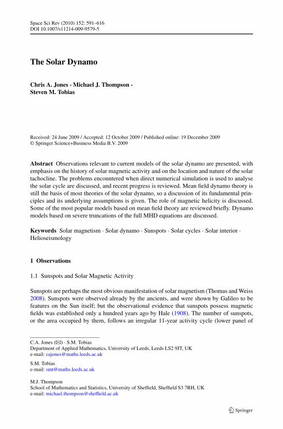
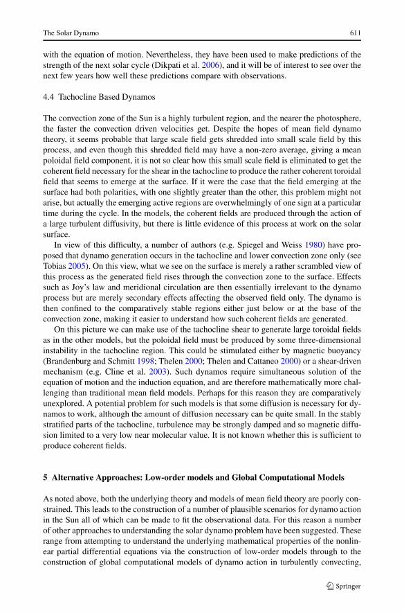
Fig. 1 Solar-cycle activity on the Sun since 1874. The lower panel shows the daily sunspot area, as a percent-age of the visible hemisphere that is covered by sunspots and averaged over individual solar rotations. Thebutterfly diagram in the upper panel shows the corresponding incidence of sunspots as a function of latitudeand time. At the beginning of a new cycle, spots appear around latitudes of ±30◦ . The activity zones spreaduntil they extend to the equator, and then gradually die away, disappearing at the equator as the first spots ofthe next cycle appear at higher latitudes (courtesy of D.H. Hathaway)

Fig. 1). Sunspots exist for anything from a few days to more than two solar rotation periods(i.e. more than two months). Early in the solar cycle, new sunspots occur preferentially atmid-latitudes on the Sun, and occur successively closer to the solar equator as the cycleprogresses. Plotting the locations of sunspots as a function of latitude and time thus givesrise to the so-called butterfly diagram (upper panel of Fig. 1).

Sunspots are cooler and darker than the rest of the solar photosphere (the visible surfaceof the Sun), with typical sunspot temperatures being 4000 K compared with the photo-sphere’s 6000 K. The outer 30 per cent by radius of the Sun constitutes the convection zone,where convective motions of the plasma transport heat from the deeper interior to the solarsurface. But the strong magnetic fields in sunspots inhibits the convective motions (a typicalstrength at the centre of a spot is 2–3000 G and the plasma beta is of order unity), causingthe spots to be cooler and hence darker. Actually the structure of a sunspot is rather com-plex and beautiful, with a dark inner region known as the umbra and a surrounding regioncalled the penumbra which exhibits a filamentary structure and is quite dynamic, as revealedfor example by the exquisite observations from the Hinode satellite (e.g. Jurcak and BellotRubio 2008).

Further work by Hale and his collaborators (Hale et al. 1919) concerning the polarity ofsunspot magnetic fields and their distribution and orientation in pairs established the basisfor what are now known as Hale’s Laws and Joy’s Law. Sunspots occur in bipolar pairsconsisting of a leading spot and a trailing spot, aligned approximately parallel to the solarequator. Hale’s Laws are that the magnetic polarities of the leading and trailing spot in apair are opposite, with the polarities being reversed in the two hemispheres; and that thepolarities reverse in successive solar cycles. Joy’s Law is that the line joining leading andtrailing spots in a pair tends to be inclined at an angle of about 4◦ to the equator. Takingthe change in polarity into account, it is seen therefore that the quasi-period of the Sun’smagnetic cycle as revealed by sunspots is about 22 years.

The Solar Dynamo 593

As a theoretical aside, we may note the generally accepted theoretical picture is thatbipolar sunspot pairs are caused by toroidal field in the form of magnetic flux tubes ris-ing through the convection zone and forming so-called Omega loops. These loops emergethrough the surface, the two regions of intersection of the loops with the photosphere beingidentified with the bipolar sunspot pair (e.g. Fan 2004).

Sunspots typically occur within larger magnetic complexes called active regions. There isa reported tendency for active regions to recur at the same longitudinal position on the Sunduring a solar cycle and even from one cycle to another: these locations are called activelongitudes. Above active regions one observes magnetic loops or arcades of loops in theoverlying chromosphere and in the corona which is the outer atmosphere of the Sun. Theseloops are made manifest by emission from the plasma confined within them. Occasionalexplosive reconfigurations of these magnetic structures, caused by magnetic reconnection,give rise to flares and coronal mass ejections (CMEs).

As well as the sunspot fields, there is magnetic field on a wide range of smaller scales.Smaller bipolar structures called ephemeral regions appear at all latitudes and show littlecycle variation. A discovery of recent years is that the Sun has a lot of small scale magneticflux that has been dubbed the solar ‘magnetic carpet’. The flux that comprises the magneticcarpet is constantly emerging and disappearing (by subduction or reconnection), such thatthe magnetic carpet is renewed over a timescale of order one day. Whether this magneticflux is the product of local small-scale dynamo action or whether it is recycled old magneticflux is a matter of debate.

The Sun also possesses a weak (of order 1–2 G) global magnetic field that is predomi-nantly dipolar. In the polar regions, the global field rises to around 10 G. Like the sunspotfield, the polar field reverses its polarity roughly every 11 years. The polar field reversaloccurs at about the time that the azimuthal sunspot field reaches its peak strength, at about15–20◦ latitude (Parker 2007).

It may be noted that other observables that are related to the solar magnetic field also varyover the solar cycle: these include the 10.7 cm radio flux and the solar irradiance (particularlyat short UV wavelengths).

Solar-cycle studies can be extended further back in time using proxy data. The magneticfield from the Sun deflects galactic cosmic rays. In the Earth’s atmosphere these rays produceradioactive isotopes such as 14C, which is preserved in trees, and 10Be, which is preserved inpolar ice-caps. The abundances of these isotopes therefore vary in antiphase with the solarmagnetic field. Studies of both the ice-core record and tree-ring data allow the 11-yr cycleto be traced back over hundreds of years, while its envelope modulation can be traced backover millennia (see for example the review by Weiss and Thompson 2009).

From about 1645 to 1715, soon after Galileo had made the first telescopic studies ofsunspots, there were very few sunspots seen on the solar disc and those that were seenwere almost all in the Sun’s southern hemisphere. This period is known as the MaunderMinimum (Eddy 1976; Ribes and Nesme-Ribes 1993). Thus in this period the sunspot cycleseems to be broken. Yet ice-core studies show that a cyclical modulation continued throughthe Maunder Minimum, indicating that the Sun’s large-scale magnetic field continued eventhough there were few sunspots (Beer et al. 1998). The north-south symmetry of the sunspotdistribution was soon re-established after the end of the Maunder Minimum.

Studies of the proxy datasets indicate that the Maunder Minimum is only the latest of thegrand minima that have occurred in solar activity over time. Conversely, the present era ofrather large-amplitude solar cycles (cf. Fig. 1) is a grand maximum, though this is perhapsnow coming to an end (Abreu et al. 2008).

594 C.A. Jones et al.

1.2 Solar Rotation and Helioseismology

It is generally accepted that the strong toroidal field that gives rise to sunspots is producedby a large-scale dynamo. Differential rotation of the solar plasma is likely an importantingredient of that dynamo. The Sun’s rotation at the surface can be observed directly byspectroscopic Doppler measurements and by observing the motion of sunspots and othertracers. These observations show that the surface rotation period at the solar equator is about25 days, increasing with latitude to more than a month at high latitudes. There is somevariation in the periods obtained from different methods of measurement (see Beck 1999 fora comprehensive review).

In recent years helioseismology has provided a unique view of conditions in the solarinterior, including how the rotation varies with depth and latitude. Global helioseismologyuses observations of global resonant oscillations of the Sun. These modes are set up by es-sentially acoustic waves, which are generated by convective turbulence in the upper partof the convection zone and which bounce around in the solar interior. Because the Sun isnearly spherical, the horizontal structure of the modes thus formed is described by spher-ical harmonics, and the resonant frequencies are determined by the properties of the solarinterior. Rotation of the solar interior causes the modes set up by eastward- and westward-propagating waves to have slightly different frequencies. After measuring this ‘frequencysplitting’ for modes that are sensitive to different ranges of latitude and depth within thesolar interior, inverse techniques can be used to infer how the rotation varies with latitudeand depth. Moreover, measurements at different times reveal small temporal variations inthe rotation rate over periods of months and years.

Energy is generated by fusion reactions in the inner core of the Sun. This energy istransported outwards through the inner 70 percent of the solar interior by radiative transport,and thereafter by convective heat transport until one approaches very close to the surface.Helioseismology has demonstrated that the transition to convective heat transport whichwe refer to as the base of the convection zone, is located at a fractional radius r/R� =0.713 ± 0.003 (where R is the radius of the Sun) (Christensen-Dalsgaard et al. 1991; Basu1998). The location of the base of the convection zone appears to be independent of latitude(Basu and Antia 2001).

The above measurement refers to the location of the essentially adiabatically stratifiedenvelope, which may include a region of convective overshooting where the motions aresufficiently rapid to establish an adiabatic thermal stratification. The extent of overshootingis relevant to dynamo models, since an overshoot region may provide a place where magneticflux is stored and amplified before rising to the surface. Modelling of the convection in starssuggests that beneath the adiabatically stratified overshoot region there will be a rather sharptransition to subadiabatic stratification: if that is the case, helioseismology indicates that theextent of such overshooting is small, probably no more than one tenth of the pressure scaleheight (Basu and Antia 1994; Monteiro et al. 1994; Christensen-Dalsgaard et al. 1995).A larger extent of overshooting would be consistent with the seismology if the transitionwere smoother: such a model has been proposed by Rempel (2004).

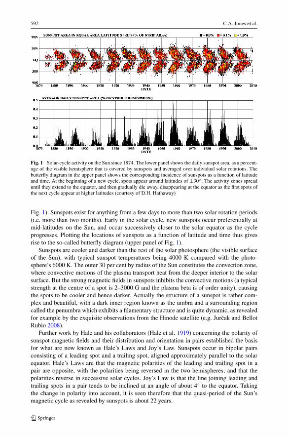
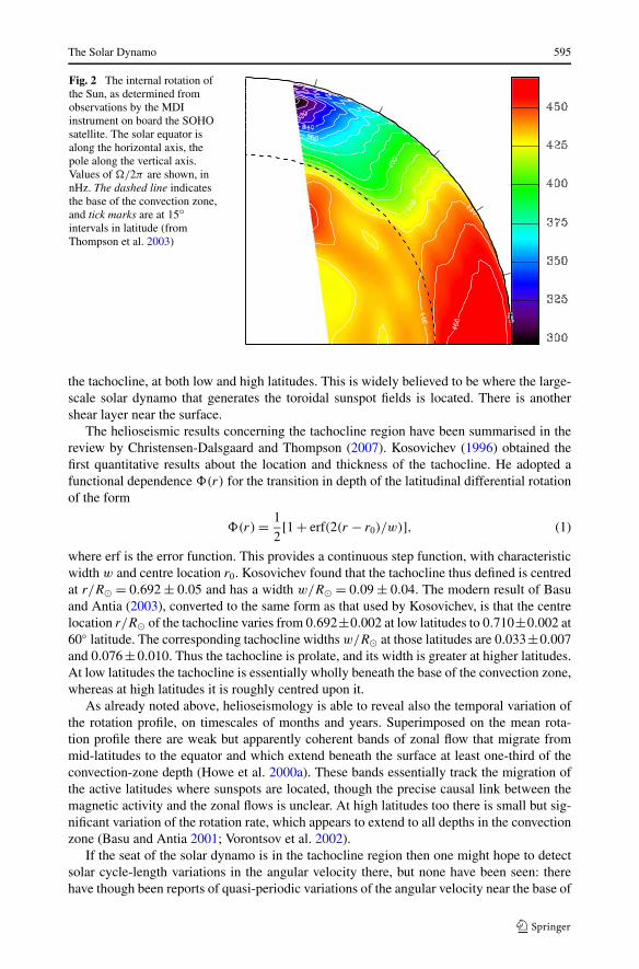
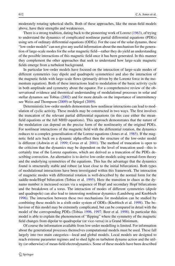
Helioseismology has determined the rotation profile of a substantial part of the solar in-terior: this is illustrated in Fig. 2. Beneath the base of the convection zone the solution isconsistent with solid-body rotation, whereas in the convection zone itself there is a differ-ential rotation with faster rotation at low latitudes and slow rotation in the polar regions.The rotation rate of the radiative interior matches the envelope rotation rate at mid-latitudes.There is thus a region of shear flow near the base of the convection zone, which is known as

The Solar Dynamo 595

Fig. 2 The internal rotation ofthe Sun, as determined fromobservations by the MDIinstrument on board the SOHOsatellite. The solar equator isalong the horizontal axis, thepole along the vertical axis.Values of �/2π are shown, innHz. The dashed line indicatesthe base of the convection zone,and tick marks are at 15◦intervals in latitude (fromThompson et al. 2003)

the tachocline, at both low and high latitudes. This is widely believed to be where the large-scale solar dynamo that generates the toroidal sunspot fields is located. There is anothershear layer near the surface.

The helioseismic results concerning the tachocline region have been summarised in thereview by Christensen-Dalsgaard and Thompson (2007). Kosovichev (1996) obtained thefirst quantitative results about the location and thickness of the tachocline. He adopted afunctional dependence �(r) for the transition in depth of the latitudinal differential rotationof the form

�(r) = 1

2[1 + erf(2(r − r0)/w)], (1)

where erf is the error function. This provides a continuous step function, with characteristicwidth w and centre location r0. Kosovichev found that the tachocline thus defined is centredat r/R� = 0.692 ± 0.05 and has a width w/R� = 0.09 ± 0.04. The modern result of Basuand Antia (2003), converted to the same form as that used by Kosovichev, is that the centrelocation r/R� of the tachocline varies from 0.692±0.002 at low latitudes to 0.710±0.002 at60◦ latitude. The corresponding tachocline widths w/R� at those latitudes are 0.033±0.007and 0.076 ± 0.010. Thus the tachocline is prolate, and its width is greater at higher latitudes.At low latitudes the tachocline is essentially wholly beneath the base of the convection zone,whereas at high latitudes it is roughly centred upon it.

As already noted above, helioseismology is able to reveal also the temporal variation ofthe rotation profile, on timescales of months and years. Superimposed on the mean rota-tion profile there are weak but apparently coherent bands of zonal flow that migrate frommid-latitudes to the equator and which extend beneath the surface at least one-third of theconvection-zone depth (Howe et al. 2000a). These bands essentially track the migration ofthe active latitudes where sunspots are located, though the precise causal link between themagnetic activity and the zonal flows is unclear. At high latitudes too there is small but sig-nificant variation of the rotation rate, which appears to extend to all depths in the convectionzone (Basu and Antia 2001; Vorontsov et al. 2002).

If the seat of the solar dynamo is in the tachocline region then one might hope to detectsolar cycle-length variations in the angular velocity there, but none have been seen: therehave though been reports of quasi-periodic variations of the angular velocity near the base of

596 C.A. Jones et al.

the convection zone with a period of 1.3–1.4 yrs (Howe et al. 2000b). It is interesting thoughthat there are apparent small changes in the wave speed near the base of the convection zonewhich are well correlated with solar activity (Baldner and Basu 2008; see also Serebryanskiyand Chou 2005).

One further dynamical ingredient that may be important to the operation of the solar dy-namo, as for example in the flux-transport dynamo models reviewed by Dikpati and Gilman(2009), is the north-south meridional circulation. Such flows have been measured in thenear-surface layers using local helioseismic techniques: the flows are poleward and largelysteady over a timescale of years. In the outer two per cent or so of the solar radius, the pole-ward flow speed is about 20–30 m s−1 and independent of depth (Haber et al. 2002). There isalso evidence that in the approach to the last solar maximum the flow in the northern hemi-sphere developed a counter-cell at mid-latitudes. Unfortunately, the helioseismic evidencefor what the meridional circulation is at greater depths is as yet inconclusive.

2 Modelling the Solar Dynamo

The observations discussed in the previous section demonstrate that stellar magnetic fieldsdisplay variability on an extremely wide range of space and time scales. Thus the modellingof the dynamics of this magnetic field must be able to identify the processes that lead todynamo action on these scales and formulate the mechanisms by which these scales caninteract, or at least attempt to parameterise the effects of the scales that have not been in-cluded in the theory. This is a difficult task. Essentially, as we shall argue below, the levelof turbulence in solar and stellar interiors leads to extreme parameter regimes in which thetheory must be applied and makes progress extremely slow.

2.1 Difficulties for Dynamo Modelling: The Solar Parameter Regime

The equations that govern magnetic field generation in the solar and stellar interiors arewell-known. Essentially they take the form

ρ(∂tu + u · ∇u + 2� × u)

= −∇p + 1

μ0(∇ × B) × B + μ

(∇2u + 1

3∇(∇ · u)

)+ F, (2)

∂tB = ∇ × (u × B) + η∇2B, (3)

∂tρ + ∇ · (ρu) = 0, (4)

∇ · B = 0, (5)

where ρ is the density of the plasma, u is the velocity, B is the magnetic field, μ0 is thepermeability of free space, � is the rotation vector and F is the forcing in the momentumequation that drives the fluid flow. Here μ is the dynamic viscosity and η is the magneticdiffusivity, both assumed constant. In general in stellar interiors the driving is from buoyancyforces that lead to thermally driven convection. Hence for a self-consistent solution, themomentum equation and induction equation above must be coupled to an energy equationand an equation of state (where usually the plasma is taken to be an ideal gas in whichp = RρT , with T the temperature and R the gas constant).

Given that the equations for magnetic field generation via fluid flow are well-known,the difficulties in describing the field generation processes occur owing to the fact that it is

The Solar Dynamo 597

Table 1 Typical values of dimensionless parameters in the Sun

Base of convection zone Photosphere

Rayleigh number Ra = gαβL4ρ/κμ 1020 1016

Reynolds number Re = UL/ν 1013 1012

Magnetic Reynolds number Rm = UL/η 1010 106

Prandtl number Pr = ν/κ 10−7 10−7

Magnetic Prandtl number Pm = ν/η 10−3 10−6

Rossby number Ro = U/2�L 0.1–1 10−3–0.4

Ekman number Ek = ν/2�L2 10−14 10−15–10−13

Mach number M = U/cs 10−4 1

Here g is the local gravity, α the thermal expansion coefficient, β is the superadiabatic temperature gradient,and κ the thermal diffusivity

impossible directly to solve these equations in the parameter regimes that occur in stellarinteriors with the current computational resources. As for planetary and geodynamo theory,the difficulties arise because one or more of the non-dimensional parameters is extremelylarge. However for dynamo theory relating to field generation in moderately rotating stars,the difficulties arise in different places in the equations than for planetary models. The re-view of the solar dynamo by Ossendrijver (2003) gives estimated numerical values for therelevant non-dimensional parameters both at the base of the solar convection zone and at thephotosphere (the visible surface). These are included in Table 1 for completeness.

The set of equations described above together with the parameter set detailed in Table 1in theory give all the information necessary to determine the dynamics. As noted above thedifficulties in determining the dynamics of magnetic fields in stellar interiors are manifestedin different ways to those for the interiors of planets. By far the most troublesome of theseparameter values for the solution of the dynamo system is the extreme values of the fluidand magnetic Reynolds numbers, Re and Rm. The large Reynolds number ensures thatthe flows that drive the dynamo are extremely turbulent with a large range of spatial andtemporal scales. These are largely unconstrained and interact in highly nonlinear manner.Perhaps more troubling from a dynamo perspective, is that the magnetic Reynolds numberin this turbulent environment remains extremely large, leading to the efficient generationof magnetic fields on extremely small scales, as we shall see. This is in contrast to theenvironment in planetary interiors where although the fluid Reynolds number is usually largeand the flow turbulent, the flow is constrained by rotation (which itself provides a problemfor modellers). Moreover in planetary interiors Rm is moderate (probably only a few timesabove critical) and so the process of field generation can be explored in the correct parameterregime. In short, whilst the modelling of planetary dynamos is plagued by the inability to getthe correct magnetostrophic balance in the momentum equation, solar and stellar dynamotheorists are still arguing about the correct solutions to the turbulent induction equation!

2.2 Large and Small Scale Dynamo Action

The observations described in the introduction were focused on the behaviour of the system-atic global solar magnetic field. High resolution observations of the magnetic fields in theSun also reveal the existence of small-scale unsystematic magnetic fields at the solar sur-face (e.g. Régnier et al. 2008), the dynamics of which appears to be largely decoupled fromthat of the solar cycle. This “magnetic carpet” is also believed to be generated by dynamo

598 C.A. Jones et al.

action—convective motions at the solar surface lead to the generation of fields there. Thescale of these fields is comparable with or smaller than the largest scale convective motions.This co-existence of magnetic fields on a wide-range of scales with very different propertieshas led to the separation of solar dynamo theory into two strands, small-scale dynamo the-ory (sometimes termed fluctuation dynamo theory) in which the field is generated on scalessmaller (or of the same size) than those of the turbulent eddies, and large-scale dynamo the-ory, which is concerned with the systematic generation of fields at a scale larger than thatof the turbulence. It is not clear that this distinction between large and small-scale dynamosis at all useful. However, historically a different range of techniques has been applied to thetwo problems and for this reason they have remained largely separated.

The bulk of this article is concerned with the theory for the generation of the systematicsolar activity cycle. However we begin by discussing recent advances in small-scale turbu-lent dynamo theory (see Tobias 2009 for a more thorough discussion). It is fair to say thatmuch more is understood about the dynamics of small-scale dynamos than large-scale ones.The dramatic recent increase in computational power coupled with the development of effi-cient numerical algorithms have led to major breakthroughs in our understanding. Numericalsimulations of turbulent dynamos driven by Boussinesq convection (see e.g. Cattaneo 1999;Cattaneo and Hughes 2006; Tobias et al. 2008) have demonstrated that this turbulentflow is capable of generating small-scale magnetic field if the magnetic Reynolds num-ber Rm—the non-dimensional measure of the rate of stretching to diffusion—is largeenough. A number of local models have followed these initial calculations. The role of com-pressibility has been included in a number of models (see e.g. Stein and Nordlund 2002;Vögler and Schüssler 2007). It has been suggested that strong stratification can inhibit dy-namo action (Stein and Nordlund 2002) although it appears that this is not the case, pro-viding the magnetic Reynolds number is large enough. The role of shear, penetration androtation in modifying small-scale dynamos has also been systematically investigated (Tobiaset al. 2008). There is also still some doubt as to whether a small-scale dynamo can operatewhen the fluid Reynolds number Re is much larger than Rm, the so-called small magneticPrandtl number limit—the appropriate limit for the solar interior. Although this issue is notsettled (and is exceedingly difficult to settle via numerical computation, see e.g. Iskakov etal. 2007) the indications are that these small-scale dynamos can survive efficiently in thislimit (Boldyrev and Cattaneo 2004; Tobias and Cattaneo 2008).

One consistent result that emerges from these simulations is that for high magneticReynolds number dynamos (i.e. ones for which Rm � Rmc with Rmc the critical value)the field that is generated is dominated by small scales—even in the presence of rota-tion, although the simulations are capable of generating systematic fields when Rm isclose to its critical value (see e.g. Brandenburg et al. 2008, Käpylä et al. 2008). Thisis an important result and has been discussed in detail (Cattaneo and Hughes 2006;Hughes and Cattaneo 2008). The apparent predominance of small-scale magnetic fields athigh Rm in turbulent flows is a central problem of turbulent dynamo theory and is an issuethat we shall return to in our discussion of large-scale field generation below.

2.3 Physical Effects and Approaches to Modelling the Solar Dynamo

For the rest of this article we discuss the current status of the theory for the generation ofthe systematic global solar field. The theory has developed from along a number of parallelstrands, utilising a combination of basic theory, turbulence modelling and numerical compu-tation. The range of approaches will be outlined below, before a detailed discussion of eachin subsequent sections. In this section we discuss the basic physical effects that can lead tosystematic dynamo action.

The Solar Dynamo 599

Conceptually it is convenient to discuss the dynamics of a global (large-scale) axisym-metric magnetic field. It is then possible to decompose the field (in spherical polar co-ordinates) into toroidal and poloidal parts so that B = Bφeφ + ∇ × (Aeφ); here Bφ(r, θ)

is the toroidal (zonal) field and A(r, θ) is the vector potential for the poloidal (meridional)field. It is well known that the presence of differential rotation uφ(r, θ) naturally leads tothe generation of Bφ from A—toroidal field is generated efficiently from poloidal field viagradients in angular velocity. This action of differential rotation is often termed the �-effectand is uncontroversial. If this were the only ingredient of the dynamo then the axisymmetricfield would ultimately decay as demonstrated by Cowling (1933) in his famous anti-dynamotheorem. However in a landmark paper Parker (1955) argued that turbulent (small-scale)convective motions in the solar interior could produce small-scale (non-axisymmetric) mag-netic fields. Furthermore, he argued that the net effect of the small-scale flows interactingwith the small-scale magnetic fields could be so as to produce a net electromotive force(e.m.f.) that is capable of regenerating the axisymmetric poloidal field from the axisymmet-ric toroidal field. This non-trivial effect was formalised in the landmark paper of Steenbecket al. (1966) which introduced mean-field electrodynamics. This formalism has been the ba-sis of solar and stellar dynamo theory for more than forty years and has been investigated indetail (as described in the next section).

Although much attention has focused on the mean-field formalism (both in terms ofexamining the applicability and the consequences of the theory) other approaches to thedynamo problem have been investigated. The breathtaking advances in computational re-sources and algorithms have enabled the construction of global dynamo models which, al-though in parameter regimes many orders of magnitude away from the conditions inside astar, are beginning to give insights into the operation of stellar dynamos. These global mod-els are reviewed in Sect. 5. A final approach is to use the techniques of nonlinear dynamicsand bifurcation theory to investigate the mathematical structure of the underlying equationsand to construct simple (low-order) models that lead to an understanding of the possiblecomplicated dynamics of stellar dynamos. These models will also be discussed in Sect. 5.

3 Mean Field Dynamos: Theory

The subject of mean-field dynamo theory can be divided into two main areas. First, there isthe theory itself, the conditions under which it is valid, its relationship to turbulence theory,and its extension to include nonlinear effects. Second, there are the applications of mean-field dynamo theory, the solar and stellar models that have been developed using the α-effectterm in the induction equation, which is the essential new ingredient provided by the theory.There is surprisingly little interaction between these two areas of research. A vast body ofwork on α-effect dynamo models exists, using many different geometries, both with andwithout nonlinear terms in the equations, and with many different spatial locations of theα and � effects. In contrast, much less has been done on the fundamental assumptions un-derlying mean-field dynamo theory, so that it is still controversial to what extent the modelsusing mean-field concepts can be relied upon. As we see below, there are some clearly de-fined limits where mean-field dynamo theory is certainly correct, but unfortunately theselimits are very far from the conditions in the Sun, stars and galaxies where they are applied.This does not necessarily mean that mean-field dynamo theory gives wrong answers for as-trophysical dynamos, but it does mean that such theories cannot be relied on very strongly.They may suggest possible scenarios for the behaviour of stellar and galactic dynamos, andprovide a framework in which observations can be interpreted, but unlike Newton’s laws ofmotion, they cannot provide definite predictions of future behaviour.

600 C.A. Jones et al.

The theory developed in the 1960’s by Krause, Rädler and Steenbeck (see e.g. Krause andRädler 1980) was essentially a linear theory. Independently, Braginsky (1975) developed histheory of the nearly axisymmetric dynamo, which contains similar ideas, though based ona different averaging procedure. Vainshtein and Cattaneo (1992) questioned whether theclassical mean-field theory could survive intact when nonlinear effects were included. Theyargued that because of the very high magnetic Reynolds number in most astrophysical ob-jects, the α-effect would be quenched by the nonlinear effect of even rather small magneticfields, thus throwing into doubt the relevance of the α-effect model in astrophysics. Sub-sequently, this negative result has been questioned, but the whole issue of the reliability ofthe α-effect model is still controversial. To date there has not been much support for mean-field dynamo theory from direct numerical simulations of the MHD equations. Proponentsof mean-field theory correctly point out that these numerical simulations are not in the astro-physical parameter regime either, but nevertheless it remains a matter of concern that thereis so little agreement between these two main lines of research into dynamo theory.

3.1 Averaging the Dynamo Equations

The basic idea of mean-field theory is to split the magnetic field and the flow into mean andfluctuating parts,

B = B + B′, u = u + u′. (6)

The mean part is thought of as the large scale average field and velocity, the fluctuating partis thought of as a small scale turbulent contribution. We also need an averaging procedure,discussed in more detail in Sect. 3.2 below. The fundamental property of the averaging is thatthe fluctuating quantities on their own average to zero, but products of fluctuating quantitiescan have a non-zero average. So

B′ = u′ = 0. (7)

However the averaging process is defined, it must obey the averaging rules, that is the sumof the average of a number of terms must be the average of their sum, averaging commuteswith differentiating both with respect to space and time, and averaging an averaged quantityleaves it unchanged. There are several different ways of defining the average. If the turbu-lence is small-scale and the mean field we are interested in is large-scale, then there is scaleseparation. We can average over an intermediate length-scale

F(x, t) =∫

F(x + ξ, t), g(ξ) d3ξ,

∫g(ξ) d3ξ = 1. (8)

We choose the weight function g to go to zero at large distances on the intermediate lengthscale, but g is constant over small distances, so fluctuations average out but mean fielddoesn’t, ∫

F ′(x + ξ, t) g(ξ) d3ξ = 0,

∫F(x + ξ, t)g(ξ) d3ξ = F . (9)

Braginsky (1975) suggested another method of averaging, over a coordinate, usually theazimuthal angle φ in spherical systems. So then B is just the axisymmetric part of the field.In Cartesian models, with gravity and possibly rotation in the z-direction, it is common todefine the average over both the horizontal coordinates so that B is a function of z only.This method of defining the average has become more popular recently, as it is suited to

The Solar Dynamo 601

comparison with simulations. It is quite different from the scale separation method of defin-ing the average; in general the nonaxisymmetric components of the flow will have a similarlength-scale to the axisymmetric components.

We now insert (6) into the induction (3) and average to obtain the mean-field inductionequation

∂B∂t

= ∇ × (u × B) + ∇ × (u′ × B′) + +η∇2B. (10)

Note that the terms involving products of a mean and a fluctuating quantity average to zero,but crucially the term involving products of fluctuating quantities can have a non-zero meanpart. The fluctuating field B′ and the fluctuating turbulent part of the velocity u′ can besystematically aligned to give a non-zero mean e.m.f.

E = u′ × B′. (11)

The great advantage of this new mean e.m.f. term in the mean induction equation (10) isthat Cowling’s theorem no longer applies, so we can find simple axisymmetric dynamos assolutions. This releases us from the constraint of having to solve fully three-dimensionalsolutions of the dynamo equations, which invariably involve the construction of complexnumerical computer programs, which is both difficult and time-consuming. In view of this,it is not surprising that most work on dynamo theory has used the mean field equationswith a non-zero mean e.m.f. The mean e.m.f. term creates poloidal field from toroidal field,and hence closes the dynamo loop. We already have the differential rotation stretching outpoloidal field into toroidal field, and the mean e.m.f. gives a mechanism for converting thattoroidal field into new poloidal field. However, to exploit this we must have a rational wayof determining what the mean e.m.f. actually is.

3.2 Evaluation of the Mean e.m.f.

If we subtract the mean-field equation (10) from the full equation (3), we obtain the equationfor the fluctuating field B′,

∂B′

∂t= ∇ × (u × B′) + ∇ × (u′ × B) + ∇ × G + η∇2B′,

G = u′ × B′ − u′ × B′.(12)

There are a number of different approaches to dealing with this equation. In the classicalmean-field approach, Krause and Rädler (1980), we view u′ as a given turbulent velocityindependent of B′ and B. In the Braginsky (1975) approach, the equation of motion is lin-earised, and u′ and B′ are solved simultaneously. It is also possible to make assumptionsabout the relation between u′ and B′ through the equation of motion, one such being theEDQNM model (Pouquet et al. 1976), referred to again in Sect. 3.6 below.

In the classical mean-field approach, u′ is given so (12) is a linear equation in B′ with aforcing term ∇ × (u′ × B). There are then two possibilities. Equation (12) may have non-trivial solutions when B = 0, in which we say there is a small-scale dynamo. The alternativeis that there is no small-scale dynamo, in which case B′ → 0 as t → ∞ if B = 0. If thisis the case, B′ will be entirely created by the forcing from the action of the turbulence onthe mean field. Then B′(x) will be proportional to B, but only if the turbulence has a shortcorrelation length will B′(x) depend on only the local value B(x), more generally it will be

602 C.A. Jones et al.

a non-local dependence, i.e. involving an integral containing B(x′). However, if there is ashort correlation length, we can evaluate B′ and hence E as a Taylor series

Ei = E 0i + aij Bj + bijk

∂Bk

∂xj

+ · · · , (13)

where the tensors aij and bijk depend on u′ and u and the term E 0i is driven by the small-

scale dynamo, if any. This equation is really the essence of mean-field dynamo theory. Aswe see below, it usually further assumed that the tensors appearing in (13) are isotropic, andit is this equation which forms the basis of the vast majority of mean-field dynamo models.

Many assumptions have gone into deriving this key result (13). When are they likely to bevalid? The first assumption was that u′ is given. It is now widely recognised that actually itwill be affected by B′ and B. This leads to α-quenching, discussed in more detail in Sect. 3.6below. If there is a small-scale dynamo, then B′ can grow independently of any mean field,and will reach a level such that the small-scale Lorentz force affects the small-scale flowsufficiently to prevent further growth. This leads to the zeroth order term E 0

i in (13), whosepossible form was discussed by Rädler (1976) and subsequently by Yoshizawa et al. (2000),see also references therein. In most applications, however, this zeroth order term is omitted.

In the original concept of mean-field dynamo theory, it was envisaged there would bescale separation, in which case the appropriate length scale for the fluctuating field is notthe integral scale d of the whole dynamo region, but the much smaller turbulent correlationlength, say �. Now Rm′ = u′�/η, and there is some hope that Rm′ will be too small to allowa small-scale dynamo, but Rm = ud/η is large enough to allow large-scale field to grow.Under these circumstances, B′ is simply linearly forced by B, and mean-field theory withE 0

i = 0 will be valid. So when may we expect scale separation to occur? Unfortunately notin the Sun, because the observational evidence suggests that turbulence occurs in the formof ‘granules’, flows that last some minutes of time and with a spatial scale of 103 km, whichwould give a large Rm′; not as large as the Rm for the whole Sun, but still large enoughto generate a small scale magnetic field by dynamo action. There is not much evidence ofscale separation in simulations either, with the possible exception of very rapidly rotatingconvection (Stellmach and Hansen 2004). Here tall thin convecting columns of fluid canoccur, in which the horizontal scale is significantly less than the vertical scale, but this isunlikely to be the case in the Sun, which rotates comparatively slowly. It is therefore notusually possible to justify applying mean-field dynamo theory to the solar dynamo in anyrigorous sense. It may be that mean-field models still have relevance to the Sun even thoughscale separation does not occur, but we must treat any mean field results with caution. To bebelievable, there must be strong, independent evidence supporting such models.

3.3 Tensor Representation of E

We now consider the possible forms of the tensors occurring in (13).aij tensor: we split this into a symmetric part (aij + aji)/2 = αij and the antisymmetric

part, (aij − aji)/2 = εijkAk . Then from this tensor we obtain

E = αij Bj − A × B. (14)

We already have a term u × B in the induction equation (10), so the A term just modifiesthe mean velocity. Along the principal axes, the symmetric part in general has 3 differentcomponents, but for isotropic turbulence

αij = αδij , (15)

The Solar Dynamo 603

leading to the usual mean-field α-effect dynamo equation,

∂B∂t

= ∇ × (u × B) + ∇ × αB + +η∇2B. (16)

bijk tensor: first we split the tensor ∂j Bk into symmetric and antisymmetric parts, so

∂j Bk = (∇B)s − 1

2εjkm(∇ × B)m. (17)

The symmetric part is believed to be less important than the antisymmetric part. The an-tisymmetric part combines with bijk to give a second rank tensor bijkεjkm (the summationconvention applies), and this second rank tensor has a symmetric and an antisymmetric part,giving

Ei = −βij (∇ × B)j − εijkδj (∇ × B)k. (18)

The δ-effect term has been discussed (e.g. Krause and Rädler 1980), but most interest hasfocused on the β-effect, especially the case where the βij tensor is isotropic, βij = βδij , as itthen gives a term identical in form to the diffusion term. We can now write the mean e.m.f.in the form most commonly used in mean-field theory

E = αB − β∇ × B. (19)

If we further assume β is constant in space, we obtain

∂B∂t

= ∇ × (u × B) + ∇ × αB + (η + β)∇2B. (20)

The β-term just enhances the diffusivity from a laminar value η to a turbulent value η + β .It is normally argued that β � η, so the diffusivity is greatly enhanced by the turbulence.Of course it would be nice to use this enhanced diffusivity to claim that the small scaleturbulence does indeed have a low Rm′, but this is scarcely a logical argument, since scaleseparation was invoked to explain the appearance of the β term in the first place.

3.4 Helicity and the α-Effect

The tensor approach to mean-field dynamo theory leads to a large number of unknownquantities for the tensor components, which is rather unsatisfactory as one might suspectthat models with almost any desired property could be constructed by choosing these coeffi-cients sufficiently carefully. A more physical approach (Moffatt 1978) is to assume that theturbulence is a random superposition of waves

u′ = Re{u exp i(k · x − ωt)}. (21)

With short correlation lengths, the mean velocity term in the induction equation can beremoved by working in moving frame to give

∂B′

∂t= (B · ∇)u′ + ∇ × (u′ × B′ − u′ × B′) + η∇2B′,

O(B ′/τ) O(Bu′/�) O(B ′u′/�) O(ηB ′/�2).

(22)

604 C.A. Jones et al.

If the small-scale magnetic Reynolds number u′�/η is small, the awkward curl term is neg-ligible. This is the first order smoothing assumption,

∂B′

∂t= (B · ∇)u′ + η∇2B′. (23)

This implies B′ B, almost certainly not true in the Sun. Then inserting (21) into (23), weobtain

B′ = Re

{i(k · B)uηk2 − iω

exp i(k · x − ωt)

}. (24)

Now we can evaluate E ,

E = u′ × B′ = 1

2

iηk2(k · B)

η2k4 + ω2(u∗ × u), (25)

where ∗ denotes complex conjugate, equivalent to

αij = 1

2

iηk2

η2k4 + ω2kj εimnu

∗mun. (26)

For any particular wave, the α-tensor is not isotropic, but if we have a random collectionof waves with u and k in random directions, the sum of all the contributions to the α-effectwill be isotropic, so αij = αδij .

We now consider the helicity

H = u′ · ∇ × u′ = 1

2ik · (u∗ × u). (27)

Taking the trace of (26) gives

α = −1

3

ηk2H

η2k4 + ω2. (28)

So, under the first order smoothing approximation, the mean e.m.f. is proportional to thehelicity of the turbulence. Since helicity is the scalar product of velocity and vorticity, a flowwith non-zero helicity must consist of helical motion. If an element of fluid rises and rotatesabout the vertical as it does so, the flow has helicity. To obtain a non-zero α-effect, there mustbe a systematic bias to the rotation, for example if rising fluid in the northern hemispherepredominantly rotates clockwise, the net helicity is negative, so from (28), positive α isgenerated in the northern hemisphere. It is not required that every rising element of fluid inthe northern hemisphere rotates clockwise, only that on average more rotate clockwise thananticlockwise. This type of asymmetry is most easily generated by the effect of rotation onthe convection, and indeed rotating convection invariably produces non-zero helicity. It alsousually produces helicity of opposite sign in the two hemispheres, so most models of theα-distribution make it antisymmetric across the equator.

Another way of relating the helicity to the mean e.m.f. is to assume that the correlationtime of the turbulent fluctuating part is short, the so-called short sudden approximation. Nowin (22) the time-derivative term just balances the first term on the right provided u′ < �/τ ,and now we assume Rm′ large, so that the diffusive term is also negligible. Again assumingthe turbulence has no preferred direction, this leads to

α = −τ

3u′ · ∇ × u′ (29)

so again α is proportional to the helicity.

The Solar Dynamo 605

These results suggest that the value of α will be anticorrelated with helicity. However,they all assume either first-order smoothing or short sudden turbulence, neither of whichis easy to justify in solar conditions. Courvoisier et al. (2006) looked numerically at the α

produced by a variety of flows where neither of these assumptions applied, and found thatthere was no robust correlation of α with helicity. Instead, they found that α could evenchange sign as Rm′ varied. It seems that the relationship of helicity and α is quite modeldependent, and only in limits unlikely to apply in the Sun is the relation clear-cut. Schrinneret al. (2007) have also performed numerical simulations in the rapidly rotating case, and findthat the α-tensor (14) is highly anisotropic.

3.5 Helicity and the Parker Loop Mechanism

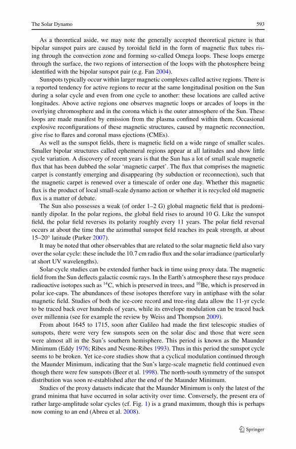
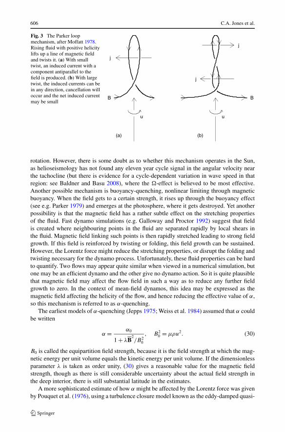
Despite the difficulties in justifying mean field theory and the α-effect in the Sun, observa-tions of sunspots and their associated magnetic active regions suggest that magnetic field isbeing brought to the surface by rising fluid coming up from below. A sunspot pair is createdwhen an azimuthal loop of magnetic field rises through the solar photosphere. The verticalfield impedes convection, reducing the heat transport and hence producing a relatively darkspot. Joy’s law, based on sunspot observations over a long time, says that sunspot pairs aresystematically tilted, with the leading spot being nearer the equator. Assuming flux was cre-ated as azimuthal flux deep down, this suggests that the loop has indeed twisted through afew degrees as it rose, and in a sense that implies negative helicity in the northern hemi-sphere. A rising loop of flux being twisted by helical motion is illustrated in Fig. 3a. Notethat the induced current is antiparallel to the original magnetic field. Parker (1955) realisedthe possible significance of this result, and it has subsequently become incorporated intomany dynamo models. Note that it is important that the amount of twist is small. If it is toogreat, as in Fig. 3b, the loop can be twisted through a large angle and the induced currentno longer simply points in the ‘correct’ direction. The currents induced are no longer coher-ent, and will average out to give only a negligible net current. In the first order smoothingapproximation, the B′ field generated by the turbulence is always small compared to theoriginal B field so the twist is necessarily small. Possibly the same effect is achieved in theSun by the field rising quite rapidly, so the field does not have time to rotate by more than asmall angle before it emerges at the surface. This suggests that it might be possible for meanfield theory to work in the Sun, even though the assumptions needed to guarantee its valid-ity do not hold. It is though less clear that this mechanism can generate α throughout theconvection zone, and indeed in many models, e.g. the Babcock-Leighton model (Leighton1969) and the Parker (1993) interface dynamo, the regions where the � and α effects occurare spatially separated.

3.6 Nonlinear Effects and α-Quenching

The mean-field induction equation (20) is linear in B, so it predicts fields either grow ordecay exponentially. To determine how the field saturates, and the field strength at whichthis occurs, we must include nonlinear effects. The only possible nonlinearity is the Lorentzforce in the equation of motion (2), though there are a number of different ways in whichthis term could achieve magnetic saturation. Perhaps the simplest is that the Lorentz forcecould act to stop the differential rotation, the �-quenching mechanism. Indeed, simulationsof convection in rotating fluids often show a large reduction in differential rotation oncea dynamo generated magnetic field permeates the fluid. The magnetic interior of the gasgiant Jupiter also appears to be rotating rather uniformly, in strong contrast to the non-magnetic outer regions where there are fast flowing jet flows, i.e. significant differential

606 C.A. Jones et al.

Fig. 3 The Parker loopmechanism, after Moffatt 1978.Rising fluid with positive helicitylifts up a line of magnetic fieldand twists it. (a) With smalltwist, an induced current with acomponent antiparallel to thefield is produced. (b) With largetwist, the induced currents can bein any direction, cancellation willoccur and the net induced currentmay be small

rotation. However, there is some doubt as to whether this mechanism operates in the Sun,as helioseismology has not found any eleven year cycle signal in the angular velocity nearthe tachocline (but there is evidence for a cycle-dependent variation in wave speed in thatregion: see Baldner and Basu 2008), where the �-effect is believed to be most effective.Another possible mechanism is buoyancy-quenching, nonlinear limiting through magneticbuoyancy. When the field gets to a certain strength, it rises up through the buoyancy effect(see e.g. Parker 1979) and emerges at the photosphere, where it gets destroyed. Yet anotherpossibility is that the magnetic field has a rather subtle effect on the stretching propertiesof the fluid. Fast dynamo simulations (e.g. Galloway and Proctor 1992) suggest that fieldis created where neighbouring points in the fluid are separated rapidly by local shears inthe fluid. Magnetic field linking such points is then rapidly stretched leading to strong fieldgrowth. If this field is reinforced by twisting or folding, this field growth can be sustained.However, the Lorentz force might reduce the stretching properties, or disrupt the folding andtwisting necessary for the dynamo process. Unfortunately, these fluid properties can be hardto quantify. Two flows may appear quite similar when viewed in a numerical simulation, butone may be an efficient dynamo and the other give no dynamo action. So it is quite plausiblethat magnetic field may affect the flow field in such a way as to reduce any further fieldgrowth to zero. In the context of mean-field dynamos, this idea may be expressed as themagnetic field affecting the helicity of the flow, and hence reducing the effective value of α,so this mechanism is referred to as α-quenching.

The earliest models of α-quenching (Jepps 1975; Weiss et al. 1984) assumed that α couldbe written

α = α0

1 + λB2/B2

0

, B20 = μρu2. (30)

B0 is called the equipartition field strength, because it is the field strength at which the mag-netic energy per unit volume equals the kinetic energy per unit volume. If the dimensionlessparameter λ is taken as order unity, (30) gives a reasonable value for the magnetic fieldstrength, though as there is still considerable uncertainty about the actual field strength inthe deep interior, there is still substantial latitude in the estimates.

A more sophisticated estimate of how α might be affected by the Lorentz force was givenby Pouquet et al. (1976), using a turbulence closure model known as the eddy-damped quasi-

The Solar Dynamo 607

normal Markovian approximation (EDQNM). As with all turbulence closure models, thereis no rigorous way of justifying such approximations, but they do use plausible assumptionsabout the statistical nature of the turbulence. Interestingly, they found (as did Gruzinov andDiamond 1994) that (29) is replaced by

α = −τ

3

(u′ · ∇ × u′ − 1

ρj′ · B′

). (31)

This formula includes the Lorentz force into the expression for α so that nonlinearity directlyreduces the effective α. Its range of validity has been discussed by Proctor (2003). Naturally,this expression for α again depends on some first order smoothing approximation or shortsudden approximation, as it gives the usual anticorrelation of α and helicity in the weak fieldlimit, questioned by Courvoisier et al. (2006).

In the early 1990’s, Vainshtein and Cattaneo (1992) suggested that at large magneticReynolds numbers the parameter λ in (30) should be O(Rm), not O(1). As Rm is verylarge in the Sun, there is a huge difference between these estimates, the Vainshtein andCattaneo estimate only allowing a very small mean field. Since there does seem to be alarge reasonably large coherent mean magnetic field, as evidenced by the solar cycle anddirect flux measurements, this very active α-quenching came to be known as catastrophicα-quenching. There has been much discussion of possible ways of avoiding the catastrophicα-quenching dilemma without abandoning the whole concept of mean-field dynamo theory.One way is to postulate that the regions where the α-mechanism operates are physicallydifferent from those where the �-effect occurs. Then it is possible that α operates where thefields are relatively small, so avoiding the strong quenching, but � operates in the strongfield region near the tachocline where α-quenching is irrelevant. This is the basic idea ofParker’s (1993) interface dynamo (see also Charbonneau and MacGregor 1997), and is alsopart of the philosophy of flux-transport dynamo models (Dikpati and Charbonneau 1995),though to avoid α-quenching, if it exists, very low values for the mean-field are required inthe convection zone.

3.7 Magnetic Helicity and α-Quenching

How does the catastrophic α-quenching come about? Vainshtein and Cattaneo (1992) per-formed numerical simulations which suggested λ ∼ Rm, but they also had a simple expla-nation of why this comes about. At large Rm fluid flow expels magnetic flux out of eddies,into the relatively stagnant regions between them. This is known as flux expulsion (Weiss1966). Galloway et al. (1977) showed that the resulting flux ropes have thickness Rm−1/2

times the integral length scale, and the field is much stronger in these ropes than in the meanfield. The Lorentz force in the dynamo process acts when there is local equipartition be-tween kinetic and magnetic energy, but this is when the locally very large fluctuating fieldis in equipartition with the kinetic energy. The mean field is then much smaller than theequipartition energy. The root of the problem is that at large Rm the fluctuating small scalefield is actually much larger than the mean field, not smaller as in the low Rm first ordersmoothing scenario. It is when this small scale field generates significant Lorentz force thatthe dynamo saturates.

Further insight into the nature of catastrophic α-quenching through the concept of mag-netic helicity was obtained by Gruzinov and Diamond (1994). Because ∇·B = 0, we canwrite

B = ∇×A, ∇·A = 0,

608 C.A. Jones et al.

where A is called the vector potential. The condition ∇·A = 0 is called the Coulomb gauge,and is necessary to specify A because otherwise we could add on the grad of any scalar. Wecan compute A explicitly from B using the Biot-Savart integral,

A(x) = 1

4π

∫y − x

|y − x|3 × B(y) d3y,

the integral being over all space. The induction equation in terms of A is then

∂A∂t

= (u × ∇×A) + η∇2A + ∇φ, ∇2φ = −∇·(u × B), (32)

and the magnetic helicity is defined as

Hm =∫

A · B d3x = 〈A · B〉, (33)

the integral being over the dynamo region, so the angle brackets denote the volume integral.The significance of magnetic helicity is that it is a conserved quantity in the non-dissipativelimit. In objects with large Rm, magnetic helicity will not be conserved exactly, but one mayexpect that it can only change relatively slowly, on a diffusive timescale possibly enhancedby turbulence. Using some vector identities, we obtain

⟨D

Dt(A · B)

⟩=

∫∇ · [B(φ + u · A)] + ∇ · [A × (η∇ × B)]d3x − 2ημ〈B · J〉. (34)

The first divergence term can usually be eliminated by defining φ suitably. The second diver-gence term gives a resistive surface term and can usually be ignored. So the total magnetichelicity is conserved if η is small (large Rm). The quantity B ·J is called the current helicity,and it too is of interest. There have even been some recent attempts to measure its value onthe solar surface (Sokoloff et al. 2008). In a steady state, (34) shows that the current helicitymust average to zero.

We now split the magnetic helicity into its mean and fluctuating parts and perform thesame manipulations as before (for details see e.g. Jones 2008, Sect. 5.3)

∂

∂tA′ · B′ = −2B · u′ × B′ − 2ημj′ · B′ + divergence terms (35)

so ignoring the divergence terms, which only involve surface effects, the small scale helicityalso decays because of the current helicity, but there is an additional term involving the meane.m.f. E = u′ × B′. This allows transfer between the small scale and large scale magnetichelicities. Now using (19) in a steady state

αB2 − μβB · J = −μη j′ · B′. (36)

There are two different ways of interpreting (36). If the length scale � of the fluctuations isshort compared to the mean field length scale d , the β term is O(�/d) compared to the α

term, so the β term can be ignored, and the balance is between the α term and the moleculardiffusion term on the right-hand side. In this case α is limited by the molecular diffusivityunless |B′| � |B|, the opposite of the normal assumption of mean field theory. Alternatively,one can argue that although the β term is nominally smaller than the α in mean-field theory,in practice the terms may be comparable, so the primary balance is between the α and β

The Solar Dynamo 609

terms in (36), with the diffusive term on the right-hand side being negligible. Then α islimited not by the very small inverse magnetic Reynolds number, but instead by �/d (e.g.Brandenburg and Subramanian 2005).

If the Lorentz force limits α by reducing the helicity, we might also expect the turbulentdiffusion to be reduced. This is called β-quenching, and it is currently an active researchtopic (e.g. Gruzinov and Diamond 1994; Petrovay and Zsargo 1998; Keating et al. 2008).These authors point out that if β quenching is significant, it is likely that β will be stronglyanisotropic. In view of the discussion above, if β is strongly quenched, then we may expectα to be strongly quenched also.

4 Mean Field Dynamo Models

4.1 Dynamo Waves

The simplest and perhaps the most instructive solutions of the mean-field equations are thedynamo waves (Parker 1955). Since we are no longer constrained by Cowling’s theoremand the related antidynamo theorems, growing waves in two dimensions are possible. Wecan therefore look for axisymmetric dynamos. We can even simplify further by adopting alocal Cartesian model with the y-coordinate representing the azimuthal direction φ. Then

B = (−∂A/∂z,B, ∂A/∂x), u = (−∂ψ/∂z,uy, ∂ψ/∂x) (37)

and the induction equation can be split into a ‘meridional’ part

∂A

∂t+ ∂(ψ,A)

∂(x, z)= αB + η∇2A, (38)

and an ‘azimuthal’ part

∂B

∂t+ ∂(ψ,B)

∂(x, z)= ∂(A,uy)

∂(x, z)− ∇ · (α∇A) + η∇2B. (39)

The simplest case is when ψ = 0, and α is constant, and the flow uy = U′ · x, a constantshear. Then waves A = exp(σ t + ik · x) are possible, and the dispersion relation is

(σ + ηk2)2 = iαy · U′ × k + α2k2. (40)

If the shear is zero, and provided α is large enough to overcome diffusion, this gives growingand decaying stationary solutions known as the α2 dynamo, while if the shear dominates andthe α2 term is comparatively small, there are also growing and decaying solutions known asthe α� dynamo. Naturally, the growing solutions dominate and eventually the field saturatesdue to some form of α-quenching as discussed above. The main solar magnetic field prop-agates towards the equator during the cycle, so almost all mean-field solar dynamo modelsare of α� type as these give propagating waves rather than a steady dynamo. The dimen-sionless combination D = α|U′|d3/η2 where d is a typical size of the dynamo region (oftentaken as the depth of the convection zone) is called the dynamo number, and in confinedgeometry there is a critical D which must be exceeded for onset.

Note that it is only the component of shear perpendicular to the wavevector k that candrive an α� propagating dynamo wave. So if we want dynamo waves propagating towardsthe equator, as observed in the solar cycle, we need a shear in the radial direction. Also, if

610 C.A. Jones et al.

the product of α and the shear has the wrong sign, the growing dynamo wave may propagatetowards the poles rather than the equator. Actually, at high latitudes, there is some evidenceof poleward waves, which might be explained in mean-field terms by a change in the signof α near the equator, or alternatively by a change in the sign of the shear. The need forradial shear to give latitudinal wave propagation has focused attention on regions of theSun which have a strong radial shear. There are two such regions, the tachocline and theshallow region immediately below the photosphere. Most models place the shear in thetachocline, but not all, see Brandenburg (2005). The theory is not changed greatly when wemove into axisymmetric spherical shell geometry, and it is possible to get models with themain features of the solar dynamo provided the shear and the distribution of α are chosenappropriately.

4.2 Interface Dynamo

Parker (1993) suggested that the shear occurred in the tachocline and the α-effect in theconvection zone. This separation is desirable because then the strong fields in the tachoclinemight not suppress the α-effect in the convection zone so much, and the tachocline is knownto be a region of strong shear. It also seems broadly consistent with the twisting of risingflux tubes in the convection zone being responsible for the α-effect. Numerical models withplausible α-distributions, with e.g. a latitudinal dependence cos θ sin2 θ (see e.g. Chan et al.2008 for a recent interface model dynamo) can lead to models which give a solar-like but-terfly diagram. This is encouraging, but generally the results to date do seem to be ratherdependent on the form of α selected; for example Markiel and Thomas (1999) found thatwith a latitudinal dependence cos θ and a differential rotation profile consistent with helio-seismology, it was difficult to obtain a realistic butterfly diagram.

4.3 Flux Transport Dynamos

These models go back to the ideas of Babcock (1961) and Leighton (1969), and are simi-lar to the interface dynamo concept, in that they are α� dynamos in which the shear is inthe tachocline while the α-effect is in the convection zone, and indeed may be due to theobserved twisting of field in line with Joy’s law. So far, this is quite similar to the interfacedynamo, but the new feature of flux transport dynamos is that the poloidal flux is transportedback to the tachocline by a meridional circulation rather than by diffusion alone (Dikpati andCharbonneau 1995). Such circulations do exist on the Sun. At least in the northern hemi-sphere, there is an observed poleward flow of up to 20 m s−1 and presumably there must bea return flow at depth from mass conservation. If the return flow occurs near the tachocline,it is likely to be considerably slower than this because of the large variation of density withdepth in the Sun. The meridional flow also appears to be rather time-dependent. The mostattractive feature of the flux-transport model is that the essential ingredients all have someobservational basis; the shear in the tachocline is observed by helioseismology, the genera-tion of poloidal field from toroidal field is seen in Joy’s law, and some meridional circulationcertainly exists. There are, however, some drawbacks to these models. The poloidal fieldgenerated by the observed process is small scale, and yet somehow it must be rather coher-ent and large-scale when it reaches the tachocline, to start the next cycle. It is not entirelyclear how this happens, and indeed there are difficulties seeing how the rather slow down-welling meridional circulation can counteract magnetic buoyancy, which tends to make fieldconcentrations rise rather than fall. Mathematical models of flux transport dynamos usuallyfocus on the induction equation, and it is not yet clear whether they are fully consistent

The Solar Dynamo 611

with the equation of motion. Nevertheless, they have been used to make predictions of thestrength of the next solar cycle (Dikpati et al. 2006), and it will be of interest to see over thenext few years how well these predictions compare with observations.

4.4 Tachocline Based Dynamos

The convection zone of the Sun is a highly turbulent region, and the nearer the photosphere,the faster the convection driven velocities get. Despite the hopes of mean field dynamotheory, it seems probable that large scale field gets shredded into small scale field by thisprocess, and even though this shredded field may have a non-zero average, giving a meanpoloidal field component, it is not so clear how this small scale field is eliminated to get thecoherent field necessary for the shear in the tachocline to produce the rather coherent toroidalfield that seems to emerge at the surface. If it were the case that the field emerging at thesurface had both polarities, with one slightly greater than the other, this problem might notarise, but actually the emerging active regions are overwhelmingly of one sign at a particulartime during the cycle. In the models, the coherent fields are produced through the action ofa large turbulent diffusivity, but there is little evidence of this process at work on the solarsurface.

In view of this difficulty, a number of authors (e.g. Spiegel and Weiss 1980) have pro-posed that dynamo generation occurs in the tachocline and lower convection zone only (seeTobias 2005). On this view, what we see on the surface is merely a rather scrambled view ofthis process as the generated field rises through the convection zone to the surface. Effectssuch as Joy’s law and meridional circulation are then essentially irrelevant to the dynamoprocess but are merely secondary effects affecting the observed field only. The dynamo isthen confined to the comparatively stable regions either just below or at the base of theconvection zone, making it easier to understand how such coherent fields are generated.

On this picture we can make use of the tachocline shear to generate large toroidal fieldsas in the other models, but the poloidal field must be produced by some three-dimensionalinstability in the tachocline region. This could be stimulated either by magnetic buoyancy(Brandenburg and Schmitt 1998; Thelen 2000; Thelen and Cattaneo 2000) or a shear-drivenmechanism (e.g. Cline et al. 2003). Such dynamos require simultaneous solution of theequation of motion and the induction equation, and are therefore mathematically more chal-lenging than traditional mean field models. Perhaps for this reason they are comparativelyunexplored. A potential problem for such models is that some diffusion is necessary for dy-namos to work, although the amount of diffusion necessary can be quite small. In the stablystratified parts of the tachocline, turbulence may be strongly damped and so magnetic diffu-sion limited to a very low near molecular value. It is not known whether this is sufficient toproduce coherent fields.

5 Alternative Approaches: Low-order models and Global Computational Models

As noted above, both the underlying theory and models of mean field theory are poorly con-strained. This leads to the construction of a number of plausible scenarios for dynamo actionin the Sun all of which can be made to fit the observational data. For this reason a numberof other approaches to understanding the solar dynamo problem have been suggested. Theserange from attempting to understand the underlying mathematical properties of the nonlin-ear partial differential equations via the construction of low-order models through to theconstruction of global computational models of dynamo action in turbulently convecting,

612 C.A. Jones et al.

moderately rotating spherical shells. Both of these approaches, like the mean-field modelsabove, have their strengths and weaknesses.

There is a strong tradition, dating back to the pioneering work of Lorenz (1963), of tryingto understand the dynamics of complicated nonlinear partial differential equations (PDEs)using sets of ordinary differential equations (ODEs). For the case of the solar dynamo, these“low-order models” can not give any useful information about the mechanism for the genera-tion of large-scale modes for the solar magnetic field—rather they do yield an understandingof the possible interactions of this magnetic field once it has been generated. In this mannerthey complement the other approaches that seek to understand how large-scale magneticfields emerge from a turbulent background.

In particular low-order models have focused on the interaction of large-scale modes ofdifferent symmetries (say dipole and quadrupole symmetries) and also the interaction ofthe magnetic fields with large-scale flows (primarily driven by the Lorentz force in the mo-mentum equation). Both of these interactions lead to modulation of the basic activity cyclein both amplitude and symmetry about the equator. For a comprehensive review of the ob-servational evidence and theoretical understanding of modulational processes in solar andstellar dynamos see Tobias (2002) and for more details on the importance of intermittencysee Weiss and Thompson (2009) or Spiegel (2009).

Deterministic low-order models demonstrate how nonlinear interactions can lead to mod-ulation of cyclic activity. These models may be constructed in two ways. The first involvesthe truncation of the relevant partial differential equations (in this case either the mean-field equations or the full MHD equations). This approach demonstrates that the nature ofthe modulation can depend on the precise form of the nonlinearity of the original PDEs.For nonlinear interactions of the magnetic field with the differential rotation, the dynamicsreduces to a complex generalisation of the Lorenz equations (Jones et al. 1985). If the mag-netic field acts back on a dynamic alpha-effect then the structure of the low-order modelis different (Ashwin et al. 1999; Covas et al. 2001). The method of truncation is open tothe criticism that the dynamics may be dependent on the level of truncation used—this iscertainly true of the Lorenz equations, which are derived as a truncation of the PDEs de-scribing convection. An alternative is to derive low-order models using normal-form theoryand the underlying symmetries of the equations. This has the advantage that the dynamicsfound is structurally stable and robust (at least close to the initial bifurcation). Both typesof modulational interactions have been investigated within this framework. The interactionof magnetic modes with differential rotation is well-described by the normal form for thesaddle-node/Hopf bifurcation (Tobias et al. 1995). Here the transition to chaos as the dy-namo number is increased occurs via a sequence of Hopf and secondary Hopf bifurcationsand the breakdown of a torus. The interaction of modes of different symmetries (dipoleand quadrupole) can also lead to interesting nonlinear dynamics (Landsberg and Knobloch1996). The interaction between these two mechanisms for modulation can be studied bycombining these models in a sixth order system of ODEs (Knobloch et al. 1998). The be-haviour of this model may be extremely complicated, but can be compared in detail with themodel of the corresponding PDEs (Tobias 1996, 1997; Beer et al. 1998). In particular thismodel is able to explain the phenomenon of “flipping” where the symmetry of the magneticfield changes from dipolar to quadrupolar (or vice-versa) in a Grand Minimum.

Of course the information available from low-order modelling is limited. For informationabout the generational processes themselves computational models must be used. These falllargely into two main categories—local and global models. Local models are designed toreach extreme parameter regimes and to shed light on turbulent dynamo action and the util-ity (or otherwise) of mean-field electrodynamics. Some of these models have been described

The Solar Dynamo 613

in Sect. 3, with reference to particular issues of mean-field theory. Global models are con-structed to examine the generation of large-scale modes in a solar context. This approach issimilar to that used so successfully for the geodynamo (and planetary dynamos), howeverthe level of success for stellar dynamos is debatable. The reason, as noted right at the startof this paper, is of course the level of turbulence in stellar interiors. Computational modelstherefore have profound difficulty in reaching the correct parameter regime not only in themomentum equation (as is the case for the geodynamo) but also for the induction equationitself. A comprehensive review of the formulation and results of global models is beyondthe scope of this paper; the interested reader should see Miesch and Toomre (2009) or Brunand Rempel (2009). Here we summarise the main findings of the models, which have grownin sophistication from the pioneering models of Gilman (1983). The models all examine thedynamo properties of convection in a rotating spherical shell. The initial Boussinesq modelsof Gilman were rapidly adapted to include the anelastic approximation (Glatzmaier 1985)which enabled some of the density contrast of stellar interiors to be included in the hydro-dynamics. The advent of massively parallel machines has enabled such models to be pushedfurther into the regime of turbulence and this is the approach taken by Boulder group. Theinteresting results from these simulations may be summarised as follows. As predicted bytheory and local computations, turbulent convection in a rotating shell is capable of pro-ducing strong small-scale magnetic fields. The higher Rm the greater the predominance ofsmall-scales (Brun et al. 2004). If rotating turbulent convection is the only ingredient in thedynamo then it seems to be difficult to generate any systematic large-scale fields. Howevera large-scale field may be generated via the inclusion in the model of a relatively laminartachocline with a strong shear (Browning et al. 2006). This large-scale field is dipolar andlargely steady and is stronger than the small-scale fields that are seen in the convectinglayer of the simulation. Further investigations with more realistic parameters are necessary,though it is clear that this approach used judiciously with advances in the underlying theorypromises to enhance our understanding of the solar dynamo a great deal in the future.

References

J.A. Abreu, J. Beer, F. Steinhilber, S.M. Tobias, N.O. Weiss, For how long will the current grand maximumof solar activity persist? Geophys. Res. Lett. 35, L20109 (2008). doi:10.1029/2008GL035442

P. Ashwin, E. Covas, R. Tavakol, Transverse instability for non-normal parameters. Nonlinearity 12, 563–577(1999)

H.W. Babcock, The topology of the Sun’s magnetic field and the 22-year cycle. Astrophys. J. 133, 572–587(1961)

C.S. Baldner, S. Basu, Solar cycle related changes at the base of the convection zone. Astrophys. J. 686,1349–1361 (2008)

S. Basu, Effects of errors in the solar radius on helioseismic inferences. Mon. Not. R. Astron. Soc. 298,719–728 (1998)

S. Basu, H.M. Antia, Effects of diffusion on the extent of overshoot below the solar convection zone. Mon.Not. R. Astron. Soc. 269, 1137–1144 (1994)

S. Basu, H.M. Antia, A study of possible temporal and latitudinal variations in the properties of the solartachocline. Mon. Not. R. Astron. Soc. 324, 498–508 (2001)

S. Basu, H.M. Antia, Changes in solar dynamics from 1995 to 2002. Astrophys. J. 585, 553–565 (2003)J.G. Beck, A comparison of differential rotation measurements. Solar Phys. 191, 47–70 (1999)J. Beer, S.M. Tobias, N.O. Weiss, An active Sun throughout the Maunder minimum. Solar Phys. 181, 237–249

(1998)S. Boldyrev, F. Cattaneo, Magnetic-field generation in Kolmogorov turbulence. Phys. Rev. Lett. 92, 144501

(2004)S.I. Braginsky, Nearly axisymmetric model of the hydromagnetic dynamo of the Earth. Geomagn. Aeron. 15,

122–128 (1975)

614 C.A. Jones et al.

A. Brandenburg, The case for a distributed solar dynamo shaped by near-surface shear. Astrophys. J. 625,539–547 (2005)

A. Brandenburg, D. Schmitt, Simulations of an alpha-effect due to magnetic buoyancy. Astron. Astrophys.338, L55–L58 (1998)

A. Brandenburg, D. Subramanian, Astrophysical magnetic fields and nonlinear dynamo theory. Phys. Rep.417, 1–209 (2005)

A. Brandenburg, K.-H. Rädler, M. Rheinhardt, P.J. Kapyla, Magnetic diffusivity tensor and dynamo. Astro-phys. J. 676, 740–751 (2008)

M.K. Browning, M.S. Miesch, A.S. Brun, J. Toomre, Dynamo action in the solar convection zone andtachocline: pumping and organization of toroidal fields. Astrophys. J. 648, L157–L160 (2006)

A.S. Brun, M.S. Miesch, J. Toomre, Global-scale turbulent convection and magnetic dynamo action in thesolar envelope. Astrophys. J. 614, 1073–1098 (2004)

A.S. Brun, M. Rempel, Large scale flows in the solar convection zone. Space Sci. Rev. 144, 151–173 (2009)F. Cattaneo, On the origin of magnetic fields in the quiet photosphere. Astrophys. J. 515, L39–L42 (1999)F. Cattaneo, D.W. Hughes, Dynamo action in a rotating convective layer. J. Fluid Mech. 553, 401–418 (2006)K.H. Chan, X. Liao, K. Zhang, A three-dimensional multilayered spherical dynamic interface dynamo using

the Malkus-Proctor formulation. Astrophys. J. 682, 1392–1403 (2008)P. Charbonneau, K.B. MacGregor, Solar interface dynamos II. Linear, kinematic models in spherical geome-

try. Astrophys. J. 486, 502 (1997)J. Christensen-Dalsgaard, M.J. Thompson, Observational results and issues concerning the tachocline, in The

Solar Tachocline, ed. by D.W. Hughes, R. Rosner, N.O. Weiss (Cambridge University Press, Cambridge,2007), pp. 53–85

J. Christensen-Dalsgaard, D.O. Gough, M.J. Thompson, The depth of the solar convection zone. Astrophys.J. 378, 413–437 (1991)

J. Christensen-Dalsgaard, M.J.P.F.G. Monteiro, M.J. Thompson, Helioseismic estimation of the convectiveovershoot in the Sun. Mon. Not. R. Astron. Soc. 276, 283–292 (1995)

K.S. Cline, N.H. Brummell, F. Cattaneo, Dynamo action driven by shear and magnetic buoyancy. Astrophys.J. 599, 1449–1468 (2003)

A. Courvoisier, D.W. Hughes, S.M. Tobias, The alpha effect in a family of chaotic flows. Phys. Rev. Lett. 96,034503 (2006)

T.G. Cowling, The Magnetic Field of Sunspots. Mon. Not. R. Astron. Soc. 94, 39–48 (1933)E. Covas, R. Tavakol, P. Ashwin, A. Tworkowski, J.M. Brooke, In-out intermittency in PDE and ODE models.

Chaos 11, 404–409 (2001)M. Dikpati, P. Charbonneau, A Babcock-Leighton flux transport dynamo with solar-like differential rotation.

Astrophys. J. 518, 508–520 (1995)M. Dikpati, G. deToma, P.A. Gilman, Predicting the strength of solar cycle 24 using a flux transport dynamo-

based tool. Geophys. Res. Lett. 33, L05102 (2006)M. Dikpati, P.A. Gilman, Flux-transport solar dynamos. Space Sci. Rev. 144, 67–75 (2009)J.A. Eddy, The Maunder minimum. Science 192, 1189–1202 (1976)Y. Fan, Magnetic fields in the solar convection zone. Living Rev. Solar Phys. 1 (2004). http://www.

livingreviews.org/lrsp-2004-1D.J. Galloway, M.R.E. Proctor, N.O. Weiss, Formation of intense magnetic fields near the surface of the Sun.

Nature 266, 686–689 (1977)D.J. Galloway, M.R.E. Proctor, Numerical calculations of fast dynamos for smooth velocity fields with real-

istic diffusion. Nature 356, 691–693 (1992)P.A. Gilman, Dynamically consistent nonlinear dynamos driven by convection in a rotating spherical shell.

II—Dynamos with cycles and strong feedbacks. Astrophys. J. Suppl. 53, 243–268 (1983)G.A. Glatzmaier, Numerical simulations of stellar convective dynamos. II—Field propagation in the convec-

tion zone. Astrophys. J. 291, 300–307 (1985)A.V. Gruzinov, P.H. Diamond, Self-consistent theory of mean-field electrodynamics. Phys. Rev. Lett. 72,

1651–1653 (1994)D.A. Haber, B.W. Hindman, J. Toomre, R.S. Bogart, R.M. Larsen, F. Hill, Evolving submerged meridional

circulation cells within the upper convection zone revealed by ring-diagram analysis. Astrophys. J. 570,855–864 (2002)

G.E. Hale, On the probable existence of a magnetic field in sunspots. Astrophys. J. 28, 315–343 (1908)G.E. Hale, F. Ellerman, S.B. Nicholson, A.H. Joy, The magnetic polarity of sun-spots. Astrophys. J. 49,

153–185 (1919)R. Howe, J. Christensen-Dalsgaard, F. Hill, R.W. Komm, R.M. Larsen, J. Schou, M.J. Thompson, J. Toomre,

Deeply penetrating banded zonal flows in the solar convection zone. Astrophys. J. 533, L163–L166(2000a)

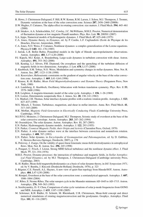
The Solar Dynamo 615

R. Howe, J. Christensen-Dalsgaard, F. Hill, R.W. Komm, R.M. Larsen, J. Schou, M.J. Thompson, J. Toomre,Dynamic variations at the base of the solar convection zone. Science 287, 2456–2460 (2000b)

D.W. Hughes, F. Cattaneo, The alpha-effect in rotating convection: size matters. J. Fluid Mech. 594, 445–461(2008)

A.B. Iskakov, A.A. Schekochihin, S.C. Cowley, J.C. McWilliams, M.R.E. Proctor, Numerical demonstrationof fluctuation dynamo at low magnetic Prandtl numbers. Phys. Rev. Lett. 98, 208501 (2007)

S.A. Jepps, Numerical models of hydromagnetic dynamos. J. Fluid Mech. 67, 625–646 (1975)C.A. Jones, Dynamo theory, in Dynamos, ed. by P. Cardin, L.F. Cugliandiolo (Ecole de Physique de les

Houches, Elsevier, Amsterdam, 2008)C.A. Jones, N.O. Weiss, F. Cattaneo, Nonlinear dynamos: a complex generalization of the Lorenz equations.

Physica D 14D, 161–176 (1985)J. Jurcak, L.R. Bellot Rubio, Penumbral models in the light of Hinode spectropolarimetric observations.

Astron. Astrophys. 481, L17–L20 (2008)P.J. Käpylä, M.J. Korpi, A. Brandenburg, Large-scale dynamos in turbulent convection with shear. Astron.

Astrophys. 491, 353–362 (2008)S.R. Keating, L.J. Silvers, P.H. Diamond, On crossphase and the quenching of the turbulent diffusion of

magnetic fields in two dimensions. Astrophys. J. Lett. 678, L137 (2008)E. Knobloch, S.M. Tobias, N.O. Weiss, Modulation and symmetry changes in stellar dynamos. Mon. Not. R.

Astron. Soc. 297, 1123–1138 (1998)A.G. Kosovichev, Helioseismic constraints on the gradient of angular velocity at the base of the solar convec-

tion zone. Astrophys. J. 469, L61–L64 (1996)F. Krause, K.-H. Rädler, Mean Field Magnetohydrodynamics and Dynamo Theory (Pergamon Press, New

York, 1980)A.S. Landsberg, E. Knobloch, Oscillatory bifurcation with broken translation symmetry. Phys. Rev. E 53,

3579–3600 (1996)R.B. Leighton, A magneto-kinematic model of the solar cycle. Astrophys. J. 156, 1–26 (1969)E.N. Lorenz, Deterministic nonperiodic flow. J. Atmos. Sci. 20, 130–141 (1963)J.A. Markiel, J.H. Thomas, Solar interface dynamo profiles with a realistic rotation profile. Astrophys. J. 523,

827–837 (1999)M.S. Miesch, J. Toomre, Turbulence, magnetism, and shear in stellar interiors. Annu. Rev. Fluid Mech. 41,

317–345 (2009)H.K. Moffatt, Magnetic Field Generation in Electrically Conducting Fluids (Cambridge University Press,

Cambridge, 1978)M.J.P.F.G. Monteiro, J. Christensen-Dalsgaard, M.J. Thompson, Seismic study of overshoot at the base of the

solar convective envelope. Astron. Astrophys. 283, 247–262 (1994)M. Ossendrijver, The solar dynamo. Astron. Astrophys. Rev. 11, 287 (2003)E.N. Parker, Hydromagnetic dynamo models. Astrophys. J. 122, 293 (1955)E.N. Parker, Cosmical Magnetic Fields, their Origin and Activity (Clarendon Press, Oxford, 1979)E.N. Parker, A solar dynamo surface wave at the interface between convection and nonuniform rotation.

Astrophys. J. 408, 707 (1993)E.N. Parker, Solar dynamo, in Encyclopedia of Geomagnetism and Paleomagnetism, ed. by D. Gubbins,

E. Herrero-Bervera (Springer, Dordrecht, 2007), p. 178K. Petrovay, J. Zsargo, On the validity of quasi-linear kinematic mean-field electrodynamics in astrophysical

flows. Mon. Not. R. Astron. Soc. 296, 245 (1998)A. Pouquet, U. Frisch, J. Léorat, Strong MHD helical turbulence and the nonlinear dynamo effect. J. Fluid

Mech. 77, 321–354 (1976)M.R.E. Proctor, Dynamo processes: the interaction of turbulence and magnetic fields, in Stellar Astrophys-

ical Fluid Dynamics, ed. by M.J. Thompson, J. Christensen-Dalsgaard (Cambridge university Press,Cambridge, 2003)

K.-H. Rädler, Mean-field magnetohydrodynamics as a basis of solar dynamo theory, in IAU Symposium 1971,ed. by V. Bumba, J. Kleczek (Dordrecht-Holland, Dordrecht, 1976), p. 323

S. Régnier, C.E. Parnell, A.L. Haynes, A new view of quiet-Sun topology from Hinode/SOT. Astron. Astro-phys. 484, L47–L50 (2008)

M. Rempel, Overshoot at the base of the solar convection zone: a semianalytical approach. Astrophys. J. 607,1046–1064 (2004)

J.C. Ribes, E. Nesme-Ribes, The solar sunspot cycle in the Maunder minimum AD-1645 to AD-1715. Astron.Astrophys. 276, 549–563 (1993)

A. Serebryanskiy, D.-Y. Chou, Comparison of solar cycle variations of solar p-mode frequencies from GONGand MDI. Astrophys. J. 633, 1187–1190 (2005)

M. Schrinner, K.H. Rädler, D. Schmitt, M. Rheinhardt, U.R. Christensen, Mean-field concept and directnumerical simulations of rotating magnetoconvection and the geodynamo. Geophys. Astrophys. FluidDyn. 101, 81–116 (2007)

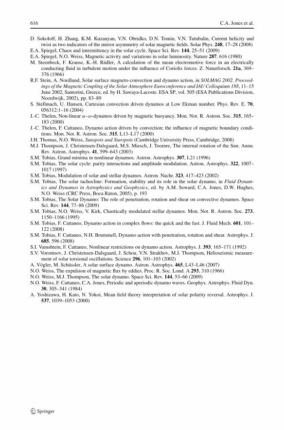
616 C.A. Jones et al.

D. Sokoloff, H. Zhang, K.M. Kuzanyan, V.N. Obridko, D.N. Tomin, V.N. Tutubalin, Current helicity andtwist as two indicators of the mirror asymmetry of solar magnetic fields. Solar Phys. 248, 17–28 (2008)

E.A. Spiegel, Chaos and intermittency in the solar cycle. Space Sci. Rev. 144, 25–51 (2009)E.A. Spiegel, N.O. Weiss, Magnetic activity and variations in solar luminosity. Nature 287, 616 (1980)M. Steenbeck, F. Krause, K.-H. Rädler, A calculation of the mean electromotive force in an electrically

conducting fluid in turbulent motion under the influence of Coriolis forces. Z. Naturforsch. 21a, 369–376 (1966)

R.F. Stein, A. Nordlund, Solar surface magneto-convection and dynamo action, in SOLMAG 2002. Proceed-ings of the Magnetic Coupling of the Solar Atmosphere Euroconference and IAU Colloquium 188, 11–15June 2002, Santorini, Greece, ed. by H. Sawaya-Lacoste. ESA SP, vol. 505 (ESA Publications Division,Noordwijk, 2002), pp. 83–89

S. Stellmach, U. Hansen, Cartesian convection driven dynamos at Low Ekman number. Phys. Rev. E. 70,056312:1–16 (2004)

J.-C. Thelen, Non-linear α–ω-dynamos driven by magnetic buoyancy. Mon. Not. R. Astron. Soc. 315, 165–183 (2000)

J.-C. Thelen, F. Cattaneo, Dynamo action driven by convection; the influence of magnetic boundary condi-tions. Mon. Not. R. Astron. Soc. 315, L13–L17 (2000)

J.H. Thomas, N.O. Weiss, Sunspots and Starspots (Cambridge University Press, Cambridge, 2008)M.J. Thompson, J. Christensen-Dalsgaard, M.S. Miesch, J. Toomre, The internal rotation of the Sun. Annu.

Rev. Astron. Astrophys. 41, 599–643 (2003)S.M. Tobias, Grand minima in nonlinear dynamos. Astron. Astrophys. 307, L21 (1996)S.M. Tobias, The solar cycle: parity interactions and amplitude modulation. Astron. Astrophys. 322, 1007–

1017 (1997)S.M. Tobias, Modulation of solar and stellar dynamos. Astron. Nachr. 323, 417–423 (2002)S.M. Tobias, The solar tachocline: Formation, stability and its role in the solar dynamo, in Fluid Dynam-

ics and Dynamos in Astrophysics and Geophysics, ed. by A.M. Soward, C.A. Jones, D.W. Hughes,N.O. Weiss (CRC Press, Boca Raton, 2005), p. 193

S.M. Tobias, The Solar Dynamo: The role of penetration, rotation and shear on convective dynamos. SpaceSci. Rev. 144, 77–86 (2009)

S.M. Tobias, N.O. Weiss, V. Kirk, Chaotically modulated stellar dynamos. Mon. Not. R. Astron. Soc. 273,1150–1166 (1995)

S.M. Tobias, F. Cattaneo, Dynamo action in complex flows: the quick and the fast. J. Fluid Mech. 601, 101–122 (2008)

S.M. Tobias, F. Cattaneo, N.H. Brummell, Dynamo action with penetration, rotation and shear. Astrophys. J.685, 596 (2008)

S.I. Vainshtein, F. Cattaneo, Nonlinear restrictions on dynamo action. Astrophys. J. 393, 165–171 (1992)S.V. Vorontsov, J. Christensen-Dalsgaard, J. Schou, V.N. Strakhov, M.J. Thompson, Helioseismic measure-

ment of solar torsional oscillations. Science 296, 101–103 (2002)A. Vögler, M. Schüssler, A solar surface dynamo. Astron. Astrophys. 465, L43–L46 (2007)N.O. Weiss, The expulsion of magnetic flux by eddies. Proc. R. Soc. Lond. A 293, 310 (1966)N.O. Weiss, M.J. Thompson, The solar dynamo. Space Sci. Rev. 144, 53–66 (2009)N.O. Weiss, F. Cattaneo, C.A. Jones, Periodic and aperiodic dynamo waves. Geophys. Astrophys. Fluid Dyn.

30, 305–341 (1984)A. Yoshizawa, H. Kato, N. Yokoi, Mean field theory interpretation of solar polarity reversal. Astrophys. J.

537, 1039–1053 (2000)