


Languages
Pages
Legal


THE RELATIONSHIP BETWEEN STOCK MARKET AND THE MACROECONOMY: EVIDENCE
FROM BOTSWANA
Programme: Master of Management in Finance and Investments
Student name: Tebogo Rapaeye Student ID: 1518338
Supervisor: Prof. Paul Alagidede

Contents
1.0 ACKNOWLEDGEMENT ............................................................................................................................ 1
2.0 ABSTRACT .............................................................................................................................................. 2
3.0 INTRODUCTION ...................................................................................................................................... 4
4.0 OBJECTIVES ............................................................................................................................................ 9
5.0 SIGNIFICANCE OF STUDY ........................................................................................................................ 9
6.0 BACKGROUND ...................................................................................................................................... 11
7.0 LITERATURE REVIEW. ........................................................................................................................... 12
8.0 DATA .................................................................................................................................................... 21
9.0 METHODOLOGY ................................................................................................................................... 23
9.1 Baseline Model ................................................................................................................................. 23
9.2 Testing long -run relationship ........................................................................................................... 24
9.3 Testing for Volatility spill overs ......................................................................................................... 25
10.0 RESULTS ............................................................................................................................................... 27
TABLE 1: STATIONARITY TESTS ..................................................................................................................... 27
TABLE 2: DESCRIPTIVE STATISTICS ................................................................................................................ 29
TABLE 3: CORRELATION RESULTS ................................................................................................................. 30
TABLE 4: OLS REGRESSION RESULTS ............................................................................................................. 31
TABLE 8: MODEL SELECTION ........................................................................................................................ 34
TABLE 9: Estimation Results of ARMA (p,q)-GARCH(p,q) Models ........................................................... 37
11.0 DISCUSSION ......................................................................................................................................... 39
12.0 CONCLUSION ....................................................................................................................................... 44
13.0 REFERENCES ......................................................................................................................................... 46
14.0 APPENDICES ............................................................................................................................................. 53

1 | P a g e
1.0 ACKNOWLEDGEMENT
I would like to express my sincere gratitude to my supervisor Professor Paul Alagidede
and his team for the collaborative work that led to the successful completion of this thesis.
Their guidance, support, insight and high standards did not only help me write a better
paper but they were a life changing experience too. I am a different and better person
because of them.
I would like to extend same to the Wits Business School team in general for always
providing a helping hand in times of need. The team was ever ready to serve, in many
instances went an extra mile to ensure that I got assistance as often as required.
2 | P a g e
2.0 ABSTRACT
This study investigates the relationship between macroeconomy and stock market. The
specific objectives are to: (a) find out the macroeconomic determinant of stock returns,
(b) establish long term relationship of macroeconomic and (c) find out if there are
volatility spill overs between macroeconomic volatilities and stock returns volatility.
Domestic Company Index (DCI) is used to represent stock returns and (a) Consumer Price
Index to represent inflation, (b) USD/BWP as exchange rates, (c) Bank rates as interest
rates and (d) M2 to represent money supply as macroeconomic variables. The relevance
of Gross Domestic Product (GDP) is highly acknowledged but due to limited data, it was
excluded from the study.
The study used monthly data of the said variables from January 1994 to December 2014
to investigate the relationship. Classic Linear Regression model is applied to establish the
explanatory power of macroeconomic variables on stock returns. Auto-Regressive
Distributed Lag (ARDL) is used to find out the long term relationship and lastly GARCH
(1,1) is applied to find out if there is volatility spill overs between macroeconomic
volatilities and stock returns volatilities.
This research established that exchange rates have a negative relationship with stock
returns and money supply has a positive relationship with stock returns. It was also noted

3 | P a g e
that there is no long term relationship between macroeconomic variables and stock
returns. Lastly, it was noted that inflation volatility and money supply volatility have a spill
over effect on stock returns volatility.
Keywords: macroeconomic variables, stock returns, volatility.

4 | P a g e
3.0 INTRODUCTION
Modern financial theory has brought a lot of insight on the relationship of risk and return.
It asserts that there is a risk that the market is willing to compensate for and the one that
is not compensated by the market (Bora and Adhikary, 2015). This theory stems from the
work of Markowitz (1952), who developed the basic portfolio theory and described
linearity between risk and return (Pamane and Vikpossi, 2014). Markowitz’s work has
triggered a lot of research around the subject. Researches are usually in two folds: some
researches are interested in establishing if indeed the relationship between risk and
return are linear, whereas others want to establish what risk is, what composite the risk,
which risk is compensated by the market and which one is not.
Empirical evidence shows that indeed there is a relationship between risk and return.
Chiang and Doong, 1999 and Garza-Gomez and Kunimura, 2000 argue that the
relationship between risk and return is linear. However, there is limited literature that
speaks of the contrary. In another dimension, risk is defined as the uncertainty of the
future outcomes (Bora and Adhikary, 2015). Portfolio theory states that there are two
types of risk: systematic risk and unsystematic (idiosyncratic) risk. Systematic risk is due
to market factors whereas unsystematic risk is caused by circumstance peculiar to the
company. Systematic risk will always remain but unsystematic risk can be eliminated

5 | P a g e
through portfolio diversification (Bora and Adhikary, 2015). Since systematic risk cannot
be eliminated, investors are always requiring compensation for bearing it.
Macroeconomic activities are known to directly impact asset prices since firms’ cash flow
and risk-adjusted discount rates change with economic conditions (Ya-Wen, 2017). Chen
et al (1986), and, Bora and Adhikary (2015) argue that systematic risk comprises
macroeconomic variables. Modigliani and Pogue, 1973; Guo and Whitelaw, 2003 argue
that there is a linear relationship between systematic risk and expected return. If these
arguments hold, then macroeconomic variables must have explanatory power on stock
returns. Macroeconomic variables have explanatory power on stock returns (Liu and
Shrestha, 2008).
Not only do macroeconomic variables have been found to have explanatory power on
stock returns but their volatilities have also been found to impact stock market volatility
(Morelli, 2002).
Findings from different studies had shown that the impact of the macroeconomic
variables on stock returns and its volatilities on stock returns volatility vary from country
to country and region to region. In certain jurisdictions a variable can have a significant
relationship with stock return but in other jurisdictions the same variable will not. It is
also discernible from literature that nature of relationship differs as well, some
6 | P a g e
relationships are positive whereas others are negative As an illustration, Alagidede and
Panagiotidis (2012) found that a positive relationship exists between stock returns and
inflation for G7 countries but Gathu et al (2015) found a negative relationship between
inflation and stock returns in Kenya . Abugri (2008) found that the high volatility of
macroeconomic variables of emerging market have resulted in stock returns of that
region being highly volatile when contrasted with stock returns volatility of developed
world, which happen to have low macroeconomic volatility.
The dissonance in the research findings about the subject matter brings to mind a
question of ‘what does finance theory say?’ There are two finance theories that have
largely been used by researchers in this area: The Arbitrage Pricing Theory (Ross, 1976)
and Discount Cash flow model/ Present Value Model. Arbitrage Pricing Theory says that
the asset returns are explained by multiple factors risk factors. Researchers like Fama,
1981, 1990; Fama and French, 1989; Schwert, 1990 and Ferson and Harvey, 1991 have
used this theory to link macroeconomic variables as risk factors and as having explanatory
power on stock returns. Discount Cash flow model relates the stock price to future
expected cash flows and the future discount rate of these cash flows. Arguing that all
macroeconomic factors that influence future expected cash flows or the discount rate by
which these cash flows are discounted should impact stock price (Humpe and Macmillian,
2007).

7 | P a g e
All being posited, the critical question is what is Botswana’s case? How is the relationship
of macroeconomic variables and stock returns like? The issue of finding macroeconomic
determinants of stock returns is of great relevance to investors’ decisions making
because, the former forms part of systematic risk, as argued by Bora and Adhikary (2015).
Sikalao-Lekobane and Lekobane (2014) used Johansen’s co-integration technique to test
the long term relationship of Botswana stock prices and selected macro-economic
variables using quarterly data for the period 1998-2012. They found that macroeconomic
variables are co-integrated with stock prices. However, this is not enough; there are still
pertinent questions that are not answered. The questions relating to volatility
transmission between macroeconomy and stock market. These questions include what
the intention of this research will establish, which is the relationship between
macroeconomic factors and stock returns in Botswana. Specifically the paper aims to
address the following questions:
1. What are the macroeconomic determinant of stock returns in Botswana?
2. Is there a long run relationship between the Botswana stock markets and its
macroeconomic determinants?
3. Are there any volatility spill overs between macroeconomic variables and stock
market?

8 | P a g e
Finding answers for the above questions is very important especially given the fact that
investors are risk-averse. Overall, the findings of this research will help settle the issue of
whether the Botswana stock market compensates its investors for systematic risk.

9 | P a g e
4.0 OBJECTIVES
In line with the research questions, the main objective of this study is to find out the
macroeconomic variables that have explanatory power on the Botswana stock returns.
The specific objectives are:
1. To identify the macroeconomic determinant of stock returns in Botswana.
2. To investigate the long run relationship between the Botswana stock market and
its macroeconomic determinants.
3. To investigate if there are any volatility spill over between macroeconomic
variables and stock returns
5.0 SIGNIFICANCE OF STUDY
The relationship of macroeconomic variables and the stock informs the Investment
Strategy. It gives a clear picture about the nature of the risk and return relationship.
Depending on the nature of the relationship, portfolio managers can decide on whether
to apply market timing strategy or buy and hold strategy, when and what to hedge e.g. a
short term relationship of macroeconomic variables and the stock returns will make a
market timing strategies more profitable than a buy and hold strategy (Shen, 2003). It is
crucial to spell out how markets are linked over time to develop an effective hedging

10 | P a g e
strategy (Walid et al, 2011). This study will therefore provide insight to investors and
portfolio managers on the dynamics between Botswana macroeconomic variables and
stock returns. Lack of knowledge about the individual country’s fundamentals may lead
to investors treating these market as if they belong to a class and fail to take advantage
of existing arbitrage opportunities (Aitken,1996; Abugri, 2008).
Additionally, the study will serve as a baseline for future research purposes by interested
authorities. It can be expounded by other scholars to determine the predictive power of
macroeconomic variables to stock market movements.
Furthermore, it will inform the policymakers on the volatility transmission between the
macroeconomy and stock exchange, a factor very critical when assessing financial market
stability. Macroeconomic volatilities have in the last decade played a major role in causing
financial crises in Mexico and Argentina (Abugri, 2008).

11 | P a g e
6.0 BACKGROUND
Botswana Share Market was established in 1989 and became the Botswana Stock
Exchange (BSE) in 1995 through the act of Parliament of Botswana (Morton et al, 2008).
It is the sixth largest stock exchange in Africa in terms of market capitalisation (Africa
strictly report, 2013). BSE is one of the representatives of an emerging market in terms of
market capitalisation, trade volume and number of listed companies (Mollah, 2006). Its
average weekly trading volume is 4,900,000 (African business central, 2014).
There are about 35 market listings and 3 stock listings indices: the Domestic Company
Index (BSE DCI); the Foreign Company Index, incorporating companies which are dual
listed on the BSE and another stock exchange; and the All Company Index, which is the
weighted average of the DCI and FCI (BSE,2014). BSE has an equity market capitalization
of P418 156.7m and debt market capitalization of P10.1bn, with private investors
estimated to account for fewer than 10% of the total market capitalization and foreign
based mining companies accounting for over 90% (BSE, 2014).

12 | P a g e
7.0 LITERATURE REVIEW.
The essence of an empirical research is to establish facts against a particular theory
and/or model. As previously highlighted, the most used finance theories to establish the
relationship of macroeconomic variables and stock returns are Arbitrage Pricing Theory
(APT) and Discount Cash Flow or Present Value Model (PVM). APT is mainly used to test
the short run relationship of macroeconomic variables and stock returns on first
difference and assuming stationarity whereas PVM has the ability to establish a long run
relationship of macroeconomic variables and stock returns (Humpe and Macmillian,
2007). On this basis, the latter is most preferred theory and it has been identified as the
appropriate theory for this study.
PVM asserts that the stock prices are determined by the expected cash flows and the
future discount rate of these cash flows. It further argues that these cash flows and
discount rates are affected by macroeconomic variables therefore a change in the
variables should influence stock prices.
The relationship between macroeconomic variables and stock returns has been
investigated from different strands; scholars such as Fama (1981) and Ritter (2004) just
investigated if the macroeconomic variables have explanatory power on stock returns.
Whereas Chen (1991), Serfing and Milijkovic (2011) investigated if the macroeconomic

13 | P a g e
variables have predictive power on stock returns or stock returns do have predictive
power on macroeconomic variables. Literature also show that certain scholars were
interested in finding out shocks and volatility transmission between the macro economy
and stock markets. These studies were conducted in different regions, using different
econometric models and data of varying time horizons.
The commonly used macroeconomic variables are: interest rate spreads, money market
rates, unemployment rates, production output and the exchange rates. In investigating
the long term relationship of stock returns, inflation and industrial production, Fama
(1981) concluded that the relationship of inflation and stock returns is negative whereas
that of industrial production and stock returns is positive. Ritter (2004) used data from
1900-2002 to analyse the relationship between economic growth and equity returns for
16 countries that represented 90% of the world market capitalisation in 1900. He found
that there is a negative correlation between per capita income growth and real equity
returns. Dimson et al (2002) established that the long term relationship between
geometric mean annual stocks is negatively correlated with arithmetic mean real per
capita annual growth
Gay (2008) applied ARIMA model to test significance of stock market returns to macro-
economic variables for four emerging market countries (Brazil, Russia, India and China).
14 | P a g e
The researcher noticed that the relationship is significance except in exchange rate and
oil prices. It was also found that there is no significance of past and present stock returns.
This suggests weak form of market efficiency. Murkherjee and Naka (1995) used the
Johansen con-integration test in the Vector Error Correction Model to test co-integration
of Japanese Stock Market prices to macroeconomic variables. They found that the stock
market is co-integrated to exchange rate, money supply, inflation rate and industrial
production, long term bond rate and short term call money rate.
Closer to Botswana , Gathu et al (2015), investigated the effects of macroeconomic
environment on stock market returns of firms in the Agricultural sector in Kenya and,
found that, exchange rate has a positive influence on the stock market returns whereas
inflation has a negative effect. In Botswana, Sikalao-Lekobane and Lekobane (2014), used
Johansen’s co-integration technique to test the long term relationship of Botswana stock
prices and selected macro-economic variables using quarterly data for the period 1998-
2012.
Still on investigating the long term relationship of macroeconomy and stock market,
some researchers have narrowed their studies to investigating a long term relationship of
a particular macroeconomic variable with stock returns. Lin (2012) studied the
comovement between exchange rates and stock prices in the Asian emerging markets.

15 | P a g e
The results suggested that the comovement between exchange rates and stock prices
becomes stronger during crisis periods, consistent with contagion or spill over between
asset prices, when compared with tranquil periods.
Gertler and Gilchrist (1994) argue that increasing interest rates (monetary tightening)
negatively affects cash flow, this affect the firms’ balance sheet and ultimately reduce the
borrowing power of the firm. The impact is even more on small firms than on large firms
because the former do not have enough collateral as opposed to the latter.
Wade and May (2005) decided to study both the short term and long term relationship of
GDP growth and equity returns. They concluded that GDP growth and equity returns have
a stable short term relationship but the relationship is unstable in the long term.
Researchers interested in investigating short term relationship only also came up with
informative findings. Alagidede and Panagiotidis (2012) studied the short term
relationship of inflation and stock returns for G7 countries using quantile regression
framework. They found out that a positive relationship existed in most cases especially
when moving to higher quantiles for the dependent variable the response increased as
well. A conclusion that informs the portfolio managers that, stocks for G7 countries can
act as an inflation hedge.

16 | P a g e
Jung and Kim (2016) used a definition of broad money M2 from Bank of Korea to
breakdown aggregate money into an underlying and non-underlying part. According to
the bank, underlying is the money held by households and non-financial corporations
sectors necessary for basic purposes such as consumptions and normal business
operations. Non-underlying is part of the money held by financial corporations and
beneficiary certificates, this money was found to directly affect macro-liquidity which
ultimately affect stock returns. In a nutshell, researchers state that unexpected changes
in money growth can cause unfavourable shifts in the investment opportunities set.
As previously specified, another strand of research is on finding out the predictive power
of either macroeconomic variables on stock returns or stock returns on macroeconomic
variables. Chen (1991) states that lagged production growth rate, the default premium,
term premium, short –term interest rate and the market dividend price ratio are
indicators of recent and future economic growth.
Serfing and Milijkovic (2011) in their time series analysis of the relationships among
(macro) economic variables , the dividend yield and the price level of the S&P 500 index,
concluded that previous changes in the dividend yield ,interest rates, the money supply
and the CPI predict current changes in the dividend yield. Furthermore, that previous
changes in the dividend yield, interest rates, the S&P 500, the money supply the Industry

17 | P a g e
Production Index (IPI) and the CPI predict current changes in the yield on the 10 year
Treasury note. They used the Vector Error Correction Model (VECM) to analyse monthly
data from January 1959 to December 2009.
Gupta and Modise (2013) examined the predictability of South Africa stock returns using
macroeconomic variables. Their analysis was based on a predictive regression framework,
using monthly data covering the in-sample period between 1990:01 and 1996:12, and the
out-of sample period commencing from 1997:01 to 2010:06. The in-sample revealed that
different interest rate variables, world oil production growth and money supply have
some predictive power at certain short-horizons. The out-of-sample showed that interest
rates and money supply have short-horizon predictability. Inflation rate revealed a very
strong out-of-sample predictive power from 6-month-ahead horizons.
In the shocks and volatility transmission stream, other eye opening findings were noted.
Zhao (2010) investigated the case of China by analysing the dynamic relationship between
Renminbi (RMB) real effective exchange rate and stock price using VAR and multivariate
Generalized Autoregressive Conditional Heteroskedasticity (GARCH) models using
monthly data from January 1991 to June 2009.The findings of the study were that there
were no mean spillovers between the foreign exchange and stock markets. But there
18 | P a g e
were bidirectional volatility spillovers effects between the Foreign Exchange market and
Stock Market.
Walid et al (2011) employed a Markov-Switching EGARCH model to investigate the
dynamic linkage between stock price volatility and exchange rate changes for four
emerging countries (Hong Kong, Singapore, Malaysia and Mexico) over the period 1994–
2009. The exercise was in two regimes: conditional mean which is high mean –low
variance and the conditional variance of stock returns which is low mean and a high
variance. The results provided strong evidence that the relationship between stock and
foreign exchange markets is regime dependent and stock price volatility responds
asymmetrically to events in the foreign exchange market. An indication that foreign
exchange rate changes have a significant impact on the probability of transition across
regimes.
Tsai (2015) investigated how the United States (U.S.) stock returns responded to oil price
shocks during the pre-crisis, within the financial crisis, and post-crisis by a long time series
of daily data for 682 firms over a period of 12 years from January, 1990 to December,
2012. The results showed that U.S. stock returns responded positively to the changes in
oil prices during and after such a crisis.

19 | P a g e
Generally, literature demonstrates that macroeconomic variables have explanatory
power on the stock returns and vice versa. There is volatility and shock transmission
between macroeconomic variables and stock market. It is worth noting that mostly, the
extant literature focuses on the developed economies thereby creating a huge knowledge
gap on the case of Africa despite it being an emerging market. Limited research in African
space does not only disadvantage resident portfolio managers in crafting appropriate
investment strategy but it also denies international investors a platform for broader
portfolio diversification.
Even though it is acknowledged that Sikalao –Lekobane and Lekobane investigated the
relationship of Botswana macroeconomy and stock returns but their study is only limited
to the long term relationship without addressing volatility spillovers.
They used a small sample, quarterly data from 1998-2012. A small sample provides
unreliable results. Verial (2010) argues that a small sample has a low statistical power. A
statistical power is the ability of a statistical test based on a sample to show traits that
truly exist on the population. He also argues that a small sample fails to detect significant
details. This research will use monthly data from 1994-2014 a relatively large sample
size.

20 | P a g e
Sikao –Lekobane and Lekobane (2014), used Johansen co-integration technique but our
proposed methodology is AutoRegressive Distributed Lag (ARDL). The latter is more
thorough and detailed than the former. ARDL is more robust for co-intergration analysis
with small sample study (Pesaran et al, 2001). One of the advantages of using ARDL is
that it is applicable regardless of the stationary properties or irrespective of whether the
regressors are purely I(0) or I(1), or mutually integrated (Adu and Marbuah,2011). A
better econometric model means results that are more reliable. The present study will
therefore be a gap filler in this space.

21 | P a g e
8.0 DATA
There is no particular theory that spells out macroeconomic variables which are expected
to have explanatory power on stock returns. Therefore objectivity in the selection of
variables is always questionable. This is an unavoidable problem associated with this area
of research (Fama, 1991). Researchers usually resort to using previous studies as a guide
and this research intends to do the same. Chen et al. (1986), Murkherjee and Naka (1995)
and Gathu et al. (2015) had used inflation, Gross Domestic Product, Interest and
exchanges rates to test their explanatory power on stock returns.
The researcher intends to use Consumer Price Index as a proxy for inflation. USD/BWP
exchange rate because the US Dollar is largely used in Botswana for international trade.
Bank Rates as a proxy for interest rates and lastly M2 to proxy money supply. Gross
Domestic Product is not included because of lack of its data for the desired period but its
relevance is highly acknowledged. The Domestic Company Index (DCI) will be used to
proxy the local stock. The researcher intends to use monthly data spanning from January
1994 to December 2014. Data on Macroeconomic variables was solicited from Bank of
Botswana and data on Domestic Company Index is from Botswana Stock Exchange.
The researcher will use the returns for DCI because of their stationarity property over
prices and they will be calculated as:
𝑅𝑡 = ln(𝑃𝑡 ) − ln 𝑃𝑡−1 (1)
Where Rt is the stock market return in month t, ln is the logarithm, and Pt is the DCI at
the end of month t. Stationarity for stock returns will be tested using the Augmented
Dickey-Fuller test.

22 | P a g e
The first differences in the log of macroeconomic variables will be taken. This is meant to
ensure stationarity of the macroeconomic variables. The same Augmented Dickey-Fuller
test will be conducted to also test for stationarity of the regressors. The data will also be
tested for normality, skewness and Kurtosis (descriptive statistics).
23 | P a g e
9.0 METHODOLOGY
9.1 Baseline Model
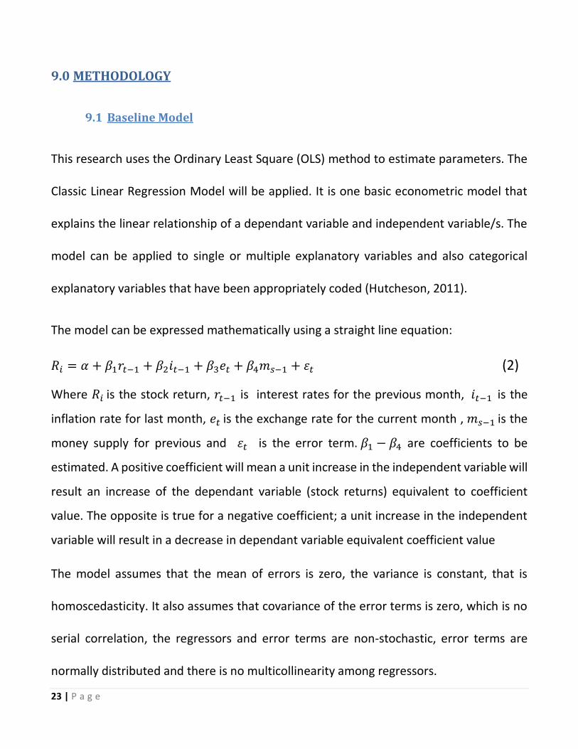
This research uses the Ordinary Least Square (OLS) method to estimate parameters. The
Classic Linear Regression Model will be applied. It is one basic econometric model that
explains the linear relationship of a dependant variable and independent variable/s. The
model can be applied to single or multiple explanatory variables and also categorical
explanatory variables that have been appropriately coded (Hutcheson, 2011).
The model can be expressed mathematically using a straight line equation:
𝑅𝑖 = 𝛼 + 𝛽1𝑟𝑡−1 + 𝛽2𝑖𝑡−1 + 𝛽3𝑒𝑡 + 𝛽4𝑚𝑠−1 + 𝜀𝑡 (2)
Where 𝑅𝑖 is the stock return, 𝑟𝑡−1 is interest rates for the previous month, 𝑖𝑡−1 is the
inflation rate for last month, 𝑒𝑡 is the exchange rate for the current month , 𝑚𝑠−1 is the
money supply for previous and 𝜀𝑡 is the error term. 𝛽1 − 𝛽4 are coefficients to be
estimated. A positive coefficient will mean a unit increase in the independent variable will
result an increase of the dependant variable (stock returns) equivalent to coefficient
value. The opposite is true for a negative coefficient; a unit increase in the independent
variable will result in a decrease in dependant variable equivalent coefficient value
The model assumes that the mean of errors is zero, the variance is constant, that is
homoscedasticity. It also assumes that covariance of the error terms is zero, which is no
serial correlation, the regressors and error terms are non-stochastic, error terms are
normally distributed and there is no multicollinearity among regressors.

24 | P a g e
The effect of unexpected economic news on stock prices is sometimes lagged because of
the delay in the transmission and incorporation of information. Exchange rates are the
only variables that have been seen to have an instantaneous effect because they are
published every day (Bilson et al, 2001). The lagged effect of the variables will also be
tested except exchange rates which will be tested for both instantaneous and lagged
effect.
9.2 Testing long -run relationship
The co-integration method by Pesaran et al (2001) called Autoregressive –Distributed Lag
(ARDL) will be applied. One of the advantages of using ARDL is that, it is applicable
regardless of the stationary properties or irrespective of whether the regressors are
purely I(0) or I(1), or mutually integrated (Adu and Marbuah, 2011). Moreover, the
bounds test approach is robust for co-integration analyses with small sample study
(Pesaran et al, 2001). With respect to equation (3), the ARDL framework for stock returns
model is:
∆𝑅=а + ∑ 𝑏𝑚𝑖=0 ∆rt-1+ ∑ 𝑏𝑚
𝑖=0 ∆it-1+ ∑ 𝑏𝑚𝑖=0 ∆et+ ∑ 𝑏𝑚
𝑖=0 ∆ms-1 +λ0rt-1 + λ1𝑖t-1 +λ 2et +λ 3ms-1 +
Ɛt. (3)
Where ∆ is the difference in the operator and Ɛt is the disturbance error term assumed
to be white noise. The long run relationship between the concerned variables will be
conducted based on the Wald test (F-statistic ) by imposing the variables equal to zero,
that is H0:λ0=λ1=λ2=λ3 =0against H1: λ0≠λ1≠λ2≠λ3≠0.
Incorporating the error correction model, then the formula is:
25 | P a g e
∆𝑅= а0+ ∑ 𝑏𝑚𝑖=0 1∆rt-1 +∑ 𝑏𝑚
𝑖=0 2∆it-1 +∑ 𝑏𝑚𝑖=0 3∆e +∑ 𝑏𝑚
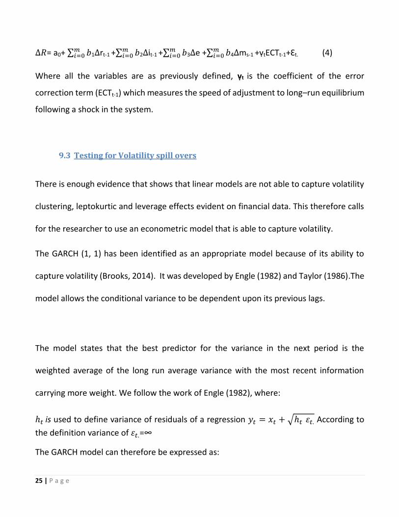
𝑖=0 4∆ms-1 +ṿtECTt-1+Ɛt. (4)
Where all the variables are as previously defined, ṿt is the coefficient of the error
correction term (ECTt-1) which measures the speed of adjustment to long–run equilibrium
following a shock in the system.
9.3 Testing for Volatility spill overs
There is enough evidence that shows that linear models are not able to capture volatility
clustering, leptokurtic and leverage effects evident on financial data. This therefore calls
for the researcher to use an econometric model that is able to capture volatility.
The GARCH (1, 1) has been identified as an appropriate model because of its ability to
capture volatility (Brooks, 2014). It was developed by Engle (1982) and Taylor (1986).The
model allows the conditional variance to be dependent upon its previous lags.
The model states that the best predictor for the variance in the next period is the
weighted average of the long run average variance with the most recent information
carrying more weight. We follow the work of Engle (1982), where:
ℎ𝑡 is used to define variance of residuals of a regression 𝑦𝑡 = 𝑥𝑡 + √ℎ𝑡 𝜀𝑡. According to
the definition variance of 𝜀𝑡.=∞
The GARCH model can therefore be expressed as:

26 | P a g e
ℎ𝑡+1 = 𝜔 + 𝛼(𝑦𝑡 − 𝑥𝑡)2 + 𝛽ℎ𝑡 = 𝜔 + 𝛼ℎ𝑡𝜀𝑡2 + 𝛽ℎ𝑡 (5)
The econometricians must estimate the constants 𝜔,𝛼, 𝛽; updating simply requires
knowing the previous forecast h and residual. The weights are (1- 𝑎- 𝛽, 𝛽, 𝑎 ) and the long
run average variance is√𝜔/(1 − 𝛼 − 𝛽. It should be noted that this is a condition for
GARCH (1, 1) if 𝛼 + 𝛽 < 1, and only really makes sense if the weights are positive
requiring 𝛼 > 0, 𝛽 > 0, 𝜔 > 0
MODEL SELECTION
Akaike Information Criterion (AIC) will be used to select a better model. The AIC statistic
is discussed below:
T
n
nTAIC
T
i
i2
ˆ
ln 1
2
(6)
Where 2ˆi is the estimated squared residuals of the model, T is the number of observations
in the sample and n is the number parameters estimated including the constant. A better
model is the one with the lowest AIC.

27 | P a g e
10.0 RESULTS
Prior to running regressions, data was tested for stationarity under the null hypothesis:
H0: θ= 0 (i.e. unit root is present) and alternative hypothesis H1: θ˂ 0 (i.e. unit is not
present). Table 1 shows ADF unit root tests results; null hypothesis is rejected under all
variables. This means data is stationary. It is appropriate to use stationary data because
the shock gradually dies away but in a non-stationary data the shocks will always be
infinite (Brooks, 2014).The author also argues that non stationary data causes spurious
regressions and violates asymptotic analysis assumption.
TABLE 1: STATIONARITY TESTS
VARIABLE CRITICAL VALUE
(5%)
ADF STATISTIC P VALUE
DCI -3.44 -8.67 <0.0001
CPI -3.43 -7.34 <0.0001
EXCHANGE RATES -3.43 -11.22 <0.0001
INTEREST RATES -3.43 -7.90 <0.0001
MONEY SUPPLY -3.43 -18.82 <0.0001
Note :< 0.0001 indicates significance at 1%
Table 2 reports the summary statistics of the variables. DCI has a positive mean which
implies that generally the stock returns have being positive over time. Standard Deviation
is highest in DCPI (8.03) meaning that inflation is highly volatile when compared with

28 | P a g e
other variables. DMS has the second largest volatility and lastly is the DCI .This could mean
that stock returns volatility is driven by inflation volatility and money supply volatility,
however this will be confirmed by the results on volatility transmission.
The skewness results indicate that DCIRET (1.39) and DMS (1.76) are positively skewed.
DCPI (-0.03), DER (-1.41) and DINTRATE (-2.56) are negatively skewed. In a normal
distribution, the mean and the median are the same but in a skewed data they are
different. A negatively skewed data will have a mean left of the median and a positively
skewed data will have mean on the right of the median. Kurtosis measures the fatness of
the tails of the data distribution and how the mean peaked is. Normally peaked mean has
a kurtosis of 3 and excess kurtosis of 0. All variables have excess kurtosis of more than 0,
which means they are leptokurtic and they have fat tails than those of a normal
distribution.
Normality is being tested using Jarque –Bera tests (Brooks, 2014). The null hypothesis
states that data is normally distributed but results prove it wrong so the null is rejected,
that is data is not normally distributed. There are no missing observations in any variable.

29 | P a g e
TABLE 2: DESCRIPTIVE STATISTICS
DCI CPI ER INT MS
MEAN 1.40 -0.44 -0.52 -0.23 1.27
MEDIAN 0.92 0.00 -0.39 0.00 0.83
STD 3.87 8.03 2.67 1.80 4.65
SKEWNESS 1.39 -0.03 -1.41 -2.56 1.76
KURTOSIS 9.38 7.06 9.43 16.47 12.80
JARQUE B 506.30 172.09 515.21 2172.53 1134.50
PROBABILITY 0.00 0.00 0.00 0.00 0.00
Note: DCI: Domestic company Index, CPI: Consumer Price Index, ER: Exchange Rate,INT: Interest rates MS; Money supply STD: Standard Deviation, Jarque Bera. Probability: 0.00 means significance at 1%
Table 3 reports correlation results. Correlation measures the relationship between
variables. Its coefficients range between -1 and +1. -1 indicates that the variables are
perfectly negatively correlated and +1 indicates that variables are perfectly positively
correlated. A negative correlation means that as one variable increases, the other
decreases whereas a positive correlation means that as one variable increases the other

30 | P a g e
one also increases. Results clearly show DCI RETURNS are weakly negatively correlated to
inflation and exchange rate with correlation coefficients of -0.45 and -0.12 respectively.
But weakly positively correlated to interest rates and money supply with correlation
coefficients of 0.039 and 0.091 respectively.
TABLE 3: CORRELATION RESULTS Correlation
Probability DCIRET DCPI DINTRATE DER DMS
DCIRET 1.000000
-----
DCPI -0.044547 1.000000
(0.4823) -----
DINTRATE 0.039220 0.144923 1.000000
(0.5362) (0.0216 ) -----
DER -0.123191 -0.065883 -0.095528 1.000000
(0.0512 ) (0.2985) (0.1312) -----
DMS 0.091135 0.037156 -0.014339 0.001912 1.000000
(0.1500) (0.5579 ) (0.8212) (0.9760 ) -----
Note: DCIRET is the DCI returns, DCPI is inflation, DER is the exchange rate , DINTRATE is the interest rate and DMS is the
money supply . Figures in ( ) are p values.
Table 4 reports OLS regression results. Exchange rate and Money supply have a significant
relationship at 10%, other variables do not have a significant relationship. A negative
coefficient for exchange rates (DER) means that as exchange rates increases by 1 unit in
the current month, DCI decreases by about 0.15 in the same month. A positive coefficient
for money supply indicates that as money supply increases by 1 unit in the previous
month, stock returns will increases by 0.06 in the current month.

31 | P a g e
TABLE 4: OLS REGRESSION RESULTS
VARIABLE COEFFICIENT STD ERROR T-STATISTIC
C 1.18*** 0.40 2.94
DCPI(-1) -0.01 0.02 -0.56
DINT(-1) -0.04 0.08 -0.15
DER -0.1* 0.08 -1.00
DER(-1) -0.08 0.08 -1.00
DMS(-1) 0.06* 0.03 1.95
AR(1) 0.71*** 0.06 11.26
AR(2) -0.20*** 0.06 -3.20
Note: DCPI (-1) is the 1 month lagged CPI, DINT (-1) is 1 month lagged interest rates, DER is the exchange rate for the current month, DER (-1) is 1 month lagged exchange rate, DMS (-1) is 1 month lagged money supply. * and *** are significance levels at 10% and 1% respectively.

32 | P a g e
In selecting the model for ARDL, the Akaike Information Criteria was used again. Results
show that ARDL (3, 0, 0, 1, 2) is best model. Table 5 reports the results.
TABLE 5: ARDL MODEL SELECTION
-4.139
-4.138
-4.137
-4.136
-4.135
-4.134
-4.133
-4.132
-4.131
-4.130
AR
DL(
3, 0
, 0,
1, 2
)
AR
DL(
3, 0
, 0,
0, 2
)
AR
DL(
4, 0
, 0,
0, 2
)
AR
DL(
3, 0
, 1,
0, 2
)
AR
DL(
4, 0
, 1,
0, 2
)
AR
DL(
3, 0
, 1,
1, 2
)
AR
DL(
4, 0
, 0,
1, 2
)
AR
DL(
3, 0
, 0,
2, 2
)
AR
DL(
4, 0
, 1,
1, 2
)
AR
DL(
3, 0
, 0,
0, 3
)
AR
DL(
3, 0
, 0,
1, 3
)
AR
DL(
4, 0
, 0,
2, 2
)
AR
DL(
3, 0
, 1,
2, 2
)
AR
DL(
3, 1
, 0,
0, 2
)
AR
DL(
4, 0
, 0,
0, 3
)
AR
DL(
4, 0
, 2,
0, 2
)
AR
DL(
3, 1
, 0,
1, 2
)
AR
DL(
4, 1
, 0,
0, 2
)
AR
DL(
3, 0
, 2,
0, 2
)
AR
DL(
3, 0
, 1,
0, 3
)
Akaike Information Criteria (top 20 models)
NOTE: a model with lowest AIC value is the best model.

33 | P a g e
As stated in the methodology, ARDL is chosen model for testing long term relationship,
results show that all the coefficients are significant. However, it should be noted that
conclusions about the results will be made on the basis of bounds test (table 7).
TABLE 7: BOUNDS TEST RESULTS
Test Statistic Value k F-statistic 2.084790 4
Critical Value Bounds Significance I0 Bound I1 Bound 10% 2.2 3.09
5% 2.56 3.49
2.5% 2.88 3.87
1% 3.29 4.37 Note: the F-statistic is lower than the lower (IO) this means there is no long run relationship between stock returns and
macroeconomic variables.

34 | P a g e
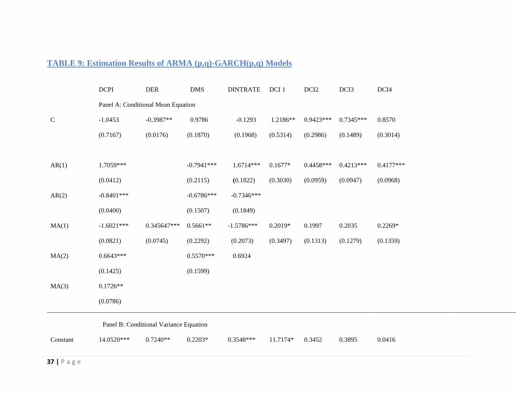
Model selection for mean models is based on Akaike Information Criteria (AIC). A model
with the lowest AIC is the most appropriate one. Table 8 shows results for best model
based on AIC amongst possible all ARMA (p,q) for each variable.
TABLE 8: MODEL SELECTION FOR MEAN MODELS
Variable ARMA(p,q) AIC
DCI (1,1) 5.08
CPI (2,3) 6.92
Exchange Rates (0,1) 4.69
Interest Rates (2,3) 3.87
Money Supply (2,3) 5.89
Note: AIC is the Akaike Information Criteria. ARMA (p,q) represents the appropriate Auto
Regressive Moving Average model.
The mean values selected as shown in table 8 were subtracted from historical values, the
difference were squared to get variance i.e. conditional volatility for each macroeconomic
variable. Heteroscedasticity was present in Lag 15 of the CPI, autocorrelation also noted
in the variables. This necessitated the use of GARCH model. We used each
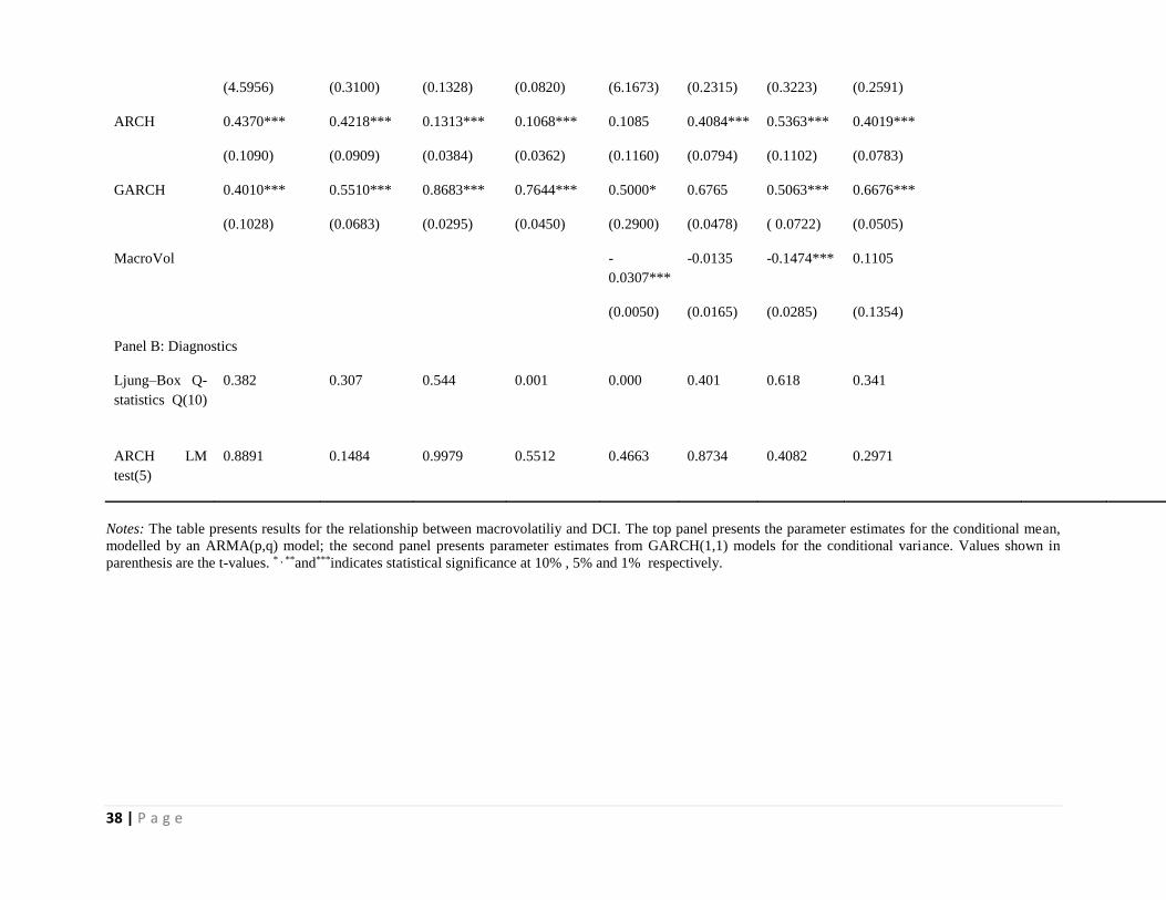
macroeconomic volatility as explanatory variable for DCI variable and the results are in
table 9. DCI1 represents regression results for CPI vol and DCI, DCI2 is the regression

35 | P a g e
results for Exchange Rate(ER) and DCI. DCI 3 is regression results for Money supply
volatility and DCI, lastly DCI4 is the results for Interest rates volatility and DCI. The results
indicate that there is volatility transmission between macroeconomy and stock returns
.They show that inflation volatility and money supply volatility drives stock returns
volatility. These findings are consistent with what descriptive statistics is showing.
Inflation, Stock returns have high standard which indicates high volatility because
volatility is standard deviation squared. Heteroscedasticity was tested after applying
GARCH and results revealed that there is no heteroscedasticity. Autocorrelation was also
tested using a correlogram and the conclusion reached was that there is no
autocorrelation (graphs in appendices).

36 | P a g e
37 | P a g e
TABLE 9: Estimation Results of ARMA (p,q)-GARCH(p,q) Models
DCPI DER DMS DINTRATE DCI 1 DCI2 DCI3 DCI4
Panel A: Conditional Mean Equation
C -1.0453 -0.3987** 0.9786 -0.1293 1.2186** 0.9423*** 0.7345*** 0.8570
(0.7167) (0.0176) (0.1870) (0.1968) (0.5314) (0.2986) (0.1489) (0.3014)
AR(1) 1.7059*** -0.7941*** 1.6714*** 0.1677* 0.4458*** 0.4213*** 0.4177***
(0.0412) (0.2115) (0.1822) (0.3030) (0.0959) (0.0947) (0.0968)
AR(2) -0.8401*** -0.6786*** -0.7346***
(0.0400) (0.1507) (0.1849)
MA(1) -1.6021*** 0.345647*** 0.5661** -1.5786*** 0.2019* 0.1997 0.2035 0.2269*
(0.0821) (0.0745) (0.2292) (0.2073) (0.3497) (0.1313) (0.1279) (0.1359)
MA(2) 0.6643*** 0.5570*** 0.6924
(0.1425) (0.1599)
MA(3) 0.1726**
(0.0786)
Panel B: Conditional Variance Equation
Constant 14.0520*** 0.7240** 0.2203* 0.3548*** 11.7174* 0.3452 0.3895 0.0416
38 | P a g e
(4.5956) (0.3100) (0.1328) (0.0820) (6.1673) (0.2315) (0.3223) (0.2591)
ARCH 0.4370*** 0.4218*** 0.1313*** 0.1068*** 0.1085 0.4084*** 0.5363*** 0.4019***
(0.1090) (0.0909) (0.0384) (0.0362) (0.1160) (0.0794) (0.1102) (0.0783)
GARCH 0.4010*** 0.5510*** 0.8683*** 0.7644*** 0.5000* 0.6765 0.5063*** 0.6676***
(0.1028) (0.0683) (0.0295) (0.0450) (0.2900) (0.0478) ( 0.0722) (0.0505)
MacroVol
-
0.0307***
-0.0135 -0.1474*** 0.1105
(0.0050) (0.0165) (0.0285) (0.1354)
Panel B: Diagnostics
Ljung–Box Q-
statistics Q(10)
0.382 0.307 0.544 0.001 0.000 0.401 0.618 0.341
ARCH LM
test(5)
0.8891 0.1484 0.9979 0.5512 0.4663 0.8734 0.4082 0.2971
Notes: The table presents results for the relationship between macrovolatiliy and DCI. The top panel presents the parameter estimates for the conditional mean,
modelled by an ARMA(p,q) model; the second panel presents parameter estimates from GARCH(1,1) models for the conditional variance. Values shown in
parenthesis are the t-values. * , **and***indicates statistical significance at 10% , 5% and 1% respectively.

39 | P a g e
11.0 DISCUSSION
The Botswana case is very peculiar; most of results are in dissonance with what
Present Value Model says. The theory asserts macroeconomic variables should
impact stock returns because of their ability to affect the expected cash flows
and discount rate. The researcher expected that all the macroeconomic
variables will have explanatory power on stock returns and also a long run
relationship between macroeconomic variables and stock returns.
The OLS regression results show that inflation does not have explanatory power
on stock returns which implies that inflation does not affect Botswana stock
returns. Theoretically, it is expected that inflation will have a significant negative
relationship with the stock returns because inflation is a component of interest
rates and interest rates are used as discount rates for fundamental stock
valuation. Most empirical studies including the likes of Fama (1981) and Gathu
et al (2015) do confirm that indeed inflation have a negative impact on the stock
returns. The findings of this study are inconsistent with both theory and most of
the literature.
International Trade and International Portfolio diversification have advanced
discussions around exchange rate to be central to economic decision making.
The issue of whether the exchange rate should have a negative or positive

40 | P a g e
impact on the stock returns is a function of the whether a country is import
oriented or export oriented. In an import based economy, strengthening of the
major trading foreign currency relative to a domestic currency will have a
negative impact of stock returns but in an export oriented economy weakening
of domestic currency relative to that of a foreign currency will have a positive
impact. Botswana is an import based economy so it is expected that
strengthening USD against BWP (domestic currency) will have a negative on
domestic stock returns. The results are consistent with expectation, they
showed that USD/BWP exchange rate have a significant negative relationship
with stock returns. The results imply that, as the USD strengthens against BWP,
the DCI returns declines. The situation calls for portfolio managers to identify a
hedging strategy against the strengthening of the USD. If BWP strengthen
against USD then DCI returns improves. All else being equal, strategic
management of USD/BWP exchange rate can be used to improve Botswana
stock returns.
Financial Economists have conflicting views when it comes to how money
supply affects stock returns. The real activists economists hold the view that a
positive shock in the money supply will increase stock prices .On the contrary,
others like Sellin (2001) hold the view that an expansionary money policy will
lead to expectation of contractionary monetary policy in the future, this will

41 | P a g e
result in increased interest rates which will ultimately result in low stock returns.
The results of this study are consistent with the views of the real activists
economists. The results show that money supply has a positive impact on stock
returns, meaning that, an expansionary monetary policy will increase stock
returns but a contractionary monetary policy will shrink DCI returns. The results
are also in agreement with the findings of Jung and Kim (2016).
Interest rates by virtue of them being a cost of borrowing, are expected to have
a negative impact on the stock returns but the findings of the study show that
they have an insignificant relationship with stock returns. These findings are
inconsistent with both theory and empirical research by Serfing and Milijkovic
(2011).
The long run relationship of the macroeconomic variables and stock returns was
tested using ARDL model. The results indicate that there is no long run
relationship that exists between the macroeconomic variables and stock
returns. These results were highly unexpected especially given that a similar
study was carried out by Sikalao-Lekobane and Lekobane (2014), who realised
that stock returns are co-integrated with macroeconomic variables. It is
acknowledged that the duo used Johansen co-integration model but still, it was
expected that the results will be the same more so that the period covered by
both researches are close. These findings imply that investors are not

42 | P a g e
compensated for bearing systematic risk for a long time. In an environment like
Botswana, a buy and hold strategy is inappropriate, portfolio managers should
rather apply market timing strategy (Shen, 2003).
The third objective of this study was to establish if there is volatility spill over
between macroeconomic volatilities and stock return volatilities. It was found
out that inflation and money supply volatilities have a spill over effects on stock
returns volatility. These results link very well with the results of the data
description where it was found that inflation and money supply have the highest
volatilities (measured by squaring standard deviation) amongst other
macroeconomic variables.
Even though it is expected that macroeconomic volatilities will drive stock
returns volatilities because previous studies like Abugri (2008) show that, this is
a cause for concern because macroeconomic volatilities increases risk premia
and hedging costs (Rother, 2004). However, investors should not be bothered
much by both inflation and money supply volatilities because Botswana has a
good Monetary Policy appropriate for managing the volatilities. Botswana
monetary policy frame work makes inflation and monetary policy interventions
very predictable (Bank of Botswana, 2016).
The results of this study justifies the essence of empirical research, they present
the evidence that theory is not always correct and also that; what is the case in

43 | P a g e
one jurisdiction is not necessarily the case in another jurisdiction. The fact that
some of the findings of this study are inconsistent with what theory says and
also what literature show does not mean they are wrong, but they rather
demonstrate the uniqueness of Botswana case. The difference between our
findings and those of Sikalao-Lekobane and Lekobane (2014) is attributable to
different econometric methods applied and also the varying sample size.

44 | P a g e
11.0 CONCLUSION
The purpose of this study is to find out the relationship of macroeconomy and
stock returns in Botswana with specific objectives of: (a) identifying the
macroeconomic determinant of stock returns in Botswana, (b) investigating the
long run relationship between the Botswana stock market and its
macroeconomic determinants and lastly investigating if there are any volatility
spill over between macroeconomic volatilities and stock returns.
The OLS model used to find out the macroeconomic determinants of stock
returns, ARDL model was used to investigate the long run relationship and
GARCH method was used to test volatility spill overs. The objectives of this study
have being met and the researchers confidently conclude by saying; money
supply and exchange rates are macroeconomic determinants of stock returns in
Botswana.
There is no long run relationship between stock returns and macroeconomy.
Inflation volatility and Money supply volatility drives stock returns volatility,
thanks to transparent monetary framework policy which makes it easy for
investors to manage volatility.
We are pleased with the significance of this study to the investors, portfolio
managers and policy makers. However, there are still certain questions that are

45 | P a g e
not answered. It is still not known how GDP affects stock returns in Botswana
and also what the relationship of the macroeconomy and stock returns under
extreme economic conditions is. Therefore it is recommended that, in future
when there is enough sample data, a study be carried out to establish the
relationship between GDP and stock returns. Once again, we recommend for a
study that will establish the relationship of macroeconomy and stock returns
under extreme economic climates which are recession and boom.

46 | P a g e
12.0 REFERENCES
Abugri,B.A.(2008).Empirical relationship between macroeconomic volatility and
stock returns: Evidence from Latin American markets. International Review of
Financial Analysis, 17,396-410.
Adu, G.,Marbuah,G.(2011).Determinants of Inflation in Ghana: An Empirical
Investigation. South African Journal of Economics, 79(3).
Aitken, B. (1996).Have institutional investors destabilized emerging markets?
Working paper, 96/34. Washington DC: International Monetary Fund.
Alagidede, P., Panagiotidis, T. (2012).Stock returns and inflation: Evidence from
quantile regressions. Economics letters, 117,283-286.
Bilson, C. M.,Brailsford, T.J., Hooper, V. J. (2001). Selecting macroeconomic
variables as explanatory factors of emerging stock market returns.Pacific-Basin
Finance Journal,9,401-426.
Bora, B., Adhikary, A. (2015). Risk and Return Relationship-An Empirical Study of
BSE Sensex Companies in India. Universal Journal of Accounting and Finance,
3(2):45-51.
Brooks, C. (2014). Introductory Econometrics for Finance (third
edition).Cambridge University Press
Chen, N. F. (1991). Financial Investments opportunities and the Macroeconomy.
The journal of Finance, 46,529-54
Chen, N. F., Ross, S. (1986). Economic Forces and the stock market. Journal of
Business, 59(3), 83-403

47 | P a g e
Cheung, Y., Ng, L.G. (1998). International Evidence on the stock market and
aggregate economic activity. Journal of Empirical Finance, (5) 281-296.
Chiang, T.C.,Doong, S.C.(1999). Emperical Analysis of realand financial
volatilities on stock returns. Global Finance Journal, 10,187-200.
DeFina, R. H., (1991). Does Inflation Depress the stock market? Federal Reserve
Bank of Philadelphia Business Review, 11(pp. 3-12).Philadelphia,Pennsylvania.
Dimson, E., Marsh,P., Stauton, M.(2002). Triumph of the Optimists: 101 Years of
Global Investments Returns. Princeton University Press. Princeton
Engle, R. (1982). Autoregressive Conditional Heteroscedasticity with Estimates
of the variance of United Kingdom Inflation. Econometrica, (50) 987-1007.
Garza-Gomez, X., Kunimura, M. (2000). Cross-Sectional Regression analysis of
return and beta in Japan. Journal of Economics and Business,52(1),515-533
Gathu, S., Gekara, M., Muturi, W. (2015). Effect of Macroeconomic Environment
on Stock Market Returns of Firms in the Agricultural Sector in Kenya. IJMBS, 5(3).
Gay, R. D. (2008). Effect of macroeconomic variables on stock market returns for
four emerging markets economies: Brazi,Russia,,India and China. International
Business and Economics Research Journal, 7(3), 1-8.
Gertler, M., Gilchrist, S. (1994). Monetary policy, business cycles, and the
behaviour of small manufacturing firms, Journal of Economics, 109,310-338
Guo, H., Whitelaw, R. F. (2003). Uncovering the Risk and Return Relation in the
stock market. Working paper series. Stern School of Business. New York
University. New York
Gupta, R., Modise, M. P. (2013). Macroeconomic Variables and South African
Stock Return Predictability. Economic Modelling, 30, 612-622.

48 | P a g e
Fama, E. (1981). Stock returns, real activity, inflation and money. American
Economic Review, 71, 545-565.
Fama, E., (1990).Stock returns, expected returns, and real activity. Journal of
Finance, 45, 1575-1617.
Fama, E F. (1991). Efficient capital markets. Journal of Finance 46, 1575-1617.
Fama, E., French, K.R., (1989), Business conditions and expected returns on
stocks and bonds. Journal of Financial Economics, 25, 23-49.
Ferson, W., Harvey, C. (1991). The variation of economic risk premiums. Journal
of Political Economy, 99, 385-415.
http://www.bankofbotswana.bw/assets/uploaded/MONETARY%20POLICY%20
S%202016%20WEBSITE%20FINAL%20NEW%20BANK%20OF%20BOTSWANA.pd
f
http://www.bse.bw/docs/BSE%20ANNUAL%20REPORT%202013.pdf
http://science.com/effects-small-sample-size-limitation-8545371.html
Humpe, A., Macmillan, P. (2007). Can macroeconomic variables explain long
term stock market movements? A comparison of the US and Japan. Working
papers series.07/20. Centre for Dynamic Macroeconomic Analysis. School of
Economics and Finance, University of St Andrews, Castlecliffe.
Hutcheson, G.D. (2011).The SAGE Dictionary of Quantitative Management
Research (pp 224-228).Sage
Jung, H., Kim, D. (2016). Macro Liquidity Risk, Money Growth, and the Cross-
Section of Stock Returns: The Case of Korea. Emerging Markets Finance &
Trade, 52, 1438-1454.
49 | P a g e
Lin, C. (2012). The comovement between exchange rates and stock prices in the
Asian emerging markets. International Review of Economics and Finance,
22,161-172.
Liu, M., Shrestha, K. M. (2008). Analysis of the long-term relationship between
macro-economic variables and the Chinese stock market using heteroscedastic
cointegration. Managerial Finance, 34(11).
Modigliani,F., Pogue, G.A. (1973). An Introduction to risk and return concepts
and evidence, 646-73
Molebatsi, K., Raboloko, M. (2016). Time Series Modelling of inflation in
Botswana Using Monthly Consumer Price Indices. International Journal of
Economics and Finance, 8(3).
Mohanty, M. S., Klau, M. (2004).Monetary policy rules in emerging market
economies: issues and evidence. Working papers, 149. Bank of International
Settlements.
Morelli, D. (2002). The relationship between conditional stock market volatility
and conditional macroeconomic volatility: Empirical evidence based on UK data.
International Review of Financial Analysis, 11, 101-110.
Murkherjee,T.,Naka., (1995). Dynamic Linkage between Macroeconomic
Variables and the Japanese Stock Market: An Application of a Vector Error
Correction Model. Journal of Financial Research, 18,223-227.

50 | P a g e
Pamane, K., Vikpossi,A. E. (2014). Analysis of the relationship between Risk and
Expected Return in BRVM Stock Exchange: Test of CAPM. Research in World
Economy,5(1).
Pesaran, H. M., Shin, Y., Smith, R. P. (2001). Bounds testing approaches to the
analysis of level relationships. Journal of Applied Econometrics, 16(3): 289-326
Quardir, M. M. (2012). The Effect of Macroeconomic Variables On Stock
Exchanges on Dhaka Stock Exchange. International Journal of Economics and
Financial Issues, 2(4), 480-487
Ritter, J. R. (2004). Economic growth and equity returns. Pacific –Basin Finance
Journal, 13, 489-503.
Ross, S. A. (1976). The Arbitrage Theory of Capital Asset Pricing .The Journal of
Economic Theory, 13, 341-360.
Rother, P.C. (2004). Fiscal policy and Inflation volatility. Working paper series,
317. European Central Bank.
Schwert, W. (1990). Stock returns and real activity: a century of evidence.
Journal
of Finance, 45, 1237-1257.
Sellin, P. (2001). Monetary Policy and Stock Market: Theory and Empirical
Evidence. Journal of Economic Surveys, 15(4), 491-541.
Serfing, A. M., Miljkov, D. (2011). Time series analysis of the relationships among
(macro) economic variables, the dividend yield and the price level of the S&P
500 Index. Applied Financial Economics, 21, 1117-1134.

51 | P a g e
Sikalao-Lekobane, O. N., Lekobane, K. S., (2014). Do Macroeconomic Variables
Influence Domestic Stock Market Price Behavior in Emerging Markets? A
Johansen Co integration Approach to the Botswana Stock Market. Journal of
Economics and Behavioral Studies, 6 (5), 363-372.
Taylor, S. (1986). Modelling Financial Time Series. Wiley, Chichester.
Thorbecke, W. (1997). On Stock Market Returns and Monetary Policy. The
Journal of Finance, 12(2).
Tsai, C. (2015). How do U.S. stock returns respond differently to oil price shocks?
pre-crisis, within the financial crisis, and post-crisis? Energy Economics, 50, 47-
62.
Verial, D. (2010). The Effects of a Small Sample Size Limitation from
http:www.simplesite.com/free Website.
Wade, K., May, A. (2013). GDP growth and equity market returns.Schroders
report.
Walid, C., Chaker, A., Masood, O., Fry, J. (2011). Stock Market volatility and
exchange rates in emerging markets countries: A Markov-state switching
approach. Emerging Markets Review, 12,272-292.
Ya-Wen, L. (2017). Macroeconomic factors and index option returns.
International Review of Economics and Finance, 48, 452-477.
Zhao, H. (2010). Dynamic relationship between exchange rate and stock price:
Evidence from China. Research in International Business and Finance, 24, 103-
112.

52 | P a g e
Zhang, Q, J., Hopkins, P., Satchell, S, E., Schwob, R. (2009). The Link between
macro-economic factors and Style returns. Journal of Asset Management, 10(5),
338-355.

53 | P a g e
13.0 APPENDICES
13.1 Correlogram for CPI volatility post GARCH
Sample: 1994M01 2014M12
Included observations: 249
Q-statistic probabilities adjusted for 2 ARMA terms Autocorrelation Partial Correlation AC PAC Q-Stat Prob* .|* | .|* | 1 0.104 0.104 2.7448
.|. | .|. | 2 0.045 0.034 3.2550
.|. | .|. | 3 0.046 0.038 3.7842 0.052
.|* | .|* | 4 0.087 0.078 5.7033 0.058
.|. | .|. | 5 0.053 0.034 6.4161 0.093
.|. | .|. | 6 -0.000 -0.016 6.4161 0.170
.|* | .|* | 7 0.126 0.121 10.513 0.062
.|. | .|. | 8 0.010 -0.023 10.541 0.104
.|. | .|. | 9 -0.005 -0.018 10.547 0.160
.|. | *|. | 10 -0.065 -0.073 11.659 0.167
.|. | .|. | 11 0.034 0.031 11.960 0.216
.|. | .|. | 12 0.041 0.031 12.409 0.259
.|. | .|. | 13 0.004 0.005 12.413 0.333
*|. | *|. | 14 -0.129 -0.144 16.833 0.156
.|. | .|. | 15 -0.006 0.022 16.842 0.207
.|. | .|. | 16 -0.009 -0.010 16.865 0.263
.|. | .|* | 17 0.056 0.087 17.702 0.279
.|. | .|. | 18 -0.052 -0.060 18.422 0.300
*|. | *|. | 19 -0.078 -0.076 20.082 0.270
.|. | .|. | 20 0.040 0.047 20.515 0.305
*|. | *|. | 21 -0.103 -0.074 23.428 0.219
*|. | .|. | 22 -0.080 -0.063 25.191 0.194
.|. | .|* | 23 0.044 0.083 25.726 0.217
.|* | .|* | 24 0.147 0.114 31.701 0.083
.|. | .|. | 25 -0.019 -0.017 31.805 0.104
*|. | *|. | 26 -0.137 -0.119 37.102 0.043
*|. | *|. | 27 -0.114 -0.120 40.778 0.024
.|* | .|* | 28 0.121 0.151 44.911 0.012
.|. | .|. | 29 0.019 0.025 45.017 0.016
.|. | .|. | 30 -0.013 -0.016 45.066 0.022
.|. | .|. | 31 -0.032 -0.060 45.367 0.027
.|. | .|. | 32 0.005 -0.008 45.375 0.036
.|. | .|. | 33 0.017 0.058 45.464 0.045
*|. | .|. | 34 -0.067 -0.018 46.771 0.044
.|. | .|. | 35 0.026 -0.048 46.968 0.054
.|. | .|. | 36 0.037 0.021 47.373 0.063 *Probabilities may not be valid for this equation specification.

54 | P a g e
13.2 Correlogram for Exchange Rates post GARCH
Sample: 1994M01 2014M12
Included observations: 250
Q-statistic probabilities adjusted for 2 ARMA terms Autocorrelation Partial Correlation AC PAC Q-Stat Prob* .|* | .|* | 1 0.089 0.089 2.0211
.|. | .|. | 2 0.050 0.042 2.6588
.|. | .|. | 3 0.027 0.019 2.8407 0.092
.|. | .|. | 4 0.059 0.054 3.7391 0.154
.|* | .|. | 5 0.079 0.068 5.3368 0.149
.|. | .|. | 6 0.032 0.015 5.6058 0.231
.|* | .|. | 7 0.081 0.070 7.3081 0.199
.|. | .|. | 8 0.019 -0.001 7.3981 0.286
.|. | .|. | 9 0.050 0.035 8.0424 0.329
.|. | .|. | 10 -0.034 -0.052 8.3412 0.401
.|. | .|. | 11 0.043 0.037 8.8207 0.454
.|. | .|. | 12 0.044 0.029 9.3421 0.500
.|. | .|. | 13 -0.015 -0.032 9.4047 0.585
*|. | *|. | 14 -0.113 -0.123 12.790 0.385
.|. | .|. | 15 -0.000 0.020 12.790 0.464
.|. | .|. | 16 -0.046 -0.054 13.366 0.498
.|. | .|. | 17 0.052 0.068 14.108 0.517
.|. | .|. | 18 -0.034 -0.037 14.415 0.568
.|. | .|. | 19 -0.061 -0.045 15.422 0.565
.|. | .|. | 20 0.038 0.055 15.826 0.605
*|. | *|. | 21 -0.094 -0.081 18.237 0.507
*|. | *|. | 22 -0.077 -0.067 19.884 0.465
.|. | .|. | 23 0.008 0.050 19.903 0.527
.|* | .|* | 24 0.151 0.148 26.287 0.240
.|. | .|. | 25 -0.007 -0.008 26.299 0.287
*|. | *|. | 26 -0.158 -0.162 33.287 0.098
*|. | *|. | 27 -0.133 -0.115 38.304 0.043
.|* | .|* | 28 0.099 0.141 41.074 0.031
.|. | .|. | 29 0.062 0.057 42.183 0.032
.|. | .|. | 30 0.010 0.003 42.213 0.041
.|. | .|. | 31 -0.045 -0.053 42.803 0.047
.|. | .|. | 32 0.009 0.008 42.824 0.061
.|. | .|. | 33 -0.005 0.011 42.831 0.077
*|. | *|. | 34 -0.089 -0.077 45.127 0.062
.|. | .|. | 35 -0.022 -0.064 45.274 0.076
.|. | .|. | 36 0.000 0.013 45.274 0.094 *Probabilities may not be valid for this equation specification.

55 | P a g e
13.3 Correlogram for Money Supply volatility post GARCH
Included observations: 247
Q-statistic probabilities adjusted for 2 ARMA terms
Autocorrelation Partial Correlation AC PAC Q-Stat Prob*
.|* | .|* | 1 0.093 0.093 2.1729
.|. | .|. | 2 0.032 0.024 2.4377
.|. | .|. | 3 0.006 0.000 2.4455 0.118
.|. | .|. | 4 0.062 0.061 3.4205 0.181
.|. | .|. | 5 0.038 0.027 3.7889 0.285
.|. | .|. | 6 0.008 -0.002 3.8033 0.433
.|* | .|* | 7 0.088 0.087 5.8018 0.326
.|. | .|. | 8 0.015 -0.005 5.8581 0.439
.|. | .|. | 9 0.025 0.016 6.0223 0.537
.|. | .|. | 10 -0.030 -0.035 6.2614 0.618
.|. | .|. | 11 0.045 0.041 6.7975 0.658
.|. | .|. | 12 0.011 -0.001 6.8288 0.741
.|. | .|. | 13 -0.014 -0.020 6.8799 0.809
*|. | *|. | 14 -0.111 -0.116 10.144 0.603
.|. | .|. | 15 0.000 0.019 10.144 0.682
.|. | .|. | 16 -0.031 -0.036 10.396 0.733
.|. | .|. | 17 0.031 0.045 10.647 0.777
.|. | .|. | 18 -0.004 -0.005 10.652 0.830
.|. | .|. | 19 -0.057 -0.053 11.525 0.828
.|. | .|. | 20 0.054 0.069 12.303 0.831
*|. | *|. | 21 -0.076 -0.067 13.884 0.790
*|. | *|. | 22 -0.087 -0.084 15.957 0.719
.|. | .|. | 23 0.029 0.069 16.188 0.759
.|* | .|* | 24 0.141 0.126 21.693 0.478
.|. | .|. | 25 -0.001 -0.014 21.693 0.539
*|. | *|. | 26 -0.147 -0.144 27.707 0.273
*|. | *|. | 27 -0.133 -0.127 32.679 0.139
.|* | .|* | 28 0.111 0.144 36.145 0.089
.|. | .|. | 29 0.038 0.039 36.548 0.104
.|. | .|. | 30 0.015 0.007 36.611 0.128
.|. | .|. | 31 -0.025 -0.042 36.782 0.152
.|. | .|. | 32 0.031 0.027 37.054 0.176
.|. | .|. | 33 0.005 0.023 37.063 0.209
*|. | *|. | 34 -0.097 -0.078 39.804 0.162
.|. | .|. | 35 0.005 -0.040 39.813 0.193
.|. | .|. | 36 -0.002 0.002 39.814 0.227
*Probabilities may not be valid for this equation specification.

56 | P a g e
13.4 Correlogram Interest Rates volatility post GARCH
Sample: 1994M01 2014M12
Included observations: 249
Q-statistic probabilities adjusted for 2 ARMA terms
Autocorrelation Partial Correlation AC PAC Q-Stat Prob*
.|* | .|* | 1 0.099 0.099 2.4781
.|. | .|. | 2 0.059 0.050 3.3679
.|. | .|. | 3 0.029 0.018 3.5759 0.059
.|. | .|. | 4 0.064 0.057 4.6069 0.100
.|* | .|. | 5 0.077 0.064 6.1226 0.106
.|. | .|. | 6 0.026 0.007 6.3006 0.178
.|* | .|. | 7 0.077 0.066 7.8134 0.167
.|. | .|. | 8 0.018 -0.002 7.8963 0.246
.|. | .|. | 9 0.060 0.044 8.8190 0.266
.|. | .|. | 10 -0.027 -0.047 9.0162 0.341
.|. | .|. | 11 0.038 0.031 9.3880 0.402
.|. | .|. | 12 0.041 0.027 9.8360 0.455
.|. | .|. | 13 -0.009 -0.025 9.8567 0.543
*|. | *|. | 14 -0.113 -0.125 13.227 0.353
.|. | .|. | 15 0.019 0.042 13.320 0.423
.|. | .|. | 16 -0.051 -0.062 14.009 0.449
.|. | .|. | 17 0.046 0.061 14.585 0.482
.|. | .|. | 18 -0.037 -0.040 14.952 0.528
.|. | .|. | 19 -0.053 -0.037 15.710 0.544
.|. | .|. | 20 0.040 0.053 16.143 0.583
*|. | *|. | 21 -0.099 -0.091 18.839 0.467
*|. | .|. | 22 -0.075 -0.065 20.389 0.434
.|. | .|. | 23 0.005 0.055 20.396 0.496
.|* | .|* | 24 0.156 0.151 27.181 0.204
.|. | .|. | 25 -0.008 -0.013 27.200 0.248
*|. | *|. | 26 -0.156 -0.165 34.061 0.084
*|. | *|. | 27 -0.129 -0.108 38.764 0.039
.|* | .|* | 28 0.102 0.151 41.728 0.026
.|. | .|. | 29 0.051 0.046 42.472 0.030
.|. | .|. | 30 0.010 -0.000 42.498 0.039
.|. | .|. | 31 -0.042 -0.045 43.008 0.045
.|. | .|. | 32 0.013 0.009 43.055 0.058
.|. | .|. | 33 -0.008 0.001 43.071 0.073
*|. | *|. | 34 -0.091 -0.078 45.468 0.058
.|. | .|. | 35 -0.029 -0.065 45.708 0.070
.|. | .|. | 36 -0.015 0.008 45.776 0.086
*Probabilities may not be valid for this equation specification.

57 | P a g e
Top Related