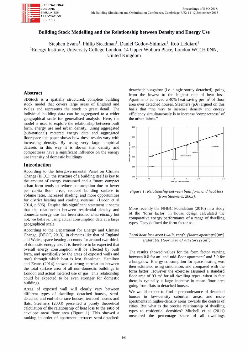
Building Stock Modelling and the Relationship between Density and Energy Use

Stephen Evans1, Philip Steadman1, Daniel Godoy-Shimizu1, Rob Liddiard1 1Energy Institute, University College London, 14 Upper Woburn Place, London WC1H 0NN,

United Kingdom

Abstract

3DStock is a spatially structured, complete building

stock model that covers large areas of England and

Wales and represents the stock in great detail. The

individual building data can be aggregated to a wider

geographical scale for generalised analysis. Here, the

model is used to explore the relationship between built

form, energy use and urban density. Using aggregated

(sub-national) metered energy data and aggregated

floorspace this paper shows how these results vary with

increasing density. By using very large empirical

datasets in this way it is shown that density and

compactness have a significant influence on the energy

use intensity of domestic buildings.

Introduction

According to the Intergovernmental Panel on Climate

Change (IPCC), the structure of a building itself is key to

the amount of energy consumed and a “more compact

urban form tends to reduce consumption due to lower

per capita floor areas, reduced building surface to

volume ratio, increased shading, and more opportunities

for district heating and cooling systems” (Lucon et al

2014, p.696). Despite this significant statement it seems

that the relationship between residential density and

domestic energy use has been studied theoretically but

not, we believe, using actual consumption data at a large

geographical scale.

According to the Department for Energy and Climate

Change, (DECC, 2013), in climates like that of England

and Wales, space heating accounts for around two-thirds

of domestic energy use. It is therefore to be expected that

overall energy consumption will be affected by built

form, and specifically by the areas of exposed walls and

roofs through which heat is lost. Steadman, Hamilton

and Evans (2014) showed a strong correlation between

the total surface area of all non-domestic buildings in

London and actual metered use of gas. This relationship

could be expected to be even stronger for domestic

buildings.

Areas of exposed wall will clearly vary between

different types of dwelling: detached houses, semi-

detached and end-of-terrace houses, terraced houses and

flats. Steemers (2003) presented a purely theoretical

calculation of the relationship of heat loss to the ratio of

envelope area/ floor area (Figure 1). This showed a

ranking in order of apartment: terrace: semi-detached:

detached: bungalow (i.e. single-storey detached), going

from the lowest to the highest rate of heat loss.

Apartments achieved a 40% heat saving per m2 of floor

area over detached houses. Steemers (p.6) argued on this

basis that “the way to increase density and energy

efficiency simultaneously is to increase ‘compactness’ of

the urban fabric.”

Figure 1: Relationship between built form and heat loss

(from Steemers, 2003).

More recently the NHBC Foundation (2016) in a study

of the ‘form factor’ in house design calculated the

comparative energy performance of a range of dwelling

types. They defined the form factor as:

𝑇𝑜𝑡𝑎𝑙 ℎ𝑒𝑎𝑡 𝑙𝑜𝑠𝑠 𝑎𝑟𝑒𝑎 (𝑤𝑎𝑙𝑙𝑠, 𝑟𝑜𝑜𝑓𝑠, 𝑓𝑙𝑜𝑜𝑟𝑠, 𝑜𝑝𝑒𝑛𝑖𝑛𝑔𝑠)(𝑚2)

𝐻𝑎𝑏𝑖𝑡𝑎𝑏𝑙𝑒 𝑓𝑙𝑜𝑜𝑟 𝑎𝑟𝑒𝑎 𝑜𝑓 𝑎𝑙𝑙 𝑠𝑡𝑜𝑟𝑒𝑦𝑠(𝑚2)

The results showed values for the form factor varying

between 0.8 for an ‘end mid-floor apartment’ and 3.0 for

a bungalow. Energy consumption for space heating was

then estimated using simulation, and compared with the

form factor. However the exercise assumed a standard

floor area of 93 m2 for all dwelling types, when in fact

there is typically a large increase in mean floor area

going from flats to detached houses.

We would expect to find a preponderance of detached

houses in low-density suburban areas, and more

apartments in higher-density areas towards the centres of

cities. But what is the precise relationship of dwelling

types to residential densities? Mitchell et al (2011)

measured the percentage share of all dwellings

Proceedings of BSO 2018: 4th Building Simulation and Optimization Conference, Cambridge, UK: 11-12 September 2018

161

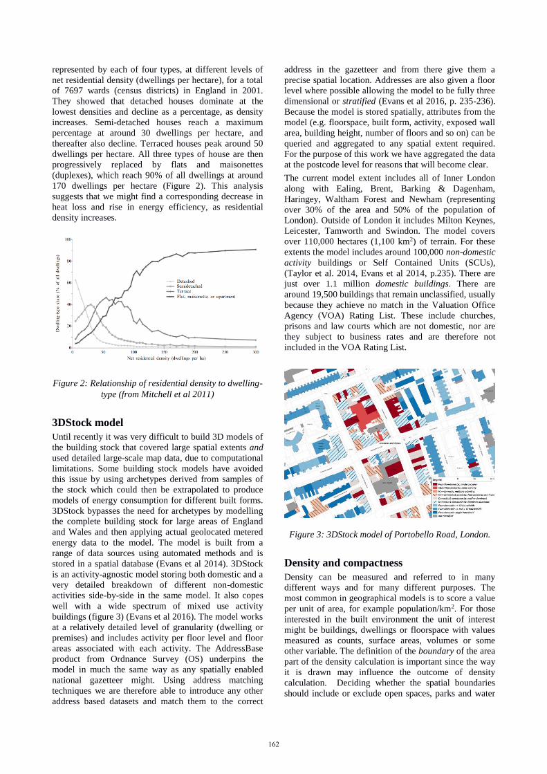
represented by each of four types, at different levels of

net residential density (dwellings per hectare), for a total

of 7697 wards (census districts) in England in 2001.

They showed that detached houses dominate at the

lowest densities and decline as a percentage, as density

increases. Semi-detached houses reach a maximum

percentage at around 30 dwellings per hectare, and

thereafter also decline. Terraced houses peak around 50

dwellings per hectare. All three types of house are then

progressively replaced by flats and maisonettes

(duplexes), which reach 90% of all dwellings at around

170 dwellings per hectare (Figure 2). This analysis

suggests that we might find a corresponding decrease in

heat loss and rise in energy efficiency, as residential

density increases.

Figure 2: Relationship of residential density to dwelling-

type (from Mitchell et al 2011)

3DStock model

Until recently it was very difficult to build 3D models of

the building stock that covered large spatial extents and

used detailed large-scale map data, due to computational

limitations. Some building stock models have avoided

this issue by using archetypes derived from samples of

the stock which could then be extrapolated to produce

models of energy consumption for different built forms.

3DStock bypasses the need for archetypes by modelling

the complete building stock for large areas of England

and Wales and then applying actual geolocated metered

energy data to the model. The model is built from a

range of data sources using automated methods and is

stored in a spatial database (Evans et al 2014). 3DStock

is an activity-agnostic model storing both domestic and a

very detailed breakdown of different non-domestic

activities side-by-side in the same model. It also copes

well with a wide spectrum of mixed use activity

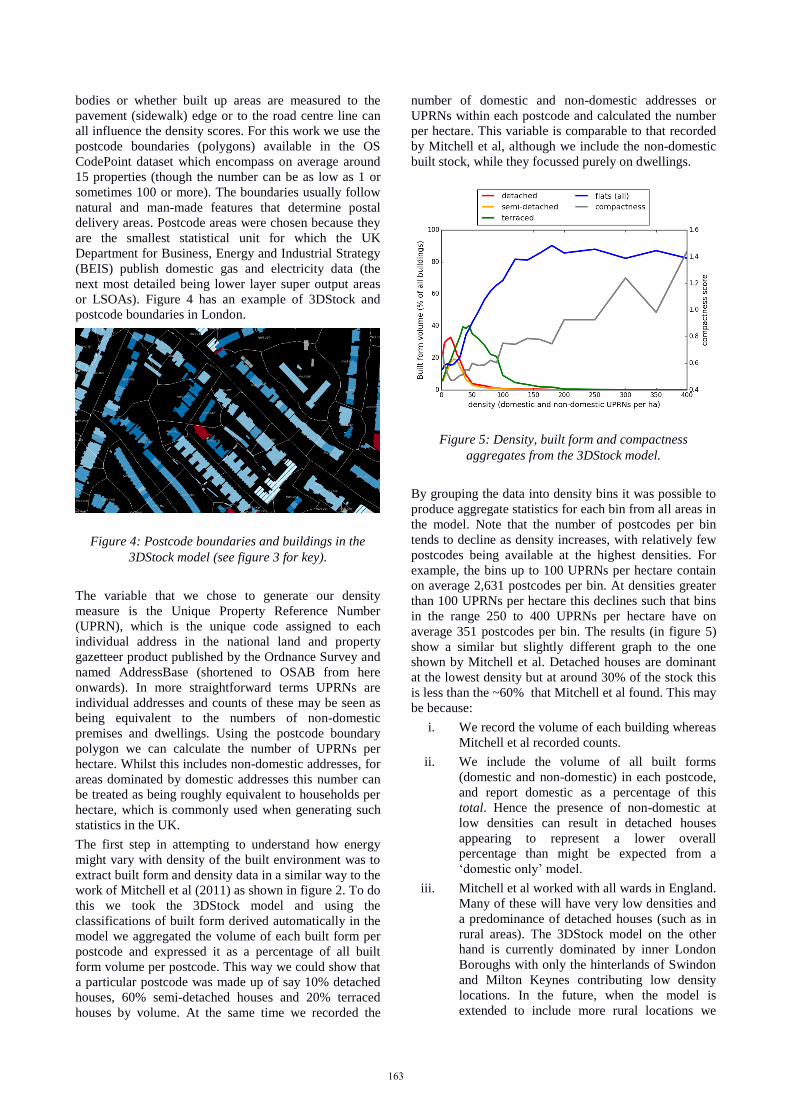
buildings (figure 3) (Evans et al 2016). The model works

at a relatively detailed level of granularity (dwelling or

premises) and includes activity per floor level and floor

areas associated with each activity. The AddressBase

product from Ordnance Survey (OS) underpins the

model in much the same way as any spatially enabled

national gazetteer might. Using address matching

techniques we are therefore able to introduce any other

address based datasets and match them to the correct

address in the gazetteer and from there give them a

precise spatial location. Addresses are also given a floor

level where possible allowing the model to be fully three

dimensional or stratified (Evans et al 2016, p. 235-236).

Because the model is stored spatially, attributes from the

model (e.g. floorspace, built form, activity, exposed wall

area, building height, number of floors and so on) can be

queried and aggregated to any spatial extent required.

For the purpose of this work we have aggregated the data

at the postcode level for reasons that will become clear.

The current model extent includes all of Inner London

along with Ealing, Brent, Barking & Dagenham,

Haringey, Waltham Forest and Newham (representing

over 30% of the area and 50% of the population of

London). Outside of London it includes Milton Keynes,

Leicester, Tamworth and Swindon. The model covers

over 110,000 hectares (1,100 km2) of terrain. For these

extents the model includes around 100,000 non-domestic

activity buildings or Self Contained Units (SCUs),

(Taylor et al. 2014, Evans et al 2014, p.235). There are

just over 1.1 million domestic buildings. There are

around 19,500 buildings that remain unclassified, usually

because they achieve no match in the Valuation Office

Agency (VOA) Rating List. These include churches,

prisons and law courts which are not domestic, nor are

they subject to business rates and are therefore not

included in the VOA Rating List.

Figure 3: 3DStock model of Portobello Road, London.

Density and compactness

Density can be measured and referred to in many

different ways and for many different purposes. The

most common in geographical models is to score a value

per unit of area, for example population/km2. For those

interested in the built environment the unit of interest

might be buildings, dwellings or floorspace with values

measured as counts, surface areas, volumes or some

other variable. The definition of the boundary of the area

part of the density calculation is important since the way

it is drawn may influence the outcome of density

calculation. Deciding whether the spatial boundaries

should include or exclude open spaces, parks and water

162

bodies or whether built up areas are measured to the

pavement (sidewalk) edge or to the road centre line can

all influence the density scores. For this work we use the

postcode boundaries (polygons) available in the OS

CodePoint dataset which encompass on average around

15 properties (though the number can be as low as 1 or

sometimes 100 or more). The boundaries usually follow

natural and man-made features that determine postal

delivery areas. Postcode areas were chosen because they

are the smallest statistical unit for which the UK

Department for Business, Energy and Industrial Strategy

(BEIS) publish domestic gas and electricity data (the

next most detailed being lower layer super output areas

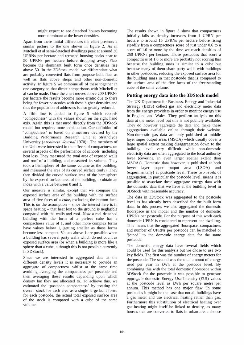
or LSOAs). Figure 4 has an example of 3DStock and

postcode boundaries in London.

Figure 4: Postcode boundaries and buildings in the

3DStock model (see figure 3 for key).

The variable that we chose to generate our density

measure is the Unique Property Reference Number

(UPRN), which is the unique code assigned to each

individual address in the national land and property

gazetteer product published by the Ordnance Survey and

named AddressBase (shortened to OSAB from here

onwards). In more straightforward terms UPRNs are

individual addresses and counts of these may be seen as

being equivalent to the numbers of non-domestic

premises and dwellings. Using the postcode boundary

polygon we can calculate the number of UPRNs per

hectare. Whilst this includes non-domestic addresses, for

areas dominated by domestic addresses this number can

be treated as being roughly equivalent to households per

hectare, which is commonly used when generating such

statistics in the UK.

The first step in attempting to understand how energy

might vary with density of the built environment was to

extract built form and density data in a similar way to the

work of Mitchell et al (2011) as shown in figure 2. To do

this we took the 3DStock model and using the

classifications of built form derived automatically in the

model we aggregated the volume of each built form per

postcode and expressed it as a percentage of all built

form volume per postcode. This way we could show that

a particular postcode was made up of say 10% detached

houses, 60% semi-detached houses and 20% terraced

houses by volume. At the same time we recorded the

number of domestic and non-domestic addresses or

UPRNs within each postcode and calculated the number

per hectare. This variable is comparable to that recorded

by Mitchell et al, although we include the non-domestic

built stock, while they focussed purely on dwellings.

Figure 5: Density, built form and compactness

aggregates from the 3DStock model.

By grouping the data into density bins it was possible to

produce aggregate statistics for each bin from all areas in

the model. Note that the number of postcodes per bin

tends to decline as density increases, with relatively few

postcodes being available at the highest densities. For

example, the bins up to 100 UPRNs per hectare contain

on average 2,631 postcodes per bin. At densities greater

than 100 UPRNs per hectare this declines such that bins

in the range 250 to 400 UPRNs per hectare have on

average 351 postcodes per bin. The results (in figure 5)

show a similar but slightly different graph to the one

shown by Mitchell et al. Detached houses are dominant

at the lowest density but at around 30% of the stock this

is less than the ~60% that Mitchell et al found. This may

be because:

i. We record the volume of each building whereas

Mitchell et al recorded counts.

ii. We include the volume of all built forms

(domestic and non-domestic) in each postcode,

and report domestic as a percentage of this

total. Hence the presence of non-domestic at

low densities can result in detached houses

appearing to represent a lower overall

percentage than might be expected from a

‘domestic only’ model.

iii. Mitchell et al worked with all wards in England.

Many of these will have very low densities and

a predominance of detached houses (such as in

rural areas). The 3DStock model on the other

hand is currently dominated by inner London

Boroughs with only the hinterlands of Swindon

and Milton Keynes contributing low density

locations. In the future, when the model is

extended to include more rural locations we

163

might expect to see detached houses becoming

more dominant at the lower densities.

Apart from these initial differences the chart presents a

similar picture to the one shown in figure 2. As in

Mitchell et al semi-detached dwellings peak at around 30

UPRNs per hectare and terraced housing peaks near to

50 UPRNs per hectare before dropping away. Flats

become the dominant built form once densities rise

above 50. In the 3DStock model we differentiate what

are probably converted flats from purpose built flats as

well as flats above shops and other non-domestic

activity. In figure 5 we combine all of these together in

one category so that direct comparisons with Mitchell et

al can be made. Once the chart moves above 200 UPRNs

per hectare the results become more erratic due to there

being far fewer postcodes with these higher densities and

thus the population of addresses is also greatly reduced.

A fifth line is added to figure 5 which records

‘compactness’ with the values shown on the right hand

axis. Again this is measured directly from the 3DStock

model but requires more explanation. Our definition of

‘compactness’ is based on a measure devised by the

Building Performance Research Unit at Strathclyde

University (Architects’ Journal 1970). The members of

the Unit were interested in the effects of compactness on

several aspects of the performance of schools, including

heat loss. They measured the total area of exposed walls

and roof of a building, and measured its volume. They

took a hemisphere of the same volume as the building,

and measured the area of its curved surface (only). They

then divided the curved surface area of the hemisphere

by the exposed surface area of the building, to obtain an

index with a value between 0 and 1.

Our measure is similar, except that we compare the

exposed surface area of the building with the surface

area of five faces of a cube, excluding the bottom face.

This is on the assumption – since the interest here is in

space heating – that heat lost to the ground is negligible

compared with the walls and roof. Now a real detached

building with the form of a perfect cube has a

compactness value of 1, and other more complex forms

have values below 1, getting smaller as those forms

become less compact. Values above 1 are possible when

a building has several party walls which do not count as

exposed surface area (or when a building is more like a

sphere than a cube, although this is not possible currently

in 3DStock).

Since we are interested in aggregated data at the

different density levels it is necessary to provide an

aggregate of compactness whilst at the same time

avoiding averaging the compactness per postcode and

then averaging these results depending upon which

density bin they are allocated to. To achieve this, we

estimated the ‘postcode compactness’ by treating the

overall stock for each area as a single large built form:

for each postcode, the actual total exposed surface area

of the stock is compared with a cube of the same

volume.

The results shown in figure 5 show that compactness

initially falls as density increases from 1 UPRN per

hectare to around 15 UPRNs per hectare before rising

steadily from a compactness score of just under 0.6 to a

score of 1.0 or more by the time we reach densities of

250 UPRNs per hectare. Those postcodes that score a

compactness of 1.0 or more are probably not scoring this

because the building mass is similar to a cube but

because many of them share party walls with buildings

in other postcodes, reducing the exposed surface area for

the building mass in that postcode that is compared to

the surface area of the five faces of the free-standing

cube of the same volume.

Putting energy data into the 3DStock model

The UK Department for Business, Energy and Industrial

Strategy (BEIS) collect gas and electricity meter data

from the energy providers in order to monitor energy use

in England and Wales. They perform analysis on this

data at the meter level but this is not publicly available.

They do however aggregate the data and make these

aggregations available online through their website.

Non-domestic gas data are only published at middle

layer super output areas (MSOA) which usually cover a

large spatial extent making disaggregation down to the

building level very difficult while non-domestic

electricity data are often aggregated to the local authority

level (covering an even larger spatial extent than

MSOAs). Domestic data however is published at both

lower layer super output area (LSOA) and

(experimentally) at postcode level. These two levels of

aggregation, in particular the postcode level, means it is

possible to associate these aggregate energy data with

the domestic data that we have at the building level in

3DStock with reasonable accuracy.

The data in 3DStock was aggregated to the postcode

level as has already been described for the built form

data. In this process we also aggregated the domestic

floorspace in the model and the number of domestic

UPRNs per postcode. For the purpose of this work each

domestic UPRN is considered to represent one dwelling.

This means that the aggregated floorspace, compactness

and number of UPRNs per postcode can be matched or

‘joined’ to the domestic energy data for the same

postcode.

The domestic energy data have several fields which

could be used for this analysis but we chose to use two

key fields. The first was the number of energy meters for

the postcode. The second was the total amount of energy

used per year in kWh at the postcode level. By

combining this with the total domestic floorspace within

3DStock for the postcode it was possible to generate

aggregate domestic Energy Use Intensity (EUI) values

at the postcode level as kWh per square metre per

annum. This method has one major flaw. In some

postcodes it might be the case that not all buildings have

a gas meter and use electrical heating rather than gas.

Furthermore this substitution of electrical heating over

gas heating might itself be linked to density, as many

houses that are converted to flats in urban areas choose

164

to use electrical heating. This is noted in an Ofgem

report which states that 25% of all flats in Great Britain

use electricity for heating, compared to only 4% of

houses (Ofgem, 2015, p.19). Another issue is that BEIS

is not allowed to publish individual meter data, yet some

postcodes may be small enough to contain only one gas

meter. This means that some data are suppressed by

BEIS to prevent disclosure of individual meter data in

these postcodes.

Added to this the method of classifying gas meters as

either domestic or non-domestic depends not on the type

of building they are attached to, but their total annual

consumption (BEIS, 2018, p.21): when their annual

consumption is above 73,200kWh per annum they are

classified as non-domestic whilst below this threshold

they are considered to be domestic. By studying the

numbers of domestic gas meters (in the aggregate

postcode statistics) in some areas with purpose built

blocks of flats it has become clear that some of these

blocks are served by one gas meter which feeds a boiler

which then provides heating to all flats in the block on a

communal basis. Because the total consumption is large

these meters are not included in the published domestic

gas data. Conversely, buildings with small non-domestic

activity such as small offices, shops and estate agents

might be heated by gas but with annual consumption that

is below the 73,200kWh and hence included in the

domestic statistics. BEIS acknowledges the latter (stating

that 500,000 non-domestic meters may be wrongly

classified as domestic p.21), but they do not

acknowledge the former not being classified as domestic.

There should not be a similar problem with electric

meters since these are usually classified by their end use

(Profile Class) rather than their level of consumption,

although there may be a few cases where activity has

switched between domestic and non-domestic but

somehow the energy companies have not been informed

of the change.

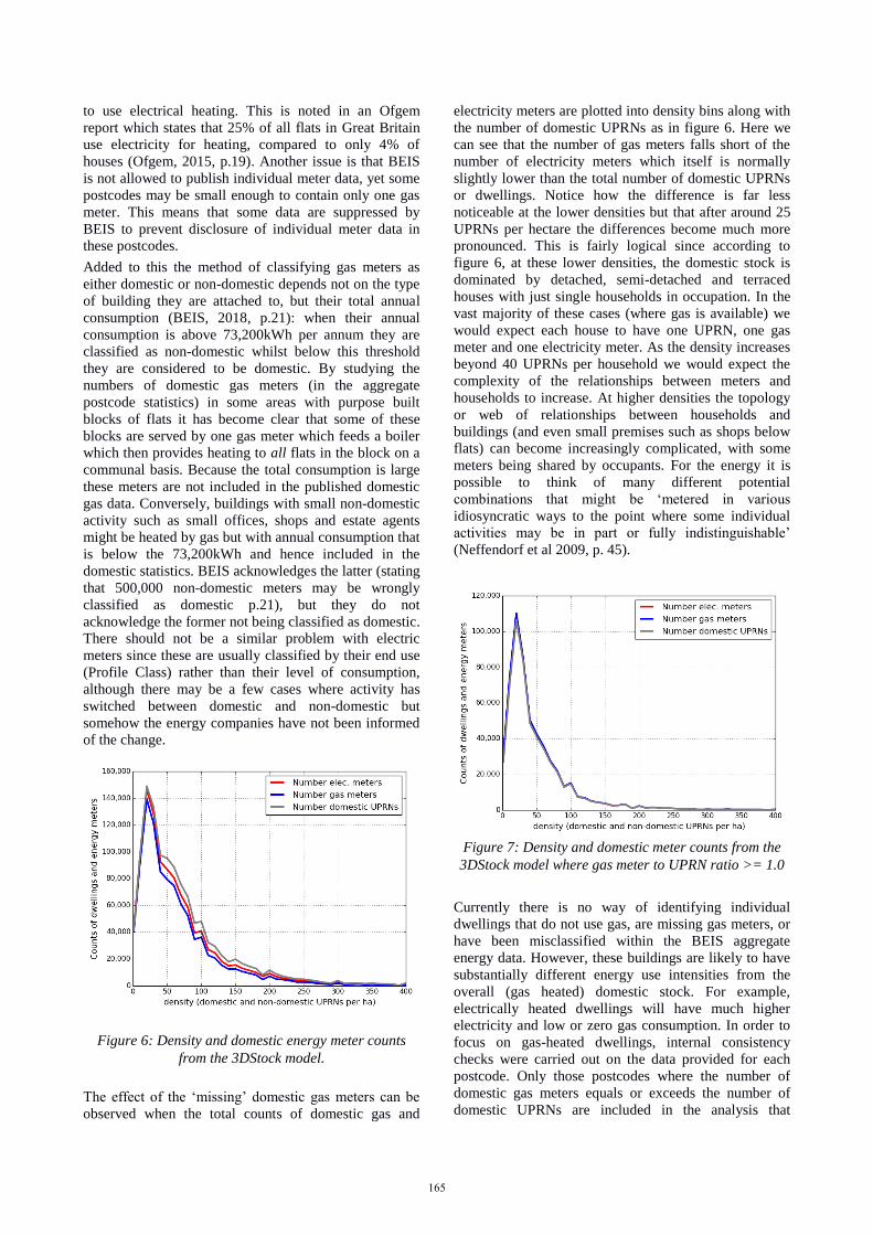
Figure 6: Density and domestic energy meter counts

from the 3DStock model.

The effect of the ‘missing’ domestic gas meters can be

observed when the total counts of domestic gas and

electricity meters are plotted into density bins along with

the number of domestic UPRNs as in figure 6. Here we

can see that the number of gas meters falls short of the

number of electricity meters which itself is normally

slightly lower than the total number of domestic UPRNs

or dwellings. Notice how the difference is far less

noticeable at the lower densities but that after around 25

UPRNs per hectare the differences become much more

pronounced. This is fairly logical since according to

figure 6, at these lower densities, the domestic stock is

dominated by detached, semi-detached and terraced

houses with just single households in occupation. In the

vast majority of these cases (where gas is available) we

would expect each house to have one UPRN, one gas

meter and one electricity meter. As the density increases

beyond 40 UPRNs per household we would expect the

complexity of the relationships between meters and

households to increase. At higher densities the topology

or web of relationships between households and

buildings (and even small premises such as shops below

flats) can become increasingly complicated, with some

meters being shared by occupants. For the energy it is

possible to think of many different potential

combinations that might be ‘metered in various

idiosyncratic ways to the point where some individual

activities may be in part or fully indistinguishable’

(Neffendorf et al 2009, p. 45).

Figure 7: Density and domestic meter counts from the

3DStock model where gas meter to UPRN ratio >= 1.0

Currently there is no way of identifying individual

dwellings that do not use gas, are missing gas meters, or

have been misclassified within the BEIS aggregate

energy data. However, these buildings are likely to have

substantially different energy use intensities from the

overall (gas heated) domestic stock. For example,

electrically heated dwellings will have much higher

electricity and low or zero gas consumption. In order to

focus on gas-heated dwellings, internal consistency

checks were carried out on the data provided for each

postcode. Only those postcodes where the number of

domestic gas meters equals or exceeds the number of

domestic UPRNs are included in the analysis that

165

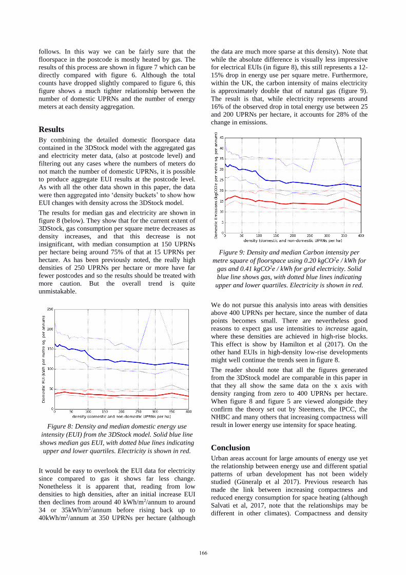
follows. In this way we can be fairly sure that the

floorspace in the postcode is mostly heated by gas. The

results of this process are shown in figure 7 which can be

directly compared with figure 6. Although the total

counts have dropped slightly compared to figure 6, this

figure shows a much tighter relationship between the

number of domestic UPRNs and the number of energy

meters at each density aggregation.

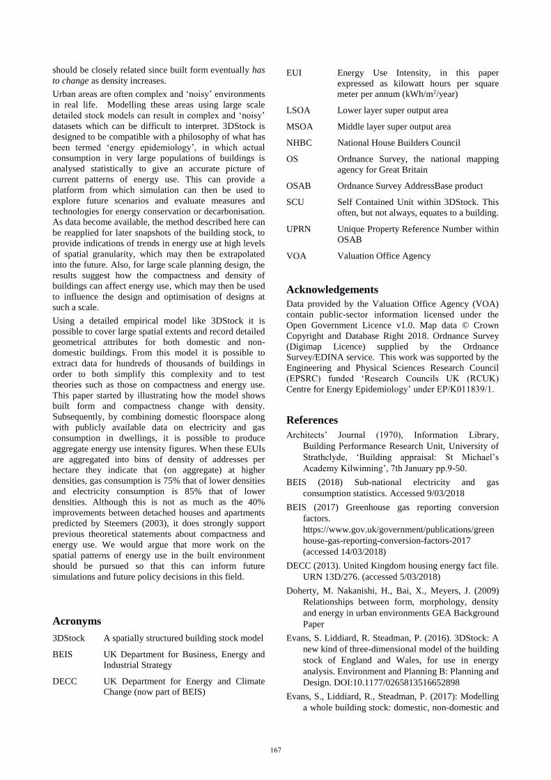
Results

By combining the detailed domestic floorspace data

contained in the 3DStock model with the aggregated gas

and electricity meter data, (also at postcode level) and

filtering out any cases where the numbers of meters do

not match the number of domestic UPRNs, it is possible

to produce aggregate EUI results at the postcode level.

As with all the other data shown in this paper, the data

were then aggregated into ‘density buckets’ to show how

EUI changes with density across the 3DStock model.

The results for median gas and electricity are shown in

figure 8 (below). They show that for the current extent of

3DStock, gas consumption per square metre decreases as

density increases, and that this decrease is not

insignificant, with median consumption at 150 UPRNs

per hectare being around 75% of that at 15 UPRNs per

hectare. As has been previously noted, the really high

densities of 250 UPRNs per hectare or more have far

fewer postcodes and so the results should be treated with

more caution. But the overall trend is quite

unmistakable.

Figure 8: Density and median domestic energy use

intensity (EUI) from the 3DStock model. Solid blue line

shows median gas EUI, with dotted blue lines indicating

upper and lower quartiles. Electricity is shown in red.

It would be easy to overlook the EUI data for electricity

since compared to gas it shows far less change.

Nonetheless it is apparent that, reading from low

densities to high densities, after an initial increase EUI

then declines from around 40 kWh/m2/annum to around

34 or 35kWh/m2/annum before rising back up to

40kWh/m2/annum at 350 UPRNs per hectare (although

the data are much more sparse at this density). Note that

while the absolute difference is visually less impressive

for electrical EUIs (in figure 8), this still represents a 12-

15% drop in energy use per square metre. Furthermore,

within the UK, the carbon intensity of mains electricity

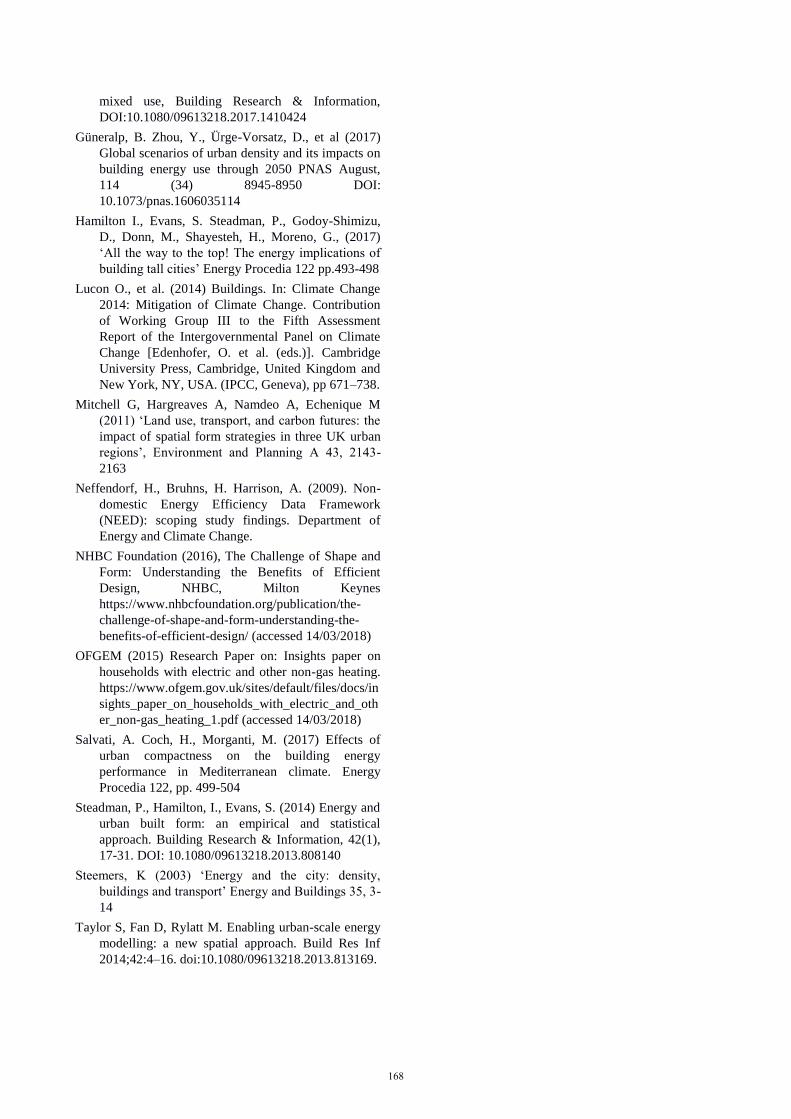
is approximately double that of natural gas (figure 9).

The result is that, while electricity represents around

16% of the observed drop in total energy use between 25

and 200 UPRNs per hectare, it accounts for 28% of the

change in emissions.

Figure 9: Density and median Carbon intensity per

metre square of floorspace using 0.20 kgCO2e / kWh for

gas and 0.41 kgCO2e / kWh for grid electricity. Solid

blue line shows gas, with dotted blue lines indicating

upper and lower quartiles. Electricity is shown in red.

We do not pursue this analysis into areas with densities

above 400 UPRNs per hectare, since the number of data

points becomes small. There are nevertheless good

reasons to expect gas use intensities to increase again,

where these densities are achieved in high-rise blocks.

This effect is show by Hamilton et al (2017). On the

other hand EUIs in high-density low-rise developments

might well continue the trends seen in figure 8.

The reader should note that all the figures generated

from the 3DStock model are comparable in this paper in

that they all show the same data on the x axis with

density ranging from zero to 400 UPRNs per hectare.

When figure 8 and figure 5 are viewed alongside they

confirm the theory set out by Steemers, the IPCC, the

NHBC and many others that increasing compactness will

result in lower energy use intensity for space heating.

Conclusion

Urban areas account for large amounts of energy use yet

the relationship between energy use and different spatial

patterns of urban development has not been widely

studied (Güneralp et al 2017). Previous research has

made the link between increasing compactness and

reduced energy consumption for space heating (although

Salvati et al, 2017, note that the relationships may be

different in other climates). Compactness and density

166

should be closely related since built form eventually has

to change as density increases.

Urban areas are often complex and ‘noisy’ environments

in real life. Modelling these areas using large scale

detailed stock models can result in complex and ‘noisy’

datasets which can be difficult to interpret. 3DStock is

designed to be compatible with a philosophy of what has

been termed ‘energy epidemiology’, in which actual

consumption in very large populations of buildings is

analysed statistically to give an accurate picture of

current patterns of energy use. This can provide a

platform from which simulation can then be used to

explore future scenarios and evaluate measures and

technologies for energy conservation or decarbonisation.

As data become available, the method described here can

be reapplied for later snapshots of the building stock, to

provide indications of trends in energy use at high levels

of spatial granularity, which may then be extrapolated

into the future. Also, for large scale planning design, the

results suggest how the compactness and density of

buildings can affect energy use, which may then be used

to influence the design and optimisation of designs at

such a scale.

Using a detailed empirical model like 3DStock it is

possible to cover large spatial extents and record detailed

geometrical attributes for both domestic and non-

domestic buildings. From this model it is possible to

extract data for hundreds of thousands of buildings in

order to both simplify this complexity and to test

theories such as those on compactness and energy use.

This paper started by illustrating how the model shows

built form and compactness change with density.

Subsequently, by combining domestic floorspace along

with publicly available data on electricity and gas

consumption in dwellings, it is possible to produce

aggregate energy use intensity figures. When these EUIs

are aggregated into bins of density of addresses per

hectare they indicate that (on aggregate) at higher

densities, gas consumption is 75% that of lower densities

and electricity consumption is 85% that of lower

densities. Although this is not as much as the 40%

improvements between detached houses and apartments

predicted by Steemers (2003), it does strongly support

previous theoretical statements about compactness and

energy use. We would argue that more work on the

spatial patterns of energy use in the built environment

should be pursued so that this can inform future

simulations and future policy decisions in this field.

Acronyms

3DStock A spatially structured building stock model

BEIS UK Department for Business, Energy and

Industrial Strategy

DECC UK Department for Energy and Climate

Change (now part of BEIS)

EUI Energy Use Intensity, in this paper

expressed as kilowatt hours per square

meter per annum (kWh/m2/year)

LSOA Lower layer super output area

MSOA Middle layer super output area

NHBC National House Builders Council

OS Ordnance Survey, the national mapping

agency for Great Britain

OSAB Ordnance Survey AddressBase product

SCU Self Contained Unit within 3DStock. This

often, but not always, equates to a building.

UPRN Unique Property Reference Number within

OSAB

VOA Valuation Office Agency

Acknowledgements

Data provided by the Valuation Office Agency (VOA)

contain public-sector information licensed under the

Open Government Licence v1.0. Map data © Crown

Copyright and Database Right 2018. Ordnance Survey

(Digimap Licence) supplied by the Ordnance

Survey/EDINA service. This work was supported by the

Engineering and Physical Sciences Research Council

(EPSRC) funded ‘Research Councils UK (RCUK)

Centre for Energy Epidemiology’ under EP/K011839/1.

References

Architects’ Journal (1970), Information Library,

Building Performance Research Unit, University of

Strathclyde, ‘Building appraisal: St Michael’s

Academy Kilwinning’, 7th January pp.9-50.

BEIS (2018) Sub-national electricity and gas

consumption statistics. Accessed 9/03/2018

BEIS (2017) Greenhouse gas reporting conversion

factors.

https://www.gov.uk/government/publications/green

house-gas-reporting-conversion-factors-2017

(accessed 14/03/2018)

DECC (2013). United Kingdom housing energy fact file.

URN 13D/276. (accessed 5/03/2018)

Doherty, M. Nakanishi, H., Bai, X., Meyers, J. (2009)

Relationships between form, morphology, density

and energy in urban environments GEA Background

Paper

Evans, S. Liddiard, R. Steadman, P. (2016). 3DStock: A

new kind of three-dimensional model of the building

stock of England and Wales, for use in energy

analysis. Environment and Planning B: Planning and

Design. DOI:10.1177/0265813516652898

Evans, S., Liddiard, R., Steadman, P. (2017): Modelling

a whole building stock: domestic, non-domestic and

167

mixed use, Building Research & Information,

DOI:10.1080/09613218.2017.1410424

Güneralp, B. Zhou, Y., Ürge-Vorsatz, D., et al (2017)

Global scenarios of urban density and its impacts on

building energy use through 2050 PNAS August,

114 (34) 8945-8950 DOI:

10.1073/pnas.1606035114

Hamilton I., Evans, S. Steadman, P., Godoy-Shimizu,

D., Donn, M., Shayesteh, H., Moreno, G., (2017)

‘All the way to the top! The energy implications of

building tall cities’ Energy Procedia 122 pp.493-498

Lucon O., et al. (2014) Buildings. In: Climate Change

2014: Mitigation of Climate Change. Contribution

of Working Group III to the Fifth Assessment

Report of the Intergovernmental Panel on Climate

Change [Edenhofer, O. et al. (eds.)]. Cambridge

University Press, Cambridge, United Kingdom and

New York, NY, USA. (IPCC, Geneva), pp 671–738.

Mitchell G, Hargreaves A, Namdeo A, Echenique M

(2011) ‘Land use, transport, and carbon futures: the

impact of spatial form strategies in three UK urban

regions’, Environment and Planning A 43, 2143-

2163

Neffendorf, H., Bruhns, H. Harrison, A. (2009). Non-

domestic Energy Efficiency Data Framework

(NEED): scoping study findings. Department of

Energy and Climate Change.

NHBC Foundation (2016), The Challenge of Shape and

Form: Understanding the Benefits of Efficient

Design, NHBC, Milton Keynes

https://www.nhbcfoundation.org/publication/the-

challenge-of-shape-and-form-understanding-the-

benefits-of-efficient-design/ (accessed 14/03/2018)

OFGEM (2015) Research Paper on: Insights paper on

households with electric and other non-gas heating.

https://www.ofgem.gov.uk/sites/default/files/docs/in

sights_paper_on_households_with_electric_and_oth

er_non-gas_heating_1.pdf (accessed 14/03/2018)

Salvati, A. Coch, H., Morganti, M. (2017) Effects of

urban compactness on the building energy

performance in Mediterranean climate. Energy

Procedia 122, pp. 499-504

Steadman, P., Hamilton, I., Evans, S. (2014) Energy and

urban built form: an empirical and statistical

approach. Building Research & Information, 42(1),

17-31. DOI: 10.1080/09613218.2013.808140

Steemers, K (2003) ‘Energy and the city: density,

buildings and transport’ Energy and Buildings 35, 3-

14

Taylor S, Fan D, Rylatt M. Enabling urban-scale energy

modelling: a new spatial approach. Build Res Inf

2014;42:4–16. doi:10.1080/09613218.2013.813169.

168