


Languages
Pages
Legal

National Poverty Center Working Paper Series
#09-05
March 2009
The Information Theory of Segregation: Uniting Segregation and
Inequality in a Common Framework
Paul A. Jargowsky, University of Texas at Dallas
Jeongdai Kim, Green Mountain Energy Co.
This paper is available online at the National Poverty Center Working Paper Series index at:
http://www.npc.umich.edu/publications/working_papers/
Any opinions, findings, conclusions, or recommendations expressed in this material are those of the author(s) and do
not necessarily reflect the view of the National Poverty Center or any sponsoring agency.
The Information Theory of Segregation: Uniting Segregation and
Inequality in a Common Framework*
Paul A. Jargowsky
University of Texas at Dallas GR31
2601 N. Floyd Rd.
Richardson, TX
Jeongdai Kim
Green Mountain Energy Co.
March 4, 2009
*An earlier version of this paper was presented at the conference, “New Frontiers in the
Field of Segregation Measurement and Analysis,” July 3-8, 2007, in Monte Verita,
Switzerland. We are grateful to Nathan Berg, Brian Berry, Marie Chevrier, Euel Elliott,
Yves Flückiger, Christopher Jencks, Murray Leaf, Sean Riordan, Jacques Silber, and the
conference participants for helpful comments and discussions. Please direct comments to
[email protected] and/or [email protected].

The Information Theory of Segregation: Uniting Segregation and
Inequality in a Common Framework
Abstract
Drawing on insights from Shannon’s (1948) seminal paper on Information Theory, we
propose that all measures of segregation and inequality are united within a single
conceptual framework. We argue that segregation is fundamentally analogous to the loss
of information from an aggregation process. Integration is information loss and
segregation is information retention. Specifying the exact theoretical and mathematical
relationship between inequality and segregation measures is useful for several reasons. It
highlights the common mathematical structure shared by many different segregation
measures, and it suggests certain useful variants of these measures that have not been
recognized previously. We develop several new measures, including a Gini Segregation
Index (GS) for continuous variables and Income Dissimilarity (ID), a version of the Index
of Dissimilarity suitable for measuring economic segregation. We also show that
segregation measures can easily be adapted to handle persons of mixed race, and describe
the Non-Exclusive Index of Dissimilarity (NED) and the Non-Exclusive Entropy Index
of Segregation (NEH). We also develop a correction for structural constraints on the
value of segregation measures, comparable to capacity constraints in a communications
channel, that prevent them reaching their theoretical maximum or minimum value.

- 1 -
The Information Theory of Segregation: Uniting Segregation and
Inequality in a Common Framework
Introduction
Shannon’s landmark paper, “The Mathematical Theory of Communication”
(1948), examined the problems of transmitting information over limited and potentially
noisy channels. The paper, which has been cited over 20,000 times, launched the field of
Information Theory and is considered foundational in several disciplines, including
communications, digital computing, and cryptography. Previous work in the
measurement of segregation has drawn on information theory measures and concepts, but
only to a limited extent. We propose a much more direct and fundamental connection
between segregation and information theory, one that unites measures of segregation and
inequality in a single framework. Specifically, we argue that the question of segregation
is analogous to the problem of communicating information over a noisy channel.
We propose an Information Theory of Segregation that defines segregation in
terms of the ratio of inequality among individuals to inequality between groups of
individuals, e.g. neighborhoods. We state four specific propositions concerning
inequality and segregation measures that follow from this approach, and discuss the
implications of these propositions. As result of the application of information theory to
the question of segregation, we are able to develop several important results. First, all
inequality measures can be used to form segregation measures. Second, most commonly
used segregation measures can be expressed as the ratio of two inequality measures.
- 2 -
Third, we show that several segregation measures that cannot be expressed this way are
not measures of segregation at all, but rather measures of neighborhood inequality.
Fourth, by understanding their common mathematical structure, segregation measures
which were previously used only in the binary case are shown to have analogues that are
applicable to continuous variables, such as income. Fifth, insights generated by this
approach show how racial segregation measures can be applied to situations involving
mixed race individuals, such as Tiger Woods or Barack Obama.
Our goal in this paper is to provide a conceptual foundation for segregation
measures based on Information Theory. Not all measures of segregation that have been
proposed are consistent with the framework developed here. Researchers are obviously
free to adopt a different or broader conceptualization of the meaning of segregation.
However, the clarity and new insights generated by the Information Theory approach are
strong arguments in its favor.
Information Theory, Segregation, and Inequality
Shannon wrote that “the fundamental problem of communication is that of
reproducing at one point…a message selected at another point” (1948: 379). A
communication system consists of an information source, a destination, and a possibly
noisy transmission process over a medium that has limited capacity, such as a telephone
cable. Defining the information content of the source was the crucial first step to
Shannon’s analysis. He characterized the information value of a source as a function of
the number of potential messages, or different states of the system, that the source could
produce. The technical problem in the field of communication is whether the intended
recipient of a message can distinguish it from among the many possible messages that the
- 3 -
sender could have sent. Communication is only a problem if the receiver is uncertain
about what message the source intends. The more potential messages, i.e. the greater the
information content of the source, the greater the uncertainty about the intended message.
Therefore, the information content of the source is at a minimum if there is only one
possible message, and increases as the number of possible messages and therefore the
uncertainty about any specific message increases.
All of this may seem far removed from the issues of inequality and segregation,
yet we argue that this perspective is directly applicable. We conceptualize the source as
information about a population of individuals, specifically the values of a particular
variable that characterizes the individuals. The information content of the source is the
variation between individuals. If individuals are identical, then choosing an individual at
random will produce the same message every time. In Shannon’s terms, the information
of the source is zero because there is no uncertainty about the message. If there is a great
deal of variation among the individuals, then there are many possible messages that can
be produced (many different “states of the system”) and the information value of the
source is high.
The communication process is analogous to the sorting into groups. For example,
the groups can be a two-dimensional grid of neighborhoods. The message received is
contained in a set of values, one for each group, which characterizes the individuals in the
group. Usually, but not necessarily, that value is the mean of the variable for the
individuals in that group. The message also contains the number of individuals in each
group. After the sorting takes place, the information content of the message received
depends on the resulting distribution of neighborhood values of the outcome variable. If
- 4 -
all the groups have the same mean, the sorting process destroyed all of the information
about the underlying distribution of the variable at the level of individuals. In certain
circumstances, all of the information about the underlying distribution might be
preserved.
Imagine a Martian attempting to learn about income inequality in a certain city.
The Martian goes to the Census Bureau, which gives him a vector of mean incomes for
census tracts and the populations of those tracts but no information on individuals. If all
the neighborhood means are identical, the Martian can say nothing about the underlying
distribution of income. However, if each person lives in a neighborhood with persons of
identical income, then all the information from the original income distribution was
preserved, including the total number of individuals at each income level. The former
situation represents a state of integration, the latter represents extreme segregation.1
The Information Theory of Segregation, therefore, holds that segregation and
inequality have a very specific relationship. Inequality is information about variation in
an outcome of interest. Segregation is the degree of preservation of that information after
a grouping process. Integration is the destruction of information about inequality by
grouping. Segregation should therefore be measured by comparing the information
about inequality available in the group summary data to the information about inequality
in the individual-level data. Information may be measured in many different ways, but
the same measure of inequality should be applied to the group-level data as to the
individual-level data, so that the degree of “equivocation” in the signal is due to the
grouping process and not differences in weighting or measurement.
1 The argument also applies to binary variables, as will be demonstrated below.

- 5 -
Although there are specific mathematical relationships implied by this perspective
on segregation, as discussed in detail below, the point is entirely conceptual. The
Information Theory of Segregation should be adopted if the perspective it offers proves
compelling and useful. We argue that an information theory perspective on segregation
clarifies the relationships between many measures of inequality and measures of
segregation and that it solves problems in the measurement of segregation, such as how
to handle multi-racial individuals or how to apply several traditional segregation
measures to continuous variables.
Notation and Assumptions
For the purpose of illustration and to set notation, we assume a finite population
composed of N individuals. They could be people or households or corporations or trees
in the forest, but for the purpose of this analysis we assume they are indivisible. The
individuals have a characteristic of interest, which is the value of a variable Yi, where i
indexes individuals from 1 to N. If two subscripts are needed, we use h and i to index
individuals. Each individual is a member of a group of some kind, and there are j = 1 to
M mutually exclusive and collectively exhaustive groups. If two subscripts are needed,
we use j and k to index the groups. The population sizes of the groups may be equal or
uneven, but in any case they are denoted by nj or nk. Empty groups are not allowed, and
at least one group must have more than one individual, implying that M<N. By
construction, the sum of nj equals N. The groups are typically spatial units, such as
neighborhoods, but the grouping can be any clearly defined categorization, such as social
class, caste, or occupations.
- 6 -
In some cases, the outcome variable Y is continuous, such as income. The overall
mean of Y is denoted μ and the mean for group j is μj. In other cases, the variable is
binary, such as gender or a binary race variable such as black/non-black. For a
dichotomous variable, the overall mean is P and the group mean is pj. For nominal
variables with more than two categories, such as a race or religion, we index the
categories with r ranging from 1 to R, and prj is proportion of category r in group j. With
few exceptions, subscripts denote indexes and superscripts (other than exponents) denote
qualifiers; for example, iB means the value of B for the ith
individual, but iB is a function
B calculated on the basis of individual-level data.
Measures of inequality examine the distribution of Y among the N individuals
with no regard to the M groups of which they are members. Inequality exists if and only
if some members of the population differ in terms of Y, which is equivalent to saying that
some members have incomes not equal to the central tendency of the distribution. A
measure of inequality is a single statistic that represents the degree of inequality across
the whole distribution, allowing comparisons between one distribution and another or
between the same distribution at two points in time. Many inequality measures focus on
income percentiles, i.e. deviations from the median, such as the interquartile range or the
ratio of the 90th
to the 10th
percentile. Other measures are based on deviations from the
mean, including the variance, the variance of log Y, and the Theil Index. The Gini Index
is based on the mean difference between individuals in the population. These measures
differ mainly in how they weight deviations from the central tendency (Firebaugh, 1999:
1608).
- 7 -
In contrast, measures of segregation provide a summary measure of the
differential distribution of the N individuals into the M groups according to the
characteristic Y. Y is often race, most often defined as a dichotomous variable of white
vs. black. Segregation measures abound for the binary case, but the most common is the
Index of Dissimilarity. The relationships among these measures, their properties, and
their comparative advantages have been reviewed extensively (Duncan and Duncan,
1955; Frankel and Volij, 2007; Hutchens, 2001; James and Taeuber, 1985; Massey and
Denton, 1988; White, 1986; Winship, 1977). Many have been extended to the
polytomous case (James, 1986; Morgan, 1975; Reardon and Firebaugh, 2002; Sakoda,
1981). A smaller set of measures and procedures have been used to measure segregation
when the characteristic Y is continuous, such as household income (Hardman and
Ioanides, 2004; Ioannides, 2004; Jargowsky, 1996; Massey and Eggers, 1990).
Shannon (1948) defined the entropy score (E) as the information value of a given
state of a system, but the argument here is independent of a particular measure of
information.2 In our application, the information of interest is the diversity or variation of
Y over a population of individuals. The information content of the population is zero if
and only if all members of the population are identical, in which case we are certain of
the outcome of choosing a person at random from the population. Given a set of possible
outcomes for a discrete variable or a range of possible outcomes for a continuous
variable, information is maximized when all possible values of Y are equally likely
2 Shannon (1948) actually used H to denote entropy, but in the segregation literature H is reserved for the
Entropy Index of Segregation while E usually denotes the entropy, i.e. diversity, score of groups or the
system as a whole.

- 8 -
(Shannon, 1948), i.e. a uniform distribution or equal probabilities for each category in a
binary or polytomous variable.
Segregation and inequality are closely related, as has long been recognized. If
there is no inequality (in the sense of variation between individuals), then segregation is a
moot point – segregation by what? Every member of the population is indistinguishable.
On the other hand, if inequality exists in income, race, or some other characteristic, we
can ask about the extent to which different values of the outcome are clustered in space or
sorted into certain identifiable groups. Hutchens (2001: 15), for example, states that
segregation is a form of inequality: “segregation assesses inequality in the distribution of
people across groups.” We go beyond the notion that segregation is related to inequality
among groups to defining segregation as the retention of information about inequality
when comparing the group information to the individual-level information.
Several authors have noted parallels and borrowed techniques from inequality
research to study segregation, notably Hutchens (2001, 2004), James and Taeuber (1985),
and Reardon and Firebaugh (2002). However, to our knowledge, prior researchers did
not articulate a fundamental relationship between these two concepts. Several
propositions follow from thinking about segregation as the transmission of information
about inequality over, or through, a grouping process. The first three propositions are
closely related and concern the relationship between measures of inequality and measures
of segregation. The fourth proposition concerns capacity constraints on the grouping
process that render the theoretical maximum and minimum value of segregation
unattainable. We attempt to demonstrate these propositions by showing how they apply
- 9 -
to several commonly used measures of segregation and inequality. Several new measures
and relationships among existing measures are demonstrated.
Implications of an Information Theory Approach to Segregation
In this section, we briefly outline four propositions that follow from adopting an
Information Theory approach to the conceptualization and measurement of segregation.
In the following sections, we provide support for the propositions and illustrate their
implications by examining common measures of inequality and segregation and showing
their interrelationships.
Proposition 1
For any inequality measure Φ, there is a corresponding segregation measure ,
formed by the ratio of the inequality measured at the group level to the same inequality
measure measured at the individual level. Thus,
j
i
(1)
Segregation measures formed in this way possess the inequality ratio property.
Proposition 2
Conversely, any measure of segregation can be expressed as the ratio of two
underlying inequality measures, j and i . In other words, we argue that all “valid”
measures of segregation have the inequality ratio property. Obviously, researchers are
free to define a multitude of measures and call them segregation measures, whether or not
they have the inequality ratio property. However, if one accepts the conceptual
framework we have described relating segregation and inequality through information

- 10 -
theory, Proposition 2 must hold. We argue that measures which do not possess the
inequality ratio measure are actually hybrid measures, combining an element of
segregation with other concerns.
Taken together, Propositions 1 and 2 unify the concepts of inequality and
segregation and imply a one-to-one theoretical and technical relationship between
measures of inequality and segregation.
Proposition 3
A surprising outcome of viewing segregation through Information Theory is the
finding that all measures of inequality that can be applied to either binary or continuous
variables generate measures of segregation that can be applied to either binary or
continuous variables. Thus, measures such as the Gini and Atkinson measures of
segregation that have only been applied in the binary case have forms that can be used for
continuous variables like income. Moreover, the Index of Dissimilarity, which is
normally limited to binary or polytomous variables, may be used in the analysis of
continuous variables as well.
Proposition 4
Segregation measures have a theoretical minimum of perfect integration and a
theoretical maximum for perfect segregation. However, in many cases the theoretical
limits may not be attainable for reasons that have nothing to do with segregation.
Shannon described an analogous problem regarding communication over a noisy channel
or a channel with a capacity constraint. To address this, we define two functions,
SortMax and SortMin. The SortMax is the maximum value of j that can be produced
- 11 -
given the set of group sizes {n1, n2, …, nj, … , nM} and the set of individual values of Y
{Y1, Y2, … , Yi, … , YN} and is denoted max
j . Likewise, SortMin is the minimum value
of neighborhood inequality, and is denoted min
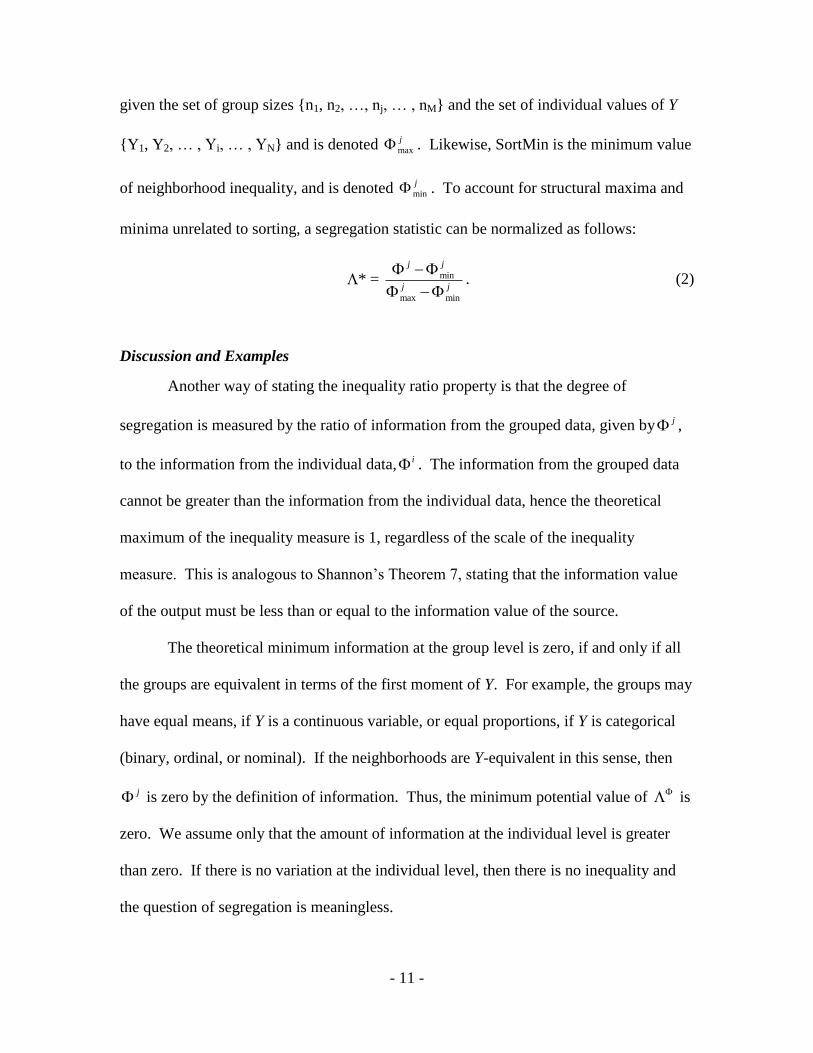
j . To account for structural maxima and
minima unrelated to sorting, a segregation statistic can be normalized as follows:
min
max min
* = j j
j j
. (2)
Discussion and Examples
Another way of stating the inequality ratio property is that the degree of
segregation is measured by the ratio of information from the grouped data, given by j ,
to the information from the individual data, i . The information from the grouped data
cannot be greater than the information from the individual data, hence the theoretical
maximum of the inequality measure is 1, regardless of the scale of the inequality
measure. This is analogous to Shannon’s Theorem 7, stating that the information value
of the output must be less than or equal to the information value of the source.
The theoretical minimum information at the group level is zero, if and only if all
the groups are equivalent in terms of the first moment of Y. For example, the groups may
have equal means, if Y is a continuous variable, or equal proportions, if Y is categorical
(binary, ordinal, or nominal). If the neighborhoods are Y-equivalent in this sense, then
j is zero by the definition of information. Thus, the minimum potential value of is
zero. We assume only that the amount of information at the individual level is greater
than zero. If there is no variation at the individual level, then there is no inequality and
the question of segregation is meaningless.
- 12 -
We illustrate Proposition 1 by discussing the correlation ratio and the application
of the Gini Index to the measurement of income segregation. In both cases, the
segregation measure is formed by a ratio of corresponding group and individual
inequality measures. We then illustrate Proposition 2 by showing that several common
segregation measures – the Index of Dissimilarity and the Entropy Index -- are also
effectively ratios of underlying inequality measures, a fact not previously recognized.
Variance Ratio Measures
The correlation ratio, also referred to as eta2 or the variance ratio, has been used
as a measure of segregation for both dichotomous and continuous variables (Bell, 1954;
Farley, 1977; Schnare, 1980; Zoloth, 1976). Reardon and Firebaugh (2002) develop a
version for multiple groups. If the j groups are census tracts, the correlation ratio “may
be thought of as a one-way analysis of variance model in which the overall variance…is
divided into within census tract and between census tract variances” (Farley, 1977: 503).
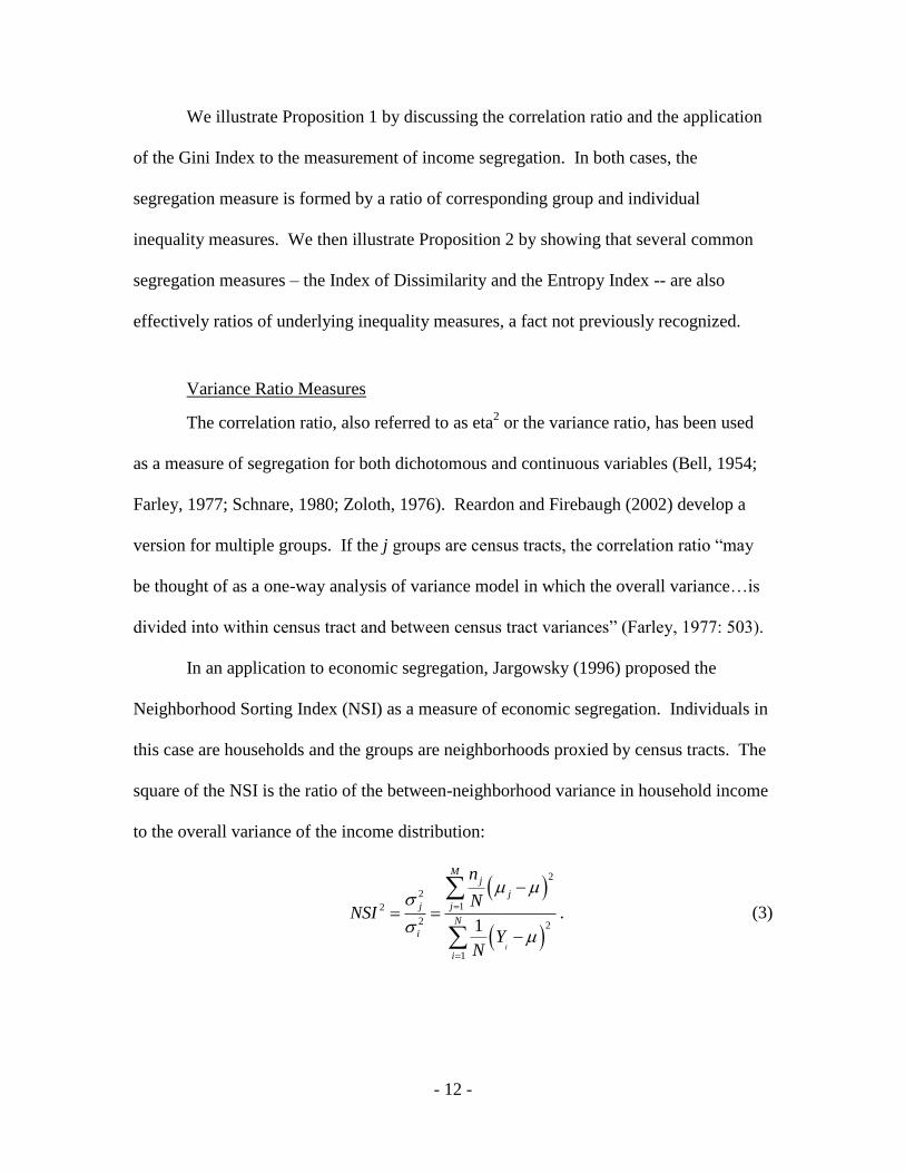
In an application to economic segregation, Jargowsky (1996) proposed the
Neighborhood Sorting Index (NSI) as a measure of economic segregation. Individuals in
this case are households and the groups are neighborhoods proxied by census tracts. The
square of the NSI is the ratio of the between-neighborhood variance in household income
to the overall variance of the income distribution:
2
2
12
2 2
1
1i
Mj
j
j j
N
i
i
n
NNSI
YN
. (3)

- 13 -
However, another way to look at this measure is simply the ratio of the variance of the j
distribution to the variance of the i distribution.3 The denominator is clearly an inequality
measure, whereas the numerator is a measure of the inequality of the grouped data,
weighted by tract population. The denominator can also be considered to be weighted,
with each individual having a weight of 1/N (Firebaugh, 1999: 1607). Thus, the NSI and
similar segregation measures are consistent with Proposition 1, because they are formed
by a measure of inequality at the group level to the same measure of inequality at the
individual level.
The Gini Segregation Coefficient (GS)
The Gini coefficient is perhaps the best known measure of inequality (Gini, 1912,
1921). Gini coefficients are routinely computed for all nations in the world that collect
adequate data (Milanovic, 2002). Several authors have employed the Gini as a measure
of segregation, but its use has been limited to dichotomous groups (Silber, 1989; James
and Tauber, 1985; Massey and Denton, 1988). Reardon and Firebaugh (2002) extended
the Gini to polytomous categorical variables and Dawkins (2004) has proposed a spatial
version.
The Gini index can be computed by a number of different formulas and
procedures (Pyatt, 1976; Silber, 1989; Yao, 1999). For our purposes, we employ the
mean difference formulation (Gini 1912, 1921) of the Gini coefficient:
2
1 1
1
2
N Ni
h i
h i
G Y YN
. (4)
3 Similar measures using other metrics have been proposed, including the ratio of neighborhood and
individual variance of log income (Ioannides, 2004) and coefficients of variation (Hardman and Ioannides,
2004).

- 14 -
The Gini measure can just as easily be applied to the smaller set of values
comprising the group or neighborhood means:
2
1 1
1
2
M Mj
j k j k
j k
G n nN
, (5)
where j and k both index groups. Kim and Jargowsky (2005) develop this index
geometrically and show that the grouped (i.e. neighborhood-level) Gini Index is always
less than or equal to the Gini computed from the individual level.
The group-level Gini Index has been used to measure the spatial distribution of
health care providers (Brown, 1994; Schwartz et al., 1980). Hutchens considered and
rejected a grouped version of the Gini as a measure of occupational segregation (2004).
The group-level Gini, however, simply measures the inequality of the groups without
conveying any information on how the distribution of Y changes when individuals are
sorted into groups. jG reaches a maximum of iG when each individual lives in a
neighborhood (or is a member of a group) with a mean income identical to their own.
When any group contains individuals of who differ in terms of Y, jG must be less than
iG .
As an example, let Y be income and consider a city with 100 neighborhoods and
200 persons, 100 of whom have an income of $9,999 and the remaining 100 of whom
have incomes of $10,001. Clearly, there is little inequality. There is complete
neighborhood equality if each neighborhood pairs a “rich” and “poor” person. There is
complete segregation if each neighborhood contains only one income level or the other.
In both, however, the group level Gini will still report a value close to zero because the

- 15 -
neighborhoods are quite similar despite the complete segregation of the rich from the
poor.
The important point is that jG is not a pure measure of segregation. The
maximum value of jG can never exceed iG . The maximum possible degree of inequality
between the M groups is limited by the amount of inequality in the original income
distribution of the N individual units. The grouping process may destroy some of the
inequality information available in the individual distribution. Segregation is a question
of organization, not degree of disparity, a distinction that does not arise the case of
nominal variables. Segregation may interact with inequality to produce worse outcomes
on a variety of important variables, but segregation and inequality are conceptually
distinct. The problem is solved by dividing the group-level Gini by the individual-level
Gini, canceling the common terms:
1 1
1 1
M M
j k j kjj kG
N Ni
h i
h i
n nG
GY Y
. (6)
We call this the Gini Segregation Index (GS). Returning to the example of the previous
paragraph, G produces zero when the rich and poor are paired and one if they are
completely segregated.
As a check on the logic of Equation 6, we simplify the Gini Segregation Index as
we have developed it to the binary case to see if it is consistent with the Gini in use in
racial segregation studies. Let Yi be an indicator variable equal to 1 for black and 0 for
white. The mean of binary variable Y becomes P, the percent black, and the mean of Y in
- 16 -
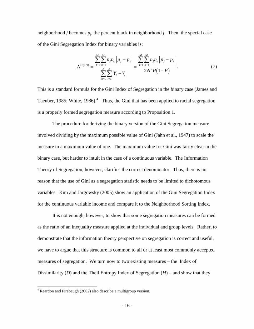
neighborhood j becomes pj, the percent black in neighborhood j. Then, the special case
of the Gini Segregation Index for binary variables is:
1 1 1 1(0/1)
2
1 1
2 1
M M M M
j k j k j k j k
j k j kG
N N
h i
h i
n n p p n n p p
N P PY Y
. (7)
This is a standard formula for the Gini Index of Segregation in the binary case (James and
Taeuber, 1985; White, 1986).4 Thus, the Gini that has been applied to racial segregation
is a properly formed segregation measure according to Proposition 1.
The procedure for deriving the binary version of the Gini Segregation measure
involved dividing by the maximum possible value of Gini (Jahn et al., 1947) to scale the
measure to a maximum value of one. The maximum value for Gini was fairly clear in the
binary case, but harder to intuit in the case of a continuous variable. The Information
Theory of Segregation, however, clarifies the correct denominator. Thus, there is no
reason that the use of Gini as a segregation statistic needs to be limited to dichotomous
variables. Kim and Jargowsky (2005) show an application of the Gini Segregation Index
for the continuous variable income and compare it to the Neighborhood Sorting Index.
It is not enough, however, to show that some segregation measures can be formed
as the ratio of an inequality measure applied at the individual and group levels. Rather, to
demonstrate that the information theory perspective on segregation is correct and useful,
we have to argue that this structure is common to all or at least most commonly accepted
measures of segregation. We turn now to two existing measures – the Index of
Dissimilarity (D) and the Theil Entropy Index of Segregation (H) – and show that they
4 Reardon and Firebaugh (2002) also describe a multigroup version.

- 17 -
are consistent with the Information Theory of Segregation, even though they have not
been developed or described this way in past research.
The Index of Dissimilarity (D)
Dissimilarity measures the unevenness of the distribution of a characteristic
across neighborhoods. In a familiar application, we have two groups, Whites and Blacks.
The total number of Whites and Blacks is W and B respectively, while wj and bj represent
the number of each group in a specific neighborhood. Then, the Index of Dissimilarity is
written as:
1
1
2
Mj j
j
b wD
B W
. (8)
D ranges between zero and one, and the specific value tells the proportion of one group
or the other that would have to move to obtain an even distribution.
If D is a ratio of two inequality measures, we need a version of D that measures
neighborhood racial inequality ( jD ) and a version that measures racial inequality at the
individual level ( iD ). Rather than thinking about whites and blacks as two separate
groups, we can express the measure in terms of the variable Y, equal to 1 if a person is
black and zero otherwise. The overall mean of Y is the percent black, denoted P. The
mean of Y for each neighborhood is the neighborhood proportion black, pj, and nj is the
neighborhood’s total residents. Converting equation 8 to this notation shows that D is
actually a measure of neighborhood inequality in the percentage black:
1 1
11 1
2 1 2 1
M Mj jj j j
j j
j j
n pn pD n p P D
NP N P NP P
(9)
- 18 -
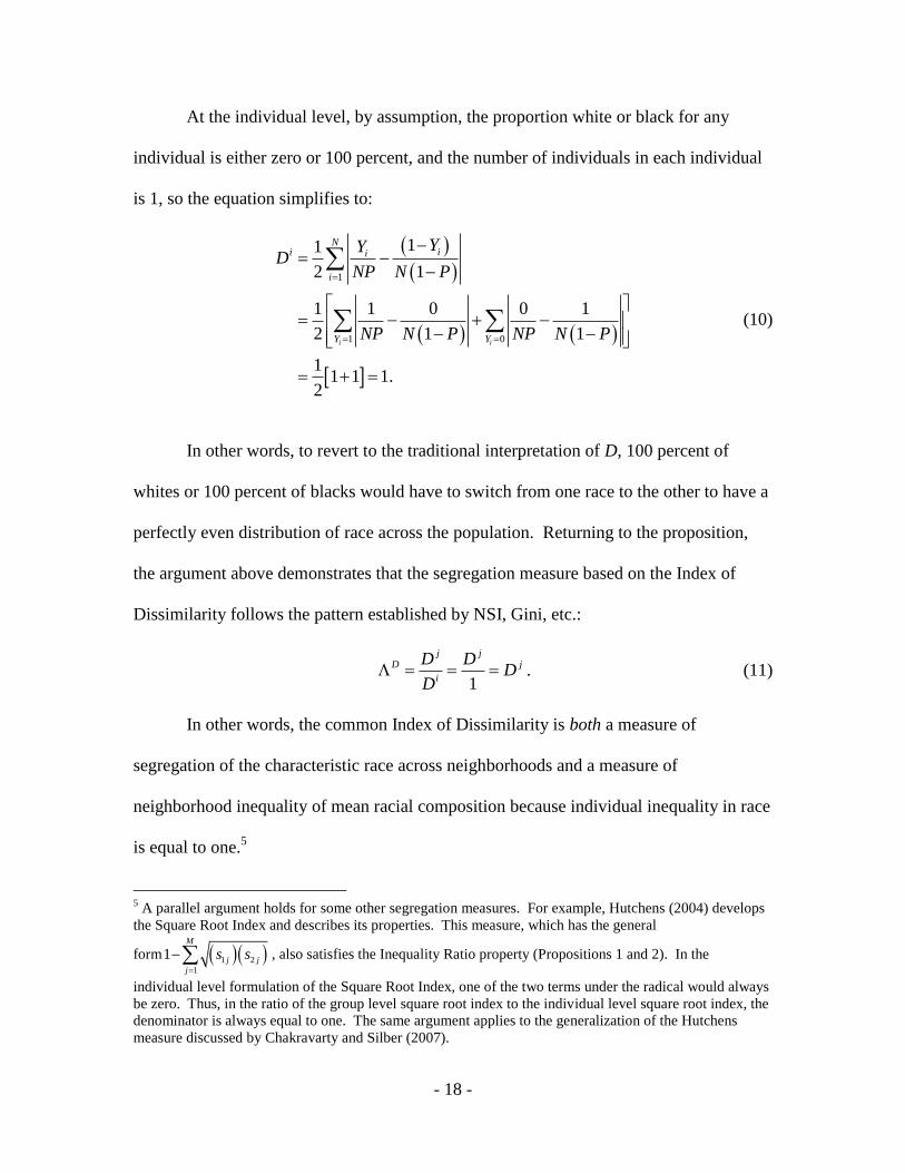
At the individual level, by assumption, the proportion white or black for any
individual is either zero or 100 percent, and the number of individuals in each individual
is 1, so the equation simplifies to:
1
1 0
11
2 1
1 1 0 0 1
2 1 1
11 1 1.
2
i i
Nii i
i
Y Y
YYD
NP N P
NP N P NP N P
(10)
In other words, to revert to the traditional interpretation of D, 100 percent of
whites or 100 percent of blacks would have to switch from one race to the other to have a
perfectly even distribution of race across the population. Returning to the proposition,
the argument above demonstrates that the segregation measure based on the Index of
Dissimilarity follows the pattern established by NSI, Gini, etc.:
1
j jD j
i
D DD
D . (11)
In other words, the common Index of Dissimilarity is both a measure of
segregation of the characteristic race across neighborhoods and a measure of
neighborhood inequality of mean racial composition because individual inequality in race
is equal to one.5
5 A parallel argument holds for some other segregation measures. For example, Hutchens (2004) develops
the Square Root Index and describes its properties. This measure, which has the general
form 1 2
1
1M
j j
j
s s
, also satisfies the Inequality Ratio property (Propositions 1 and 2). In the
individual level formulation of the Square Root Index, one of the two terms under the radical would always
be zero. Thus, in the ratio of the group level square root index to the individual level square root index, the
denominator is always equal to one. The same argument applies to the generalization of the Hutchens
measure discussed by Chakravarty and Silber (2007).

- 19 -
Extension of Dissimilarity to Multi-Race Individuals
iD is equal to one, as argued in the previous section, but only because researchers
typically characterize all persons as one group or another. For example, many studies
employing D examine white vs. non-white, or examine white vs. black ignoring all
others. It does not need to be so. In a situation where a significant number of persons are
mixed race, the standard dissimilarity measure fails to reflect reality. Armed with an
understanding of the nature of segregation as a ratio of inequality measures, we can easily
incorporate mixed-race persons. Define Yi as the proportion black for each person. Most
persons would be zero or one, but others could be 0.5, 0.25, 0.125 or any value between 0
and 1. Then the Non-Exclusive Index of Dissimilarity (NED) is:
1 1
11
1
1
1
1
M Mj jj j
j jjj jNED
Ni Nii
i
ii
nnn
N NNED
NED YY YN N
. (12)
In most racial applications in the U.S., there are probably too few persons
categorized as multiracial for this refinement to matter. However, explicit
acknowledgement of mixed-race individuals is becoming more common over time, and
the new measure could prove useful in studying ethnic and racial segregation in the
presence of mixed marriages. The NED could also be applied in contexts other than race
and ethnicity. For example, if one were examining the segregation of persons who
possessed two genetic markers, many individuals may have both genetic markers.
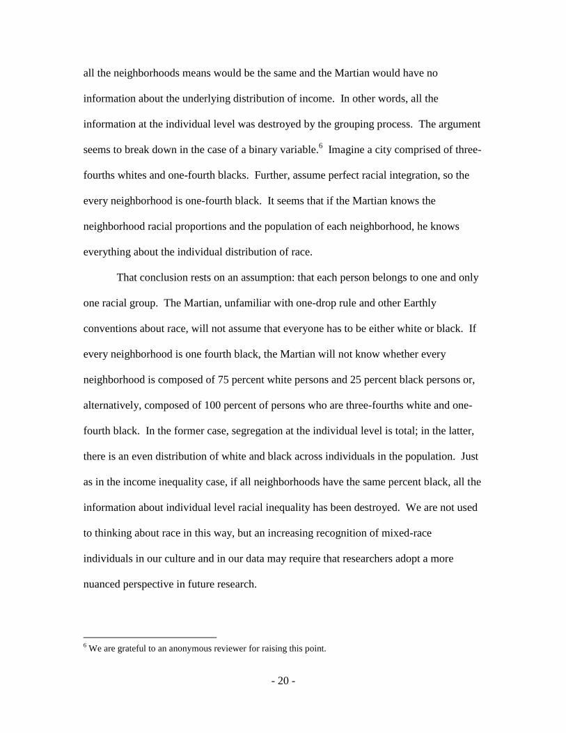
In the introduction, we discussed a Martian attempting to learn about income
inequality in a city. The Martian is given the population of the neighborhoods and the
mean income of each neighborhood. We argued that if economic segregation were zero,
- 20 -
all the neighborhoods means would be the same and the Martian would have no
information about the underlying distribution of income. In other words, all the
information at the individual level was destroyed by the grouping process. The argument
seems to break down in the case of a binary variable.6 Imagine a city comprised of three-
fourths whites and one-fourth blacks. Further, assume perfect racial integration, so the
every neighborhood is one-fourth black. It seems that if the Martian knows the
neighborhood racial proportions and the population of each neighborhood, he knows
everything about the individual distribution of race.
That conclusion rests on an assumption: that each person belongs to one and only
one racial group. The Martian, unfamiliar with one-drop rule and other Earthly
conventions about race, will not assume that everyone has to be either white or black. If
every neighborhood is one fourth black, the Martian will not know whether every
neighborhood is composed of 75 percent white persons and 25 percent black persons or,
alternatively, composed of 100 percent of persons who are three-fourths white and one-
fourth black. In the former case, segregation at the individual level is total; in the latter,
there is an even distribution of white and black across individuals in the population. Just
as in the income inequality case, if all neighborhoods have the same percent black, all the
information about individual level racial inequality has been destroyed. We are not used
to thinking about race in this way, but an increasing recognition of mixed-race
individuals in our culture and in our data may require that researchers adopt a more
nuanced perspective in future research.
6 We are grateful to an anonymous reviewer for raising this point.
- 21 -
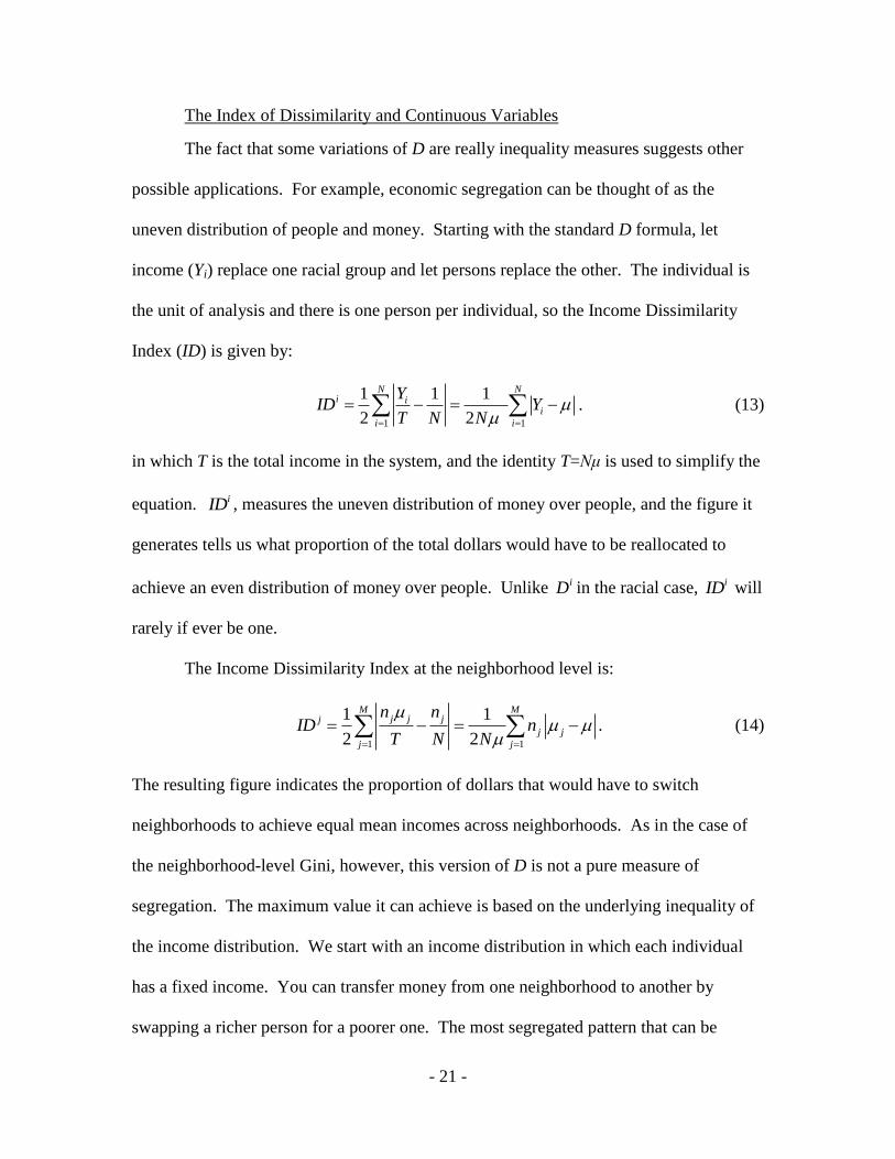
The Index of Dissimilarity and Continuous Variables
The fact that some variations of D are really inequality measures suggests other
possible applications. For example, economic segregation can be thought of as the
uneven distribution of people and money. Starting with the standard D formula, let
income (Yi) replace one racial group and let persons replace the other. The individual is
the unit of analysis and there is one person per individual, so the Income Dissimilarity
Index (ID) is given by:
1 1
1 1 1
2 2
N Ni i
i
i i
YID Y
T N N
. (13)
in which T is the total income in the system, and the identity T=Nμ is used to simplify the
equation. iID , measures the uneven distribution of money over people, and the figure it
generates tells us what proportion of the total dollars would have to be reallocated to
achieve an even distribution of money over people. Unlike iD in the racial case, iID will
rarely if ever be one.
The Income Dissimilarity Index at the neighborhood level is:
1 1
1 1
2 2
M Mj j jj
j j
j j
n nID n
T N N
. (14)
The resulting figure indicates the proportion of dollars that would have to switch
neighborhoods to achieve equal mean incomes across neighborhoods. As in the case of
the neighborhood-level Gini, however, this version of D is not a pure measure of
segregation. The maximum value it can achieve is based on the underlying inequality of
the income distribution. We start with an income distribution in which each individual
has a fixed income. You can transfer money from one neighborhood to another by
swapping a richer person for a poorer one. The most segregated pattern that can be

- 22 -
achieved is limited by the inequality at the individual level, so that if one person has all
the money and lives alone, we achieve a near total segregation of people and money. If
everyone has nearly identical incomes, even the most segregated arrangement of people
still results in a fairly even distribution of people and money across neighborhoods.
The creation of a measure of economic segregation based on the Index of Income
Dissimilarity is achieved as usual by dividing the group-level inequality by the
corresponding individual-level inequality:
1
1
M
j jjjID
Ni
i
i
nID
IDY
. (15)
The formula is identical the NED above, but the meaning of Yi is different. In the non-
exclusive case, Yi varies between zero and one, whereas for ID, Yi is the continuous
variable income. The meanings of μ and μj vary accordingly. ID looks very similar to
the square of the Neighborhood Sorting Index (Jargowsky, 1996):
2
12
2
1i
M
j j
j
N
i
n
NSI
Y
. (16)
However, in the absence of individual-level data, the ID measure is likely to be less
sensitive to assumptions that have to be made about the distribution of incomes in the
highest income bracket to estimate the parameters of the individual income distribution
(Jargowsky, 1996).

- 23 -
The Entropy Index of Segregation (H)
Shannon (1948) borrowed the entropy score from thermodynamics, and applied it
as a measure of the information content or diversity of a source. Theil and Finezza
(1971; see also Theil, 1972) adapted entropy to the measure of segregation in school
systems, defining the Entropy Index as the weighted average difference between the
entropy of schools to the overall entropy of the school system divided by the overall
entropy. The measure has been described, again in the education context, as “a measure
of how diverse individual schools are, on average, compared with the diversity of their
metropolitan area school enrollment as a whole” (Reardon et al., 2000: 353). Given the
prevalence and desirable properties of this measure, an important test of the Information
Theory of Segregation is whether H satisfies the Inequality Ratio property, as required by
Proposition 2.
The most common application of H is distinct racial groups, with the number of
groups given by r = 1 to R. Diversity in the population is measured by Shannon’s
Entropy score:
1
lnR
r r
r
E p p
, (17)
in which pr is the proportion of that category r in the overall population. A
corresponding Entropy score Ej is calculated for each group j:
1
lnR
j jr jr
r
E p p
. (18)
If there is complete integration, every group has an exactly proportional share of
each racial group, then Ej is equal to E for each group j. In a case of maximal
segregation, pjr is 1 for one category r and zero for all other r for all j; hence, Ej is zero

- 24 -
for all j. Moreover, the weighted average of the diversity of the groups can never exceed
the diversity of the population; because, as Shannon showed, the grouping process cannot
create more information than exists in the population. Thus, the weighted average group
entropy is divided by E to create a variable with a maximum of 1:
1 1
M Mj
i j i
j j
nE E n E E
NH
E NE
. (19)
Written in this form, H does not seem to satisfy the Inequality Ratio property.
In fact, H does have the structure of a ratio of inequality at the group level to
inequality at the individual level. To see this, let E represent the diversity in the
population, and let iE and jE represent the diversity of individuals and groups
respectively. Then, the inequality in diversity at the group level is the weighted mean of
jE E and the inequality in diversity at the individual level is the mean of the
expression iE E . From Proposition 2, the Entropy Index of Segregation must have
the form:
1 1
1 1
1
M Mj
j j jjj jH
N Ni
i i
i i
nE E n E E
NH
HE E E E
N
. (20)
Each individual, at least in applications of H to date, is categorized in one and
only one category of the nominal variable Y, so the diversity of any given individual is
zero. In such cases, we can simplify the expression:

- 25 -
1 1 1
1
0
M M M
j j j j j jjj j jH
Ni
i
n E E n E E n E EH
HH NE NE
E
, (21)
proving that the formulation based on Proposition 2 is equivalent to one in common use.7
H is therefore a special case of a broader measure, H , that could easily
incorporate mixed race persons or other categorizations that allow one individual to
belong to multiple groups. In the presence of mixed race (multi-category) persons, Ei
would not equal zero in all cases and the more general version of the formula would need
to be applied. Letting pir represent the proportion of each person that is category r, we
define the Non-Exclusive Entropy Index of Segregation (NEH) as:
1 1 1
1 1 1
ln ln
ln ln
M M R
j j j jr jr r rjj j rNEH
Ni N R
i ir ir r ri i r
n E E n p p p pNEH
NEHE E p p p p
. (22)
It is also interesting to note the similarity of form between this expression and the other
measures. Of course, in the usual case where individuals are assigned to one and only
one category, the first term in the denominator is either 1 ln 1 0 or 0 ln 0 that is
typically defined to be zero in segregation studies (Reardon et al., 2000).
A related point is that the Theil Inequality measure often applied to income data
(Theil, 1972), can also form an income segregation measure. By Proposition 1, if Yi is
income, we can form the Theil Income Segregation (TI) measure as follows:
7 Since the normalization by E produces a measure consistent with the Inequality Ratio Property, measures
that fail to normalize by E are not pure measures of segregation as that concept is defined in this paper. An
example is Mutual Information Index (Mora and Castillo, 2007), which combines information about sorting
with information about the overall community diversity.

- 26 -
1
1
ln
ln
Mj j
jjjTI
i N
i i
i
nTI
TI Y Y
. (23)
This measure has not been identified previously, but follows naturally from the
Information Theory of Segregation. Like the measures discussed previously, the Theil
measure can therefore be used to measure segregation with respect to binary,
polytomous, and continuous variables.
The Exposure Index
The Exposure Index, also known as the Interaction Index (I), is often described as
an alternative to the Index of Dissimilarity (D) as a measure of segregation (Bell, 1954;
Lieberson and Carter, 1982; Schnare, 1980; Zoloth, 1976). Unlike D, the Exposure Index
is asymmetric and is sensitive to the underlying population proportion, which can be
viewed as an advantage or a disadvantage (White, 1986). On the one hand, many have
argued that composition invariance is a desirable property of a segregation measure
(James and Taeuber, 1985). On the other hand, I reflects actual differences in the
probability of residential contact between two groups (Lieberson and Carter, 1982).
Assume a simple, two group situation. Let W equal total whites in the
metropolitan area, let B be the total blacks. N is the total population. Respectively, wj, bj,
and nj are the corresponding parcel figures for neighborhood j. Then, the white exposure
to blacks and the black exposure to whites are given by:
- 27 -
1
1
,
.
Mj j
w b
j j
Mj j
b w
j j
w bI
W n
b wI
B n
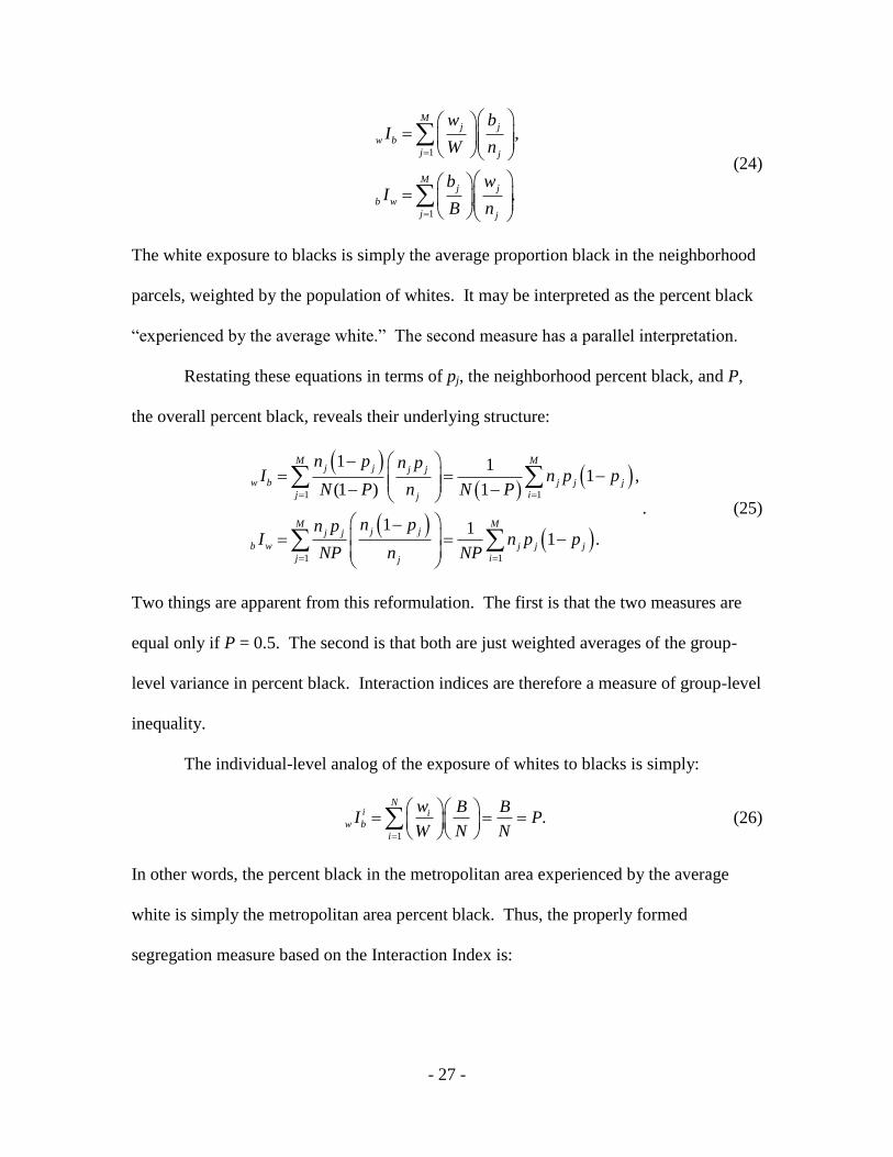
(24)
The white exposure to blacks is simply the average proportion black in the neighborhood
parcels, weighted by the population of whites. It may be interpreted as the percent black
“experienced by the average white.” The second measure has a parallel interpretation.
Restating these equations in terms of pj, the neighborhood percent black, and P,
the overall percent black, reveals their underlying structure:
1 1
1 1
1 11 ,
(1 ) 1
1 11 .
M Mj j j j
w b j j j
j ij
M Mj jj j
b w j j j
j ij
n p n pI n p p
N P n N P
n pn pI n p p
NP n NP
. (25)
Two things are apparent from this reformulation. The first is that the two measures are
equal only if P = 0.5. The second is that both are just weighted averages of the group-
level variance in percent black. Interaction indices are therefore a measure of group-level
inequality.
The individual-level analog of the exposure of whites to blacks is simply:
1
.N
i iw b
i
w B BI P
W N N
(26)
In other words, the percent black in the metropolitan area experienced by the average
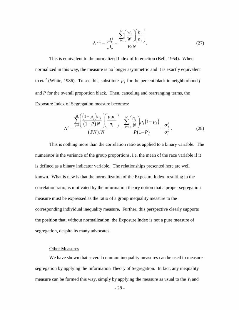
white is simply the metropolitan area percent black. Thus, the properly formed
segregation measure based on the Interaction Index is:
- 28 -
1
w b
Mj j
jj jI w b
i
w b
w b
W nI
I B N
. (27)
This is equivalent to the normalized Index of Interaction (Bell, 1954). When
normalized in this way, the measure is no longer asymmetric and it is exactly equivalent
to eta2 (White, 1986). To see this, substitute jp for the percent black in neighborhood j
and P for the overall proportion black. Then, canceling and rearranging terms, the
Exposure Index of Segregation measure becomes:
21
1
2
11
1
1
MMj j j j
j
j jj j j jI
i
p n p n np p
P N n N
PN N P P
. (28)
This is nothing more than the correlation ratio as applied to a binary variable. The
numerator is the variance of the group proportions, i.e. the mean of the race variable if it
is defined as a binary indicator variable. The relationships presented here are well
known. What is new is that the normalization of the Exposure Index, resulting in the
correlation ratio, is motivated by the information theory notion that a proper segregation
measure must be expressed as the ratio of a group inequality measure to the
corresponding individual inequality measure. Further, this perspective clearly supports
the position that, without normalization, the Exposure Index is not a pure measure of
segregation, despite its many advocates.
Other Measures
We have shown that several common inequality measures can be used to measure
segregation by applying the Information Theory of Segregation. In fact, any inequality
measure can be formed this way, simply by applying the measure as usual to the Yi and

- 29 -
then applying the measure to the Yj. For example, the Atkinson family of inequality
measures will produce a corresponding family of Atkinson Segregation measures (AS):
11 1
1
11 1
1
11
11
Mj
j jA
i
Ni
i
Y
MA
AY
N
, (29)
in which ε is the inequality aversion parameter, and can be used by researchers to make
the measure more sensitive to segregation at different levels of the income distribution.
There is an Atkinson segregation statistic that has been described for the binary case, but
it has seldom been used (James and Taeuber, 1985; White, 1986). For a binary variable,
regardless of the shape parameter ε, the individual level Atkinson inequality measure is 1.
So, once again, the binary variable formula is shown to be a special case of the
continuous variable case and the Atkinson segregation statistic is equally applicable to
binary and continuous variables.
Segregation measures based on percentile ranks are possible as well. For example
the, the Interquartile Segregation (IQS) measure is:
3 1
3 1
j jjIQR
i i i
Q QIQR
IQR Q Q
. (30)
While this measure would be insensitive to income extremes, it has the virtue of being
very easy calculate; often researchers may have group data but only summary statistics
on the individual level data, including the quartiles. Of course, any available quantiles
could be used, such as the 90th
and 10th
percentile. Clearly, the number of measures of
segregation can be greatly expanded by understanding the structural relationship between
inequality and segregation. The choice between these measures should be based on their

- 30 -
properties, judgments about the implicit weighting, and the data demands of each
measure in relation to the available data.
It is worth noting that a number of segregation measures that have been proposed
may not possess the Inequality Ratio property. Massey and Denton (1988) define five
dimensions of segregation. Two (evenness and isolation) have already been addressed in
the discussion of the Index of Dissimilarity and the Exposure Index. The other three are
spatial concentration, centralization, and clustering. These are perfectly valid and
interesting concepts, but we think that each is a hybrid measure that combines
segregation, in the sense defined here, with additional information. Echenique and Fryer
(2005) propose a Spectral Segregation Index, which aggregates information about the
social networks of members of different groups. While this may be a very desirable
measure for many purposes, from our perspective it combines information about the
sorting of individuals into groups with information about interactions between and among
members of those groups.
Theoretical vs. Structural Limts
Propositions 1 and 2 show that segregation is a measure of the information loss in
the measured level of inequality when moving from individuals to groups. Segregation is
the result of a process of allocating individual level values across spatial units. In theory,
segregation measures should vary from 1, representing no information loss, to 0,
representing total information loss. However, with a finite population these extrema may
be unachievable through sorting alone.
Shannon’s “fundamental theorem for a discrete channel with noise” is exactly on
point. It states that if a channel has a capacity C and the source has a total quantity of
- 31 -
information H, and H is greater than C, then “there exists a coding scheme such that the
output of the source can be transmitted over the channel with an arbitrarily small
frequency of errors.” This is true even on a noisy channel with random errors, a fact that
makes modern communications possible. However, “there is no method of encoding
which gives an equivocation less than H – C” (1948: 23). In the case of segregation, the
channel through which the information about the underlying individual inequality is
transmitted is the grouping structure, which in effect limits the information that can be
transmitted.
Examples will clarify the point. If the variable Y is income, and if the number of
unique values of income is greater than the number of groups M, then there is no possible
way to allocate individuals to groups without the destruction of information from the
individual level, even if individuals are assigned to groups explicitly by income rank. At
least two distinct incomes will have to be averaged within one group, losing information.
Thus, j i and will be less than one solely for structural reasons, because of the
choice of the number of parcels.
One might think that this is a problem only with continuous variables, but it can
happen for binary variables as well. Suppose there are seven whites and seven blacks in
a city with two neighborhoods. In theory, perfect segregation could be produced.
However, every household must live in a housing unit, which are durable and fixed in the
short run. If one neighborhood has 8 housing units and the other has 6, there is no way to
achieve perfect segregation. Again, the maximum level of neighborhood inequality will
fall short of the individual inequality for reasons other than sorting of units.
- 32 -
The minimum level of neighborhood inequality may fall short of zero. The
clearest example is the “Bill Gates problem.” If Bill Gates is one of the members of the
population in question, there is no way to create neighborhoods with equivalent mean
incomes. Whichever neighborhood contains Bill Gates and his money will be far richer
than any other neighborhood. One could achieve neighborhood equality only by
redistributing his income. While that might be a good idea for a variety reasons, it is not
a sorting process and it would change the underlying income distribution. In the binary
context, with fixed housing stock, neighborhoods with even numbers of housing units
cannot be made to have identical proportions with neighborhoods with odd numbers of
housing units.
As a result of these considerations, two different metropolitan areas (or the same
metropolitan area at two different points in time), both of which have been segregated to
the maximum possible extent given Yi and nj may differ in how close the measured level
of neighborhood inequality may approach the individual level of inequality.
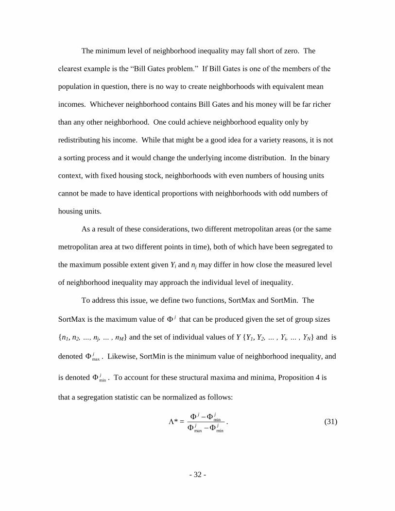
To address this issue, we define two functions, SortMax and SortMin. The
SortMax is the maximum value of j that can be produced given the set of group sizes
{n1, n2, …, nj, … , nM} and the set of individual values of Y {Y1, Y2, … , Yi, … , YN} and is
denoted max
j . Likewise, SortMin is the minimum value of neighborhood inequality, and
is denoted min
j . To account for these structural maxima and minima, Proposition 4 is
that a segregation statistic can be normalized as follows:
min
max min
* = j j
j j
. (31)
- 33 -
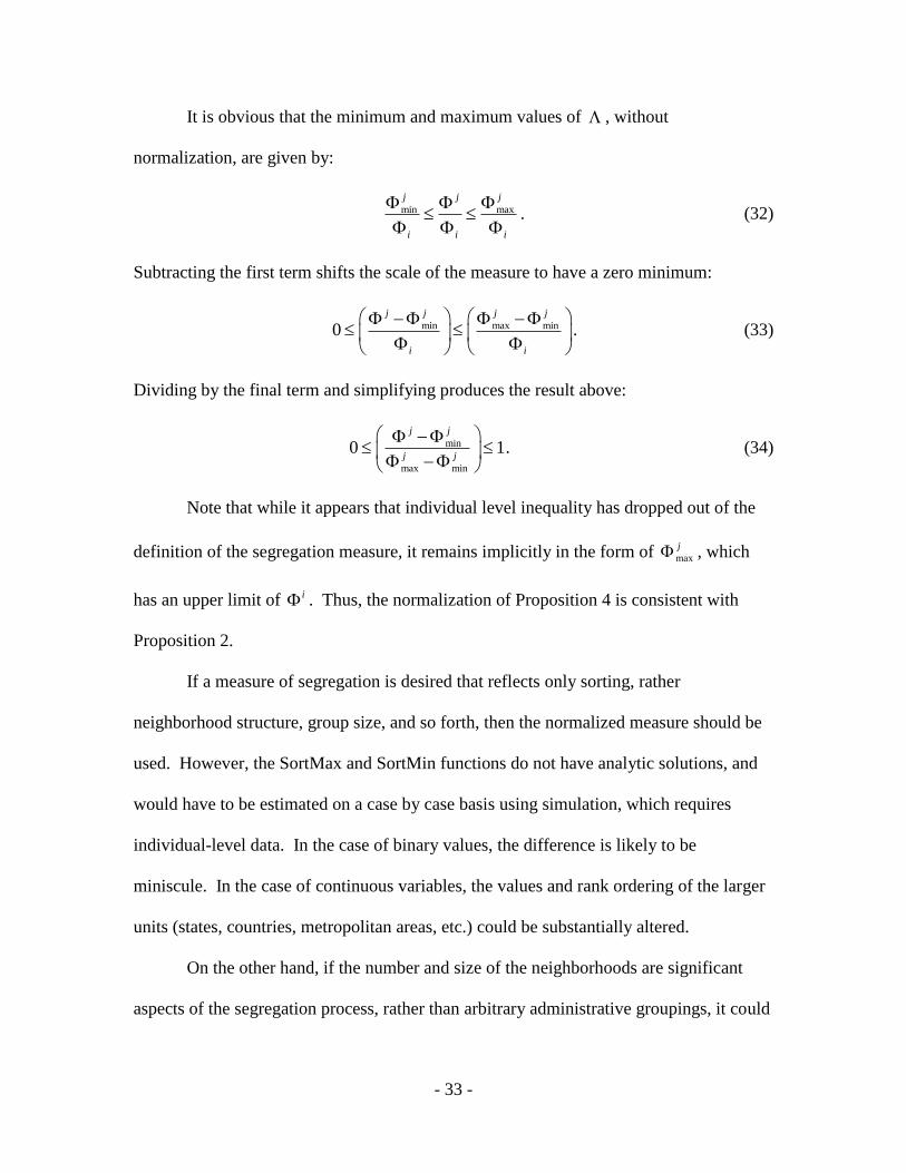
It is obvious that the minimum and maximum values of , without
normalization, are given by:
min max
j j j
i i i
. (32)
Subtracting the first term shifts the scale of the measure to have a zero minimum:
min max min0j j j j
i i
. (33)
Dividing by the final term and simplifying produces the result above:
min
max min
0 1j j
j j
. (34)
Note that while it appears that individual level inequality has dropped out of the
definition of the segregation measure, it remains implicitly in the form of max
j , which
has an upper limit of i . Thus, the normalization of Proposition 4 is consistent with
Proposition 2.
If a measure of segregation is desired that reflects only sorting, rather
neighborhood structure, group size, and so forth, then the normalized measure should be
used. However, the SortMax and SortMin functions do not have analytic solutions, and
would have to be estimated on a case by case basis using simulation, which requires
individual-level data. In the case of binary values, the difference is likely to be
miniscule. In the case of continuous variables, the values and rank ordering of the larger
units (states, countries, metropolitan areas, etc.) could be substantially altered.
On the other hand, if the number and size of the neighborhoods are significant
aspects of the segregation process, rather than arbitrary administrative groupings, it could
- 34 -
be argued that the un-normalized measure is both descriptively and substantively
accurate.
Conclusion
We argue that segregation is fundamentally analogous to the loss of information
from an aggregation process. Integration is information loss and segregation is
information retention. In the case of signal processing, compression of graphics files, or
the estimation of income distribution parameters from grouped data, the question is how
to minimize information loss. In the case of segregation, the question is how much
information about the underlying distribution remains after the population is sorted in
groups, particularly geographic neighborhoods. While these questions have different
motivations, they have the same mathematical structure.
We argued that the information theory framework requires that a segregation
measure must be structured as the ratio of an inequality measure applied to the group data
to the same inequality measure applied to the individuals in the population. Of course,
any researcher is free to invent any measure and call it segregation. In particular
situations, a nonconforming measure may prove useful. However, we suspect that any
such measure will not be a pure segregation measure, just as the neighborhood-level Gini
reflected both sorting and underlying inequality. Ultimately, what constitutes a
segregation measure is a conceptual question, not a mathematical one. Our position is
normative in that we think the logic of the information theory analogy is so strong that all
researchers should adopt it. (Most have implicitly done so already, by using measures of
segregation that are consistent with the framework.)

- 35 -
With any theoretical formulation, the test of its value is the extent to which it
unites diverse phenomena and proves useful in understanding and resolving problems
within a field. A reexamination of a number of segregation and inequality measures in
light of the framework revealed several interesting points and useful applications. First,
some measures that have been used to measure segregation, like the neighborhood-level
Gini and the Exposure Index, are not proper segregation measures at all. In fact, they are
neighborhood inequality measures.
Second, all the standard measures of segregation can handle binary or continuous
variables. The distinction between these two types of measures is largely artificial. The
binary formulas in use were correct because the denominator of the correctly specified
segregation measure is one. Based on Proposition 2, the correct denominator for the
continuous case is easy to specify. We presented several new measures using this
approach, such as the Gini Segregation Index (GS) and Income Dissimilarity (ID).
Third, the requirement for non-overlapping groups in segregation studies is shown
to be an artificial limitation that was a function of not understanding the implicit
denominator of the Index of Dissimilarity and related measures. We presented two new
measures, the Non-Exclusive Index of Dissimilarity (NED) and the Non-Exclusive
Entropy Index of Segregation (NEH) that can easily accommodate mixed-race individuals
in a segregation analysis.
Fourth, although the formulas and means of calculation for a number of
segregation measures look quite different in their standard forms, they can all be recast in
a common mathematical structure. As Firebaugh (1999) observed with respect to
- 36 -
inequality measures, measures of segregation differ primarily in the functional form used
to aggregate individual or group differences from the overall mean.
Fifth, the lower and upper bounds of a segregation measure are theoretically zero
and one, but with finite groups of fixed size and a given finite distribution of the outcome
of interest, the actual bounds will often fall short of those values. Comparisons among
different cities or school systems could well be affected by these considerations. A
normalization is proposed that provides a pure measure of segregation unaffected by
structural limitations.

i
References
Bell, Wendell. 1954. "A probability model for the measurement of ecological
segregation." Social Forces 32:357-364.
Brown, M. C. 1994. "Using Gini-Style Indexes to Evaluate the Spatial Patterns of Health
Practitioners: Theoretical Considerations and an Application Based on Alberta
Data." Social Science & Medicine 38:1243-1256.
Duncan, Otis Dudley and Beverly Duncan. 1955. "A methodological analysis of
segregation indexes." American Sociological Review 20:210-217.
Echenique, Federico and Roland G. Fryer, Jr. 2005. “On the Measurement of
Segregation.” Unpublished paper.
Farley, Reynolds. 1977. "Residential segregation in urbanized areas of the United States
in 1970: an analysis of social class and racial differences." Demography 14:497-
517.
Firebaugh, G. 1999. "Empirics of world income inequality." American Journal of
Sociology 104:1597-1630.
Gini, Corrado. 1912. “Variabilita e mutabilita.” Reprinted in E. Pizetti and T.
Salvemini, eds., Memorie di Metodologia Statistica. Rome: Libreria Erendi
Virgilio Veschi, 1955.
_____. 1921. “Measurement of Inequality of Incomes.” The Economic Journal.
31:124-126.
Hardman, A. and Y. M. Ioannides. 2004. "Neighbors' income distribution: economic
segregation and mixing in US urban neighborhoods." Journal of Housing
Economics 13:368-382.
Hutchens, R. 2001. "Numerical measures of segregation: desirable properties and their
implications." Mathematical Social Sciences 42:13-29.
Hutchens, R. 2004. "One measure of segregation." International Economic Review
45:555-578.
Ioannides, Y. M. 2004. "Neighborhood income distributions." Journal of Urban
Economics 56:435-457.
Jahn, J., Schmid, C. F. & Schrag, C. 1947. “The measurement of ecological
segregation.” American Sociological Review 3:293-303.

ii
James, Franklin J. 1986. "A new generalized 'exposure-based' segregation index:
demonstration in Houston and Denver." Sociological Methods and Research
14:301-316.
James, D. R. and K. E. Taeuber. 1985. "Measures of Segregation." Sociological
Methodology 15:1-32.
Jargowsky, Paul A. 1996. "Take the money and run: economic segregation in U.S.
metropolitan areas." American Sociological Review 61:984-998.
Kim, Jeongdai and Paul A. Jargowsky. 2005. “The Gini Coefficient and Segregation
along a Continuous Dimension.” National Poverty Center Working Paper Series,
No. 02-05. Gerald R. Ford School of Public Policy, University of Michigan.
Lieberson, Stanley and Donna K. Carter. 1982. "Temporal changes and urban differences
in residential segregation: a reconsideration." American Journal of Sociology
88:296-311.
Massey, Douglas S. and Nancy A. Denton. 1988. "The dimensions of racial segregation."
Social Forces 67:281-315.
Massey, Douglas S. and Mitchell L. Eggers. 1990. "The ecology of inequality: minorities
and the concentration of poverty, 1970-1980." American Journal of Sociology
95:1153-1188.
Milanovic, B. 2002. "True world income distribution, 1988 and 1993: First calculation
based on household surveys alone." Economic Journal 112:51-92.
Morgan, B. S. 1975. "Segregation of Socio-Economic Groups in Urban Areas: A
Comparative Analysis." Urban Studies 12:47-60.
Mora, Ricardo and Javier Ruiz-Castillo. 2007. “The Statistical Properties of the Mutual
Information Index of Multigroup Segregation.” Working Paper 07-74, Economic
Series 43, Universidad Carlos III de Madrid.
Pyatt, G. 1976. “On the interpretation and disaggregation of Gini coefficients.”
Economics Journal 86:243-255.
Reardon, S. F. and G. Firebaugh. 2002. "Measures of multigroup segregation."
Sociological Methodology 2002, Vol 32 32:33-67.
Reardon, S. F., J. T. Yun, and T. M. Eitle. 2000. "The changing structure of school
segregation: Measurement and evidence of multiracial metropolitan-area school
segregation, 1989-1995." Demography 37:351-364.
Sakoda, J. M. 1981. "A generalized index of dissimilarity." Demography 18:245-250.

iii
Schnare, Ann B. 1980. "Trends in residential segregation by race: 1960-1970." Journal of
Urban Economics 7:293-301.
Schwartz, W. B., J. P. Newhouse, B. W. Bennett, and A. P. Williams. 1980. "The
Changing Geographic Distribution of Board-Certified Physicians." New England
Journal of Medicine 303:1032-1038.
Shannon, C. E. 1948. "A Mathematical Theory of Communication." Bell System
Technical Journal 27:379-423, 623-656.
Silber, J. 1989. "Factor Components, Population Subgroups and the Computation of the
Gini Index of Inequality." Review of Economics and Statistics 71:107-115.
Theil, Henri. 1972. Statistical Decomposition Analysis. Amsterdam: North Holland.
Theil, H. and A. J. Finizza. 1971. "Note on Measurement of Racial Integration of Schools
by Means of Informational Concepts." Journal of Mathematical Sociology 1:187-
193.
White, Michael J. 1986. "Segregation and diversity measures in population distribution."
Population Index 52:198-221.
Winship, Christopher. 1977. "A revaluation of indexes of residential segregation." Social
Forces 55:1058-1066.
Yao, S. 1999. “On the decomposition of Gini coefficients by population class and
income source: a spreadsheet approach and application.” Applied Economics
31:1249-1264.
Zoloth, Barbara S. 1976. "Alternative measures of school segregation." Land Economics
52:278-293.
Top Related