


Languages
Pages
Legal

Sequential data assimilation of the 1D Hawkes Process for urban
crime data
Naratip Santitissadeekorn1, Martin B. Short2, and David J.B. Lloyd1
1Department of Mathematics, University of Surrey, Guildford, GU2 7XH, UK2Georgia Tech Mathematics Department, Atlanta, GA, USA
October 25, 2017
Abstract
The self-exciting crime rate model known as the Hawkes process is the basis for some recently
developed predictive policing algorithms. Model parameters are often found using maximum
likelihood estimation (MLE), but this approach has several limitations. As an alternative, we
develop here a novel Bayesian sequential data assimilation algorithm for joint state-parameter
estimation by deriving an approximating Poisson-Gamma ‘Kalman’ filter, that allows for un-
certainty quantification for inhomogeneous Poisson data. The ensemble-based implementation
of the filter is developed in a similar approach to the ensemble Kalman filtering making the
filter applicable to large-scale real world applications unlike nonlinear filters such as the particle
filter. We demonstrate the filter on synthetic and real Los Angles gang crime data and compare
it against the “gold-standard” particle filter showing its effectiveness in practice. We investigate
the predictability of the Hawkes process using the Receiver Operating Characteristic (ROC) to
provide a useful indicator for when predictive policing software for a crime type is likely to be
useful. We also use the ROC to compare forecast skill of sequential data assimilation and MLE.
We find that sequential data assimilation produces improved forecasts over the MLE for the
gang crime data.
1 Introduction
Constructing computational algorithms for predictive policing is one of the emerging areas of math-
ematical research. Given that police departments worldwide are frequently asked to deliver better
service with the same level of resources, algorithms that can better allow authorities to focus their
resources could be of great value. To this end, there have been several methods developed over the
years to help make crime predictions and ultimately guide policing resources to areas where they
are likely to have the biggest impact.
One recently developed algorithm for predictive policing is the Epidemic-Type-Aftershock-Sequences
(ETAS) model described in some detail in [19, 20]. The idea behind the ETAS model is that crimes
are generated stochastically, but the rate of crime generation is history-dependent, such that crimes
occurring within an area will increase the rate of future crime generation in that same or nearby
areas for at least some period of time. In practice, the ETAS model functions by taking in daily,
up-to-date historical crime data in the form of event times and geolocations, processing them within
1

the model’s mathematical framework described below, and then highlighting on a fixed grid (typi-
cally 150m squares) the top N locations likely to have crime on that day. The processing is done
by carrying out a time series analysis in each grid cell by fitting a self-exciting rate model known
as a Hawkes process to the historical data. The stochastic event rate λ(t) in this Hawkes process
is given by
λ(t) = µ+∑τj<t
qβe−β(t−τj), (1.1)
where µ is the baseline crime rate, q is a sort of reproduction number that is equal to the expected
number of future events spawned by any single crime occurrence, β is the decay rate of the increased
crime rate back to the baseline, and τj are the times of prior crime events. Hence, at any given
moment the crime rate is a linear superposition of Poisson processes, including the homogeneous
baseline rate and several exponentially decaying rates equal in number to the number of prior
events. The ETAS algorithm then carries out a maximum likelihood parameter estimation (MLE)
to find µ, θ, and β; typically θ and β are assumed to be the same across all grid cells, while µ is
allowed to vary from cell to cell. Finally, those N cells with the highest estimated λ are highlighted
for that day.
Two recent randomised field-trials conducted with police departments in Los Angles, CA and Kent,
UK [20] showed that the ETAS algorithm was able to predict 1.4-2.2 times as much crime as a
dedicated crime analyst using existing criminal intelligence and hotspot mapping practices. The
trials were also able to show that dynamic police patrolling based on the ETAS algorithm led to an
average of 7.4% reduction in crime volume at mean weekly directed patrol levels, whereas patrols
based upon analyst predictions showed no statistically significant effect.
Despite the success of these field-trials, one fundamental question for any predictive policing al-
gorithm is whether or not a given crime type is ‘predictable’ at any practical level, and by how
much. Analysing the operational predictability and forecast skill of any predictive policing software
is crucial in determining its worth. That is, even if one had a perfect model for the crime rate and
complete knowledge of all model parameters, would the resulting predictions be actionable in any
useful way? Currently, there has been no assessment from a basic level of when crime location and
rate is fundamentally predictable (or not), despite the fact that this knowledge would be useful for
both police forces and predictive policing researchers and companies.
Another problem with current techniques is that they typically have no ability to track uncertainty
in either the fitted parameters or the model predictions, which could arise due to noisy and limited
data or model selection errors. While forecasts such as the ETAS cell highlighting would not
necessarily take into account such uncertainty, it is important to know from a patrolling strategy
perspective. For instance, measures of uncertainty can help to determine if the police are more
likely to cover the most crime locations by increasing/decreasing the number of locations to patrol.
In order to overcome some of these problems and fill in gaps within the literature, we propose
here a sequential data assimilation approach to predictive policing that will systematically incor-
porate uncertainty and real-time tracking, enabling us to investigate the effect of uncertainty in
an operational context. To do this in a computationally efficient manner, we develop an Ensem-
ble Poisson-Gamma filter motivated by the Ensemble Kalman Filter (EnKF) used in geophysical
applications [6, 12]. Even though EnKF allows for non-normal prior distributions and relaxes the
assumption of a normal likelihood, a highly skewed and non-negative (posterior) distribution can
2

be better approximated, for instance, by a gamma distribution. The uncertainty of crime intensity
rate and observations for some type of crimes (e.g. burglary) could be small, leading to a highly
skewed uncertainty for the burglary rate. By taking the EnKF philosophy we build a computation-
ally efficient and robust filter for the Hawkes process that compares well with the “gold-standard”
particle filter that is implemented in a large sample size limit. We note that while we are able to
use the gold-standard particle filter for a single 1D Hawkes process, in practice predictive policing
software (such as PredPol) has to carry out filtering for many grid cells making it computationally
infeasible.
We also assess the operational predictability and forecasting skills of Poisson rate models at a
fundamental level using the Receiver Operating Characteristic (ROC). This characteristic measures
the positive hit rate verses the false alarm rate and allows us to assess predictive policing models
precisely. The ROC has been suggested before by a few authors (e.g. [14]) as a good way to
measure the success or failure of predictive policing software; however their studies have focused on
particular data sets rather than a theoretical assessment of parameter regions where the Hawkes
process is predictable or not. By carrying out a theoretical synthetic experiment using the particle
filter, we find parameter regions where the Hawkes process is “ROC-predictable” and where the
data assimilation approach shows improved skill over the MLE based ETAS algorithm. We further
demonstrate our method on real LA gang violence data to show its effectiveness in practice.
The paper is outlined as follows. In section 2 we introduce ensemble filtering for sequential data
assimilation, provide an overview of the “gold-standard” particle filter approach, then develop our
own approach that we call the Ensemble Poisson-Gamma filter for a univariate variable. In section
3 we demonstrate both the accuracy and efficiency of our approach versus the particle filter on
simulated data generated via a Hawkes process that also allows a joint state-parameter estimation.
In section 4 we employ our method on real data from Los Angeles and assess the results. In section
5 we undertake a general study on the inherent predictability of Poisson rate models, then compare
our method to the ETAS algorithm. Finally, we conclude and discuss future directions and open
questions in section 6.
2 Ensemble-based filtering
Consider a counting process N(t) associated with the conditional intensity function
λ(t|Ht) := limδt→0
Pr(N(t+ δt)−N(t) = 1|Ht)
δt, (2.1)
where Ht is the event history {0 < τ1 < · · · τN(t) < t}, τj is the time of the j-th count and τN(t) is
the time of the last event prior to t. For a small interval δt, we assume that the observation, called
yo, has likelihood conditional on λ(t) and is approximated by a Poisson model
Pr(yo|λ(t)) = (λ(t)δt)yo
exp(−λ(t)δt), (2.2)
where yo = N(t+ δt)−N(t), i.e., the counts between time t and t+ δt. Note that we have assumed
that δt is small enough that at most one count is observed in the interval δt (i.e. yo = 1 or yo = 0).
For this work, we consider a discrete-time with δt small enough such that the above assumption is
approximately satisfied. Let yoj be the number of count the j-th interval, all of which is assumed
3

to have the same size of δt and YN = {yok} for k = 1, . . . , N denote the collection of the data
up to the N -th count. The state of the system and model parameters during a time interval δt
are assumed to be a constant and we use vj to collectively denote both state and parameters in
the j−th time interval. One goal of this paper is to develop a discrete-time filtering method for
the intensity process described by (2.1) and (2.2) that involves a recursive approximation of the
probability density P (vj |Yj) given the probability density P (vj−1|Yj−1). In other words, we wish
to recursively make an inference of the unknown state of a dynamical system (as well as model
parameters) using only the data from the past up to the present.
The computation of P (vj |Yj) consists of two main steps: (1) Prediction step, which computes
P (vj |Yj−1) based on P (vj−1|Yj−1) using the transition kernel P (vj |vj−1); and (2) Analysis step,
which uses Bayes’s formula to compute P (vj |Yj) given a prior density P (vj |Yj−1) for vj . When
the prior density and likelihood are both normal, the normal posterior density P (vj |Yj) is given
in a closed-form expression by the Kalman filter. However, a numerical approximation is typically
needed in general cases. One such method, discussed more extensively below, is the particle filtering
(PF) method, which provides an ensemble approximation of P (vj |Yj). This method has become
increasingly popular in practical applications since it is relatively simple to implement and able
to reproduce the true posterior P (vj |Yj) in the large sample limit. Nevertheless, it suffers from
the curse of dimensionality and the design of efficient algorithms can be challenging. Though the
time-series examples considered in this work may all be tractable with the standard PF method,
our ultimate goal is to consider higher dimensional spatio-temporal data, which may require an
algorithm that is more scalable than PF. This motivates us to develop a novel ensemble-based
filtering algorithm aiming to assimilating data where the likelihood function is described by (2.2)
for the application to crime data analysis in mind. The new algorithm is built upon the Poisson-
gamma conjugate pair in the univariate case, which can be extended to a multivariate case via the
serial update scheme as commonly used in the serial-update version of the ensemble Kalman filter
(EnKF), see [2]. Unlike the PF, where particle weight is updated according to Bayes’s rule, the
new algorithm provides a formula that attempts to directly move the ensemble into the region with
a high posterior probability.
2.1 Particle filter (PF)
We present here how a basic particle filter (PF) works in a nutshell for our specific application and
encourage the reader to consult [8, 10, 13, 16, 17] for theoretical details and discussions in general
cases. The main of idea of PF is to recursively approximate P (vj−1|Yj−1) by M weighted particles
P (vj−1|Yj−1) ≈M∑i=1
w(i)j−1δ(vj−1 − v
(i)j−1),
M∑i=1
w(i)j−1 = 1.
In the prediction step, the particle approximation of P (vj |Yj−1) is simply drawn by propagating
v(i)j−1 according to a “state-space” version of the Hawkes process (1.1), which is the model (3.1) as
discussed in Section 3. The particle weight is unchanged in this step. Thus, the prediction step
yields an ensemble approximation
P (vj−1|Yj−1) ≈M∑j=1
w(i)j−1δ(vj|j−1 − v
(i)j|j−1),
4

where vj|j−1 ∼ P (vj |Yj−1).
In the analysis step, the data is assimilated to update the particle weight via Bayes’s formula. The
new particle weight is updated as
w(i)j =
w(i)j∑M
i=1 w(i)j
, w(i)j = Pr(yoj |v
(i)j )w
(i)j−1. (2.3)
This gives the ensemble approximation of P (vj |Yj) as {w(i)j , v
(i)j }. The above algorithm may lead
to the issue of weight degeneracy when only few particles have significant particle weights and all
other weights are negligibly small. In the extreme case, there could eventually be only one particle
left with weight 1. An additional step called resampling is conventionally employed to mitigate this
flaw. The implementation of the resampling step in this work is based on the residual resampling
method, see Appendix 6. Note that the above weight update is usually called the “bootstrap filter”,
which is the simplest version of PF, but it is usually considered to be inefficient since it may require
a large number of particle to well approximate the desired density, depending on many factors such
as the dynamic of the model, the likelihood function, and the dimension of the problem. A more
general weight update equation can be designed based on importance sampling and in some cases an
optimal proposal density can be achieved to minimise the variation of the sample representation.
The detail of the optimal particle filtering is out of the scope of the current work and in-depth
discussion may be found in [10, 17]. We will use the bootstrap filter in this work since we are able
to increase the sample size to the level where the ensemble distribution is unchanged as the sample
size increases. Due to its convergence property, the PF-generated ensemble, in a large sample
limit, will be used as the gold standard to test the performance of our novel ensemble method in
Section 2.2.
2.2 Poisson-Gamma filter
We now demonstrate how we develop a filtering algorithm based on the Poisson-Gamma conjugate
pair, specified through the mean and “relative variance” of the univariate random variable λ. It
will be seen later that the filtering formula will be more compact when using the relative variance
Pr = P/〈λ〉2, where 〈λ〉 is the mean of λ, instead of the variance of λ, denoted by P . Following
standard Bayesian analysis, it is simple to show that if λ has a gamma prior distribution with a
mean 〈λ〉 and “relative” variance Pr, then given the Poisson distribution on yo in 2.2, the posterior
on λ is also gamma distributed with mean and relative variance 〈λa〉 and P ar given by
〈λa〉 = 〈λ〉+〈λ〉
P−1r + 〈λ〉δt(yo − 〈λ〉δt)
(P ar )−1 = P−1r + yo.
(2.4)
Note that the conventional Bayesian scheme updates the posterior gamma distribution via the so-
called scale and shape parameters instead of mean and relative variance. The update formula (2.4)
will, however, suite well with our ensemble-based filtering algorithm that is intended to approxi-
mately sample the posterior density for a given prior ensemble; this is analogous to the well-known
Ensemble Kalman filter (EnKF) which is widely used to sample the posterior distribution when
the assumption of normality is not strictly valid but can still be approximately satisfied. In our
application, although the prior density may not be exactly a gamma distribution, which tends to
5

be the case in practice, we may still insist to update our ensemble of λ so that its mean and relative
variance satisfy (2.4). This is drastically different from fitting the gamma distribution to the en-
semble of λ and then updating the scale and shape parameters of the gamma distribution through
Bayesian analysis and finally drawing the posterior sample from the posterior gamma distribution
described by the updated scale and shape parameters. The latter will always have the sample dis-
tributed exactly as a gamma distribution while the former can have a non-gamma sample. We will
refer to (2.4) as the Poisson-Gamma filter (PGF) and its ensemble-based version as the ensemble
Poisson-Gamma filter (EnPGF), which will be derived in the subsequent section.
We now explain how we will generate a posterior sample that satisfies (2.4). Let’s suppose that we
have a prior sample λi for i = 1, . . . ,M . Let A = [λ1, . . . , λM ]− λ be the “anomaly” matrix of size
1×M , where λ is the sample mean. Thus we can write the sample variance by P = (AAT )/(M−1)
and the relative sample variance Pr can be found accordingly using the sample mean. Given (2.4),
we can easily update the posterior ensemble mean, denoted by λa, as follows:
λa = λ+λ
P−1r + λδt(y − λδt) (2.5)
The update of the posterior ensemble anomaly, denoted by Aa, is also required so that the posterior
sample can be generated by λa = λa+Aa. It is important that the anomaly Aa must be able to pro-
duce an ensemble that is consistent with the second line of (2.4). There are several ways to achieve
this, which are analogous to several ensemble-based schemes of EnKF, see [6, 15] for “stochastic”
formulations and [1, 4] for “deterministic formulations”. We focus only on the development of the
so-called stochastic formulation in the next section.
2.3 EnPGF: Stochastic update
We first note that, if yo = 0, (2.4) indicates that the ensemble mean should update, but the
ensemble relative variance should remain unchanged. In order to achieve this along with (2.5),
one can simply scale each ensemble member such that λai = λiλa/λ, and the update is complete.
But, for yo 6= 0, we use a stochastic update scheme in which each individual ensemble member is
stochastically perturbed to achieve the sample variance that satisfies (2.4). This can be achieved
based on the following stochastic equation:
λai − λaλa
=λi − λλ
+ Pr(Pr + (yo)−1)−1[yi − ¯y
¯y− λi − λ
λ
], (2.6)
where yiiid∼ Ga(yo, 1) for i = 1 . . . ,M .
The derivation of (2.6) follows a similar idea of the gamma prior and inverse gamma likelihood
filter introduced by [3]. Denote each term in (2.6) as the following:
λai − λaλa︸ ︷︷ ︸:=w
=λi − λλ︸ ︷︷ ︸:=s
+Pr(Pr + (yo)−1)−1︸ ︷︷ ︸:=c
[yi − ¯y
¯y︸ ︷︷ ︸:=t
−λi − λλ
], (2.7)
Note that E[w2] is the posterior relative variance P ar , E[s2] is the prior relative variance Pr, and
E[t2] = Var(y)/(E[y])2 = (yo)−1 since y ∼ Ga(yo, 1). It is also simple to check that E[st] = 0.
6

Then, by taking the expectation E[w2] given the equation above, it follows that
E[w2] = E[s2]− 2cE[s2] + 2c2E[s2 + t2]
P ar = Pr − 2cPr + c2(Pr + (yo)−1)
= Pr − 2Pr(Pr + (yo)−1)−1Pr + Pr(Pr + (yo)−1)−1Pr
= Pr − Pr(Pr + (yo)−1)−1Pr,
which, after some simple algebra, matches the update in (2.4). Based on the relative anomaly (2.6),
the anomaly Aa for the posterior ensemble can be readily obtained
Aa =
(λai − λaλa
)λa. (2.8)
Therefore, (2.5) and (2.6) together complete our ensemble update algorithm, which we call the
Ensemble Poisson-Gamma filter (EnPGF).
2.4 Tests: Gamma prior and mixture of gamma prior
In this section we compare the performance of EnPGF and the ensemble Kalman filter (EnKF) in
the scenarios where the analytical form of the posterior distribution is available. The sequential
aspect of the algorithm is not tested in these cases (i.e. there is just a single observation and δt = 1
in above formula). It will be shown that EnPGF outperforms EnKF in most cases, even in the case
of large observation yo. To this end, we first present a stochastic update method for the ensemble
Kalman filter (EnKF), which is a very popular method, especially in geophysical applications, for
approximation of filtered distributions in high-dimensional applications. The EnKF exploits the
mean and covariance update of the Kalman filter to sample a high probability region of the filtered
distribution in the applications where prior sample and observation likelihood are close to being
normal. For large λ, it is appealing to apply the EnKF to approximate the uncertainty of λ because
if yo ∼ Poi(λ), yo can be approximated by a normal distribution N(λ, λ). Nonetheless, we would
have to deal with the homoskedasticity issue. To get around this, we apply the variance stabiliz-
ing transformation, i.e., z =√yo + 1/4 ∼ N(
√λ, 1/4). Therefore, we may use the transformed
observation equation for EnKF:
z =√λ+ η,
where η ∼ N(0, 1/4). The standard EnKF with stochastically perturbed observation provides a
formulation to update the sample as the following:
λai = λi +Ke(√yo + 1/4 + ηi − zi),
where zi =√λi, ηi ∼ N(0, 1/4) and Ke is the (ensemble-based) Kalman gain. The discussion of
above implementation of EnKF can be found in [6]. We will show in the subsequent section that,
albeit appealing, EnKF fails to provide a correct sample representation of the true posterior even
in the case of a large λ.
In the tests below, the ensemble size is 100 for both EnPGF and EnKF.
TEST 1: We want to ensure that when the prior sample comes from a gamma distribution, the
EnPGF in (2.6) can accurately sample the correct posterior density. We test the EnPGF and
EnKF algorithms for various gamma prior densities and observations, which are chosen so that
7
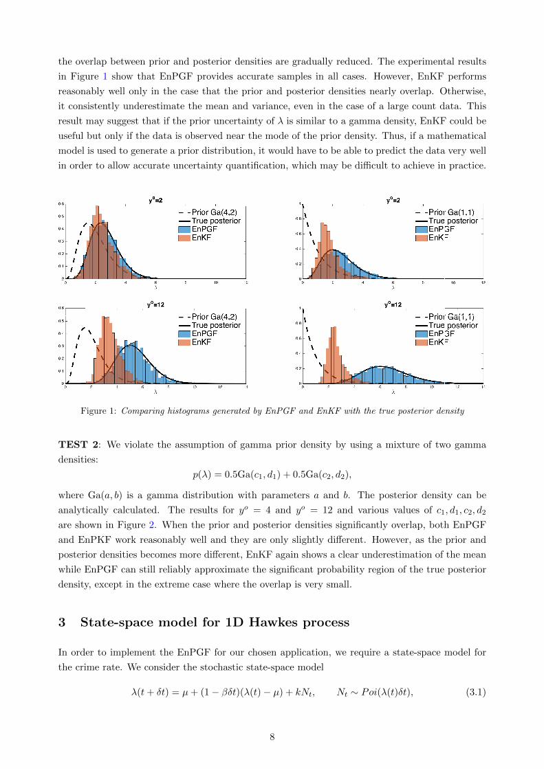
the overlap between prior and posterior densities are gradually reduced. The experimental results
in Figure 1 show that EnPGF provides accurate samples in all cases. However, EnKF performs
reasonably well only in the case that the prior and posterior densities nearly overlap. Otherwise,
it consistently underestimate the mean and variance, even in the case of a large count data. This
result may suggest that if the prior uncertainty of λ is similar to a gamma density, EnKF could be
useful but only if the data is observed near the mode of the prior density. Thus, if a mathematical
model is used to generate a prior distribution, it would have to be able to predict the data very well
in order to allow accurate uncertainty quantification, which may be difficult to achieve in practice.
Figure 1: Comparing histograms generated by EnPGF and EnKF with the true posterior density
TEST 2: We violate the assumption of gamma prior density by using a mixture of two gamma
densities:
p(λ) = 0.5Ga(c1, d1) + 0.5Ga(c2, d2),
where Ga(a, b) is a gamma distribution with parameters a and b. The posterior density can be
analytically calculated. The results for yo = 4 and yo = 12 and various values of c1, d1, c2, d2
are shown in Figure 2. When the prior and posterior densities significantly overlap, both EnPGF
and EnPKF work reasonably well and they are only slightly different. However, as the prior and
posterior densities becomes more different, EnKF again shows a clear underestimation of the mean
while EnPGF can still reliably approximate the significant probability region of the true posterior
density, except in the extreme case where the overlap is very small.
3 State-space model for 1D Hawkes process
In order to implement the EnPGF for our chosen application, we require a state-space model for
the crime rate. We consider the stochastic state-space model
λ(t+ δt) = µ+ (1− βδt)(λ(t)− µ) + kNt, Nt ∼ Poi(λ(t)δt), (3.1)
8

Figure 2: Comparing histograms generated by EnPGF and EnKF with the true posterior density for the
mixture of gamma prior densities. (Top left) yo = 4 and Prior distribution of λ is 0.5Ga(1, 1) + 0.5Ga(5, 1).
(Top right) yo = 4 and Prior distribution is 0.5Ga(1, 1) + 0.5Ga(3, 3). (Bottom left) yo = 12 and Prior
distribution is 0.5Ga(10, 1) + 0.5Ga(5, 1). (Bottom right) yo = 12 and Prior distribution is 0.5Ga(1, 1) +
0.5Ga(5, 1).
where λ(t) is assumed to be a constant in the interval [t, t + δt). Under the assumption of the
Poisson likelihood (2.2), the EnPGF is available for the state-space model (3.1), even though the
distribution of λ may be not strictly follow a gamma distribution.
Note that the model (3.1) approximates the first two moments of the Hawkes process (1.1), with
k = qβ. In fact, the evolution of the mean M(t) and variance V (t) of (3.1) satisfies the ODEs
M ′ =µβ + (k − β)M
V ′ =2(k − β)V + k2M ;(3.2)
see Appendix A for a derivation. Figure 3 demonstrates a good agreement between the sample
mean and variance of the Hawkes process (1.1) and the solution of M(t) and V (t) in (3.2), both
in the transient and equilibrium stages. In fact, it is well known that the unconditional expected
value of the intensity process is E[λ(t)] = µ(1− k/β)−1, which is exactly the equilibrium solution
of M(t). Furthermore, one can readily show that the equilibrium variance of (3.2) is given by
V = k2βµ/2(β − k)2, which we find correctly predicts the variance of the intensity process from
simulations.
3.1 Tracking intensity
In this experiment, we generate the times of events and “true” intensity λ∗(t) from one simulation
of the Hawkes process (1.1) with µ = 2, k = 1.2, and β = 2 using Ogata’s algorithm [21]. The
simulation is taken in the time interval [0, 110] and we remove the transient stage of the intensity
in the interval [0, 10) and its corresponding events from the data. Thus, we will rename the time
interval [10, 110] to [0, 100] in this experiment. Assuming that all parameter values are known
but the current (or initial) intensity λ∗(0) is estimated by a sample drawn from the distribution
Ga(36, 6), which has mean 6 and variance 1. We wish to test the filtering ability of EnPGF to
9

Figure 3: (Solid line) Mean and variance emperically approximated by the sample generated from the Hawkes
process (1.1) with parameter values µ = 0.1, k = 0.7, β = 1. (Dash line) Solutions of the odes (3.2).
track λ∗(t) given the data (i.e. times of events). The model (3.1) with δt = 0.1 is used as a forecast
model to generate the ensemble forecast, which empirically represents the prior distribution in the
data-assimilated step. Once the data become available at the end of each timestep, EnPGF uses
the data to provide a new uncertainty estimate of λ(t). Although the true intensity is known in
this controlled experiment, the filtering ability of EnPGF with a small sample size is tested by
comparing the posterior summary statistics against a “gold standard” sample statistic generated
by a particle filter with a large number of particles, which is 200,000 in this case. We denote the
sample mean of this gold standard sample by λ◦(t). As shown in Figure 4, the ensemble mean of
EnPGF with 20 samples is able to accurately track the correct posterior mean of the gold standard
PF, which is also very close to the true intensity. However, the particle filter with an equally small
ensemble size performs poorly, particularly due to its underestimation of the “temporal hotspots”.
The sample variance of EnPGF is, however, less smooth than the gold standard case due to the
small sample size, and it tends to be lower except in the intervals of the temporal hotspots.
0 10 20 30 40 50 60 70 80 90 100
Time step
2
4
6
8
10
12
14
16
Sam
ple
mean
PF 500,000 particlesTruthPF, 20 particlesEnPGF, 20 particles
0 10 20 30 40 50 60 70 80 90 100
Time step
0
5
10
15
20
Sam
ple
variance
Figure 4: (Top) The true intensity is a realization of a Hawkes process (1.1). The intensity tracked by PF
with 200,000 particles is used as a “gold standard”. The estimates of λ obtained fom EnPGF and PF, both
of which uses 20 samples, are compared with the truth and gold standard. (Bottom) The evolutions of the
sample variance are compared.
10

We also demonstrate that EnPGF has much less “monte carlo fluctuation” caused by a small sample
size. Figure 5 shows the absolute error |λ(t) − λ∗(t)| as well as |λ(t) − λ◦(t)| averaged over the
time t = 40 − 100 since the gold standard PF starts to converge at t = 40. Due to the stochastic
nature of the algorithm, we investigate the monte carlo variation by independently repeating 50
experimental runs for each sample size. We can see that the error |λ(t)−λ∗(t)| as well as variation
in the error for EnPGF are much smaller than PF for all sample sizes. In addition, the error of
PF wrt the gold standard, |λ(t) − λ◦(t)|, is significantly larger at a small sample size but become
slightly better than EnPFG in the large sample size limit, which is of course expected.
20 40 80 100 200 400 800
Sample size
0.6
0.65
0.7
0.75
0.8
0.85
0.9
0.95
1
1.05
1.1
20 40 80 100 200 400 800
Sample size
0
0.1
0.2
0.3
0.4
0.5
0.6
0.7
Figure 5: (Left) absolute error |λ∗(t) − λ(t)| and (Right) absolute error |λ◦(t) − λ(t)|, both of which are
averaged over the time t = 40 − 100. Again, λ∗(t) and λ◦(t) are the truth and the gold standard filtered
density, respectively. The plot shows the results from 50 experimental runs for each sample size; (Red Circle)
EnPGF and (Black cross mark) PF.
To investigate the Bayesian quality of the EnPGF, the posterior density (approximated by a prob-
ability histogram) at the final time t = 100 obtained from the gold standard PF is compared with
EnPGF for various sample sizes, see Figure 6. The gold standard posterior histogram evidently
exhibits a skewness, which is expected from using the gamma prior density, and EnPGF is able
to match this feature quite well. The results also show the convergence of EnPGF to the gold
standard posterior density in a large sample size limit. For a small sample size, the sample mean
still accurately approximates the true mean but the density of EnPGF is less smooth and too much
concentrated close to the true mean, so it tends to have a smaller variance than the gold standard
result as alluded briefly above based on one experimental run.
0 5 10 15 20
λ
0
0.05
0.1
0.15
0.2
0.25100 Samples
0 5 10 15 20
λ
0
0.05
0.1
0.15
0.2
0.25500 Samples
0 5 10 15 20
λ
0
0.05
0.1
0.15
0.2
0.2540 Samples
Figure 6: The approximated density of the intensity at t = 100 obtained from the gold standard (black) and
EnPGF (blue). The results from 50 experimental runs for EnPGF are plotted for each sample size. The
cross mark indicates the true value of the intensity.
11
3.2 Joint intensity-parameter estimation
This section develops a methodology to empirically estimate the joint posterior distribution of λ
and model parameters. Thus each ensemble member is now a vector (λ, θ1, . . . , θp) where p is the
number of unknown parameters and θj is the j-th unknown parameter for j = 1, . . . , p. The joint
intensity-parameter estimation based on EnPGF follows the same format as the so-called serial-
update version of EnKF introduced in [2] for a geophysical application. After obtaining a posterior
ensemble for the intensity, λa, based on EnPGF, the “innovation” of λ (i.e. λa − λ, where λ is the
prior obtained from the forecast) is linearly regressed to adjust the model parameters. Thus if the
i-th prior ensemble member of the j-th model parameter is θji, the i-th posterior ensemble member
is given by
θaji = θji +Cov(θj , λ)
Var(λ)(λai − λi), (3.3)
where Cov(θj , λ) is the sample covariance between the j-th parameter and the intensity prior λ
and Var(λ) is the sample variance of the λ prior.
The joint EnPGF is tested for the case where µ and k are unknown. The true parameters are
assumed to be µ = 2, k = 1.2 and β = 2 while the initial sample of the vector [λ(0), µ, k] is
randomly drawn from N([6, 6, 6], I3), where Im is an identity matrix of size m. The estimates given
by PF with 500,000 particles is used as a gold standard to examine the performance of EnPGF
and PF with a small sample size. We also compare the results against the maximum likelihood
estimate (MLE). The parameter vector [λ(0), µ, k] is estimated for the model (3.1) but replacing the
stochastic term by the observed times of events. By doing so, the model for MLE is nearly identical
to the data-generating model (i.e. Hawkes model (1.1)) for a sufficiently small δt. Therefore, the
model used by the MLE in this experiment is more ideal than PF and EnPGF. It is important to
bear in mind that in the MLE approach the entire history of observations up to time tk is used to
calculate the estimate at time tk while in the filtering approach the past observation is never used
again. Another difference is that the MLE uses a new estimate of [λ(0), µ, k] at time tk to produce
a new entire trajectory estimate of λ up to time tk while the filtering approach updates only the
ensemble of the current state λ(tk) (using only observation at tk), which then becomes an ensemble
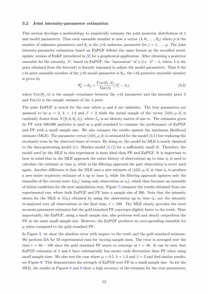
of initial conditions for the next assimilation step. Figure 7 compares the results obtained from one
experimental run, where both EnPGF and PF have a sample size of 200. Note that the intensity
shown for the MLE is λ(tk) obtained by using the observation up to time tk, not the intensity
re-analysed over all observations at the final time, t = 100. The MLE clearly provides the most
accurate parameter estimates but the gold-standard PF converges slightly faster to the truth. More
importantly, the EnPGF, using a small sample size, also performs well and clearly outperform the
PF at the same small sample size. However, the EnPGF produces an over-spreading ensemble for
µ when compared to the gold standard PF.
In Figure 8, we show the absolute error with respect to the truth and the gold standard estimate.
We perform DA for 50 experimental runs for varying sample sizes. The error is averaged over the
time t = 40 − 100 since the gold standard PF starts to converge at t = 40. It can be seen that
EnPGF estimates of λ and k have substantially less monte carlo fluctuation than PF when using
small sample sizes. We also test the case where µ = 0.5, k = 1.2 and β = 2 and find similar results,
see Figure 9. This demonstrates the strength of EnPGF over PF in a small sample size. As for the
MLE, the results in Figures 8 and 9 show a high accuracy of the estimate for the true parameters;
12
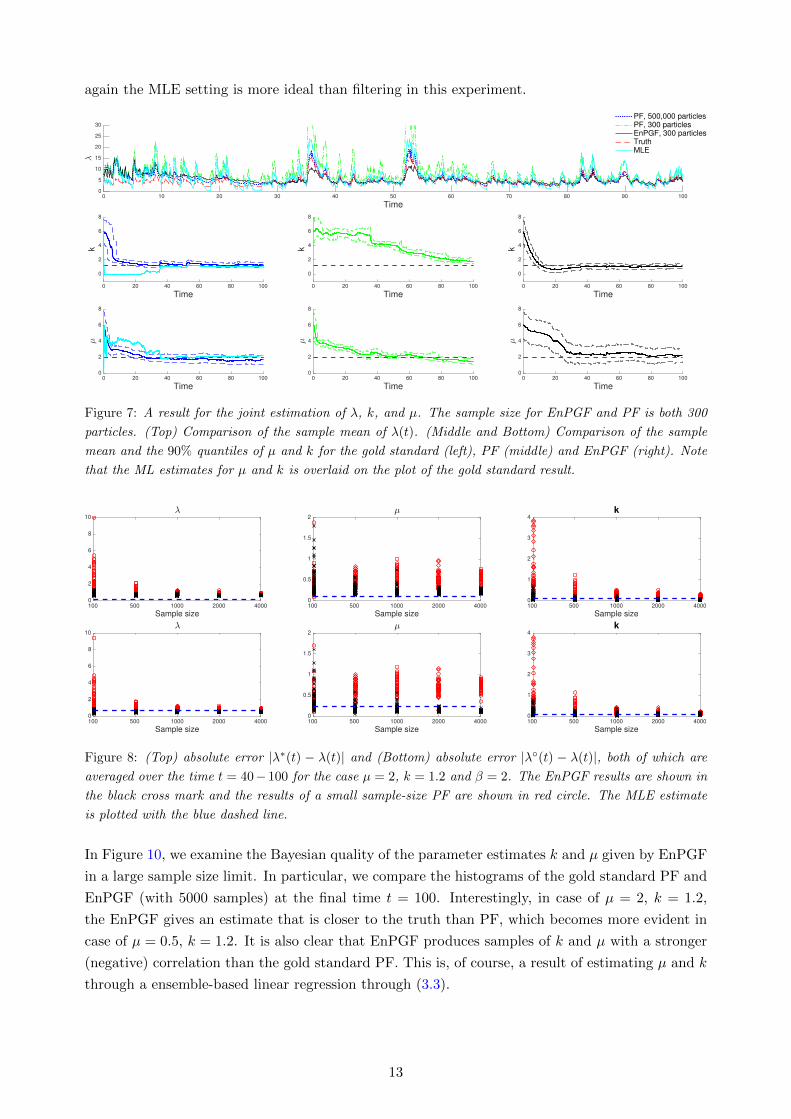
again the MLE setting is more ideal than filtering in this experiment.
0 10 20 30 40 50 60 70 80 90 100
Time
0
5
10
15
20
25
30
λ
PF, 500,000 particlesPF, 300 particlesEnPGF, 300 particlesTruthMLE
0 20 40 60 80 100
Time
0
2
4
6
8
k
0 20 40 60 80 100
Time
0
2
4
6
8
µ
0 20 40 60 80 100
Time
0
2
4
6
8
k
0 20 40 60 80 100
Time
0
2
4
6
8
µ
0 20 40 60 80 100
Time
0
2
4
6
8
k
0 20 40 60 80 100
Time
0
2
4
6
8
µ
Figure 7: A result for the joint estimation of λ, k, and µ. The sample size for EnPGF and PF is both 300
particles. (Top) Comparison of the sample mean of λ(t). (Middle and Bottom) Comparison of the sample
mean and the 90% quantiles of µ and k for the gold standard (left), PF (middle) and EnPGF (right). Note
that the ML estimates for µ and k is overlaid on the plot of the gold standard result.
100 500 1000 2000 4000
Sample size
0
2
4
6
8
10λ
100 500 1000 2000 4000
Sample size
0
0.5
1
1.5
2µ
100 500 1000 2000 4000
Sample size
0
1
2
3
4k
100 500 1000 2000 4000
Sample size
0
2
4
6
8
10λ
100 500 1000 2000 4000
Sample size
0
1
2
3
4k
100 500 1000 2000 4000
Sample size
0
0.5
1
1.5
2µ
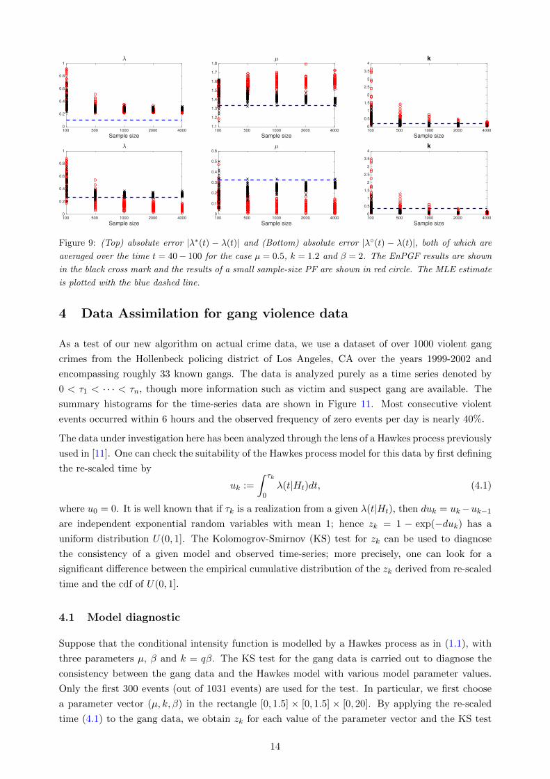
Figure 8: (Top) absolute error |λ∗(t) − λ(t)| and (Bottom) absolute error |λ◦(t) − λ(t)|, both of which are
averaged over the time t = 40− 100 for the case µ = 2, k = 1.2 and β = 2. The EnPGF results are shown in
the black cross mark and the results of a small sample-size PF are shown in red circle. The MLE estimate
is plotted with the blue dashed line.
In Figure 10, we examine the Bayesian quality of the parameter estimates k and µ given by EnPGF
in a large sample size limit. In particular, we compare the histograms of the gold standard PF and
EnPGF (with 5000 samples) at the final time t = 100. Interestingly, in case of µ = 2, k = 1.2,
the EnPGF gives an estimate that is closer to the truth than PF, which becomes more evident in
case of µ = 0.5, k = 1.2. It is also clear that EnPGF produces samples of k and µ with a stronger
(negative) correlation than the gold standard PF. This is, of course, a result of estimating µ and k
through a ensemble-based linear regression through (3.3).
13
100 500 1000 2000 4000
Sample size
0
0.2
0.4
0.6
0.8
1λ
100 500 1000 2000 4000
Sample size
1.1
1.2
1.3
1.4
1.5
1.6
1.7
1.8µ
100 500 1000 2000 4000
Sample size
0
0.5
1
1.5
2
2.5
3
3.5
4k
100 500 1000 2000 4000
Sample size
0
0.2
0.4
0.6
0.8
1λ
100 500 1000 2000 4000
Sample size
0
0.1
0.2
0.3
0.4
0.5
0.6µ
100 500 1000 2000 4000
Sample size
0
0.5
1
1.5
2
2.5
3
3.5
4k
Figure 9: (Top) absolute error |λ∗(t) − λ(t)| and (Bottom) absolute error |λ◦(t) − λ(t)|, both of which are
averaged over the time t = 40− 100 for the case µ = 0.5, k = 1.2 and β = 2. The EnPGF results are shown
in the black cross mark and the results of a small sample-size PF are shown in red circle. The MLE estimate
is plotted with the blue dashed line.
4 Data Assimilation for gang violence data
As a test of our new algorithm on actual crime data, we use a dataset of over 1000 violent gang
crimes from the Hollenbeck policing district of Los Angeles, CA over the years 1999-2002 and
encompassing roughly 33 known gangs. The data is analyzed purely as a time series denoted by
0 < τ1 < · · · < τn, though more information such as victim and suspect gang are available. The
summary histograms for the time-series data are shown in Figure 11. Most consecutive violent
events occurred within 6 hours and the observed frequency of zero events per day is nearly 40%.
The data under investigation here has been analyzed through the lens of a Hawkes process previously
used in [11]. One can check the suitability of the Hawkes process model for this data by first defining
the re-scaled time by
uk :=
∫ τk
0λ(t|Ht)dt, (4.1)
where u0 = 0. It is well known that if τk is a realization from a given λ(t|Ht), then duk = uk−uk−1are independent exponential random variables with mean 1; hence zk = 1 − exp(−duk) has a
uniform distribution U(0, 1]. The Kolomogrov-Smirnov (KS) test for zk can be used to diagnose
the consistency of a given model and observed time-series; more precisely, one can look for a
significant difference between the empirical cumulative distribution of the zk derived from re-scaled
time and the cdf of U(0, 1].
4.1 Model diagnostic
Suppose that the conditional intensity function is modelled by a Hawkes process as in (1.1), with
three parameters µ, β and k = qβ. The KS test for the gang data is carried out to diagnose the
consistency between the gang data and the Hawkes model with various model parameter values.
Only the first 300 events (out of 1031 events) are used for the test. In particular, we first choose
a parameter vector (µ, k, β) in the rectangle [0, 1.5] × [0, 1.5] × [0, 20]. By applying the re-scaled
time (4.1) to the gang data, we obtain zk for each value of the parameter vector and the KS test
14

0.2 0.4 0.6 0.8 1 1.2 1.4 1.6 1.8
k
0.5
1
1.5
2
2.5
3
3.5
4
µ
0.2 0.4 0.6 0.8 1 1.2 1.4 1.6 1.8
k
0.5
1
1.5
2
2.5
3
3.5
4
µ
0.5 1 1.5 2 2.5
k
0.2
0.4
0.6
0.8
1
1.2
1.4
µ
0.5 1 1.5 2 2.5
k
0.2
0.4
0.6
0.8
1
1.2
1.4
µ
Figure 10: Joint histograms at the final time t = 100 of the gold stadard PF (Left) and EnPGF with 5000
sample (Right) for the case µ = 2, k = 1.2 (Top) and µ = 0.5, k = 1.2 (Bottom). The cross mark is the true
parameter values.
is used to compare zk and the uniform distribution as described above. The results are shown in
Figure 12 and it can be seen that that parameter values for which the P-value of the KS test is
above 0.1 is clearly within the 95% confidence interval, which is well approximated by the formula
1.36/√n+
√n/10 for the length of observation n > 40 [7]. The geometry of these parameters
suggests a broad range of potential values for the decay rate β. The projection of the parameters
with P-value above 0.1 onto the (µ, k) plane for various values of β is plotted in Figure 13. It is
quite intuitive that the correlation between µ and k is negative for all fixed values of β since having
a larger µ would require a smaller k in order to explain the same data. Similarly, a large value of
µ would be required for a larger value of β in order to achieve consistency with the data.
We also estimate the parameters using the maximum likelihood estimator (MLE) for the first 300
events in the data. The likelihood function of the Hawkes process can be found in [21]. The
optimization of likelihood is computed based on a Nelder-Mead simplex algorithm in MATLAB.
As shown in Figure 12, the MLE lies within the set of parameters with P-value from the KS test
above 0.1. We will later use the parameters with a large P-value as the initial knowledge of the
model parameters in the Bayesian framework.
15

Figure 11: (Left) Histogram of time between two events in a unit of one day. (Right) Histogram of the
number of violence crime event per day
Figure 12: (Left) KS plot of zk for the Hawkes model. The dash lines indicate the 95% confidence bound
and the green curves are the (observed) cumulative distribution obtained from simulated time-series with
parameter values with P-values over 0.1. The black curve is the cumulative distribution of a time-series
simulated with the MLE. (Middle) A histogram of P-values for uniform parameter grid points (k, β, µ) in
[0, 1.5]× [0, 20]× [0, 1.5]. (Right) The blue dots shows those parameter with P-value between 0.1 and 0.2 and
the red dots shows those with P-value over 0.2. The MLE is shown in the dark + marker.
4.2 Sequential Data Assimilation
We now apply EnPGF and PF to jointly track the intensity process λ(t) and model parameters
for the Hollenbeck gang violence data. Again, we use (3.1) as a forecast model for λ(t), where we
choose δt = 1/6 days, i.e., every 4 hours. As discussed earlier, the range of likely values of β is
very broad, so we fix its value to β = 2 and try to track only the parameters µ and k. We use two
different initializations:
Initialization 1: The data during the first 300 days is used to initialize the ensemble of parameters
through the KS test as already done in Section 4.1. In particular, we use the parameters on the
plane β = 2 with the P-value greater than 0.1, see again Figure 12, as the initial set of parameters.
If a sample size M is desired, M particles are randomly drawn from the finite set of the initial
parameters and then perturbed with a normal noise N(0, 0.01I2). We then choose the initial sample
λi(0) to be the same as µi for i = 1, . . . ,M .
Initialization 2: We draw initial sample (λi(0), µi, ki) from a multivariate normal distribution
N([6, 3, 3], 0.1I3).
16

Figure 13: Projection of the parameters with P-valaue above 0.1 onto the (µ, k) plane for various values of
β, see also Figure 12
We estimate the filtered distribution of (λ(t), µ, k) in the time interval [300, 600] using PF with
200,000 samples for the above two initializations. We test EnPGF with 100 samples using the ini-
tialization 2. The results in Figure 14 shows that the estimation given by PF with initialization-1
parameters are relatively stable over the whole data assimilation period. In addition, the sample
computed from PF with the initialization 2 converges to the sample of the initialization-1 parame-
ters. This suggests that the set of parameters found by KS indeed agrees well with the parameters
tracked by the PF algorithm. The sample generated by EnPGF, see also Figure 14, show a similar
convergence but with a noticeable discrepancy in the parameter k. The empirical distribution at
the final time is compared in Figure 15. The marginal distribution of λ and joint distribution of
µ and k after the final data assimilation time step are compared for the cases of PF and EnPGF,
both with initialization 2. The sample supports of the two results mostly overlap but the sample
of EnPGF seems to be relatively overspreading.
5 Predictability and forecast skills
5.1 Predictability
The “predictability” of an event can be defined in many ways. We focus on a forecast system that
releases an “indicator” to alarm an upcoming event of interest. For example, in the context of
police patrolling, once patrol officers complete their current assignment, a forecast system may try
to suggest the location where criminal activity is most likely to happen within the next hour. In
the current time-series application, this kind of forecast system is simplified to predicting whether
or not the next violence crime would occur within the next H unit of times. After the intensity
is updated as a result of the n-th observed violence at time τn, we wish to use the intensity of
the Hawkes process at τn as an indicator variable. Therefore, we may choose a threshold of the
intensity, denoted by `, so that whenever λ(τn) > `, the forecast system will suggest to the user
that τn+1 − τn < H. As such, the event we wish to predict can be considered as a binary event,
say, Y = 1 if τn+1 − τn < H and Y = 0 otherwise. The so-called “hit rate” is defined by
H(`) := Pr(λ(τn) > `|Y = 1),
and the “false alarm rate” by
F(`) := Pr(λ(τn) > `|Y = 0).
17

0 50 100 150 200 250 300
Time
0
2
4
6
8
10λ
PF: Initialization 1
PF: Initialization 2
EnPGF: Initialization 2
0 50 100 150 200 250 300
Time
0
1
2
3
4
k
0 50 100 150 200 250 300
Time
0
1
2
3
4
µ
0 50 100 150 200 250 300
Time
0
1
2
3
4
k
0 50 100 150 200 250 300
Time
0
1
2
3
4
µ
Figure 14: The results for the joint estimation of λ, k, and µ for Holenbeck gang violence data in the interval
[300, 600].
The relative characteristic curve (ROC), which is a graph of the pair (F(`),H(`)) for various
values of `, can be used to measure the performance of a forecast system. We are interested in
measuring the performance of two intensity-based forecast systems: (1) the ensemble mean of PF
and (2) Hawkes process with parameters obtained from MLE. As suggested in [5], the hit rate and
false alarm rate can be empirically estimated by the observed frequencies. Suppose that we have
the indicator-observation pairs (λJ , y(J)) for J = 1, . . . , n, sorted in ascending order such that
λ1 ≤ λ2 ≤ · · · ≤ λn and y(J) is the observation corresponding to λJ . The empirical hit rate and
false alarm rate are given by
H(J) = 1− 1
N1
J∑m=1
y(J), F(J) = 1− 1
N0
J∑m=1
1− y(J),
where N1 is the number of events y(J) = 1 and N0 = n − N1. The ROC plot is the graph
(F(J),H(J)) and its area under the curve (AUC) is usually used to diagnose the association
between the indicator variable and the observation. The AUC close to 1 is desired while AUC of
1/2 would suggest zero association. For empirical ROC, the AUC can be approximated by
AUC =1
N0N1
( n∑J=1
ny(J)− N1(1 +N1)
2
).
To understand the accuracy of the above forecast system in different parameter regimes of the
Hawkes process, we simulated 100 sample paths for various parameters and approximate AUC in
each case, assuming that all true parameters are known. The pairs (λJ , y(J)) in this case is the
intensity at the time of observation and y(J) = 1 if the the subsquent gang-related violence occurs
18

0 1 2 3 4 5 6
λ
0
0.05
0.1
0.15
0.2
0.25
0.3
0.35
λPF: initialization 2
EnPGF:initialization 2
0
0.2
0.4
0.6
0.8
1
1.2
1.4
1.6
1.8
2
µ
0 0.5 1 1.5 2
k
Figure 15: (Left) Comparing the historgram of λ for PF (200,000 particles) with EnPGF (100 particles),
both of which use the initialization 2. (Right) Empirical joint distribution of k, and µ at the final step for
the gang violence data, which is initialized by using the sample spread obtained from the KS test with the
p-values above 0.1. The sample of 100-member EnPGF with the initialization 2 is shown in the solid black
dots on top of the approximated density obtained from PF
within a certain H unit of time; we set H = 0.1 in the experiment. All parameters we used yield
the same expected intensity, E[λ] = 4. Figure 16 shows that if the data is generated truly from a
Hawke process and we can precisely identify the parameters, the ability of the above intensity-driven
forecast system would depend on the parameter regime the data comes from, “low predictability”
or ”highly predictable” regimes. The former usually has a relatively large µ and small k/β while
the latter has a relatively small µ and k/β being close to 1. This is intuitive because in the highly
predictable regime the event is unlikely to be generated by the baseline intensity µ and most events
are actually the “offspring” of the preceding events. Recall that the ratio k/β describes the fraction
of events that are endogenously generated by the previous event. Thus, whenever the intensity is
above the baseline, the clustering is imminent. This allows the intensity-driven forecast system to
achieve a reliable forecast. Thus, for µ = 2, k = 1 and β = 2, the AUC results is poor (i.e. being
slightly above 1/2), see Figure 16. On the other hand, the parameter regime where µ � 1 and
k/β → 1 is clearly more predictable in a sense that we would be able to find a threshold ` that
produces a high hit rate with a low false alarm rate as seen from the “knee point” bending toward
upper left corner of the ROC plot. Also, it can be seen from Figure 16 that increasing both k and
β simultaneously while keeping their ratio constant can also increase the predictability.
5.2 Evaluation of forecast skills
It is usually true that most crime models are imperfect (i.e. the crime data are not exactly generated
by the models). Identifying model errors based on the data is a challenging task. Thus, in most
occasions, we may insist to use the model, knowing that it may have model error. In this section,
we will first allow the presence of artificial model error in the synthetic experiment and evaluate
19
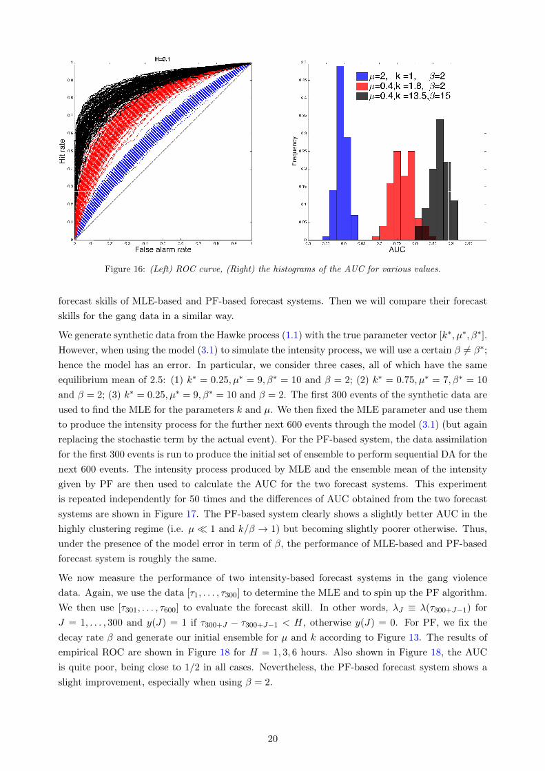
Figure 16: (Left) ROC curve, (Right) the histograms of the AUC for various values.
forecast skills of MLE-based and PF-based forecast systems. Then we will compare their forecast
skills for the gang data in a similar way.
We generate synthetic data from the Hawke process (1.1) with the true parameter vector [k∗, µ∗, β∗].
However, when using the model (3.1) to simulate the intensity process, we will use a certain β 6= β∗;
hence the model has an error. In particular, we consider three cases, all of which have the same
equilibrium mean of 2.5: (1) k∗ = 0.25, µ∗ = 9, β∗ = 10 and β = 2; (2) k∗ = 0.75, µ∗ = 7, β∗ = 10
and β = 2; (3) k∗ = 0.25, µ∗ = 9, β∗ = 10 and β = 2. The first 300 events of the synthetic data are
used to find the MLE for the parameters k and µ. We then fixed the MLE parameter and use them
to produce the intensity process for the further next 600 events through the model (3.1) (but again
replacing the stochastic term by the actual event). For the PF-based system, the data assimilation
for the first 300 events is run to produce the initial set of ensemble to perform sequential DA for the
next 600 events. The intensity process produced by MLE and the ensemble mean of the intensity
given by PF are then used to calculate the AUC for the two forecast systems. This experiment
is repeated independently for 50 times and the differences of AUC obtained from the two forecast
systems are shown in Figure 17. The PF-based system clearly shows a slightly better AUC in the
highly clustering regime (i.e. µ� 1 and k/β → 1) but becoming slightly poorer otherwise. Thus,
under the presence of the model error in term of β, the performance of MLE-based and PF-based
forecast system is roughly the same.
We now measure the performance of two intensity-based forecast systems in the gang violence
data. Again, we use the data [τ1, . . . , τ300] to determine the MLE and to spin up the PF algorithm.
We then use [τ301, . . . , τ600] to evaluate the forecast skill. In other words, λJ ≡ λ(τ300+J−1) for
J = 1, . . . , 300 and y(J) = 1 if τ300+J − τ300+J−1 < H, otherwise y(J) = 0. For PF, we fix the
decay rate β and generate our initial ensemble for µ and k according to Figure 13. The results of
empirical ROC are shown in Figure 18 for H = 1, 3, 6 hours. Also shown in Figure 18, the AUC
is quite poor, being close to 1/2 in all cases. Nevertheless, the PF-based forecast system shows a
slight improvement, especially when using β = 2.
20

0 5 10 15 20 25 30 35 40 45 50-0.03
-0.02
-0.01
0
0.01
0.02
0.03
0.04
AU
C(M
LE
)-A
UC
(PF
)
µ=1.5, k=4, β=10
µ=0.75, k=7,β=10
µ=0.25, k=9, β=10
Figure 17: Differences in the emperical AUC obtained from PF-based and MLE-based forecast systems tested
for 50 independent experiments. The negative value means the PF-based system results in a higher AUC and
vice versa.
0 0.2 0.4 0.6 0.8 1
False alarm rate
0
0.1
0.2
0.3
0.4
0.5
0.6
0.7
0.8
0.9
1
Hit r
ate
H=6, 73 events
PF: β=2, AUC=0.5813PF: β=4, AUC=0.5689
PF: β=8 AUC=0.5623MLE: AUC=0.5224
0 0.2 0.4 0.6 0.8 1
False alarm rate
0
0.1
0.2
0.3
0.4
0.5
0.6
0.7
0.8
0.9
1
Hit r
ate
H=3, 42 events
PF: β=2, AUC=0.5536
PF: β=4, AUC=0.5456PF: β=8 AUC=0.5037MLE: AUC=0.5133
0 0.2 0.4 0.6 0.8 1
False alarm rate
0
0.1
0.2
0.3
0.4
0.5
0.6
0.7
0.8
0.9
1
Hit r
ate
H=1, 14 events
PF: β=2, AUC=0.5787PF: β=4, AUC=0.5065
PF: β=8 AUC=0.3915MLE: AUC=0.5469
Figure 18: Emperical ROC of PF-based forecast systems for different values of β and the Hawkes process
with the MLE parameters.
6 Conclusion
In this paper we have introduced a novel sequential data assimilation ensemble Poisson-Gamma
filtering (EnPGF) algorithm for discrete-time filtering suitable for real-time crime data. The ad-
vantage of sequentially updating the forecast in real-time while taking into account uncertainty in
model parameters could have a significant impact on predictive policing software which currently
uses MLE. The ensemble mean of EnPGF is used not only to track the true signal, which is the
crime intensity rate in this case, but also approximate the parameter of the Hawkes process. In
the numerical experiments, the tracking skill is justified by comparing the estimate with the true
signal and the particle filtering (PF) in the large sample size limit. The key strength of EnPGF
over PF is its improved accuracy as well as less monte-carlo fluctuation in the case of small sample
size. For the real-world time-series of gang violence data, the validity of EnPGF is testified by com-
paring with PF and the “likely” parameter region identified by the Kolmogrov-Smirnov statistics.
We showed that the results from these distinct data analysis methods happen to agree very well.
Nevertheless, our experimental results suggest an issue where EnPGF tends to produce over/under-
21

spreading ensemble for some parameter estimates; hence probabilistically over/under-confidence in
the parameter estimates. The implication of this in term of forecasting would also be an interesting
future work. Although we demonstrate the application of the new method only to time-series data,
the extension to high-dimensional spatio-temporal data can be achieved by serially processing M
grid cell time-series analysis one at a time and use the ensemble updated through data assimilation
of the first grid cell as a new prior for data assimilation in the second grid cell and so on. This
serially-updated formulation is one of the commonly used implementations for EnKF [2]. Our work
underway will develop this high-dimensional extension of EnPGF and study its effectiveness with
burglary data.
In this paper we have also examined the forecast skills provided by sequential data assimilation
for the time-series Hawkes model which is crucial for determining the usefulness of any predictive
policing software. We carried out sequential data assimilation using a particle filter with a large
sample size to construct the ensemble forecast. We then studied the forecast system whereby
the elevated risk is alerted whenever the crime intensity rate predicated by the ensemble forecast
exceeds a given threshold. Thus, the ROC analysis is a suitable tool to study the ability of such a
forecast system. For the gang violence data, our results show that data assimilation gives a small
improvement in the forecast skill compared with the data-driven Hawkes process, in which the
stochastic part in (1.1) is substituted by the observed data. The latter is, in fact, analogous to the
ETAS system. A small improvement would be highly important to predictive policing software,
since one can never expect to have a perfect model of urban crime, so making improvements in the
assimilation step are where one can hope to make significant gains.
Acknowledgments. NS gratefully acknowledges the support of the UK Engineering and Physical
Sciences Research Council for programme grant EP/P030882/1. MBS gratefully acknowledges the
support of the US National Science Foundation grant DMS-1737925.
Appendix A: Derivation of (3.2)
We define the quantities M(t) := E[λ(t)] and V (t) := Var[λ(t)] to be the mean and variance of the
state space model defined in (3.1). We compute M(t+ h) as follows
M(t+ h) =E[λ(t+ h)],
=E[E[λ(t+ h)|λ(t)]],
=E[µβh+ (1 + (k − β)h)λ(t)]
=µβh+ (1 + (k − β)h)M(t).
Hence, we find subtracting M(t) from both sides, dividing by h and taking the limit h → 0, that
we get the first ODE in (3.2).
22

The second ODE in (3.2) is found by computing V (t+ h) as follows
V (t+ h) =Var[λ(t+ h)],
=E[Var[λ(t+ h)|λ(t)] + Var[E[λ(t+ h)|λ(t)]],
=E[k2Var[N(t)]] + Var[µβh+ (1 + (k − β)h)λ(t)],
=E[k2λh] + (1 + (k − β)h)2Var[λ(t)],
=hk2M(t) + (1 + (k − β)h)2V (t).
Subtracting V (t) from both sides, dividing by h and taking the limit h→ 0, that we get the second
ODE in (3.2).
The system (3.2) has the general solution
M(t) =µβ
β − k+
(µ+m0(k − β))
k − 1e(k−β)t,
V (t) =1
2(k − β)2
(µβk2 − 2(µ+m0(k − β))k2e(k−β)t + (µβk2 + 2v0(k − β)2 + 2k2(k − β)m0)e
2(k−β)t),
where M(0) = m0, V (0) = v0. In particular, the equilibrium state is given by
M =µβ
β − k, V =
µβk2
2(β − k)2.
Appendix B: Resampling
In the resampling step, particles with low weights are removed with high probabilities and particles
with high weights are multiplied. Thus the computation can be focused on those particles that
are relevant to the observations. There are a number of resampling algorithms and most common
algorithms are unbiased; hence the key difference in performance lies in the variance reduction,
see [9] for a review and comparison of common resampling schemes. The most basic algorithm is
the so-called simple random resampling introduced in Gordon, which is also known as multinomial
resampling. Suppose that the original set of weighted particles is {wj , vj} for j = 1, . . . ,M . The
simple resampling generate a new set of particles {1/M, v∗k} for k = 1, . . . ,M based on the inverse
cumulative density function (CDF):
Step 1 Simulate a uniform random number uk ∼ U [0, 1) for k = 1, . . . ,M
Step 2 Assign v∗k = vi if uk ∈ (qi−1, qi], where qi =∑i
s=1ws.
In this work, we use the residual resampling algorithm introduced in [18] to reduce the monte carlo
variance of the simple random resampling. In this approach, we replicate Nj exact copies of vj
accodring to
Nj = bMwjc+ Nj ,
where bc denotes the integer part and Ni for j = 1, . . . ,M are distributed according to the multi-
nomial distribution with the number of trials M −∑M
j=1bMwjc and probability of success
pj =Mwj −
∑Mj=1bMwjc
M −∑M
j=1bMwjc.
23

The simple resampling scheme can be used to select the remaining M −∑M
j=1bMwjc particles;
hence obtaining Nj .
The resampling scheme should be used only when it is necessary since by selecting out only high-
weight particles, it causes the particle depravation. A criterion to activate the resampling step in
particle filtering is usually done by setting a certain threshold for the effective sample size, defined
by
Neff =1∑M
i=1w2i
.
In this work, we use the resampling step only when Neff < 1/8.
References
[1] J. L. Anderson. An ensemble adjustment kalman filter for data assimilation. Mon. Wea. Rev.,
129:2884–2903, 2001.
[2] J. L. Anderson. A local least squares framework for ensemble filtering. Weather Rev., 131(doi:
10.1175/1520-0493):634–642, 2003.
[3] C. H. Bishop. The gigg-enkf: ensemble kalman filtering for highly skewed non-negative uncer-
stianty distribution. Q. J. R. Meteorol. Soc., 142:1395–1412, 2016.
[4] C. H. Bishop, B. J. Etherton, and S. J. Majumdar. Adaptive sampling with the ensemble
transform kalman filter. part i: Theoretical aspects. Mon. Wea. Rev., 129:420–436, 2001.
[5] J. Broecker. Forecast Verification: A Practitioner’s Guide in Atmospheric Science, chapter
Probability Forecasts, pages 119–139. John Wiley & Sons, Ltd., 2012.
[6] G. Burgers, P. J. van Leeuwen, and G. Evensen. Analysis scheme in the ensemble kalman
filter. Mon. Wea. Rev., 126:1719–1724, 1998.
[7] W. J. Conover. Practical nonparametric statistics. John Wiley & Sons, 1999.
[8] D. Crisan and A. Doucet. A survey of convergence results on particle filtering for practitioners.
IEEE Transaction on Signal Processing, 50(3):736–746, 2002.
[9] R. Douc. Comparison of resampling schemes for particle filtering. Image and Signal Processing
and Analysis. IEEE, 2005.
[10] A. Doucet, N. de Freitas, and N. Gordon. Sequential Monte-Carlo methods in practice.
Springer-Verlag, 2001.
[11] Mike Egesdal, Chris Fathauer, Kym Louie, Jeremy Neuman, George Mohler, and Erik Lewis.
Statistical and stochastic modeling of gang rivalries in los angeles. SIAM Undergraduate Re-
search Online, pages 72–94, 2010.
[12] G. Evensen. Sequential data assimilation with a nonlinear quasi-geostrophic model using monte
carlo methods to forecast error statistics. J. Geophys. Res., 99(C5):10143–10162, 1994.
[13] N. J. Gordon, D. J. Salmond, and A. F. M. Smith. Novel approach to nonlinear/non-gaussian
bayesian state estimation. Rad. and Sig. Pro., IEE Proc. F, 140(2):107–113, 1993.
24
[14] H. Guillaud. Police predictive : la prediction des banalites. http://internetactu.blog.
lemonde.fr/2015/06/27/police-predictive-la-prediction-des-banalites/, June
2015. Online; accessed 21-Sept-2017.
[15] P. L. Houtekamer and H. L. Mitchell. Data assimilation using an ensemble kalman filter
technique. Mon. Wea. Rev., 126:796–811, 1998.
[16] K. Law, A. Stuart, and K. Zygalakis. Data Assimilation: Mathematical Introduction. Springer-
Verlag, 2015.
[17] P. Jan Van Leeuwen, Y. Cheng, and S. Reich. Nonlinear Data Assimilation. Frontier in
Applied Dynamical Systems: Reviewer and Tutorial. Springer, 2015.
[18] J. Liu and R. Chen. Sequential monte carlo methods for dynamic systems. J. Roy. Statist.
Soc. Ser. B, 93:1032–1044, 1998.
[19] G. O. Mohler et al. Self-exciting point process modeling of crime. J. of the American Stat.
Assoc., 106(493):100–108, 2011.
[20] George O Mohler, Martin B Short, Sean Malinowski, Mark Johnson, George E Tita, Andrea L
Bertozzi, and P Jeffrey Brantingham. Randomized controlled field trials of predictive policing.
Journal of the American statistical association, 110(512):1399–1411, 2015.
[21] Y. Ogata. On lewis’ simulation method for point process. IEEE Transactions on Information
Theory, IT-27(1):23–31, 1981.
25
Top Related