


Languages
Pages
Legal


Regression Analysis: Case Study 2
Dr. Kempthorne
September 30, 2013
Contents
1 Linear Regression Models for Exchange Rate Regimes 21.1 Exchange Rate Data . . . . . . . . . . . . . . . . . . . . . . . . . 21.2 Exchange Rate Regimes for the Chinese Yuan . . . . . . . . . . . 41.3 Converting from USD Base to Swiss Franc Base . . . . . . . . . . 51.4 Linear Regression Models of Currency Returns . . . . . . . . . . 7
1
1 Linear Regression Models for Exchange RateRegimes
1.1 Exchange Rate Data
The Federal Reserve Economic Database (FRED) provides historical daily ex-change rates of all major currencies in the world.
An R script (“fm casestudy fx 1.r”) collects these data and stores them inthe R workspace “fm casestudy fx 1.RData”.
The following commands re-load the data and provide details explaining thedata.
> # 0.1 Install/load libraries
> source(file="fm_casestudy_0_InstallOrLoadLibraries.r")
> # 0.2 Load R workspace created by script fm_casestudy_fx_1.r
> load(file="fm_casestudy_fx_1.Rdata")
> # 1.0 Extract time series matrix of exchange rates for symbols given by list.symbol0 ----
>
> list.symbol0<-c("DEXCHUS", "DEXJPUS", "DEXKOUS", "DEXMAUS",
+ "DEXUSEU", "DEXUSUK", "DEXTHUS", "DEXSZUS")
> fxrates000<-fred.fxrates.00[,list.symbol0]
> dim(fxrates000)
[1] 3704 8
> head(fxrates000)
DEXCHUS DEXJPUS DEXKOUS DEXMAUS DEXUSEU DEXUSUK DEXTHUS DEXSZUS
1999-01-04 8.2793 112.15 1187.5 3.8 1.1812 1.6581 36.20 1.3666
1999-01-05 8.2795 111.15 1166.0 3.8 1.1760 1.6566 36.18 1.3694
1999-01-06 8.2795 112.78 1160.0 3.8 1.1636 1.6547 36.50 1.3852
1999-01-07 8.2798 111.69 1151.0 3.8 1.1672 1.6495 36.30 1.3863
1999-01-08 8.2796 111.52 1174.0 3.8 1.1554 1.6405 36.45 1.3970
1999-01-11 8.2797 108.83 1175.0 3.8 1.1534 1.6375 36.28 1.3963
> tail(fxrates000)
DEXCHUS DEXJPUS DEXKOUS DEXMAUS DEXUSEU DEXUSUK DEXTHUS DEXSZUS
2013-09-13 6.1186 99.38 1085.88 3.2880 1.3276 1.5861 31.81 0.9319
2013-09-16 6.1198 98.98 1081.34 3.2880 1.3350 1.5927 31.66 0.9258
2013-09-17 6.1213 99.16 1082.15 3.2455 1.3357 1.5901 31.68 0.9266
2013-09-18 6.1210 99.04 1081.40 3.2320 1.3351 1.5965 31.65 0.9260
2013-09-19 6.1210 99.33 1070.88 3.1455 1.3527 1.6043 31.03 0.9112
2013-09-20 6.1210 99.38 1076.02 3.1640 1.3522 1.6021 31.04 0.9104
>
> # Print symbol/description/units of these rates from data frame fred.fxrates.doc
2

> options(width=120)
> print(fred.fxrates.doc[match(list.symbol0, fred.fxrates.doc$symbol),
+ c("symbol0", "fx.desc", "fx.units")])
symbol0 fx.desc fx.units
3 DEXCHUS China / U.S. Foreign Exchange Rate Chinese Yuan to 1 U.S. $
7 DEXJPUS Japan / U.S. Foreign Exchange Rate Japanese Yen to 1 U.S. $
8 DEXKOUS South Korea / U.S. Foreign Exchange Rate South Korean Won to 1 U.S. $
9 DEXMAUS Malaysia / U.S. Foreign Exchange Rate Malaysian Ringgit to 1 U.S. $
20 DEXUSEU U.S. / Euro Foreign Exchange Rate U.S. $ to 1 Euro
22 DEXUSUK U.S. / U.K. Foreign Exchange Rate U.S. $ to 1 British Pound
18 DEXTHUS Thailand / U.S. Foreign Exchange Rate Thai Baht to 1 U.S. $
16 DEXSZUS Switzerland / U.S. Foreign Exchange Rate Swiss Francs to 1 U.S. $
> # Plot exchange rate time series in 2x2 panels
> par(mfcol=c(2,2))
> for (j0 in c(1:ncol(fxrates000))){
+ plot(fxrates000[,j0],
+ main=dimnames(fxrates000)[[2]][j0])
+ }
Jan 04 1999 Jul 03 2006 Jun 28 2013
6.5
7.0
7.5
8.0
DEXCHUS
Jan 04 1999 Jul 03 2006 Jun 28 2013
8010
012
0
DEXJPUS
Jan 04 1999 Jul 03 2006 Jun 28 2013
900
1100
1400
DEXKOUS
Jan 04 1999 Jul 03 2006 Jun 28 2013
3.0
3.2
3.4
3.6
3.8
DEXMAUS
3
Jan 04 1999 Jul 03 2006 Jun 28 2013
0.8
1.0
1.2
1.4
1.6
DEXUSEU
Jan 04 1999 Jul 03 2006 Jun 28 2013
1.4
1.6
1.8
2.0
DEXUSUK
Jan 04 1999 Jul 03 2006 Jun 28 2013
3035
4045
DEXTHUS
Jan 04 1999 Jul 03 2006 Jun 28 2013
0.8
1.2
1.6
DEXSZUS
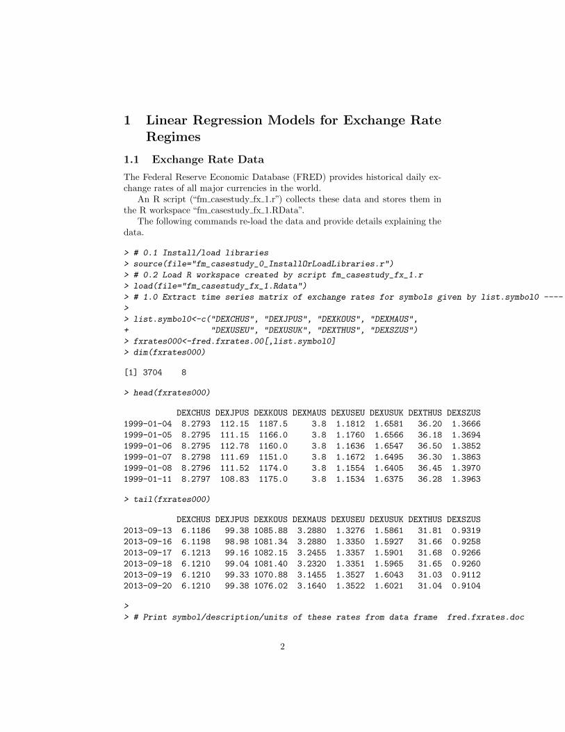
The time series matrix fxrates000 has data directly from the FRED website.
1.2 Exchange Rate Regimes for the Chinese Yuan
The Chinese Yuan was pegged to the US Dollar prior to July 2005. Then, Chinaannounced that the exchange rate would be set with reference to a basket ofother currencies, allowing for a movement of up to 0.3% movement within anygiven day. The actual currencies and their basket weights are unannounced byChina.
From an empirical standpoint, there are several important questions
• For any given period, what is the implicit reference basket for the Chinesecurrency?
• Has the reference basket changed over time?
• Has the Chinese currency depreciated with respect to the dollar?
If so, how much and when?
Frankel and Wei (1994) detail methodology for evaluating the implicit ex-change rate regime of a currency. The approach regesses changes in the targetcurrency on changes in the values of possible currencies in the reference basket.
To apply this methodology we re-express the dollar-based exchange ratesusing another currency, the Swiss Franc. This allows currency moves of the
4
dollar to be be used to explain moves in the Yuan. The choice of Swiss Franc isconsistent with evaluations with respect to a stable, developed-market currency.
1.3 Converting from USD Base to Swiss Franc Base
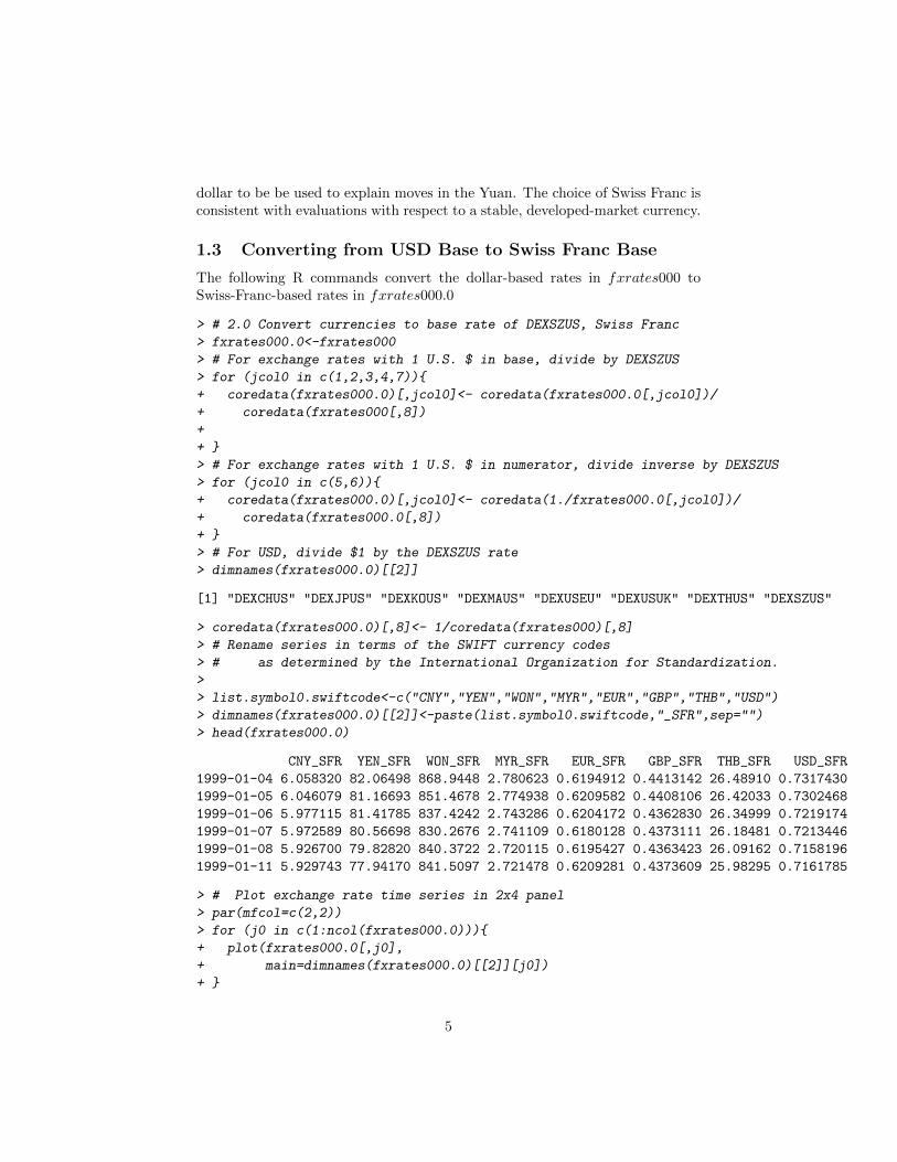
The following R commands convert the dollar-based rates in fxrates000 toSwiss-Franc-based rates in fxrates000.0
> # 2.0 Convert currencies to base rate of DEXSZUS, Swiss Franc
> fxrates000.0<-fxrates000
> # For exchange rates with 1 U.S. $ in base, divide by DEXSZUS
> for (jcol0 in c(1,2,3,4,7)){
+ coredata(fxrates000.0)[,jcol0]<- coredata(fxrates000.0[,jcol0])/
+ coredata(fxrates000[,8])
+
+ }
> # For exchange rates with 1 U.S. $ in numerator, divide inverse by DEXSZUS
> for (jcol0 in c(5,6)){
+ coredata(fxrates000.0)[,jcol0]<- coredata(1./fxrates000.0[,jcol0])/
+ coredata(fxrates000.0[,8])
+ }
> # For USD, divide $1 by the DEXSZUS rate
> dimnames(fxrates000.0)[[2]]
[1] "DEXCHUS" "DEXJPUS" "DEXKOUS" "DEXMAUS" "DEXUSEU" "DEXUSUK" "DEXTHUS" "DEXSZUS"
> coredata(fxrates000.0)[,8]<- 1/coredata(fxrates000)[,8]
> # Rename series in terms of the SWIFT currency codes
> # as determined by the International Organization for Standardization.
>
> list.symbol0.swiftcode<-c("CNY","YEN","WON","MYR","EUR","GBP","THB","USD")
> dimnames(fxrates000.0)[[2]]<-paste(list.symbol0.swiftcode,"_SFR",sep="")
> head(fxrates000.0)
CNY_SFR YEN_SFR WON_SFR MYR_SFR EUR_SFR GBP_SFR THB_SFR USD_SFR
1999-01-04 6.058320 82.06498 868.9448 2.780623 0.6194912 0.4413142 26.48910 0.7317430
1999-01-05 6.046079 81.16693 851.4678 2.774938 0.6209582 0.4408106 26.42033 0.7302468
1999-01-06 5.977115 81.41785 837.4242 2.743286 0.6204172 0.4362830 26.34999 0.7219174
1999-01-07 5.972589 80.56698 830.2676 2.741109 0.6180128 0.4373111 26.18481 0.7213446
1999-01-08 5.926700 79.82820 840.3722 2.720115 0.6195427 0.4363423 26.09162 0.7158196
1999-01-11 5.929743 77.94170 841.5097 2.721478 0.6209281 0.4373609 25.98295 0.7161785
> # Plot exchange rate time series in 2x4 panel
> par(mfcol=c(2,2))
> for (j0 in c(1:ncol(fxrates000.0))){
+ plot(fxrates000.0[,j0],
+ main=dimnames(fxrates000.0)[[2]][j0])
+ }
5

Jan 04 1999 Jul 03 2006 Jun 28 2013
56
78
CNY_SFR
Jan 04 1999 Jul 03 2006 Jun 28 2013
6070
8090
110
YEN_SFR
Jan 04 1999 Jul 03 2006 Jun 28 2013
600
1000
1400
WON_SFR
Jan 04 1999 Jul 03 2006 Jun 28 2013
2.5
3.0
3.5
4.0
MYR_SFR
6

Jan 04 1999 Jul 03 2006 Jun 28 2013
0.6
0.7
0.8
0.9
EUR_SFR
Jan 04 1999 Jul 03 2006 Jun 28 2013
0.4
0.6
0.8
GBP_SFR
Jan 04 1999 Jul 03 2006 Jun 28 2013
2530
3540
THB_SFR
Jan 04 1999 Jul 03 2006 Jun 28 2013
0.6
0.8
1.0
1.2
1.4
USD_SFR
1.4 Linear Regression Models of Currency Returns
> # 3.0 Compute daily price changes on the log scale
> # Due to missing data, fill in missing values with previous non-NA
> # To check for presence of missing values, execute
> # apply(is.na(fxrates000.0),2,sum)
> # If necessary apply
> # fxrates000.0<-na.locf(fxrates000.0)
> fxrates000.0.logret<-diff(log(fxrates000.0))
> dimnames(fxrates000.0.logret)[[2]]
[1] "CNY_SFR" "YEN_SFR" "WON_SFR" "MYR_SFR" "EUR_SFR" "GBP_SFR" "THB_SFR" "USD_SFR"
> par(mfcol=c(2,2))
> for (j0 in c(1:ncol(fxrates000.0.logret))){
+ plot(fxrates000.0.logret[,j0],
+ main=dimnames(fxrates000.0.logret)[[2]][j0])
+ }
7
Jan 04 1999 Jul 03 2006 Jun 28 2013
−0.
08−
0.02
0.04
CNY_SFR
Jan 04 1999 Jul 03 2006 Jun 28 2013
−0.
08−
0.02
0.02
YEN_SFR
Jan 04 1999 Jul 03 2006 Jun 28 2013
−0.
100.
000.
10
WON_SFR
Jan 04 1999 Jul 03 2006 Jun 28 2013
−0.
08−
0.02
0.02
MYR_SFR
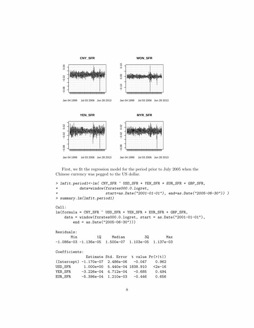
First, we fit the regression model for the period prior to July 2005 when theChinese currency was pegged to the US dollar.
> lmfit.period1<-lm( CNY_SFR ~ USD_SFR + YEN_SFR + EUR_SFR + GBP_SFR,
+ data=window(fxrates000.0.logret,
+ start=as.Date("2001-01-01"), end=as.Date("2005-06-30")) )
> summary.lm(lmfit.period1)
Call:
lm(formula = CNY_SFR ~ USD_SFR + YEN_SFR + EUR_SFR + GBP_SFR,
data = window(fxrates000.0.logret, start = as.Date("2001-01-01"),
end = as.Date("2005-06-30")))
Residuals:
Min 1Q Median 3Q Max
-1.086e-03 -1.136e-05 1.500e-07 1.103e-05 1.137e-03
Coefficients:
Estimate Std. Error t value Pr(>|t|)
(Intercept) -1.170e-07 2.486e-06 -0.047 0.962
USD_SFR 1.000e+00 5.440e-04 1838.910 <2e-16
YEN_SFR -3.226e-04 4.712e-04 -0.685 0.494
EUR_SFR -5.396e-04 1.210e-03 -0.446 0.656
8
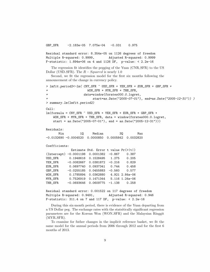
GBP_SFR -2.183e-05 7.075e-04 -0.031 0.975
Residual standard error: 8.354e-05 on 1126 degrees of freedom
Multiple R-squared: 0.9999, Adjusted R-squared: 0.9999
F-statistic: 1.894e+06 on 4 and 1126 DF, p-value: < 2.2e-16
The regression fit identifies the pegging of the Yuan (CNR SFR) to the USDollar (USD SFR). The R− Squared is nearly 1.0
Second, we fit the regression model for the first six months following theannouncement of the change in currency policy.
> lmfit.period2<-lm( CNY_SFR ~ USD_SFR + YEN_SFR + EUR_SFR + GBP_SFR +
+ WON_SFR + MYR_SFR + THB_SFR,
+ data=window(fxrates000.0.logret,
+ start=as.Date("2005-07-01"), end=as.Date("2005-12-31")) )
> summary.lm(lmfit.period2)
Call:
lm(formula = CNY_SFR ~ USD_SFR + YEN_SFR + EUR_SFR + GBP_SFR +
WON_SFR + MYR_SFR + THB_SFR, data = window(fxrates000.0.logret,
start = as.Date("2005-07-01"), end = as.Date("2005-12-31")))
Residuals:
Min 1Q Median 3Q Max
-0.0132690 -0.0004520 0.0000850 0.0005842 0.0032820
Coefficients:
Estimate Std. Error t value Pr(>|t|)
(Intercept) -0.0001198 0.0001382 -0.867 0.387
USD_SFR 0.1948616 0.1528495 1.275 0.205
YEN_SFR -0.0082667 0.0381872 -0.216 0.829
EUR_SFR 0.0697740 0.0937341 0.744 0.458
GBP_SFR -0.0255185 0.0455883 -0.560 0.577
WON_SFR 0.1785894 0.0362880 4.921 2.84e-06
MYR_SFR 0.7526919 0.1471344 5.116 1.24e-06
THB_SFR -0.0693646 0.0609775 -1.138 0.258
Residual standard error: 0.001522 on 117 degrees of freedom
Multiple R-squared: 0.9491, Adjusted R-squared: 0.946
F-statistic: 311.4 on 7 and 117 DF, p-value: < 2.2e-16
During this six-month period, there is evidence of the Yuan departing froma US Dollar peg. The exchange rates with the statsitically significant regressionparameters are for the Korean Won (WON SFR) and the Malaysian Ringgit(MYR SFR).
To examine for futher changes in the implicit reference basket, we fit thesame model for the annual periods from 2006 through 2012 and for the first 6months of 2013.
9

> for (year0 in as.character(c(2006:2013))){
+ # year0<-"2012"
+ lmfit.year0<-lm( CNY_SFR ~ USD_SFR + YEN_SFR + EUR_SFR + GBP_SFR +
+ WON_SFR + MYR_SFR + THB_SFR,
+ data=fxrates000.0.logret[year0])
+
+ cat("\n\n--------------------------------\n");cat(year0);cat(":\n")
+ print(summary.lm(lmfit.year0))
+ rate.appreciation.usd<-round( exp(252*log(1+ lmfit.year0$coefficients[1])) -1,digits=3)
+ cat("\n"); cat(year0); cat("\t Annualized appreciation rate to implied reference basket: "); cat(rate.appreciation.usd); cat("\n")
+ }
--------------------------------
2006:
Call:
lm(formula = CNY_SFR ~ USD_SFR + YEN_SFR + EUR_SFR + GBP_SFR +
WON_SFR + MYR_SFR + THB_SFR, data = fxrates000.0.logret[year0])
Residuals:
Min 1Q Median 3Q Max
-2.413e-03 -2.625e-04 5.131e-05 3.899e-04 2.504e-03
Coefficients:
Estimate Std. Error t value Pr(>|t|)
(Intercept) -1.173e-04 4.228e-05 -2.773 0.005979
USD_SFR 9.222e-01 1.859e-02 49.614 < 2e-16
YEN_SFR -5.226e-03 1.121e-02 -0.466 0.641520
EUR_SFR -1.841e-02 2.927e-02 -0.629 0.529985
GBP_SFR -1.693e-02 1.695e-02 -0.999 0.318732
WON_SFR 2.906e-02 1.201e-02 2.420 0.016245
MYR_SFR 6.909e-02 1.904e-02 3.628 0.000348
THB_SFR -8.371e-03 1.100e-02 -0.761 0.447360
Residual standard error: 0.0006512 on 243 degrees of freedom
Multiple R-squared: 0.9866, Adjusted R-squared: 0.9862
F-statistic: 2553 on 7 and 243 DF, p-value: < 2.2e-16
2006 Annualized appreciation rate to implied reference basket: -0.029
--------------------------------
2007:
Call:
10
lm(formula = CNY_SFR ~ USD_SFR + YEN_SFR + EUR_SFR + GBP_SFR +
WON_SFR + MYR_SFR + THB_SFR, data = fxrates000.0.logret[year0])
Residuals:
Min 1Q Median 3Q Max
-0.0043388 -0.0006900 0.0001165 0.0006523 0.0035492
Coefficients:
Estimate Std. Error t value Pr(>|t|)
(Intercept) -2.477e-04 7.111e-05 -3.484 0.000585
USD_SFR 9.201e-01 3.655e-02 25.172 < 2e-16
YEN_SFR -1.847e-02 1.774e-02 -1.041 0.298850
EUR_SFR 1.629e-02 4.971e-02 0.328 0.743357
GBP_SFR 4.861e-03 2.268e-02 0.214 0.830452
WON_SFR 2.148e-02 2.709e-02 0.793 0.428514
MYR_SFR 1.227e-02 2.907e-02 0.422 0.673389
THB_SFR 1.411e-03 8.770e-03 0.161 0.872287
Residual standard error: 0.001109 on 246 degrees of freedom
Multiple R-squared: 0.9332, Adjusted R-squared: 0.9313
F-statistic: 491.2 on 7 and 246 DF, p-value: < 2.2e-16
2007 Annualized appreciation rate to implied reference basket: -0.061
--------------------------------
2008:
Call:
lm(formula = CNY_SFR ~ USD_SFR + YEN_SFR + EUR_SFR + GBP_SFR +
WON_SFR + MYR_SFR + THB_SFR, data = fxrates000.0.logret[year0])
Residuals:
Min 1Q Median 3Q Max
-0.0103217 -0.0008105 0.0000162 0.0007503 0.0098093
Coefficients:
Estimate Std. Error t value Pr(>|t|)
(Intercept) -0.0002996 0.0001222 -2.452 0.01492
USD_SFR 0.9124811 0.0369556 24.691 < 2e-16
YEN_SFR -0.0010178 0.0173259 -0.059 0.95320
EUR_SFR 0.0415111 0.0342314 1.213 0.22643
GBP_SFR 0.0163507 0.0193508 0.845 0.39896
WON_SFR -0.0192298 0.0073131 -2.629 0.00909
MYR_SFR 0.0739607 0.0307166 2.408 0.01679
11

THB_SFR 0.0114822 0.0208899 0.550 0.58306
Residual standard error: 0.001906 on 244 degrees of freedom
Multiple R-squared: 0.9621, Adjusted R-squared: 0.9611
F-statistic: 885.8 on 7 and 244 DF, p-value: < 2.2e-16
2008 Annualized appreciation rate to implied reference basket: -0.073
--------------------------------
2009:
Call:
lm(formula = CNY_SFR ~ USD_SFR + YEN_SFR + EUR_SFR + GBP_SFR +
WON_SFR + MYR_SFR + THB_SFR, data = fxrates000.0.logret[year0])
Residuals:
Min 1Q Median 3Q Max
-1.994e-03 -1.400e-04 1.770e-06 1.305e-04 1.221e-03
Coefficients:
Estimate Std. Error t value Pr(>|t|)
(Intercept) 7.771e-06 2.176e-05 0.357 0.721273
USD_SFR 9.405e-01 9.676e-03 97.201 < 2e-16
YEN_SFR 5.974e-03 2.960e-03 2.018 0.044641
EUR_SFR -1.549e-02 6.958e-03 -2.227 0.026879
GBP_SFR 4.148e-03 3.014e-03 1.376 0.170055
WON_SFR -1.672e-03 2.669e-03 -0.626 0.531606
MYR_SFR 2.530e-02 6.950e-03 3.640 0.000333
THB_SFR 3.102e-02 1.239e-02 2.504 0.012946
Residual standard error: 0.0003438 on 244 degrees of freedom
Multiple R-squared: 0.9984, Adjusted R-squared: 0.9983
F-statistic: 2.165e+04 on 7 and 244 DF, p-value: < 2.2e-16
2009 Annualized appreciation rate to implied reference basket: 0.002
--------------------------------
2010:
Call:
lm(formula = CNY_SFR ~ USD_SFR + YEN_SFR + EUR_SFR + GBP_SFR +
WON_SFR + MYR_SFR + THB_SFR, data = fxrates000.0.logret[year0])
12

Residuals:
Min 1Q Median 3Q Max
-0.0051398 -0.0002402 0.0000951 0.0003745 0.0036134
Coefficients:
Estimate Std. Error t value Pr(>|t|)
(Intercept) -9.527e-05 6.374e-05 -1.495 0.1363
USD_SFR 9.116e-01 3.078e-02 29.613 <2e-16
YEN_SFR 1.170e-03 1.048e-02 0.112 0.9112
EUR_SFR 2.072e-02 1.441e-02 1.439 0.1516
GBP_SFR -3.160e-02 1.248e-02 -2.532 0.0120
WON_SFR 2.656e-03 1.066e-02 0.249 0.8035
MYR_SFR 2.359e-02 1.801e-02 1.310 0.1915
THB_SFR 6.507e-02 3.372e-02 1.930 0.0548
Residual standard error: 0.0009746 on 242 degrees of freedom
Multiple R-squared: 0.9805, Adjusted R-squared: 0.9799
F-statistic: 1739 on 7 and 242 DF, p-value: < 2.2e-16
2010 Annualized appreciation rate to implied reference basket: -0.024
--------------------------------
2011:
Call:
lm(formula = CNY_SFR ~ USD_SFR + YEN_SFR + EUR_SFR + GBP_SFR +
WON_SFR + MYR_SFR + THB_SFR, data = fxrates000.0.logret[year0])
Residuals:
Min 1Q Median 3Q Max
-0.0048725 -0.0005380 0.0000138 0.0005746 0.0061446
Coefficients:
Estimate Std. Error t value Pr(>|t|)
(Intercept) -1.968e-04 8.079e-05 -2.436 0.0156
USD_SFR 8.702e-01 2.834e-02 30.705 < 2e-16
YEN_SFR 7.857e-03 1.519e-02 0.517 0.6054
EUR_SFR -3.959e-04 1.670e-02 -0.024 0.9811
GBP_SFR 4.297e-02 2.092e-02 2.054 0.0410
WON_SFR -2.590e-02 1.696e-02 -1.527 0.1281
MYR_SFR 9.535e-02 2.351e-02 4.056 6.73e-05
THB_SFR 1.743e-02 3.329e-02 0.523 0.6011
13

Residual standard error: 0.001275 on 243 degrees of freedom
Multiple R-squared: 0.9837, Adjusted R-squared: 0.9832
F-statistic: 2097 on 7 and 243 DF, p-value: < 2.2e-16
2011 Annualized appreciation rate to implied reference basket: -0.048
--------------------------------
2012:
Call:
lm(formula = CNY_SFR ~ USD_SFR + YEN_SFR + EUR_SFR + GBP_SFR +
WON_SFR + MYR_SFR + THB_SFR, data = fxrates000.0.logret[year0])
Residuals:
Min 1Q Median 3Q Max
-0.0042900 -0.0003965 0.0000060 0.0004424 0.0044475
Coefficients:
Estimate Std. Error t value Pr(>|t|)
(Intercept) -1.951e-05 6.105e-05 -0.320 0.7495
USD_SFR 9.064e-01 2.669e-02 33.957 < 2e-16
YEN_SFR -5.759e-03 1.323e-02 -0.435 0.6637
EUR_SFR -1.320e-01 5.985e-02 -2.205 0.0284
GBP_SFR -8.758e-03 2.132e-02 -0.411 0.6816
WON_SFR 1.777e-03 2.282e-02 0.078 0.9380
MYR_SFR 1.103e-01 2.216e-02 4.979 1.21e-06
THB_SFR 1.895e-03 2.880e-02 0.066 0.9476
Residual standard error: 0.0009568 on 243 degrees of freedom
Multiple R-squared: 0.9711, Adjusted R-squared: 0.9702
F-statistic: 1165 on 7 and 243 DF, p-value: < 2.2e-16
2012 Annualized appreciation rate to implied reference basket: -0.005
--------------------------------
2013:
Call:
lm(formula = CNY_SFR ~ USD_SFR + YEN_SFR + EUR_SFR + GBP_SFR +
WON_SFR + MYR_SFR + THB_SFR, data = fxrates000.0.logret[year0])
Residuals:
14
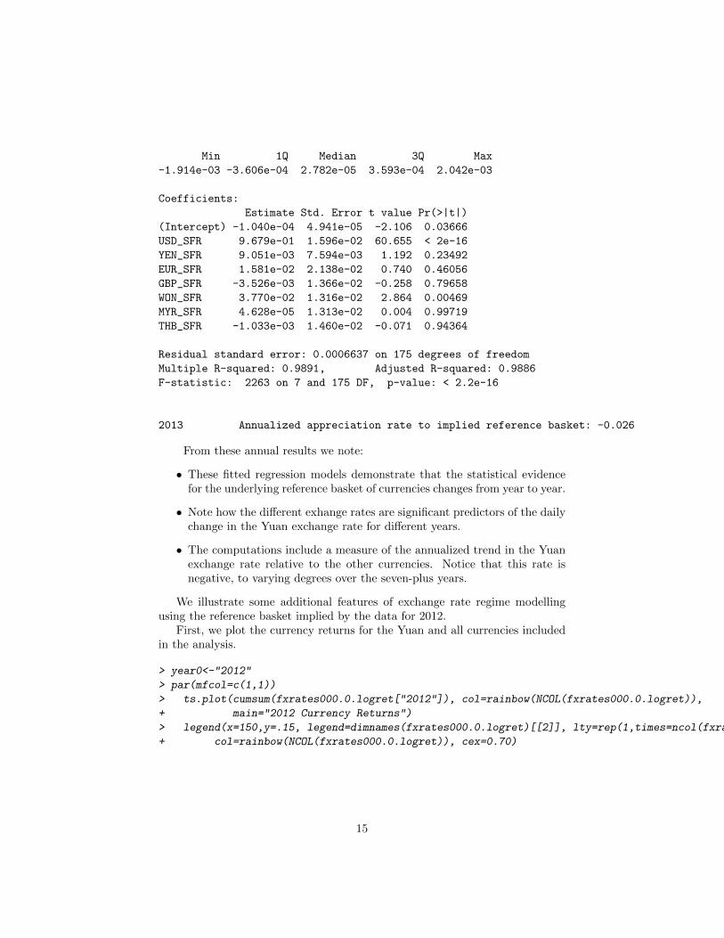
Min 1Q Median 3Q Max
-1.914e-03 -3.606e-04 2.782e-05 3.593e-04 2.042e-03
Coefficients:
Estimate Std. Error t value Pr(>|t|)
(Intercept) -1.040e-04 4.941e-05 -2.106 0.03666
USD_SFR 9.679e-01 1.596e-02 60.655 < 2e-16
YEN_SFR 9.051e-03 7.594e-03 1.192 0.23492
EUR_SFR 1.581e-02 2.138e-02 0.740 0.46056
GBP_SFR -3.526e-03 1.366e-02 -0.258 0.79658
WON_SFR 3.770e-02 1.316e-02 2.864 0.00469
MYR_SFR 4.628e-05 1.313e-02 0.004 0.99719
THB_SFR -1.033e-03 1.460e-02 -0.071 0.94364
Residual standard error: 0.0006637 on 175 degrees of freedom
Multiple R-squared: 0.9891, Adjusted R-squared: 0.9886
F-statistic: 2263 on 7 and 175 DF, p-value: < 2.2e-16
2013 Annualized appreciation rate to implied reference basket: -0.026
From these annual results we note:
• These fitted regression models demonstrate that the statistical evidencefor the underlying reference basket of currencies changes from year to year.
• Note how the different exhange rates are significant predictors of the dailychange in the Yuan exchange rate for different years.
• The computations include a measure of the annualized trend in the Yuanexchange rate relative to the other currencies. Notice that this rate isnegative, to varying degrees over the seven-plus years.
We illustrate some additional features of exchange rate regime modellingusing the reference basket implied by the data for 2012.
First, we plot the currency returns for the Yuan and all currencies includedin the analysis.
> year0<-"2012"
> par(mfcol=c(1,1))
> ts.plot(cumsum(fxrates000.0.logret["2012"]), col=rainbow(NCOL(fxrates000.0.logret)),
+ main="2012 Currency Returns")
> legend(x=150,y=.15, legend=dimnames(fxrates000.0.logret)[[2]], lty=rep(1,times=ncol(fxrates000.0.logret)),
+ col=rainbow(NCOL(fxrates000.0.logret)), cex=0.70)
15

2012 Currency Returns
Time
0 50 100 150 200 250
−0.
050.
000.
050.
100.
15CNY_SFRYEN_SFRWON_SFRMYR_SFREUR_SFRGBP_SFRTHB_SFRUSD_SFR
Then, we plot the currency return of the Yuan and that of the impliedreference basket specified by the regression:
> lmfit.year0<-lm( CNY_SFR ~ USD_SFR + YEN_SFR + EUR_SFR + GBP_SFR +
+ WON_SFR + MYR_SFR + THB_SFR,
+ data=fxrates000.0.logret[year0])
> y0.actual<-fxrates000.0.logret["2012"][,"CNY_SFR"]
> y0.fit<-y0.actual - lmfit.year0$residuals
> ts.plot(cumsum(cbind(y0.actual, y0.fit)),
+ col=rainbow(NCOL(fxrates000.0.logret))[c(1,5)],
+ main="2012 Currency Returns \nCNY_SFR and Implied Basket")
16

2012 Currency Returns CNY_SFR and Implied Basket
Time
0 50 100 150 200 250
−0.
06−
0.04
−0.
020.
000.
020.
04
Note how closely the reference basket tracks the Yuan. This is to beexpected given the high R−squared of the regression.
Finally, we apply the R function influence.measures()
> layout(matrix(c(1,2,3,4),2,2)) # optional 4 graphs/page
> plot(lmfit.year0)
17

−0.02 −0.01 0.00 0.01 0.02
−0.
004
0.00
00.
004
Fitted values
Res
idua
ls
Residuals vs Fitted
2012−05−01
2012−03−222012−04−30
−3 −2 −1 0 1 2 3
−4
02
4
Theoretical Quantiles
Sta
ndar
dize
d re
sidu
als
Normal Q−Q
2012−05−01
2012−03−222012−04−30
−0.02 −0.01 0.00 0.01 0.02
0.0
0.5
1.0
1.5
2.0
Fitted values
Sta
ndar
dize
d re
sidu
als
Scale−Location2012−05−012012−03−222012−04−30
0.00 0.05 0.10 0.15
−4
02
4
Leverage
Sta
ndar
dize
d re
sidu
als
Cook's distance1
0.5
0.5
1Residuals vs Leverage
2012−03−222012−04−30
2012−01−31
These diagnostics indicate:
• The residuals appear well-behaved as they relate to the size of the fittedvalues. The residual variance does not increase with the magnitude of thefitted values.
• The residuals exhibit heavier tails than those of a normal distribution.However for those residuals within two standard deviations of their mean,their distribution is close to that of a normal distribution.
18
References
Frankel J.A., and S Wei (1994) Yen Bloc or Dollar Bloc? Exchange RatePolicies of the East Asian Economies, Chaptr in Macroeconomic Link-age: Savings, Exchange Rates, and Capital Flows, NBER-EASE Volume3, Takatoshi Ito and Anne Krueger, editors. University of Chicago Press,Chapter URL: http://www.nber.org/chapters/c8537.pdf
Frankel J.A., and S Wei (2007) Assessing China’s Exchange Rate Regime,
NATIONAL BUREAU OF ECONOMIC RESEARCH: Working Paper13100, http://www.nber.org/papers/w13100 , Cambridge.
19

MIT OpenCourseWarehttp://ocw.mit.edu
18.S096 Topics in Mathematics with Applications in FinanceFall 2013
For information about citing these materials or our Terms of Use, visit: http://ocw.mit.edu/terms.
Top Related