


Languages
Pages
Legal

Optimisation of Process Parameters in ECM
by using Rotary U Shaped Tool
Rahul Ganjir
(209ME2198)
Department of Mechanical Engineering
National Institute of Technology Rourkela
Rourkela-769 008, Orissa, India
May 2010
Optimisation of Process Parameters in ECM
by using Rotary U Shaped Tool
Thesis submitted in partial fulfilment
of the requirements for the degree of
Master of Technology
in
Mechanical Engineering
by
Rahul Ganjir
(209ME2198)
under the supervision of
Prof. C. K. Biswas
Department of Mechanical Engineering
National Institute of Technology Rourkela
Rourkela-769 008, Orissa, India
May 2010
ii
Certificate
This is to certify that thesis entitled, “Optimisation of Process Parameters in ECM by
using Rotary U Shaped Tool” submitted by Mr. Rahul Ganjir in partial fulfillment of
the requirements for the award of Master of Technology in Mechanical Engineering with
“Production Engineering” Specialization during session 2009-2011 in the Department of
Mechanical Engineering National Institute of Technology, Rourkela. It is an authentic work
carried out by him under my supervision and guidance. To the best of my knowledge, the
matter embodied in this thesis has not been submitted to any other University/Institute
for award of any Degree or Diploma.
Dr. C. K. Biswas
Associate Professor
Place Department of Mechanical Engineering
Date National institute of technology, Rourkela
Department of Mechanical Engineering
National Institute of Technology Rourkela
Rourkela-769 008, Orissa, India

iii
Acknowledgement
I express my deep sense of gratitude and indebtedness to my thesis supervisor Dr. C. K.
Biswas, Associate Professor, Department of Mechanical Engineering for providing precious
guidance, inspiring discussions and constant supervision throughout the course of this work.
His timely help, constructive criticism, and conscientious efforts made it possible to present
the work contained in this thesis.
I express my sincere thanks to Mr. Shailesh Kumar Dewangan, Research Scholar and Mr.
A. Prabhakar. I am grateful to Prof. R. K. Sahoo, Head of the Department of Mechanical
Engineering for providing me the necessary facilities in the department. I express my sincere
gratitude to Prof. S. S. Mahapatra, coordinator of Mechanical Engineering course for his
timely help during the course of work. I am also thankful to all the staff members of the
department of Mechanical Engineering and to all my well-wishers for their inspiration and
help. And also to thanks my classmate’s Mr. Kamal Kumar Kanujia during the help my
project.
I feel pleased and privileged to fulfill my parent’s ambition and I am greatly indebted to
them for bearing the inconvenience during my M Tech. course.
Rahul Ganjir
iv
Abstract
Electrochemical machining (ECM) has established itself as one of the major
alternatives to conventional methods for machining hard materials and complex contours
without the residual stresses and tool wear. ECM has extensive application in automotive,
petroleum, aerospace, textile, medical and electronic industries. Studies on Material Removal
Rate (MRR) are of utmost importance in ECM, since it is one of the determining factors in
the process decisions. So the aim of present work is to investigate the MRR, overcut
diameter and overcut depth of AISI P20 work piece by using a rotating copper U-tube tool.
Four parameters were chosen as process variables: Feed rate, Voltage, Electrolyte
concentration and Tool diameter.
The results of experiment show the material removal increase with increasing the
feed, voltage and electrolyte concentration but decreases with increasing the tool diameter,
and for both overcut diameter and overcut depth they increases with increasing feed ,voltage
and electrode diameter but decreases with increasing electrolyte concentration. Grey relation
grade (GRD) was also applied to identify the optimal parameter setting in the experiment.
Keywords: Electrochemical Machining (ECM), Taguchi Method, Metal Removal Rate
(MRR), Overcut (OC), Grey Relation Analysis (GRA).
v
Contents Page No.
Certificate…………………………………………………………………………….. ii
Acknowledgement……………………………………………………………………. iii
Abstract………………………………………………………………………………. iv
List of Figures………………………………………………………………………... vii
List of Tables…………………………………………………………………………. viii
1. Introduction 1
1.1 Fundamental Principle……………………………………………………. 1
1.2 ECM Machine Parameters………………………………………………... 2
1.2.1 Servo System……………………………………………………... 2
1.2.2 Electrolyte………………………………………………………... 3
1.2.3 Tool Feed Rate…………………………………………………… 4
1.2.4 Material Removal Rate…………………………………………… 4
1.2.5 Tool Design………………………………………………………. 4
1.2.6 Pumps……………………………………………………………. 5
1.2.7 Filtration and Storage Tank………………………………………. 5
1.2.8 Valves and Piping………………………………………………… 5
1.3 Thesis Organization………………………………………………………. 5
2. Literature Survey 6
2.1 Overview based on tool design on ECM…………………………………. 6
2.2 Overview based on surface finish on ECM………………………………. 8
2.3 Overview based on electrolyte concentration on ECM………………….. 12
2.4 Conclusion and Research Objectives………………………………….. 15
3. Experimental setup and Tool design 17
3.1 Experimental Objectives…………………………………………………. 17
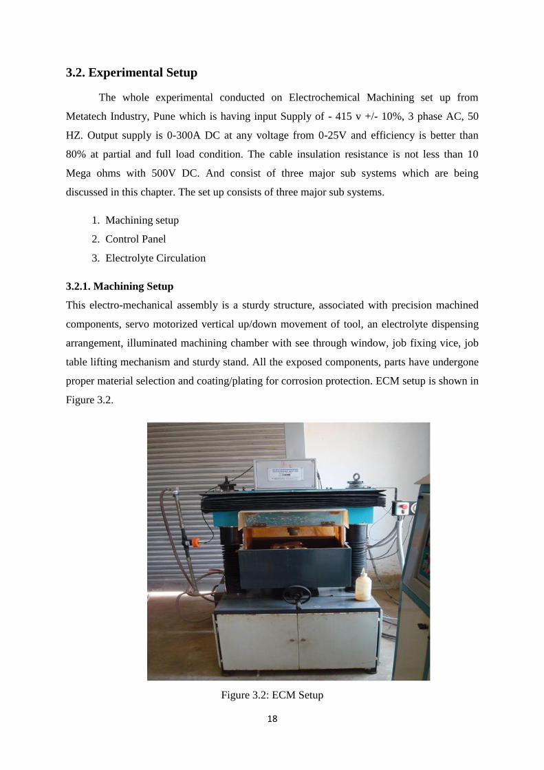
3.2 Experimental Setup………………………………………………………. 18
3.2.1 Machining Setup…………………………………………………. 18
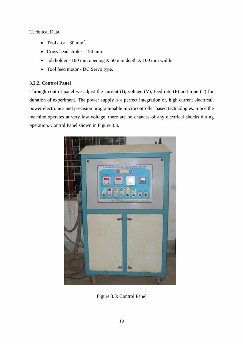
3.2.2 Control Panel…………………………………………………….. 19
3.2.3 Electrolyte Circulation…………………………………………… 20
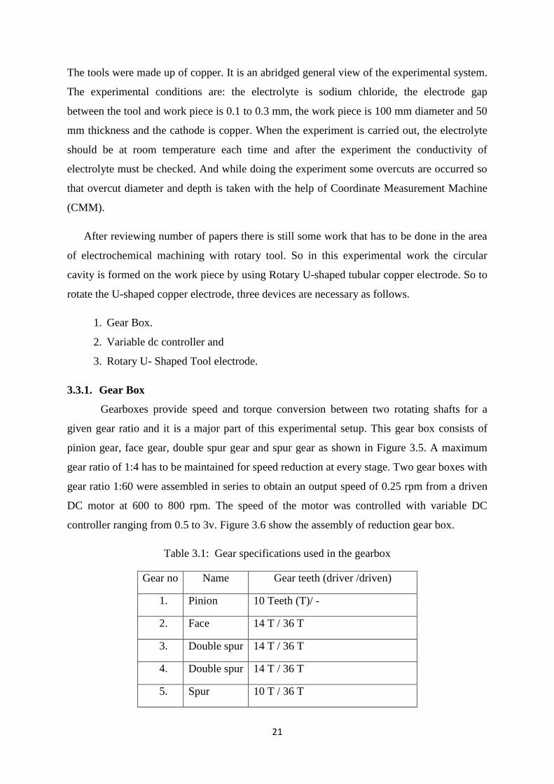
3.3. Tool Setup…………………………………………………………………. 20
3.3.1 Gear Box…………………………………………………………... 21

vi
3.3.2 Variable DC Power Controller…………………………………….. 22
3.3.3 Rotary U-Shaped tool electrode…………………………………. 24
3.4. Conclusion………………………………………………………………… 27
4. Experimental Work 28
4.1 Specification of Work-piece material……………………………………… 28
4.2 Taguchi Experimental Design and Analysis………………………………. 29
4.2.1 Taguchi’s Philosophy……………………………………………… 29
4.2.2 Experimental Design Strategy…………………………………….. 29
4.3 Making of Brine Solution………………………………………………….. 30
4.4 Experimental Procedure……………………………………………………. 31
4.5 Sample Calculation (For run order 1)……………………………………… 35
4.6 Grey relation analysis……………………………………………………… 35
4.7.1 Grey relation generation…………………………………………… 35
4.7.2 Grey relation coefficient…………………………………………… 36
4.7.3 Grey relation grade………………………………………………. 36
4.8. Conclusion………………………………………………………………… 38
5. Result and Discussion 39
5.1 Analysis of Experiment and Discussions………………………………….. 39
5.1.1 Effect on MRR…………………………………………………….. 39
5.1.2 Effect on OC-diameter…………………………………………….. 42
5.1.3 Effect on OC-depth………………………………………………... 46
5.2 Conclusion…………………………………………………………………. 49
6. Conclusion 50
References 51
Dissemination of Work 54

vii
List of Figures Page No.
Figure 1.1: Principle of Electrochemical Machining………………………………… 2
Figure 1.2: Overall concepts and calculation methods for potentials………………... 3
Figure 3.1: Schematic diagram of ECM……………………………………………... 17
Figure 3.2: ECM Setup………………………………………………………………. 18
Figure 3.3: Control Panel…………………………………………………………….. 19
Figure 3.4 Electrolyte tank with Filter……………………………………………….. 20
Figure 3.5: Gear Box…………………………………………………………………. 22
Figure 3.6 Reduction Gear box………………………………………………………. 22
Figure 3.7: Variable DC controller…………………………………………………... 23
Figure 3.8: Circuit diagram of Variable DC Power supply………………………….. 23
Figure 3.9 U-shaped Copper Tube…………………………………………………… 24
Figure 3.10: Tool Holder…………………………………………………………….. 25
Figure 3.11: Rotary U-shaped Tool assembly………………………………………... 25
Figure 3.12: Schematic diagram of Rotary Tool……………………………………... 26
Figure 3.13: Gear arrangement with Rotary Tool……………………………………. 26
Figure 4.1: Machining step 1………………………………………………………… 31
Figure 4.2: After Machining in step 2………………………………………………... 32
Figure 4.3: Work-piece after machining (number inscribed represents run order)…... 32
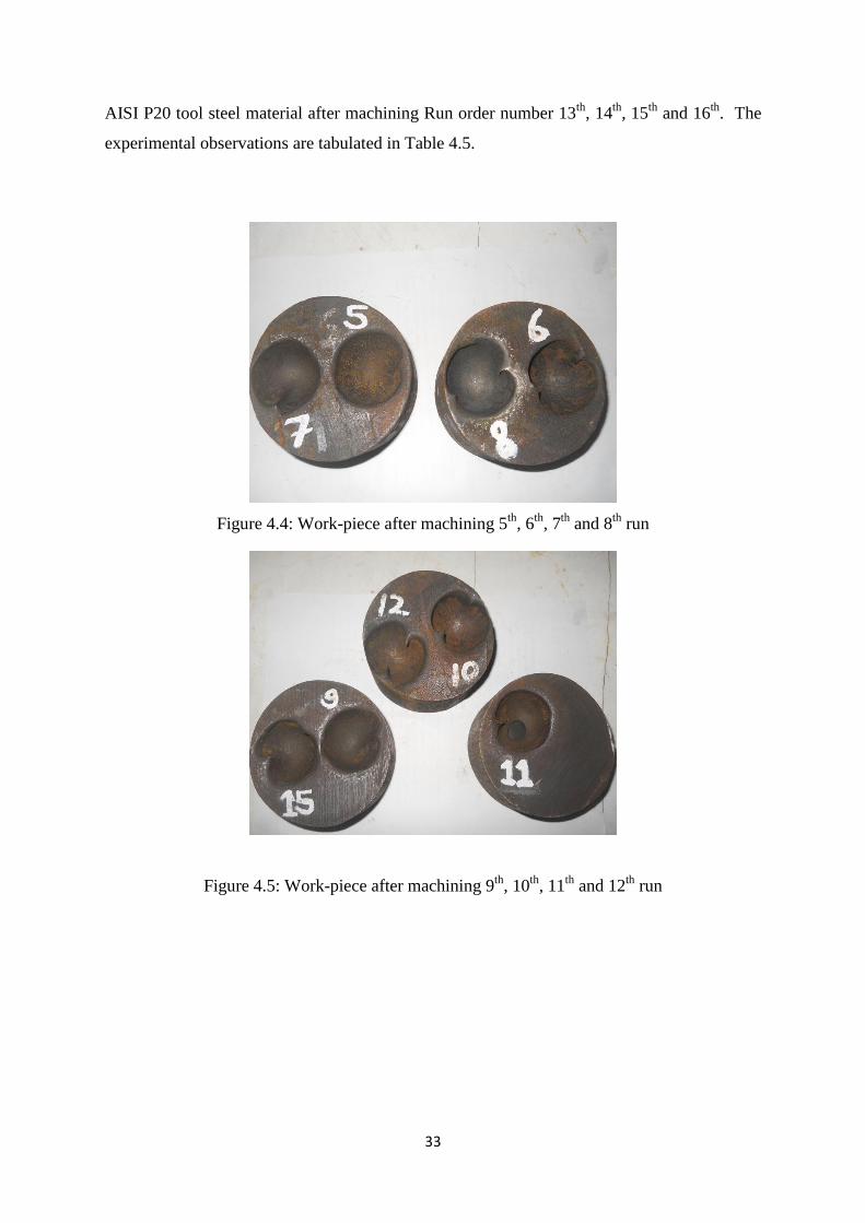
Figure 4.4: Work-piece after machining 5th, 6th, 7th and 8th run …………………... 33
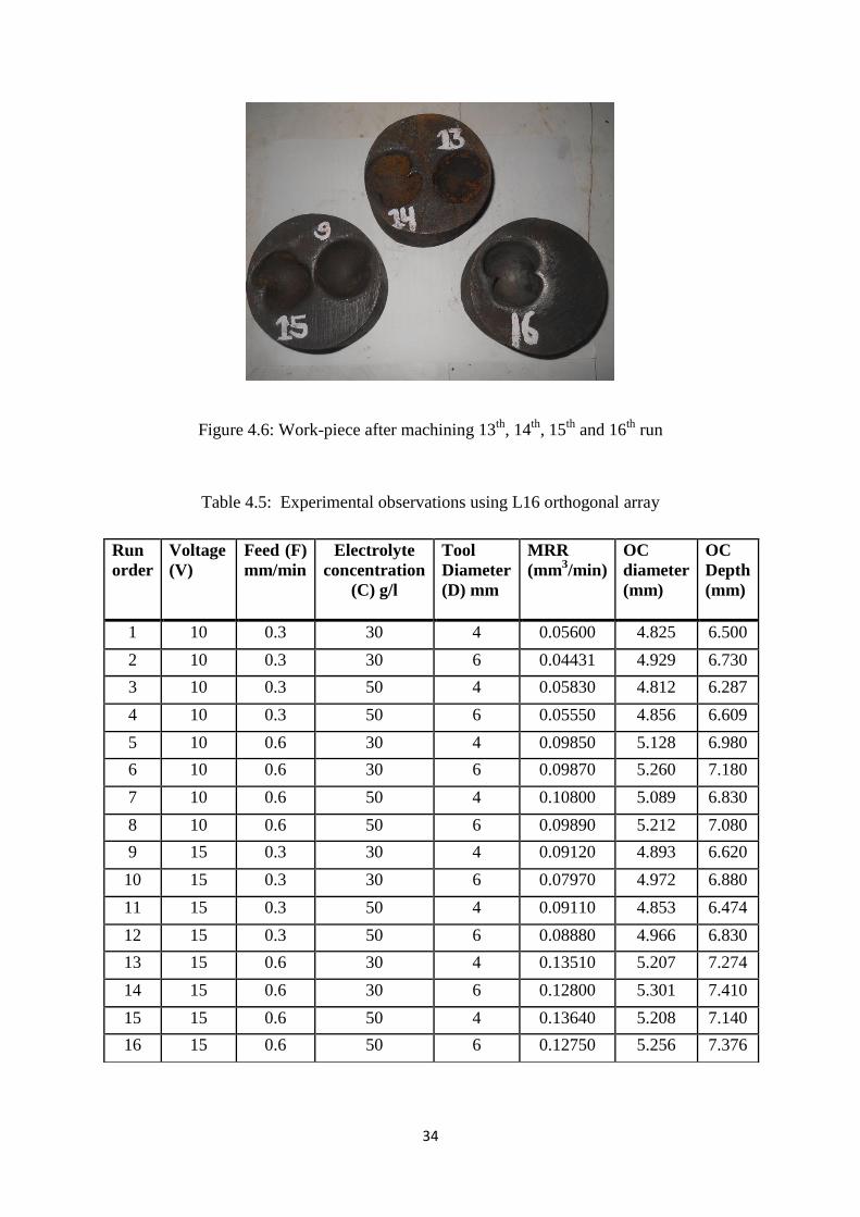
Figure 4.5: Work-piece after machining 9th, 10th, 11th and 12th run ………………. 33
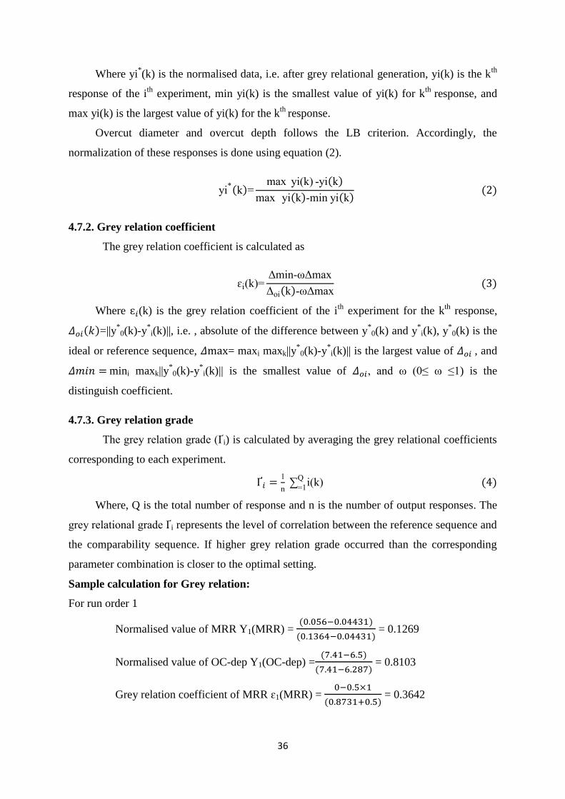
Figure 4.6: Work-piece after machining for 13th, 14th, 15th and 16th run …………. 34
Figure 4.7: Grey Relation Grade……………………………………………………... 38
Figure5.1: Main effect Plot for MRR………………………………………………… 39
Figure5.2: Residual Plots for MRR…………………………………………………... 42
Figure5.3 Main effect Plot for OC-diameter…………………………………………. 43
Figure5.4: Residual Plots for OC-diameter…………………………………………... 45
Figure5.5: Main effect Plot for OC-depth……………………………………………. 46
Figure5.6: Residual Plots for OC-depth……………………………………………… 48
viii
List of Tables Page No.
Table 3.1: Gear specification used in gearbox……………………………………….. 21
Table 4.1: Description of AISI P20 steel…………………………………………….. 28
Table 4.2: Work piece Composition…………………………………………………. 28
Table 4.3: Mechanical and Thermal Properties……………………………………… 28
Table 4.4: Machining parameters and there levels…………………………………… 30
Table 4.5: Experimental observations using L16 orthogonal array………………….. 34
Table 4.6: Evaluated grey relational grade for responses……………………………. 37
Table 5.1: ANOVA for MRR………………………………………………………… 40
Table 5.2: ANOVA for MRR after eliminating non-significant values……………… 40
Table 5.3: Taguchi analysis response table for MRR………………………………... 41
Table 5.4: Estimated Model Coefficient for Means of MRR………………………… 41
Table 5.5: ANOVA for OC-diameter………………………………………………… 43
Table 5.6: ANOVA for OC-diameter after eliminating non-significant values……… 44
Table 5.7: Taguchi analysis response table for OC-diameter………………………... 44
Table 5.8: Estimated Model Coefficient for Means of OC-diameter………………… 45
Table 5.9: ANOVA for OC-depth……………………………………………………. 47
Table 5.10: ANOVA for OC-depth after eliminating non-significant values……….. 47
Table 5.11: Taguchi analysis response table for OC-depth………………………….. 47
Table 5.12: Estimated Model Coefficient for Means of OC-depth…………………. 48

1
Chapter 1
Introduction
Electrochemical machining (ECM) was developed to machine difficult-to cut materials, and it
is an anodic dissolution process based on the phenomenon of electrolysis, whose laws were
established by Michael Faraday [1]. In ECM, electrolytes serve as conductors of electricity.
The rate of machining does not depend on the hardness of the metal. ECM offers a number of
advantages over other machining methods and also has several disadvantages:
Advantages: there is no tool wear; machining is done at low voltage compared to
other processes with high metal removal rate; no burr formation; hard conductive materials
can be machined into complicated profiles; work-piece structure suffer no thermal damages;
suitable for mass production work and low labour requirements.
Disadvantages: a huge amount of energy is consumed that is approximately 100 times
that required for the turning or drilling of steel; safety issues on removing and disposing of
the explosive hydrogen gas generated during machining; not suited for nonconductive
materials and difficulty in handling and containing the electrolyte [2].
Applications: ECM is widely used in manufacturing for making moulds and dies; also
used for making complicated shape of turbine blades and it is now routinely used for the
machining of aerospace components, critical deburring, Fuel injection system components,
ordnance components etc.
As shown in Figure 1.1, the shaped tool (cathode) is connected to the negative
polarity and the work-piece (anode) is connected to the positive polarity. The electrolyte flow
through the small inter-electrode gap, thus flushing away sludge and heat generated during
machining process.
1.1. Fundamental Principles
During ECM, there will be reactions occurring at the electrodes i.e. at the anode or work-
piece and at the cathode or the tool along with within the electrolyte. Ion and electrons
crossing phase boundaries (the interface between two or more separate phases, such as liquid-
solid) would result in electron transfer reaction carried out at both anode and cathode.

2
Figure 1.1: Principle of Electrochemical Machining
Meanwhile, the potential difference is fundamental in understanding the energy
distribution during the electrochemical machining process. Figure 1.2 shows the broad
concepts and basic potential calculation methods. Nernst equation is used to calculate the
electrode reversible potential. Tafel equation, diffusion layer, and ohm’s law can assist in
estimating activation overpotential, concentration overpotential, and resistance overpotential,
which are known as the three main overpotentials in electrochemical reactions.
1.2. ECM Machine Parameters: 1.2.1. Servo System:
The servo system controls the tool motion relative to the work piece to follow the
desired path. It also controls the gap width within such a range that the discharge process can
continue. If tool electrode moves too fast and touches the work piece, short circuit
occurs. Short circuit contributes little to material removal because the voltage drop
between electrodes is small and the current is limited by the generator. If tool electrode
moves too slowly, the gap becomes too wide and electrical discharge never occurs. Another
function of servo system is to retract the tool electrode when deterioration of gap condition is

3
Figure 1.2 Overall concepts and calculation methods for potentials
Detected. The width cannot be measured during machining; other measurable variables are
required for servo control.
1.2.2. Electrolyte:
The electrolyte is essential for the electrolytic process to work. The electrolyte has three
main functions in ECM. These three functions are:
1. It carries the current between the tool and the work-piece.
2. It removes the products of machining from the cutting region.
3. It dissipates heat produced in the operation.
Electrolytes must have high electrical conductivity, low toxicity and low corrosiveness.
The electrolyte is pumped at about 14 kg/cm2 and at speed of at least 30 m/s.
4
1.2.3. Tool Feed Rate:
In ECM process gap about 0.01 to 0.07 mm is maintained between tool and
work piece. For smaller gap, the electrical resistance between the tool and work is
least and the current is maximum and accordingly maximum metal is removed. The
tool is feed in to the work depending upon the how fast the metal is to be removed.
The movement of the tool slide is controlled by a hydraulic cylinder giving some range of
feed rate.
1.2.4. Material Removal Rate:
It is a function of feed rate which dictates the current passed between the work and the
tool. As the tool advances towards work, gap decreases and current increases which increases
more metal at a rate corresponding to tool advance. A stable spacing between tool and work
is thus established. It may be noted that high feed rate not only is productive but also
produces best quality of surface finish. However feed rate is limited by removal of hydrogen
gas and products of machining. Metal removal rate is lower with low voltage, low electrolyte
concentration and low temperature.
The primary advantages of the metal removal rate process are that they do not cause
certain undesirable surface effects which occurred in conventional machines. The main
advantages are that they are stress free machining, burr free surfaces, reduced tool wear and
elimination of thermal damage to the work-piece. These processes have no effect on
mechanical properties such as yield strength, ultimate tensile strength, ductility, hardness etc.
1.2.5. Tool Design:
As no tool wear takes place, any good conductor is satisfactory as a tool material, but
it must be designed strong enough to withstand the hydrostatic force, caused by electrolyte
being forced at high speed through the gap between tool and work. The tool is made hollow
for drilling holes so that electrolyte can pass along the bore in tool. Cavitation, stagnation and
vortex formation in electrolyte flow must be avoided because these result a poor surface
finish. It should be given such a shape that the desired shape of job is achieved for the given
machining condition.
Both external and internal geometries can be machined with an electrochemical
machine. Copper is often used as the electrode material. Brass, graphite, and copper-tungsten
are also often used because of the ability to be easily machined, they are conductive
materials, and they will not corrode.
5
There are two major aspects of tool design. These are:
1. Determining the tool shape so that the desired shape of the job is achieved for the
given machining conditions.
2. Designing the tool for considerations other than e.g. electrolyte flow, insulation,
strength and fixing arrangements.
1.2.6. Pumps:
Single or multi-stage centrifugal pumps are used on ECM equipment. A minimum
flow rate 15 litres/min per 1000 A. Electrolyzing current is generally required. A pressure of
5-30 kg/cm2 meets most of the requirements of ECM application.
1.2.7. Filtration and Storage Tank:
The filtration of electrolyte is essential to prevent small particles of grit, metal,
plastics and products of machining from entering the machining gap and causing interference
in the process, for these a 5 micron polypropylene pleated filter cartridge have been used with
stainless steel housing arrangement . These filters get clogged and need cleaning once in 30
hrs.
1.2.8. Valves and Piping:
The piping and control valves which supply electrolyte to the ECM tooling, must not
introduce foreign matter into the electrolyte. Stainless steel is the most suitable material for
valves and piping. Materials such as fibre glass and reinforced plastics are used with some
degree of success.
1.3. Thesis Organization
The rest of the thesis is organized as follows.
Chapter 2 consists of a literature review based on the ECM tool design, ECM surface
finish and review based on the effect of electrolyte concentration on response.
Chapter 3 present the experimental setup and tool design.
Chapter 4 present the result and discussion i.e. which process parameter effect more
to MRR, overcut diameter and overcut depth.
Chapter 5 makes the conclusions and offers recommendations into future research.
6
Chapter 2
Literature Survey
In this chapter, we broadly classify all the research paper into three different
categories, i.e. paper related to tool design, related to surface finish and some paper related to
type of electrolyte used.
2.1. Overview based on tool design on ECM
D. Zhu et al. [3] proposes a finite element approach to accurately determine the electrode
profiles. The proposed method does not require Iterative redesign process, therefore provides
excellent convergence and efficient computing. Tool design In ECM mainly deals with
predicting gap distribution for a given work-piece shape. Accurate design of tool shape is
decisive to machining accuracy. In this paper experiment were conducted with 150 g/l of
electrolyte ( ) and the anode is low carbon steel. In ECM experiment, an average
deviation of less than 4% between experimental and theoretical results has been observed.
Yuming Zhou et al. [4] suggest a new approach for the problem like limited applicability,
inaccuracy, and non-convergence occurred when tool (cathode) design in electrochemical
machining has been overcomes by employing a finite element method with an optimization
formulation. With the flexibility of the finite element method, even cathodes with corners,
edges and cusps could be designed, provided that suitable representations are employed.
Overall, the approach put forth here holds great promise for practical tool design in
electrochemical machining processes.
C. S. Chang et al. [5] presented the effect of thermal fluid properties in the numerical
simulation of the tool shape for given work-piece shape in electrochemical machining. A
bubbly two-phase, one-dimensional flow model and a one-phase, two-dimensional flow
model are applied to predict the fluid field of the electrolyte, respectively. Results show that
the void fraction is the most important factor in determining the electrolyte conductivity and
the shape of the work-piece. The effect of the thermal-fluid properties should be considered
in the inverse problem and the relative error of corresponding work-piece can be reduced to
about 0.002 when proper machining condition are chosen.
7
S. J. Ebeid et al. [6] studied the improvement of machining accuracy in ECM by hybridizing
the process by low-frequency vibrations. The study highlights the development of
mathematical models for correlating the inter relationships of various machining parameters
such as applied voltage, feed rate, back pressure and vibration amplitude on overcut and
conicity for achieving high controlled accuracy. This work is based on response surface
methodology (RSM) approach. Hybridization techniques are applied to ECM to improve its
performance. The present work addresses the improvement of machining accuracy in ECM
by hybridizing the process by low-frequency vibrations. The object of the tool vibrations
during the ECM process is to provide a new and improved method for ECM which:
1. Destroys the passivation layer and thereby controls the ECM action;
2. Utilizes a reciprocal motion between the tool and work-piece to pump and
consequently enhance the circulation of the electrolyte through the interface to
permit the use of high current densities in order to improve the quality of the
machined surface.
The response surface methodology used in the present work has proved its adequacy
to be an effective tool for the analysis of the ECM process and the amplitude of the tool
vibration is the most effective parameter affecting ECM accuracy. However, this effect
diminishes after the tool amplitude reaches 80 µm.
P. S. Pa [7] studied the most effective geometry for the design electrode in electrochemical
smoothing following end turning is investigated. Through simple equipment attachment,
electrochemical smoothing can follow the cutting on the same machine. When adequate
work-piece rotational speed associated with higher electrode rotation produces better
polishing. The electrode of the partial curve with a small line diameter performs the best for
the electropolishing. Electrochemical smoothing saves the need for precise turning, making
the total process time less than the electrobrightening. But the electrobrightening after precise
turning only requires quite a short time to make the work-piece bright. The use of ultrasonic
in the electrochemical smoothing and the electrobrightening is more evident than the pulsed
current, since the ultrasonic-aided process exempts off time and obtains a better polishing
result.
Chunhua Sun et al. [8] proposes an approach using finite element method (FEM) to design
tool in ECM. It is capable to design three dimensional freeform surface tool form the scanned
data of known work-piece. In the present work, he developed a technique that is capable of
8
handling three-dimensional tool design based on the Laplace’s equation of the practical
potential field with the FEM. The proposed method can deal with the three dimensional tool
design and has high computing efficiency, good accuracy and flexible boundary treatment. It
combines tool design in ECM with the technology of CAD/CAM and makes ECM tool
design procedure relatively inexpensive within shorter lead time.
J. A. Westley et al. [9] presented a paper to studied electrolyte flow, the problems occurring
during development and to derive generic design solutions arising. In addition, it was
required to identify factors, such as insulation requirements and machined face considerations
that could relate to other ECM components. The main considerations for ECM tooling are the
flow of the electrolyte solution. If the electrolyte is restricted as it exits from the flow slot,
there is a very high risk of a spark occurring between the electrode and the workface. The
results shows some point to be consider when ECM tool design these are the path of
electrolyte flow should be as unrestricted as possible, electrolyte exit slots should be of a
continuous from without V-slots or enlargements and interior of the electrolyte exit slot
should be as flat as possible.
Amalnik and McGeough [10] has reported that an intelligent knowledge-based system
(IKBS) for evaluating electrochemical machining, in a concurrent engineering (CE)
environment and based on object oriented techniques, is introduced. The design specification
is acquired through a feature-based approach. Ten different classes of design features are
interactively obtained. The attributes of 72 work piece material types, eight tool-electrode
metals, two electrolyte solutions, and seven different sizes and types of electrochemical
machines are stored in a database. For each design feature, information needed in
manufacturing, such as the machining cycle time and cost, penetration rate, efficiency and
effectiveness, costs for electricity consumed, machine installation and depreciation are
estimated. Finally, for the same design specification, machining times are compared and
ordered, for alternative unconventional processes of electrochemical, electro-discharge and
electrochemical arc machining.
2.2. Overview based on surface finish on ECM process
K. P. Rajurkar and M. S. Hewidy [11] presented a paper to examine two aspects of ECM
performance. The reduction in the experimentally measured values of the final gap with the
increase in work specimen grain size is used to develop a correction factor. The prediction of
9
the anode profile based on the correction factor and the improved cosθ method compares well
with the anode cavity profile measured with a specially designed and built instrument. The
result found that the final inter-electrode gap, the current, the machining rate, and surface
roughness are influenced by the grain size. An experimentally measured set of the final gap
values are used in conjunction with the improved cosθ method to predict the anode shape for
work-pieces of different grain size. The surface profiles have been modelled and analysed by
a stochastic methodology called Data Dependent Systems (DDS) for wavelength
decomposition. The Green's function of the ECM surface profiles is correlated with the
distribution of potential gradient or current over the work-piece surface profile.
K. P. Rajurkar et al. [12] focus on minimizing the material to be removed by predicting
minimum machining allowance and improving the degree of localized dissolution. the anode
dissolution should be maximum at higher current densities and almost zero at lower current
densities. The results suggest the effectiveness of using proper short pulse to achieve a higher
degree of localized dissolution. It is found that pulse ECM with an on-time of 1-3ms and a
duty factor of 50% provides optimum estimates for desired dimensional accuracy. The
passivating electrolyte such as exhibits better machinability characteristics.
Approximately 35% reduction in material to be removed is estimated by the use of PECM
with electrolyte.
M. S. Hewidy [13] developed new technique to utilize a simultaneously moving and rotating
electrode to remove a specific amount of material from pre-machined holes and rods of
hardened steel specimens. One of the electrodes was provided with two simultaneous
movements, traverse speed and rotational speed. Experimental results revealed that this
technique could lead to the removal of a surface layer thickness up to 200µ, which
consequently classified this method as a super-finishing process, shows the machining cell
that has been used for hole and rod finishing. The cell has been adapted to work on a radial
drilling machine to get the advantages of the controlled feed rate and the rotational motion of
the tool. The electrolyte was sodium chloride (200 g/l), and has been fed into the cell through
a centrifugal pump drawing from a plastic tank (1 ). In the present work, the possibility of
increasing feed rates has been achieved which could lead to the removal of wall thickness up
to 0.02 mm. This enhances the controllability of the ECM process. Theoretical model and
computer calculations facilitate the prediction of metal removal thickness through different
combinations of ECM parameters.
10
I. Strode and M. B. Bassett [14] investigated the effect of Electrochemical machining on the
surface integrity of cast and wrought steels. It is shown that the resulting surface structure and
surface finish are strongly dependent on the current density used during machining, it’s also
indicate that the surface damage resulting from electrochemical machining is less than that
obtained after electro discharge machining. The result shows some points i.e. all pre-existing
surface stresses are removed during ECM, resulting in a near-stress-free surface, the
reduction in fatigue strength which occurs after ECM at an adequate current density is mainly
due to the removal of compressive stresses and the fatigue strength of electrochemically
machined surfaces may be substantially increased by light shot peening.
Ming-Chang Jeng et al. [15] studied the effects of carbon content, microstructure and
working pressure on the metal removal rate and current efficiency in electrochemical
machining of carbon steels. In this paper four different carbon contents and various heat-
treatment procedures (quenching, tempering and annealing) were performed. The result
shows following points:
The removal rate and current efficiency increase with carbon content,
The quenched microstructure and the tempered microstructure have a greater
removal rate and current efficiency than those of annealed microstructures,
The work-piece machined at a working pressure of 3-4 kg/cm2 has the greatest
removal rate and current efficiency,
The roughness of the machined surface of the annealed microstructure is greater than
those of the quenched and tempered steels.
S. C. Tam and N.H. Loh [16] studied the ECM–abrasive polishing of mild steel specimens
using response surface methodology (RSM). Three independent parameters: ECM voltage,
electrolyte concentration and tool-holding pressure were chosen as the process variables,
whilst the surface roughness of the finished specimens, was the response variable that
had to be minimised. A minimum value of of 0.64 µm was predicted at an ECM-voltage
of 5.64 V, an electrolyte concentration of 7%, and a tool-holding pressure of 0.61 bars. There
are many process variables that can affect the surface finish of the ECM-abrasive polished
specimens: tool spindle speed, work-piece speed, oscillation frequency, tool-holding
pressure, type of abrasive, grit size, grit concentration, bond strength, electrode material, tool
gap, type of electrolyte, concentration of electrolyte, flow rate of electrolyte, ECM voltage,
waveform of voltage signal, work-piece material, etc. it was found that an improved surface

11
finish could be achieved by alteration of the process variables from the initial values chosen,
guided by the predictions of the first-order model, whilst the use of a second-order central
composite design afforded a "best finish" prediction that was closely confirmed by
experiment.
J.J. Sun et al. [17] developed a new MREF-ECM (modulated reverse electric field
electrochemical machining) polishing process for hard passive alloys surface finishing. The
results obtained from the experimental study are reported in this paper. An important
parameter, MREF-ECM electric field waveform is investigated to optimize the ECM
polishing process for IN718. Compared to DC and MEF, MREF is a more robust polishing
process for hard passive alloys, such as IN718 since the process:
Can improve the IN718 surface finishing quality and metal removal efficiency,
especially at low frequency due to the elimination of oxide film reheating by
reducing oxygen concentration during the reverse period, especially using the
reverse period to replace of off-time.
Can prevent oxide film rehealing by using a cathodic peak voltage around 10 V for
IN718.
Can further reduce the surface roughness and micro-pits by using a reverse period
instead of an off-time in the MREF waveform.
The MR-ECM polishing process can efficiently remove the damaged surface layer
(thickness around 200±300 mm) and produce a final polished surface in a short period
(20±30 s) on the surface of hard passive alloys that have been either EDM or mechanical
machined.
Lee et al. [18] in this paper, the polishing mechanism of the electrochemical mechanical
polishing (ECMP) technology for tooling steel SKD11 was investigated. Suitable
electrochemical process parameters were evaluated. The electrochemical characteristics of a
material such as active, passive and trans-passive (dissolution) can be revealed from its I–V
curve. The characteristics of passive and trans-passive have great effects on the ECMP
polishing mechanism. Experimental procedures included qualitative, quantitative and surface
quality analyses. Qualitative analyses utilized potential state to study the I–V curves of a
specific specimen in various electrolytes and electrolytic concentrations, and to find out the
voltages at each electrochemical state. In quantitative analyses, the electrochemical polishing
processes of the ECMP technology were conducted. From the measured and theoretical
12
weight losses, each process state can be verified whether or not it followed the Faraday’s law.
Finally, the surface roughness was measured by a surface profiler. The scanning electron
microscopy (SEM) was used to observe the surface profile. The energy dispersive
spectroscopy (EDS) analysis was employed to analyse the metallurgical compositions of the
surface. In summary, the proposed mechanism and analyses were a good methodology in
finding suitable electrochemical process parameters for ECMP technology.
Hocheng and Pa [19] has reported that the electro-chemical study, electro-polishing using a
turning tool as the electrode for several die materials following turning is investigated. The
proposed method uses a traveling electrode instead of the mating electrode as in conventional
ECM hence the dimensional error can be controlled more effectively. Further, the method
removes a certain limited amount of material, therefore the complex pre-polishing as required
in the soakage electro-polishing method is eliminated. This process can be used for various
turning operations including end turning, form turning, and flute and thread cutting.
Wang and Zhu [20] has reported that the variation in altitude density function (ADF) of the
surface topography of mild steel during electrochemical polishing (ECP) was investigated,
and the mechanism of the variation of surface roughness with polishing time was analysed.
The results show that the variation trend of ADF with polishing time is flat-steep-flat; the
variation of surface roughness results in the different distributions of surface current density,
and there is a fine surface smoothness in the special period of ECP from 4 to 8 s.
2.3. Overview based on Electrolyte concentration on ECM
A. K. M. De Sllva et al. [21] studied on precision ECM process, dimensional accuracy ±2
µm, surface finish 0.01 µm Ra, has been developed using narrow Inter-electrode gaps (< 50
µm) for mass production of small (100 mm2) component parts. The electrolyte properties,
especially the concentration, play a significantly role in controlling the dimensional accuracy
of precision-ECM. In the experiment the Inter-electrode gap is varied between 10 and 200
µm and the electrolyte concentration between 47 and 229 g/litre aqueous solution.
Influence of electrolyte concentration on the precision-ECM process is highlighted using
empirically adjusted formulae. With low concentration electrolytes, the degree of localisation
is greater, enabling higher accuracy to be realised than with high concentrations this
technique has been verified using two practical examples of precision ECM.
13
Petr NOVAK et al. [22] studied the influence of the electrolyte composition on intergranular
corrosion of various nickel alloys and of hardenable stainless steel were investigated. The
nickel-base alloys remained unaffected in a solution of 15 % + 20 % + 65 %
but suffered intergranular corrosion in solutions of and .
Stainless steel showed no signs of intergranular attack in any of the electrolyte solutions used.
It has been found that only the alloy E1617, if machined in electrolytes containing or in
pure solution, shows intergranular corrosion.
M.A. Bejar and F. Gutierrez [23] present the results of a study concerned with the
determination of the current efficiency when high-speed steel is machined electrochemically
with a sodium nitrate electrolyte. The tests were carried out without feed rate and at several
inter-electrode voltages. The inter-electrode gap and the electrical current were measured
simultaneously as a function of time. The influence of current density, concentration and
temperature of the electrolyte, and flow velocity on the dissolution efficiency is determined.
The experiment carried out with a high speed steel bar as a anode, a copper bar as a cathode
and commercial used as a electrolyte with three different concentration 2.5, 5 and
10% (salt weight/water weight). The results show clearly that, in the case of ECM of high-
speed steel with electrolytes, the current efficiency depends on the current density,
the concentration and temperature of the electrolyte, and the flow velocity.
M.A. Bejar and F. Eterovich [24] studied the wire-electrochemical cutting of mild steel,
using a passivating electrolyte of , is evaluated from the point of view of the feed rate
and the side gap. The results of this evaluation permit the conclusion that by using such
electrolyte the maximum feed rate can be increased and the cuts are significantly more
accurate than by when using an electrolyte of . The experimental study was performed
using as the cathode a fixed circular wire of copper, the diameter d of which was either 1.1 or
0.55 mm. The electrolyte was an aqueous solution of commercial sodium nitrate at a
temperature of 30°C, at a typical concentration C of 20% w/w. The result shows the lower
dissolution efficiency of electrolytes is not reflected in the frontal material removal
but in the lateral material removal. Consequently, the side gap obtained with sodium nitrate
electrolytes is much narrower than the side gap obtained with sodium chloride electrolytes.
T. Haisch et al. [25] studied the Application of electrochemical machining in microsystem
technologies has to take into account the role of microscopic heterogeneities of steel, e.g. of
carbides. Therefore, the anodic metal dissolution of the alloyed carbon steel 100Cr6 was

14
investigated in and electrolytes. In flow channel experiments, high current
densities up to 70 A/cm2 and turbulent electrolyte flow velocities were applied. Insoluble
carbide particles cause an apparent current efficiency >100% in and >67% in .
These particles are enriched at the surface in solution and detected by ex situ scanning
electron microscopy and energy dispersive X-ray experiments. The results show that
following points:
During the high rate anodic metal dissolution of steel 100Cr6, a solid carbon-rich
surface film is built up. This film is loosely bound, if concentrated solutions
are used, but it is strongly attached to steel in electrolytes.
The surface morphology using indicates a blank specimen microstructure with
strong dependence on hydrodynamic conditions when using the RCE. The use of
electrolyte leads to a rough microstructure.
The metal dissolution process in may be controlled by a relatively easy
diffusion of Fe2+
ions through a loosely bound, solid surface film directly at the
specimen surface to the flowing electrolyte.
D. Zhu et al. [26] proposed an electrochemical drilling method of multiple holes in which the
reverse electrolyte flow is achieved in the way of electrolyte-extraction, instead of traditional
forward electrolyte flow which often causes poor electrolyte flow condition and so unstable
machining process. The combining manifold is optimized to equalize electrolyte flow rate in
each electrode tube. The wedge-shaped electrode tubes are adopted in order to distribute the
electrolyte flow more uniformly while holes with inclination angles are processed. By the
proposed technique, multiple holes with diameter of 1–2 mm and aspect ratios of 2 have been
produced with good quality and efficiency. The work shows that it is feasible to machine
small holes using ECD by electrolyte-extraction which presents a steady flow condition
comparing to forward flow in the same flow rate. Process stability and machining accuracy of
ECD on multiple holes are affected by the structure of combining manifold. In machining
inclined holes, wedge shaped electrodes distribute the electrolyte flow more evenly
comparing to traditional electrodes, the machining accuracy and process stability are
therefore improved.
Zhao et al. [27] has reported that mechanical alloying has been carried out to synthesize a
hydrogen storage alloy by milling titanium hydride and nickel. The structure and

15
electrochemical properties such as discharge capacity, charge-transfer, and hydrogen
diffusion of the milled powders were investigated. The results of X-ray diffraction showed
that an amorphous phase was formed after ball milling. The electrode potentials of the milled
powders were -0.989, -0.878 and-0.941 V (vs. ) in the electrolyte of 6 M
when the milling periods were 20, 40, and 60 h, respectively. The – – powders milled
for 60 h had a maximum discharge capacity of 102.2 mAh/g at a discharge current density of
60 mA/g. The results of the linear polarization showed that the exchange current density
decreased as the hydrogen concentration within the powders decreased. The electrochemical
impedance spectroscopy (EIS) demonstrated the same consequence and presented that the
hydrogen diffusion decreased by decreasing the hydrogen concentration.
Minghuan Wang et al. [28] studied a machining method of the spiral internal ribs by ECM
are presented. Firstly, the ECM experimental system is developed, which consists of
electrolyte supply module, power supply unit, and work-piece holding device. Then, a shaped
cathode was used to process the spiral-turbulated hole on the built system. In this paper,
parameters affecting the machining accuracy in shape duplication and machining efficiency
are analysed and discussed, especially the voltage and electrolyte concentration which have
the main effect on the processed results. The material removal rate increases with the
enhancement of voltages on the basis of Faraday’s law. Higher efficiency could be obtained
at higher voltage. So, considering the high efficiency and accuracy, the proper voltage should
be selected. The results shows a shaped electrode could be prepared by ultraviolet-mask
curing method and was used as the cathode in electrochemical machining of the internal helix
cooling hole, With the increase of the machining voltage and electrolyte concentration, the
machining accuracy in shape duplication decreases and the efficiency improves and for better
machining accuracy, narrow initial gap, low voltage, and electrolyte concentration should be
adopted.
2.4. Conclusion and Research Objectives
Based on the above literature review it seen that only few work has been done related
to rotating tool on ECM, so this research are one step ahead for ECM. The goal of this thesis
is to investigate material removal rate (MRR), overcut diameter, overcut depth in
electrochemical machining of AISI P20 tool steel. The objective of this thesis can be
enumerated as below:

16
Conduct an experimental study to identify the factors influencing the MRR, overcut
diameter and overcut depth in work-piece of electrochemical machining.
By using Taguchi method analyse which factor effect more to response.
According to Grey relation analysis finding which run order gives optimal setting for
MRR, overcut diameter and overcut depth.
17
Chapter 3
Experimental setup and tool design
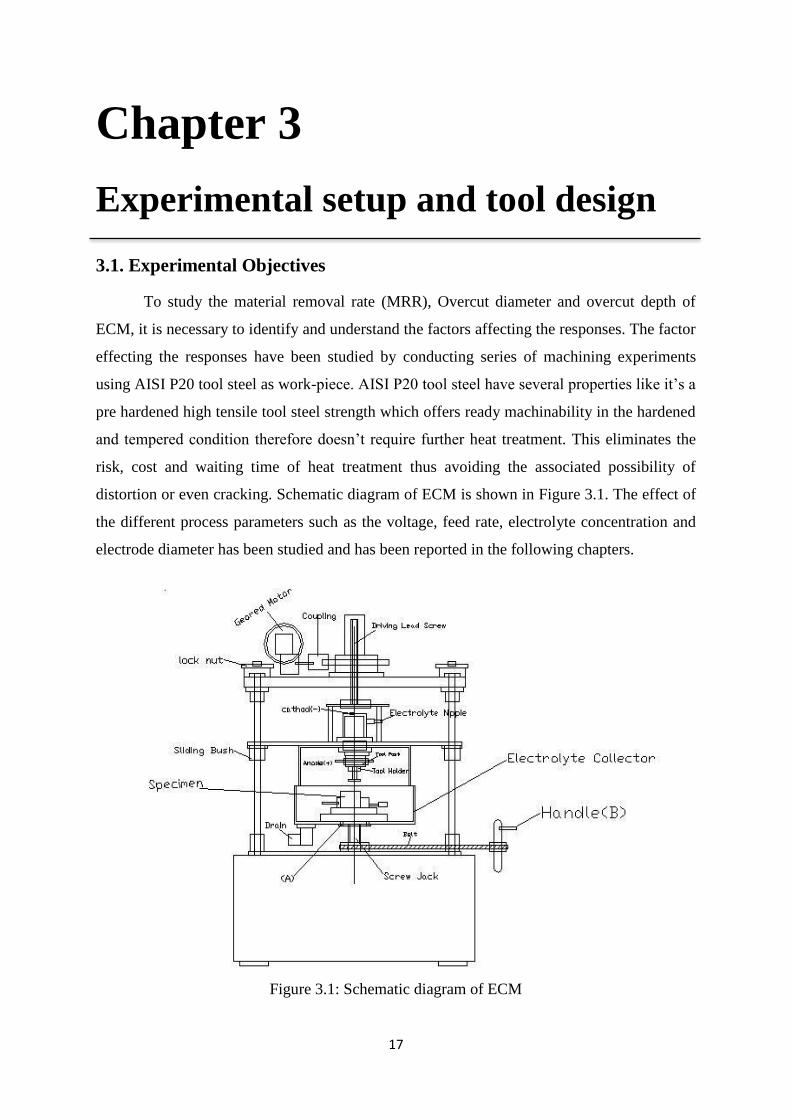
3.1. Experimental Objectives
To study the material removal rate (MRR), Overcut diameter and overcut depth of
ECM, it is necessary to identify and understand the factors affecting the responses. The factor
effecting the responses have been studied by conducting series of machining experiments
using AISI P20 tool steel as work-piece. AISI P20 tool steel have several properties like it’s a
pre hardened high tensile tool steel strength which offers ready machinability in the hardened
and tempered condition therefore doesn’t require further heat treatment. This eliminates the
risk, cost and waiting time of heat treatment thus avoiding the associated possibility of
distortion or even cracking. Schematic diagram of ECM is shown in Figure 3.1. The effect of
the different process parameters such as the voltage, feed rate, electrolyte concentration and
electrode diameter has been studied and has been reported in the following chapters.
Figure 3.1: Schematic diagram of ECM
18
3.2. Experimental Setup
The whole experimental conducted on Electrochemical Machining set up from
Metatech Industry, Pune which is having input Supply of - 415 v +/- 10%, 3 phase AC, 50
HZ. Output supply is 0-300A DC at any voltage from 0-25V and efficiency is better than
80% at partial and full load condition. The cable insulation resistance is not less than 10
Mega ohms with 500V DC. And consist of three major sub systems which are being
discussed in this chapter. The set up consists of three major sub systems.
1. Machining setup
2. Control Panel
3. Electrolyte Circulation
3.2.1. Machining Setup
This electro-mechanical assembly is a sturdy structure, associated with precision machined
components, servo motorized vertical up/down movement of tool, an electrolyte dispensing
arrangement, illuminated machining chamber with see through window, job fixing vice, job
table lifting mechanism and sturdy stand. All the exposed components, parts have undergone
proper material selection and coating/plating for corrosion protection. ECM setup is shown in
Figure 3.2.
Figure 3.2: ECM Setup
19
Technical Data
Tool area - 30 mm2.
Cross head stroke - 150 mm.
Job holder - 100 mm opening X 50 mm depth X 100 mm width.
Tool feed motor - DC Servo type.
3.2.2. Control Panel
Through control panel we adjust the current (I), voltage (V), feed rate (F) and time (T) for
duration of experiment. The power supply is a perfect integration of, high current electrical,
power electronics and precision programmable microcontroller based technologies. Since the
machine operates at very low voltage, there are no chances of any electrical shocks during
operation. Control Panel shown in Figure 3.3.
Figure 3.3: Control Panel

20
Technical Data
Electrical Out Put Rating – 0 - 300 Amps. DC at any voltage from 0 - 20 V.
Efficiency - Better than 80% at partial & full load condition.
Protections - Over load, Short circuit, single phasing.
Operation Modes - Manual/Automatic.
Timer - 0 - 99.9 min.
Tool Feed - 0.2 to 2 mm/min.
Z Axis Control - Forward, reverse, auto forward /reverse, through micro controller.
Supply - 415 v +/- 10%, 3 - phase AC, 50 Hz.
3.2.3. Electrolyte Circulation
The electrolyte is pumped from a tank, lined by corrosion resistant coating with the
help of corrosion resistant pump firstly it fed to filter then it’s fed to the job. Spent
electrolyte will return to the tank. The hydroxide sludge arising will settle at the bottom of
the tank & can be easily drained out. Electrolyte supply shall be governed by flow control
valve. Extra electrolyte flow is by passed to the tank. Reservoir provides separate settling
and siphoning compartments. All fittings are of corrosion resistant material or of Stainless
steel, as necessary.
Figure 3.4 Electrolyte tank with Filter
3.3. Tool Setup:
The purpose of the experimental investigation was to find out the Material removal
rate, Overcut diameter and Overcut depth of plane work pieces made of AISI P20 tool steel.
21
The tools were made up of copper. It is an abridged general view of the experimental system.
The experimental conditions are: the electrolyte is sodium chloride, the electrode gap
between the tool and work piece is 0.1 to 0.3 mm, the work piece is 100 mm diameter and 50
mm thickness and the cathode is copper. When the experiment is carried out, the electrolyte
should be at room temperature each time and after the experiment the conductivity of
electrolyte must be checked. And while doing the experiment some overcuts are occurred so
that overcut diameter and depth is taken with the help of Coordinate Measurement Machine
(CMM).
After reviewing number of papers there is still some work that has to be done in the area
of electrochemical machining with rotary tool. So in this experimental work the circular
cavity is formed on the work piece by using Rotary U-shaped tubular copper electrode. So to
rotate the U-shaped copper electrode, three devices are necessary as follows.
1. Gear Box.
2. Variable dc controller and
3. Rotary U- Shaped Tool electrode.
3.3.1. Gear Box
Gearboxes provide speed and torque conversion between two rotating shafts for a
given gear ratio and it is a major part of this experimental setup. This gear box consists of
pinion gear, face gear, double spur gear and spur gear as shown in Figure 3.5. A maximum
gear ratio of 1:4 has to be maintained for speed reduction at every stage. Two gear boxes with
gear ratio 1:60 were assembled in series to obtain an output speed of 0.25 rpm from a driven
DC motor at 600 to 800 rpm. The speed of the motor was controlled with variable DC
controller ranging from 0.5 to 3v. Figure 3.6 show the assembly of reduction gear box.
Table 3.1: Gear specifications used in the gearbox
Gear no Name Gear teeth (driver /driven)
1. Pinion 10 Teeth (T)/ -
2. Face 14 T / 36 T
3. Double spur 14 T / 36 T
4. Double spur 14 T / 36 T
5. Spur 10 T / 36 T
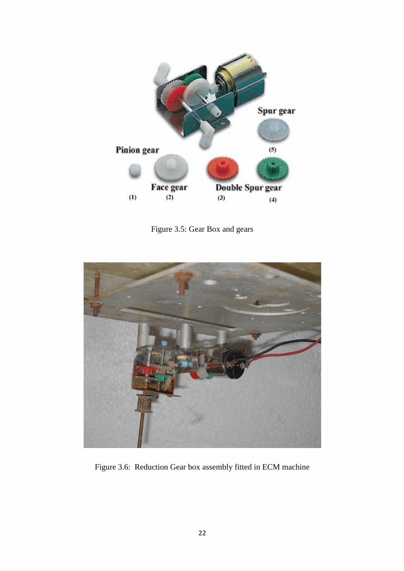
22
Figure 3.5: Gear Box and gears
Figure 3.6: Reduction Gear box assembly fitted in ECM machine
23
3.3.2. Variable DC Power Controller
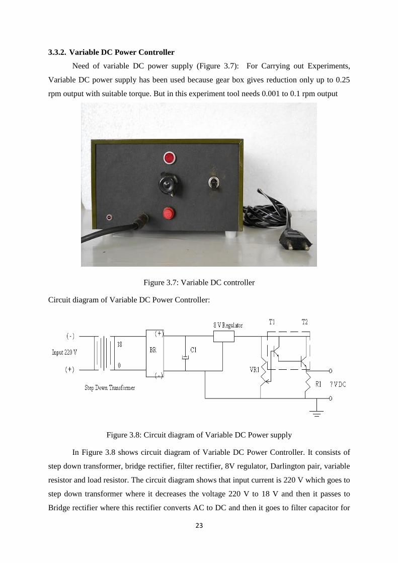
Need of variable DC power supply (Figure 3.7): For Carrying out Experiments,
Variable DC power supply has been used because gear box gives reduction only up to 0.25
rpm output with suitable torque. But in this experiment tool needs 0.001 to 0.1 rpm output
Figure 3.7: Variable DC controller
Circuit diagram of Variable DC Power Controller:
Figure 3.8: Circuit diagram of Variable DC Power supply
In Figure 3.8 shows circuit diagram of Variable DC Power Controller. It consists of
step down transformer, bridge rectifier, filter rectifier, 8V regulator, Darlington pair, variable
resistor and load resistor. The circuit diagram shows that input current is 220 V which goes to
step down transformer where it decreases the voltage 220 V to 18 V and then it passes to
Bridge rectifier where this rectifier converts AC to DC and then it goes to filter capacitor for
24
filtering. Filter capacitors are common in electrical and electronic work, and cover a number
of applications. It filters low pass, high pass, notch, etc. and mostly used for smooth DC
power supplies. After then it goes to 8V regulator where it regulates the voltage and from
there it goes for Darlington Pair. A Darlington pair is used to amplify weak signals so that
they can be clearly detected by another circuit. The two transistors are known as a Darlington
pair. Without a Darlington pair the circuit would probably fail. And from Darlington pair it
goes to variable resistor (10 turn). A variable resistor controls the amount of current flowing
through part of a circuit. The amount of current can be changed by changing the setting of the
resistor. The knob on a Variable DC Power Controller is a variable resistor. When the knob is
turned one direction the resistance increases. This decreases or increases the current flowing
and the speed can be controlled according to the requirement. After that it goes to load
resistor and the output from load resistor will be given as input for the motor.
3.3.3. Rotary U-Shaped tool electrode
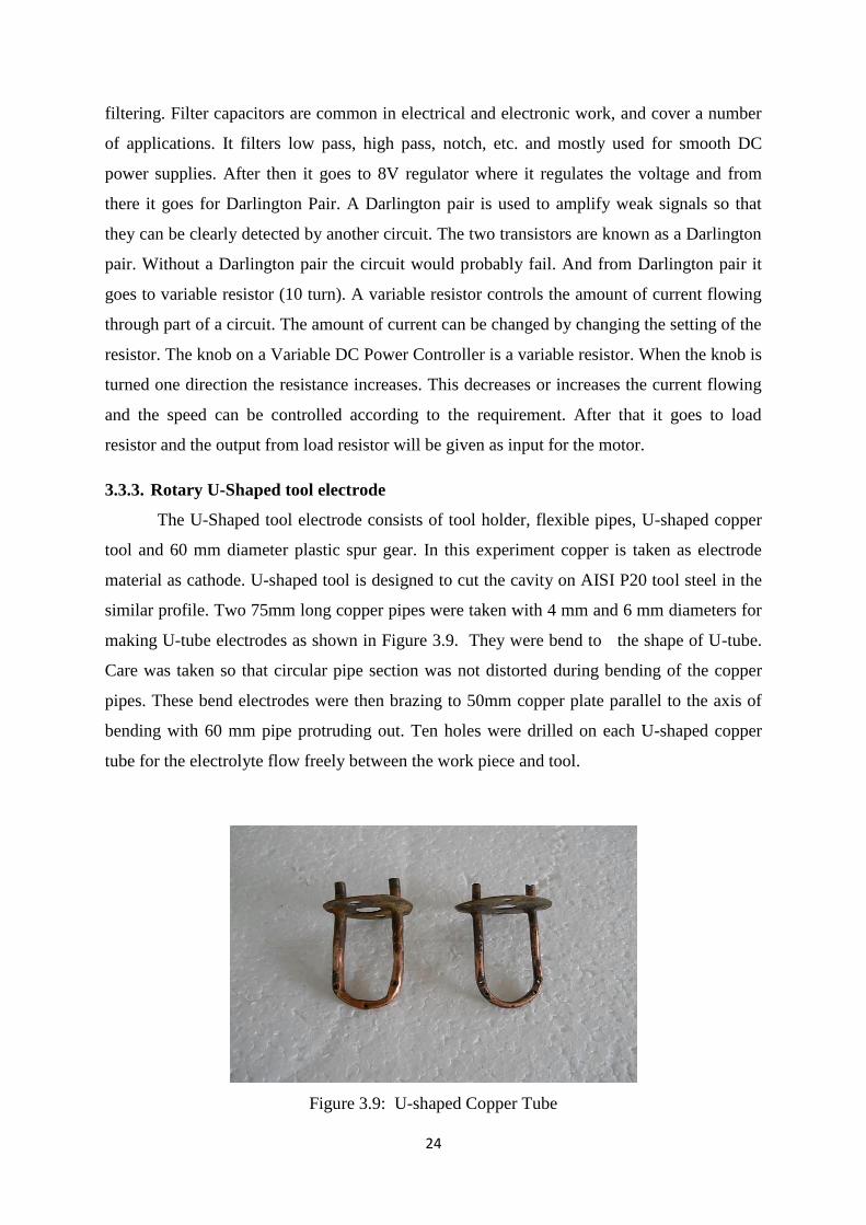
The U-Shaped tool electrode consists of tool holder, flexible pipes, U-shaped copper
tool and 60 mm diameter plastic spur gear. In this experiment copper is taken as electrode
material as cathode. U-shaped tool is designed to cut the cavity on AISI P20 tool steel in the
similar profile. Two 75mm long copper pipes were taken with 4 mm and 6 mm diameters for
making U-tube electrodes as shown in Figure 3.9. They were bend to the shape of U-tube.
Care was taken so that circular pipe section was not distorted during bending of the copper
pipes. These bend electrodes were then brazing to 50mm copper plate parallel to the axis of
bending with 60 mm pipe protruding out. Ten holes were drilled on each U-shaped copper
tube for the electrolyte flow freely between the work piece and tool.
Figure 3.9: U-shaped Copper Tube
25
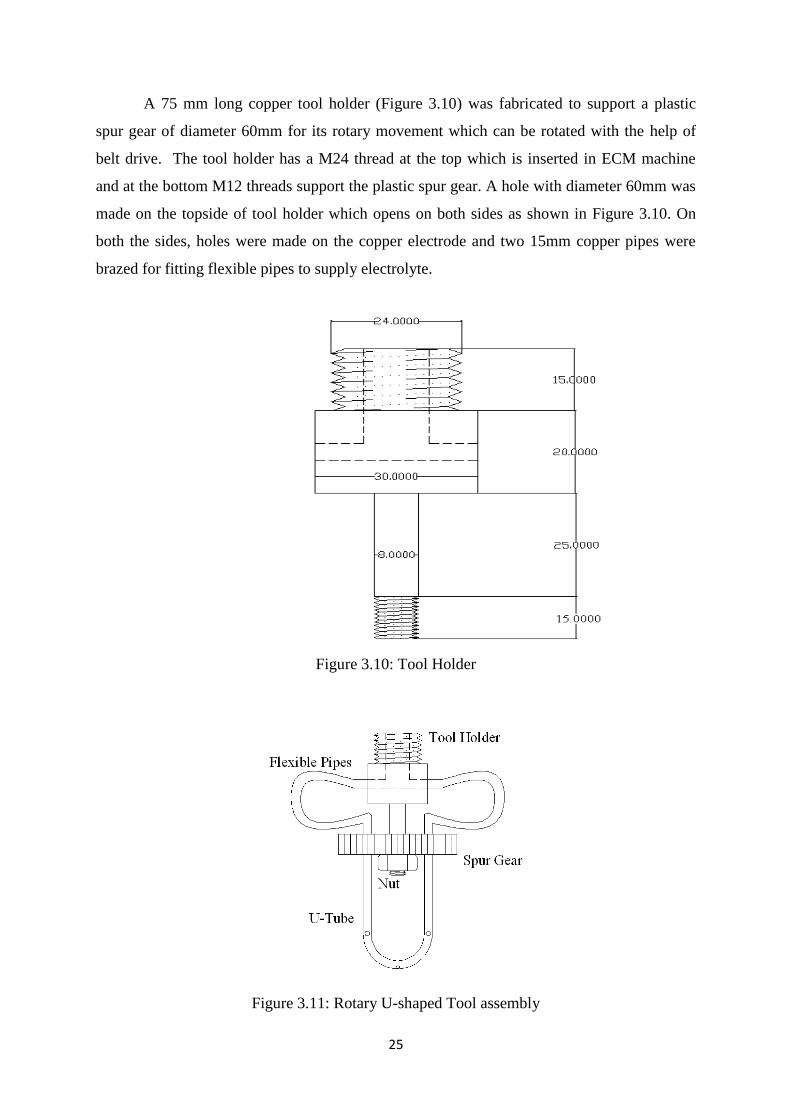
A 75 mm long copper tool holder (Figure 3.10) was fabricated to support a plastic
spur gear of diameter 60mm for its rotary movement which can be rotated with the help of
belt drive. The tool holder has a M24 thread at the top which is inserted in ECM machine
and at the bottom M12 threads support the plastic spur gear. A hole with diameter 60mm was
made on the topside of tool holder which opens on both sides as shown in Figure 3.10. On
both the sides, holes were made on the copper electrode and two 15mm copper pipes were
brazed for fitting flexible pipes to supply electrolyte.
Figure 3.10: Tool Holder
Figure 3.11: Rotary U-shaped Tool assembly
26
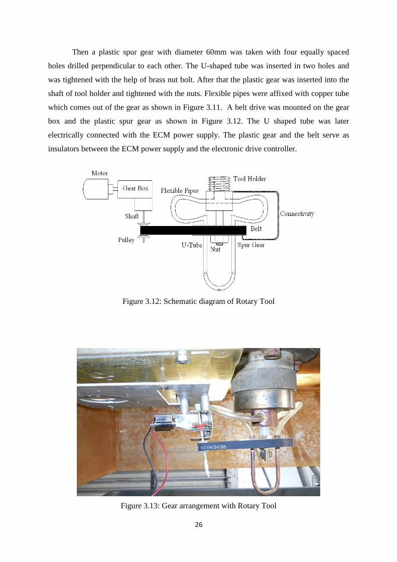
Then a plastic spur gear with diameter 60mm was taken with four equally spaced
holes drilled perpendicular to each other. The U-shaped tube was inserted in two holes and
was tightened with the help of brass nut bolt. After that the plastic gear was inserted into the
shaft of tool holder and tightened with the nuts. Flexible pipes were affixed with copper tube
which comes out of the gear as shown in Figure 3.11. A belt drive was mounted on the gear
box and the plastic spur gear as shown in Figure 3.12. The U shaped tube was later
electrically connected with the ECM power supply. The plastic gear and the belt serve as
insulators between the ECM power supply and the electronic drive controller.
Figure 3.12: Schematic diagram of Rotary Tool
Figure 3.13: Gear arrangement with Rotary Tool

27
3.4 Conclusion:
A U shaped tool was designed for this experiment along with gear reduction and variable DC
controller for suitable rotary feed for the experiment.
28
Chapter 4 Experimental Work
In this chapter experimental work is discussed which is based on Taguchi orthogonal
array L16. MRR, overcut diameter and depth of the work piece were measured and Grey
relational analysis is adopted to find the best parameters setting.
4.1. Specification of Work-piece material:
Experiment was conducted on AISI P20 tool steel as a work-piece. The specification
of the material is given in Table 4.1 and chemical composition in Table 4.2. The mechanical
and thermal properties are presented in Table 4.3. Work-piece dimension was 100 mm in
diameter and 60 mm thickness. Five such pieces of AISI P20 steel were taken to conduct 16
experimental runs.
Table 4.1: Description of AISI P20 steel
Category Steel
Class Tool Steel
Type General mold steel
Designations Germany: DIN 1.2330
United States: ASTM A681, FED QQ-T-570, UNS T51620
Table 4.2: Work piece Composition
Element C Mn Si Cr Mo Cu P S
Weight % 0.28-0.40 0.60-1.00 0.20-0.80 1.40-2.00 0.30-0.55 0.25 0.03 0.03
Table 4.3: Mechanical and Thermal Properties
Parameter Temperature(T °
C)
Density (×1000 kg/m3) at 25 ° C 7.85 25
Poisson's Ratio 0.270-0.30 25
Elastic Modulus (GPa) 190-210 25
Thermal Expansion (10-6
/ºC) 12.8 20-425(more)

29
4.2. Taguchi Experimental Design and Analysis
4.2.1. Taguchi’s Philosophy
Taguchi’s comprehensive system of quality engineering is one of the engineering
achievements of the 20th
century. His methods focus on the effective application of
engineering strategies rather than advanced statistical techniques. It includes both upstream
and shop-floor quality engineering. Upstream methods efficiently use small-scale
experiments to reduce variability and remain cost-effective and robust design for large-scale
production and market place. Shop-floor techniques provide cost-based, real time methods
for monitoring and maintaining quality in production. The farther upstream a quality method
is applied, the greater leverages it produces on the improvement, and the more it reduces the
cost and time. Taguchi’s philosophy is founded on the following three very simple and
fundamental concepts:
Quality should be designed into the product and not inspected into it.
Quality is best achieved by minimizing the deviations from the target. The product
or process should be so designed that it is immune to uncontrollable environmental
variables.
The cost of quality should be measured as a function of deviation from the standard
and the losses should be measured system-wide.
Taguchi proposes an “off-line” strategy for quality improvement as an alternative to an
attempt to inspect quality into a product on the production line. He observes that poor quality
cannot be improved by the process of inspection, screening and salvaging. No amount of
inspection can put quality back into the product. Taguchi recommends a three-stage process:
system design, parameter design and tolerance design. In the present work Taguchi’s design
approach is used to study the effect of process parameter on the various responses of the
ECM process.
4.2.2. Experimental Design Strategy
Taguchi’s recommends orthogonal array (OA) for laying out of experiments. These
OA’s are generalised Graeco-Latin squares. To design an experiment is to select the most
suitable OA and to assign the parameters and interaction of interest to the appropriate
columns. The use of linear graphs and triangular table suggested by Taguchi makes the
assignment of parameters simple. The array forces all experimenters to design almost
identical experiments.
30
In the Taguchi method the results of the experiments are analysed to achieve one or
more of the following objectives:
To establish the best or the optimum condition for a product or process
To estimate the contribution of individual parameters and interactions
To estimate the response under the optimum condition
The optimum condition is identified by studying the main effect of each of the
parameters. The main effects indicate the general trends of influence of each parameter. The
analysis of variance (ANOVA) is the statistical treatment most commonly applied to the
results of the experiments in determining the per cent contribution of each parameter against
a stated level of confidence. Study of ANOVA table for a given analysis helps to determine
which of the parameters need control.
In the present investigation the analysis of variance (ANOVA) has been performed.
The effect of the selected ECM process parameters on the selected responses have been
investigated through the plots of the main effects based on ANOVA. The optimum condition
for each of the quality characteristics has been estimated through analysis of variance.
In the experiment, Minitab 14 software for Taguchi design was used. In this study, 2
level design (four factors) with total of 16 numbers of experiments to be conducted and hence
the OA L16 was chosen. The machining parameters and their level are shown in Table 4.4.
Table 4.4 Machining parameters and there levels
Machining Parameter Symbol Unit Level
Level 1 Level 2
Voltage V v 10 15
Feed Rate F mm/min 0.3 0.6
Electrolyte concentration C g/l 30 50
Electrode Diameter D mm 4 6
Flow rate - lpm 10
4.3. Making of Brine Solution:
In the ECM process the making of brine solution plays an important role in
material removal rate. Brine solution was prepared by adding common salt with
31
water by maintaining the conductivity of the water. In this experiment we have taken
two different concentration of electrolyte i.e. 30 g/l and 50 g/l it means mixture 30 gram of
salt in 1 liter of normal water and 50 gram of salt in 1 liter of normal water respectively.
4.4. Experimental Procedure:
This experiment is mainly conducted in two steps.
Step 1: The initial weight of the work piece has to be taken for calculation of MRR. Keeping
the flow rate constant at 10 l/m and the rest of the parameters are set according to
Table 4.5 for each run. Work piece was kept in horizontal position, and by using the
U-shaped electrode machining was started from the position “C” shown in Figure
4.1. Care has to be taken such that tip of the electrode should not touch the surface
of the work-piece. The U-shaped electrode was fed up to the depth of 25mm inside
the work piece. During the whole process the machining time was noted down. In
this step only vertical feed motion has been taken rotation of tool has done on next
step.
Figure 4.1: Machining step 1
Step 2:
In this step, the vertical feed of the tool was stopped and it was fed in circular
direction at constant rpm. After tool rotated a half revolution, the cavity was formed
Feed
32
on the work-piece. The final stage after step 2 is shown In Figure 4.2. The final
weight of the work-piece was noted and the machining time was being noted down.
Figure 4.2: After Machining in step 2
Figure 4.3: Work-piece after machining (number inscribed represents run order)
Figure 4.3 shows the work-piece of after machining first four runs after machining. Figure
4.4 shows the work-piece of AISI P20 tool steel material after machining Run order number
5th
, 6th
, 7th
and 8th
. Figure 4.5 shows the work-piece of AISI P20 tool steel material after
machining Run order number 9th
, 10th
, 11th
and 12th
. Figure 4.6 shows the work-piece of
33
AISI P20 tool steel material after machining Run order number 13th
, 14th
, 15th
and 16th
. The
experimental observations are tabulated in Table 4.5.
Figure 4.4: Work-piece after machining 5th
, 6th
, 7th
and 8th
run
Figure 4.5: Work-piece after machining 9th
, 10th
, 11th
and 12th
run
34
Figure 4.6: Work-piece after machining 13th
, 14th
, 15th
and 16th
run
Table 4.5: Experimental observations using L16 orthogonal array
Run
order
Voltage
(V)
Feed (F)
mm/min
Electrolyte
concentration
(C) g/l
Tool
Diameter
(D) mm
MRR
(mm3/min)
OC
diameter
(mm)
OC
Depth
(mm)
1 10 0.3 30 4 0.05600 4.825 6.500
2 10 0.3 30 6 0.04431 4.929 6.730
3 10 0.3 50 4 0.05830 4.812 6.287
4 10 0.3 50 6 0.05550 4.856 6.609
5 10 0.6 30 4 0.09850 5.128 6.980
6 10 0.6 30 6 0.09870 5.260 7.180
7 10 0.6 50 4 0.10800 5.089 6.830
8 10 0.6 50 6 0.09890 5.212 7.080
9 15 0.3 30 4 0.09120 4.893 6.620
10 15 0.3 30 6 0.07970 4.972 6.880
11 15 0.3 50 4 0.09110 4.853 6.474
12 15 0.3 50 6 0.08880 4.966 6.830
13 15 0.6 30 4 0.13510 5.207 7.274
14 15 0.6 30 6 0.12800 5.301 7.410
15 15 0.6 50 4 0.13640 5.208 7.140
16 15 0.6 50 6 0.12750 5.256 7.376

35
4.6. Sample Calculations (For run order 1):
MRR is calculated as given by the following formula:
RR initial weight final weight
density total time
Overcut-diameter is calculated as given by the following formula:
OC observed diameter actual diameter
2 observed diameter 35
2
Overcut- depth is calculated as given by the following formula:
Overcut depth over depth – actual depth over depth – 25
4.7. Grey relation analysis
In the grey relation analysis, experiment data, i.e., measured responses, are first
normalised in the range of 0 to 1. This process is called grey relation generation. Based on
this data, grey relation coefficients are calculated to represent the correlation between the
ideal (best) and the actual normalized experimental data. Overall, grey relation grade is then
determined by averaging the grey relation coefficient corresponding to selected responses.
The overall quality characteristics of the multi-response process depend on the calculated
grey relation grade.
4.7.1. Grey relation generation
There are three different types of data normalization according to the requirement of
Lower the Better (LB), Higher the Better (HB), or Nominal the Best (NB) criteria. The
desired quality characteristics for MRR are HB criterion; therefore, the normalization of
original sequence of these three responses is done using equation (1).
yi*(k)
yi(k) min yi(k)
max yi(k) min yi(k) ( )
36
Where yi*(k) is the normalised data, i.e. after grey relational generation, yi(k) is the k
th
response of the ith
experiment, min yi(k) is the smallest value of yi(k) for kth
response, and
max yi(k) is the largest value of yi(k) for the kth
response.
Overcut diameter and overcut depth follows the LB criterion. Accordingly, the
normalization of these responses is done using equation (2).
yi*(k)
max yi(k) yi(k)
max yi(k) min yi(k) ( )
4.7.2. Grey relation coefficient
The grey relation coefficient is calculated as
i(k) min max
oi(k) max ( )
Where (k) is the grey relation coefficient of the ith
experiment for the kth
response,
( )=||y*0(k)-y
*i(k)||, i.e. , absolute of the difference between y
*0(k) and y
*i(k), y
*0(k) is the
ideal or reference sequence, = maxi maxk||y*
0(k)-y*i(k)|| is the largest value of , and
mini maxk||y*0(k)-y
*i(k)|| is the smallest value of , and (0≤ ≤1) is the
distinguish coefficient.
4.7.3. Grey relation grade
The grey relation grade (Ґi) is calculated by averaging the grey relational coefficients
corresponding to each experiment.
1
n
1
Qi(k) ( )
Where, Q is the total number of response and n is the number of output responses. The
grey relational grade Ґi represents the level of correlation between the reference sequence and
the comparability sequence. If higher grey relation grade occurred than the corresponding
parameter combination is closer to the optimal setting.
Sample calculation for Grey relation:
For run order 1
Normalised value of MRR Y1(MRR) = ( )
( ) = 0.1269
Normalised value of OC-dep Y1(OC-dep) =( )
( ) = 0.8103
Grey relation coefficient of MRR 1(MRR) =
( ) = 0.3642
37
Grey relation coefficient of OC-dep 1(OC-dep) =
( ) = 0.7250
Grey relation grade of run order 1 is Ґ1 =
= 0.5446
Table 4.6 Evaluated grey relational grade for responses
Now calculate the grey relation grade for 16 number of experiment and those values have
maximum in the specific run order which has closes the optimal condition. In this experiment
the OC-diameter and OC-depth are co-related so, here OC-depth and MRR has been consider
as responses. In Grey relational analysis of the experimental result of material removal rate
and overcut depth can be simplified into the optimization of a single response that is Grey
relational grade (GRG). This methodology for optimising the process parameters of ECM of
P20 tool steel considering 4 input parameters and 2 output parameters. Two output responses
MRR, OC-depth and there GRG for each experiment using L16 OA based on Taguchi design
is shown in Table 4.6. And experimental number verse GRG plot are shown in Figure 4.7.
This Figure indicates process parameter setting of Run 15 has highest grey relational grade.
Run order Normalized values Grey relational analysis Grey relational coefficient Grade
MRR OC-dep MRR OC-dep MRR OC-dep
1 0.1269 0.8103 0.8731 0.1897 0.3642 0.7250 0.5446
2 0.0000 0.6055 1.0000 0.3945 0.3333 0.5590 0.4462
3 0.1519 1.0000 0.8481 0.0000 0.3709 1.0000 0.6854
4 0.1215 0.7133 0.8785 0.2867 0.3627 0.6355 0.4991
5 0.5884 0.3606 0.4116 0.6394 0.5485 0.4388 0.4937
6 0.5906 0.2048 0.4094 0.7952 0.5498 0.3860 0.4679
7 0.6916 0.5165 0.3084 0.4835 0.6185 0.5084 0.5634
8 0.5928 0.2939 0.4072 0.7061 0.5511 0.4145 0.4828
9 0.5092 0.7035 0.4908 0.2965 0.5046 0.6277 0.5662
10 0.3843 0.4720 0.6157 0.5280 0.4481 0.4864 0.4673
11 0.5081 0.8335 0.4919 0.1665 0.5041 0.7502 0.6271
12 0.4831 0.5165 0.5169 0.4835 0.4917 0.5084 0.5000
13 0.9859 0.1211 0.0141 0.8789 0.9725 0.3626 0.6676
14 0.9088 0.0000 0.0912 1.000 0.8457 0.3333 0.5895
15 1.000 0.2404 0.0000 0.7596 1.0000 0.3970 0.6985
16 0.9034 0.0303 0.0966 0.9697 0.8380 0.3402 0.5891
38
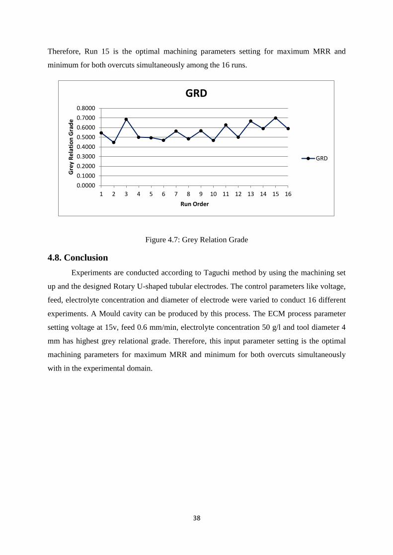
Therefore, Run 15 is the optimal machining parameters setting for maximum MRR and
minimum for both overcuts simultaneously among the 16 runs.
Figure 4.7: Grey Relation Grade
4.8. Conclusion
Experiments are conducted according to Taguchi method by using the machining set
up and the designed Rotary U-shaped tubular electrodes. The control parameters like voltage,
feed, electrolyte concentration and diameter of electrode were varied to conduct 16 different
experiments. A Mould cavity can be produced by this process. The ECM process parameter
setting voltage at 15v, feed 0.6 mm/min, electrolyte concentration 50 g/l and tool diameter 4
mm has highest grey relational grade. Therefore, this input parameter setting is the optimal
machining parameters for maximum MRR and minimum for both overcuts simultaneously
with in the experimental domain.
0.0000
0.1000
0.2000
0.3000
0.4000
0.5000
0.6000
0.7000
0.8000
1 2 3 4 5 6 7 8 9 10 11 12 13 14 15 16
Gre
y R
ela
tio
n G
rad
e
Run Order
GRD
GRD

39
Chapter 5
Result and Discussion
In this chapter the effect of process parameter on responses such as MRR, Overcut
diameter and Overcut depth are analysed.
5.1. Analysis of Experiment and Discussions:
5.1.1. Effect on MRR
The machinability of ECM depends on the electrical conductivity of the electrolyte,
feed rate of electrode, inter electrode gap and electrolyte flow rate. The influence of various
machining parameters on MRR (means) are shown in Fig. 5.1. The electrode feed rate has
enormous effect on MRR and it increases with increase in feed rate. This result was expected
because the material removal rate increases with feed rate because the machining time
decreases. MRR also increases with voltage and electrolyte concentration; however, the
effect is less than the feed rate on MRR, while by increasing the tool diameter MRR
decreases and the effect of tool diameter and concentration of electrolyte has very little effect
on RR and doesn’t give any conclusive evidence of any impact on RR.
Figure 5.1: Main effect Plot for MRR

40
In Table 5.1, ANOVA of MRR is presented with all the terms. The columns in table
represent source of variation (source), degree of freedom (DF), sequential sum of squares
(Seq. SS), adjusted sum of squares (Adj. SS), adjusted mean sum of squares (Adj. MS), F-
value (F), and p-value. The significant factors are Voltage, Feed and diameter of tube,
whereas all interactions factors are found to be insignificant. After eliminating non-
significant sources i.e. interaction of process parameter like V*F, V*D, V*D, F*C, F*D, C*D
terms, the results are shown in Table 5.2.
Table 5.1: ANOVA for MRR
Source
DF Seq. SS Adj. SS Adj. MS F P
Volt (V) 1 0.004212 0.004212 0.004212 322.46 0.000
Feed (F) 1 0.008381 0.008381 0.008381 641.68 0.000
Electrolyte
Concentration(C)
1 0.000068 0.000068 0.000068 5.21 0.071
Diameter (D) 1 0.000177 0.000177 0.000177 13.54 0.014
V*F 1 0.000012 0.000012 0.000012 0.91 0.384
V*C 1 0.000011 0.000011 0.000011 0.86 0.397
V*D 1 0.000003 0.000003 0.000003 0.20 0.676
F*C 1 0.000009 0.000009 0.000009 0.69 0.445
F*D 1 0.000001 0.000001 0.000001 0.05 0.824
C*D 1 0.000003 0.000003 0.000003 0.23 0.649
Error 5 0.000065 0.000065 0.000013
Total 15 0.012941
Table 5.2: ANOVA for MRR after eliminating non-significant values
Source DF Seq. SS Adj. SS Adj. MS F P
Volt (V) 1 0.004212 0.004212 0.004212 446.66 0.000
Feed (F) 1 0.008381 0.008381 0.008381 888.83 0.000
Electrolyte
Concentration (C)
1 0.000068 0.000068 0.000068 7.21 0.021
Diameter (D) 1 0.000177 0.000177 0.000177 18.75 0.001
Error 11 0.000104 0.000104 0.000009
Total 15 0.012941
41
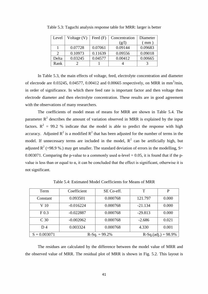
Table 5.3: Taguchi analysis response table for MRR: larger is better
In Table 5.3, the main effects of voltage, feed, electrolyte concentration and diameter
of electrode are 0.03245, 0.04577, 0.00412 and 0.00665 respectively, on MRR in mm3/min,
in order of significance. In which there feed rate is important factor and then voltage then
electrode diameter and then electrolyte concentration. These results are in good agreement
with the observations of many researchers.
The coefficients of model mean of means for MRR are shown in Table 5.4. The
parameter R2 describes the amount of variation observed in MRR is explained by the input
factors. R2 = 99.2 % indicate that the model is able to predict the response with high
accuracy. Adjusted R2 is a modified R
2 that has been adjusted for the number of terms in the
model. If unnecessary terms are included in the model, R2 can be artificially high, but
adjusted R2 (=98.9 %.) may get smaller. The standard deviation of errors in the modelling, S=
0.003071. Comparing the p-value to a commonly used α-level = 0.05, it is found that if the p-
value is less than or equal to α, it can be concluded that the effect is significant, otherwise it is
not significant.
Table 5.4: Estimated Model Coefficients for Means of MRR
Term Coefficient SE Co-eff. T P
Constant 0.093501 0.000768 121.797 0.000
V 10 -0.016224 0.000768 -21.134 0.000
F 0.3 -0.022887 0.000768 -29.813 0.000
C 30 -0.002062 0.000768 -2.686 0.021
D 4 0.003324 0.000768 4.330 0.001
S = 0.003071 R-Sq. = 99.2% R-Sq.(adj.) = 98.9%
The residues are calculated by the difference between the model value of MRR and
the observed value of MRR. The residual plot of MRR is shown in Fig. 5.2. This layout is
Level Voltage (V) Feed (F) Concentration
(g/l)
Diameter
( mm )
1 0.07728 0.07061 0.09144 0.09683
2 0.10973 0.11639 0.09556 0.09018
Delta 0.03245 0.04577 0.00412 0.00665
Rank 2 1 4 3
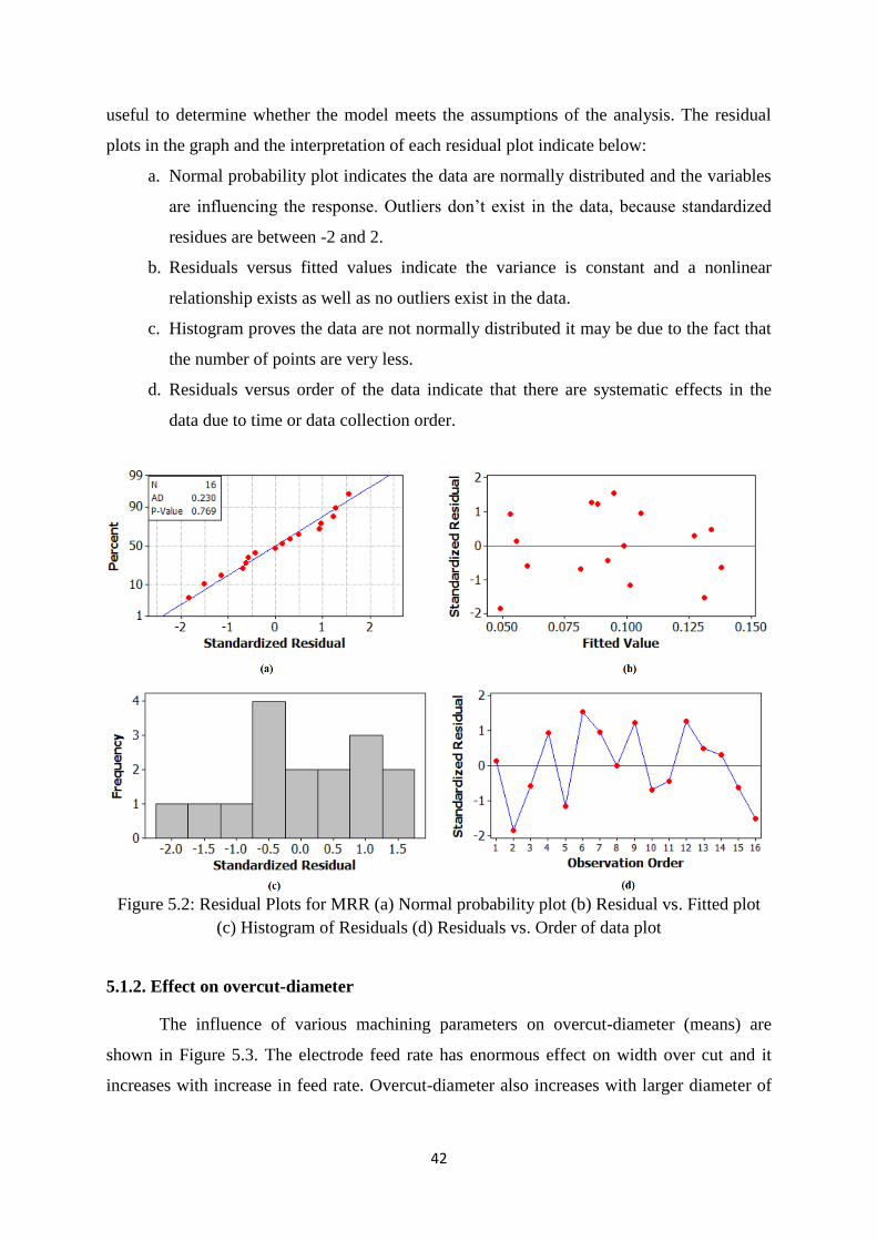
42
useful to determine whether the model meets the assumptions of the analysis. The residual
plots in the graph and the interpretation of each residual plot indicate below:
a. Normal probability plot indicates the data are normally distributed and the variables
are influencing the response. Outliers don’t exist in the data, because standardized
residues are between -2 and 2.
b. Residuals versus fitted values indicate the variance is constant and a nonlinear
relationship exists as well as no outliers exist in the data.
c. Histogram proves the data are not normally distributed it may be due to the fact that
the number of points are very less.
d. Residuals versus order of the data indicate that there are systematic effects in the
data due to time or data collection order.
Figure 5.2: Residual Plots for MRR (a) Normal probability plot (b) Residual vs. Fitted plot
(c) Histogram of Residuals (d) Residuals vs. Order of data plot
5.1.2. Effect on overcut-diameter
The influence of various machining parameters on overcut-diameter (means) are
shown in Figure 5.3. The electrode feed rate has enormous effect on width over cut and it
increases with increase in feed rate. Overcut-diameter also increases with larger diameter of
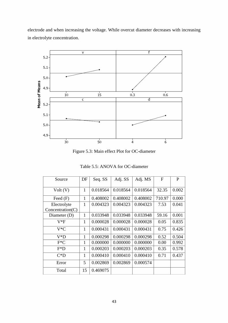
43
electrode and when increasing the voltage. While overcut diameter decreases with increasing
in electrolyte concentration.
Figure 5.3: Main effect Plot for OC-diameter
Table 5.5: ANOVA for OC-diameter
Source
DF Seq. SS Adj. SS Adj. MS F P
Volt (V) 1 0.018564 0.018564 0.018564 32.35 0.002
Feed (F) 1 0.408002 0.408002 0.408002 710.97 0.000
Electrolyte
Concentration(C)
1 0.004323 0.004323 0.004323 7.53 0.041
Diameter (D) 1 0.033948 0.033948 0.033948 59.16 0.001
V*F 1 0.000028 0.000028 0.000028 0.05 0.835
V*C 1 0.000431 0.000431 0.000431 0.75 0.426
V*D 1 0.000298 0.000298 0.000298 0.52 0.504
F*C 1 0.000000 0.000000 0.000000 0.00 0.992
F*D 1 0.000203 0.000203 0.000203 0.35 0.578
C*D 1 0.000410 0.000410 0.000410 0.71 0.437
Error 5 0.002869 0.002869 0.000574
Total 15 0.469075
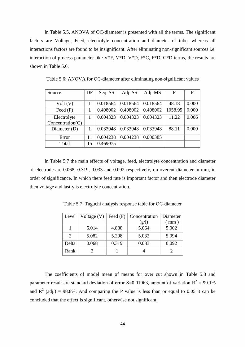
44
In Table 5.5, ANOVA of OC-diameter is presented with all the terms. The significant
factors are Voltage, Feed, electrolyte concentration and diameter of tube, whereas all
interactions factors are found to be insignificant. After eliminating non-significant sources i.e.
interaction of process parameter like V*F, V*D, V*D, F*C, F*D, C*D terms, the results are
shown in Table 5.6.
Table 5.6: ANOVA for OC-diameter after eliminating non-significant values
In Table 5.7 the main effects of voltage, feed, electrolyte concentration and diameter
of electrode are 0.068, 0.319, 0.033 and 0.092 respectively, on overcut-diameter in mm, in
order of significance. In which there feed rate is important factor and then electrode diameter
then voltage and lastly is electrolyte concentration.
Table 5.7: Taguchi analysis response table for OC-diameter
The coefficients of model mean of means for over cut shown in Table 5.8 and
parameter result are standard deviation of error S=0.01963, amount of variation R2 = 99.1%
and R2 (adj.) = 98.8%. And comparing the P value is less than or equal to 0.05 it can be
concluded that the effect is significant, otherwise not significant.
Source DF Seq. SS Adj. SS Adj. MS F P
Volt (V) 1 0.018564 0.018564 0.018564 48.18 0.000
Feed (F) 1 0.408002 0.408002 0.408002 1058.95 0.000
Electrolyte
Concentration(C)
1 0.004323 0.004323 0.004323 11.22 0.006
Diameter (D) 1 0.033948 0.033948 0.033948 88.11 0.000
Error 11 0.004238 0.004238 0.000385
Total 15 0.469075
Level Voltage (V) Feed (F) Concentration
(g/l)
Diameter
( mm )
1 5.014 4.888 5.064 5.002
2 5.082 5.208 5.032 5.094
Delta 0.068 0.319 0.033 0.092
Rank 3 1 4 2
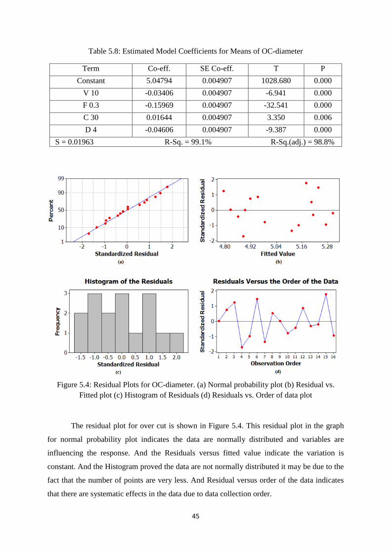
45
Table 5.8: Estimated Model Coefficients for Means of OC-diameter
Term Co-eff. SE Co-eff. T P
Constant 5.04794 0.004907 1028.680 0.000
V 10 -0.03406 0.004907 -6.941 0.000
F 0.3 -0.15969 0.004907 -32.541 0.000
C 30 0.01644 0.004907 3.350 0.006
D 4 -0.04606 0.004907 -9.387 0.000
S = 0.01963 R-Sq. = 99.1% R-Sq.(adj.) = 98.8%
Figure 5.4: Residual Plots for OC-diameter. (a) Normal probability plot (b) Residual vs.
Fitted plot (c) Histogram of Residuals (d) Residuals vs. Order of data plot
The residual plot for over cut is shown in Figure 5.4. This residual plot in the graph
for normal probability plot indicates the data are normally distributed and variables are
influencing the response. And the Residuals versus fitted value indicate the variation is
constant. And the Histogram proved the data are not normally distributed it may be due to the
fact that the number of points are very less. And Residual versus order of the data indicates
that there are systematic effects in the data due to data collection order.
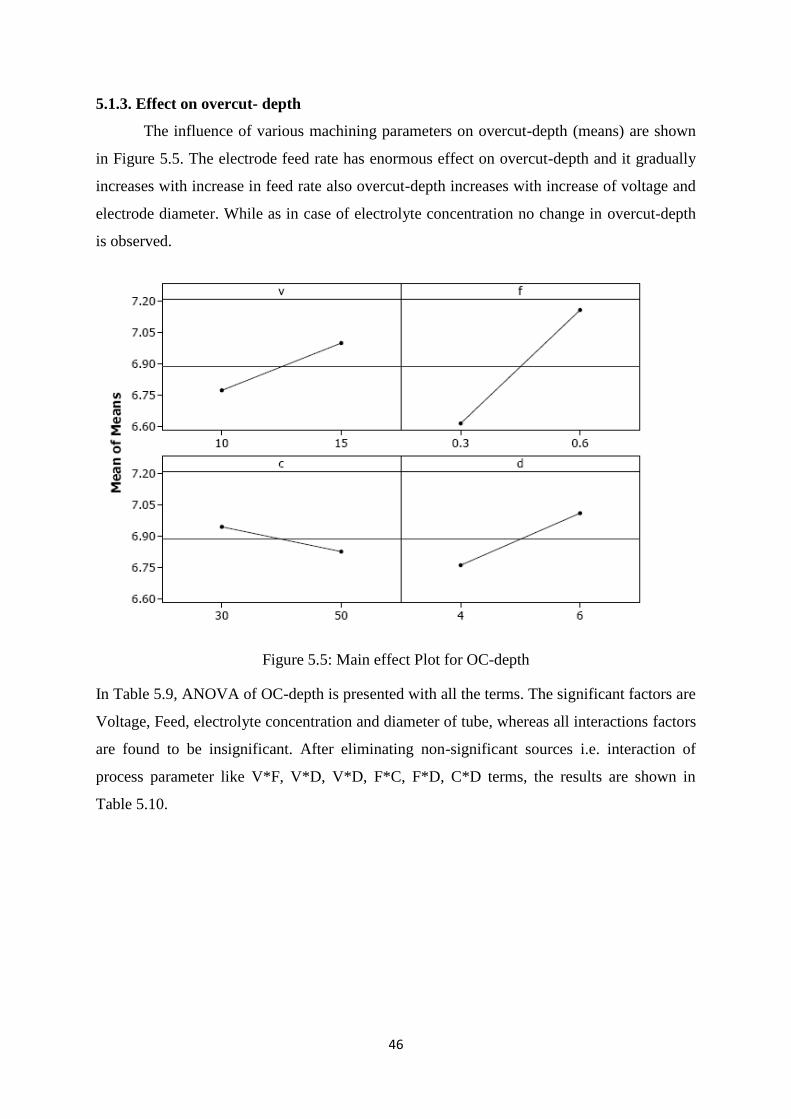
46
5.1.3. Effect on overcut- depth
The influence of various machining parameters on overcut-depth (means) are shown
in Figure 5.5. The electrode feed rate has enormous effect on overcut-depth and it gradually
increases with increase in feed rate also overcut-depth increases with increase of voltage and
electrode diameter. While as in case of electrolyte concentration no change in overcut-depth
is observed.
Figure 5.5: Main effect Plot for OC-depth
In Table 5.9, ANOVA of OC-depth is presented with all the terms. The significant factors are
Voltage, Feed, electrolyte concentration and diameter of tube, whereas all interactions factors
are found to be insignificant. After eliminating non-significant sources i.e. interaction of
process parameter like V*F, V*D, V*D, F*C, F*D, C*D terms, the results are shown in
Table 5.10.
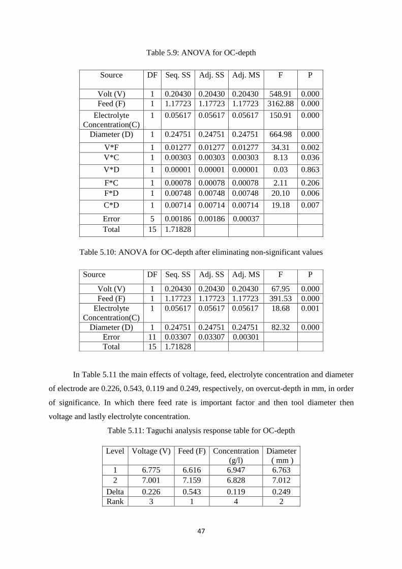
47
Table 5.9: ANOVA for OC-depth
Table 5.10: ANOVA for OC-depth after eliminating non-significant values
In Table 5.11 the main effects of voltage, feed, electrolyte concentration and diameter
of electrode are 0.226, 0.543, 0.119 and 0.249, respectively, on overcut-depth in mm, in order
of significance. In which there feed rate is important factor and then tool diameter then
voltage and lastly electrolyte concentration.
Table 5.11: Taguchi analysis response table for OC-depth
Source
DF Seq. SS Adj. SS Adj. MS F P
Volt (V) 1 0.20430 0.20430 0.20430 548.91 0.000
Feed (F) 1 1.17723 1.17723 1.17723 3162.88 0.000
Electrolyte
Concentration(C)
1 0.05617 0.05617 0.05617 150.91 0.000
Diameter (D) 1 0.24751 0.24751 0.24751 664.98 0.000
V*F 1 0.01277 0.01277 0.01277 34.31 0.002
V*C 1 0.00303 0.00303 0.00303 8.13 0.036
V*D 1 0.00001 0.00001 0.00001 0.03 0.863
F*C 1 0.00078 0.00078 0.00078 2.11 0.206
F*D 1 0.00748 0.00748 0.00748 20.10 0.006
C*D 1 0.00714 0.00714 0.00714 19.18 0.007
Error 5 0.00186 0.00186 0.00037
Total 15 1.71828
Source DF Seq. SS Adj. SS Adj. MS F P
Volt (V) 1 0.20430 0.20430 0.20430 67.95 0.000
Feed (F) 1 1.17723 1.17723 1.17723 391.53 0.000
Electrolyte
Concentration(C)
1 0.05617 0.05617 0.05617 18.68 0.001
Diameter (D) 1 0.24751 0.24751 0.24751 82.32 0.000
Error 11 0.03307 0.03307 0.00301
Total 15 1.71828
Level Voltage (V) Feed (F) Concentration
(g/l)
Diameter
( mm )
1 6.775 6.616 6.947 6.763
2 7.001 7.159 6.828 7.012
Delta 0.226 0.543 0.119 0.249
Rank 3 1 4 2

48
Table 5.12: Estimated Model Coefficients for Means of OC-depth
Term Co-eff. SE Co-eff. T P
Constant 6.88750 0.01371 502.431 0.000
V 10 -0.11300 0.01371 -8.243 0.000
F 0.3 -0.27125 0.01371 -19.787 0.000
C 30 0.05925 0.01371 4.322 0.001
D 4 -0.12438 0.01371 -9.073 0.000
S = 0.05483 R-Sq. = 98.1% R-Sq.(adj.) = 97.4%
The coefficients of model mean of means for over cut depth is shown in Table 5.12
and parameter result are standard deviation of error S=0.05483, amount of variation R2 =
98.1% and R2 (adj.) = 97.4%. And comparing the P value is less than or equal to 0.05 it can
be concluded that the effect is significant, otherwise not significant.
Figure 5.6: Residual Plots for OC-depth. (a) Normal probability plot (b) Residual vs. Fitted
plot (c) Histogram of Residuals (d) Residuals vs. Order of data plot
The residual plot for over cut is shown in Figure 5.6. This residual plot in the graph
for normal probability plot indicates the data are normally distributed and variables are
influencing the response. And the Residuals versus fitted value indicate the variation is
constant. And the Histogram proved the data are not normally distributed it may be due to the

49
fact that the number of points are very less. And Residual versus order of the data indicates
that there are systematic effects in the data due to data collection order.
5.2. Conclusion:
The work evaluates the feasibility of machining blind cavity on AISI P20 tool steel in ECM
with Rotary U-shaped electrode. Among the four process parameters, feed rate influences
highly the responses followed by voltage and then electrode diameter. Electrolyte
concentration has very little effect on Response.
50
Chapter 6
Conclusion
In the present study, four factors are considered voltage, feed rate, electrolyte concentration
and tool diameter. AISI P20 steel as a work-piece and 16 experiments to be conducted to
obtain an optimum level in achieving high material removal rate, minimize OC-diameter and
minimize OC-depth. The following conclusions are arrived:
Among the four process parameters, feed rate influences highly the MRR, followed
by applied voltage then electrode diameter and then by the concentration of
electrolyte.
For both OC-diameter and OC-depth the most influencing parameter are feed rate
followed by electrode diameter then voltage and lastly the concentration of
electrolyte.
From the grey relation grade, the optimal machining parameter setting are obtained
for Run 15 i.e. voltage = 15 V, feed = 0.6 mm/min, electrolyte concentration = 50 g/l
and electrode diameter = 4 mm for maximizing MRR and minimizing overcut
diameter and depth.
51
References
[1] J.A. McGeough, Principle of Electrochemical Machining, Chapman and Hall, London,
1974.
[2] H. El-hofy, Fundamentals of Machining Processes, Conventional and Nonconventional
Processes, Taylor & Francis Group, 2007.
[3] D. Zhu, K. Wang, J.M. Yang, Design of Electrode Profile in Electrochemical
Manufacturing Process, CIRP Annals-Manufacturing Technology 52 (1) 169-172.
[4] YUMING ZHOU and JEFFREY J. DERBY, The Cathode Design Problem in
Electrochemical Machining, Chemical Engineering Science, 50(17) (1995) 2679- 2689.
[5] C.S. CHANG, L.W. HOURNG, C.T. CHUNG, Tool design in electrochemical machining
considering the effect of thermal-fluid properties, Journal of Applied Electrochemistry,
29 (1999) 321-330.
[6] S.J. Ebeid, M.S. Hewidy, T.A. El-Taweel, A.H. Youssef, Towards higher accuracy for
ECM hybridized with low-frequency vibrations using the response surface methodology,
Journal of Materials Processing Technology 149 (2004) 432-438.
[7] P.S.Pa, Effective form design of electrode in electrochemical smoothing of end turning
surface finishing, Journal of materials processing technology 195 (2008) 44-52.
[8] Chunhua Sun, Di Zhu, Zhiyong Li, Lei Wang, Application of FEM to tool design for
electrochemical machining freeform surface, Finite Elements in Analysis and Design 43
(2006) 168-172.
[9] J.A. Westley, J. Atkinson, A. Duffield, Generic aspects of tool design for electrochemical
machining, Journal of Materials Processing Technology 149 (2004) 384-392.
[10] M.S. Amalnik, J.A. McGeough, Intelligent Concurrent Manufacturability Evaluation of
Design for Electrochemical Machining, Journal of Materials Processing Technology 61
(1996) 130-139.
[11] K.P. Rajurkar and M.S. Hewidy, Effect of Grain Size on ECM Performance, Journal of
Mechanical Working Technology, 17 (1988) 315 - 324.
[12] K.P. Rajurkar, D. Zhu, B. Wei, Minimization of Machining Allowance in
Electrochemical Machining, Annals of the CIRP Vol. 47(1998) 165-168.
52
[13] M.S. Hewidy, Controlling of metal removal thickness in ECM process, Journal of
Materials Processing Technology 160 (2005) 348-353.
[14] I. Strode and M. B. Bassett, The effect of Electrochemical Machining on the Surface
Integrity and Mechanical Properties of Cast AND Wrought Steels, Wear, 109 (1966)
171- 180.
[15] Ming-Chang Jeng, Ji-Liang Doong and Chih-Wen Yang, The effects of carbon content
and microstructure on the metal removal rate in Electrochemical Machining, Journal of
Materials Processing Technology, 38 (1993) 527-538.
[16] S.C. TAM, N.H. LOH, Optimization of the ECM-Abrasive Polishing of Mild Steel Using
Response Surface Methodology, Journal of Mechanical Working Technology, 19 (1989)
109-117.
[17] J.J. Sun, E.J. Taylor, R. Srinivasan, MREF-ECM process for hard passive materials
surface finishing, Journal of Materials Processing Technology 108 (2001) 356-368.
[18] Shuo-Jen Lee, Yu-Ming Lee, Ming-Feng Du, The polishing mechanism of
electrochemical mechanical polishing technology, Journal of Materials Processing
Technology 140 (2003) 280–286.
[19] H. Hocheng, P.S. Pa, The application of a turning tool as the electrode in
electropolishing, Journal of Materials Processing Technology 120 (2002) 6-12.
[20] Baocheng Wang and Jinhua Zhu, Effect of electrochemical polishing time on surface
topography of mild steel, Journal of University of Science and Technology 14 (2007)
236-239.
[21] A.K.M. De Silva , H.S.J. Altena, JA. McGeough, Influence of Electrolyte Concentration
on Copying Accuracy of Precision-ECM, Annals of the CIRP, 49.
[22] Petr Novak, Ivo Rousar, Rudolf Stefec, Vladmir Cihal, Intergranular corrosion in
Electrochemical Machining, Materials Chemistry and Physics 10 (1984) 155-161.
[23] M.A. Bejar and F. Gutierrez, On the determination of current efficiency in
electrochemical machining with a variable gap, Journal of Materials Processing
Technology, 37 (1993) 691-699.
[24] M.A. Bejar, F. Eterovich, Wire-electrochemical cutting with a NaNO3 electrolyte,
Journal of Materials Processing Technology 55 (1995) 417- 420.
[25] T. Haisch, E. Mittemeijer, J.W. Schultze, Electrochemical machining of the steel 100Cr6
in aqueous NaCl and solutions: microstructure of surface films formed by
carbides, Electrochimica Acta 47 (2001) 235–241.
53
[26] D. Zhu, W. Wang, X.L. Fang, N.S. Qu, Z.Y. Xu, Electrochemical drilling of multiple
holes with electrolyte-extraction, CIRP Annals - Manufacturing Technology 59 (2010)
239–242.
[27] Xiangyu Zhao, Liqun Ma, Meng Yang, Yi Ding, Xiaodong Shen, Electrochemical
properties of Ti–Ni–H powders prepared by milling titanium hydride and nickel,
international journal of hydrogen energy xxx (2009) 1-4.
[28] Minghuan Wang,Wei Peng ,Chunyan Yao, Electrochemical machining of the spiral
internal turbulator, International Journal of Advanced Manufacturing Technology 49
(2010) 969–973.
54
Dissemination of Work
Published
1. Rahul Ganjir, C.K.Biswas and Shailesh Dewangan,, “Estimation of RR on
Electrochemical achining by using Taguchi ethod”, International Conference on
Innovative Science & Engineering Technology, (ICISET-2011), pp 362-365, 8-9 April,
2011, Rajkot, India.
Top Related