Download - MLS Sample

8/3/2019 MLS Sample

http://slidepdf.com/reader/full/mls-sample 1/10

Economic and Market Watch Report

3rd Quarter, 2002

*Click on a County to view economic and real estate information at the county and zip code level

© 2002 Trend MLS and NATIONAL ASSOCIATION OF REALTORS®

Reproduction, reprinting, or retransmission in any form is prohibited without written

permission.

8/3/2019 MLS Sample


Trend MLS Economic and Market Watch Report

TRe N D is one of the ten largest regional Multiple Listing Service’s (MLS) in the country, delivering

MLS data services to over 18,000 real estate professionals throughout a thirteen county network.

TRe N D is committed to providing real estate professionals with superior real estate marketinformation services and making technology accessible through education, communication, and

support. The TRe N D family of e-products and services: MLSWeb™, REALIST.com, The

GoTRe N D! Private Network, WyldFyre Listings™, and www.trendmls.com provides the

knowledge, technology, and service REALTORS® need to succeed in today’s competitive real

estate marketplace.

TRe N D is pleased to introduce the Economic and Market Watch Report designed to help real

estate practitioners identify current and future economic and real estate trends that affect our

industry.

Local Report…………………………….....……………………….………..2

Pennsylvania

Berks County…………………………………………………………2

Bucks County…………………………………………………………3

Chester County……………………………………………………….4

Delaware County……………………………………………………..5

Montgomery County…………………………………………………6

Philadelphia County……………………………………………….…7

New Jersey

Burlington County……………………………………………..…….8

Camden County………………………………………………..…….9Gloucester County………………………………………………..….10

Mercer County…………………………………………………...…..11

Salem County………………………………………..……………….12

Delaware

Kent County…………………………………………………….……13

New Castle County……………………………………………….….14

Trends……………………………………………………….....………….....15

Chief Economist’s Commentary………………………………….....…...…17

Local Forecast………………………………………………….....……...….19

Economic Monitor…………………………………………….....……….....21

Index

1

8/3/2019 MLS Sample


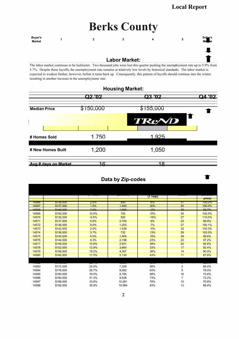
Berks County

Local Report

2

Buyer's

Market1 2 3 4 5

Seller's

Market

Labor Market:The labor market continues to be lackluster. Two thousand jobs were lost this quarter pushing the unemployment rate up to 5.9% from

5.7%. Despite these layoffs, the unemployment rate remains at relatively low levels by historical standards. The labor market is

expected to weaken further, however, before it turns back up. Consequently, this pattern of layoffs should continue into the winter

resulting in another increase in the unemployment rate.

Housing Market:

Q2 '02 Q3 '02 Q4 '02

Median Price $150,000 $155,000

# Homes on the Market

16 18

Data by Zip-codes

Zip Code Median PricePrice Change

(1 Year)

Total # Homes Sold

(Quarter)

% change in #

homes sold

(1 Year)

Average Days on

Market

% of asking

price

(sold/list

price)

14566 $135,000 2.0% 500 6% 31 100.0%

14567 $137,000 1.0% 1,400 30% 20 105.0%

14568 $146,000 7.0% 1,900 -2% 35 99.7%

14569 $150,200 10.0% 750 10% 30 102.0%

14570 $135,200 -0.5% 920 -16% 27 110.0%

14571 $137,500 5.0% 2,700 9% 23 99.9%

14572 $136,000 9.0% 1,203 7% 27 100.1%

14573 $142,500 2.0% 1,539 -5% 32 100.3%

14574 $136,500 3.7% 732 13% 29 102.0%

14575 $140,500 6.0% 1,465 18% 26 99.6%

14576 $144,500 8.3% 2,198 23% 23 97.2%

14577 $148,500 10.6% 2,931 28% 20 94.8%

14578 $152,500 12.9% 3,664 33% 17 92.4%

14579 $156,500 15.2% 4,397 38% 14 90.0%

14580 $160,500 17.5% 5,130 43% 11 87.6%

14581 $164,500 19.8% 5,863 48% 8 85.2%

14582 $168,500 22.1% 6,596 53% 5 82.8%

14583 $172,500 24.4% 7,329 58% 2 80.4%

14584 $176,500 26.7% 8,062 63% 5 78.0%

14585 $180,500 29.0% 8,795 68% 16 75.6%

14586 $184,500 31.3% 9,528 73% 7 73.2%

14587 $188,500 33.6% 10,261 78% 10 70.8%

14588 $192,500 35.9% 10,994 83% 13 68.4%

Avg # days on Market

1,200

4,100 3,910

# New Homes Built 1,050

1,750 1,925 # Homes Sold

8/3/2019 MLS Sample


15

Trends

Full Price?

90%

92%

94%

96%

98%

100%

102%

7 days or

less

8 to 14

days

15 to 30

days

31 to 60

days

61 to 90

days

more than

90 days

Days on Market

P

e r c e n t o f S a l e s P r i c e

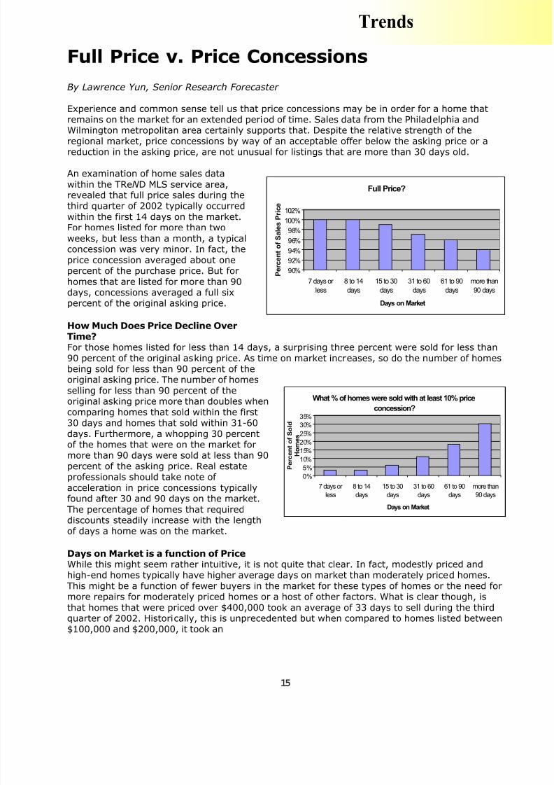
Full Price v. Price Concessions

By Lawrence Yun, Senior Research Forecaster

Experience and common sense tell us that price concessions may be in order for a home thatremains on the market for an extended period of time. Sales data from the Philadelphia andWilmington metropolitan area certainly supports that. Despite the relative strength of the

regional market, price concessions by way of an acceptable offer below the asking price or areduction in the asking price, are not unusual for listings that are more than 30 days old.

An examination of home sales datawithin the TReN D MLS service area,revealed that full price sales during thethird quarter of 2002 typically occurredwithin the first 14 days on the market.For homes listed for more than twoweeks, but less than a month, a typicalconcession was very minor. In fact, theprice concession averaged about one

percent of the purchase price. But forhomes that are listed for more than 90days, concessions averaged a full sixpercent of the original asking price.

How Much Does Price Decline OverTime?For those homes listed for less than 14 days, a surprising three percent were sold for less than90 percent of the original asking price. As time on market increases, so do the number of homesbeing sold for less than 90 percent of theoriginal asking price. The number of homesselling for less than 90 percent of theoriginal asking price more than doubles when

comparing homes that sold within the first30 days and homes that sold within 31-60days. Furthermore, a whopping 30 percentof the homes that were on the market formore than 90 days were sold at less than 90percent of the asking price. Real estateprofessionals should take note of acceleration in price concessions typicallyfound after 30 and 90 days on the market.The percentage of homes that requireddiscounts steadily increase with the lengthof days a home was on the market.

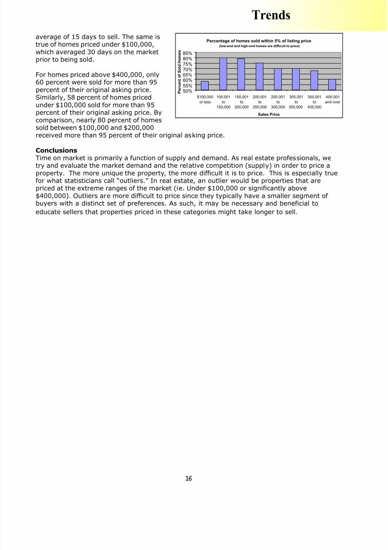
Days on Market is a function of PriceWhile this might seem rather intuitive, it is not quite that clear. In fact, modestly priced andhigh-end homes typically have higher average days on market than moderately priced homes.This might be a function of fewer buyers in the market for these types of homes or the need formore repairs for moderately priced homes or a host of other factors. What is clear though, isthat homes that were priced over $400,000 took an average of 33 days to sell during the thirdquarter of 2002. Historically, this is unprecedented but when compared to homes listed between$100,000 and $200,000, it took an

What % of homes were sold with at least 10% price

concession?

0%

5%

10%

15%

20%

25%

30%

35%

7 days or

less

8 to 14

days

15 to 30

days

31 to 60

days

61 to 90

days

more than

90 days

Days on Market

P e r c e n t o f S o l d

H o m e s

8/3/2019 MLS Sample


average of 15 days to sell. The same istrue of homes priced under $100,000,which averaged 30 days on the marketprior to being sold.

For homes priced above $400,000, only60 percent were sold for more than 95percent of their original asking price.

Similarly, 58 percent of homes pricedunder $100,000 sold for more than 95percent of their original asking price. Bycomparison, nearly 80 percent of homessold between $100,000 and $200,000received more than 95 percent of their original asking price.

ConclusionsTime on market is primarily a function of supply and demand. As real estate professionals, wetry and evaluate the market demand and the relative competition (supply) in order to price aproperty. The more unique the property, the more difficult it is to price. This is especially truefor what statisticians call “outliers.” In real estate, an outlier would be properties that arepriced at the extreme ranges of the market (ie. Under $100,000 or significantly above$400,000). Outliers are more difficult to price since they typically have a smaller segment of buyers with a distinct set of preferences. As such, it may be necessary and beneficial to

educate sellers that properties priced in these categories might take longer to sell.

Percentage of homes sold within 5% of listing price(low-end and high-end homes are difficult to price)

50%55%60%65%70%75%80%85%

$100,000or less

100,001to

150,000

150,001to

200,000

200,001to

250,000

250,001to

300,000

300,001to

350,000

350,001to

400,000

400,001and over

Sales Price

P e r c e n t o f S o l d H o m e s

Trends

16

8/3/2019 MLS Sample


Chief Economist’s Comment

17

A Bird’s Eye View

By David Lereah, Chief Economist

If you were able to take flight, soar 10,000 feet above the earth and look down at the U.S.economy – you could be surprised at what you saw. What you would see is an economy that is

fundamentally sound with favorable prospects. Consumers are spending money on goods andservices. Business inventories are relatively lean. Borrowing costs – those headline- makinginterest rates – are near historic lows. Both the housing and automobile markets are flourishing.Foreign capital is flowing freely. Unemployment is well below six percent, and inflation isrelatively tame. Putting all this together, one would conclude that the view from 10,000 feet of this low inflation/low interest rate environment presents a favorable backdrop for a robustrecovery.

So what’s wrong with this picture? Why is the economy struggling to lift itself up from therecession of 2001? Upon closer inspection other items come into view. Let’s take a look at someof them.

· The U.S. equities market continues to be in retreat; company stock values have dropped

collectively by more than $7 trillion since March 2000.

· The industrial sector is displaying unusual weakness at this stage of the recovery.

· The manufacturing sector is contracting once again, as measured by a 49.5 ISM Indexfor September (below 50 reflects contraction).

· Consumer confidence, as measured by the Conference Board Consumer Confidence Indexhas fallen for the fourth consecutive month (September).

· The labor markets continue to display unusual sluggishness in a recovery, averaging only40,000 payroll gains per month since May.

All of these factors help explain why the economy continues along its sluggish path, but they donot tell the full story.

The Bounce TheoryHistorically, recovery periods usually have a strong “bounce back” effect from recessions. Since1970 there have been four recovery periods (excluding the present one). GDP growth during thefirst year in each of those recovery periods was well above 3 percent – actually, averaging 4.6percent growth for the four recoveries taken as a whole. But according to most projections,including our own NAR forecast (see page 6), the 2002 recovery will experience about 2.5percent GDP growth, significantly lower than previous recoveries.

So why is there no “bounce back” effect in today’s economy? While the economy appears to befundamentally and structurally sound, there doesn’t seem to be much vigor in economic activity– there’s no “oomph.” There are some intangible factors that might help explain today’slackluster performance.

First, the economy continues to absorb the residual effects from the bursting of the technologybubble. After climbing to higher and higher heights of both investment and profitabilitythroughout the 1990s, the technology sector finally hit the ceiling and crashed. The magnitudeof the fall more than equaled its ascent, and it has generated a significant amount of disruptionfor many sectors of the economy.

8/3/2019 MLS Sample


Similarly, the economy continues to be negatively influenced from the fallout of the equitiesmarket. The positive wealth effect of the 1990s stock market has now turned negative and isexerting downward pressure on consumer spending. The stock market decline has cut householdwealth (from peak to trough) by $7 trillion from March 2000. Based on the Federal Reserve’sestimates of the stock market’s wealth effect, this translates into about a $280 billion reductionin consumer spending. That, in turn, slows economic activity.

And finally, there is that intangible factor that currently casts a dark shadow across the U.S.

economy – negative psychology. The combination of a plunging stock market, corporatescandals and the fight against terrorism and potential war with Iraq weighs very heavily onpeople’s minds, generating uncertainty and shattering confidence – both impediments to aneconomic recovery.

But there are still some good views from 10,000 feet. Housing is one. In spite of the war onterror, stock market slides, and falling consumer confidence, people are still out there buyinghomes. With interest rates at historically low levels and demand for homeownership unwavering,existing home sales are poised to set a record in 2002. There may be some things that don’tlook so nice when we’re flying so high, but other scenes – like people buying homes andbecoming homeowners – are beautiful to behold.

Chief Economist’s Commenta

18

Real Estate Outlook

8/3/2019 MLS Sample


The Forecast

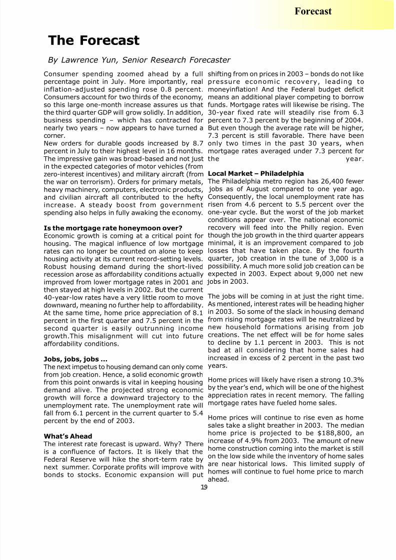
By Lawrence Yun, Senior Research Forecaster

19

Forecast

Consumer spending zoomed ahead by a fullpercentage point in July. More importantly, realinflation-adjusted spending rose 0.8 percent.

Consumers account for two thirds of the economy,so this large one-month increase assures us thatthe third quarter GDP will grow solidly. In addition,business spending – which has contracted fornearly two years – now appears to have turned acorner.New orders for durable goods increased by 8.7percent in July to their highest level in 16 months.The impressive gain was broad-based and not justin the expected categories of motor vehicles (fromzero-interest incentives) and military aircraft (fromthe war on terrorism). Orders for primary metals,heavy machinery, computers, electronic products,

and civilian aircraft all contributed to the heftyincrease. A steady boost from governmentspending also helps in fully awaking the economy.

Is the mortgage rate honeymoon over?Economic growth is coming at a critical point forhousing. The magical influence of low mortgagerates can no longer be counted on alone to keephousing activity at its current record-setting levels.Robust housing demand during the short-livedrecession arose as affordability conditions actuallyimproved from lower mortgage rates in 2001 andthen stayed at high levels in 2002. But the current40-year-low rates have a very little room to movedownward, meaning no further help to affordability.At the same time, home price appreciation of 8.1percent in the first quarter and 7.5 percent in thesecond quarter is easily outrunning incomegrowth.This misalignment will cut into futureaffordability conditions.

Jobs, jobs, jobs ...The next impetus to housing demand can only comefrom job creation. Hence, a solid economic growthfrom this point onwards is vital in keeping housing

demand alive. The projected strong economicgrowth will force a downward trajectory to theunemployment rate. The unemployment rate willfall from 6.1 percent in the current quarter to 5.4percent by the end of 2003.

What’s AheadThe interest rate forecast is upward. Why? Thereis a confluence of factors. It is likely that theFederal Reserve will hike the short-term rate bynext summer. Corporate profits will improve withbonds to stocks. Economic expansion will put

shifting from on prices in 2003 – bonds do not likepressure economic recovery, leading tomoneyinflation! And the Federal budget deficit

means an additional player competing to borrowfunds. Mortgage rates will likewise be rising. The30-year fixed rate will steadily rise from 6.3percent to 7.3 percent by the beginning of 2004.But even though the average rate will be higher,7.3 percent is still favorable. There have beenonly two times in the past 30 years, whenmortgage rates averaged under 7.3 percent forthe year.

Local Market – PhiladelphiaThe Philadelphia metro region has 26,400 fewer

jobs as of August compared to one year ago.

Consequently, the local unemployment rate hasrisen from 4.6 percent to 5.5 percent over theone-year cycle. But the worst of the job marketconditions appear over. The national economicrecovery will feed into the Philly region. Eventhough the job growth in the third quarter appearsminimal, it is an improvement compared to joblosses that have taken place. By the fourthquarter, job creation in the tune of 3,000 is apossibility. A much more solid job creation can beexpected in 2003. Expect about 9,000 net new

jobs in 2003.

The jobs will be coming in at just the right time.As mentioned, interest rates will be heading higherin 2003. So some of the slack in housing demandfrom rising mortgage rates will be neutralized bynew household formations arising from jobcreations. The net effect will be for home salesto decline by 1.1 percent in 2003. This is notbad at all considering that home sales hadincreased in excess of 2 percent in the past twoyears.

Home prices will likely have risen a strong 10.3%by the year’s end, which will be one of the highest

appreciation rates in recent memory. The fallingmortgage rates have fueled home sales.

Home prices will continue to rise even as homesales take a slight breather in 2003. The medianhome price is projected to be $188,800, anincrease of 4.9% from 2003. The amount of newhome construction coming into the market is stillon the low side while the inventory of home salesare near historical lows. This limited supply of homes will continue to fuel home price to marchahead.

8/3/2019 MLS Sample


20

Forecast

2002

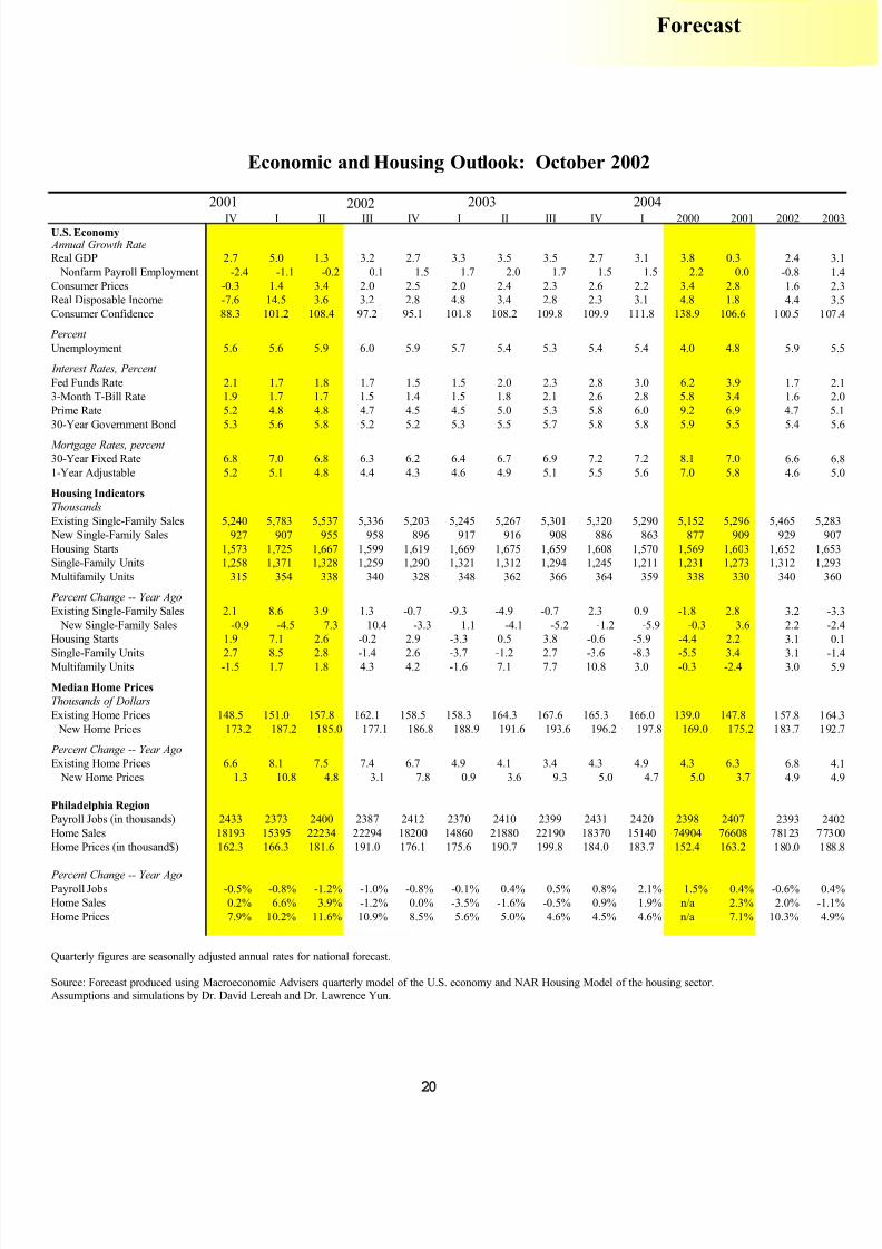
IV I II III IV I II III IV I 2000 2001 2002 2U.S. Economy

Annual Growth RateReal GDP 2.7 5.0 1.3 3.2 2.7 3.3 3.5 3.5 2.7 3.1 3.8 0.3 2.4

Nonfarm Payroll Employment -2.4 -1.1 -0.2 0.1 1.5 1.7 2.0 1.7 1.5 1.5 2.2 0.0 -0.8

Consumer Prices -0.3 1.4 3.4 2.0 2.5 2.0 2.4 2.3 2.6 2.2 3.4 2.8 1.6

Real Disposable Income -7.6 14.5 3.6 3.2 2.8 4.8 3.4 2.8 2.3 3.1 4.8 1.8 4.4

Consumer Confidence 88.3 101.2 108.4 97.2 95.1 101.8 108.2 109.8 109.9 111.8 138.9 106.6 100.5 1

Percent

Unemployment 5.6 5.6 5.9 6.0 5.9 5.7 5.4 5.3 5.4 5.4 4.0 4.8 5.9

Interest Rates, Percent

Fed Funds Rate 2.1 1.7 1.8 1.7 1.5 1.5 2.0 2.3 2.8 3.0 6.2 3.9 1.7

3-Month T-Bill Rate 1.9 1.7 1.7 1.5 1.4 1.5 1.8 2.1 2.6 2.8 5.8 3.4 1.6

Prime Rate 5.2 4.8 4.8 4.7 4.5 4.5 5.0 5.3 5.8 6.0 9.2 6.9 4.7

30-Year Government Bond 5.3 5.6 5.8 5.2 5.2 5.3 5.5 5.7 5.8 5.8 5.9 5.5 5.4

Mortgage Rates, percent

30-Year Fixed Rate 6.8 7.0 6.8 6.3 6.2 6.4 6.7 6.9 7.2 7.2 8.1 7.0 6.6

1-Year Adjustable 5.2 5.1 4.8 4.4 4.3 4.6 4.9 5.1 5.5 5.6 7.0 5.8 4.6

Housing Indicators

Thousands

Existing Single-Family Sales 5,240 5,783 5,537 5,336 5,203 5,245 5,267 5,301 5,320 5,290 5,152 5,296 5,465 5,

New Single-Family Sales 927 907 955 958 896 917 916 908 886 863 877 909 929

Housing Starts 1,573 1,725 1,667 1,599 1,619 1,669 1,675 1,659 1,608 1,570 1,569 1,603 1,652 1,

Single-Family Units 1,258 1,371 1,328 1,259 1,290 1,321 1,312 1,294 1,245 1,211 1,231 1,273 1,312 1,

Multifamily Units 315 354 338 340 328 348 362 366 364 359 338 330 340

Percent Change -- Year Ago

Existing Single-Family Sales 2.1 8.6 3.9 1.3 -0.7 -9.3 -4.9 -0.7 2.3 0.9 -1.8 2.8 3.2

New Single-Family Sales -0.9 -4.5 7.3 10.4 -3.3 1.1 -4.1 -5.2 -1.2 -5.9 -0.3 3.6 2.2

Housing Starts 1.9 7.1 2.6 -0.2 2.9 -3.3 0.5 3.8 -0.6 -5.9 -4.4 2.2 3.1

Single-Family Units 2.7 8.5 2.8 -1.4 2.6 -3.7 -1.2 2.7 -3.6 -8.3 -5.5 3.4 3.1 Multifamily Units -1.5 1.7 1.8 4.3 4.2 -1.6 7.1 7.7 10.8 3.0 -0.3 -2.4 3.0

Median Home Prices

Thousands of Dollars

Existing Home Prices 148.5 151.0 157.8 162.1 158.5 158.3 164.3 167.6 165.3 166.0 139.0 147.8 157.8 1

New Home Prices 173.2 187.2 185.0 177.1 186.8 188.9 191.6 193.6 196.2 197.8 169.0 175.2 183.7 1

Percent Change -- Year Ago

Existing Home Prices 6.6 8.1 7.5 7.4 6.7 4.9 4.1 3.4 4.3 4.9 4.3 6.3 6.8

New Home Prices 1.3 10.8 4.8 3.1 7.8 0.9 3.6 9.3 5.0 4.7 5.0 3.7 4.9

Philadelphia Region

Payroll Jobs (in thousands) 2433 2373 2400 2387 2412 2370 2410 2399 2431 2420 2398 2407 2393 2

Home Sales 18193 15395 22234 22294 18200 14860 21880 22190 18370 15140 74904 76608 78123 77

Home Prices (in thousand$) 162.3 166.3 181.6 191.0 176.1 175.6 190.7 199.8 184.0 183.7 152.4 163.2 180.0 1

Percent Change -- Year AgoPayroll Jobs -0.5% -0.8% -1.2% -1.0% -0.8% -0.1% 0.4% 0.5% 0.8% 2.1% 1.5% 0.4% -0.6% 0

Home Sales 0.2% 6.6% 3.9% -1.2% 0.0% -3.5% -1.6% -0.5% 0.9% 1.9% n/a 2.3% 2.0% -1

Home Prices 7.9% 10.2% 11.6% 10.9% 8.5% 5.6% 5.0% 4.6% 4.5% 4.6% n/a 7.1% 10.3% 4

Quarterly figures are seasonally adjusted annual rates for national forecast.

Source: Forecast produced using Macroeconomic Advisers quarterly model of the U.S. economy and NAR Housing Model of the housing sector.Assumptions and simulations by Dr. David Lereah and Dr. Lawrence Yun.

Economic and Housing Outlook: October 2002

2001 2003 2004

8/3/2019 MLS Sample

http://slidepdf.com/reader/full/mls-sample 10/10ÓRealEstateOutlook

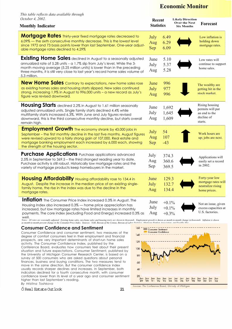
Monthly Indicator

Recent

Statistics

Likely Direction

Over the Next

Six MonthsForecast

Notes: All rates are seasonally adjusted. Existing home sales, new home sales and housing starts are shown in thousands. Employment growth is shown as month-to-month change in thousands. Inflation is shown

as month-to-month percent change in the Consumer Price Index. Sources: NAR, Bureau of the Census, Bureau of Labor Statistics, Mortgage Bankers Association, and Freddie Mac.

Economic Monitor

July

Aug

Sep

6.49

6.29

6.09

JuneJuly

Aug

5.105.37

5.28

June

July

Aug

996

977

996

June

July

Aug

1,692

1,6451,609

July

Aug

Sep

54

107

-43

374.3

360.6

369.5

129.3

132.7

134.4

+0.1%

+0.1%

+0.3%

This table reflects data available through

October 4, 2002.

21

Mortgage Rates Thirty-year fixed mortgage rates decreased to

6.09% — the sixth consecutive monthly decrease. This is the lowest level

since 1972 and 73 basis points lower than last September. One-year adjust-able mortgage rates declined to 4.29%

Low inflatio

holding dow

mortgage rat

Existing Home Sales declined in August to a seasonally adjusted

annualized rate of 5.28 units – a 1.7% slip from July’s level. While the 3-

month moving average (5.25 million units) is lower than in the precedingthree months, it is still very close to last year’s record home sales volume of

5.3 million.

Low rates wi

continue to su

home sales.

New Home Sales Contrary to expectations, new home sales rose

as existing homes sales and housing starts slipped. New sales continued

strong, increasing 1.9% in August to 996,000 units – a new record as July’sfigure was revised downward.

The wealthy a

getting hit in t

stock market.

Housing Starts declined 2.2% in August to 1.61 million seasonally

adjusted annualized units. Single family starts declined 4.4% while

multifamily starts increased 6.3%. With June and July figures reviseddownward, this is the third consecutive monthly decline, but starts overall

remain high.

Rising housin

permits will p

an end to the

decline of

starts.

Employment Growth The economy shrank by 43,000 jobs in

September – the first monthly decline in the last five months. August figureswere revised upward to a fairly strong gain of 107,000. Real estate and

mortgage banking employment each increased by 6,000 each, showingthe strength of the housing sector.

Work hours a

up; jobs are n

Purchase Applications Purchase applications advanced

2.5% in September to 369.5 – the third strongest reading year to date.

Purchase activity is still robust. Historically low mortgage rates and thevariety of mortgage products keep homebuyers in the market.

July

Aug

Sep

Applications

easily set a re

in 2002.

Housing Affordability Housing affordability rose to 134.4 in

August. Despite the increase in the median price of an existing single-family home, the rise in the index was due to the decline in the

mortgage rates.

Forty-year lo

mortgage rate

neutralize risi

home prices.

June

July

Aug

Inflation The Consumer Price Index increased 0.3% in August. The

Housing Index also increased 0.3% — home price appreciation hasincreased, but low mortgage rates have limited increases in monthly

payments. The core index (excluding Food and Energy) increased 0.3% aswell.

Consumer Confidence and SentimentConsumer Confidence and consumer sentiment, two measures of thedegree of comfort consumers feel in their employment and financialprospects, are very important determinants of short-run home salesactivity. The Consumer Confidence Index, published by theConference Board, evaluates how consumers feel about their presentsituation and future expectations. Consumer Sentiment, published bythe University of Michigan Consumer Research Center, is based on asurvey of 500 consumers who are asked questions about personalfinances, business and buying conditions. The two measures tend tomove in the same direction. But the consumer confidence indexusually records sharper declines and increases. In September, bothindicators declined for a fourth consecutive month, with consumer confidence lower than its level of a year ago and consumer sentimenthigher than last September’s reading.

By Hristina Toshkova

Not an issue,

excess capaci

U.S. factories

June

July

Aug