


Languages
Pages
Legal


1
Micro‐ and Meso‐scale modelling
6/11/2013 1CompositesIves De Baere and Joris Degrieck – 2013‐2014
Part Design
• Stiffness• Strength• Damage tolerance
F ti
Micro‐meso‐macro homogenization methods
Motivation
• Fatigue • Static
Experimental
6/11/2013 2CompositesIves De Baere and Joris Degrieck – 2013‐2014
Wednesday, 06 November 2013
Numerical

2
Textile compositesMotivation
Micro‐meso‐macro homogenization methods
UD composite
Fibre
Plain weave Twill weave
6/11/2013 3CompositesIves De Baere and Joris Degrieck – 2013‐2014
Satin weave 2D braided composite
Knitted composites etc..
Analytical Micro‐mechanical homogenization
6/11/2013 4CompositesIves De Baere and Joris Degrieck – 2013‐2014

3
• if the reinforcement consists of particles, elliptical inclusions or short fibres, homogenization methods exist for prediction of elastic moduli and thermal expansion coefficients
Micro‐mechanical homogenization of particle‐reinforced composites
• the most well‐known homogenization method is the Mori‐Tanaka method
• commercial implementations exist, amongst others, by e‐XstreamEngineering (Digimat software)
• mainly applied for short‐fibre composites
6/11/2013 5CompositesIves De Baere and Joris Degrieck – 2013‐2014
• analytical homogenization methods for spherical and elliptical inclusions fail for continuous fibres (much larger aspect ratios)
• analytical Rules of Mixture (ROM) are used instead
Micro‐mechanical homogenization of UD fibre‐reinforced composites
• analytical Rules of Mixture (ROM) are used instead
6/11/2013 6CompositesIves De Baere and Joris Degrieck – 2013‐2014
4
With volume fraction of the fibers
Physical properites: density
There is a direct link between the volume fraction and the mass fraction
fv
1m f vv v v
volume fraction of the matrix
volume fraction of the voids
. (1 )
f
f f mf f f
ff f v
m
Mm v v
M v v v
f
mv
vv
6/11/2013 7CompositesIves De Baere and Joris Degrieck – 2013‐2014
Remark: in literature, fibre volume fraction is often noted with capital Vf, to avoid mistaking it with the Possion’s ratio
.(1 )
m m mm m
ff v m
m
M vm v
M v v v
Representative volume element of unidirectional ply
stress taken by fibres and matrices average applied stress
Analytical Rules of Mixture (ROM) for UD composites
• Equilibrium in axial direction:
matrix
fibre
homogeneousmatrix
6/11/2013 8CompositesIves De Baere and Joris Degrieck – 2013‐2014
1 1 11 11 11
1
f f m m
f f m m
F W E W E W E
E V E V E
• Rule of Mixture requires elastic properties of fibre and matrix !
( W, Wf and Wm = surface areas, V, Vf and Vm = volume fractions !! )

5
Puck’s formulas are frequently used to estimate 4 (out of 5) elastic properties of the unidirectional ply. Puck’s formulas assume an isotropic matrix and an isotropic fibre (not true for carbon fibre !!!)
E G i t i fib ti
Analytical Rules of Mixture (ROM) for UD composites
11
12
2
221.25
(1 )
(1 )
1 0.85
(1 )
f f f m
f f f m
fm
mf f
f
E V E V E
V V
VE E
EV V
E
Ef, Gf en f = isotropic fibre properties,
Em, Gm en m = isotropic matrix properties,
Vf = 1 – Vm = fibre volume fraction
0
2(1 )f
ff
m
EG
EE
6/11/2013 9CompositesIves De Baere and Joris Degrieck – 2013‐2014
121.25
1 0.6
(1 )
f
mm
f ff
VG G
GV V
G
2
2(1 )
1m
mm
mm
m
E
GE
121 E
The formula by Foye provides an estimate of the fifth elastic property of a unidirectional ply
Analytical Rules of Mixture (ROM) for UD composites
123
2 12
1
1(1 )
1
m m
f f f m
m m m
EE
V VE
E
6/11/2013 10CompositesIves De Baere and Joris Degrieck – 2013‐2014

6
Other popular formulas for micro‐mechanical homogenization are the ones proposed by Chamis
Analytical Rules of Mixture (ROM) for UD composites
6/11/2013 11CompositesIves De Baere and Joris Degrieck – 2013‐2014
Analytical Rules of Mixture (ROM) for UD composites
6/11/2013 12CompositesIves De Baere and Joris Degrieck – 2013‐2014

7
Finite Element Micro‐mechanical homogenization
6/11/2013 13CompositesIves De Baere and Joris Degrieck – 2013‐2014
YARN(carbon)
COMPOSITE[MPa]
Finite element micro‐mechanical homogenization
MATRIX [MPa]
6/11/2013 14CompositesIves De Baere and Joris Degrieck – 2013‐2014
MATRIX(epoxy)
[MPa]

8
Implementation of Periodic Boundary Conditions (PBC) through node‐coupling constraints
Loading case: uniaxial strain xx
Finite element micro‐mechanical homogenization
Constraint equations: Δx
X1X2
oad g case u a a st a xx
N1N2
6/11/2013 15CompositesIves De Baere and Joris Degrieck – 2013‐2014
q
Δy = y2 – y1 = 0
Δz = z2 – z1 = 0ɛy, ɛz, γxy, γxy, γxy = 0
N2
Degrees of freedom (3) of each pair of nodes belonging to opposite faces of
Implementation of Periodic Boundary Conditions (PBC) through node‐coupling constraints
Finite element micro‐mechanical homogenization
Constraint equations:
Degrees of freedom (3) of each pair of nodes belonging to opposite faces of the RVE are constrained kinematically
h d ff d l d
0
0
xu x
v
w
6/11/2013 16CompositesIves De Baere and Joris Degrieck – 2013‐2014
with Δu, Δv, Δw = difference in displacement in every directionΔx, Δy, Δz = difference in coordinates in every directionɛx, ɛy, ɛz, γxy, γxy, γxy = far‐field applied strains
9
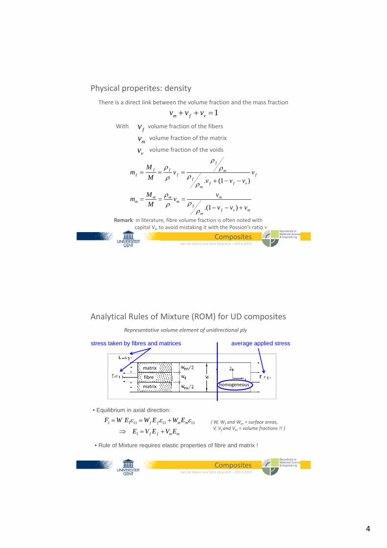
Finite element micro‐mechanical homogenization
ij ijVdV
Homogenised stresses ijHomogenised strains ijOne model for every loading:
Model input Analysis output
Homogenised elastic constants Cij
ijij
j
or
P
S
1. 11 nonzero
2. 22 nonzero
3. 33 nonzero
4. 12 nonzero
5. 23 nonzero
6. 13 nonzero
6/11/2013 17CompositesIves De Baere and Joris Degrieck – 2013‐2014
Finite element micro‐mechanical homogenization
48elements
4,400elements
36,320elements
4,410elements
6/11/2013 18CompositesIves De Baere and Joris Degrieck – 2013‐2014
[MPa] [MPa] [MPa][MPa]

10
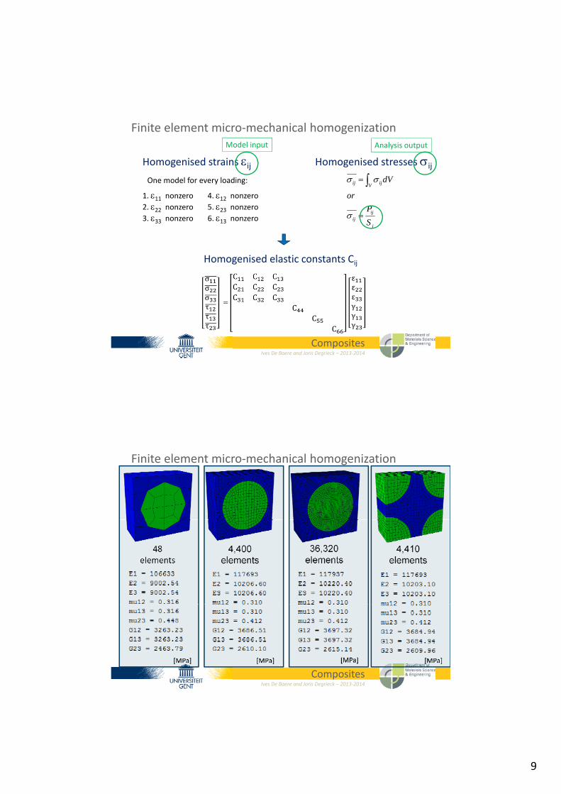
ORIGINAL MODEL ‘PERFECT BONDING’ ‘WEAK BONDING’
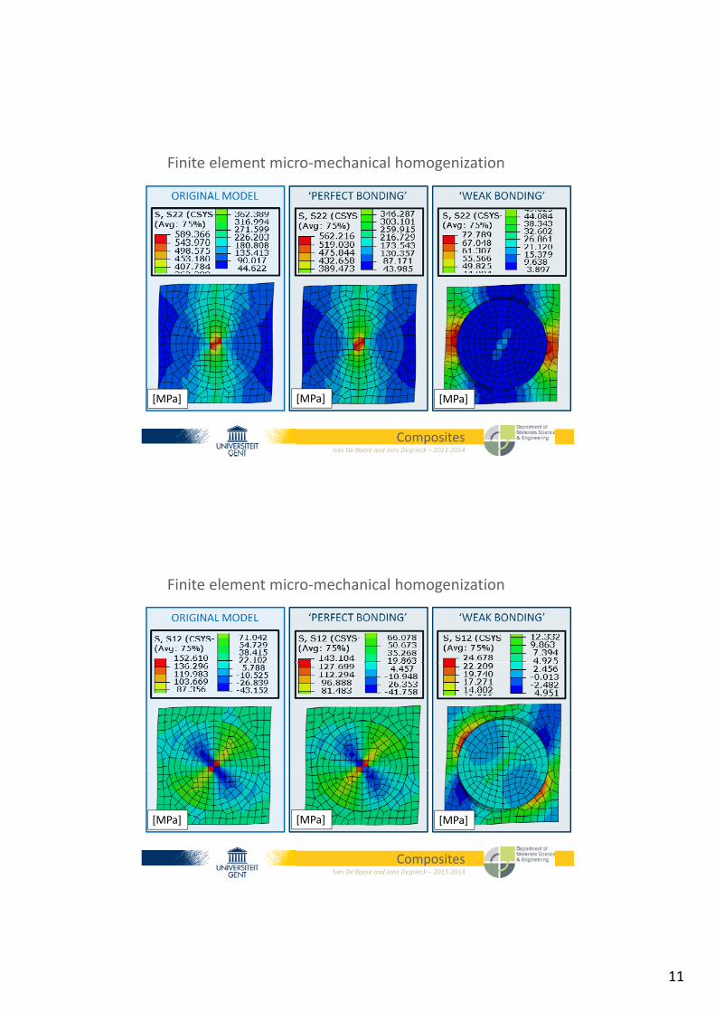
Finite element micro‐mechanical homogenization
yarnmatrixno cohesive layer
yarnmatrixstiff cohesive layer
yarnmatrixsoft cohesive layer
6/11/2013 19CompositesIves De Baere and Joris Degrieck – 2013‐2014
E = 1000 MPa G1 = 1000 MPa G2 = 1000 MPa
E = 10E6 MPa G1 = 10E6 MPa G2 = 10E6 MPa
perfect bonding by definition
3D periodic boundary conditions
εy
Finite element micro‐mechanical homogenization
γxy
6/11/2013 20CompositesIves De Baere and Joris Degrieck – 2013‐2014
εy = γxy = 1%
11
ORIGINAL MODEL ‘PERFECT BONDING’ ‘WEAK BONDING’
Finite element micro‐mechanical homogenization
6/11/2013 21CompositesIves De Baere and Joris Degrieck – 2013‐2014
[MPa] [MPa][MPa]
ORIGINAL MODEL ‘PERFECT BONDING’ ‘WEAK BONDING’
Finite element micro‐mechanical homogenization
6/11/2013 22CompositesIves De Baere and Joris Degrieck – 2013‐2014
[MPa] [MPa][MPa]
12
Finite Element Meso‐mechanical homogenization
6/11/2013 23CompositesIves De Baere and Joris Degrieck – 2013‐2014
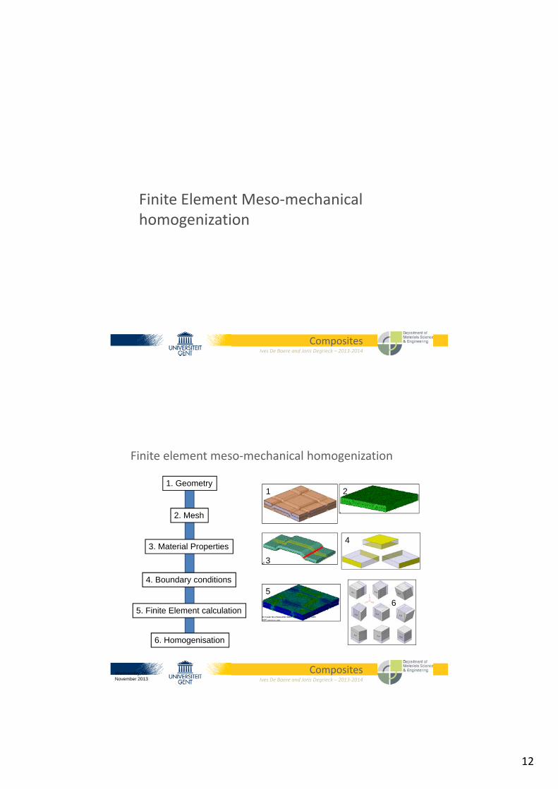
1. Geometry
2 Mesh
1 2
Finite element meso‐mechanical homogenization
2. Mesh
3. Material Properties
4. Boundary conditions
3
5
4
6
6/11/2013 24CompositesIves De Baere and Joris Degrieck – 2013‐2014
Wednesday, 06 November 2013
6. Homogenisation
5. Finite Element calculation6

13
FE -Abaqus ***Micro-CT Catia V5 ***
Finite element meso‐mechanical homogenization
PBC Creator
Homogenization (Chamis)
FE l l ti Homogenized Properties
Local Material Orientations
6/11/2013 25CompositesIves De Baere and Joris Degrieck – 2013‐2014
Wednesday, 06 November 2013
FE calculations
Macro homogenization
Homogenized Properties
Composite material under study (Ten Cate)• 5‐harness satin weave carbon fabric‐reinforced PPS (Vf = 50 %)• [(0°,90°)]4s stacking sequence: 8 layers of
(0° 90°) fabric
Illustration of procedure for textile composite
(0 ,90 ) fabric• Composite plates were hot pressed
310 °C and 10 bar• CETEX : 6 tons in Airbus A380
6/11/2013 26CompositesIves De Baere and Joris Degrieck – 2013‐2014

14
Illustration of procedure for textile composite
6/11/2013 27CompositesIves De Baere and Joris Degrieck – 2013‐2014
7.4mm
Illustration of procedure for textile composite
6/11/2013 28CompositesIves De Baere and Joris Degrieck – 2013‐2014
15
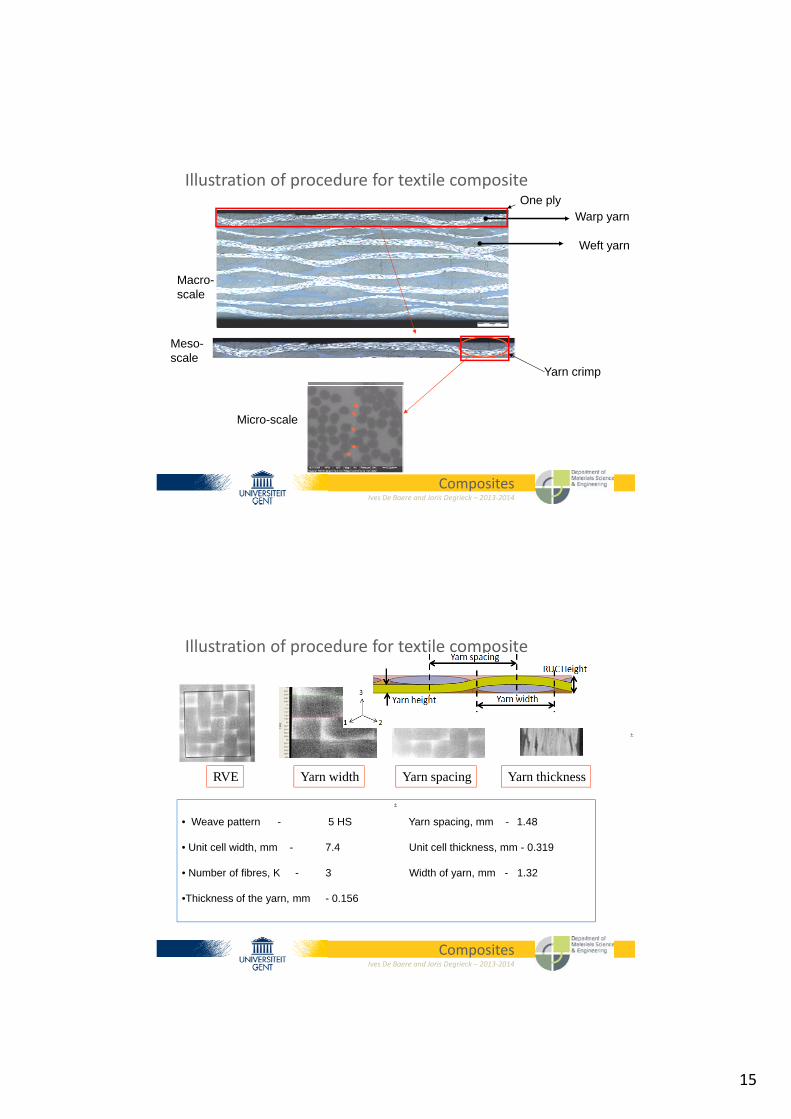
Warp yarn
Weft yarn
One ply
Illustration of procedure for textile composite
Yarn crimp
Macro-scale
Meso-scale
6/11/2013 29CompositesIves De Baere and Joris Degrieck – 2013‐2014
Micro-scale
Illustration of procedure for textile composite
RVE Yarn width Yarn thicknessYarn spacing
• Weave pattern - 5 HS Yarn spacing, mm - 1.48
• Unit cell width, mm - 7.4 Unit cell thickness, mm - 0.319
6/11/2013 30CompositesIves De Baere and Joris Degrieck – 2013‐2014
, ,
• Number of fibres, K - 3 Width of yarn, mm - 1.32
•Thickness of the yarn, mm - 0.156

16
Meshing arbitrary 3D yarns with correct local material orientations
Illustration of procedure for textile composite
6/11/2013 31CompositesIves De Baere and Joris Degrieck – 2013‐2014
Illustration of procedure for textile composite
6/11/2013 32CompositesIves De Baere and Joris Degrieck – 2013‐2014

17
DONE Cohesive elements – applications
3D periodic boundary conditions
Illustration of procedure for textile composite
6/11/2013 33CompositesIves De Baere and Joris Degrieck – 2013‐2014
εx = 0,5%
MethodE11
[GPa]
E22
[GPa]
E33
[GPa]
23
G12
[MPa]
G13
[MPa]
G23
[MPa]
Illustration of procedure for textile composite
[GPa] [GPa] [GPa] [MPa] [MPa] [MPa]
Periodic BCs & volume averaging
56.49 56.41 10.53 0.08 0.41 0.41 4280 3048 3045
Experiment 57.0 57.0 - 0.05 - - 4175 - -
6/11/2013 34CompositesIves De Baere and Joris Degrieck – 2013‐2014
Wednesday, 06 November 2013
This sheet is property of Stefan Jacques and shall not be copied or disclosed to a third party without a written authorization

18
Illustration of procedure for textile composite
6/11/2013 35CompositesIves De Baere and Joris Degrieck – 2013‐2014
Max strain Min strainAverage strainIllustration of procedure for textile composite
6/11/2013 36CompositesIves De Baere and Joris Degrieck – 2013‐2014

19
Illustration of procedure for textile composite
6/11/2013 37CompositesIves De Baere and Joris Degrieck – 2013‐2014
Top Related