


Languages
Pages
Legal

Machine LearningLecture 7: SVM
Moshe KoppelSlides adapted from Andrew Moore
Copyright © 2001, 2003, Andrew W. Moore

Nov 23rd, 2001Copyright © 2001, 2003, Andrew W. Moore
Support Vector Machines
Andrew W. MooreProfessor
School of Computer ScienceCarnegie Mellon University
www.cs.cmu.edu/[email protected]
412-268-7599
Note to other teachers and users of these slides. Andrew would be delighted if you found this source material useful in giving your own lectures. Feel free to use these slides verbatim, or to modify them to fit your own needs. PowerPoint originals are available. If you make use of a significant portion of these slides in your own lecture, please include this message, or the following link to the source repository of Andrew’s tutorials: http://www.cs.cmu.edu/~awm/tutorials . Comments and corrections gratefully received.

Support Vector Machines: Slide 3Copyright © 2001, 2003, Andrew W. Moore
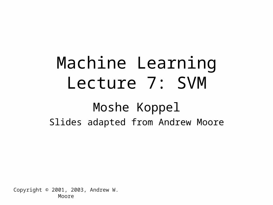
Linear Classifiers
f x
yest
denotes +1
denotes -1
f(x,w,b) = sign(w. x - b)
How would you classify this data?
Support Vector Machines: Slide 4Copyright © 2001, 2003, Andrew W. Moore
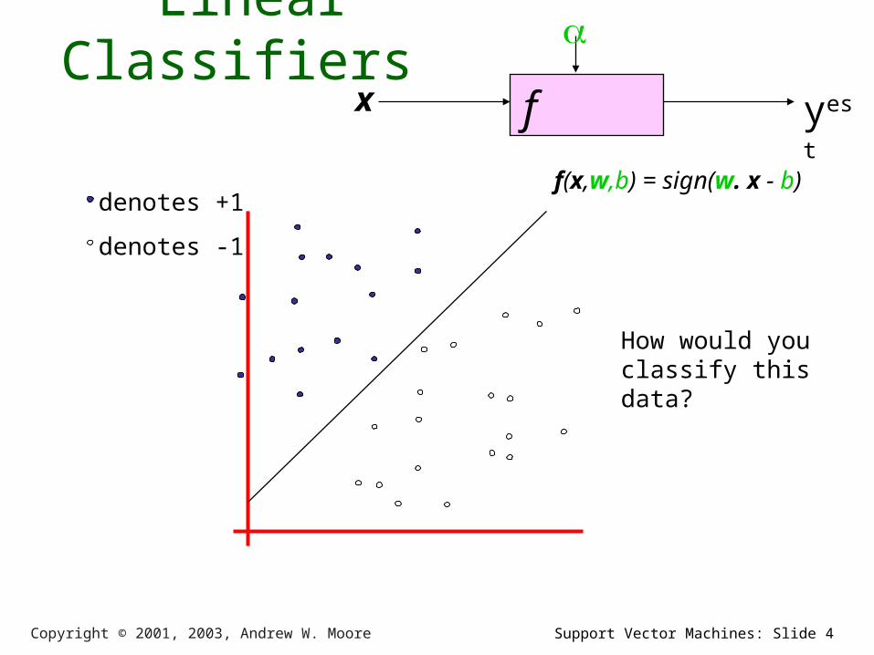
Linear Classifiers
f x
yest
denotes +1
denotes -1
f(x,w,b) = sign(w. x - b)
How would you classify this data?
Support Vector Machines: Slide 5Copyright © 2001, 2003, Andrew W. Moore
Linear Classifiers
f x
yest
denotes +1
denotes -1
f(x,w,b) = sign(w. x - b)
How would you classify this data?

Support Vector Machines: Slide 6Copyright © 2001, 2003, Andrew W. Moore
Linear Classifiers
f x
yest
denotes +1
denotes -1
f(x,w,b) = sign(w. x - b)
How would you classify this data?
Support Vector Machines: Slide 7Copyright © 2001, 2003, Andrew W. Moore
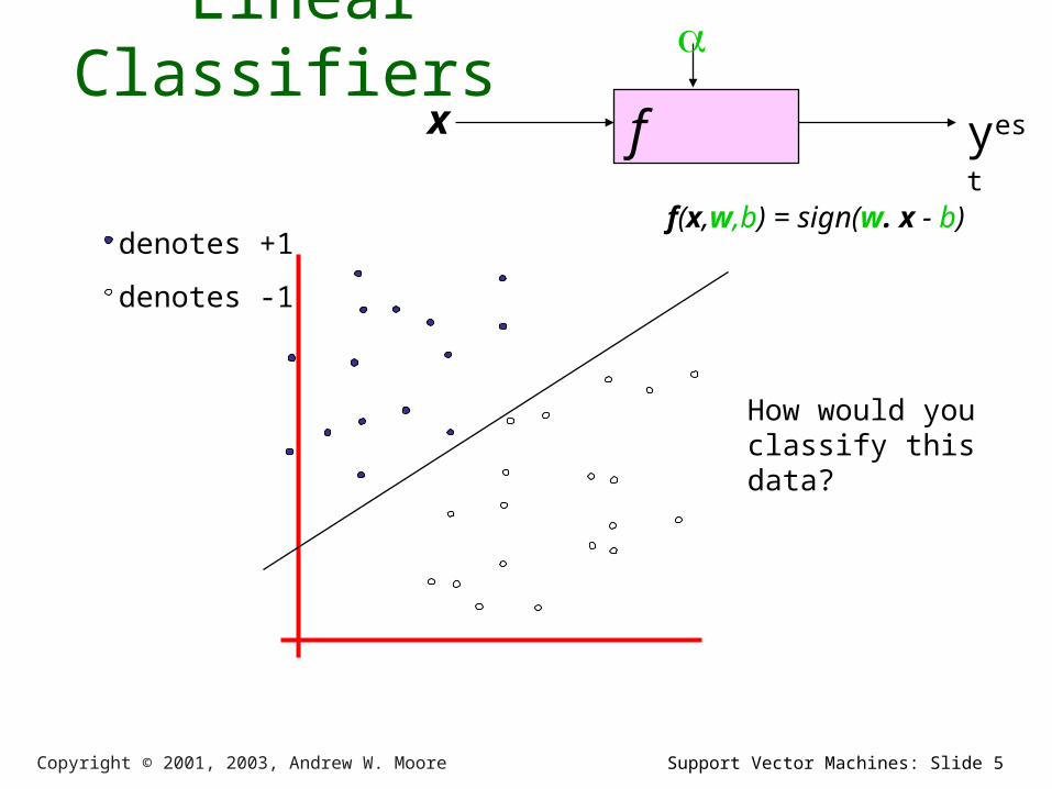
Linear Classifiers
f x
yest
denotes +1
denotes -1
f(x,w,b) = sign(w. x - b)
Any of these would be fine..
..but which is best?
Support Vector Machines: Slide 8Copyright © 2001, 2003, Andrew W. Moore
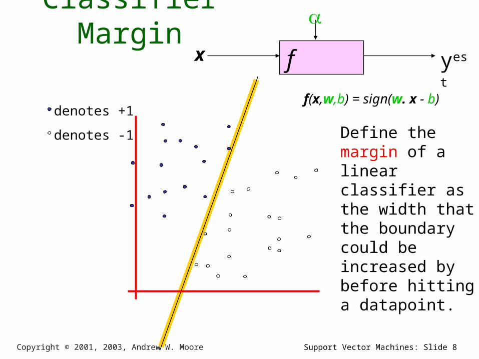
Classifier Margin
f x
yest
denotes +1
denotes -1
f(x,w,b) = sign(w. x - b)
Define the margin of a linear classifier as the width that the boundary could be increased by before hitting a datapoint.
Support Vector Machines: Slide 9Copyright © 2001, 2003, Andrew W. Moore
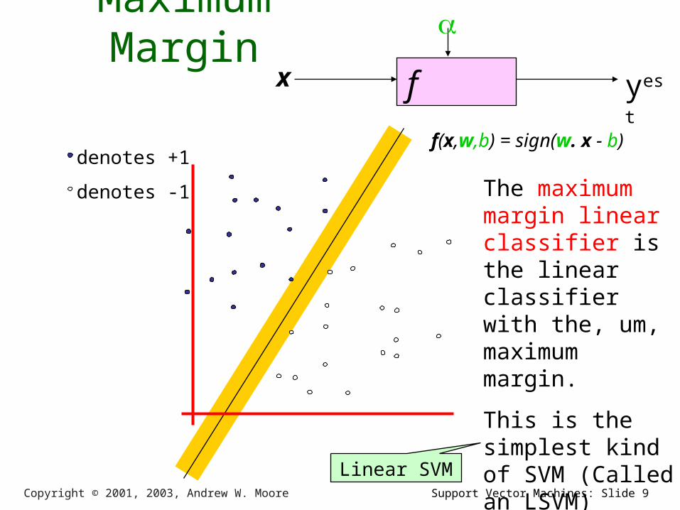
Maximum Margin
f x
yest
denotes +1
denotes -1
f(x,w,b) = sign(w. x - b)
The maximum margin linear classifier is the linear classifier with the, um, maximum margin.
This is the simplest kind of SVM (Called an LSVM)Linear SVM
Support Vector Machines: Slide 10Copyright © 2001, 2003, Andrew W. Moore
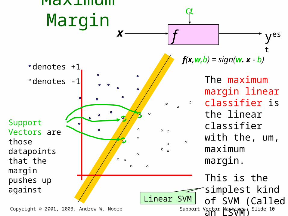
Maximum Margin
f x
yest
denotes +1
denotes -1
f(x,w,b) = sign(w. x - b)
The maximum margin linear classifier is the linear classifier with the, um, maximum margin.
This is the simplest kind of SVM (Called an LSVM)
Support Vectors are those datapoints that the margin pushes up against
Linear SVM
Support Vector Machines: Slide 11Copyright © 2001, 2003, Andrew W. Moore
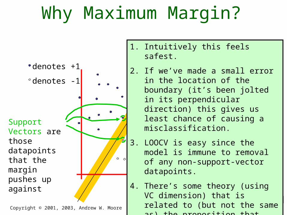
Why Maximum Margin?
denotes +1
denotes -1
f(x,w,b) = sign(w. x - b)
The maximum margin linear classifier is the linear classifier with the, um, maximum margin.
This is the simplest kind of SVM (Called an LSVM)
Support Vectors are those datapoints that the margin pushes up against
1. Intuitively this feels safest.
2. If we’ve made a small error in the location of the boundary (it’s been jolted in its perpendicular direction) this gives us least chance of causing a misclassification.
3. LOOCV is easy since the model is immune to removal of any non-support-vector datapoints.
4. There’s some theory (using VC dimension) that is related to (but not the same as) the proposition that this is a good thing.
5. Empirically it works very very well.
Support Vector Machines: Slide 12Copyright © 2001, 2003, Andrew W. Moore
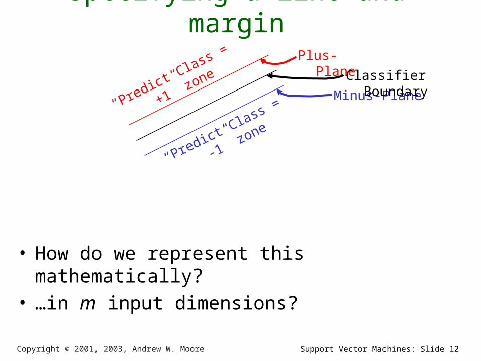
Specifying a line and margin
• How do we represent this mathematically?• …in m input dimensions?
Plus-Plane
Minus-Plane
Classifier Boundary
“Predict Class
= +1”
zone
“Predict Class
= -1”
zone
Support Vector Machines: Slide 13Copyright © 2001, 2003, Andrew W. Moore
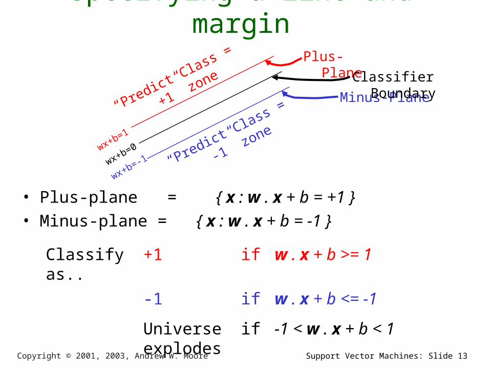
Specifying a line and margin
• Plus-plane = { x : w . x + b = +1 }• Minus-plane = { x : w . x + b = -1 }
Plus-Plane
Minus-Plane
Classifier Boundary
“Predict Class
= +1”
zone
“Predict Class
= -1”
zone
Classify as..
+1 if w . x + b >= 1
-1 if w . x + b <= -1
Universe explodes
if -1 < w . x + b < 1
wx+b=1
wx+b=0
wx+b=-
1

Support Vector Machines: Slide 14Copyright © 2001, 2003, Andrew W. Moore
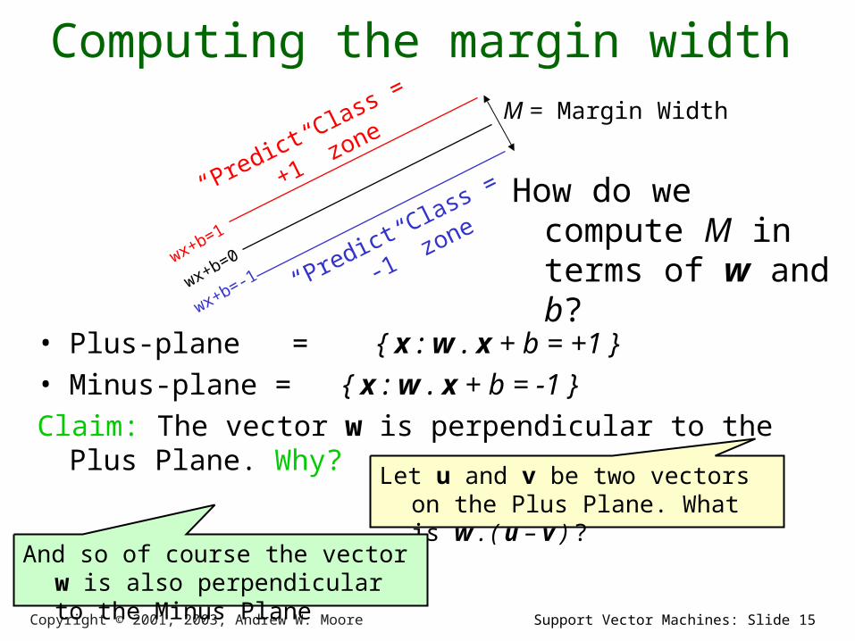
Computing the margin width
• Plus-plane = { x : w . x + b = +1 }• Minus-plane = { x : w . x + b = -1 }Claim: The vector w is perpendicular to the Plus Plane.
Why?
“Predict Class
= +1”
zone
“Predict Class
= -1”
zonewx+b=1
wx+b=0
wx+b=-
1
M = Margin Width
How do we compute M in terms of w and b?
Support Vector Machines: Slide 15Copyright © 2001, 2003, Andrew W. Moore
Computing the margin width
• Plus-plane = { x : w . x + b = +1 }• Minus-plane = { x : w . x + b = -1 }Claim: The vector w is perpendicular to the Plus Plane.
Why?
“Predict Class
= +1”
zone
“Predict Class
= -1”
zonewx+b=1
wx+b=0
wx+b=-
1
M = Margin Width
How do we compute M in terms of w and b?
Let u and v be two vectors on the Plus Plane. What is w . ( u – v ) ?
And so of course the vector w is also perpendicular to the Minus Plane
Support Vector Machines: Slide 16Copyright © 2001, 2003, Andrew W. Moore
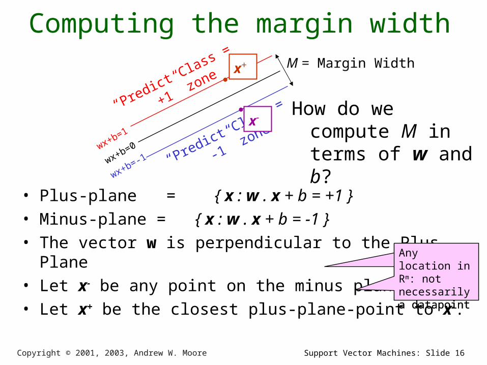
Computing the margin width
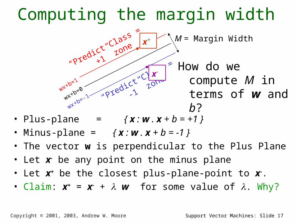
• Plus-plane = { x : w . x + b = +1 }• Minus-plane = { x : w . x + b = -1 }• The vector w is perpendicular to the Plus Plane• Let x- be any point on the minus plane• Let x+ be the closest plus-plane-point to x-.
“Predict Class
= +1”
zone
“Predict Class
= -1”
zonewx+b=1
wx+b=0
wx+b=-
1
M = Margin Width
How do we compute M in terms of w and b?
x-
x+
Any location in m: not necessarily a datapoint
Any location in Rm: not necessarily a datapoint
Support Vector Machines: Slide 17Copyright © 2001, 2003, Andrew W. Moore
Computing the margin width
• Plus-plane = { x : w . x + b = +1 }• Minus-plane = { x : w . x + b = -1 }• The vector w is perpendicular to the Plus Plane• Let x- be any point on the minus plane• Let x+ be the closest plus-plane-point to x-.• Claim: x+ = x- + w for some value of . Why?
“Predict Class
= +1”
zone
“Predict Class
= -1”
zonewx+b=1
wx+b=0
wx+b=-
1
M = Margin Width
How do we compute M in terms of w and b?
x-
x+
Support Vector Machines: Slide 18Copyright © 2001, 2003, Andrew W. Moore
Computing the margin width
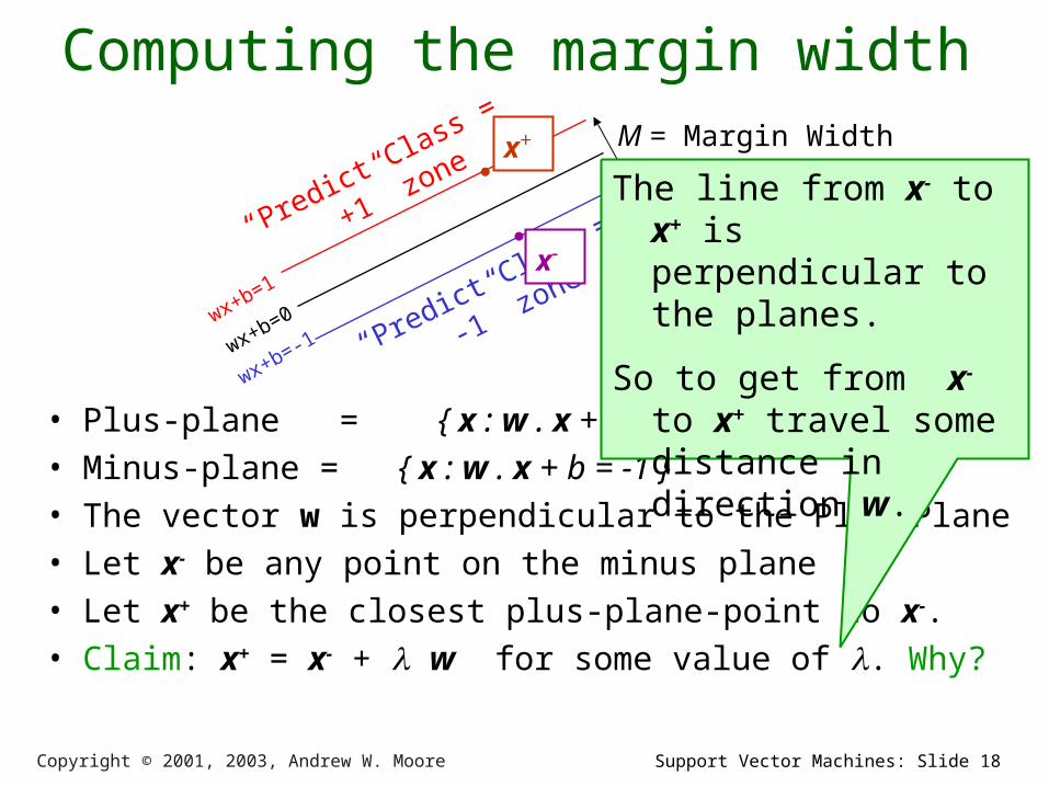
• Plus-plane = { x : w . x + b = +1 }• Minus-plane = { x : w . x + b = -1 }• The vector w is perpendicular to the Plus Plane• Let x- be any point on the minus plane• Let x+ be the closest plus-plane-point to x-.• Claim: x+ = x- + w for some value of . Why?
“Predict Class
= +1”
zone
“Predict Class
= -1”
zonewx+b=1
wx+b=0
wx+b=-
1
M = Margin Width
How do we compute M in terms of w and b?
x-
x+
The line from x- to x+ is perpendicular to the planes.
So to get from x- to x+ travel some distance in direction w.
Support Vector Machines: Slide 19Copyright © 2001, 2003, Andrew W. Moore
Computing the margin width
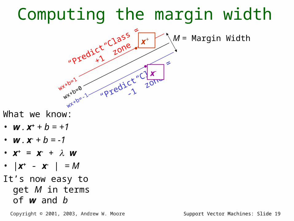
What we know:• w . x+ + b = +1 • w . x- + b = -1 • x+ = x- + w• |x+ - x- | = MIt’s now easy to get
M in terms of w and b
“Predict Class
= +1”
zone
“Predict Class
= -1”
zonewx+b=1
wx+b=0
wx+b=-
1
M = Margin Width
x-
x+

Support Vector Machines: Slide 20Copyright © 2001, 2003, Andrew W. Moore
Computing the margin width
What we know:• w . x+ + b = +1 • w . x- + b = -1 • x+ = x- + w• |x+ - x- | = MIt’s now easy to get
M in terms of w and b
“Predict Class
= +1”
zone
“Predict Class
= -1”
zonewx+b=1
wx+b=0
wx+b=-
1
M = Margin Width
w . (x - + w) + b = 1
=>
w . x - + b + w .w = 1
=>
-1 + w .w = 1
=>
x-
x+
w.w
2λ

Support Vector Machines: Slide 21Copyright © 2001, 2003, Andrew W. Moore
Computing the margin width
What we know:• w . x+ + b = +1 • w . x- + b = -1 • x+ = x- + w• |x+ - x- | = M•
“Predict Class
= +1”
zone
“Predict Class
= -1”
zonewx+b=1
wx+b=0
wx+b=-
1
M = Margin Width =
M = |x+ - x- | =| w |=
x-
x+
w.w
2λ
wwww
ww
.
2
.
.2
www .|| λλ
ww.
2
Support Vector Machines: Slide 22Copyright © 2001, 2003, Andrew W. Moore
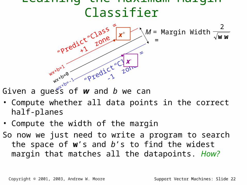
Learning the Maximum Margin Classifier
Given a guess of w and b we can• Compute whether all data points in the correct half-
planes• Compute the width of the marginSo now we just need to write a program to search the
space of w’s and b’s to find the widest margin that matches all the datapoints. How?
“Predict Class
= +1”
zone
“Predict Class
= -1”
zonewx+b=1
wx+b=0
wx+b=-
1
M = Margin Width =
x-
x+ww.
2
Support Vector Machines: Slide 23Copyright © 2001, 2003, Andrew W. Moore
Learning via Quadratic Programming
• QP is a well-studied class of optimization algorithms to maximize a quadratic function of some real-valued variables subject to linear constraints.
Support Vector Machines: Slide 24Copyright © 2001, 2003, Andrew W. Moore
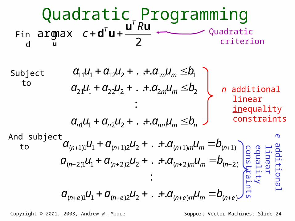
Quadratic Programming
2maxarg
uuud
u
Rc
TT Find
nmnmnn
mm
mm
buauaua
buauaua
buauaua
...
:
...
...
2211
22222121
11212111
)()(22)(11)(
)2()2(22)2(11)2(
)1()1(22)1(11)1(
...
:
...
...
enmmenenen
nmmnnn
nmmnnn
buauaua
buauaua
buauaua
And subject to
n additional linear inequality constraints
e a
dd
ition
al
linear
eq
uality
co
nstra
ints
Quadratic criterion
Subject to
Support Vector Machines: Slide 25Copyright © 2001, 2003, Andrew W. Moore
Quadratic Programming
2maxarg
uuud
u
Rc
TT Find
Subject to
nmnmnn
mm
mm
buauaua
buauaua
buauaua
...
:
...
...
2211
22222121
11212111
)()(22)(11)(
)2()2(22)2(11)2(
)1()1(22)1(11)1(
...
:
...
...
enmmenenen
nmmnnn
nmmnnn
buauaua
buauaua
buauaua
And subject to
n additional linear inequality constraints
e a
dd
ition
al
linear
eq
uality
co
nstra
ints
Quadratic criterion
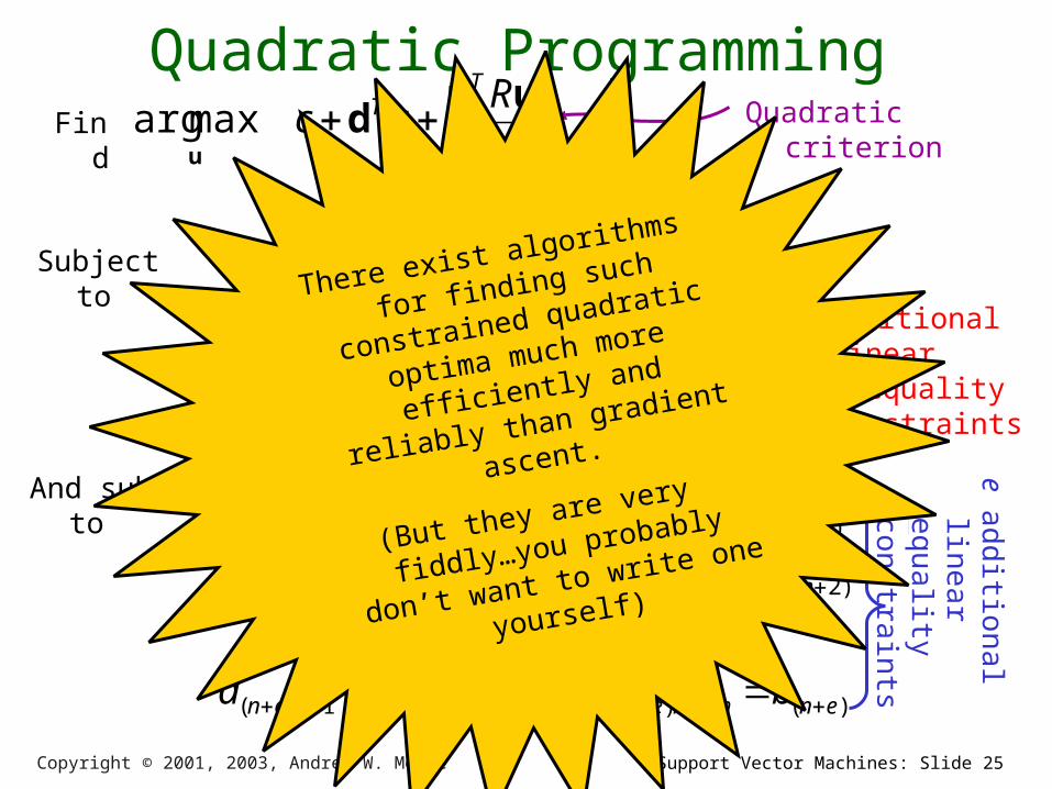
There exist algorithms for
finding such constrained
quadratic optima much
more efficiently and
reliably than gradient
ascent.
(But they are very fiddly…you
probably don’t want to
write one yourself)
Support Vector Machines: Slide 26Copyright © 2001, 2003, Andrew W. Moore
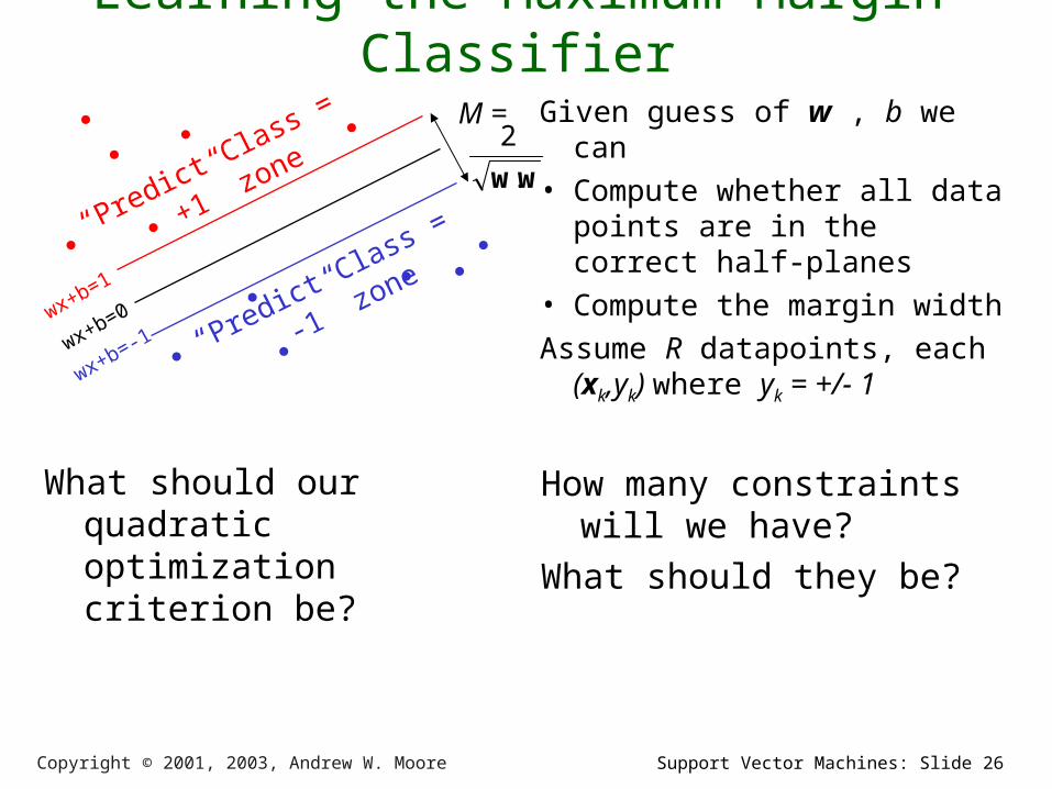
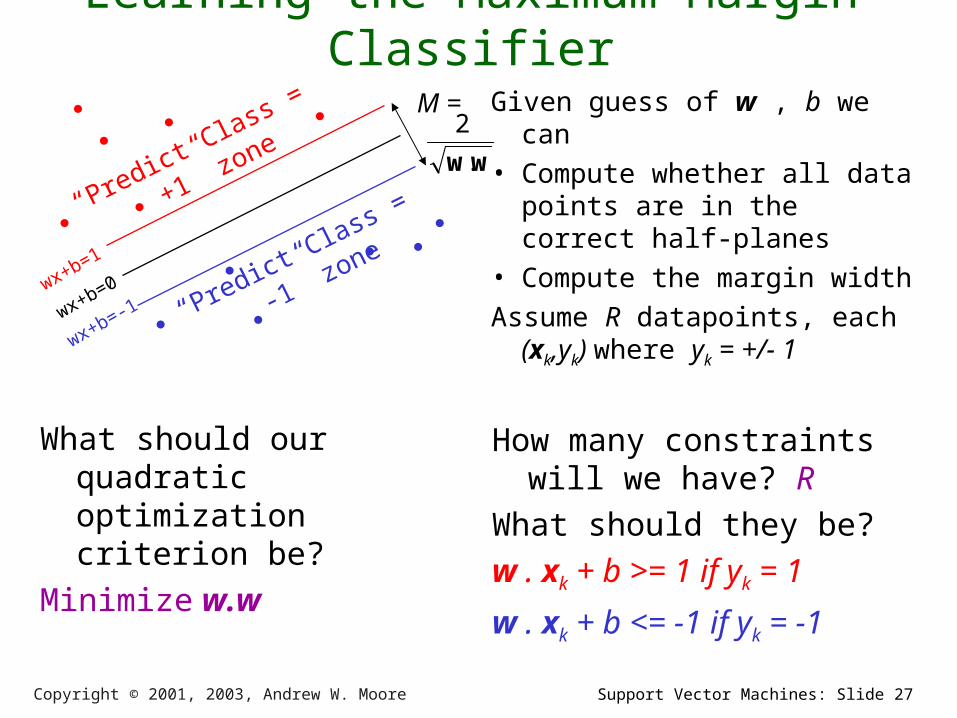
Learning the Maximum Margin Classifier
“Predict Class
= +1”
zone
“Predict Class
= -1”
zonewx+b=1
wx+b=0
wx+b=-
1
M =ww.
2
What should our quadratic optimization criterion be?
How many constraints will we have?
What should they be?
Given guess of w , b we can• Compute whether all data
points are in the correct half-planes
• Compute the margin widthAssume R datapoints, each
(xk,yk) where yk = +/- 1
Support Vector Machines: Slide 27Copyright © 2001, 2003, Andrew W. Moore
Learning the Maximum Margin Classifier
Given guess of w , b we can• Compute whether all data
points are in the correct half-planes
• Compute the margin widthAssume R datapoints, each
(xk,yk) where yk = +/- 1
“Predict Class
= +1”
zone
“Predict Class
= -1”
zonewx+b=1
wx+b=0
wx+b=-
1
M =ww.
2
What should our quadratic optimization criterion be?
Minimize w.w
How many constraints will we have? R
What should they be?w . xk + b >= 1 if yk = 1
w . xk + b <= -1 if yk = -1
Support Vector Machines: Slide 28Copyright © 2001, 2003, Andrew W. Moore
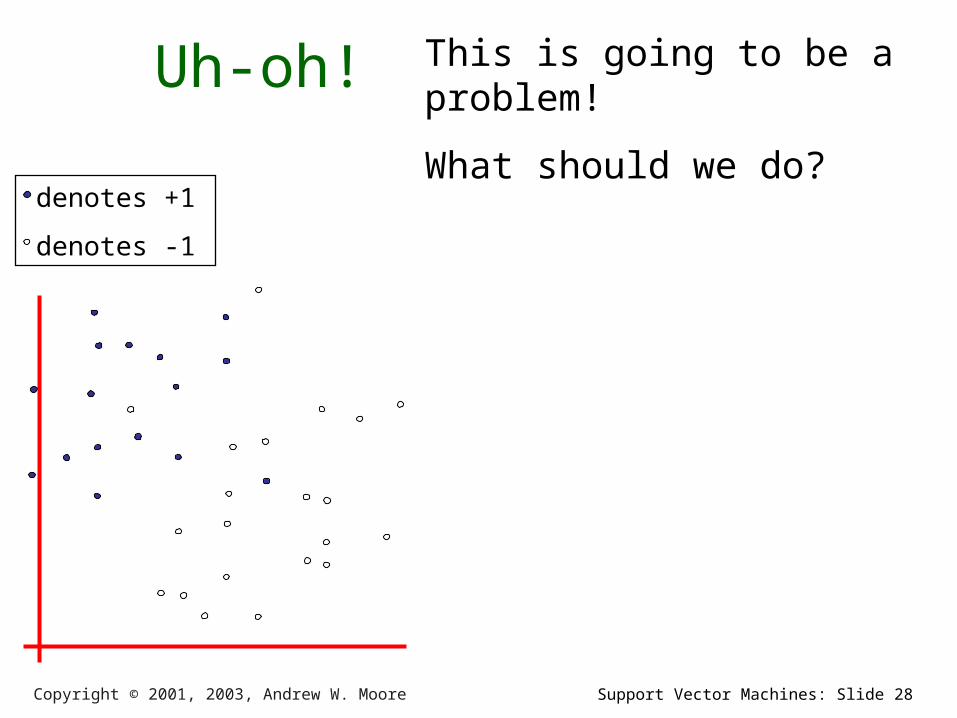
Uh-oh!
denotes +1
denotes -1
This is going to be a problem!
What should we do?

Support Vector Machines: Slide 29Copyright © 2001, 2003, Andrew W. Moore
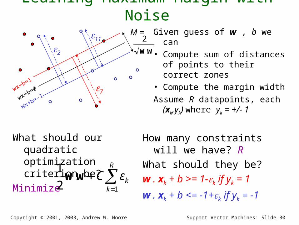
Learning Maximum Margin with Noise
Given guess of w , b we can• Compute sum of distances
of points to their correct zones
• Compute the margin widthAssume R datapoints, each
(xk,yk) where yk = +/- 1
wx+b=1
wx+b=0
wx+b=-
1
M =ww.
2
What should our quadratic optimization criterion be?
How many constraints will we have?
What should they be?
Support Vector Machines: Slide 30Copyright © 2001, 2003, Andrew W. Moore
Learning Maximum Margin with Noise
Given guess of w , b we can• Compute sum of distances
of points to their correct zones
• Compute the margin widthAssume R datapoints, each
(xk,yk) where yk = +/- 1
wx+b=1
wx+b=0
wx+b=-
1
M =ww.
2
What should our quadratic optimization criterion be?
Minimize
R
kkεC
1
.2
1ww
7
11 2
How many constraints will we have? R
What should they be?w . xk + b >= 1-k if yk = 1
w . xk + b <= -1+k if yk = -1

Support Vector Machines: Slide 31Copyright © 2001, 2003, Andrew W. Moore
Learning Maximum Margin with Noise
Given guess of w , b we can• Compute sum of distances
of points to their correct zones
• Compute the margin widthAssume R datapoints, each
(xk,yk) where yk = +/- 1
wx+b=1
wx+b=0
wx+b=-
1
M =ww.
2
What should our quadratic optimization criterion be?
Minimize
R
kkεC
1
.2
1ww
7
11 2
Our original (noiseless data) QP had m+1 variables: w1, w2, … wm, and b.
Our new (noisy data) QP has m+1+R variables: w1, w2, … wm, b, k , 1 ,… R
m = # input dimension
s
How many constraints will we have? R
What should they be?w . xk + b >= 1-k if yk = 1
w . xk + b <= -1+k if yk = -1
R= # records
Support Vector Machines: Slide 32Copyright © 2001, 2003, Andrew W. Moore
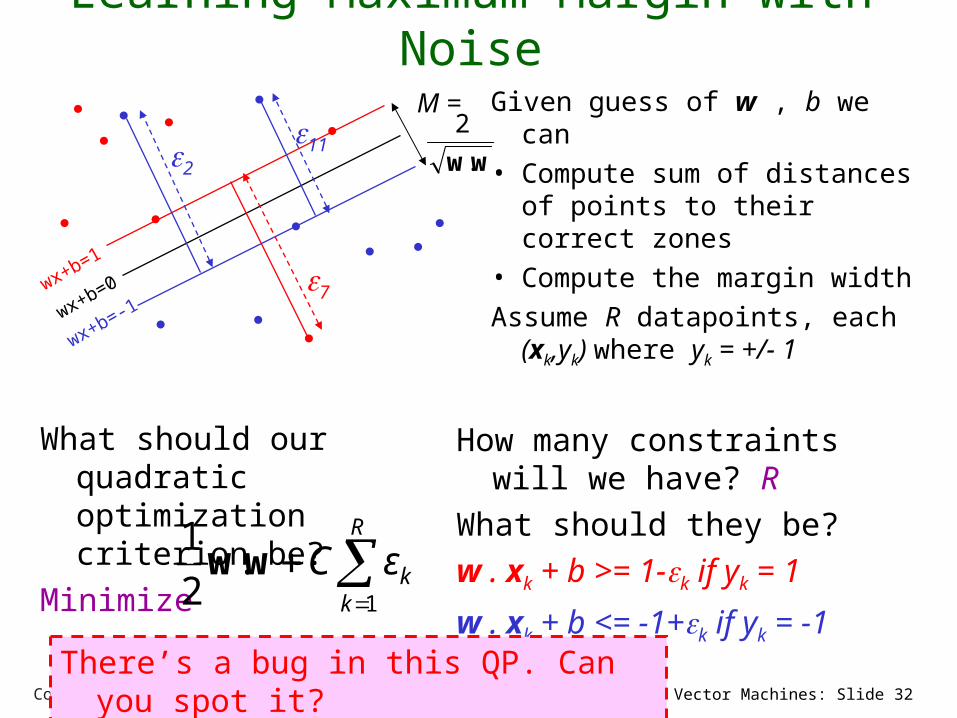
How many constraints will we have? R
What should they be?w . xk + b >= 1-k if yk = 1
w . xk + b <= -1+k if yk = -1
Learning Maximum Margin with Noise
Given guess of w , b we can• Compute sum of distances
of points to their correct zones
• Compute the margin widthAssume R datapoints, each
(xk,yk) where yk = +/- 1
wx+b=1
wx+b=0
wx+b=-
1
M =ww.
2
What should our quadratic optimization criterion be?
Minimize
R
kkεC
1
.2
1ww
7
11 2
There’s a bug in this QP. Can you spot it?

Support Vector Machines: Slide 33Copyright © 2001, 2003, Andrew W. Moore
Learning Maximum Margin with Noise
Given guess of w , b we can• Compute sum of distances
of points to their correct zones
• Compute the margin widthAssume R datapoints, each
(xk,yk) where yk = +/- 1
wx+b=1
wx+b=0
wx+b=-
1
M =ww.
2
What should our quadratic optimization criterion be?
Minimize
How many constraints will we have? 2R
What should they be?w . xk + b >= 1-k if yk = 1
w . xk + b <= -1+k if yk = -1
k >= 0 for all k
R
kkεC
1
.2
1ww
7
11 2
Support Vector Machines: Slide 34Copyright © 2001, 2003, Andrew W. Moore
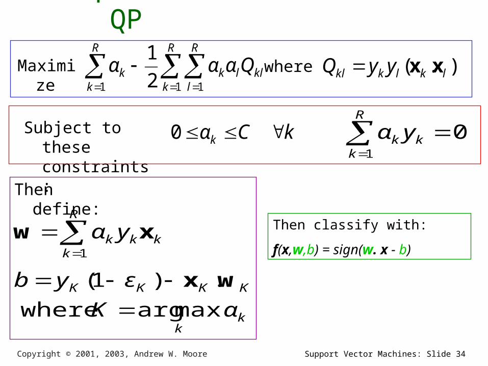
An Equivalent QP
Maximize
R
k
R
lkllk
R
kk Qααα
1 11 2
1where ).( lklkkl yyQ xx
Subject to these constraints:
kCαk 0
Then define:
R
kkkk yα
1
xw
kk
KKKK
αK
εyb
maxarg where
.)1(
wx
Then classify with:
f(x,w,b) = sign(w. x - b)
01
R
kkk yα

Support Vector Machines: Slide 35Copyright © 2001, 2003, Andrew W. Moore
An Equivalent QPMaximi
zewhere ).( lklkkl yyQ xx
Subject to these constraints:
kCαk 0
Then define:
R
kkkk yα
1
xw
kk
KKKK
αK
εyb
maxarg where
.)1(
wx
Then classify with:
f(x,w,b) = sign(w. x - b)
01
R
kkk yα
Datapoints with k > 0 will be the support vectors
..so this sum only needs to be over the support vectors.
R
k
R
lkllk
R
kk Qααα
1 11 2
1
Support Vector Machines: Slide 36Copyright © 2001, 2003, Andrew W. Moore
R
k
R
lkllk
R
kk Qααα
1 11 2
1An Equivalent QP
Maximize
where ).( lklkkl yyQ xx
Subject to these constraints:
kCαk 0
Then define:
R
kkkk yα
1
xw
kk
KKKK
αK
εyb
maxarg where
.)1(
wx
Then classify with:
f(x,w,b) = sign(w. x - b)
01
R
kkk yα
Datapoints with k > 0 will be the support vectors
..so this sum only needs to be over the support vectors.
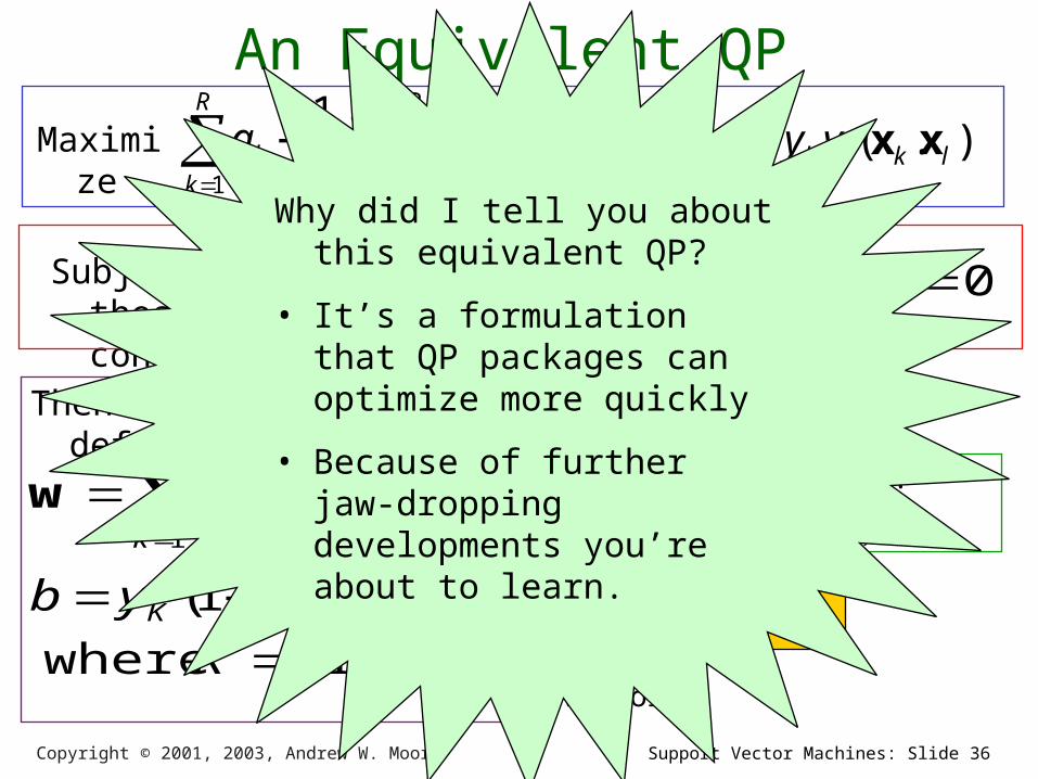
Why did I tell you about this equivalent QP?
• It’s a formulation that QP packages can optimize more quickly
• Because of further jaw-dropping developments you’re about to learn.
Support Vector Machines: Slide 37Copyright © 2001, 2003, Andrew W. Moore
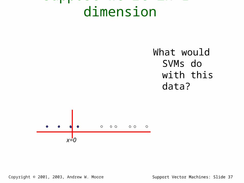
Suppose we’re in 1-dimension
What would SVMs do with this data?
x=0
Support Vector Machines: Slide 38Copyright © 2001, 2003, Andrew W. Moore
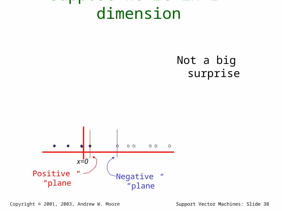
Suppose we’re in 1-dimension
Not a big surprise
Positive “plane” Negative “plane”
x=0
Support Vector Machines: Slide 39Copyright © 2001, 2003, Andrew W. Moore
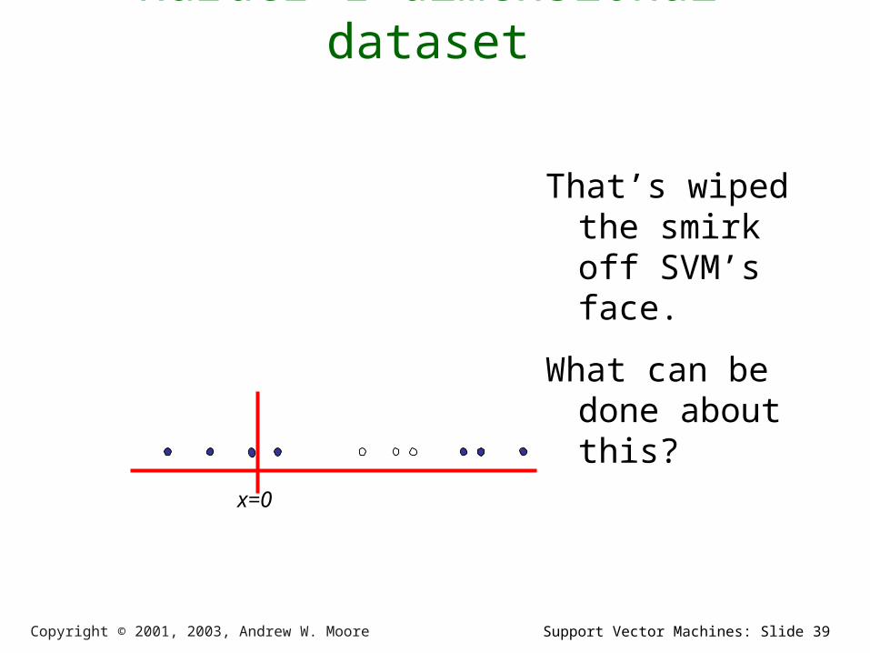
Harder 1-dimensional dataset
That’s wiped the smirk off SVM’s face.
What can be done about this?
x=0
Support Vector Machines: Slide 40Copyright © 2001, 2003, Andrew W. Moore
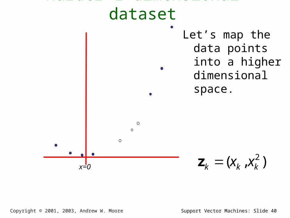
Harder 1-dimensional datasetLet’s map the
data points into a higher dimensional space.
x=0 ),( 2kkk xxz
Support Vector Machines: Slide 41Copyright © 2001, 2003, Andrew W. Moore
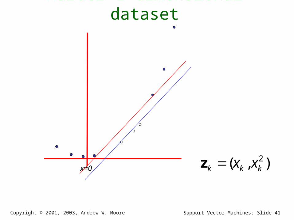
Harder 1-dimensional dataset
x=0 ),( 2kkk xxz
Support Vector Machines: Slide 42Copyright © 2001, 2003, Andrew W. Moore
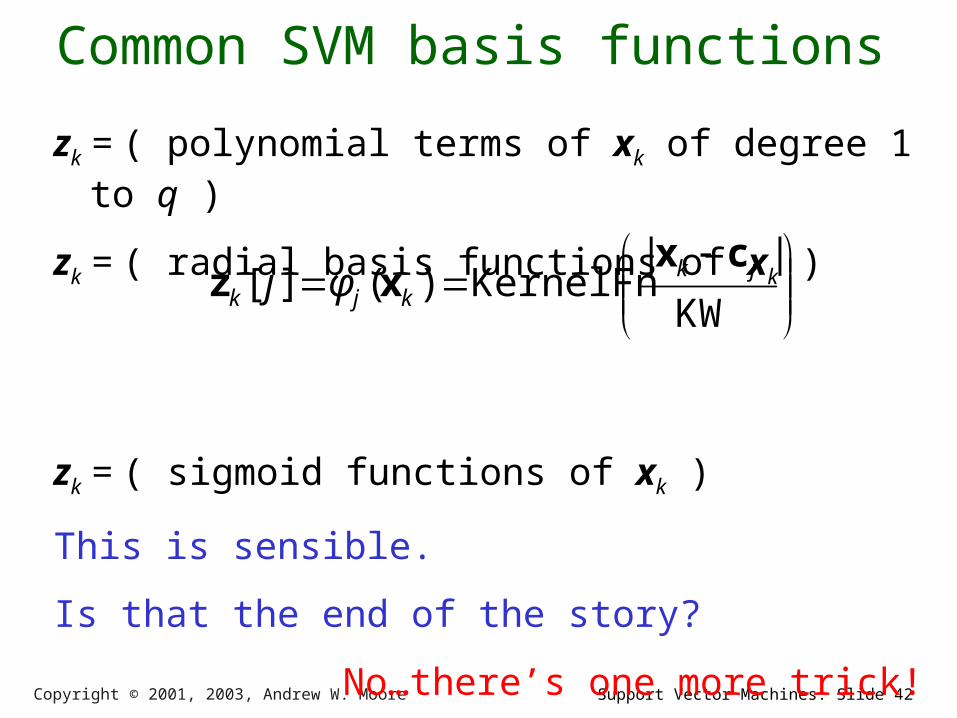
Common SVM basis functions
zk = ( polynomial terms of xk of degree 1 to q )
zk = ( radial basis functions of xk )
zk = ( sigmoid functions of xk )
This is sensible.
Is that the end of the story?
No…there’s one more trick!
KW
||KernelFn)(][ jk
kjk φjcx
xz
Support Vector Machines: Slide 43Copyright © 2001, 2003, Andrew W. Moore
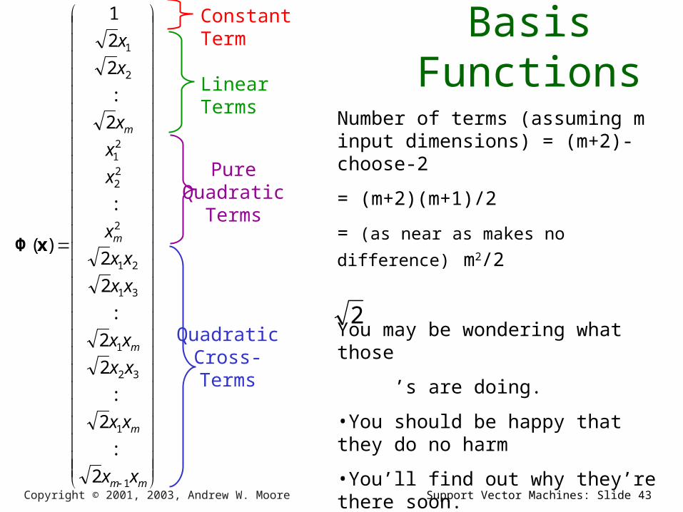
Quadratic Basis
Functions
mm
m
m
m
m
xx
xx
xx
xx
xx
xx
x
x
x
x
x
x
1
1
32
1
31
21
2
22
21
2
1
2
:
2
:
2
2
:
2
2
:
2
:
2
2
1
)(xΦ
Constant Term
Linear Terms
Pure Quadratic
Terms
Quadratic Cross-Terms
Number of terms (assuming m input dimensions) = (m+2)-choose-2
= (m+2)(m+1)/2
= (as near as makes no difference) m2/2
You may be wondering what those
’s are doing.
•You should be happy that they do no harm
•You’ll find out why they’re there soon.
2

Support Vector Machines: Slide 44Copyright © 2001, 2003, Andrew W. Moore
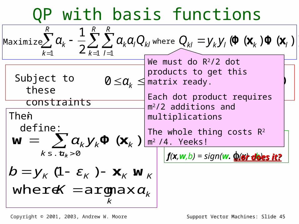
QP with basis functions
where ))().(( lklkkl yyQ xΦxΦ
Subject to these constraints:
kCαk 0
Then define:
kk
KKKK
αK
εyb
maxarg where
.)1(
wx
Then classify with:
f(x,w,b) = sign(w. (x) - b)
01
R
kkk yα
0 s.t.
)(kαk
kkk yα xΦw
Maximize
R
k
R
lkllk
R
kk Qααα
1 11 2
1
Support Vector Machines: Slide 45Copyright © 2001, 2003, Andrew W. Moore
QP with basis functionswhere ))().(( lklkkl yyQ xΦxΦ
Subject to these constraints:
kCαk 0
Then define:
kk
KKKK
αK
εyb
maxarg where
.)1(
wx
Then classify with:
f(x,w,b) = sign(w. (x) - b)
01
R
kkk yα
We must do R2/2 dot products to get this matrix ready.
Each dot product requires m2/2 additions and multiplications
The whole thing costs R2 m2 /4. Yeeks!
……or does it?or does it?
0 s.t.
)(kαk
kkk yα xΦw
Maximize
R
k
R
lkllk
R
kk Qααα
1 11 2
1
Support Vector Machines: Slide 46Copyright © 2001, 2003, Andrew W. Moore
Quadra
tic
Dot
Pro
duct
s
mm
m
m
m
m
mm
m
m
m
m
bb
bb
bb
bb
bb
bb
b
b
b
b
b
b
aa
aa
aa
aa
aa
aa
a
a
a
a
a
a
1
1
32
1
31
21
2
22
21
2
1
1
1
32
1
31
21
2
22
21
2
1
2
:
2
:
2
2
:
2
2
:
2
:
2
2
1
2
:
2
:
2
2
:
2
2
:
2
:
2
2
1
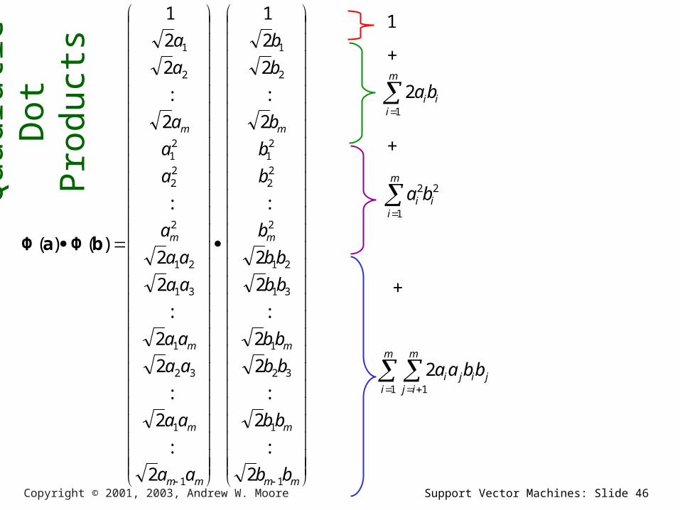
)()( bΦaΦ
1
m
iiiba
1
2
m
iii ba
1
22
m
i
m
ijjiji bbaa
1 1
2
+
+
+
Support Vector Machines: Slide 47Copyright © 2001, 2003, Andrew W. Moore
Quadra
tic
Dot
Pro
duct
s
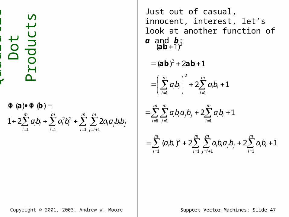
)()( bΦaΦ
m
i
m
ijjiji
m
iii
m
iii bbaababa
1 11
22
1
221
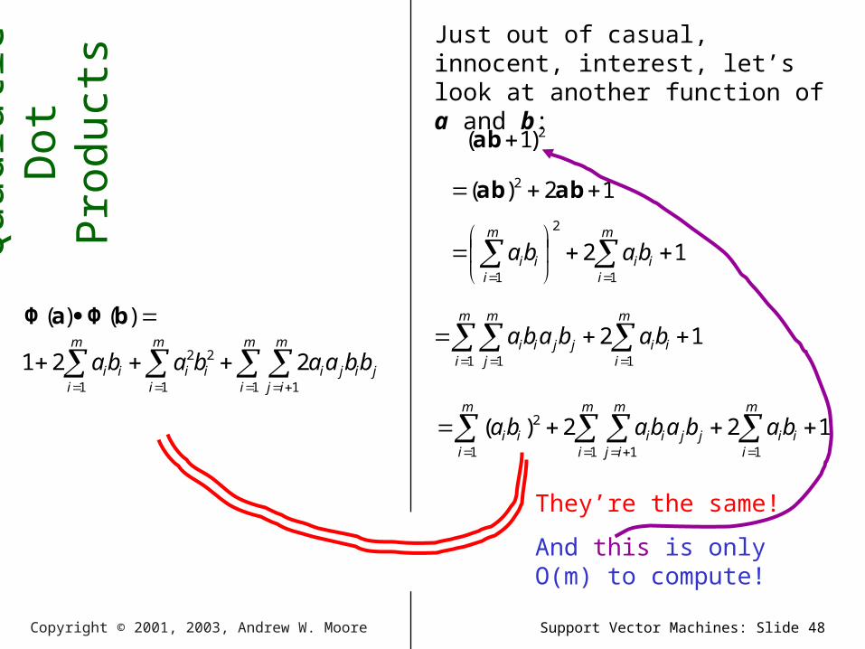
Just out of casual, innocent, interest, let’s look at another function of a and b:
2)1.( ba
1.2).( 2 baba
121
2
1
m
iii
m
iii baba
1211 1
m
iii
m
i
m
jjjii bababa
122)(11 11
2
m
iii
m
i
m
ijjjii
m
iii babababa
Support Vector Machines: Slide 48Copyright © 2001, 2003, Andrew W. Moore
Quadra
tic
Dot
Pro
duct
s
)()( bΦaΦ
Just out of casual, innocent, interest, let’s look at another function of a and b:
2)1.( ba
1.2).( 2 baba
121
2
1
m
iii
m
iii baba
1211 1
m
iii
m
i
m
jjjii bababa
122)(11 11
2
m
iii
m
i
m
ijjjii
m
iii babababa
They’re the same!
And this is only O(m) to compute!
m
i
m
ijjiji
m
iii
m
iii bbaababa
1 11
22
1
221
Support Vector Machines: Slide 49Copyright © 2001, 2003, Andrew W. Moore
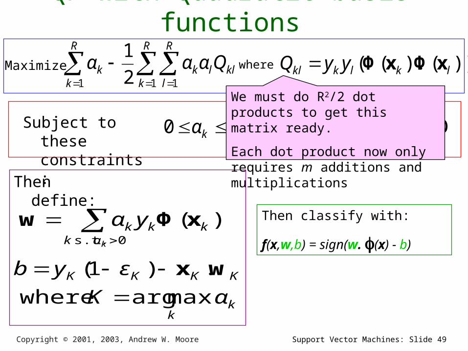
QP with Quadratic basis functions
where ))().(( lklkkl yyQ xΦxΦ
Subject to these constraints:
kCαk 0
Then define:
kk
KKKK
αK
εyb
maxarg where
.)1(
wx
Then classify with:
f(x,w,b) = sign(w. (x) - b)
01
R
kkk yα
We must do R2/2 dot products to get this matrix ready.
Each dot product now only requires m additions and multiplications
0 s.t.
)(kαk
kkk yα xΦw
Maximize
R
k
R
lkllk
R
kk Qααα
1 11 2
1

Support Vector Machines: Slide 50Copyright © 2001, 2003, Andrew W. Moore
Higher Order Polynomials
Poly-nomial
(x) Cost to build Qkl matrix traditionally
Cost if 100 inputs
(a).(b)
Cost to build Qkl matrix sneakily
Cost if 100 inputs
Quadratic
All m2/2 terms up to degree 2
m2 R2 /4 2,500 R2 (a.b+1)2
m R2 / 2 50 R2
Cubic All m3/6 terms up to degree 3
m3 R2
/1283,000 R2 (a.b+1)
3
m R2 / 2 50 R2
Quartic All m4/24 terms up to degree 4
m4 R2
/481,960,000 R2
(a.b+1)4
m R2 / 2 50 R2
Support Vector Machines: Slide 51Copyright © 2001, 2003, Andrew W. Moore
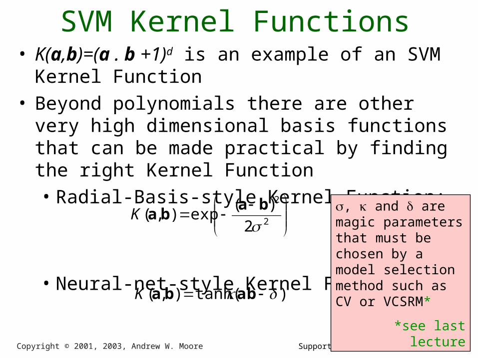
SVM Kernel Functions• K(a,b)=(a . b +1)d is an example of an SVM
Kernel Function• Beyond polynomials there are other very
high dimensional basis functions that can be made practical by finding the right Kernel Function• Radial-Basis-style Kernel Function:
• Neural-net-style Kernel Function:
2
2
2
)(exp),(
ba
baK
).tanh(),( babaK
, and are magic parameters that must be chosen by a model selection method such as CV or VCSRM*
*see last lecture
Support Vector Machines: Slide 52Copyright © 2001, 2003, Andrew W. Moore
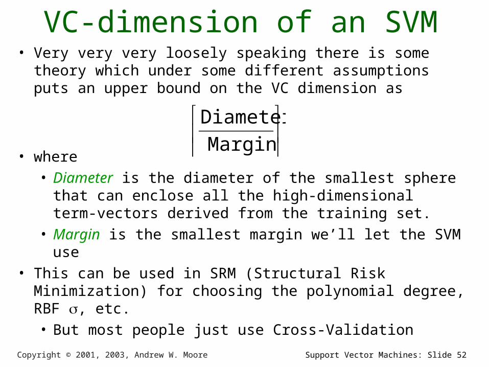
VC-dimension of an SVM• Very very very loosely speaking there is some theory
which under some different assumptions puts an upper bound on the VC dimension as
• where• Diameter is the diameter of the smallest sphere
that can enclose all the high-dimensional term-vectors derived from the training set.
• Margin is the smallest margin we’ll let the SVM use• This can be used in SRM (Structural Risk Minimization)
for choosing the polynomial degree, RBF , etc.• But most people just use Cross-Validation
Margin
Diameter
Support Vector Machines: Slide 53Copyright © 2001, 2003, Andrew W. Moore
What You Should Know• Linear SVMs• The definition of a maximum margin
classifier• What QP can do for you (but, for this class,
you don’t need to know how it does it)• How Maximum Margin can be turned into a
QP problem• How we deal with noisy (non-separable) data• How we permit non-linear boundaries• How SVM Kernel functions permit us to
pretend we’re working with ultra-high-dimensional basis-function terms
Top Related