


Languages
Pages
Legal

You can’t see this text!
Introduction to Computational Finance andFinancial EconometricsReturn Calculations
Eric ZivotWinter 2015
Eric Zivot (Copyright © 2015) Return Calculations 1 / 56
Outline
1 The time value of moneyFuture valueMultiple compounding periodsEffective annual rate
2 Asset return calculations
Eric Zivot (Copyright © 2015) Return Calculations 2 / 56

Outline
1 The time value of moneyFuture valueMultiple compounding periodsEffective annual rate
2 Asset return calculations
Eric Zivot (Copyright © 2015) Return Calculations 3 / 56

Future value
$V invested for n years at simple interest rate R per yearCompounding of interest occurs at end of year
FVn = $V · (1 + R)n ,
where FVn is future value after n years
Eric Zivot (Copyright © 2015) Return Calculations 4 / 56

Example
Consider putting $1000 in an interest checking account that pays asimple annual percentage rate of 3%. The future value after n = 1, 5and 10 years is, respectively,
FV1 = $1000 · (1.03)1 = $1030,
FV5 = $1000 · (1.03)5 = $1159.27,
FV10 = $1000 · (1.03)10 = $1343.92.
Eric Zivot (Copyright © 2015) Return Calculations 5 / 56

Future value
FV function is a relationship between four variables: FVn ,V ,R,n.Given three variables, you can solve for the fourth:
Present value:V = FVn
(1 + R)n .
Compound annual return:
R =(FVn
V
)1/n− 1.
Investment horizon:
n = ln(FVn/V )ln(1 + R) .
Eric Zivot (Copyright © 2015) Return Calculations 6 / 56
Outline
1 The time value of moneyFuture valueMultiple compounding periodsEffective annual rate
2 Asset return calculations
Eric Zivot (Copyright © 2015) Return Calculations 7 / 56

Multiple compounding periods
Compounding occurs m times per year
FV mn = $V ·
(1 + R
m
)m·n,
Rm = periodic interest rate.
Continuous compounding
FV∞n = limm→∞
$V ·(
1 + Rm
)m·n= $VeR·n ,
e1 = 2.71828.
Eric Zivot (Copyright © 2015) Return Calculations 8 / 56
Example
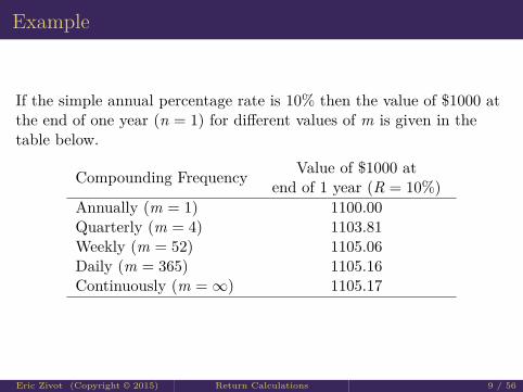
If the simple annual percentage rate is 10% then the value of $1000 atthe end of one year (n = 1) for different values of m is given in thetable below.
Compounding Frequency Value of $1000 atend of 1 year (R = 10%)
Annually (m = 1) 1100.00Quarterly (m = 4) 1103.81Weekly (m = 52) 1105.06Daily (m = 365) 1105.16Continuously (m =∞) 1105.17
Eric Zivot (Copyright © 2015) Return Calculations 9 / 56

Outline
1 The time value of moneyFuture valueMultiple compounding periodsEffective annual rate
2 Asset return calculations
Eric Zivot (Copyright © 2015) Return Calculations 10 / 56

Effective annual rate
Annual rate RA that equates FV mn with FVn ; i.e.,
$V(
1 + Rm
)m·n= $V (1 + RA)n .
Solving for RA(1 + R
m
)m= 1 + RA ⇒ RA =
(1 + R
m
)m− 1.
Eric Zivot (Copyright © 2015) Return Calculations 11 / 56

Continuous compounding
$VeR·n = $V (1 + RA)n
⇒ eR = (1 + RA)
⇒ RA = eR − 1.
Eric Zivot (Copyright © 2015) Return Calculations 12 / 56

Example
Compute effective annual rate with semi-annual compounding
The effective annual rate associated with an investment with a simpleannual rate R = 10% and semi-annual compounding (m = 2) isdetermined by solving
(1 + RA) =(
1 + 0.102
)2
⇒ RA =(
1 + 0.102
)2− 1 = 0.1025.
Eric Zivot (Copyright © 2015) Return Calculations 13 / 56

Effective annual rate
Compounding Frequency Value of $1000 atend of 1 year (R = 10%) RA
Annually (m = 1) 1100.00 10%Quarterly (m = 4) 1103.81 10.38%Weekly (m = 52) 1105.06 10.51%Daily (m = 365) 1105.16 10.52%Continuously (m =∞) 1105.17 10.52%
Eric Zivot (Copyright © 2015) Return Calculations 14 / 56

Outline
1 The time value of money
2 Asset return calculationsSimple returnsContinuously compounded (cc) returns
Eric Zivot (Copyright © 2015) Return Calculations 15 / 56

Outline
1 The time value of money
2 Asset return calculationsSimple returns
Multi-period returnsPortfolio returnsAdjusting for dividendsAdjusting for inflationAnnualizing returnsAverage returns
Continuously compounded (cc) returns
Eric Zivot (Copyright © 2015) Return Calculations 16 / 56

Simple returns
Pt = price at the end of month t on an asset that pays nodividendsPt−1 = price at the end of month t − 1
Rt = Pt − Pt−1Pt−1
= %∆Pt = net return over month t,
1 + Rt = PtPt−1
= gross return over month t.
Eric Zivot (Copyright © 2015) Return Calculations 17 / 56
Example
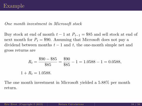
One month investment in Microsoft stock
Buy stock at end of month t − 1 at Pt−1 = $85 and sell stock at end ofnext month for Pt = $90. Assuming that Microsoft does not pay adividend between months t − 1 and t, the one-month simple net andgross returns are
Rt = $90− $85$85 = $90
$85 − 1 = 1.0588− 1 = 0.0588,
1 + Rt = 1.0588.
The one month investment in Microsoft yielded a 5.88% per monthreturn.
Eric Zivot (Copyright © 2015) Return Calculations 18 / 56

Multi-period returns
Simple two-month return
Rt(2) = Pt − Pt−2Pt−2
= PtPt−2
− 1.
Relationship to one month returns
Rt(2) = PtPt−2
− 1 = PtPt−1
· Pt−1Pt−2
− 1
= (1 + Rt) · (1 + Rt−1)− 1.
Eric Zivot (Copyright © 2015) Return Calculations 19 / 56
Multi-period returns
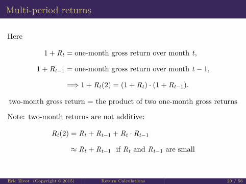
Here
1 + Rt = one-month gross return over month t,
1 + Rt−1 = one-month gross return over month t − 1,
=⇒ 1 + Rt(2) = (1 + Rt) · (1 + Rt−1).
two-month gross return = the product of two one-month gross returns
Note: two-month returns are not additive:
Rt(2) = Rt + Rt−1 + Rt · Rt−1
≈ Rt + Rt−1 if Rt and Rt−1 are small
Eric Zivot (Copyright © 2015) Return Calculations 20 / 56
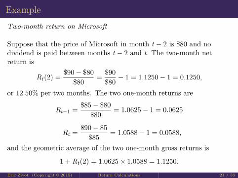
ExampleTwo-month return on Microsoft
Suppose that the price of Microsoft in month t − 2 is $80 and nodividend is paid between months t − 2 and t. The two-month netreturn is
Rt(2) = $90− $80$80 = $90
$80 − 1 = 1.1250− 1 = 0.1250,
or 12.50% per two months. The two one-month returns are
Rt−1 = $85− $80$80 = 1.0625− 1 = 0.0625
Rt = $90− 85$85 = 1.0588− 1 = 0.0588,
and the geometric average of the two one-month gross returns is
1 + Rt(2) = 1.0625× 1.0588 = 1.1250.
Eric Zivot (Copyright © 2015) Return Calculations 21 / 56

Multi-period returns
Simple k-month Return
Rt(k) = Pt − Pt−kPt−k
= PtPt−k
− 1
1 + Rt(k) = (1 + Rt) · (1 + Rt−1) · · · · · (1 + Rt−k+1)
=k−1∏j=0
(1 + Rt−j)
Note
Rt(k) 6=k−1∑j=0
Rt−j
Eric Zivot (Copyright © 2015) Return Calculations 22 / 56
Portfolio returns
Invest $V in two assets: A and B for 1 periodxA = share of $V invested in A; $V × xA = $ amountxB = share of $V invested in B; $V × xB = $ amountAssume xA + xB = 1Portfolio is defined by investment shares xA and xB
Eric Zivot (Copyright © 2015) Return Calculations 23 / 56

Portfolio returns
At the end of the period, the investments in A and B grow to
$V (1 + Rp,t) = $V [xA(1 + RA,t) + xB(1 + RB,t)]
= $V [xA + xB + xARA,t + xBRB,t ]
= $V [1 + xARA,t + xBRB,t ]
⇒ Rp,t = xARA,t + xBRB,t
The simple portfolio return is a share weighted average of the simplereturns on the individual assets.
Eric Zivot (Copyright © 2015) Return Calculations 24 / 56
Example
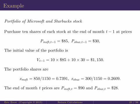
Portfolio of Microsoft and Starbucks stock
Purchase ten shares of each stock at the end of month t − 1 at prices
Pmsft,t−1 = $85, Psbux,t−1 = $30,
The initial value of the portfolio is
Vt−1 = 10× $85 + 10× 30 = $1, 150.
The portfolio shares are
xmsft = 850/1150 = 0.7391, xsbux = 300/1150 = 0.2609.
The end of month t prices are Pmsft,t = $90 and Psbux,t = $28.
Eric Zivot (Copyright © 2015) Return Calculations 25 / 56

Example cont.
Assuming Microsoft and Starbucks do not pay a dividend betweenperiods t − 1 and t, the one-period returns are
Rmsft,t = $90− $85$85 = 0.0588
Rsbux,t = $28− $30$30 = −0.0667
The return on the portfolio is
Rp,t = (0.7391)(0.0588) + (0.2609)(−0.0667) = 0.02609
and the value at the end of month t is
Vt = $1, 150× (1.02609) = $1, 180
Eric Zivot (Copyright © 2015) Return Calculations 26 / 56

Portfolio returns
In general, for a portfolio of n assets with investment shares xi suchthat x1 + · · ·+ xn = 1
1 + Rp,t =n∑
i=1xi(1 + Ri,t)
Rp,t =n∑
i=1xiRi,t
= x1R1t + · · ·+ xnRnt
Eric Zivot (Copyright © 2015) Return Calculations 27 / 56

Adjusting for dividends
Dt = dividend payment between months t − 1 and t
Rtotalt = Pt + Dt − Pt−1
Pt−1= Pt − Pt−1
Pt−1+ Dt
Pt−1
= capital gain return + dividend yield (gross)
1 + Rtotalt = Pt + Dt
Pt−1
Eric Zivot (Copyright © 2015) Return Calculations 28 / 56

Example
Total return on Microsoft stock
Buy stock in month t − 1 at Pt−1 = $85 and sell the stock the nextmonth for Pt = $90. Assume Microsoft pays a $1 dividend betweenmonths t − 1 and t. The capital gain, dividend yield and total returnare then
Rtotalt = $90 + $1− $85
$85 = $90− $85$85 + $1
$85
= 0.0588 + 0.0118
= 0.0707
The one-month investment in Microsoft yields a 7.07% per month totalreturn. The capital gain component is 5.88%, and the dividend yieldcomponent is 1.18%.
Eric Zivot (Copyright © 2015) Return Calculations 29 / 56

Adjusting for inflation
The computation of real returns on an asset is a two step process:Deflate the nominal price Pt of the asset by an index of thegeneral price level CPIt
Compute returns in the usual way using the deflated prices
PRealt = Pt
CPIt
RRealt = PReal
t − PRealt−1
PRealt−1
=Pt
CPIt− Pt−1
CPIt−1Pt−1
CPIt−1
= PtPt−1
· CPIt−1CPIt
− 1
Eric Zivot (Copyright © 2015) Return Calculations 30 / 56
Adjusting for inflation cont.
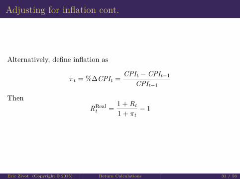
Alternatively, define inflation as
πt = %∆CPIt = CPIt − CPIt−1CPIt−1
ThenRReal
t = 1 + Rt1 + πt
− 1
Eric Zivot (Copyright © 2015) Return Calculations 31 / 56

Example
Compute real return on Microsoft stock
Suppose the CPI in months t − 1 and t is 1 and 1.01, respectively,representing a 1% monthly growth rate in the overall price level. Thereal prices of Microsoft stock are
PRealt−1 = $85
1 = $85, PRealt = $90
1.01 = $89.1089
The real monthly return is
RRealt = $89.10891− $85
$85 = 0.0483
Eric Zivot (Copyright © 2015) Return Calculations 32 / 56

Example cont.
The nominal return and inflation over the month are
Rt = $90− $85$85 = 0.0588, πt = 1.01− 1
1 = 0.01
Then the real return is
RRealt = 1.0588
1.01 − 1 = 0.0483
Notice that simple real return is almost, but not quite, equal to thesimple nominal return minus the inflation rate
RRealt ≈ Rt − πt = 0.0588− 0.01 = 0.0488
Eric Zivot (Copyright © 2015) Return Calculations 33 / 56
Annualizing returns
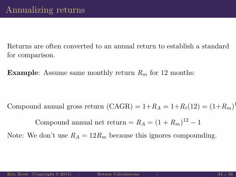
Returns are often converted to an annual return to establish a standardfor comparison.
Example: Assume same monthly return Rm for 12 months:
Compound annual gross return (CAGR) = 1+RA = 1+Rt(12) = (1+Rm)12
Compound annual net return = RA = (1 + Rm)12 − 1
Note: We don’t use RA = 12Rm because this ignores compounding.
Eric Zivot (Copyright © 2015) Return Calculations 34 / 56

Example
Annualized return on Microsoft
Suppose the one-month return, Rt , on Microsoft stock is 5.88%. If weassume that we can get this return for 12 months then thecompounded annualized return is
RA = (1.0588)12 − 1 = 1.9850− 1 = 0.9850
or 98.50% per year. Pretty good!
Eric Zivot (Copyright © 2015) Return Calculations 35 / 56

Example
Annualized return on Microsoft
Suppose the one-month return, Rt , on Microsoft stock is 5.88%. If weassume that we can get this return for 12 months then thecompounded annualized return is
RA = (1.0588)12 − 1 = 1.9850− 1 = 0.9850
or 98.50% per year. Pretty good!
Eric Zivot (Copyright © 2015) Return Calculations 36 / 56
Average returns
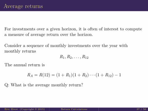
For investments over a given horizon, it is often of interest to computea measure of average return over the horizon.
Consider a sequence of monthly investments over the year withmonthly returns
R1,R2, . . . ,R12
The annual return is
RA = R(12) = (1 + R1)(1 + R2) · · · (1 + R12)− 1
Q: What is the average monthly return?
Eric Zivot (Copyright © 2015) Return Calculations 37 / 56

Average returns
Two possibilites:1 Arithmetic average (can be misleading)
R̄ = 112(R1 + · · ·+ R12)
2 Geometric average (better measure of average return)
(1 + R̄)12 = (1 + RA) = (1 + R1)(1 + R2) · · · (1 + R12)
⇒ R̄ = (1 + RA)1/12 − 1
= [(1 + R1)(1 + R2) · · · (1 + R12)]1/12 − 1
Eric Zivot (Copyright © 2015) Return Calculations 38 / 56
Example
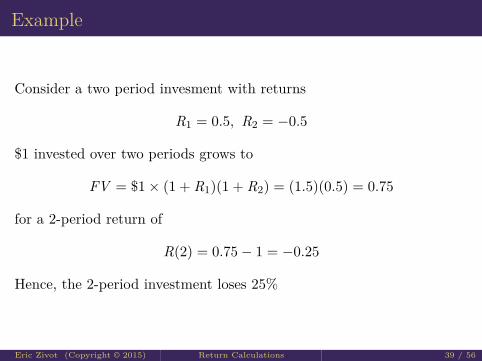
Consider a two period invesment with returns
R1 = 0.5, R2 = −0.5
$1 invested over two periods grows to
FV = $1× (1 + R1)(1 + R2) = (1.5)(0.5) = 0.75
for a 2-period return of
R(2) = 0.75− 1 = −0.25
Hence, the 2-period investment loses 25%
Eric Zivot (Copyright © 2015) Return Calculations 39 / 56

Example cont.The arithmetic average return is
R̄ = 12(0.5 +−0.5) = 0
This is misleading becuase the actual invesment lost money over the 2period horizon. The compound 2-period return based on the arithmeticaverage is
(1 + R̄)2 − 1 = 12 − 1 = 0
The geometric average is
[(1.5)(0.5)]1/2 − 1 = (0.75)1/2 − 1 = −0.1340
This is a better measure because it indicates that the investmenteventually lost money. The compound 2-period return is
(1 + R̄)2 − 1 = (0.867)2 − 1 = −0.25
Eric Zivot (Copyright © 2015) Return Calculations 40 / 56

Outline
1 The time value of money
2 Asset return calculationsSimple returnsContinuously compounded (cc) returns
Multi-period returnsPortfolio returnsAdjusting for inflation
Eric Zivot (Copyright © 2015) Return Calculations 41 / 56

Continuously compounded (cc) returns
rt = ln(1 + Rt) = ln( Pt
Pt−1
)ln(·) = natural log function
Note:
ln(1 + Rt) = rt : given Rt we can solve for rt
Rt = ert − 1 : given rt we can solve for Rt
rt is always smaller than Rt
Eric Zivot (Copyright © 2015) Return Calculations 42 / 56
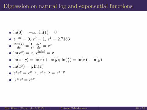
Digression on natural log and exponential functions
ln(0) = −∞, ln(1) = 0e−∞ = 0, e0 = 1, e1 = 2.7183d ln(x)
dx = 1x ,
dex
dx = ex
ln(ex) = x, eln(x) = xln(x · y) = ln(x) + ln(y); ln( x
y ) = ln(x)− ln(y)ln(xy) = y ln(x)exey = ex+y, exe−y = ex−y
(ex)y = exy
Eric Zivot (Copyright © 2015) Return Calculations 43 / 56
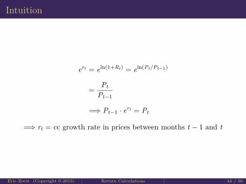
Intuition
ert = eln(1+Rt) = eln(Pt/Pt−1)
= PtPt−1
=⇒ Pt−1 · ert = Pt
=⇒ rt = cc growth rate in prices between months t − 1 and t
Eric Zivot (Copyright © 2015) Return Calculations 44 / 56
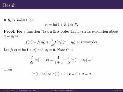
Result
If Rt is small thenrt = ln(1 + Rt) ≈ Rt
Proof. For a function f (x), a first order Taylor series expansion aboutx = x0 is
f (x) = f (x0) + ddx f (x0)(x − x0) + remainder
Let f (x) = ln(1 + x) and x0 = 0. Note that
ddx ln(1 + x) = 1
1 + x ,ddx ln(1 + x0) = 1
Thenln(1 + x) ≈ ln(1) + 1 · x = 0 + x = x
Eric Zivot (Copyright © 2015) Return Calculations 45 / 56
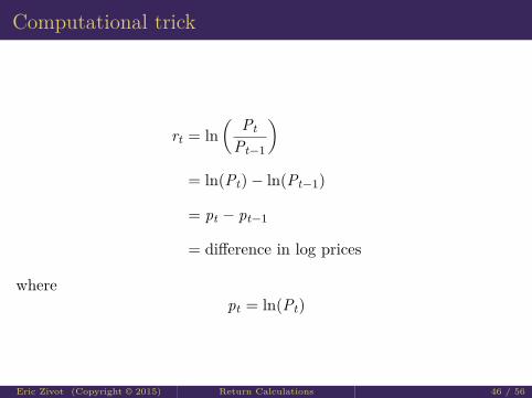
Computational trick
rt = ln( Pt
Pt−1
)= ln(Pt)− ln(Pt−1)
= pt − pt−1
= difference in log prices
wherept = ln(Pt)
Eric Zivot (Copyright © 2015) Return Calculations 46 / 56

Example
Let Pt−1 = 85,Pt = 90 and Rt = 0.0588. Then the cc monthly returncan be computed in two ways:
rt = ln(1.0588) = 0.0571
rt = ln(90)− ln(85) = 4.4998− 4.4427 = 0.0571.
Notice that rt is slightly smaller than Rt .
Eric Zivot (Copyright © 2015) Return Calculations 47 / 56
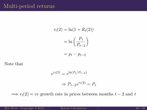
Multi-period returns
rt(2) = ln(1 + Rt(2))
= ln( Pt
Pt−2
)= pt − pt−2
Note that
ert(2) = eln(Pt/Pt−2)
⇒ Pt−2ert(2) = Pt
=⇒ rt(2) = cc growth rate in prices between months t − 2 and t
Eric Zivot (Copyright © 2015) Return Calculations 48 / 56

Result
cc returns are additive
rt(2) = ln( Pt
Pt−1· Pt−1
Pt−2
)
= ln( Pt
Pt−1
)+ ln
(Pt−1Pt−2
)= rt + rt−1
where rt = cc return between months t − 1 and t, rt−1 = cc returnbetween months t − 2 and t − 1
Eric Zivot (Copyright © 2015) Return Calculations 49 / 56
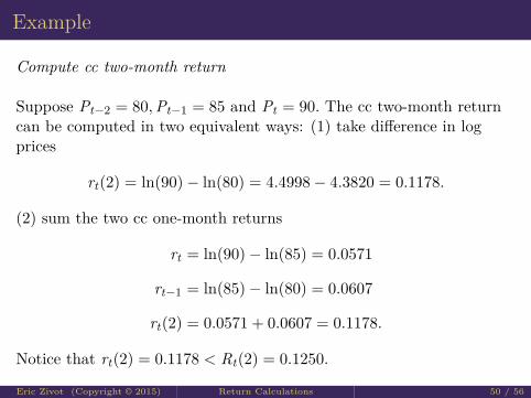
Example
Compute cc two-month return
Suppose Pt−2 = 80,Pt−1 = 85 and Pt = 90. The cc two-month returncan be computed in two equivalent ways: (1) take difference in logprices
rt(2) = ln(90)− ln(80) = 4.4998− 4.3820 = 0.1178.
(2) sum the two cc one-month returns
rt = ln(90)− ln(85) = 0.0571
rt−1 = ln(85)− ln(80) = 0.0607
rt(2) = 0.0571 + 0.0607 = 0.1178.
Notice that rt(2) = 0.1178 < Rt(2) = 0.1250.
Eric Zivot (Copyright © 2015) Return Calculations 50 / 56

Result
rt(k) = ln(1 + Rt(k)) = ln( PtPt−k
)
=k−1∑j=0
rt−j
= rt + rt−1 + · · ·+ rt−k+1
Eric Zivot (Copyright © 2015) Return Calculations 51 / 56

Portfolio returns
Rp,t =n∑
i=1xiRi,t
rp,t = ln(1 + Rp,t) = ln(1 +n∑
i=1xiRi,t) 6=
n∑i=1
xiri,t
⇒ portfolio returns are not additive
Note: If Rp,t = ∑ni=1 xiRi,t is not too large, then rp,t ≈ Rp,t otherwise,
Rp,t > rp,t .
Eric Zivot (Copyright © 2015) Return Calculations 52 / 56

ExampleCompute cc return on portfolio
Consider a portfolio of Microsoft and Starbucks stock withxmsft = 0.25, xsbux = 0.75,
Rmsft,t = 0.0588,Rsbux,t = −0.0503
Rp,t = xmsftRmsft,t + xsbux,tRsbux,t = −0.02302The cc portfolio return is
rp,t = ln(1− 0.02302) = ln(0.977) = −0.02329Note
rmsft,t = ln(1 + 0.0588) = 0.05714
rsbux,t = ln(1− 0.0503) = −0.05161
xmsftrmsft + xsbuxrsbux = −0.02442 6= rp,tEric Zivot (Copyright © 2015) Return Calculations 53 / 56

Adjusting for inflationThe cc one period real return is
rRealt = ln(1 + RReal
t )
1 + RRealt = Pt
Pt−1· CPIt−1
CPIt
It follows that
rRealt = ln
( PtPt−1
· CPIt−1CPIt
)= ln
( PtPt−1
)+ ln
(CPIt−1CPIt
)= ln(Pt)− ln(Pt−1) + ln(CPIt−1)− ln(CPIt)
= rt − πcct
wherert = ln(Pt)− ln(Pt−1) = nominal cc return
πcct = ln(CPIt)− ln(CPIt−1) = cc inflation
Eric Zivot (Copyright © 2015) Return Calculations 54 / 56
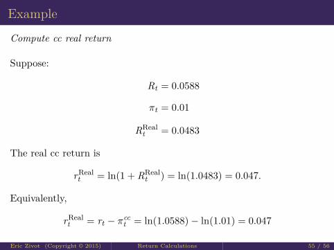
Example
Compute cc real return
Suppose:
Rt = 0.0588
πt = 0.01
RRealt = 0.0483
The real cc return is
rRealt = ln(1 + RReal
t ) = ln(1.0483) = 0.047.
Equivalently,
rRealt = rt − πcc
t = ln(1.0588)− ln(1.01) = 0.047
Eric Zivot (Copyright © 2015) Return Calculations 55 / 56

You can’t see this text!
faculty.washington.edu/ezivot/
Eric Zivot (Copyright © 2015) Return Calculations 56 / 56
Top Related