
Introduction to Computational Finance and Financial ......Title Return Calculations Author Eric...
56
You can’t see this text! Introduction to Computational Finance and Financial Econometrics Return Calculations Eric Zivot Winter 2015 Eric Zivot (Copyright © 2015) Return Calculations 1 / 56
Transcript of Introduction to Computational Finance and Financial ......Title Return Calculations Author Eric...
You can’t see this text!
Introduction to Computational Finance andFinancial EconometricsReturn Calculations
Eric ZivotWinter 2015
Eric Zivot (Copyright © 2015) Return Calculations 1 / 56
Outline
1 The time value of moneyFuture valueMultiple compounding periodsEffective annual rate
2 Asset return calculations
Eric Zivot (Copyright © 2015) Return Calculations 2 / 56

Outline
1 The time value of moneyFuture valueMultiple compounding periodsEffective annual rate
2 Asset return calculations
Eric Zivot (Copyright © 2015) Return Calculations 3 / 56

Future value
$V invested for n years at simple interest rate R per yearCompounding of interest occurs at end of year
FVn = $V · (1 + R)n ,
where FVn is future value after n years
Eric Zivot (Copyright © 2015) Return Calculations 4 / 56

Example
Consider putting $1000 in an interest checking account that pays asimple annual percentage rate of 3%. The future value after n = 1, 5and 10 years is, respectively,
FV1 = $1000 · (1.03)1 = $1030,
FV5 = $1000 · (1.03)5 = $1159.27,
FV10 = $1000 · (1.03)10 = $1343.92.
Eric Zivot (Copyright © 2015) Return Calculations 5 / 56

Future value
FV function is a relationship between four variables: FVn ,V ,R,n.Given three variables, you can solve for the fourth:
Present value:V = FVn
(1 + R)n .
Compound annual return:
R =(FVn
V
)1/n− 1.
Investment horizon:
n = ln(FVn/V )ln(1 + R) .
Eric Zivot (Copyright © 2015) Return Calculations 6 / 56
Outline
1 The time value of moneyFuture valueMultiple compounding periodsEffective annual rate
2 Asset return calculations
Eric Zivot (Copyright © 2015) Return Calculations 7 / 56

Multiple compounding periods
Compounding occurs m times per year
FV mn = $V ·
(1 + R
m
)m·n,
Rm = periodic interest rate.
Continuous compounding
FV∞n = limm→∞
$V ·(
1 + Rm
)m·n= $VeR·n ,
e1 = 2.71828.
Eric Zivot (Copyright © 2015) Return Calculations 8 / 56
Example
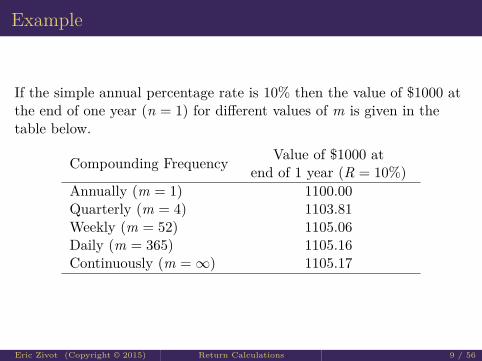
If the simple annual percentage rate is 10% then the value of $1000 atthe end of one year (n = 1) for different values of m is given in thetable below.
Compounding Frequency Value of $1000 atend of 1 year (R = 10%)
Annually (m = 1) 1100.00Quarterly (m = 4) 1103.81Weekly (m = 52) 1105.06Daily (m = 365) 1105.16Continuously (m =∞) 1105.17
Eric Zivot (Copyright © 2015) Return Calculations 9 / 56

Outline
1 The time value of moneyFuture valueMultiple compounding periodsEffective annual rate
2 Asset return calculations
Eric Zivot (Copyright © 2015) Return Calculations 10 / 56

Effective annual rate
Annual rate RA that equates FV mn with FVn ; i.e.,
$V(
1 + Rm
)m·n= $V (1 + RA)n .
Solving for RA(1 + R
m
)m= 1 + RA ⇒ RA =
(1 + R
m
)m− 1.
Eric Zivot (Copyright © 2015) Return Calculations 11 / 56

Continuous compounding
$VeR·n = $V (1 + RA)n
⇒ eR = (1 + RA)
⇒ RA = eR − 1.
Eric Zivot (Copyright © 2015) Return Calculations 12 / 56

Example
Compute effective annual rate with semi-annual compounding
The effective annual rate associated with an investment with a simpleannual rate R = 10% and semi-annual compounding (m = 2) isdetermined by solving
(1 + RA) =(
1 + 0.102
)2
⇒ RA =(
1 + 0.102
)2− 1 = 0.1025.
Eric Zivot (Copyright © 2015) Return Calculations 13 / 56

Effective annual rate
Compounding Frequency Value of $1000 atend of 1 year (R = 10%) RA
Annually (m = 1) 1100.00 10%Quarterly (m = 4) 1103.81 10.38%Weekly (m = 52) 1105.06 10.51%Daily (m = 365) 1105.16 10.52%Continuously (m =∞) 1105.17 10.52%
Eric Zivot (Copyright © 2015) Return Calculations 14 / 56

Outline
1 The time value of money
2 Asset return calculationsSimple returnsContinuously compounded (cc) returns
Eric Zivot (Copyright © 2015) Return Calculations 15 / 56

Outline
1 The time value of money
2 Asset return calculationsSimple returns
Multi-period returnsPortfolio returnsAdjusting for dividendsAdjusting for inflationAnnualizing returnsAverage returns
Continuously compounded (cc) returns
Eric Zivot (Copyright © 2015) Return Calculations 16 / 56

Simple returns
Pt = price at the end of month t on an asset that pays nodividendsPt−1 = price at the end of month t − 1
Rt = Pt − Pt−1Pt−1
= %∆Pt = net return over month t,
1 + Rt = PtPt−1
= gross return over month t.
Eric Zivot (Copyright © 2015) Return Calculations 17 / 56
Example
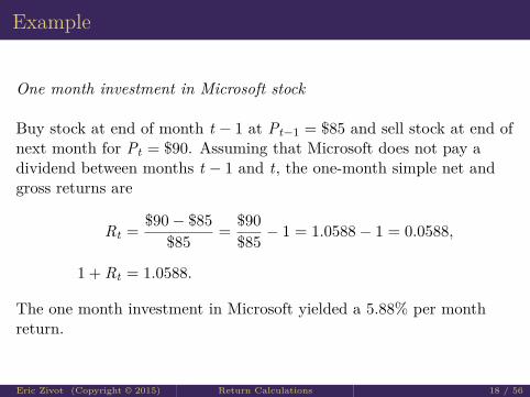
One month investment in Microsoft stock
Buy stock at end of month t − 1 at Pt−1 = $85 and sell stock at end ofnext month for Pt = $90. Assuming that Microsoft does not pay adividend between months t − 1 and t, the one-month simple net andgross returns are
Rt = $90− $85$85 = $90
$85 − 1 = 1.0588− 1 = 0.0588,
1 + Rt = 1.0588.
The one month investment in Microsoft yielded a 5.88% per monthreturn.
Eric Zivot (Copyright © 2015) Return Calculations 18 / 56

Multi-period returns
Simple two-month return
Rt(2) = Pt − Pt−2Pt−2
= PtPt−2
− 1.
Relationship to one month returns
Rt(2) = PtPt−2
− 1 = PtPt−1
· Pt−1Pt−2
− 1
= (1 + Rt) · (1 + Rt−1)− 1.
Eric Zivot (Copyright © 2015) Return Calculations 19 / 56
Multi-period returns
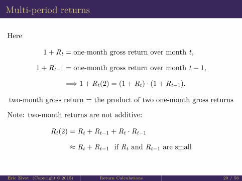
Here
1 + Rt = one-month gross return over month t,
1 + Rt−1 = one-month gross return over month t − 1,
=⇒ 1 + Rt(2) = (1 + Rt) · (1 + Rt−1).
two-month gross return = the product of two one-month gross returns
Note: two-month returns are not additive:
Rt(2) = Rt + Rt−1 + Rt · Rt−1
≈ Rt + Rt−1 if Rt and Rt−1 are small
Eric Zivot (Copyright © 2015) Return Calculations 20 / 56
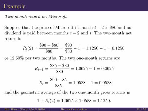
ExampleTwo-month return on Microsoft
Suppose that the price of Microsoft in month t − 2 is $80 and nodividend is paid between months t − 2 and t. The two-month netreturn is
Rt(2) = $90− $80$80 = $90
$80 − 1 = 1.1250− 1 = 0.1250,
or 12.50% per two months. The two one-month returns are
Rt−1 = $85− $80$80 = 1.0625− 1 = 0.0625
Rt = $90− 85$85 = 1.0588− 1 = 0.0588,
and the geometric average of the two one-month gross returns is
1 + Rt(2) = 1.0625× 1.0588 = 1.1250.
Eric Zivot (Copyright © 2015) Return Calculations 21 / 56

Multi-period returns
Simple k-month Return
Rt(k) = Pt − Pt−kPt−k
= PtPt−k
− 1
1 + Rt(k) = (1 + Rt) · (1 + Rt−1) · · · · · (1 + Rt−k+1)
=k−1∏j=0
(1 + Rt−j)
Note
Rt(k) 6=k−1∑j=0
Rt−j
Eric Zivot (Copyright © 2015) Return Calculations 22 / 56
Portfolio returns
Invest $V in two assets: A and B for 1 periodxA = share of $V invested in A; $V × xA = $ amountxB = share of $V invested in B; $V × xB = $ amountAssume xA + xB = 1Portfolio is defined by investment shares xA and xB
Eric Zivot (Copyright © 2015) Return Calculations 23 / 56

Portfolio returns
At the end of the period, the investments in A and B grow to
$V (1 + Rp,t) = $V [xA(1 + RA,t) + xB(1 + RB,t)]
= $V [xA + xB + xARA,t + xBRB,t ]
= $V [1 + xARA,t + xBRB,t ]
⇒ Rp,t = xARA,t + xBRB,t
The simple portfolio return is a share weighted average of the simplereturns on the individual assets.
Eric Zivot (Copyright © 2015) Return Calculations 24 / 56
Example
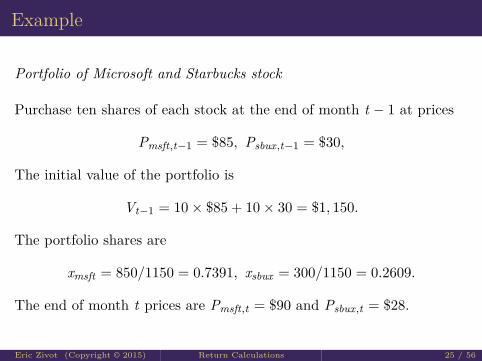
Portfolio of Microsoft and Starbucks stock
Purchase ten shares of each stock at the end of month t − 1 at prices
Pmsft,t−1 = $85, Psbux,t−1 = $30,
The initial value of the portfolio is
Vt−1 = 10× $85 + 10× 30 = $1, 150.
The portfolio shares are
xmsft = 850/1150 = 0.7391, xsbux = 300/1150 = 0.2609.
The end of month t prices are Pmsft,t = $90 and Psbux,t = $28.
Eric Zivot (Copyright © 2015) Return Calculations 25 / 56

Example cont.
Assuming Microsoft and Starbucks do not pay a dividend betweenperiods t − 1 and t, the one-period returns are
Rmsft,t = $90− $85$85 = 0.0588
Rsbux,t = $28− $30$30 = −0.0667
The return on the portfolio is
Rp,t = (0.7391)(0.0588) + (0.2609)(−0.0667) = 0.02609
and the value at the end of month t is
Vt = $1, 150× (1.02609) = $1, 180
Eric Zivot (Copyright © 2015) Return Calculations 26 / 56

Portfolio returns
In general, for a portfolio of n assets with investment shares xi suchthat x1 + · · ·+ xn = 1
1 + Rp,t =n∑
i=1xi(1 + Ri,t)
Rp,t =n∑
i=1xiRi,t
= x1R1t + · · ·+ xnRnt
Eric Zivot (Copyright © 2015) Return Calculations 27 / 56

Adjusting for dividends
Dt = dividend payment between months t − 1 and t
Rtotalt = Pt + Dt − Pt−1
Pt−1= Pt − Pt−1
Pt−1+ Dt
Pt−1
= capital gain return + dividend yield (gross)
1 + Rtotalt = Pt + Dt
Pt−1
Eric Zivot (Copyright © 2015) Return Calculations 28 / 56

Example
Total return on Microsoft stock
Buy stock in month t − 1 at Pt−1 = $85 and sell the stock the nextmonth for Pt = $90. Assume Microsoft pays a $1 dividend betweenmonths t − 1 and t. The capital gain, dividend yield and total returnare then
Rtotalt = $90 + $1− $85
$85 = $90− $85$85 + $1
$85
= 0.0588 + 0.0118
= 0.0707
The one-month investment in Microsoft yields a 7.07% per month totalreturn. The capital gain component is 5.88%, and the dividend yieldcomponent is 1.18%.
Eric Zivot (Copyright © 2015) Return Calculations 29 / 56

Adjusting for inflation
The computation of real returns on an asset is a two step process:Deflate the nominal price Pt of the asset by an index of thegeneral price level CPIt
Compute returns in the usual way using the deflated prices
PRealt = Pt
CPIt
RRealt = PReal
t − PRealt−1
PRealt−1
=Pt
CPIt− Pt−1
CPIt−1Pt−1
CPIt−1
= PtPt−1
· CPIt−1CPIt
− 1
Eric Zivot (Copyright © 2015) Return Calculations 30 / 56
Adjusting for inflation cont.
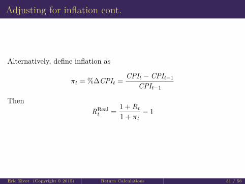
Alternatively, define inflation as
πt = %∆CPIt = CPIt − CPIt−1CPIt−1
ThenRReal
t = 1 + Rt1 + πt
− 1
Eric Zivot (Copyright © 2015) Return Calculations 31 / 56

Example
Compute real return on Microsoft stock
Suppose the CPI in months t − 1 and t is 1 and 1.01, respectively,representing a 1% monthly growth rate in the overall price level. Thereal prices of Microsoft stock are
PRealt−1 = $85
1 = $85, PRealt = $90
1.01 = $89.1089
The real monthly return is
RRealt = $89.10891− $85
$85 = 0.0483
Eric Zivot (Copyright © 2015) Return Calculations 32 / 56

Example cont.
The nominal return and inflation over the month are
Rt = $90− $85$85 = 0.0588, πt = 1.01− 1
1 = 0.01
Then the real return is
RRealt = 1.0588
1.01 − 1 = 0.0483
Notice that simple real return is almost, but not quite, equal to thesimple nominal return minus the inflation rate
RRealt ≈ Rt − πt = 0.0588− 0.01 = 0.0488
Eric Zivot (Copyright © 2015) Return Calculations 33 / 56
Annualizing returns
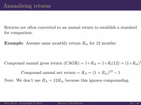
Returns are often converted to an annual return to establish a standardfor comparison.
Example: Assume same monthly return Rm for 12 months:
Compound annual gross return (CAGR) = 1+RA = 1+Rt(12) = (1+Rm)12
Compound annual net return = RA = (1 + Rm)12 − 1
Note: We don’t use RA = 12Rm because this ignores compounding.
Eric Zivot (Copyright © 2015) Return Calculations 34 / 56

Example
Annualized return on Microsoft
Suppose the one-month return, Rt , on Microsoft stock is 5.88%. If weassume that we can get this return for 12 months then thecompounded annualized return is
RA = (1.0588)12 − 1 = 1.9850− 1 = 0.9850
or 98.50% per year. Pretty good!
Eric Zivot (Copyright © 2015) Return Calculations 35 / 56

Example
Annualized return on Microsoft
Suppose the one-month return, Rt , on Microsoft stock is 5.88%. If weassume that we can get this return for 12 months then thecompounded annualized return is
RA = (1.0588)12 − 1 = 1.9850− 1 = 0.9850
or 98.50% per year. Pretty good!
Eric Zivot (Copyright © 2015) Return Calculations 36 / 56
Average returns
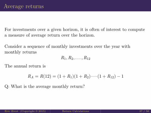
For investments over a given horizon, it is often of interest to computea measure of average return over the horizon.
Consider a sequence of monthly investments over the year withmonthly returns
R1,R2, . . . ,R12
The annual return is
RA = R(12) = (1 + R1)(1 + R2) · · · (1 + R12)− 1
Q: What is the average monthly return?
Eric Zivot (Copyright © 2015) Return Calculations 37 / 56

Average returns
Two possibilites:1 Arithmetic average (can be misleading)
R̄ = 112(R1 + · · ·+ R12)
2 Geometric average (better measure of average return)
(1 + R̄)12 = (1 + RA) = (1 + R1)(1 + R2) · · · (1 + R12)
⇒ R̄ = (1 + RA)1/12 − 1
= [(1 + R1)(1 + R2) · · · (1 + R12)]1/12 − 1
Eric Zivot (Copyright © 2015) Return Calculations 38 / 56
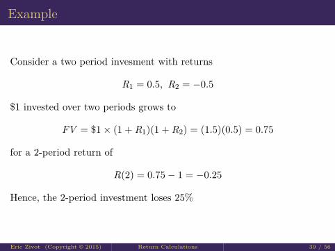
Example
Consider a two period invesment with returns
R1 = 0.5, R2 = −0.5
$1 invested over two periods grows to
FV = $1× (1 + R1)(1 + R2) = (1.5)(0.5) = 0.75
for a 2-period return of
R(2) = 0.75− 1 = −0.25
Hence, the 2-period investment loses 25%
Eric Zivot (Copyright © 2015) Return Calculations 39 / 56

Example cont.The arithmetic average return is
R̄ = 12(0.5 +−0.5) = 0
This is misleading becuase the actual invesment lost money over the 2period horizon. The compound 2-period return based on the arithmeticaverage is
(1 + R̄)2 − 1 = 12 − 1 = 0
The geometric average is
[(1.5)(0.5)]1/2 − 1 = (0.75)1/2 − 1 = −0.1340
This is a better measure because it indicates that the investmenteventually lost money. The compound 2-period return is
(1 + R̄)2 − 1 = (0.867)2 − 1 = −0.25
Eric Zivot (Copyright © 2015) Return Calculations 40 / 56

Outline
1 The time value of money
2 Asset return calculationsSimple returnsContinuously compounded (cc) returns
Multi-period returnsPortfolio returnsAdjusting for inflation
Eric Zivot (Copyright © 2015) Return Calculations 41 / 56

Continuously compounded (cc) returns
rt = ln(1 + Rt) = ln( Pt
Pt−1
)ln(·) = natural log function
Note:
ln(1 + Rt) = rt : given Rt we can solve for rt
Rt = ert − 1 : given rt we can solve for Rt
rt is always smaller than Rt
Eric Zivot (Copyright © 2015) Return Calculations 42 / 56
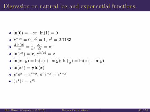
Digression on natural log and exponential functions
ln(0) = −∞, ln(1) = 0e−∞ = 0, e0 = 1, e1 = 2.7183d ln(x)
dx = 1x ,
dex
dx = ex
ln(ex) = x, eln(x) = xln(x · y) = ln(x) + ln(y); ln( x
y ) = ln(x)− ln(y)ln(xy) = y ln(x)exey = ex+y, exe−y = ex−y
(ex)y = exy
Eric Zivot (Copyright © 2015) Return Calculations 43 / 56
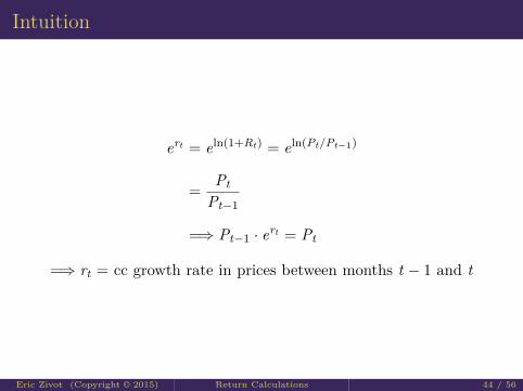
Intuition
ert = eln(1+Rt) = eln(Pt/Pt−1)
= PtPt−1
=⇒ Pt−1 · ert = Pt
=⇒ rt = cc growth rate in prices between months t − 1 and t
Eric Zivot (Copyright © 2015) Return Calculations 44 / 56
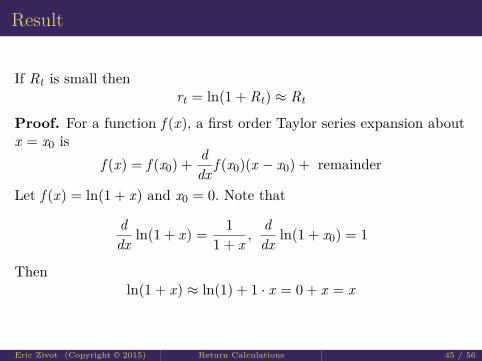
Result
If Rt is small thenrt = ln(1 + Rt) ≈ Rt
Proof. For a function f (x), a first order Taylor series expansion aboutx = x0 is
f (x) = f (x0) + ddx f (x0)(x − x0) + remainder
Let f (x) = ln(1 + x) and x0 = 0. Note that
ddx ln(1 + x) = 1
1 + x ,ddx ln(1 + x0) = 1
Thenln(1 + x) ≈ ln(1) + 1 · x = 0 + x = x
Eric Zivot (Copyright © 2015) Return Calculations 45 / 56
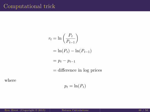
Computational trick
rt = ln( Pt
Pt−1
)= ln(Pt)− ln(Pt−1)
= pt − pt−1
= difference in log prices
wherept = ln(Pt)
Eric Zivot (Copyright © 2015) Return Calculations 46 / 56

Example
Let Pt−1 = 85,Pt = 90 and Rt = 0.0588. Then the cc monthly returncan be computed in two ways:
rt = ln(1.0588) = 0.0571
rt = ln(90)− ln(85) = 4.4998− 4.4427 = 0.0571.
Notice that rt is slightly smaller than Rt .
Eric Zivot (Copyright © 2015) Return Calculations 47 / 56
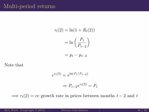
Multi-period returns
rt(2) = ln(1 + Rt(2))
= ln( Pt
Pt−2
)= pt − pt−2
Note that
ert(2) = eln(Pt/Pt−2)
⇒ Pt−2ert(2) = Pt
=⇒ rt(2) = cc growth rate in prices between months t − 2 and t
Eric Zivot (Copyright © 2015) Return Calculations 48 / 56

Result
cc returns are additive
rt(2) = ln( Pt
Pt−1· Pt−1
Pt−2
)
= ln( Pt
Pt−1
)+ ln
(Pt−1Pt−2
)= rt + rt−1
where rt = cc return between months t − 1 and t, rt−1 = cc returnbetween months t − 2 and t − 1
Eric Zivot (Copyright © 2015) Return Calculations 49 / 56
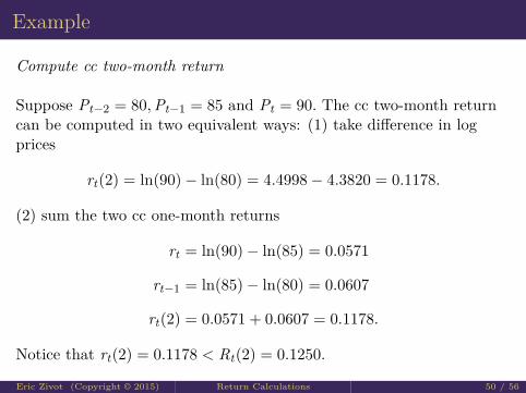
Example
Compute cc two-month return
Suppose Pt−2 = 80,Pt−1 = 85 and Pt = 90. The cc two-month returncan be computed in two equivalent ways: (1) take difference in logprices
rt(2) = ln(90)− ln(80) = 4.4998− 4.3820 = 0.1178.
(2) sum the two cc one-month returns
rt = ln(90)− ln(85) = 0.0571
rt−1 = ln(85)− ln(80) = 0.0607
rt(2) = 0.0571 + 0.0607 = 0.1178.
Notice that rt(2) = 0.1178 < Rt(2) = 0.1250.
Eric Zivot (Copyright © 2015) Return Calculations 50 / 56

Result
rt(k) = ln(1 + Rt(k)) = ln( PtPt−k
)
=k−1∑j=0
rt−j
= rt + rt−1 + · · ·+ rt−k+1
Eric Zivot (Copyright © 2015) Return Calculations 51 / 56

Portfolio returns
Rp,t =n∑
i=1xiRi,t
rp,t = ln(1 + Rp,t) = ln(1 +n∑
i=1xiRi,t) 6=
n∑i=1
xiri,t
⇒ portfolio returns are not additive
Note: If Rp,t = ∑ni=1 xiRi,t is not too large, then rp,t ≈ Rp,t otherwise,
Rp,t > rp,t .
Eric Zivot (Copyright © 2015) Return Calculations 52 / 56

ExampleCompute cc return on portfolio
Consider a portfolio of Microsoft and Starbucks stock withxmsft = 0.25, xsbux = 0.75,
Rmsft,t = 0.0588,Rsbux,t = −0.0503
Rp,t = xmsftRmsft,t + xsbux,tRsbux,t = −0.02302The cc portfolio return is
rp,t = ln(1− 0.02302) = ln(0.977) = −0.02329Note
rmsft,t = ln(1 + 0.0588) = 0.05714
rsbux,t = ln(1− 0.0503) = −0.05161
xmsftrmsft + xsbuxrsbux = −0.02442 6= rp,tEric Zivot (Copyright © 2015) Return Calculations 53 / 56

Adjusting for inflationThe cc one period real return is
rRealt = ln(1 + RReal
t )
1 + RRealt = Pt
Pt−1· CPIt−1
CPIt
It follows that
rRealt = ln
( PtPt−1
· CPIt−1CPIt
)= ln
( PtPt−1
)+ ln
(CPIt−1CPIt
)= ln(Pt)− ln(Pt−1) + ln(CPIt−1)− ln(CPIt)
= rt − πcct
wherert = ln(Pt)− ln(Pt−1) = nominal cc return
πcct = ln(CPIt)− ln(CPIt−1) = cc inflation
Eric Zivot (Copyright © 2015) Return Calculations 54 / 56
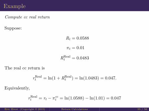
Example
Compute cc real return
Suppose:
Rt = 0.0588
πt = 0.01
RRealt = 0.0483
The real cc return is
rRealt = ln(1 + RReal
t ) = ln(1.0483) = 0.047.
Equivalently,
rRealt = rt − πcc
t = ln(1.0588)− ln(1.01) = 0.047
Eric Zivot (Copyright © 2015) Return Calculations 55 / 56

You can’t see this text!
faculty.washington.edu/ezivot/
Eric Zivot (Copyright © 2015) Return Calculations 56 / 56


![A computational interface for thermodynamic calculations ...en.iric.imet-db.ru/PDF/89.pdf · phase equilibria present in a system [1]. ... in incorporating thermodynamic calculations](https://static.fdocuments.us/doc/165x107/5f1fbfe8619c374f3e7ece78/a-computational-interface-for-thermodynamic-calculations-eniricimet-dbrupdf89pdf.jpg)


![Domentijan - Zivot Sv.simeona i Sv.save [Djura Danicic, 1865] Google](https://static.fdocuments.us/doc/165x107/5460caabb1af9feb588b5361/domentijan-zivot-svsimeona-i-svsave-djura-danicic-1865-google.jpg)

