


Languages
Pages
Legal


1
Integrated Design Process for the Development of
Semi-Active Landing Gears for Transport Aircraft
Bei der Fakultät für Luft- und Raumfahrttechnik der Universität Stuttgart
zur Erlangung der Würde eines Doktors der
Ingenieurwissenschaften (Dr.-Ing.) genehmigte Abhandlung
vorgelegt von
Wolf Krüger
aus Hannover
Hauptberichter: Prof. K. Well, Ph.D.
Mitberichter: Prof. Dr.-Ing. habil. D. Bestle
Tag der mündlichen Prüfung: 18.12.2000
Institut für Flugmechanik und Flugregelung der Universität Stuttgart
2000

2
Aircraft Landing Gears, Active Landing Gears, Semi-active Control, Multibody Simulation,
Roll Comfort, Multi-objective Optimization, Rough Runways
Abstract
Aircraft landing gears are currently optimized to have optimal performance in the rare case of
a hard landing. The resulting suspension layout may lead to unsatisfactory oscillations when
the aircraft is taxiing on a rough runway; runway unevenness can excite elastic structural
modes, leading to passenger and crew discomfort.
Although there are existing modifications of aircraft shock absorbers to reduce the problem,
the basic design conflict between the requirements for landing and for rolling cannot be fully
overcome by a passive suspension layout. Semi-active suspension techniques promise a solu-
tion to this problem. A semi-active suspension, i.e. a damper with a variable, controlled orifice
cross-section, is capable of reducing fuselage vibrations effectively while being relatively
light-weight and of low system complexity.
In the thesis, three control laws, a skyhook-type controller, a fuzzy-logic controller, and a state
feedback controller are designed for the application to a semi-active suspension for an aircraft
nose landing gear. Regarding the aircraft flexibility, the landing gears can no longer be
designed independently from the aircraft. The layout of the controllers is therefore undertaken
using an integrated design approach. Airframe and landing gear properties are determined tak-
ing into consideration models from different engineering disciplines involved in the aircraft
development process, making the oleo design part of the concurrent engineering loop.
The aircraft model is set up in a multibody simulation environment. The control laws are
developed in a control design tool; special consideration is given to the requirements of semi-
active actuators. The controllers are exported into the simulation environment and their param-
eters are optimized by means of multi-objective optimization. In a further step, the perfor-
mance of the three control strategies are compared with each other and additionally with
passive and fully active approaches. The dependence of the control performance on operational
parameters (aircraft weight and speed, runway roughness) is assessed, and limitations due to
realistic actuator restrictions are discussed. Finally, the benefits and disadvantages of semi-
active nose landing gear control are summarized and open problems are addressed.

3
Flugzeug-Fahrwerke, Aktive Fahrwerke, Semiaktive Regelung, Mehrkörpersimulation, Roll-
komfort, mehrzielige Optimierung, schlechte Rollbahnen
Zusammenfassung
Flugzeugfahrwerke werden zur Zeit für den seltenen Fall einer harten Landung optimiert. Die
sich daraus ergebende Stoßdämpferauslegung kann zu unerwünschten Schwingungen beim
Rollen über unebene Start- und Landebahnen führen. Durch Strukturschwingungen kann es zu
erheblichen Komforteinbußen bei Passagieren und Crew kommen.
Obwohl der Einsatz modifizierter Stoßdämpfer das Verhalten des Flugzeugs am Boden verbes-
sert, kann der zugrunde liegende Zielkonflikt zwischen der Auslegung für die Landung und
derjenigen für das Rollen durch passive Systeme nicht vollständig gelöst werden. Semi-aktive
Stoßdämpfer, die mit einem variablen, regelbaren Drosselquerschnitt arbeiten, sind dagegen in
der Lage, die Rumpfschwingungen effektiv zu verringern. Gleichzeitig stellen sie eine relativ
leichte und mechanisch unkomplizierte Alternative zu herkömmlichen Systemen dar.
In dieser Dissertation werden drei Regelgesetze, ein Skyhook-Regler, ein Fuzzy-Regler und
ein Zustandsregler, für die Anwendung auf ein semi-aktives Bugfahrwerk entworfen. Der Ent-
wurf der Fahrwerke kann heute nicht mehr unabhängig vom Entwurf des Rumpfes geschehen,
da die Strukturelastizitäten eine wichtige Rolle spielen. Daher werden die Regelgesetze mit
Methoden des Integrierten Entwurfs ausgelegt, wobei die Eigenschaften von Rumpf, Flügeln
und Fahrwerk durch die Einbindung von Modellen aus verschiedenen Fachdisziplinen berück-
sichtigt werden. Durch dieses Verfahren findet die Auslegung der Stoßdämpfer Eingang in den
„Concurrent Engineering“ - Prozess.
Das Flugzeugmodell wird als elastisches Mehrkörpermodell aufgebaut. Die Regelgesetze wer-
den in einem Programm für den Reglerentwurf ausgelegt. Beim Entwurf werden die Besonder-
heiten der semi-aktiven Regelung berücksichtigt. Die Regler werden in die
Simulationsumgebung exportiert und die endgültigen Reglerparameter durch die Strategie der
mehrzieligen Optimierung gefunden. In einem weiteren Schritt wird die Effizienz der Regler
untereinander verglichen und dem Verhalten eines passiven sowie eines voll aktiven Systems
gegenübergestellt. Des Weiteren wird die Abhängigkeit der Regelqualität von den Einsatzbe-
dingungen (Flugzeuggewicht, Geschwindigkeit), sowie die Beschränkungen, die sich durch
den Einsatz realistischer Stellglieder ergeben, untersucht. Schließlich werden die Vor- und
Nachteile der semi-aktiven Regelung diskutiert und offene Punkte angesprochen.

4

5
Acknowledgments
The work was performed in the Department for Vehicle System Dynamics of the Institute for
Aeroelasticity at the German Aerospace Center in Oberpfaffenhofen, partly under a grant of
EADS Aerospace Airbus, Hamburg.
First of all I would like to express my thanks to Prof. W. Kortüm of the German Aerospace
Center in Oberpfaffenhofen who, as a principal advisor, has strongly supported this work and
has been ready to give educational and technical advice at any time.
I would further like to thank Prof. K. Well of the University of Stuttgart who has shown a lot of
interest in this work which has much benefited from his inputs, and who has made it possible
for me to conduct the thesis at the Institute for Flight Mechanics and Flight Control in
Stuttgart.
Equally, I am indebted to Prof. D. Bestle who not only agreed to join as second reviewer on
short notice but also did a very thorough revision of the work.
The Department for Vehicle Systems Dynamics in Oberpfaffenhofen has provided a unique
working environment. My thanks go to all my colleagues who have always been open to pro-
vide assistance and information without which the work in this form would not have been pos-
sible. Knowing I will not be able here to give everybody the justice he deserves I would
nevertheless like to thank especially K. Deutrich, A. Veitl, M. Spieck, and W. Rulka.
From the industrial partners I want to thank especially Mr. R. Sonder and Mr. G. Roloff from
EADS Airbus Hamburg, as well as Mr. U. Grabherr from Liebherr Aerospace Lindenberg, for
providing realistic data and discussing the results.
Finally my thanks go to my wife and my parents for the continuous support they gave while the
thesis was taking shape.

6

7
1 Semi-Active Landing Gears for the Reduction of Ground Induced Vibrations 13
1.1 Problems of Large Transport Aircraft - Ground Induced Vibrationsand their Effects 13
1.2 Aircraft Suspension Control - The Solution? . . . . . . . . . . . . . . . . . . . . . . . . . . . . .14
1.3 An Integrated Design Process for Semi-Active Landing Gears . . . . . . . . . . . . . . .16
2 Landing Gear Development as an Integral Part of Aircraft Design 19
2.1 Aircraft Landing Gears: Requirements and Configurations. . . . . . . . . . . . . . . . . .19
2.1.1 Landing Gear Requirements . . . . . . . . . . . . . . . . . . . . . . . . . . . . . . . . .19
2.1.2 Landing Gear Configurations . . . . . . . . . . . . . . . . . . . . . . . . . . . . . . . .20
2.2 Conventional, Active, and Semi-Active Landing Gears . . . . . . . . . . . . . . . . . . . .22
2.2.1 Conventional Landing Gears . . . . . . . . . . . . . . . . . . . . . . . . . . . . . . . . .22
2.2.2 Landing Gears of Variable Characteristics . . . . . . . . . . . . . . . . . . . . . .25
2.2.3 Semi-Active Landing Gears . . . . . . . . . . . . . . . . . . . . . . . . . . . . . . . . .28
2.2.4 Control Actuators . . . . . . . . . . . . . . . . . . . . . . . . . . . . . . . . . . . . . . . . .30
2.3 Modern Landing Gear Design: Concurrent Engineering and MultibodySystem Simulation . . . . . . . . . . . . . . . . . . . . . . . . . . . . . . . . . . . . . . . . . . . . . . . . .32
2.3.1 Landing Gear Design as a Part of the Aircraft Design Process. . . . . . .32
2.3.2 Multibody Simulation in the Concurrent Engineering Process . . . . . . .35
2.3.3 Simulation in Landing Gear Design . . . . . . . . . . . . . . . . . . . . . . . . . . .37
2.3.4 Methodology of Simulation, Control Design and Analysis . . . . . . . . .39
2.3.5 The Interface between MBS Simulation and Control DesignEnvironment . . . . . . . . . . . . . . . . . . . . . . . . . . . . . . . . . . . . . . . . . . . . .43
3 Modeling of Aircraft and Landing Gears for Simulation and Analysis 47
3.1 Model Set-Up . . . . . . . . . . . . . . . . . . . . . . . . . . . . . . . . . . . . . . . . . . . . . . . . . . . . .47
3.1.1 The Aircraft as a Multibody System . . . . . . . . . . . . . . . . . . . . . . . . . . .47
3.1.2 Model Simplification for the Control Design Process. . . . . . . . . . . . . .49
3.1.3 Equations of Motion . . . . . . . . . . . . . . . . . . . . . . . . . . . . . . . . . . . . . . .49
3.2 Airframe and Landing Gears . . . . . . . . . . . . . . . . . . . . . . . . . . . . . . . . . . . . . . . . .51
3.2.1 Airframe Model . . . . . . . . . . . . . . . . . . . . . . . . . . . . . . . . . . . . . . . . . . .51
3.2.2 Landing Gear Models . . . . . . . . . . . . . . . . . . . . . . . . . . . . . . . . . . . . . .53
3.2.3 The “Two-Mass Model” . . . . . . . . . . . . . . . . . . . . . . . . . . . . . . . . . . . .54
3.2.4 Frequency Analysis of the Simulation Models . . . . . . . . . . . . . . . . . . .56
3.3 Force Elements in the Simulation Model . . . . . . . . . . . . . . . . . . . . . . . . . . . . . . . .59
3.3.1 Oleo: Gas Spring . . . . . . . . . . . . . . . . . . . . . . . . . . . . . . . . . . . . . . . . . .59
3.3.2 Oleo: Passive Damper . . . . . . . . . . . . . . . . . . . . . . . . . . . . . . . . . . . . . .60
3.3.3 Oleo: Semi-Active Damper . . . . . . . . . . . . . . . . . . . . . . . . . . . . . . . . . .60

8
3.3.4 Oleo: Friction. . . . . . . . . . . . . . . . . . . . . . . . . . . . . . . . . . . . . . . . . . . . .61
3.3.5 Tires . . . . . . . . . . . . . . . . . . . . . . . . . . . . . . . . . . . . . . . . . . . . . . . . . . . .63
3.4 Runway Excitations . . . . . . . . . . . . . . . . . . . . . . . . . . . . . . . . . . . . . . . . . . . . . . . .64
3.5 Quantities of Interest and Criteria . . . . . . . . . . . . . . . . . . . . . . . . . . . . . . . . . . . . .67
3.5.1 Sensor Locations . . . . . . . . . . . . . . . . . . . . . . . . . . . . . . . . . . . . . . . . . .67
3.5.2 Analysis Criteria . . . . . . . . . . . . . . . . . . . . . . . . . . . . . . . . . . . . . . . . . .67
4 Design and Optimization of a Control Concept 71
4.1 Aircraft Model Structural Analysis . . . . . . . . . . . . . . . . . . . . . . . . . . . . . . . . . . . .71
4.1.1 Observability and Controllability . . . . . . . . . . . . . . . . . . . . . . . . . . . . .71
4.1.2 Kalman-Criterion. . . . . . . . . . . . . . . . . . . . . . . . . . . . . . . . . . . . . . . . . .72
4.1.3 Modal Controllability Analysis . . . . . . . . . . . . . . . . . . . . . . . . . . . . . . .72
4.1.4 Modal Observability Analysis . . . . . . . . . . . . . . . . . . . . . . . . . . . . . . . .73
4.2 Control Algorithms. . . . . . . . . . . . . . . . . . . . . . . . . . . . . . . . . . . . . . . . . . . . . . . . .74
4.2.1 Skyhook Controller . . . . . . . . . . . . . . . . . . . . . . . . . . . . . . . . . . . . . . . .74
4.2.2 Fuzzy Control . . . . . . . . . . . . . . . . . . . . . . . . . . . . . . . . . . . . . . . . . . . .77
4.2.3 State Feedback Control and Kalman Filter . . . . . . . . . . . . . . . . . . . . . .81
4.2.4 Multi-Objective Optimization . . . . . . . . . . . . . . . . . . . . . . . . . . . . . . . .85
4.3 Design and Optimization Process for the Nose Landing Gear Controller . . . . . . .86
4.3.1 Design of a Controller using MATRIXx/SystemBuild . . . . . . . . . . . . .87
4.3.2 Controller Optimization in SIMPACK . . . . . . . . . . . . . . . . . . . . . . . . .89
4.3.3 Control Parameters: Optimization Results . . . . . . . . . . . . . . . . . . . . . .91
5 Evaluation of the Performance of Semi-Active Landing Gears 93
5.1 Comparison of Simulation Results for all Control Laws at the Design Point . . . .93
5.1.1 San Francisco Runway, Semi-Active Landing Gear . . . . . . . . . . . . . . .93
5.1.2 Rough Runway, Semi-Active Landing Gear. . . . . . . . . . . . . . . . . . . . .95
5.1.3 Comparison of Passive System to Semi-Active and Fully . . . . . . . . . . . .Active Control . . . . . . . . . . . . . . . . . . . . . . . . . . . . . . . . . . . . . . . . . . . .97
5.1.4 Two-Mass Model vs. Aircraft Design Model for Control Design . . . .97
5.2 Performance of Semi-Active Shock Absorber for Operational Cases . . . . . . . . .100
5.2.1 Performance as a Function of Aircraft Weight . . . . . . . . . . . . . . . . . .100
5.2.2 Performance as a Function of Aircraft Speed . . . . . . . . . . . . . . . . . . .101
5.2.3 Performance as a Function of Runway Roughness . . . . . . . . . . . . . . .102
5.2.4 Braking and Acceleration . . . . . . . . . . . . . . . . . . . . . . . . . . . . . . . . . .104
5.2.5 Influence of the Actuator Force Level. . . . . . . . . . . . . . . . . . . . . . . . .105
5.2.6 The Benefits of a Semi-Active vs. an Optimized PassiveLanding Gear 107

9
6 Summary and Outlook 111
6.1 Main Results . . . . . . . . . . . . . . . . . . . . . . . . . . . . . . . . . . . . . . . . . . . . . . . . . . . . .111
6.2 Open Problems . . . . . . . . . . . . . . . . . . . . . . . . . . . . . . . . . . . . . . . . . . . . . . . . . . .114
7 Bibliography 117

10

ion
of
n
List of Symbols
symbol unit meaning
A,B,C,D [-] linear system matrices
Ag [m2] gas room cross section
acom [m2] commanded orifice cross section
az [m/s2] vertical (cockpit) acceleration
D [-] skyhook gain for vertical (cockpit) acceleration
d [N/(m/s)2] damping coefficient of oil damping
dcom [N/(m/s)2] commanded damping factor
dcomp,d1, d2 [N/(m/s)2] damping coefficients for compression of oleo
dexp [N/(m/s)2] damping coefficient for expansion of oleo
dmin, dmax [N/(m/s)2] minimum and maximum damping coefficients
dz [m] tire deflection
F0 [N] oleo pre-stress force
Fd [N] oleo damping force
FDR [N] seal friction force
FDB [N] bending friction force
Ff [N] oleo spring force
FN [N] normal force in oleo
Fx [N] longitudinal tire force
Fz [N] vertical tire force
Kc [-] constant factor on P and D for skyhook controller
Ms [kg] sprung mass (mass of vehicle and those parts of the suspens“above” the spring/damper element)
mus [kg] unsprung mass (mass of wheel, tire, brakes, and those parts the suspension “below” the spring/damper element)
n [-] polytropic coefficient ( )
P [-] skyhook gain for vertical (cockpit) velocity
pa [m/s2] points describing input fuzzy sets for vert. cockpit acceleratio
1 n κ≤ ≤
11

er)
pd [N/(m/s)2] points describing output fuzzy sets for damping
ps [m/s] points describing input fuzzy sets for stroke velocity
pv [m/s] points describing input fuzzy sets for vert. cockpit velocity
Qw [-] spectral density matrix representing system noise (Kalman filt
q [-] weighting vector for measurements (LQR controller design)
rnom [m] nominal radius of tire
rr [m] rolling radius of tire
rr,eff [m] effective rolling radius of tire
R [-] scalar for weighting of control effort (LQR controller design)
Rv [-] spectral density matrixrepresenting measurement noise(Kalman filter)
s [m] stroke of landing gear
sm [m] oleo gas length
spor [m/s] stroke velocity = compression velocity
Ty [N/m] torque on wheel by tire force
vz [m/s] vertical (cockpit) velocity
αD [-] discharge coefficient
κ [-] adiabatic coefficient
ρ [kg/m3] oil density
µ [-] degree of membership in fuzzy set
µRW [-] friction coefficient between runway and tire
s
12
ircraft
num-
rm its
d the
ircraft
itish
d for
ed in
m/s
12].
craft
ac-
ft for
as to
s the
led to
o ser-
he-
and
main
ft, see
tional
e the
1 Semi-Active Landing Gears for the Reduction of Ground Induced Vibrations
1.1 Problems of Large Transport Aircraft - Ground Induced Vibrationsand their Effects
The landing gear is one of the basic aircraft systems which has a significant effect on a
performance and economy. The tasks of aircraft landing gears are complex and lead to a
ber of sometimes contradictory requirements. At landing, the landing gear has to perfo
“name-giving” task of absorbing the aircraft vertical energy via the shock absorber an
horizontal energy by means of the brakes. At taxiing, the landing gear has to carry the a
over taxiways and runways of varying quality, a requirement that is mirrored by its Br
name “undercarriage” [37]. The requirements for the absorption of a hard touch-down an
comfortable rolling lead to a design conflict which is responsible for the problems discuss
this work.
Landing gears are optimized to perform well at a landing with a vertical speed of 3.05
= 10 fps. This requirement is imposed by the certification rules of FAR 25 and JAR 25 [1
One of the main problems is that the requirements for a landing with high vertical air
velocity and for comfort and oscillation-free taxiing are conflicting: while a low damping f
tor is required for the touch-down to make use of the full oleo stroke, this setting is too so
rolling. This leads to an increase in rigid body motion, namely pitch and heave, as well
the excitation of elastic fuselage modes. An early example for problems of this kind wa
Concorde where some take-offs on rough runways like New York and San Francisco
oscillations that were so extreme that they almost prevented the aircraft from entering int
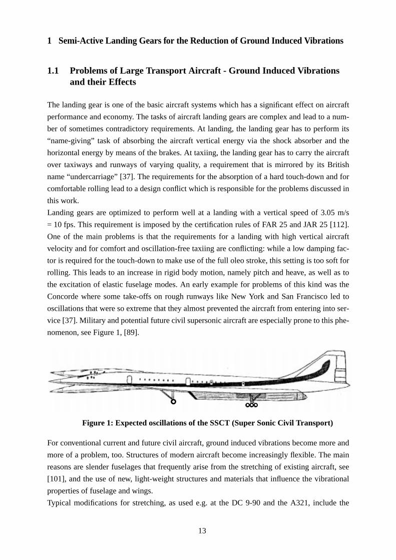
vice [37]. Military and potential future civil supersonic aircraft are especially prone to this p
nomenon, see Figure 1, [89].
For conventional current and future civil aircraft, ground induced vibrations become more
more of a problem, too. Structures of modern aircraft become increasingly flexible. The
reasons are slender fuselages that frequently arise from the stretching of existing aircra
[101], and the use of new, light-weight structures and materials that influence the vibra
properties of fuselage and wings.
Typical modifications for stretching, as used e.g. at the DC 9-90 and the A321, includ
Figure 1: Expected oscillations of the SSCT (Super Sonic Civil Transport)
13

e air-
land-
form
ation
nd-
ase of
spring
uch-
ping
nal
d are
This,
con-
t their
tioned
dard
f land-
lan-
ill the
an
formed
ers
Tanner
editor.
gear
roup
[108],
ecific
ver-
pers
n the
ritish
tail,
insertion of additional fuselage segments [42]. Most of the other important systems of th
craft remain unchanged, though, including very often the landing gear layout. However, a
ing gear that worked well for one aircraft configuration does not necessarily per
satisfactory for a stretched aircraft version. Thus, a landing gear might satisfy the certific
requirements, but might not fit well with respect to the overall dynamics of aircraft plus la
ing gears. Unexpected vibrations can be the consequence.
Critical natural frequencies of a suspension can be changed within certain limits. In the c
the Concorde, for example, the shock absorber was changed to include a dual-stage air
[37]. Main landing gears of large aircraft often are equipped with valves that open at to
down, where the shock absorber stroke velocity is high, thus allowing a different dam
coefficient for landing and taxiing (a so-called “taxi valve”). All modifications at conventio
suspensions have in common that they can only be optimized for one design point an
therefore in principle not able to overcome the basic design conflict mentioned above.
however, is possible with the application of semi-active landing gears and their respective
trol laws as they are described in this work. Landing gears of that kind are able to adap
properties to the motion of the aircraft at any instant.
1.2 Aircraft Suspension Control - The Solution?
There are a number of books and articles of landing gear design which must be men
here. The books of Conway [11], Currey [14], Pazmany [73], and Roskam [82] are stan
textbooks which cover the whole standard landing gear design process from questions o
ing gear location, suspension layout and the selection of tires. An important - German
guage - reference about problems of the aircraft on the ground and landing loads is st
article by König [50]. The “SAE Committee A-5 for Aerospace Landing Gear Systems” is
association of aerospace engineers who are engaged in landing gear design which was
in the frame of the Society of Automotive Engineers (SAE). Thirty publications by memb
of this committee concerning questions of landing gear design have been selected by
and published in [90]. A second volume of papers [91] has been published by the same
Ohly describes in [70] the current state and trends for future developments in landing
design. Further collections of articles have been published by the AGARD (Advisory G
for Aerospace Research and Development) in their conference proceedings CP-484
“Landing Gear Design Loads”.
While all these publications are concerned with landing gear design in general, some sp
publications exist with respect to the simulation of aircraft ground dynamics. An early o
view of computer simulation of aircraft and landing gear is given by Doyle [17]. Further pa
are published in another AGARD volume [109], which, however, has its main emphasis o
simulation of shimmy. Shepherd, Catt, and Cowling describe a program funded by B
Aerospace for the analysis of aircraft-landing gear interaction with a high level of de
14

dyna-
tions
37]
, the
igners,
g gears
Dil-
ride
ula-
such
to land-
reduc-
bomb
ile no
elec-
l have
en loop
ontrol
wide
s well
ns. In
nsions
fully
f ver-
sent-
re oil
ARD
t. One
on on
rove-
ies by
ers is
pt is
y cars
Quite
rack,
] per-
differ-
including brakes and anti-skid, steering control, to simulate standard hardware rig test (
mometer and drop tests) as well as flight tests involving ground contact [86]. Two publica
of the IAVSD (International Association for Vehicle System Dynamics), Hitch in 1981 [
and Krüger et al. in 1997 [57] are state-of-the-art overviews of aircraft ground simulation
latter article also discussing different modeling approaches and tools.
The suspension design conflict mentioned above has long been known to aircraft des
and a number of studies have been undertaken to assess the potential of adaptive landin
to resolve the problem of aircraft-runway-interaction. As far back as in 1972, Corsetti and
low have conducted a study of the potentials of landing gear control to improve ground
[12]. In 1977, Somm, Straub, and Kilner [88] have published the results of a study of sim
tions of three military transport aircraft equipped with simple landing gear modifications,
as dual stage air chambers - values for the pressure have been set to a fixed value prior
ing according to the aircraft weight - and passive by-pass orifices. The authors predict a
tion of CG acceleration (RMS) by as much as 47% on semi-prepared and repaired
damaged runways. Fatigue investigations indicate improvements on austere airfields, wh
improvement can be shown for missions on prepared runways. With the advent of micro
tronics at the beginning of the eighties suspensions with computerized closed loop contro
been subject of investigations because they promise greater improvements than the op
approaches like those of [12] and [88]. Karnopp has published the so-called skyhook c
concept (see chapter 4.2.1) for automotive applications [48]. This concept has found
application in automotive, truck, and railway suspensions, both for research purposes a
as for production vehicles, and has been used for fully active and semi-active suspensio
1984 an AGARD conference has been dedicated to the state-of-the-art of active suspe
[108]. Among the work presented there are the studies of Freymann, who proposes a
active nose landing gear for the reduction of ground loads [26]. He obtaines reductions o
tical acceleration of approximately 42% for a rough runway excitation on a test rig repre
ing aircraft pitch, with considerable technical effort because an external high pressu
reservoir is needed for fully active oleo control. Most investigations presented at the AG
meeting, however, have been dedicated to the reduction of peak loads at landing impac
example is the study of active landing gears for an F-106 fighter aircraft, aimed at operati
an aircraft carrier [39]. Here, also on a test rig with a high pressure oil source, modest imp
ments in the reduction of landing loads can be shown.
Only recently semi-active concepts for landing gear control have been introduced. Stud
Karnopp [46] for automotive applications suggest that the efficiency of semi-active damp
only marginally lower than of a fully active system, provided that a suitable control conce
used. Goodall [63] investigates semi-active suspensions for the lateral damping of railwa
and makes some studies on filtering methods for the use of a skyhook control in curves.
a similar situation arises when a vehicle with vertical skyhook damping drives on a road, t
or - in the case of an aircraft - on a runway with a slope. Catt, Cowling, and Sheppard [8
form simulation studies on active and semi-active aircraft suspensions. They investigate
15

ormal
e, as
mar-
fully
igates
dicts
rame
ration,
ntrol
und
ding
igid
builds
CUS
In that
sed to
Gear
mod-
f the
i-active
well as
oject
efore
d.
tions,
ctive
eeds
t air-
ering
e the
efore
del.
ent feedback strategies, including feedback of pitch rate, pitch acceleration, and n
(vertical) acceleration, the last choice showing the most potential. They also conclud
Karnopp has done, that the improvement of ride comfort for a fully active system is only
ginally better than for a semi-active system and agree not to pursue the investigation of a
active scheme any further because of its high system complexity. Wentscher [101] invest
the use of a semi-active skyhook-controller for an A300 to improve ride comfort. He pre
considerable improvements; however, he works with a relatively simple model of the airf
structure and uses harmonic excitations, at a fixed speed and a single aircraft configu
investigating only slight aircraft weight changes. Duffek [19] develops a semi-active co
concept for the landing impact which could be combined with a control concept for gro
ride. Wang studies a main landing gear model of an A320 with a fuzzy-controller for lan
and rolling, but restricts himself in [98] to a two-mass landing gear model and in [99] to a r
aircraft model.
There have also been practical applications of the technology in road vehicles. Mercedes
its new S-Class with semi-active skyhook damping [80]. In the European COPERNI
project, a truck has been equipped and tested with semi-active shock absorbers [94].
project the main aim has been to show that semi-active shock absorber control can be u
reduce dynamic tire forces which are a main cause of road damage.
In the course of another European project, ELGAR (European Advanced Landing
Research, [107]), Liebherr Aerospace Lindenberg has built a test-rig demonstrator with a
ified helicopter nose landing gear on a vertical shaker to prove the technical feasibility o
semi-active damping concept for aircraft.
1.3 An Integrated Design Process for Semi-Active Landing Gears
Even though a considerable amount of research has been performed on the topic of sem
suspensions in general, discussions with airframers and landing gear manufacturers as
experience gained in the course of ELGAR and the German national Flexible Aircraft Pr
[59] led to the identification of a number of open problems which have to be addressed b
the implementation of semi-active landing gears on production aircraft can be considere
It is the intention of this thesis to give answers to some of the most important open ques
most notably concerning the choice of a suitable controller, the influence of the semi-a
control on aircraft flexible modes and the behavior of the controlled aircraft at different sp
and different weight configurations.
To be able to examine these topics not only for a “generic“ but also for a technical relevan
craft, it is vital that it is possible to combine submodels of different partners and engine
disciplines which are involved in the design of the aircraft concerned to be able to analyz
complete model. For the evaluation of aircraft-landing gear dynamics, this thesis ther
makes use of concurrent engineering methods for the development of the simulation mo
16

alysis
oderate
lysis
de can
nt, bi-
prop-
ation
design
zzy-
l and
ecause
ontrol.
a fur-
to the
dence
ircraft
ns are
hile
nose
d the
ell as
hile a
xcita-
often
estion
all.
romise
trol
. Fully
ure res-
k will
g the
tional
ar will
refer-
thods
role
Multibody simulation has been chosen as the method for model set-up, simulation and an
because it allows a good mean between the requirements of high model accuracy at a m
model complexity as well as low computation times. It also offers a large number of ana
methods in both the frequency and the time domain. Furthermore, the used multibody co
be connected to other tools from the concurrent engineering area by a number of intellige
directional interfaces.
The following analysis strategy is employed in the thesis: the airframe and landing gear
erties are determined by importing elements from finite element models, multibody simul
models and measurements. An interface between the simulation program and a control
tool is developed. Using this interface, three control laws, a skyhook-type controller, a fu
logic controller, and a state feedback controller, are developed in the control design too
exported into the simulation environment. These control strategies have been selected b
they have been shown to be effective in semi-active automotive and truck suspension c
The control parameters are optimized using a multi-objective parameter optimization. In
ther step, the performance of the three control strategies is compared with respect
improvement of vertical accelerations in the time- and the frequency-domain. The depen
of the control performance as a function of system parameters, regarding both varying a
speed and aircraft weight, is assessed, and limitations due to realistic actuation restrictio
discussed.
The investigation will concentrate on rolling. Semi-active control of the touch-down, w
feasible, will not be touched. The study concentrates on the semi-active control of the
landing gear only. Because of its location a the long distance from the center of gravity an
main landing gear, vibrations of the rigid body modes (especially the pitch mode) as w
elastic fuselage and symmetric wing modes can be influenced and damped effectively. W
control of the main landing gears could also be envisaged, especially since much of the e
tion is induced via those gears, they are subject to high inner sliding and stick friction,
due to strong bending because of high leg inclination angles. It is, therefore, an open qu
whether control of the main landing gears will lead to reduced accelerations or loads at
The semi-active control concept has been selected because it offers a good comp
between complexity and efficiency, i.e. it combines low additional weight with a good con
performance. Furthermore, semi-active shock absorbers can easily be designed fail-safe
active systems require a lot of additional equipment because of the necessary high press
ervoir, leading to a weight penalty and reliability concerns.
The thesis is structured according to this analysis strategy: the presentation of the wor
start with an overview of landing gear requirements and configurations, also highlightin
above-mentioned design conflict between touch-down and rolling (chapter 2). Conven
passive landing gear concepts as well as a proposed design for a semi-active landing ge
be discussed. This chapter will also point out why a semi-active solution has been given p
ence over a fully active one. Afterwards, modern landing gear design and simulation me
will be discussed, especially the use of multibody simulation which will play an important
17

ween
rtant
given
e crite-
craft
ct to
e dis-
cessary
oach.
eters
el is
con-
. The
of the
ontrol
design
ed at
in this investigation. The most important software tools used including the interface bet
multibody simulation and control design tool will be presented.
In chapter 3 the aircraft and landing gear model will be discussed in detail. The most impo
equations for the force laws necessary for the simulation of the system dynamics will be
as well as the used configurations, the excitations used for design and evaluation, and th
ria for the optimization of the control parameters. The two-mass model and its role in air
suspension design will be introduced. Finally, an analysis of the aircraft model with respe
observability and controllability will be performed.
In chapter 4 the control design is performed. The possibilities for suspension control ar
cussed, the theoretical approach to the three selected control laws is given as far as ne
for the work, followed by a discussion of the restrictions imposed by the semi-active appr
The design process of the controllers and the optimization of the respective control param
are shown at the end of the chapter.
The performance evaluation is the topic of chapter 5. A simulation of a full aircraft mod
performed, first for the design point, then for different aircraft speeds and aircraft weight
figurations. The semi-active approach is compared with a possible fully active design
results are evaluated with respect to time and frequency criteria. Technical aspects
implementation, as actuator force level and response time, are discussed. Finally, the c
concepts are compared by regarding not only their respective performance but also their
and implementation effort. Open questions which arise during the work will be address
the end.
18

n as
per-
have
most
ara-
s for 3
ight
aths in
table
the
c and
of the
ears.
tire
port.
tons
This
limited
ossess
les in
ased in
.
land-
Load
lly at
ding
case
f the
ny air-
ateral
2 Landing Gear Development as an Integral Part of Aircraft Design
2.1 Aircraft Landing Gears: Requirements and Configurations
2.1.1 Landing Gear Requirements
Aircraft landing gears fulfill the tasks of absorbing the vertical energy of the touch-dow
well as providing a smooth ground ride before take-off and after landing. However, they
form a number of further duties which are less evident. Jenkins [43] and Young [104]
given a detailed presentation of these requirements which are summarized in [57]. The
important factors influencing the landing gear design are described in the following p
graphs.
System weight is an important aspect in aircraft development. The landing gear account
to 6% of the maximal takeoff weight. A subsequent major reduction in landing gear we
will be hard to realize because the landing gears are one of the few non-redundant load-p
an aircraft, and any reduction in reliability from current fail-safe standards is not accep
[10]. Considering the progress in aircraft light-weight structural design and fuel efficiency
relative weight share of the landing gears can thus be expected to increase further.
The position of the landing gears must be such that the aircraft will not tip over under stati
dynamics loads. Another important factor for the design is the number and properties
tires as airfield compatibility has become an important factor in the design of landing g
The number of tires depends on aircraft weight, maximum force per tire and maximum
size, and is dictated by pavement bearing strength which may vary from airport to air
Large civil transport aircraft as the A340, Boeing 747 and MD 11 reach loads of over 20
per tire on the main landing gears.
During flight the landing gears of practically all modern transport aircraft are retracted.
requires restrictions on the landing gear positioning as these parts have to be stored in a
space and must not collide with other systems. For this reason, landing gears often p
complicated kinematical layouts of the retraction mechanism for the storage in nacel
wings and fuselage. Landing gears are usually retracted to the front so they can be rele
case of a hydraulic failure and being pushed into position by the air flow, Figure 2, [101]
Since landing gears have to carry the aircraft weight and have to absorb the energy of the
ing impact, the fuselage has to be strengthened in the vicinity of the attachment points.
alleviation is therefore also of importance for the dimensioning of the fuselage, especia
the attachment points and at the rear of the aircraft. For aircraft with a high maximum lan
weight the bending moment resulting from the landing impact is often the critical design
for the rear fuselage [59]. Therefore, comfort improvements obtained by the application o
results of this study must not result in higher attachment loads.
Other load cases besides touch-down and rolling are also of great importance. On ma
ports aircraft are towed, either by push-rods or by special trucks. Cornering exerts high l
19

ined at
sider-
rcraft
DOCs
main-
con-
e per-
nsion
rn air-
cated
sions
war
cy by
that
com-
, the
ce the
loads on the landing gears. These factors often lead to higher forces than those obta
touch-down, especially in lateral and horizontal directions, and have to be taken into con
ation as design loads [112].
All requirements mentioned so far have to be met with a system that is one of the few ai
parts which have no redundancies. And, as airlines look as well at acquisition costs as at
(direct operational costs), the landing gear should be inexpensive and require minimum
tenance.
The great number of requirements can only be fulfilled if comprehensive trade-off studies
cerning space availability, weight considerations, and structural (stress-) evaluations ar
formed. Since a large number of engineering disciplines are involved in the suspe
development, an integrated design of airframe and landing gears is essential for mode
craft.
2.1.2 Landing Gear Configurations
Landing gears have developed from the simple skids of the first aircraft into the sophisti
and rather complex systems they are today. Originally, the spring function of the suspen
consisted only of the leg elasticity or solid springs [104]. In the years after the first world
the oleo-pneumatic shock absorber became popular because it provided high efficien
combining the desired spring and damping characteristics in a relatively small unit. At
time, the landing gear configuration with two main landing gears and a tail wheel was
mon, the most prominent example being the DC 3, see Figure 3a, [56]. In the thirties
retractable landing gear was introduced for reasons of reduced aerodynamic drag. Sin
Figure 2: A300 nose landing gear
FWD
20

t has
nding
d L-
nclude
ircraft
n com-
ound,
er of
f the
and
nd-
t the
cation
ing to
generation of aircraft of the fifties the landing gear configuration of large transport aircraf
remained principally the same - a steerable nose landing gear and two, or more, main la
gears [14], one of the earlier aircraft with landing gears of that type being the Lockhea
1049G Super Constellation, see Figure 3b, [56]. Other possible landing gear systems i
floaters, skids, skis, track-type gears, and air cushions. They are applied in specialized a
but have found no wide usage [81], [90].
The nose wheel tricycle landing gear configuration has some important advantages whe
pared to the tail wheel type gear. First, the fuselage is level when the aircraft is on the gr
increasing visibility for the pilot at take-off and at ground maneuvers. Second, the cent
gravity is located in front of the main landing gears which leads to a pitching moment o
aircraft at touch-down, automatically reducing lift. Furthermore, the aircraft is stabilized
the pilot can utilize the full brake power [10]. On the other hand, aircraft with tail-wheel la
ing gear types have an initial angle of attack, allowing a shorter take-off distance.
A major disadvantage of the conventional landing gear layout, though, is the fact tha
requirements mentioned in section 2.1.1 restrict the designer’s choice of landing gear lo
and layout. With aircraft becoming larger and the number of main landing gears increas
Figure 3: Common landing gear configurations
a) tail wheel landing gear configuration: DC 3
b) nose wheel tricycle landing gear configuration: L1049G
21

ilable
d sta-
main
mmo-
chal-
nose
ulti-
gie. In
e land-
r acts
rs with
to sta-
h is
atic
ergy,
hock
ch is
and an
) and
stroke
three or even four, substantial limitations in the designer’s freedom occur [10]. The ava
envelope within which the landing gear has to be located to produce the ideal loading an
bility characteristics may no longer be large enough to place the increased number of
landing gears in the fuselage and the wings. A good example is the A380 where the acco
dation of four main gears with four- and six-wheel-bogies poses a demanding design
lenge.
2.2 Conventional, Active, and Semi-Active Landing Gears
2.2.1 Conventional Landing Gears
Practically all modern transport aircraft are designed with retractable landing gears in
wheel tricycle configuration. The main landing gear is equipped with disk brakes and a m
tire combination on one or several axles. In the latter case the axles are connected to a bo
many cases the shock absorber acts in the (vertical) translational degree of freedom of th
ing gear (cantilevered gear, Figure 4a, [74]); in another type of gear, the shock absorbe
across a landing gear angle (articulated gear, Figure 4b). A number of nose landing gea
the shock absorber in the translational degree of freedom are designed with a small trail
bilize the wheel while taxiing. An example is the A300 nose landing gear in Figure 2, whic
of the same configuration as the nose landing gear used in this work.
Almost all commercial transport aircraft today are equipped with an oleo- (i.e. oil-) pneum
shock absorber, often simply called the “oleo” to absorb and dissipate vertical kinetic en
see Figure 5, [101]. An oleo has a high weight efficiency when compared to other s
absorber types. It consists of a chamber (1) filled with gas (mostly dry air or nitrogen) whi
compressed during the stroke and provides the characteristics of a progressive spring,
oil volume which is pressed through orifices between main chamber (2), gas room (1
recoil chamber (3) at compression and expansion to account for the damping of the
Figure 4: Shock absorber configurations
a) cantilevered main landing gear b) trailing edge (articulated) main landing gear
bogie
shock absorber
22

of the
ding
tical
ure 6
by the
g and
point.
these
oreti-
t (i.e.
motion. Friction is introduced by two phenomena, the pressure of the seals on the metal
fittings (“seal friction”) and the strong bending moments, especially at touch-down (“ben
friction”) and can account for more than 10% of the total force in the oleo (for a mathema
representation of friction models see section 3.3.4).
This layout leads to a relation of force over stroke during the landing impact shown in Fig
[104].
The areas under the load-stroke curve in that figure correspond to the energy generated
respective forces. The spring force increases with stroke, storing energy. The oil dampin
the friction forces dissipate energy until the system comes to rest at the static closure
Figure 7a shows the same process as a function of time for a fixed-orifice oleo. From
considerations follows that the peak force for a landing impact in the shock absorber the
cally reaches a minimum if the area under the load-stroke curve for a hard landing impac
Figure 5: The passive oleo
Figure 6: Characteristic force diagram for landing impact
to airframe
to wheel
gas room (1)
metering pin
oil
fitting
recoil chamber (3)
main chamber (2)
seals orifice
23

ngle; in
For a
ce a
force
f the
thus
n be
r if the
of the
ide a
lose
slope,
sus-
gers or
ping
an for
own.
osed a
a taxi
stroke
flow
i.e.
an impact where the peak force is greater than the static force) has the shape of a recta
the load-time curve, the two peaks of the total force should converge into a single one.
soft landing, in the load-stroke curve the optimum is a force sloping to the static point. Sin
rectangular force level is neither technically feasible nor desirable, as it would lead to a
step, the oleo is optimized to a steep force slope after ground contact, see Figure 7b.
The conventional technical solution for such a shaping of the force slope by a variation o
damping factor is the use of a “metering pin”, which changes the orifice cross section and
the damping factor as a function of stroke, reaching efficiencies of 80% to 90% [10]. It ca
seen from these considerations that the performance of the shock absorber will be bette
full oleo stroke can be used. This in turn leads to relatively soft damping factors because
high stroke velocity at landing impact.
Next to the efficient absorption of the energy of the landing impact the oleo should prov
comfortable ground ride. This poses two problems: first, at taxiing the aircraft is in or is c
to a static equilibrium. Therefore, the air spring operates in the range of a steep curve
especially for the maximum take-off weight, leading to a very hard suspension. This hard
pension is necessary because aircraft weight variations during the boarding of passen
while loading freight should not result in substantial gear deflections. Second, the dam
required to successfully encounter oscillations has to be considerably larger for taxiing th
landing because the oleo stroke velocity at taxiing is significantly smaller than at touch-d
Aircraft designers have been aware of that design-conflict for many years and have prop
number of measures [12]. A standard solution is the use of a double-stage air spring or
valve, i.e. a spring-supported valve that changes the damping coefficient as a function of
velocity, see Figure 8, [58]. For low stroke velocities, i.e. at taxiing, the valve closes at P1 and
high damping factors are achieved. At touch-down, i.e. at a high stroke velocity, the oil
opens the valve at P2, thus reducing the damping factor. The so-called rebound coefficientdexp
can be set separately fromd1 andd2 and is selected such that the aircraft does not jump up,
rebound, in the case of a hard landing.
Figure 7: Passive Load time curve and optimal load-stroke curve for landing impact
F
stroke
Fstatic
Fo
1: extended2: static3: fully
1 32
compressed
commanded stroke passive stroke
a) passive load-time curvetime
total forceF spring force
damping force
friction force
b) optimal load-stroke curve
24

ced,
s, by
lling.
g taxi-
tick-
und
g that
ding
h fixed
rces in
r to
cteris-
e.g. the
t, and
ber of
g of
eight
l. This
traub,
ilitary
uspen-
odes.
l. The
For the rolling aircraft a further aspect is of importance. Strong friction forces are indu
especially in landing gears with a large inclination angle towards the vertical aircraft axi
the resulting bending moment which cause the oleo to stick even while the aircraft is ro
Measurements show that aircraft main landing gears can lock for several seconds durin
ing. In this case all the suspension deflection is provided by the tires only [57]. Although s
ing due to friction, sometimes called “sticktion”, has a strong influence on the gro
dynamics, reliable data about this phenomenon are difficult to obtain - the reasons bein
either the effect is not sufficiently understood or the data are kept proprietary by the lan
gear manufacturers (or both) [57].
2.2.2 Landing Gears of Variable Characteristics
Conventional landing gears as they have been described above are suspensions wit
spring-damper characteristics. Those passive systems are restricted to generating fo
response tolocal relativemotion, e.g. upper and lower strut of the shock absorber. In orde
obtain an improved performance with respect to comfort and loads, the suspension chara
tics can be made adaptable to aircraft parameters as well as to environmental conditions,
quality of the runway. Active systems may generate forces which are afunction of many vari-
ables, some of which may be remotely measured, e.g. vertical acceleration, aircraft weigh
forward speed. Active suspensions are already state-of-the-art and are applied in a num
automotive and railway applications.
Basically, two different active suspension strategies exist. A first type is an a-priori settin
spring or damper characteristics according to the expected runway quality and aircraft w
prior to touch-down, and keeping those suspension characteristics constant during rol
variant, sometimes also called “adaptive suspension“, has been examined by Somm, S
Kilner in 1977 [88] who used a gas spring with an adaptive pressure which was used for m
aircraft landing on unpaved runways. Another variant of this suspension type are those s
sions of luxury cars which can be switched between sportive and comfortable operating m
A second type is the feedback of vehicle motion and, consequently, a suspension contro
Figure 8: Taxi valve - passive system for improved ground ride
s
doleo
d1
d2
s1 s2
P1
P2
dexplower chamber
upper chamber
oil flow
Fd doleo s2⋅=
(stroke velocity)
25

ibed in
nsor
pension
ay of
istin-
natu-
velers
atural
ors for
a gas
tive
ency,
[80].
tems.
nts. The
gure 9.
e 9a.
ilure,
g, e.g.
n also
tion of
s
basic sensor and control layout is similar for most systems and has already been descr
the seventies and eighties by Corsetti and Dillow [12], Karnopp [48], and Hedrick [33]: a se
at the vehicle measures acceleration and velocity of the sprung mass as well as the sus
deflection, and, via a control law, results in a change of suspension characteristics.
Several ways to classify suspension systems can be found in the literature. A common w
classification is by the bandwidth of the actuators. Prokop and Sharp [76], for example, d
guish between
• very slow active systems, the actuator cut-off frequencies of which are lower than the
ral frequency of the body resonance (i.e. frequency range less than 1 Hz), e.g. load le
and adaptive spring settings;
• slow-active systems, which show cut-off frequencies between the body and wheel n
frequencies of the system (i.e. frequency range between 1 Hz and 10 Hz), e.g. actuat
pitch and roll control; systems like these can be realized by pressure variations of
spring, e.g. Citroën Xantia [29], [13], or adjustable mechanical devices, e.g. Delft Ac
Suspension, DAS [95];
• and fast-active systems, with actuation bandwidth beyond the wheel-hop natural frequ
i.e. frequency range above 10 Hz, e.g variable dampers operating at high bandwidth
In the course of this work the term “active suspension” will always be used for the fast sys
The complete suspension can consist of an arrangement of passive and active compone
active parts can be used in parallel with or as a substitute for passive elements, see Fi
Most technical solutions put the actuator in parallel to conventional components, Figur
This is done for reasons of safety, i.e. to guarantee vehicle stability in case of actuator fa
and to reduce the load on the actuator. Furthermore, a certain amount of inherent dampin
by friction, is present in most cases anyway. For control design purposes, however, it ca
be of use to neglect the passive damping, Figure 9b, or to see the actuator as a combina
all suspension parts, Figure 9c.
Figure 9: Possible arrangements of components for active and semi-active suspension
a)
mus
b)
mus
c)Ms
mus
Ms Ms
mus: unsprung massMs: sprung mass
26

nsors
ation
ay be
) and
way,
ons is
lica-
the
l fre-
work-
ractice
ven
], con-
ergy
pond-
ill be
view.
An improved performance can be achieved by the application of so-called preview se
which scan the runway for obstacles and rough patches and enter this additional inform
into the control loop [85]. Sensors using optical, ultrasound and radar technology are m
applied, however, they pose problems concerning practical application (dirt, accuracy
interpretation of data, e.g. how can a water-filled pot-hole be distinguished from the run
how a cardboard box from a stone... [40]. A good compromise for road vehicle suspensi
to use the motion of the front axle as preview for the rear axle [85]. This strategy is not app
ble to aircraft since the tracks of aircraft main gears are so wide that the information from
nose gear would be of little benefit for potential main landing gear control.
Even optimal suspension control has its limits. First, a suspension realizing an optima
quency isolation between passenger and road or runway input would require an unlimited
ing space. Second, the wheel-hop natural frequency cannot be damped easily since in p
it is difficult to measure the tire deflection. Third, energy consumption limitations apply. E
though extreme opposite standpoints in respect of energy consumption are possible [85
ventional solutions with electro-hydraulic actuators require a substantial amount of en
since actuation occurs by virtue of high pressure oil flowing into the actuator and a corres
ing volume of oil has to be exhausted to tank (atmospheric) pressure (see next section).
Figure 10 gives an overview of the suspension layouts discussed above. This work w
restricted to the control of semi-active suspensions in the range of 1 to 10 Hz without pre
Figure 10: Suspensions of variable characteristics
suspensions
fixed characteristics variable characteristics
single stage multiple stage
systems without feedback
variable spring variable damperslow(load leveler)
medium fast(variable spring)
aktive semi-active
with preview without preview
feedback systems
fast(var. damper)
27

rs are
hock
ever,
craft
flict.
t of it,
emi-
11b,
the
or the
tions
sign of
tuator,
d only
ocity
is
com-
e only a
. The
very
sys-
2.2.3 Semi-Active Landing Gears
As mentioned in section 2.2.1, requirements for the dynamic behavior of shock absorbe
different, even partly conflicting, for landing and rolling. Since certification demands the s
absorber layout for a hard landing, landing gears are optimized towards that goal. How
even this optimization is only valid for a single operational point, i.e. sinking speed and air
weight.
Active (“fully active”) and semi-active shock absorbers promise improvements to this con
Figure 11 exemplifies the differences between those concepts.
In active shock absorbers oil is pumped from a pressurized reservoir into the oleo and ou
responding to the commands of the controller, Figure 11a, [101]. The principle of the s
active oleo consists of regulating the energy dissipation by a controllable orifice, Figure
[101]. Thus, the semi-active control is also known as “active damping” [8]. Contrary to
fully active systems the semi-active oleo requires no external energy supply other than f
control valve. Semi-active dampers are state-of-the-art in railway and automotive applica
[94].
As for a passive damper, the applicable force in a semi-active damper depends on the
the stroke velocity across the damper, see Figure 12. Since, contrary to the fully active ac
the damper can only dissipate energy, not every control command can be applied an
forces can be produced which lie in the first and third quadrant of the force-stroke vel
plane, i.e. a positive forceFd in the sense of Figure 12 can only be supplied while the oleo
compressing, a negative force can be supplied by an expanding oleo. If the controller
mands a negative force during oleo compression, the best that can be done is to generat
compression force as small as possible, in other words, to open the orifice completely
requirement to be able to switch from force generation to near zero force generation in a
short time makes the semi-active damper an inherently highly nonlinear device.
A controller with a semi-active control scheme is often designed as if it was a fully active
Figure 11: Active (a) and semi-active (b) damper
high pressure
CONTROL
CONTROL
oil reservoir
a) b)
28

his is
rely
ters as
ctive
ctive
eme
oper-
o sys-
ments
rance.
nd less
tions.
y the
rgy to
ears
the
pas-
es of
tem. Control commands that lie in quadrant 2 and 4 of Figure 12 are then set to zero. T
known as a “clipped optimal” approach. It will be shown in this work, however, that a pu
clipped optimal design strategy, i.e. operating the semi-active oleo with the same parame
found for the fully active controller, is only sub-optimal.
Another restriction to the clipped optimal assumptions is the fact that a technical semi-a
damper has a minimum and a maximum orifice size for the oil flow, resulting in a respe
minimum and maximum controllable damping coefficient. Therefore, a clipped optimal sch
has to be replaced by a realistic, limited system setting boundaries for the commands and
ating with separately adapted gains.
The use of fully active landing gears has been investigated in several studies [26], [39]. N
tem has actually been introduced on a production aircraft since the performance improve
have not justified the increased system complexity and the additional weight encumb
Semi-active landing gears, however, are not considerably heavier than passive systems a
complex than their active counterparts, and are therefore better suited for aircraft applica
In addition, a semi-active oleo needs only little energy to operate a valve in order to var
orifice cross section whereas a fully active system requires a substantial amount of ene
build up the high pressure oil supply. Very important is the fact that semi-active landing g
can fulfill the important requirement of a fail-safe design. At power loss or malfunction
characteristics of a semi-active oleo are identical to the characteristic of a non-optimized
sive fixed-orifice oleo. Table 1, [101], gives an overview of advantages and disadvantag
the different shock absorber concepts.
Figure 12: Principle of semi-active damping for an oil shock absorber
s (stroke velocity)
Fd
“clipped optimal” region
dmin < dcom < dmax
Fd
Fd
s.
.
Fd d s s⋅=
s > 0: compression
s < 0: extension
.
.
29

Fully
tional
es the
re 13,
oses
meter
of the
ontrol
time
topic,
e oleo.
2.2.4 Control Actuators
All control schemes for suspension control require an actuator in the landing gear leg.
active oleos have been built and tested by Howell et al [39] and by Freymann [26] as addi
hydraulic pressure sources connected to the oleo by supply pipes. While Freymann us
upper chamber for oil exchange, the lower oleo chamber is used by Howell et al, see Figu
[39], [26]. Otherwise, both test actuator set-ups are similar, feeding back for control purp
the information of an acceleration sensor at the top of the landing gear, a linear potentio
for the measurement of the oleo stroke and a pressure gauge for the measurement
hydraulic pressure in the actuator. Servo valves are used to regulate the oil flow.
The dynamic response of the actuators is of special interest for the evaluation of the c
performance. While in [39] no comments are made concerning the actuator response
since the test rig was used for drop-test evaluation and dynamic response was no prime
Freymann notes a significant delay between actuation signal and pressure build-up in th
passive semi-active active
low weight low weight high weight
satisfactory perfor-mance only for designpoint
good performanceover wide opera-tional range
good performanceover wide operationalrange
medium complexity medium complexity high complexity
fail-safe fail-safe fail-safe?
Tabelle 1: Comparison of different landing gear concepts
Figure 13: Active landing gear control
30

o be
he res-
ed by
a car
semi-
5 ms
ime for
t inde-
d by a
ponse
per a
apta-
. The
ctive
gear
ilable
and
5.1.3.
loop
amper
justed
ontrol
er, the
mpera-
ce the
er and
mper
ponse
en loop
mping
.g. for
this
According to [26], the reason for this delay is that a large volume of hydraulic oil has t
inserted into the upper oil chamber of the oleo in order to compress the gas enclosed in t
ervoir before a significant pressure is built up. A phase angle of 90˚ at 0...5 Hz was observ
the author.
Besinger et al [2] investigated the dynamic behavior of a semi-active damper. Using
shock absorber on a hardware-in-the-loop test rig, transition responses for switching of a
active damper were recorded. For the given set-up, a response time of approximately
between the applied control signal and the damper force response was recorded. The t
the damper force to reach its steady state level results in an additional 10 to 15 ms, almos
pendent of the velocity across the damper, indicating that the force transients are governe
stiff linear compliance. Causemann and Irmscher of Sachs Boge reported similar res
times for their automotive by-pass shock absorber design [9]. For a semi-active truck dam
time delay of approximately 5 ms after application of the control current in a phase of ad
tion due to electrodynamics, valve dynamics and oil compressibility could be measured
time to full adjustment was 35 ms for closing and 15 ms for opening [94]. The semi-a
landing gear test rig built up by Liebherr Aerospace consists of a helicopter nose landing
with a modified oleo also equipped with a by-pass system based on a commercially ava
servo-electric valve with a cut-off frequency of 20 Hz [107]. The performance of active
semi-active control as a function of the actuator response time is investigated in chapter
Force control of a semi-active landing gear can be achieved in two ways [2] - open
response, where the damping coefficient is selected for a given demanded force and d
velocity using a look-up table, and force feedback control where the damping rate is ad
according to the error between measured and desired damping forces. Open loop c
requires relatively simple instrumentation to measure the velocity across the oleo; howev
performance of the suspension is subject to changes in damper characteristics due to te
ture variations and wear. Force feedback requires more complex instrumentation sin
damper force needs to be monitored continuously, e.g. by pressure gauges in the upp
lower oleo oil chambers, but it offers the advantage of being insensitive to changes in da
characteristics. It is shown in [2] that the open loop control displays a faster dynamic res
than the force feedback scheme. In the case of the studies performed in this theses an op
control is assumed. The commanded damping force is transformed into a commanded da
orifice cross section, using pre-set values for the mechanical properties of the system, e
oil density. It is one of the important open points to verify in practical tests whether
assumption can remain valid for the whole operational range.
31

mber
ds on
y [11]
n geo-
o the
to be
the
. The
ic and
and
grav-
ng the
con-
oleo
d too
to
e for
brake.
make
le to
sport
or an
rules
Num-
ared
tons
the
nal
e and
ation
indi-
[94].
2.3 Modern Landing Gear Design: Concurrent Engineering and Multi-body System Simulation
2.3.1 Landing Gear Design as a Part of the Aircraft Design Process
The landing gear design is one of the fundamental aspects of the aircraft design [14]. A nu
of engineering disciplines are involved since the quality of a landing gear concept depen
the efficiency of the overall system integration.
The traditional landing gear design process has been described in textbooks by Conwa
and Currey [14]. This process is based on experience and, in its early phase, based upo
metric considerations, i.e. questions of landing gear configuration and its integration int
fuselage and the wings.
At the start of the design process the possible range of the aircraft center of gravity has
determined. This information is required not only for flight mechanics but also to position
landing gear according tol ground stability, maneuverability and clearance requirements
design has to make sure that the vector sum of weight and applied forces under stat
dynamic conditions will not result in a point outside the triangle determined by the nose
the main gears. The aircraft is in danger of tipping over if the distance between center of
ity and the connecting line between the main landing gears is very small, an example bei
Boeing 727 which is mostly parked with the rear airstairs down [10]. At some aircraft this
straint has led to main landing gears which are strongly tilted backwards, resulting in high
friction (see chapter 3.3.4). On the other hand, the center of gravity should not be locate
far to the front in order to allow the aircraft to rotate at take-off. In most aircraft about 85%
92% of the weight is distributed on the main landing gears [10] which is also of advantag
a short stopping distance; in most cases only the main landing gears are equipped with a
The track of the main landing gears is limited by the fact that the aircraft has to be able to
a curve of 180˚ on the runway.
Another important aspect are the mission requirements. A military transport aircraft ab
start on short unpaved runways will require a different suspension layout than a civil tran
aircraft operating from international airports.
As mentioned in section 2.1.1, flotation requirements, i.e. the number and size of tires f
aircraft of a given mass, are essential for aircraft operation on airports. The certification
for encumbrance of paved runways can be found in the Aircraft-Pavement Classification
ber (ACN-PCN) [110]. The ACN of a certain aircraft determines whether an aircraft is cle
to operate out of an airport with a given PCN. As a consequence, for an Airbus A320 (199
MTOW) six wheels are sufficient, an A340 (275 tons MTOW) needs 12 wheels, and
planned A380 (up to 550 tons MTOW) will probably be equipped with 22 wheels. Additio
wheels, however, mean higher landing gear mass; one wheel of an A340 including tir
brake, for example, weighs about 350 kg. Only static tire loads are considered for certific
purposes, no criterion for dynamic loads exists yet. However, studies performed on trucks
cate that improved suspension layout can also lead to reduced dynamic pavement loads
32
ncern-
sis fol-
wing
by the
ears
an be
the
regula-
s the
e dif-
in the
A300,
fulfill
often
com-
velop-
ps the
d for
hole
aft is
n
and
rav-
ight
of
scent
In a further step, the shock absorber is designed. The most important considerations co
ing the shock absorber design have been discussed above in chapter 2.2.1. A load analy
lows as landing gear loads are decisive for much of the fuselage. While the wings and the
spar frame are dimensioned by gust loads the fuselage aft section is often dimensioned
bending moment resulting from the impulse of the landing through the main landing g
[59]. Finally, the retraction mechanism has to be designed and a first weight estimation c
given.
Many decisive criteria like number of tires and brakes for flotation analysis as well as
shock absorber design must be defined considering international standards and design
tions as the above-mentioned ACN-PCN [111] and the FAR/JAR 25 [112]. This make
landing gear one of the key systems in the pre-design, as a change of configuration will b
ficult and costly late in the development phase. Two examples for such a late change
design have been the third main landing gear on the fuselage of the DC-10-30 and the
where the wheels were placed further apart on the bogie which was mainly necessary to
the runway load requirements of New York LaGuardia Airport [10].
Since the design and production of a large aircraft requires enormous manpower and
extremely specified know-how, aircraft and landing gears are often designed by different
panies. After the specification of the requirements and the basic geometrical data the de
ment and production of the landing gear is given to a specialized company which develo
gears according to the airframer’s specification and the certification requirements.
At present, the main certification requirements for the landing gear design are formulate
the whole aircraft and for the single landing gear. The ground load requirements for the w
aircraft can be found in FAR/JAR 25.471 ff. The manufacturer has to prove that the aircr
able to withstand a landing at the following conditions:
• The aircraft is in a steady state prior to touch-down.
• The landing is symmetrical, i.e. no roll and no yaw angle.
• The descend rate is 10 ft/s = 3.05 m/s at maximum landing weight (MLW).
• The horizontal speed is Vl1 (= stalling speed Vs0 at sea level, about 70 m/s for aA340).
• Calculations have to be performed for minimum pitch angle, “three-point landing”,for maximum pitch angle, “tail-down landing”.
• as well as for critical (extreme for and aft, vertical and lateral) aircraft centers of gity.
• The descend rate is 6 ft/s (= 1.83 m/s) at a landing with maximum take-off we(MTOW).
• Aircraft lift may be assumed to exist throughout the landing impact; no bottomingany of the energy absorbing elements may occur.
• A dynamic response of the structure must be covered by an analysis at a limit develocity of 10 ft/s for the complete flight structure.
33

n bygearti-
cityice,e air-
gears
anda-
substi-
ary
ics of
struc-
ynam-
ation
is the
ding
ency:
and
inter-
es a
atives
nt as
s have
nown
. The
arch.
asure-
if the
tches.
per-
fifties
exist
cases
still
The landing itself gear has to fulfill the requirements of FAR/JAR 25.721:
• The limit load factors of FAR/JAR 25.721 must not be exceeded. This must be showenergy absorption tests, either with a complete aircraft, or with a complete landingin a drop test from 18.7 in (for MLW) and 6.7 in (for MTOW) with an equivalent substutional mass.
• Additionally, the landing gear must be able to withstand a landing at a vertical veloof 12 ft/s (= 3.66 m/s, drop test from 27 in) at a horizontal velocity of zero; in practsink speeds of this magnitude rarely occur due to ground effect and flare-out of thcraft prior to landing.
Next to simulation and excessive calculations with finite element models of the landing
the manufacturers perform a number of practical tests. As seen above, drop-tests are m
tory, as well for verification of the loads as for fine-tuning of shock absorber parameters.
In the landing gear simulation and at the drop-test the aircraft is usually represented as a
tutional mass. Lift is simulated by simple force laws in the simulation and with auxili
means, e.g. aluminum bee-hive structures at the test rig [90]. It is evident that the dynam
the airframe are included only inadequately which can lead to unwanted influence of the
tural elasticity on the loads and, vice versa, of unexpected influence of the landing gear d
ics on the natural frequencies of the aircraft. However, there are only a few certific
requirements for rolling, most of them concerned with braking and turning [112].
It should be mentioned at this point that another decisive factor for loads and dynamics
aircraft tire. Modeling the tire characteristics is a science for itself. Tire models vary depen
on load direction (vertical and lateral models) and frequency range of interest (low frequ
e.g. touch-down, braking, turning; high frequency: e.g. shimmy). In 1941, von Schlippe
Dietrich [84] have analyzed the shimmy motion of the aircraft and have described the
action of tire and landing gear leg stiffness with tire forces analytically. Pacejka [71] us
similar tire model based on the stretched string concept and developed simple deriv
representing first order lag with a relaxation length and a gyroscopic couple coefficie
parameters. For the description of steady state slip characteristics empirical expression
been developed by Bakker and Pacejka [1], using trigonometric functions; this model is k
as the “Magic Formula”. Recently this model has been extended to dynamic tire forces
tire model of Moreland [68] is also frequently used in aircraft landing gear dynamics rese
Reference [72] gives an overview of tire models used in vehicle dynamics analysis.
Independently from the theoretical approach, tire models have to be validated by me
ments on drums or test trucks. Results differ widely between test methods and, even
same methods are applied, between tires of the same type from different production ba
Additionally, tire properties depend on tire pressure, wear, and external conditions like tem
ature and road or drum surface properties. Also, while a lot of testing dating back to the
has been performed for radial tires [87], only few validated theoretical models of bias tire
even though they have been successfully used on aircraft for many years. Thus, in many
today’s tire models are sufficient for simulations giving trends, but many questions are
open to research, if precise results are expected from simulations [57].
34

lead to
s have
d on
ircraft
arable
onic
lation
prob-
nt due
rated
pres-
ers as
the
umber
isci-
O of
pre-
most
ics,
ional
ody
ers a
How-
cation
was
tions,
finite
the air-
le by
dition,
t is in
edun-
3].
The conventional landing gear layout process is well understood and has been proven to
satisfactory designs in most cases, even though a number of last-minute modification
been necessary for production aircraft [10]. However, newly developed aircraft will depen
more integrated design approaches for light and reliable designs, especially if novel a
concepts are concerned for which classic approaches might not applicable and no comp
experience is available. This will be the case for the Airbus A380, for a potential Supers
Civil Transport Aircraft [81] and especially for blended wing-body configurations.
An essential element of new design methods will be an exchange of models and simu
results between the involved disciplines and manufacturers at all design stages to identify
lems of system integration that might lead to expensive re-design late in the developme
to unsufficient load prediction or unexpected fuselage vibrations. Aspects of such integ
design methods are discussed in the next sections.
2.3.2 Multibody Simulation in the Concurrent Engineering Process
At the development of a new aircraft, engineers of several disciplines are involved, under
sure of decreasing development time and of limited financial resources. As manufactur
well as civil and military customers try to incorporate multidisciplinary design methods in
conceptual design phase [36], a more systematic approach needs to be introduced. A n
of projects and programs aim at providing the designer with tools to automate the multid
plinary analysis. Examples of this development are the programs MIDAS and MEPHIST
Daimler Benz Aerospace Airbus [78], [79], and the more landing gear oriented package
sented by Chai and Mason [10].
Modeling and computer simulation have become tools in all engineering disciplines. The
widely used are computer aided design (CAD), finite element analysis (FEA), flight dynam
control design (often called CACE - Computer Aided Control Engineering), and computat
fluid dynamics (CFD). A mediating role between these disciplines is taken by the multib
simulation (MBS) approach. It aims at the simulation of the total aircraft dynamics and off
good compromise between “fast”, “robust”, and “exact” simulation [83].
All those methods can be summarized by the term “computer aided engineering” (CAE).
ever, the models used in the engineering fields differ considerably depending on appli
and the complexity of the task. As an example, in “classical” flight mechanics the aircraft
often represented as a point mass (the coupling of flight mechanical and structural oscilla
of course, today demands a more detailed modeling). Contrary to that, the methods of the
element analysis and computational fluid dynamics decompose structure and surface of
craft in millions of small computational units, a development that has been made possib
the powerful improvement of computer hardware and software in the last decades. In ad
modern CAD programs allow the design of a virtual prototype before a single componen
production. However, this large versatility of models requires an enormous, sometimes r
dant modeling effort, and makes it difficult to exchange the obtained results [32], [83], [9
35

terac-
sical”
cha-
es of
indis-
rtant
and
o per-
oring
ata
is of
se on
p for
lation
m is
atically
ese
s of
ge of
, as an
ment
ing of
make
ong all
n the
indus-
Ero-
xible
er-
inte-
rience
edi-
loads
alists,
odel
at the
Furthermore, the advent of microelectronics into mechanical engineering led to a close in
tion between mechanical and electronical components. This combination of the two “clas
disciplines, mechanical and electronical engineering, led to a new discipline, called “Me
tronics” [52]. In these kind of systems the dynamics are not only determined by properti
the mechanical components but also of the control design.
For mechatronic systems an integrated design of mechanical structures and control is
pensable. Multibody simulation is well suited for this procedure and is therefore an impo
tool in the concurrent engineering process. Multibody simulation allows model simulation
analysis using the know-how of all engineering disciplines mentioned above. To be able t
form these tasks, the program needs intelligent bi-directional interfaces to tools of neighb
disciplines like CAD, FEA, and CACE which allow a continuous comprehensive d
exchange. Multibody simulation is suitable both for the pre-design and for the analys
existing systems, and can be applied for stability and comfort analysis, aircraft respon
certain maneuvers, for ground and gust loads, and for life-time prediction. A further hel
the design process is the possibility to perform parameter studies on a complex simu
model and to optimize free parameters (“design-by-simulation”). Finally, an MBS progra
used to calculate system response in a large number of critical operational cases autom
which is of advantage for certification cases. A multibody simulation tool which fulfills th
requirements is an essential part of the integrated design process.
During the development of an aircraft it will frequently be the case that the modification
one engineering group will lead to a change in the configuration and, therefore, to a chan
the complete system dynamics. Modifications can have influences on other components
example will illustrate: a modified landing gear can result in increased loads at the attach
points between landing gear and structure and enforce a recalculation of the dimension
the structure. The example presented in section 2.3.3 shows that it is not sufficient to
fixed assumptions about the system at an early point - a concurrent model exchange am
related disciplines has to become the rule. Only in this way the effects of local changes o
whole aircraft can be assessed.
Concurrent engineering methods are developed in national and international projects by
try and research. In the field of aeronautics the EU-program ENHANCE (ENHanced A
Nautical Concurrent Engineering) [106] has to be mentioned, on a national level the Fle
Aircraft Project [59], and on an industrial level the Airbus ACE (Airbus Concurrent Engine
ing) program [65].
This thesis is a contribution to the concurrent engineering process, particularly to the
grated design of aircraft and landing gears. Much of the modeling work is based on expe
gained in the Flexible Aircraft Project. In this project, the DLR played the role of an interm
ate between airframer and landing gear manufacturer who are interested in airframe
(respectively landing gear loads) and certification. Using the model expertise of the speci
i.e. an finite element model of the structure supplied by the airframer and a landing gear m
supplied by the landing gear manufacturer, DLR developed methods and software to help
36

Multi-
cal-
f the
h-down
of a
e used
ircraft
e inter-
yses.
air-
figura-
ations
immy
aly-
exchange of know-how, models and results between the partners (see Figure 14, [59]).
body simulation played an important role at this project as the central analysis tool for the
culation of ground loads for touch-down and taxiing. In a case study for the functionality o
process, a conventional two-stage passive shock absorber has been optimized for touc
and taxiing and has been evaluated against a semi-active nose landing gear oleo.
Initial results of the thesis, i.e. the development of interfaces and a preliminary evaluation
semi-active nose landing gear, have been included in the integrated design process to b
in projects such as the Flexible Aircraft and ELGAR.
2.3.3 Simulation in Landing Gear Design
The discussion in the section above shows that simulation plays an important role in a
development and is essential for landing gear design. Simulations are used to assess th
action of subsystem dynamics and to perform ride quality studies as well as “what-if” anal
Simulation of vertical motion, e.g. the drop tests of landing gears and full (usually rigid)
craft models, are performed to obtain the design loads which are necessary for the con
tion of the landing gear structure and the oleo layout. Of great importance are also simul
of the lateral landing gear motion to assess the lateral landing gear stability against sh
[57]. All these simulations also a part of the certification process.
In this context it is important to choose the appropriate model complexity for the given an
Figure 14: “Flexible Aircraft“: an application of the integrated design process
Airframer Landing Gear Manufacturer
FE - model MBS / CAD -model
modalanalysis
MBS - model:aircraft +landing gear
dynamic analysissimulation
oleooptimizationtouch-down
oleooptimizationtaxiing
oleooptimizationtaxiing
control design
DLR
loads + optimal parameter set
(passive) (passive) (semi-active)
37

odels
model
are
prob-
ection
epre-
s the
dis-
en that
ccel-
xible
s been
way
e cer-
oorly
s com-
for the
istinct,
simu-
finite
rcraft
odes
ADS
of
sis purpose. Traditionally, for the computation of landing gear dynamics, rather simple m
as two-mass models or rigid body models have been used. However, the choice of the
complexity can have a strong influence on the validity of the results. Simplified models
valid in certain ranges only. The simulation presented in Figure 15, based on a realistic
lem, exemplifies this observation: a high-speed taxi over a double (1-cos)-bump (see s
3.4) has been simulated with two models of a large transport aircraft. The first model r
sents mass and moments of inertia for a rigid body aircraft, the second model include
structural dynamics of fuselage and wings up to 20 Hz. The rolling velocity is 60 m/s, the
tance between the bumps 21.2 m, their height 3.8 cm. Regarding the results it can be se
the vertical cockpit acceleration calculated with the rigid model are only one third of the a
erations predicted by the flexible model. This is due to the fact that the first fuselage fle
mode is excited by the bumps and dominates the system response. This behavior ha
observed at existing aircraft which might hit a certain critical frequency at any bad run
[37]. The example shows that the use of simple models, which are sufficient to satisfy th
tification rules according to FAR 25, can lead to misleading predictions and thus to a p
tuned suspension. It is therefore important to select a model as simple as possible but a
plex as necessary.
A number of simulation packages have been developed in recent years which are used
purpose of landing gear simulation. The origins, aims, and usage of the programs are d
resulting in different approaches to the modeling of landing gear dynamics.
Three software packages based of different modeling philosophies which are used in the
lation of aircraft on the ground have been described in [57]. MECANO is based on the
element code SAMCEF, SD-Approach is a tailor-made package for the simulation of ai
ground dynamics, SIMPACK is based on a multibody simulation approach. Also other c
exist for these applications, [49], [27], among those the commercial multibody codes D
[62] and ADAMS [25]. In this thesis, SIMPACK, as the central MBS simulation software
DLR has been selected for modeling and simulation.
Figure 15: Simulation results for a rigid and an elastic aircraft model, taxiing over twosinusoidal bumps at a speed of 60 m/s
flexible aircraft modelrigid aircraft model
time [s]
vertical cockpit acceleration [g]
0.5 1.0 1.50 2.0
-.4
-.2
.0
.2
.4
-.6
.6
SIM PACK
rigid aircraft
flexible aircraft
38

ontrol
es an
e pre-
l law
om-
inside
large
del is
lation
S and
ysical
oded,
modi-
have
used
stic
2.3.4 Methodology of Simulation, Control Design and Analysis
This thesis has three central parts - aircraft and landing gear modeling (chapter 3), c
design (chapter 4), and performance evaluation (chapter 5). The following section provid
overview of the chosen approach. The software packages which have been used will b
sented in detail below.
Modeling and Data
As the central tool for the complete process cycle from modeling to analysis of the contro
performance the multibody simulation tool SIMPACK is chosen. The integration of the c
plete model as well as analysis and optimization of control parameters were performed
this tool.
A major model basis is a condensed finite element model of the fuselage and wings of a
transport aircraft which has been supplied by the aircraft manufacturer. This airframe mo
transferred into the simulation by the pre-processor FEMBS, see section 3.2.1. The simu
model of the landing gears has been set up by the landing gear manufacturer in ADAM
has also been transferred to SIMPACK, section 3.2.2. Force elements describing the ph
properties of the shock absorber are taken from SIMPACK library elements or are user-c
section 3.3. The tire model is also based on a SIMPACK library element which has been
fied by a comparison with measured data supplied by the airframer. The runway data
come from the same source; data for two runways profiles are available which can be
directly in the simulation, section 3.4. All modeling information, i.e. MBS elements, ela
data, runway profiles, are stored in a central project data base.
Figure 16: Aircraft model data sources
fuselage / wings
tire model
oleo (user defined force law)
landing gear models
runwaycontroller
(from CACE)
(from FEA)
(measured data)
common data base(measured data)
(from MBS)
39

els
AX
s are
ntrol
of the
and
the
PS
section
control
multi-
ise”
fur-
ed on
alua-
ita-
tool
difi-
pled
their
ction
used in
rams
nd
a typ-
stems
is of
are
DEs)
n the
Control Layout
The control design is performed by using SIMPACK and MATRIXx in parallel. Design mod
of different complexity are derived from the full model which are transferred via the SIM
interface, section 2.3.5, to MATRIXx’s SystemBuild simulation environment.
The controllers are set up and tested completely in MATRIXx. After the design, controller
exported as force elements from MATRIXx, section 4.3. Using this interface, complex co
structures can be implemented in SIMPACK.
A special contribution by the author to the process used in the thesis is the development
SIMAT interface which enables the transfer of models and controllers between MATRIXx
SystemBuild on the one side and SIMPACK on the other side, see section 2.3.5.
Multi-Objective Optimization:
As a final part of this investigation the optimization of the control parameters using
SIMPACK full model for different load cases and speeds with the program SIMPACK-MO
is performed. Because of the strong nonlinearities in the semi-active suspension (see
3.3.3) and the quasi-stochastic nature of the excitation (see section 3.4), the final sets of
parameters have not been derived by linear control design methods but rather by
objective parameter optimization [44]. This optimization method finds a “best comprom
between several conflicting criteria. The algorithm tries to reduce all criteria such that no
ther criterion can be improved without deteriorating the others. Here, optimization is bas
time integrations of the mechanical system. Those time integrations for simulation and ev
tion are performed in the multibody simulation (MBS) tool where all nonlinearities and exc
tions can be modeled in detail; furthermore, the highly optimized integrators of the MBS
allow rather short integration times. The optimization part, minimization of criteria and mo
cation of the model, is done in a multi-objective parameter optimization (MOPO) tool cou
to the MBS tool. The free system parameters are varied by the MOPO routines within
given limits until an optimal compromise between the criteria is found; for details see se
4.3.2.
Software Tools
As we may see from the procedure, several commercial software packages have been
the course of this thesis for modeling, simulation and control design. The applied prog
will be presented briefly in this section.
SIMPACK is the central MBS simulation program of DLR. It is applied in the areas of air- a
space technology, vehicle system dynamics and robotics. SIMPACK has developed from
ical multibody code to an extensive simulation and analysis package for mechatronic sy
with a number of interfaces to other programs of the integrated design [52], [83]. Bas
SIMPACK is a multibody formalism which generates the equations of motion. Systems
described in relative coordinates. The result is a set of ordinary differential equations (O
or, in the case of kinematic loops, differential-algebraic equations (DAEs). For analysis i
40

the
this
ations
back-
ture
hods
e ele-
s, have
stems
also
ation
rior to
or in
onal
ia the
d for
time domain SIMPACK offers a number of different integrators which are optimized for
use in numerical simulation of mechatronic systems. For all time simulations performed in
thesis, an integrator based on ODASSL, a standard solver for differential-algebraic equ
[5], has been used. This integrator is a variable step size, variable order solver based on
ward differential formulae (BDF) with root functions which has been adapted to the struc
of multibody systems.
Beyond the solvers for time-integration a number of additional numerical analysis met
being part of the program have been applied, in particular for linear system analysis, the
linearization, eigenvalue calculation, and frequency response analysis.
The model set-up is performed using elements from the library of bodies, joints, and forc
ments. Additional user elements, describing the complex suspension force characteristic
been defined using FORTRAN and C subroutines. For the simulation of mechatronic sy
SIMPACK includes a library of elements for the realization of control loops which has
been used; for sensitivity and design calculations parameter variation allows the modific
of up to three parameters in a loop which has been applied for parameter range checks p
the optimization runs. Results of the simulations can be visualized in a 3D-animation
form of data plots.
SIMPACK is included in the concurrent engineering process by its intelligent, bi-directi
interfaces, see Figure 17. Flexible structures are included in the multibody simulation v
pre-processor FEMBS (see section below). The interfaces to MATRIXx have been use
control layout and have been extended as part of this thesis.
Figure 17: SIMPACK in the Concurrent Engineering Process
FEMBSProSIM
numerical
CACE
optimization
Pro/ENGINEER ANSYS
MatrixXMOPS
FEA
NASTRANCATIA
CatSIM
SIMATSIMAX
CAD
MBS SIMULATION
SIFEM
min/max
SIM PACK
Concept
TAU
Matlab
CFD
41

so for
stab-
r to
ls.
has
ent,
t loca-
. con-
rt of
men-
s deal
erent
[101]
n of
] and
cifi-
lation
rans-
al FE-
ro-
BS
here,
the
h its
ode.
ci-
and
as
er-
per-
hor
sec-
tor of
003
SIMPACK has been selected for the work of this thesis because it allows fast analysis al
complex models because of its built-in optimization routines, and because of its well-e
lished interface to NASTRAN. Furthermore, SIMPACK made it possible for the autho
develop the interface to MATRIXx which was important for the control design.
SIMPACK-MOPS is used for a multi-objective parameter optimization of SIMPACK mode
This tool is based on the optimization program MOPS, also a development of DLR, which
originally been implemented within the ANDECS control engineering design environm
[30], [44]. The parameters to be optimized can be design parameters (e.g. attachmen
tions), free parameters in force elements (e.g. a spring stiffness) or control elements (e.g
trol gains). The application of multi-objective parameter optimization is an important pa
the concurrent engineering process; with MOPS, parameters of those different types
tioned above can be optimized simultaneously, while standard control design method
only with control parameters. Furthermore, the optimization can consist of several diff
models or operational cases of a model at a time (“multi-model” approach). Wentscher
has used an earlier implementation of SIMPACK and ANDECS-MOPS for the optimizatio
control parameters in his simulation of an A300 semi-active nose landing gear. In [101
[102] a detailed description of the optimization methodology is given.
NASTRAN is a finite element program which is used by many aircraft manufacturers. Spe
cally, the aircraft structural model which has been used as a basic component of the simu
model was available in NASTRAN. Structures that have been set up in NASTRAN are t
ferred by model reduction in the pre-processorFEMBS into flexible bodies in the multibody
simulation. FEMBS was developed at the DLR and can process models of the commerci
programs NASTRAN, ANSYS, ABAQUS and MARC. The output of the modal reduction p
cess is the description of the flexible data in the Standard-Input-Data (SID) format for M
programs [97]. Since the elasticity plays an important role in the investigations described
a short description of the modal approach for the introduction of structural elasticity into
MBS equations is given in chapter 3.2.1.
MATRIXx is a tool for control design and system analysis which forms a design chain wit
block-oriented simulation environment SystemBuild and the code generation tool AutoC
The package is similar in structure and complexity to MATLAB / Simulink which is no coin
dence since both programs evolved from the same roots, the original Matlab by Little
Moler (cf. [54]). MATRIXx offers analysis methods in the time and the frequency domain
well as many basic control design functions. MATRIXx / SystemBuild offers different int
faces for model import and export; this data exchange to and from SIMPACK can be
formed via the interfaceSIMAX [60]. Since this interface has been developed by the aut
for the controller design in this work, the interface will be described in detail in the next
tion. Remark: Since the work presented here has been finished The MathWorks, distribu
MATLAB, has also become the distributor of MATRIXx. MATRIXx will be supported until 2
but further development is not to be anticipated.
42

design
ntrol
ls are
ming.
iron-
e envi-
and
y of
in a
tion,
-
state-
niver-
ne-way
a first
avail-
use
dent
of
qua-
s the
ted to
e can
r, the
2.3.5 The Interface between MBS Simulation and Control Design Environment
The exchange of models and data between the MBS dynamic simulation and the control
tool has been essential for this work. SystemBuild offers a large library of pre-defined co
elements for the control loop design, whereas only very simple mechanical plant mode
pre-defined. Complex mechanical models usually require a lot of user-specific program
Thus, a more effective way is to build up plant and controller in different, specialized env
ments, each one best suited for the respective purpose, and to transfer models from on
ronment to another by the means of interfaces. SIMAX, the interface between SIMPACK
MATRIXx, allows different levels of model and data exchange according to the complexit
the given task.
a) Model Transfer from SIMPACK to MATRIXx
Linear System Interface
SIMPACK models can be linearized and exported in the form of linear system matrices
MATRIXx-readable format. The model is represented in the following form:
(2.3.1)
wherex can consist of rigid-body motion states, states of elastic bodies (in modal formula
see section 3.2.1), and states of force elements; the inputu can be any kind of excitation, pre
scribed motion or external force. Inside SystemBuild the model can be used directly in a
space block. The interface allows a very fast model export, is platform independent and u
sal. Restrictions are, as the name suggests, the limitation to linearized models and the o
data transfer of the MBS environment to SystemBuild. This interface has been used as
modeling approach in the design of all controllers developed in this thesis. It was already
able in the standard SIMPACK distribution for MATLAB and has been adapted for the
with MATRIXx.
Symbolic Code Interface
Models with non-negligible nonlinear effects can also be exported in a platform indepen
way in the form of so-calledSymbolic Code. While generally the Symbolic Code is capable
exporting any kind of mechanical system, only models described by ordinary differential e
tions (ODEs) can be used by the SIMAX Symbolic Code Interface. Here, the model ha
following form:
(2.3.2)
SIMPACK generates model dependent, portable FORTRAN code which can be connec
the SystemBuild UserCode Block interface. With a suitable converter the symbolic cod
also be transferred into C to be used in a Hardware-in-the-Loop environment. Howeve
x Ax Bu+=
y Cx Du+=
x f x u,( )=
y f x x u, ,( ).=
43

must
ts into
een
ystem-
use
-
imu-
is
he
inary
the
tion,
ani-
both
cut-
com-
not
mass
ircraft
ned
). In
ockets,
ither
ange
nside
pply.
ation
con-
code is model dependent, i.e. if the multibody system is modified, the FORTRAN code
be generated, compiled, and linked again. Furthermore, no re-transfer of simulation resul
SIMPACK is possible. The link between the symbolic code and SIMPACK has also b
established for this thesis and has been used for preliminary parameter studies inside S
Build.
b) Communication between SIMPACK and MATRIXx
Function Call Interface
The maximum communication between SIMPACK and MATRIXx can be reached by the
of the Function Call Interface which allows to include SIMPACK in MATRIXx in its full func
tionality. The interface also works using the SystemBuild UserCode Block, forming one s
lation module from MATRIXx and SIMPACK routines. The numerical integration
performed in MATRIXx which calls SIMPACK subroutines for the right-hand-side of t
equations of motion. The interface is restricted to models which can be described by ord
differential equations (equation (2.3.2). While in MATRIXx only the elements selected for
y-vector as defined in that equation are visible, all the results of the SystemBuild simula
including the graphical animation of the multibody system, can afterwards be plotted and
mated in SIMPACK. It has to be noted, however, that for the Function Call Interface
MATRIXx and SIMPACK have to be available on the same platform since a common exe
able is formed. Furthermore, for large systems, the integration might become slow when
pared to a simulation purely inside SIMPACK because the MATRIXx integrators are
optimized for the solution of mechanical models.
The interface was developed for this thesis but was only used for simulation of the two-
model because the integration times turned out to be unacceptable with the complex a
model. Here, the IPC-Co-Simulation Interface was used instead.
IPC-Co-Simulation Interface
If SIMPACK and MATRIXx are available on the same or on different platforms, a combi
simulation can be performed using co-simulation via inter-process communication (IPC
that case, each package forms its own executable which communicate by the means of s
i.e. a network link providing a two-way communication channel between processes, e
user-programmed or based on commercial or public-domain IPC libraries [60]. Data exch
is performed in discrete time steps. Since all MBS model components are solved i
SIMPACK, taking advantage of the optimized integrators, no restrictions to modeling a
The interface is capable of using models in the differential algebraic equation formul
(DAE):
(2.3.3)
wherex includes rigid body states, elastic body states, force element states, holonomic
0 f x x u, ,( )=
y f x x u, ,( )=
44

or the
face
K.
only
eoreti-
lation
ing
cture
ontrol
model
r this
x to
efined
xport,
uild
d to the
ser
ich
been
pace
ong to
atrix
ve the
thus
a pro-
by the
straints and other algebraic equations to determine additional auxiliary conditions (e.g. f
on-line determination of accelerations and of friction forces). As in the Function Call Inter
all simulation results are available for post-processing in both MATRIXx and SIMPAC
Restrictions are that due to sequential (“step-by-step”) co-simulation stability can often
be reached by very small communication intervals and, for some cases, is not even th
cally guaranteed [61].
As mentioned above, the IPC-Co-Simulation Interface was used for a coupled time simu
of MATRIXx and SIMPACK where the complex mechanical model of aircraft and land
gears could be solved by the SIMPACK internal integrator while the defined control stru
remained inside SystemBuild.
c) Transfer of Control Structures from MATRIXx to SIMPACK
All the interfaces described above can be used to make an MBS model available for c
design. However, once a control structure is established, it is essential that the complete
can be simulated in the MBS environment for evaluation and optimization purposes. Fo
reason, two ways have been developed to export a defined control loop from MATRIX
SIMPACK.
Inverse Symbolic Code Interface
After a control design concept is set up in SystemBuild, any chosen parameters can be d
as free parameters and the control structure can be exported. For this kind of model e
MATRIXx offers the module “AutoCode” which generates portable C code from SystemB
models. This code can be used as a user-defined control force element and connecte
multibody simulation via the SIMPACK programmable interface, the so-called “UFEL” (U
Force ELement). However, the MATRIXx module “AutoCode” is separately licensed wh
can lead to considerable additional costs. The Inverse Symbolic Code Interface has
implemented for this thesis and used here for the export of the skyhook controller.
MBS Syntax Interface
Not all elements defined in MATRIXx/SystemBuild can be exported as AutoCode. State s
systems, which are, among other applications, are needed to define a Kalman filter, bel
that group. Furthermore, sometimes the result of a MATRIXx calculation is only a gain m
for which the AutoCode export would be too cumbersome. In this case it is possible to sa
results of the control design in the syntax of single SIMPACK force elements. An element
defined is then placed in the data base from which the simulation model is assembled,
cess which has been automated by the author for the state feedback controller design
development of special MATRIXx script files.
All interface possibilities described above are summarized in Figure 18.
45

Figure 18: Interfaces between multibody simulation and control design tool
Inverse Symbolic Code
SIMPACK MATRIXx/SystemBuild
A,B,C,D
C
write read
compile and link
compile and link write
writeread
Linear System Interface
write
Symbolic Code Interface
Fortran 90
Function Call Interface
single process call
call callIPCroutines
Co-Simulation Interface
MBS
MBS Syntax
file
data flow
SIMAX
46

plex,
p, the
ompo-
well as
ally, a
oca-
.
in the
lysis in
ion at
land-
the
mfort
nec-
ement
fre-
addi-
in the
ody
ection
an be
3 Modeling of Aircraft and Landing Gears for Simulation and Analysis
The simulation model of an aircraft suited to perform comfort and load analysis is com
the data originating from a number of sources. This chapter describes the model set-u
data used and their origin. The methods and physical background for the models of the c
nents which make up the aircraft, e.g. fuselage, shock absorber, tires, are described as
the excitations, the sensor locations, and the methods for the performance evaluation. Fin
model analysis concerning observability and controllability with respect to the potential l
tions of sensors and the actuator, i.e. an active or semi-active landing gear, is performed
3.1 Model Set-Up
3.1.1 The Aircraft as a Multibody System
The aircraft model has to be complex enough to cover all important system dynamics
frequency range of interest, but at the same time as simple as possible to allow a fast ana
the time domain. Important criteria for shock absorber design are the vertical accelerat
several aircraft locations, e.g. at cockpit and center of gravity, as well as the forces in the
ing gear and its attachment points to the aircraft structure.
Since in this study only rolling is investigated, the main criterion for optimization is
improvement of passenger and pilot comfort. The decisive frequencies for vibration co
studies lie in the range of approximately 1 to 8 Hz. To represent the aircraft dynamics, it is
essary to model fuselage and wings as flexible bodies. Basis for this example is a finite el
model supplied by the aircraft manufacturer. Due to the symmetric excitation and the
quency range of interest only the most important symmetric eigenmodes up to 16 Hz and
tionally three static modes are selected and included via modal reduction to be used
MBS simulation. The elastic model and the process of its introduction into the multib
model is described in detail in section 3.2.1. The landing gears are rigid body models (s
3.2.2) with nonlinear force laws for shock absorbers and tires. The respective force laws c
found in chapter 3.3.
The complete multibody aircraft model consists of five components,
• the airframe structure, comprising fuselage and wings,
• the nose landing gear,
• two main landing gears and
• the center landing gear.
Figure 19 shows a topology map of the multibody model.
47

Figure 19: Topology map of the aircraft multibody model
J_transl_z
B_bogie
F_tire
F_tireF_tire
F_tire
B_trimmer_1
F_p
itch_
trim
mer
B_trimmer_2
F_oleo
J_0_DOF
B_main_fitting
F_oleo
B_main_fitting
B_shock_strut
B_t
ire
B_t
ire
Runway
Isys
B_structure
B_shock_strut
B_t
ire
B_t
ire
J_0_DOF
J_transl_z
B_shock_strut
B_t
ire
B_bogie
F_tire F_tire F_tire F_tire
F_tire
F_tireF_tire
F_tire
L_rot_y
F_p
itch_
trim
mer
J_6_DOF
B_trimmer_2
F_oleo
J_rotatoric_y
J_rotatoric_y
B_t
ire
B_t
ire
B_t
ire
Center Landing Gear
J_0_DOF J_transl_z
J_rotatoric_y
F_oleo
B_main_fitting
B_main_fitting
J_transl_z
J_rotatoric_y
J_0_DOF
y
x
y
x
yx
y
x
y
x
Elements: B_ : bodyJ_ : jointF_ : force elementL_ : loop (constraint)
Nose Landing Gear
Two SymmetricalMain Landing Gears
Airframe
J_rotatoric_y
J_rotatoric_y
B_trimmer_1
48

ribed
erent
ed for
per-
be
atics
king
gree
ear
, only
ration.
es of
led
lud-
eight.
arting
of the
lts are
, and
and
tics and
d by a
braic
in the
3.1.2 Model Simplification for the Control Design Process
The rather detailed nonlinear simulation model resulting from the modeling process desc
so far is too complex for the early phases of the control design. Therefore, three diff
stages of model complexity have been used in the control design process:
“Evaluation Model”: The complete and detailed model as described in section 3.1.1 is us
evaluation purposes, especially for the analysis of the active and semi-active control law
formance presented in chapter 5.
“Design model”: For control layout and optimization (chapter 4) simplifications have to
applied to reduce the time necessary for the optimization procedure. First of all, the kinem
of the rolling aircraft is linearized in good accordance to the nonlinear model. Since no bra
is investigated, tires can be reduced to point followers without slip and without a rolling de
of freedom for the wheel. Additionally, the complicated kinematics of the main landing g
are simplified, and a rigid attachment of the landing gears to the airframe is used. Finally
the lowest three symmetric elastic eigenmodes of the airframe are taken into conside
Thus, the design model for rolling can be brought down to the 20 most important degre
freedom.
“Two-Mass-Model:” A final simplification step is the so-called “two-mass” or - as it is cal
in the automotive industry - “quarter car” model. It consists of a single landing gear leg inc
ing shock absorbers, wheel and tires, and point mass substituting the respective aircraft w
For a closer explanation of the two-mass model see section 3.2.3.
For the control design a “bottom-up” strategy is used. The basic control structure and st
values for the free parameters are selected using the “two-mass”-model. The tuning
structure and the parameters is performed using the design model, and finally the resu
evaluated using the evaluation model.
3.1.3 Equations of Motion
An elastic mechanical multibody system consists of bodies which can be rigid or elastic
which are connected with joints or interacting via forces. While bodies have masses
moments of inertia, the connecting elements are assumed to be massless. The kinema
dynamics of a tree-structured system with additional kinematic loops can be represente
set of second-order differential equations in minimal coordinates with additional alge
constraints. Such a system of differential algebraic equations (DAEs) can be represented
so-called descriptor form:
, (3.1.1)
, (3.1.2)
, (3.1.3)
, (3.1.4)
, (3.1.5)
p T p( )v t( )=
M p( )v f p v t, ,( ) GT
p( )λ+=
0 g p( )=
0 G p( )v ∂g p( )∂p
--------------T p( )v g p v,( )= = =
0 G p( )v G p v,( )v+ g p v v, ,( )= =
49

ation
ition,
.5).
ami-
;sys-
onlyn is
ve
-
by
tion
ies;
ing
on of
ibody
pre-
r this
of the
el has
two-
using the generalized mass matrixM (of size ), the vector of position coordinatesp,
velocity v, and acceleration . The kinematic equation of motion (3.1.1) describes the rel
between position and velocity coordinates with the help of a coefficient matrixT(p) (also of
size ). The loop closing joints are represented by a set ofnz constraintsg(p). These
constraints are formulated, according to the numerical solution method, not only on pos
but also on velocity and acceleration level, and , equations (3.1.3) to (3.1
In the dynamic equation of motion (3.1.2), applied forcesf(p,v,t)and constraint forcesGT(p)λhave to be considered. The constraint forces consist of the constraint JacobianG(p) ( ,
size ) and the Lagrange multiplicatorsλ.The most extensive amount of computational effort is taken up by the solution of the dyn
cal equation of motion. Two basic strategies exist:
• algorithms which explicitly calculate the mass matrixM, which then has to be invertedthe computational effort increases quadratically with the number of bodies in thetem;
• O(N)-algorithms: at these recursive algorithms the computational effort increaseslinearly with the number of bodies [4], [83] because the dynamic equation of motiogenerated directly in the form
. (3.1.6)
One of the significant properties of theO(N) algorithm is the fact that because of the recursi
nature of the strategy the inversion of the mass matrixM is avoided. As a consequence, how
ever, the matricesM, f, andG are not directly available during the computation.
The O(N) algorithm for the automatic generation of the equations of motion used
SIMPACK cannot be outlined here but is described in detail in [83]. The equations of mo
for the elastic aircraft include the following elements:
• rigid body motion of the airframe and the landing gears, including wheels and bog
• linear elastic deformation of the airframe;
• applied forces of air springs, dampers, friction, tires;
• algebraic states for the loop-closing conditions for pitch dampers in the main landgears;
• algebraic states for the constraint forces in the main landing gears for the calculatibending friction.
The mathematical approach for introducing the equations for elastic bodies into the mult
system will be given in chapter 3.2.1. The equations describing the applied forces will be
sented in detail in chapter 3.3.
The nonlinear equations of motion have been used in all time integrations performed fo
thesis. For the linear system analysis and for the aircraft model which is needed as basis
model-based Kalman filter and state feedback controller design a linearized aircraft mod
been derived. The differential equations are linearized inside SIMPACK by the following
sided differential quotient
np np×v
np np×
g p v,( ) g p v v, ,( )
∂g/∂p
nz np×
v h λ p v t, , ,( ) M1–
f p v t, ,( ) GTλ+( )= =
50

had
nts for
ame
engines
ifferent
urer for
enting
und
wings
r the
e 35
e of
fre-
at least
z are
uc-
y: a
del,
esults,
se in
over
nally,
urther-
nce of
xcita-
(3.1.7)
to the standard linear system
. (3.1.8)
3.2 Airframe and Landing Gears
3.2.1 Airframe Model
The description of the airframe is based on a finite element (NASTRAN) model which
been prepared by the airframer for flutter studies and which was expanded with attachme
the landing gears in the course of the Flexible Aircraft Project [59]. In this model, the airfr
is represented as a beam structure comprising fuselage, wings, and empennage. The
are represented as concentrated masses with predefined moments of inertia. Three d
load cases have been available which had been cleared for use by the aircraft manufact
the Flexible Aircraft Project:
• maximum take-off weight (MTOW = 250 t),
• maximum landing weight (MLW = 190 t),
• operational weight empty (OWE = 150 t).
The expanded flutter model consists of 555 grid points and 352 elastic modes repres
structural elasticity in the frequency range of up to 100 Hz. For the simulation of gro
dynamics and comfort analysis, however, only the low frequency modes of fuselage and
are of interest and a lower model complexity is desirable to reduce computation times fo
multibody simulation and the optimization of control parameters. As shown later in Figur
(chapter 3.5.2), the frequencies of interest for vibration comfort studies lie in the rang
approximately 1 to 8 Hz. However, to detect possible deterioration of comfort at higher
quencies and to fulfill Shannon’s theorem (the frequency of the measurements has to be
twice as high as the highest frequency to be evaluated, [101]), elastic modes up to 16 H
considered in the model.
Thus, during the transformation process from NASTRAN to SIMPACK a further model red
tion is performed by the selection of specific modes according to the following strateg
modal analysis is performed inside NASTRAN with the complete expanded flutter mo
supplying all natural frequencies and mode shapes of the complex model. From those r
90 grid points (of the available 555 points) are selected in the pre-processor FEMBS for u
the multibody simulation program. The grids are chosen to be fairly uniformly distributed
wings and fuselage to be able to visualize the elastic deformation of the structure; additio
three grid points are selected as attachment points for each landing gear, respectively. F
more, a set of elastic modes is chosen. The selection of modes is based upon the influe
each mode on the overall system dynamics in the frequency range of interest. Since all e
A]ij
f i x j ∆xj+( ) f i xj ∆xj–(–
2∆xj----------------------------------------------------------------=
∆ x A∆x Bu t( )+=
51

tion:
ch of
veloc-
ary for
d for
f the
rep-
pur-
which
e
stem.
ation
o a
of
c load
FEA;
MBS
flexibil-
are
al
tion cases are symmetric the following airframe modes have been chosen for the simula
• symmetric fuselage bending modes up to 16 Hz,
• symmetric wing bending modes up to 16 Hz,
• wing torsion modes, excited largely by pitching of the engines.
All antimetric modes up to 16 Hz and all modes above 16 Hz have thus been neglected.
The grid points are not only useful to visualize the elastic deformation; in addition, at ea
the 90 selected grid points on the elastic body, kinematic measurements (displacement,
ity, acceleration) can be obtained during integration. These measurements are necess
controller feedback as well as for evaluation of the results. A list of the locations selecte
the sensors placement can be found in section 3.5.
The elastic deformation is included in the equations of motion (3.1.1) - (3.1.5) by means o
modal approach. According to that method, any deformation of a flexible structure can be
resented if a sufficient number of free eigenmodes are included into the model. For this
pose the spatial motion of the elastic body is split into a global motions(t), characterized by the
movements of a body reference frame, and its (small and linearized) elastic deformation
is expressed by the displacementsu(r,t) of all body points with respect to the body referenc
frame, withr remaining constant, see Figure 20:
. (3.2.1)
The global motion of the airframe has six degrees of freedom relative to the inertial sy
For the representation of the elastic motion, the location and time dependent body deform
vectoru(r,t) is split by a separation function, often referred to as “Ritz approach” [16], int
location dependent displacement matrixΦ(r) and the corresponding time dependent vector
elastic modesq(t):
. (3.2.2)
The displacement matrix consists of mode shapes resulting from eigenvalue and stati
analyses. The eigen- and static modes as well as the stiffness matrix are computed in
additionally, geometric stiffening effects, e.g. due to centrifugal forces, are included. FE
enables the user to select only those modes which are necessary to represent the body
ity for the individual load case. Finally, the equations of motion of the multibody system
expanded bynq additional statesq(t) describing the elastic deformation, including addition
Figure 20: Separation of global motion and deformation
rP t( ) s t( ) r u r t,( )+ +=
e.g.inertia
undeformed body
deformed body
r P(t=0)
P(t)
u(r,t)s(t)
body fixedreference frame
framerp(t)
u r t,( ) Φ r( )q t( )=
52

exter-
equa-
odal
tions
16 Hz
on the
ary to
l. To
tatic
odes,
raft is
e finite
e free
has
e suf-
land-
e, and
k tube
the
uch-
has
teristic.
e rota-
ed by
tween
rows and columns in the mass matrix, the gyroscopic terms, the stiffness matrix, and the
nal forces. A detailed representation of the specific elements of the expanded “elastic”
tions of motion can be found in [97].
As mentioned, any deformation of a flexible structure can be represented by the m
approach if a sufficiently large number of free modes are included in the model. Calcula
performed in the process of the model set-up, however, showed that the free modes up to
chosen for the airframe model were not able to correctly represent static aircraft bending
landing gears, and a great number of additional higher eigenmodes would be necess
approximate the static deformation, leading to an unreasonably large multibody mode
overcome this problem of the “classical” Ritz approach working with free modes, two s
modes of the aircraft on the landing gears have been included in addition to the eigenm
see Figure 21. For the determination of those modes, the finite element model of the airc
supported on the landing gear attachment points and a static analysis is performed in th
element program. The resulting deformation is called the static mode and added to th
modes for simulation of the multibody model. Structural damping can be included and
been chosen to be 1% for all modes; discussions with the airframer shows this value to b
ficiently exact for low frequency excitations [59].
3.2.2 Landing Gear Models
Figure 22 shows the graphic display of the simulation model of nose landing gear, main
ing gear, and center landing gear. The models consist of the main fitting, the shock tub
two or four wheels, respectively. The shock absorbers (oleo) are located between shoc
and main fitting. The main landing gears include an additional bogie tilted 15˚ during
approach shortly before touch-down. It is fixed at that angle by the pitch trimmer. At to
down, the shock tube starts to contract into the main fitting only after the pitch trimmer
been totally compressed; this kinematic solution leads to a two-stage suspension charac
All landing gears have one translational degree of freedom for the shock absorber and on
tional degree of freedom for each wheel. The main landing gear pitch trimmer is describ
two additional degrees of freedom, one for each link, as well as a kinematic constraint be
the two links and a force acting between pitch trimmer and main fitting.
Figure 21: Calculation of static modes of the flexible aircraft model
static load on main landing gears static load on nose and main landing gears
100% mg 10% mg
90% mg
53

could
stitu-
re as
lk at
naly-
been
d drag
e land-
nding
mass,
, side
is 2500
force
he sin-
els
shock
titution
The landing gears are modeled as rigid bodies, a modeling of the flexibilities, however,
be achieved by either replacing the rigid by flexible bodies or by including springs as sub
tional stiffness [19]. However, a rigid landing gear is sufficient for the model described he
the modeling of landing gear flexibilities becomes necessary for calculations of gear wa
touch-down and for stress and life-time analysis, and is of small importance for comfort a
sis at taxiing. For the design model, however, a completely rigid landing gear model has
used, and the attachments to the airframe were also assumed to be rigid. Main fitting an
stay, as well as side stay for the main landing gear, have been modeled as one body. Th
ing gears are connected to the attachment points of the airframe by flexible couplings.
The following masses have been used in the simulation model: the mass of the nose la
gear sprung mass, i.e. main fitting and drag stay, is 340 kg, the mass of the unsprung
shock tube, wheels and tires, is 400 kg. The main landing gear sprung mass (main fitting
stay and drag stay) is 1300 kg, the unsprung mass (shock tube, bogie, wheels and tires)
kg. The sprung mass of the center landing gear is 575 kg, the unsprung mass 525 kg.
The oleo design is described in section 2.2.1, the oleo force elements as well as the tire
element are described in section 3.3.
3.2.3 The “Two-Mass Model”
Basic studies for ground vehicles are often performed using reduced models, such as t
gle-track (“half-car”) model for longitudinal and lateral dynamics [77], or two-mass mod
for suspension design. A two-mass model consists of a single full suspension including
absorber, tire, and suspension mass, the so-called “unsprung mass”, supporting a subs
Figure 22: Landing gear simulation models
main fitting
shock strut
drag stay shock absorber (oleo)
tire force
pitch trimmer
Nose Landing Gear
Main Landing Gear
Center Landing Gearlinks
side stay
54

body
here
[47],
ears,
sential
s con-
pitch
Thus,
havior
are
rences
nce is
d air-
uspen-
name
nose
landing
s 100
ents
e static
air-
r and
ic lift
uch-
rom
point mass, the so-called “sprung mass”, which is equivalent to part of the total vehicle
mass. From automotive applications with its typical two-axle, four wheel configuration, w
this model is frequently employed, the much-used term “quarter car model” is derived
[54]. In aircraft design such a model is applied for the design and certification of landing g
especially in the form of landing gear drop tests.
The advantage of the two-mass model is its simple set-up; the model is reduced to the es
suspension elements. The model has proven to be sufficient for many basic consideration
cerning suspension design; its use is justified when the excitations are mainly vertical, no
and roll motion has to be considered and as long as only rigid body motion is concerned.
it is a good test-bed for new concepts. On the other hand, no predictions about vehicle be
can be made if vehicle pitch and roll are important, or if elastic deformations of bodies
involved.
Using two-mass models for aircraft suspension design, there are some basic diffe
between the models for rolling and those used for touch-down. The most evident differe
the change of the equivalent mass. At the suspension design for rolling (both for cars an
craft) the value for the substitution mass is equal to the static mass resting on a single s
sion leg. For cars, this would be roughly one quarter of the total body mass (hence the
“quarter car model”), for aircraft the weight on the legs differs considerably between
landing gear and main landing gear (as an example, the static mass on an A340 nose
gear is approximately 16 tons, on a single A340 main landung gear it can be as high a
tons for MLW). For touch-down calculations, on the other hand, certification requirem
demand the equivalent mass for the nose landing gear to be considerable larger than th
mass to account for an additional force resulting from the forward pitching moment of the
craft at touch-down. Furthermore, a variation of the static mass for both nose landing gea
main landing gear has to be made if the drop test is performed without taking aerodynam
into consideration [112].
A second difference is the value of the friction in the landing gear oleo. Whereas for to
down usually a net friction force of 10% of the total force level is assumed [59], resulting f
Figure 23: Two-mass model of nose landing gear
55

in-up
(see
e and
.2), the
own
ame
24.
have
elage
sed
hort
r the
eeded
cord-
ion.
seal friction and from the strong leg bending at ground contact and the resulting tire sp
(see Figure 28), the model has to include stick friction effects when rolling is concerned
section 3.3).
The two-mass model of the nose landing gear used for this work is set up as follows: tir
oleo are the same as for the complete aircraft (sprung mass: 0.4 tons, see section 3.2
equivalent mass is 16 tons (8.5% of the total aircraft mass for MLW). Note that for touch-d
simulations as performed in the Flexible Aircraft project [59] the equivalent mass for the s
case would have to be 30 tons. A topology diagram of the model can be seen in Figure
Considering the advantages and limits of the two-mass model, the following restrictions
to be kept in mind. For a active and semi-active landing gear control, aircraft pitch and fus
and wing elasticities play an important role. Therefore in this work the model will only be u
for proof-of-concept studies for the applicability of the control concepts investigated. A s
comparison in section 5.1.4 will show up to which point a two-mass model is sufficient fo
layout of aircraft landing gears.
3.2.4 Frequency Analysis of the Simulation Models
For the linear analysis in section 4.1 and the calculation of the linear system matrices n
for Kalman filter and state controller design, see section 4.2.3, the aircraft is linearized ac
ing to equation (3.1.3) with respect to the static ground position in the MLW configurat
Figure 24: Topology map of two-mass model for nose landing gear
B_main_fitting
B_shock_strut
B_t
ire
B_t
ire
Isys
F_tire F_tire
J_transl_z
J_rotatoric_y
J_0_DOF
y
x
B_ : body
J_ : joint
F_ : force element
F_oleo
J_3_DOF
56

orre-
ven in
ral
Table 2 lists the natural frequencies of the aircraft evaluation model together with the c
sponding degrees of freedom.
The two-mass model has only vertical degrees of freedom with the natural frequencies gi
Table 3.
No. natural frequency [Hz] natural damping [-] corresponding mode
1/2 .6628E+00 -.2263E-02 AC pitch
3/4 .8731E+00 -.2263E-02 AC heave
5/6 .1193E+01 -.2880E-01 1st vertical wing bending
7/8 .2397E+01 -.7511E-01 wing torsion
9/ 10 .2737E+01 -.8431E-01 1st fuselage bending
11/ 12 .3031E+01 -.8878E-01 fuselage bending, engine late
13/ 14 .4041E+01 -.1275E+00 inner engine vertical
15/ 16 .4378E+01 -.1385E+00 both engines vertical
17/ 18 .6747E+01 -.2165E+00 2nd fuselage bending
19/ 20 .7056E+01 -.2261E+00 2nd wing bending
21/ 22 .8772E+01 -.2852E+00 3rd fuselage bending
23/ 24 .1107E+02 -.3760E-03 MLG vertical
25/ 26 .1107E+02 -.3760E-03 MLG vertical
27/ 28 .1110E+02 .0000E+00 bogie torsional
29/ 30 .1110E+02 0000E+00 bogie torsional
31/ 32 .1123E+02 -.3810E+00 high fuselage mode
33/ 34 .1346E+02 -.4827E+00 fuselage fore/aft
35/ 36 .1428E+02 -.5274E+00 high fuselage mode
37/ 38 .1591E+02 -.1360E+00 CLG vertical
39/ 40 .1518E+02 -.3272E-03 NLG vertical
Table 2: Aircraft natural frequencies for MLW
No natural frequency [Hz] natural damping [-] corresponding mode
1/2 .8188E+00 -.3000E-03 aircraft heave
3/4 .1675E+02 -.1100E-02 landing gear vertical
Table 3: Natural frequencies for two-mass model
57

d flut-
y the
tical
system
odes
et the
Figure 25 shows the bode plots of three models:
• the aircraft on the landing gears with the fuselage represented by the full expandeter model (the plot is limited to frequencies up to 30 Hz),
• the aircraft evaluation model on the landing gears with the fuselage represented bselected modes up to 16 Hz, Table 2,
• and the two-mass model, Table 3.
The input is a symmetric vertical excitation of the main landing gears, output is the ver
acceleration at the cockpit. It can be seen that the reduced model represents well the
dynamics in the frequency range of interest (up to 16 Hz), proving that the choice of m
from the finite element model is valid. The natural frequencies of the two-mass model me
modes of aircraft heave and nose landing gear vertical motion.
Figure 25: Bode plots of aircraft FEA model, evaluation model and two-mass model
1
10
100
1000
0.1 1 10 100
two-mass modelfull aircraft evaluation model
full finite element model
-200
-150
-100
-50
0
50
100
150
200
0.1 1 10 100
Gain [dB]
Phase [deg]
Frequency[Hz]
58

tail for
e the
exact
or the
e pre-
imum
stage
cients
oxi-
olling
3.3 Force Elements in the Simulation Model
The force elements describing the landing gear characteristics have been modeled in de
this thesis, including all important linear and nonlinear effects because they determin
landing gear dynamic behavior and are, therefore, essential for comfort evaluation.
While the equations of the physical phenomena as such are valid independently from the
aircraft type and can be taken from standard textbooks (e.g. [14], [82]), the parameters f
force elements are usually proprietary. The data used in this work are those which wer
pared for the Flexible Aircraft Project [59].
3.3.1 Oleo: Gas Spring
The gas spring is represented by a law of polytropic expansion [19]
(3.3.1)
with spring forceFf, pre-stress forceF0, oleo strokes, oleo gas lengthsm, polytropic coeffi-
cientn ( ), and a correction factorcκ. The pre-stress forceF0 can be calculated from
the initial pressure in the fully extended oleo. The correction factorcκ, typically between 0.9
and 1.1, allows the adjustment of the curve to measured data. The minimum and max
stroke limits are modeled by stiff springs. The center landing gear is equipped with a two-
gas spring, both branches modeled according to equation (3.3.1), but with different coeffi
F0, sm, andcκ. In reality the spring curves for static and dynamic compression differ appr
mately by 10%, because the static curve represents the isothermic case,n=1, whereas the
dynamic curve describes a polytropic process (see Figure 26). In the simulations of the r
aircraft, only the dynamic curve is used.
Figure 26: Dynamic and static air spring curves
F f F0 1s
sm-----
– n– cκ⋅
=
1 n κ≤ ≤
air spring force [105 N]3.5
3.0
2.5
2.0
1.5
1.0
0.5
0
-0.50 0.1 0.2 0.3 0.4-0.1
oleo stroke [m]
dynamic curve
static curveend stop at s=0
end stop at s=smax
59

a vis-
pis-
ns of
f a
apter
ng in
com-
oleo
mper
of the
is not
ping
12.
d force
3.3.2 Oleo: Passive Damper
The properties of the passive damper are determined by the laws describing the flow of
cous fluid, e.g. oil, through an orifice. Bernoulli‘s equation solved for the force on the oleo
ton ([66], p. 41) yields
(3.3.2)
with oleo stroke velocity , oleo damping forceFd, and damping coefficientd.
The damping coefficient is constant for a fixed orifice oleo (see Figure 27). By the mea
one-sided valves, however,d can be changed considerably for compression (dcomp) and
rebound (dexp). Furthermore,d can become a function of landing gear stroke with the help o
metering pin, or of the landing gear stroke velocity with a spring supported plate (see ch
2.2.1). Thus, a different damping coefficient can be achieved for touch-down and for rolli
order to improve the comfort at rolling.
All those possibilities have been implemented in the simulation model of the oleo. The
parison of passive and semi-active oleo is performed based either on the fixed orifice
defined in the Flexible Aircraft Project [59] or on the taxi valve passive design, Figure 8.
3.3.3 Oleo: Semi-Active Damper
The basic layout of the semi-active oleo is that of the passive oleo. As for the passive da
described above, the applicable force in the semi-active damper depends on the sign
stroke velocity across the damper. The main difference is that the semi-active oleo
restricted to working along a quadratic relationship between stroke velocity and dam
force, but can operate in a field limited only by minimum and maximum damping, Figure
For general active suspension control, the output is not a damping factor but a commande
Figure 27: Damping force curve of a passive shock absorber
Fd s( )sgn d s2⋅ ⋅=
s
damper force [105 N]
oleo stroke velocity [m/s]
3.0
2.0
1.0
-1.0
0
-2.00-1.0 1.0 2.0-2.0
dcomp
dexp
dcomp ≠ dexp
60

e vec-
itive)
iven
ocity.
3.3.2).
not
ea-
nding
n can
olled
filter.
see sec-
ircraft
fric-
t the
of the
ion
manu-
Fcomas a direct function of the system dynamics, resulting from measurements or the stat
tor, and can be positive or negative. The oleo, however, has to work with an (always pos
damping factor. This requires first a check of the applicability of the control force at a g
time. The force can only be applied if it has the same direction as the current stroke vel
Second, the force has to be transformed into a damping factor according to equation (
Third, minimum and maximum damping factors have to be regarded if the control law is
considered to be “clipped optimal”:
(3.3.3)
It can be seen that for a semi-active control law, contrary to a fully active control law, a m
surement of the stroke velocity is always required.
For the application in a real damper the damping factor has to be converted to a correspo
commanded orifice cross-section. According to [19], the commanded orifice cross sectio
be calculated from the commanded damping coefficient using the following equation
, (3.3.4)
with the commanded damping factordcom, commanded orifice cross sectionacom, oil density
= 0.87g/cm3, oleo gas room cross sectionAg, oil discharge coefficient = 0.8 (for the
given case).
For the performance evaluation a time constant of approximately 25 ms [94] for the contr
valve was assumed which is taken into consideration by the use of a first-order low pass
The influence of the actuator response time on performance has also been investigated,
tion 5.1.3. The weight of the actuator is assumed to be negligible when compared to the a
sprung and unsprung masses.
3.3.4 Oleo: Friction
Two types of friction play a major role when regarding the oleo, seal friction and bending
tion. Seal friction FDS, i.e. the friction force exerted by the oleo seals being pressed agains
walls of the oleo, is a function of the pressure difference in the oleo chambers and thus
oleo stroke velocity, and it is of importance mainly for the landing impact. An exact frict
model is not available and so, in accordance with calculations done at the landing gear
facturers, friction at the landing impact is approximated by a load factor
(3.3.5)
whereFf andFd result from (3.3.1) and (3.3.2), respectively.
dFcom s s if F( )sgn⁄ s( )sgn=
dmin if F( )sgn s( )sgn≠
=
where
dmin d dmax in general< <
dmin 0 for clipped optimum=
acom
ρAg
2αD2
------------- 1dcom-----------⋅=
ρ αD
FDS 0.1 F f Fd±( )⋅=
61

at
p of
ion
ever,
input
er-
in an
e-
odel,
ears
nsion
semi-
e main
due to
pub-
amic
xiing.
Thebending frictionforceFDB has its origin in the bending of the part of the shock tube th
slides in the main fitting. It is of main importance at touch-down, especially for the spin-u
the wheels and for tilted landing gears. The force law can be described by Coulomb frict
. (3.3.6)
A value of (steel on steel, greased) can be assumed. The normal forcesFN1 andFN2
necessary for the friction calculation can be taken from the simulation, Figure 28. How
when using relative coordinates with theO(N) - formalism,FN1 andFN2 are results of the eval-
uation of the right-hand-side of the equation of motion and, at the same time, needed as
for the calculation of the friction forceFDB. Therefore, the force element has to be solved it
atively by using an additional algebraic equation and cannot be used in this form with
ODE formulation. For time simulation in SIMPACK, however, a solver for differential alg
braic equations (DAEs) is available and has been used in this work. For the linearized m
bending friction has been neglected.
Stick frictionis of great importance especially for the main landing gears. At taxiing, the g
often remain in stick mode for several seconds, leaving the tires as the only flexible suspe
element between airframe and runway. This is one of the most important reasons why
active shock absorbers show the most potential when used at the nose gear and not at th
gear; main gears seem to stick significantly longer than nose gears during ground ride
their inclination angle. Stick friction in landing gears has not been covered widely in past
lications. However, the subject is of major importance for future research concerning dyn
control and the implementation of a semi-active damper at the main landing gears for ta
Figure 28: Bending friction
FDB µ FN1 FN2+( )⋅=
µ 0.01≈
FN2
FN1 FDB
tire spin up
upper bearing
lower bearing
bending moment
aircraft motion
62

lation
olling
udinal
n the
lated
s the
city,
-
ng the
3.3.5 Tires
The tire connects the wheel to the runway when the aircraft is on the ground. The simu
force element measures the height of the wheel axis with respect to the excitation. This r
radiusrr is subtracted from the nominal tire radiusrnom to determine the tire deflectiondz:
. (3.3.7)
The wheel is modeled as a separate body with a rotational degree of freedom. The longit
motion of the body with respect to the runway is used to calculate tire slip and torque o
wheel.
The vertical forceFz is calculated first. It is a function of the tire deflectiondz. Using a third-
order polynomial we find
(3.3.8)
wherec1, c2, andc3 are selected to match measured tire data. A linear spring can be simu
by settingc2 andc3 equal to zero and providing the spring coefficient inc1.
For longitudinal forces the slip calculated in the main tire element is used. It is defined a
ratio between the horizontal velocity of the wheel contact point and the axle forward velo
(3.3.9)
whereΩ denotes wheel spin andvx the wheel axle forward velocity.
The friction coefficientµRWof the runway is a function of slip. An approximation of the func
tional relation betweenµRW and slip is displayed in Figure 29. Typical values forµ1 andµ2
range from 0.4 to 0.9 for dry runways, depending on the runway type.
The friction coefficientµRW is needed to calculate the longitudinal tire forceFx which is a
function of the vertical tire forceFz andµRW
. (3.3.10)
The resulting torqueTy on the wheel is calculated using the effective rolling radiusrr,eff which
can be set to a constant value or, if desired, can be calculated during the simulation usi
equation
Figure 29: µRW as a function of tire slip
dz rnom r– r=
Fz c1dz c2dz2
c3dz3
+ +=
slipvx r r Ω–
vx--------------------=
µRW
slips1 s2
µ1
µ2
Fx µRW Fz⋅=
63

tire
has
epre-
iven
ns at
aded
rk in
nting
rposes
coun-
e run-
o the
will
ds for
ent typ-
nsist-th of
. (3.3.11)
The torqueTy is then
. (3.3.12)
This approach is able to simulate rolling with braking as well as the landing impact and
spin-up. It is sufficiently complex for a qualitative approach as the work of this project
been restricted to straight aircraft motion without curving or non-symmetric load cases.
The tire model is a so-called point follower. The contact patch is either neglected or r
sented by a filter “smoothing” the runway. This is no restriction for this work since the g
runway excitations contain no sharp-edged obstacles.
3.4 Runway Excitations
For the evaluation of the semi-active landing gear the aircraft rolls over different excitatio
different velocities and for load cases. The complete envelope (empty aircraft to fully lo
aircraft, slow taxiing to fast rolling) will be covered.
There exist not many comprehensive comparisons of airport runways. Still a valuable wo
this area is the study of W.E. Thompson [92], who in 1958 supplied a method for represe
runway data as elevation plots and power spectral densities (PSD) for comparison pu
and, using these methods, compared measured data of 34 runways from different NATO
tries. The PSD plots in his study confirm that over a large frequency range the PSDs of th
way elevations are almost parallel to each other. A similar observation for roads lead t
standard road description given in [67]. It should be noted, however, that runways often
not fit into standardized road spectra because of their short length when compared to roa
ground traffic.
Two runways have been selected for the investigations in this thesis because they repres
ical cases of rough runways:
• “San Francisco old”: a standard runway for landing gear design and certification, coing of a measured runway profile (elevation as a function of runway length, with a leng1259 m, Figure 30).
Figure 30: Plot of “San Francisco old” runway
r r eff, r nom dz 3⁄( )–=
Ty r r eff, Fx⋅=
runway elevation [m]
runway [m]
0
- 0.2
- 0.4
- 0.6
64

uredure
s value
e run-
as been
0.5 m.
0 m/s,
ff fre-
bove
nly a
nses.
eping
ough
hift
.3.
a two-
th a so-
n of
aft by
to the
com-
ptimi-
astic
• “Rough Runway”: an example of a runway of bad quality, also consisting of a measrunway profile (elevation as a function of runway length, with a length of 2495 m, Fig31).
The runway elevations are available as measured data. Due to their representation a
pairs the runways have different cutoff frequencies (the highest frequency contained in th
way data) as a consequence of the different spacing of the value pairs. San Francisco h
recorded in two-feet steps (approx. 0.62 m), whereas the rough runway has a spacing of
At the regarded aircraft speeds, though, this difference has no effect since at a speed of 6
at which most evaluations have been performed, a spacing of 0.5 m is equivalent to a cuto
quency of 120 Hz, a spacing of 0.62 m is equivalent to 96.8 Hz, both values being well a
the frequency range of interest for comfort evaluation.
As will be shown in section 5.1, San Francisco runway and the Rough Runway have not o
different roughness but also different frequency contents, leading to distinct aircraft respo
Figure 32 shows the power spectral densities (PSD) of the measured runways.
Of further interest is the control performance as a function of runway roughness alone, ke
the frequency content constant. For this purpose, the amplitude of the profile of the R
Runway was multiplied by factors varying from 0.25 to 2.0, leading to a parallel vertical s
of the PSD-representation. The results of this investigation are presented in chapter 5.2
Some specific test cases, e.g. Figure 15 or the comparison of the semi-active oleo with
stage passive nose landing gear suspension in section 5.2.6, have been performed wi
called “double cosine”-bump, Figure 33. Excitations of this kind are used in the simulatio
aircraft ground dynamics as they can be tuned to specific natural frequencies of the aircr
adjusting the wavelength of the bump. Here, the wavelength is chosen to be equivalent
first natural frequency of the fuselage. However, in this work the bumps are only used for
parison of simulations, not for optimization purposes, because semi-active controllers o
zed on such a single input will lead to other results than optimizations on (quasi-) stoch
runways as they are used in this thesis.
Figure 31: Plot of the ‘‘Rough Runway‘‘
runway elevation [m]
runway [m]
0
1.0
2.0
3.0
4.0
65

pro-ay,
dth.e lag
aft.
Some assumptions for all excitations apply:
• The runways are assumed to be rigid and the tire contact point follows the runwayfile directly. However, the tire is not constrained to remain in contact with the runwso lifting of the tire (wheel-hop) is allowed.
• The runway profile is two-dimensional, being of constant elevation along its wiThus, on a straight run, all tires on all legs meet the same input, separated by a timwhich is a function of the current speed and the position of the wheels at the aircr
Figure 32: PSD of “San Francisco old” and “Rough Runway”
Figure 33: Plot of the “double cosine”-bump
Rough Runway
San Francisco Runway
PSD of runway elevation [m2/rad/m]
[1/m]
10-5
10-2
10-3
10-4
10-1
10-3 10-2 10-1 100
runway elevation [m]
runway [m]
0.02
0.04
0.01
0.03
66

enger
n is of
inputs
e rear
tion
r, at a
e rela-
n be
ny rel-
t have
ors for
, see
ssible
input
can
cockpit
e.g.
ment
e oleo
study,
lera-
ssess
con-
s
or
3.5 Quantities of Interest and Criteria
3.5.1 Sensor Locations
The work presented in this thesis is mainly concerned with the improvement of both pass
and pilot comfort. Therefore, the acceleration at the cockpit and in the passenger sectio
special interest for the analysis. For model evaluation purposes and as potential control
the resulting accelerations at the top of the nose landing gear, the center of gravity, th
bulkhead, and the wing tips are taken into consideration, too. Additionally, for the applica
of a semi-active actuator the controller needs information whether the shock absorbe
given time, is being compressed or expanded. This can be determined by the sign of th
tive velocity between main fitting and shock strut which can be measured.
As mentioned in section 3.2.1, kinematic measurements in the simulation model ca
obtained between arbitrary locations of the model. It is, therefore, possible to measure a
ative acceleration, velocity, and displacement. Eleven prominent locations on the aircraf
been selected as sensor locations for the simulation which will serve as potential sens
the control laws and provide input for the performance evaluation during the optimization
Figure 34. However, all applied forces and working values of the force elements are acce
during the simulation, allowing to monitor also those parameters of interest which are no
to the optimization, e.g. the loads at the landing gear attachment points.
While in the simulation all values mentioned can be directly obtained, in reality only some
be measured directly, others must be deduced from these measurements. The vertical
velocity can be acquired by the integration and filtering of an acceleration signal (see
[63]), and the sign of the oleo velocity can be obtained by either differentiating a displace
signal between shock strut and main fitting or by measuring the pressure difference in th
chambers.
3.5.2 Analysis Criteria
The evaluation includes analyses in the time as well as in the frequency domain. In the
time domain evaluation consists mainly of direct comparison of time plots of vertical acce
tion by the means of root-mean-square (RMS) and maximum values (peak criterion). To a
the influence of certain frequencies, power spectral density (PSD) plots of passive and
trolled aircraft are compared.
Theroot-mean-square (RMS) of acceleration as an important criterion is defined as follow
, (3.5.1)
with vertical acceleration at sensori, reference value for acceleration evaluation (f
RMS generally: ), RMS criterion for sensori, as well as start and end of time
integrationto andte.
ci RMS,1
te t0–-------------- zi zm i,– 2 td
t0
te
∫=
zi zm i,zm i, 0= ci RMS,
67

can
des-
an
e-
or one-
ion of
lation
s of
oints,
The RMS criterion alone is not sufficient for optimization because a small RMS value
result either from desired low values of over the complete simulation time or from an un
ired high value of in a slim peak only. To avoid second case, themaximum criterion
(3.5.2)
is used additionally, whereci,max denotes the maximum absolute deviation from the me
acceleration.
Thepower spectral density S(ω) (PSD) describes the density distribution of all harmonic fr
quencies that make up the process to be analyzed. It can be symmetric (double-sided)
sided, depending on definition, and is a real function defined as the Fourier transformat
the autocorrelation function. The discrete values of the time response of the aircraft simu
are subject to a PSD analysis according to the following definition [54], [69]:
Theautocorrelation function R(τ) is a characteristic of the noise process, e.g. a time serie
accelerations . It describes the statistic dependence of values at different time p
e.g. the dependence of at timet1 on the value of at time
t2 = t1+τ:
, (3.5.3)
T = te-t0, with the mean value
Figure 34: Sensor locations in the simulation model
cockpit
top of NLG
structure reference point fuselage rear
rear bulkhead
mid COG
wing tip right
wing tip left
NLG oleo stroke
nose
aircraft tail
zi
zi
ci max, max abs x˙z i, xm i,–( )( )=
zz i, t( )zi t1( ) zm i,–[ ] zi t2( ) zm i,–[ ]
R τ( ) 1T---
T ∞→lim zi t( ) zi t τ+( ) td
t0
te
∫ zm i,2
–=
68

or-
lied
4 and
nts at
e most
dis-
. (3.5.4)
Finally, the double-sided PSDS(ω) of the time series is defined as the Fourier-transf
mation of the autocorrelation functionR(τ):
. (3.5.5)
The factorα depends on the definition of the Fourier-transformation used. In the filter app
for this work it isα = 2π following the definition of [69].
Sincecomfortfor the human body is frequency dependent, the frequency range between
8 Hz is of special interest [105]. Special care has therefore to be taken that improveme
lower frequencies (e.g. aircraft pitch and heave) do not degrade performance in the rang
relevant for comfort. The relationship of comfort and frequency for vertical vibrations is
played in Figure 35.
Figure 35: Fatigue-decreased proficiency boundary
zm i,1T---
T ∞→lim zz i, t( ) td
t0
te
∫=
xz i, t( )
S ω( ) 1α--- R τ( )e jωτ– τd
∞–
∞
∫=
1.0 2.0 4.0 8.0 16.0 32.0
0.125
0.25
0.5
1.0
2.0
4.0
8.0
1 min16 min25 min
1 h
2.5 h
8 h
16 h
4 h
frequency [Hz]
acceleration in z (RMS), [m/s2]
69

70

er-
uzzy
under-
strat-
ized
in the
and
alled
r the
single
r at the
in one
pecial
a suf-
plat-
te
state
more
loca-
4 Design and Optimization of a Control Concept
In this chapter an analysis of the aircraft in terms of controllability and observability if p
formed. The control concepts investigated in this work, i.e. the skyhook controller, the f
controller, and the state feedback controller, are illustrated as far as necessary for the
standing of the studies. The method of multi-objective optimization is discussed and the
egy for the design and optimization of the control laws is presented. Finally, the optim
control parameters are given.
4.1 Aircraft Model Structural Analysis
4.1.1 Observability and Controllability
An aircraft with an active nose gear can be considered as a plant with one control input (
following called u), the controllable oleo orifice. Sensors are installed along fuselage
wings to measure the oscillations of these bodies giving a plant output (in the following c
y). For the application of an active or semi-active shock absorber it is of interest whethe
system, i.e. the rigid and elastic aircraft eigenmodes, is observable and controllable by a
sensor or a set of sensors, and whether the elastic modes are controllable by an actuato
nose landing gear. For this investigation, the actuator can be regarded as working only
coordinate direction applying a force on a given point on the structure.
For reasons of cost and system complexity a minimum number of sensors is desired. S
interest is furthermore focused on the question whether a single sensor in the cockpit are
fices to supply all necessary information since this location is the position of an inertia
form already equipped with an acceleration sensor.
The Kalman criteria for observability and controllability [54] are a direct way to investiga
observability and controllability for systems given in state space form:
A system is completely controllable if
Rg(Qs) = Rg[B AB A2B .... An-1B] = n (4.1.1)
and completely observable if
Rg(QB) = Rg[CT ATCT (AT)2CT .... (AT)n-1CT] = n (4.1.2)
However, the Kalman criteria only provides a qualitative statement as to whether the full
vector is controllable or observable. In practical applications, some states might be
‘strongly’ observable or controllable than others with a given set of sensor and actuator
tions. Thus, further quantitative deductions are necessary. They can be made using theHautus
Criteria [75]. According to those criteria, a system is completely controllable if
, (4.1.3)
and completely observable if
λiE AT
–( )xi 0 BT
xi 0 i,≠⇒= 1…n=
71

s
e
f
d
e air-
wheels
for the
for the
.5.
thus
e one
active
vector
in
est
odes
as
anding
nd the
. (4.1.4)
For the application of this method, the system has to be subject to amodal transformationas
shown in [54]. This requires the calculation of the modal matrixT made up of the eigenvector
and the transformation of the state vectorx into modal coordinatesxmo:
xmo(t) = T -1 x(t) (4.1.5)
This linear relation transforms the state-space equation
(4.1.6)
into the form
(4.1.7)
In this form each modal stateximo corresponds directly to an eigenvalueãi. Thus, the elements
bmoik = (T -1 B)ik (and their absolute value ifbmo
ik is complex) indicate the component-wis
influence ofuk on ximo. Likewise, the elements of(CT)ik are indicators for the observability o
the modal stateximo by the measurementyk. A more thorough discussion of observability an
controllability aimed at the selection of optimal sensor locations can be found in [31].
4.1.2 Kalman-Criterion
Basis for the structural analysis outlined above is the aircraft model made up of the flexibl
frame presented in section 3.2.1 and the landing gears described in section 3.2.2. The
on nose landing gear and main landing gear have been selected as excitation input
observability analysis, the nose landing gear oleo has been selected as control input
controllability analysis. Output for both cases is the set of sensors presented in section 3
For this aircraft model, the matrices given in equations (4.1.1) and (4.1.2) are of full rank;
the Kalman criteria indicate that all states are observable by each sensor, including th
located at the cockpit area, and that each state and eigenmode can be controlled by an
nose gear.
4.1.3 Modal Controllability Analysis
The modal analysis gives a more detailed picture. The modal transformation leads to a
abs(bmo), here called “magnitude of controllability”, which is displayed in graphical form
Figure 36. The magnitude of controllability is normalized to the power of ten of the low
value in the plot. The numbering of the columns correspond to the numbers given to the m
in Table 2, section 3.2.4.
The high values forabs(bmo) of all symmetric modes of fuselage and wings, heave and pitch
well as the elastic modes, show that all these modes can be controlled by a semi-active l
gear. The low values for the stroke of the main landing gears (mode 23/24 and 25/26) a
λiE AT
–( )xi 0 Cxi 0 i,≠⇒= 1…n=
x Ax Bu+=
y Cx=
xmo
t( ) diag ai( )xmo
t( ) T1–Bu t( )+=
y t( ) CT xmo
t( )=
72

nding
et-up,
ontrol
wings
gure
d
t for the
e and
s, too.
r posi-
n any
craft
) are
wing
cockpit
center landing gear (mode 37/38) indicate that neither main landing gear nor center la
gear stroke can be controlled in a suitable way. As was to be expected from the model s
especially the bogie pitch (modes 27 to 30) cannot be reached by nose landing gear c
with acceptable control effort.
4.1.4 Modal Observability Analysis
A modal observability analysis has been undertaken to evaluate sensor locations along
and fuselage for their ability to supply information on the oscillations of these bodies. Fi
37 shows plots of the absolute values of(CT)i for the lowest four fuselage eigenmodes plotte
against the length of the fuselage.
The plots indicate that fuselage nose and tail seem to be the sensor locations suited bes
control input of an active or semi-active nose landing gear. For observation of the fuselag
the symmetrical wing eigenmodes the cockpit sensor location gives reasonable result
There are, however, regions between 25 and 40 meters at the fuselage ill suited for senso
tioning because a sensor positioned in that range will not be able to provide information o
of the low fuselage bending modes. This it noteworthy since this is the region of the air
center of gravity where the acceleration sensors for rigid body motion (the inertia platform
situated. For potential control of further, possibly asymmetric eigenmodes, sensors at the
tips are recommended. In essence, these results justify the decision to use the vertical
acceleration as an input for the control laws which will be presented in the next chapter.
Figure 36: Controllability of aircraft modes by an active nose landing gear
1
10
100
1000
10000
100000
1e+06
1e+07
1e+08
1e+09
5 10 15 20 25 30 35 40
mode number [-]
magnitude of controllability [-]
73

cepts
hese
e quite
state-
rther-
appli-
r as
pro-
ler by
opor-
e, but
4.2 Control Algorithms
For the control of the active and semi-active shock absorbers three different control con
will be designed, a skyhook controller, a fuzzy controller, and a state-feedback controller. T
concepts have been selected because they represent different types of controllers, on
straightforward approach (the skyhook controller), one inherently model based type (the
feedback controller), and one concept which is not model based (the fuzzy controller). Fu
more, they have been shown to be efficient for suspension control in automotive and truck
cations [94]. In the following the basic principles of all control laws will be presented as fa
necessary for the understanding of the work.
4.2.1 Skyhook Controller
In the literature several algorithms for active suspension control for ride improvement are
posed. One of the most straightforward, yet effective approaches is the “Skyhook” control
Karnopp [46]. At this control scheme the actuator generates a control force which is pr
tional to the sprung mass vertical velocity. The skyhook principle can be shown on a simpl
representative example, as demonstrated in [33] and [54] (see Figure 38).
Figure 37: Selected plots of observability of fuselage modes
0
2
4
6
8
10
12
0 10 20 30 40 50 60
magnitude of observability [-]
x-position of acceleration sensor [m]
AC pitch
AC heave
1st fuselage bending
2nd fuselage bending
cockpit location aircraft center of gravity
74

-
e taken
eler-
dex:
. Equa-
qua-
the
nsion
exci-
a
e-
back
rtial
sim-
ase of
plica-
l law;
], [75],
as of
mpo-
] who
The equation of motion of the one-degree-of-freedom model in Figure 38a is as follows:
(4.2.1)
The system is described with respect to its equilibrium forxe=0. Although acceleration attenu
ation is the primary goal of the suspension design, the suspension stroke has also to b
into consideration. Thus, the goal of optimization is to minimize both the mass vertical acc
ation and the suspension deflection , leading to the following performance in
. (4.2.2)
Thus, the skyhook controller can be regarded as a special case of a Riccati control design
tion (4.2.2) leads to an optimization problem, in which the expectation, i.e. the sum of the
dratic deviations of the aircraft acceleration), and of the stroke amplitude (related to
actuation effort), weighed by the factor , has to be minimized. The result yields a suspe
forceFs of the following form:
(4.2.3)
This force law could be obtained with a passive system if the mass was connected to the
tation by a spring with stiffnessc, carrying the static weight, and to the inertial frame by
damper with damping coefficientb, Figure 38b. Since the latter would be, for an aircraft, som
what difficult to build, the solution is to place an actuator parallel to the spring and feed
the vertical velocity of the mass ( ) to simulate a fictitious damper to the ine
frame, giving the “skyhook” control scheme its name, see Figure 38c. As shown in [28], a
ilar strategy can be used for a two-mass model (Figure 39).
The main advantages of the skyhook damper are its simple implementation and the e
understanding of the relationship between design and performance. A large number of ap
tions in the literature exist which often make the skyhook approach the reference contro
many of those investigations have used the quarter car model as a basis, see [21], [28
[94].
The performance of a “pure” skyhook controller deteriorates when elastic eigenmodes,
fuselage and wing elasticities, are significant. In this case a controller with dynamic co
nents might give an improvement. Such a proposition has been made by Wentscher [101
Figure 38: Skyhook control principle
Ms
c
b
Ms
Fs
xe x
Ms
vz
Fact
a) b) c)
Msx Fs=
x δ x xe–=
J E x2[ ] ρE x xe–( )2[ ]+=
ρ
Fs c x xe–( ) bx–=
Fact b– x⋅=
75

ng
tudy
nlin-
king
ntage.
alize
ould
dified
fre-
e air-
l try
er or
that
ove-
d.
to be
sorber
e veloc-
semi-
-
n rou-
ibility
ntrol
optimized the parameters of a PIDT1-controller for a semi-active nose landing gear oleo usi
the acceleration on a number of points on the aircraft as criteria for the optimization. A s
for the COPERNICUS/SADTS project [94] comes to the conclusion that for reasons of no
earities in the damper a piece-wise optimization of control parameters for different wor
points of the damper (i.e. the gains are a function of the state values) might be of adva
Several authors point out that the required velocity feedback might be difficult to re
because usually it will be obtained by the integration of an accelerometer signal which w
require the use of additional filters [63].
The requirements for active and semi-active landing gear control enforced the use of a mo
skyhook controller. First, an additional high pass filter had to be provided to blend out low
quency components of the vertical velocity signal. These signal components result from th
craft rolling on sloped runways or long bumps. Without a high pass filter the controller wil
to compensate (“level out“) the slope, and the actuator will eventually run against its upp
lower stroke limit.
Second, preliminary studies started with the application of a PID-controller, but it showed
the integrational term of the controller, contrary to the differential term, brought no impr
ment when compared to a purely proportional gain. Thus, finally a PD-controller was use
Furthermore, for the use with a semi-active actuator the output of the control law has
treated such that only control demands that can be satisfied by the semi-active shock ab
are passed to the actuator (see chapter 3.3.3). For this purpose, the sign of the oleo strok
ity has to be known in addition to the commanded force to realize the requirements for the
active control according to equation (3.3.3).
The output signal is then scaled by a constant factorKc to allow the proportional and the deriv
ative gains to remain in the region between zero and one. This step helps the optimizatio
tines to converge on the optimal gains. Finally, an optional limiter gives the user the poss
to chose a minimum and a maximum damping factor. The resulting block diagram of the co
loop is depicted in Figure 40.
Figure 39: Skyhook control: two mass model
mus
Ms
mus
Ms
vz
P
76

ctive
pir-
ntrol
teris-
active
ction
. on
erset
ean
ion for
, so-
ch are
ibed
sed
set
lear
era-
4.2.2 Fuzzy Control
A second control strategy which has been shown to function well with an active and semi-a
suspension is the fuzzy logic control [94]. Fuzzy control offers the possibility to include em
ical process knowledge and linguistic strategies in the design of controllers [34]. Fuzzy co
is of special interest for a plant which is difficult to model, has dominant nonlinear charac
tics or is even unknown to a certain extent - all this being at least partially the case for the
shock absorber. The main advantage of the fuzzy controller is its nonlinear transfer fun
which allows the controller to perform well over a broad range.
The term “fuzzy control” is used for a section of control theory based on “fuzzy logic”, i.e
the so-called “fuzzy sets” [15]. Fuzzy logic is a general calculation system which is a sup
of traditional Boolean logic [35]. The main difference is that in fuzzy logic, contrary to Bool
logic, one element can be a member of more than one given sets. The membership funct
an element in a set need not only be “0” (no member) and “1” (member), as in Boolean
called “crisp” sets, but can have an intermediate value. Thus, descriptions of values whi
difficult to place in discrete sets (very much, a lot, some, a little, very little) can be descr
better with the help of fuzzy logic than with terms of Boolean logic. To quote a much-u
example ([15], p. 20): a room temperature of 18˚ C is difficult to be placed either in the
“cold” or “warm” by a human. It is not in accordance with human experience to set a c
boundary between “cold” and “warm” at 20 degrees. However, using fuzzy logic the temp
ture could be said to be both “cold”and “warm”, e.g. to be 70% “cold” and 30% “warm”, see
Figure 41.
Figure 40: Modified skyhook-controller for semi-active shock absorber
aircraft C
PD
1
-1
1
-1
1
0
spvz
runway excitation
sp21/sp2
Fcom
sp: oleo stroke velocity
vz: vertical cockpit velocity
dcom
ss+T
Kc
realization of semi-active requirements
77

as far
al and
into
seven
large
t man-
is one.
mem-
etric
The control process in a fuzzy system can be divided into four stages [103]:
1. fuzzyfication, i.e. the transformation of a crisp value into the description by fuzzy-setsaccording to linguistic values;
2. fuzzy implication,i.e. the individual application of rules on fuzzy sets;
3. inference, i.e. the aggregation of the results into a fuzzy output;
4. defuzzyfication, i.e. the transformation of a fuzzy output into a crisp control command.
A graphical display of the process is given in Figure 42. The four stages will be described
as necessary to understand the design of the landing gear controller. A detailed theoretic
practical background can be found in [18] and [96].
As part of fuzzification and defuzzification control input and control output are divided
several sections which are assigned linguistic values. Input and output are divided into
sections: negative large (- -), negative small (-), near zero (0), positive small (+), positive
(+ +), see Figure 43. It is reasonable and done so for the controller developed here, but no
datory to choose the membership sets is a way that the sum of all membership functions
The parameterspvi, psi, pai, andpdi, , are design variables for optimization.pv3, ps3, pa3,
andpd3 have been selected to be zero. Although symmetry is no general requirement, the
bership function of the vertical cockpit acceleration has been selected to remain symm
(pa1 = pa5, pa2 = pa4) to reduce the number of open parameters.
Figure 41: Characteristic crisp and fuzzy membership functions
Figure 42: Control process in a fuzzy controller
20 16 22
11
Temp Temp
µFµC“cold” “warm” “cold” “warm”
18 18
0.7
0.3
µC: grade of membership in crisp set µF: grade of membership in fuzzy set
crisp membership function: fuzzy membership function:
00
defuzzyfication
fuzzyfication
inference
FUZZY-CONTROLLER
actuator force
verticalbody velocity
oleoclosure velocity
fuzzyimplicationfuzzyfication
fuzzyfication
verticalbody acceleration
i 3≠
78

The
e in
alues
ed in
fol-
As with “conventional” logic, empirical knowledge can be described in the form of rules.
rules consist of an “IF”-part (condition) and a “THEN”-part (consequence). However, whil
Boolean logic the values for the consequence can only be TRUE or FALSE (0 or 1), all v
in between 0 and 1 are allowed in fuzzy logic. The rules connecting input and output us
this work can be visualized in a matrix as seen in Figure 44.
The procedure for the calculation of the crisp output of the fuzzy logic controller rule-base
lows the four steps mentioned above, Figure 42:
Figure 43: Membership functions of input and output quantities for fuzzyfication anddefuzzyfication
Figure 44: Fuzzy controller rule matrices for active and semi-active actuator
pv3=0 pv4
1
vzpv5pv2pv10
-- - 0 + ++
0 ps4
1
sdps5ps2ps10
vertical cockpit velocity (input) stroke velocity (input)
0 pa4
1
azpa5pa2pa10
vertical cockpit acceleration (input)
0 pd4
1
dpd5pd2pd10
actuator force (output)
-- - 0 + ++
-- - 0 + ++ -- - 0 + ++
µµ
µ µ
cockpit vertical velocity vz
istroke velocity s
1 20-2 -1
1
-2
1
1
20-2 -1
-1 0 1 2
2
2
0
0
-2 -1
-2 -1
2: high force on compression1: medium force on compression0: zero force factor
-1: medium force on expansion-2: high force on expansion
cockpit vertical velocity vz
1 200 0
1
0
0
0
100 0
0 0 0 0
0
0
0
0
-1 -1
-2 -1
rule matrix for fully active actuator rule matrix for semi-active actuator
istroke velocity s
output:
79

out-
lly be)
st com-
he
on-
rega-
known
crisp
e rep-
is the
in the
as its
imen-
semi-
rtical
45.
men-
sig-
us the
Fuzzyfication
The first step is the determination of the level of firing of the rules. Here the crisp inputxi is
matched with each linguistic labelB, determining the membership grade ofxi in the respec-
tive fuzzy set.
Fuzzy Implication
In the fuzzy implication step each rule is evaluated individually to find the corresponding
put. As a consequence of the fuzzyfied input, more than one rule can be (and will genera
applied at the same time. Thus, in a second step the rules have to be aggregated. The mo
mon form for the evaluation of a single rule is the “anding” (“AND-ing”, see [103]), i.e. t
selection of the maximum of the current membership function values [96]. Ifx belongs to two
classes we find
: . (4.2.4)
Rule Aggregation (Inference)
The aggregation of the individual rule outputs is performed using the “oring” (“OR-ing”) c
nective, i.e. the minimum of the individual rule outputs is selected.
: (4.2.5)
Since in the Fuzzy-implication a maximum of the membership values and in the Rule Agg
tion a minimum of the rule output is selected, the two steps are sometimes combined and
as the “min-max-inference” [100].
Defuzzyfication
The output obtained by the rule-base cannot be used directly in a controller. To obtain a
output from a fuzzy controller a fourth step has to be added. The process of selecting on
resentative element from the aggregation is called defuzzyfication. The method used here
Center of Area method. Other methods, e.g. the Mean of Maxima method, can be found
literature [103]. The Center of Area method defines the defuzzyfied value of a fuzzy set
fuzzy centroid, written for a discrete membership function as follows [103]:
, (4.2.6)
with resulting output (command) of fuzzy controlleryf, output of jth rule yj, and area of jth rule
F. The resulting fuzzy controller is deterministic and can be regarded as a static, more-d
sional, nonlinear parameter-field (index array-) controller.
Following the process laid out above, a design of a fuzzy controller for an active and for a
active suspension has been performed. A typical plot of a control parameter field for ve
cockpit velocity and stroke velocity for a semi-active shock absorber is shown in Figure
Some differences between the fuzzy controller and the skyhook controller apply for imple
tation. First, the fuzzy controller does not need to convert a “fully active“ control signal to a
nal applicable for a semi-active actuator; the stroke velocity enters as an input set and th
µ
x∀ X∈ µA B∪ x( ) max µA x( ) µB x( ),[ ]=
x∀ X∈ µA B∩ x( ) min µA x( ) µB x( ),[ ]=
yf
F yj( )yjj 1=
n∑F yj( )
j 1=
n∑------------------------------------=
80

g the
semi-
r, and
s the
arbi-
45c,
troke
. State
has to
condition of equation (3.3.3) can already be met in the design of the rule matrix by settin
elements in the 2nd and 4th quadrant of the matrix to zero, see Figure 44. Thus, for the
active case, the output of the fuzzy controller (equation (4.2.6)) is already a damping facto
a transformation according to equation (3.3.3) is not necessary.
The definition of the semi-active requirements by selecting elements for the rule matrix ha
additional advantage that contrary to the skyhook controller, the fuzzy controller allows
trary transitions of the control force from negative to positive stroke velocity, see Figure
whereas following the clipped optimal approach the force is a function of the sign of the s
velocity only, not of its value.
4.2.3 State Feedback Control and Kalman Filter
State feedback controllers are a frequently used controller type for vehicle system control
feedback is a means to control the motion of a system by feeding back the state vectorx via a
control matrixK,
. (4.2.7)
The system performance can thus be modified in a wide range sincex contains all information
about the process. This control law changes the dynamic matrixA of the system ([54]) to
(4.2.8)
The desired dynamical properties can be obtained by selecting an appropriate gainK. However,
the performance of the actuator has to be taken into account as well. The control signal
Figure 45: Parameter fields of fuzzy controller for a semi-active damper
-3 -2 -1 0 1 2 3
-3e+06
-1e+060
1e+06
3e+06
-3-2-10123
-2-1
012
-3e+06
-1e+060
1e+06
3e+06
-2 -1 0 1 2
-3e+06
-1e+060
1e+06
3e+06
Fd
s vz
Fd [N]
vz [m/s] s [m/s]
Fd [N]
b)
a)
c)
u t( ) Kx t( )=
A∗ A BK+=
81

orks
tates
stoch-
has the
each
filter
essary
[24].
sented
form,
For
e
er, a
re-
ry with
lie within the bandwidth and the force range of the actuator.
For a complex system not all states will be directly accessible. Thus, either the controller w
with the feedback of a limited number of states (limited state feedback) or the missing s
have to be obtained via a state observer or state estimator. Taking into consideration the
astic excitation (e.g. runway unevenness) and measurement noise, the optimal estimator
form of a Kalman-Bucy filter. Controller design and Kalman filter design do not depend on
other, i.e. the controller can be calculated as if all model states were available. The Kalman
can then be designed independently from the controller (algebraic separation). The nec
equations for the design of a Kalman-Bucy filter and the controller are given in [54] and
Only the equations that have been implemented for the filter and controller design are pre
below.
Kalman Filter Design
The state space system including stochastic excitations can be expressed in the following
separating control input from excitation and sensor noise input:
(4.2.9)
(4.2.10)
wherew andv are assumed to be zero-mean white noise with spectral densitiesQw andRv,
respectively. The optimal observer for the estimated state has the form
(4.2.11)
For low measurement noise,Kk will be large and the filter relies on those measurements.
large measurement noise, i.e. lowKk, the filter relies more on its internal system model.
The estimation error can be described by
(4.2.12)
The error covariance matrixP of the process will reach its minimum for
(4.2.13)
The optimalP0 can be obtained by solving the matrix Riccati differential equation
(4.2.14)
SinceP0(t) is in the general case time dependent,Kk is also a function of time. Such a variabl
Kalman gain allows the filter to converge to the real state values in minimum time. Howev
good estimated starting valueP0 has to be available which is not always easy to obtain. The
fore, often a stationary filter with a constant gain matrixKk0 and a stationaryP0 is used. For this
case which is also applied in this thesis, equations (4.2.13) and (4.2.14) become stationa
:
(4.2.15)
x Ax Buu Bww+ +=
y Cx v+=
x
x Ax Buu Kk y Cx–( )+ +=
x x x–=
x A KkC–( ) x Bww Kky–+=
Kk0 t( ) P0 t( )CTRv
1–=
P0˙ AP0 P0A
TBwQwBw
TKk0RvKk0
T–+ +=
P0˙ 0=
Kk0 P0CTRv
1–=
82

nd
nce
dding
r can
design
ctive
ns of
er
(4.2.7)
least
gain
(4.2.16)
The spectral densities of the system noisew and the measurement noisev are defined as the
expectations
(4.2.17)
. (4.2.18)
where is the Dirac function,
. (4.2.19)
For the discrete Kalman filter,Qw andRv can be set to the square of RMS values of system a
measurement noise, respectively. For the aircraft,Qw has been defined as a diagonal matrix
(4.2.20)
whereqwi have been chosen as the (RMS)2 values of the response of the passive system. Si
no measurement noise is present in the simulation model, the elements ofRv,
, (4.2.21)
have been set quite arbitrarily torvi=10-3; it should be noted that the elements ofRv should not
be selected to zero, but rather to a small value [54].
Note also that for a continuous system the Kalman filter is of equal order as the model, a
a corresponding number of differential equations. In the discrete implementation the filte
be calculated recursively [54].
Controller Design
The state controller can be obtained by a number of methods, pole placement and Riccati
(also called LQR = “linear quadratic regulator” control) being among the most used in a
suspension design [21], [28]. In this work one type of controller was determined by mea
Riccati design for the full state system. For an observable and controllable system of ordnx,
arbitrary eigenvalues can be found using full-state feedback as described in equations
and (4.2.8). The fundamental idea of the quadratic synthesis is the determination of the
squares [54]
. (4.2.22)
whereQ andR are weighting matrices for the state and actuation effort, respectively. The
matrixK of equation (4.2.8) is determined by the relation
(4.2.23)
with P = PT > 0 as the solution of the algebraic Riccati equation
0 AP0 P0AT
BwQwBwT
Kk0RvKk0T
–+ +=
E w t( )wT τ( ) Qwδ t τ–( )=
E v t( )vT τ( ) Rwδ t τ–( )=
δ
δ t τ–( )∞ for t τ=
0 for t τ≠
=
Qw diag qw1 qw2 … qwnx, , ,[ ]=
Rv diag r v1 r v2 … r vny, , ,[ ]=
J xTQx u
TRu+( ) td
0
∞
∫=
K R1–B
TP=
83

been
tor,
help to
ction
a-
t are
e. The
e
s
oller
ystem
lated
of the
. (4.2.24)
For the solution of the Riccati equation, standard MATRIXx solvers are available and have
used for the determination ofK. For the nose landing gear control, there is only one actua
i.e.nu = 1. Thus, the controller gainK is just a vector.
A central question of the Riccati design is the choice of the weighting matricesQ andR. Some
special considerations about the application of the state feedback to suspension control
find a strategy by linking the choice ofQ andR to the desired system response.
For the optimization of the landing gear control algorithm, not the complete state vectorx needs
to be regarded for minimization (as done in the classical Riccati design) but only a sele
according to measurementsy:
y = H x. (4.2.25)
Therefore, equation (4.2.22) for the integral of the least squares may be replaced by:
, (4.2.26)
, (4.2.27)
with
. (4.2.28)
The matrixQ has now been replaced by a vectorq with the same number of elements as me
surements available iny. Those measurements can comprise those physical quantities tha
to be reduced, e.g vertical accelerations at the cockpit and other locations of the fuselag
selection of starting points for the elements inq for the state feedback controller follows th
suggestions of Bryson and Ho [7], setting the elements ofq according to the maximum value
found for the corresponding outputs from the simulation of the passive system, i.e.
. (4.2.29)
Accordingly, the starting point for R as the weighting of the actuation effort is set to
(4.2.30)
whereFact,max is the maximum actuation force of the shock absorber.
It should be noted that this controller is no longer full-state feedback. For this type of contr
stability cannot be theoretically guaranteed. However, since the underlying uncontrolled s
is stable for semi-active control and good-natured for active control, stability can be postu
[6]
LQR Controller for Landing Gear Control
Whereas the optimization routine can change the control parameters of the skyhook and
0 AP PAT
Q PBR1–B
TP–+ +=
J yTQ'y u
TRu+( ) td
0
∞
∫=
xTH
TqHx u
TRu+( ) td
0
∞
∫ xTH
TqHx u
TRu+( ) td
0
∞
∫=
Q' HTqH=
qi 1 yi max,2⁄=
R 1 Fact max,2⁄=
84

vec-
of the
olved
ective
d for
meter
with
ing to
turn,
Figure
rite-
per-
fuzzy controller directly, this cannot be done for the LQR controller, as not the control gain
torK will be subject of optimization. A component-wise optimization of vectorK would be cum-
bersome, especially for large systems. Instead, optimization changes the components
vectorq, which has as many components as criteria of interest, as well asR. Consequently, prior
to each time simulation the algebraic Riccati equation ((4.2.23) and (4.2.24)) has to be s
once forq andRproposed by the optimization algorithm to calculate the gain vectorK valid for
that simulation run. This process has been automated by the author by calling the resp
MATRIXx routines once per SIMPACK time integration run. MATRIXx readsq andR from the
optimization routine and supplies the values ofK in form of a SIMPACK control element. As
for the skyhook controller, the control output, i.e. the commanded force, has to be modifie
use with a semi-active damper according to (3.3.3).
4.2.4 Multi-Objective Optimization
The optimal values for the control parameters have been found using multi-objective para
optimization. In this process, the optimization module supplies the multibody simulation
values of the parameters to be optimized, a time simulation is performed, criteria accord
(3.5.1) and (3.5.2) are calculated and passed back to the optimization routine which, in
selects a new set of parameters to start a new time simulation. This process is depicted in
46.
The goal of multi-objective optimization is to find an optimal parameter set to improve a c
rion without deteriorating another one, leading to a so-called PARETO-optimum [3]. All
Figure 46: Multi-objective optimization strategy
time
sim
ulat
ion new parameters
for simulation
selectedcriteria
inte
grat
ion
resu
lts
multibody simulation
oleo control parameters
optimization module
85

n
ormu-
s for-
r and
opti-
to a
rs is
earch
rollers.
t-up in
o build
IXx/
eters
In a
odel,
formance criteriaci(p) are collected to form the criteria vectorc(p) which dependends on the
parameter setp. The parameter setp1 is defined to be better than the parameter setp2 if the cri-
teria vectorc(p1) is smaller than the vectorc(p2).
Since generally more than one parameter setpopt satisfies condition (4.2.32), a final solutio
will always be a compromise which has to be accepted by the designer. A mathematical f
lation of finding a solution for setpopt may be defined as follows:popt has to be part of the mul-
titude of compromise solutions and
, (4.2.31)
d* representing feasible design requirements. The vectord* is called the design vector which
has to be formulated by the design engineer. To find a PARETO-optimum, the problem i
mulated as a variation of a min/max optimization problem. The performance criteria vecto
the design vector form
, ci, di* > 0 (4.2.32)
Now, shall denote a minimum of :
. (4.2.33)
If , then popt represents an acceptable compromise solution of the multi-objective
mization problem. With this strategy the multi-objective optimization has been reduced
scalar min/max problem. The methodology is discussed in detail in [44].
The optimization algorithm which has been used for the optimization of control paramete
the so-called “Pattern Search”, a gradient-free method derived from the original pattern s
algorithm by Hooke and Jeeves [38].
4.3 Design and Optimization Process for the Nose Landing Gear Control-ler
This section describes the design and optimization process for the nose landing gear cont
The controller has been designed in a multi-step design process. Following the model se
the MBS environment as described in chapter 3.1, the first control design step has been t
up the control schemes and to test them on a linearized model inside MATR
SystemBuild. Second, the controller was exported to SIMPACK and the control param
optimized in SIMPACK using the design model and multi-objective optimization methods.
third step, an evaluation took place by multibody simulation on a complex evaluation m
see Figure 47.
c popt
( ) d∗≤
α p( ) maxi
ci p( )di
∗------------
=
α∗ α∗ popt
( )= α
α∗ minp
maxi
ci p( )di
∗------------
=
α∗ 1≤
86

r 3.2.3)
oleo
ping
and
set
ure,
eari-
basic
ck con-
ional
ck con-
timator
based
active
sign
User-
tool-
ator,
have
ctive
4.3.1 Design of a Controller using MATRIXx/SystemBuild
Control Design for a Two-Mass Model:
At the start of the design process a two-mass model of the nose landing gear (see chapte
has been set up in SIMPACK. This model has two degrees of freedom, “aircraft” heave and
stroke, and includes the air spring, tires and a force input vector in the place of the dam
actuator. The equations of motion of this model have been linearized inside SIMPACK
exported to MATRIXx using the SIMAX Linear System Interface. Next, the control loop is
up in SystemBuild. This environment allows the simple modification of controller struct
control parameters and input and output variables. In addition, test simulations with the lin
zed plant and stochastic excitations can be performed inside SystemBuild to check the
functionality of the control laws.
Figure 48 shows an example of such a design and simulation case for the state feedba
troller. In comparison to the skyhook and the fuzzy controller, the loop consists of an addit
estimator block to calculate the state vector from the measurements. For the state feedba
troller, both system response and estimated state vector can be monitored to evaluate es
and control quality. In parallel, a completely passive reference landing gear is simulated
on an identical mechanical model. This combination of a passive and an active or semi-
model in one block diagram simplifies the quick comparison of simulation results in the de
stage.
The fuzzy controller has been realized by implementing the fuzzy control process in a
Code block. For the state feedback controller, standard functions of the MATRIXx control
box for Kalman filter and state controller design, especially for calculation of a state estim
the solution of the Riccati equation and the computation of a full-state feedback controller
been used according to the procedure given in chapter 4.2.3.
The landing gear controller is, in a first step, designed clipped optimal, assuming a fully a
Figure 47: Control law design strategy
design modeltwo-mass model
evaluation model
design of control structuresin MATRIXx/SystemBuild,controller export to SIMPACK
optimization of control parameterswith multi-objective optimization evaluation of control law(SIMPACK-MOPS) performance (SIMPACK)
87

and
up in
and
s. This
the
del.
n; the
lman
r of the
meter
using
as C-
ent.
troller,
as a
approach. The fully active control signal is then converted into a semi-active control comm
according to equation (3.3.3).
Control Design for a Linearized Full Aircraft Model
For the design of the final control layout a linearized model of a full aircraft has been set
SIMPACK, taking into account the vertical motion of nose landing gear, main landing gears
center landing gear as well as the three lowest symmetrical fuselage and wing eigenmode
model has also been linearized inside SIMPACK and transferred to SystemBuild via
SIMAX Linear System Interface. The controller is then re-designed for the full aircraft mo
In the case of the skyhook-controller, only the feedback gains have been newly chose
same is true for the fuzzy-controller. In the case of the state feedback controller, both Ka
filter and controller have to be re-calculated according to chapter 4.2.3 because the orde
optimal observer changes as well as the size of the control matrix.
After the different control structures have been implemented and preliminary control para
sets have been calculated inside SystemBuild, the controllers were exported to SIMPACK
two of the interfaces described in chapter 2.3.5. The skyhook controller has been exported
code by the MATRIXx AutoCode module and introduced as a SIMPACK user force elem
The same way has been used for the fuzzy controller. In the case of the state feedback con
a C-code export has not been possible, so the controller has been written from MATRIXx
Figure 48: Control design loop using SystemBuild
ContinuousSuperBlocka340_kalman_nlg
Inputs1
Outputs22
cockpit_acceleration2
SIMPACK-AIRCRAFT
STATESPACE
13KALMAN_FILTER
MathScript
estim
1234
14measurements
MathScript
measure
3controller
MathScript
state_control-1
99
Normal
5SIMPACK-AIRCRAFT
STATESPACE
23passive_damping
BlockScript
8
BlockScript
7Oleo_time_lag
12345
6:10
2122
11:15
KALMAN FILTER ANDSTATE FEEDBACK CONTROLLLER
PASSIVE REFERENCE MODEL
F_com
Runway
sp
semi-activerequirements
Excitation
88

ade
ect to
will be
ram-
obtain
e the
ency
tion is
alu-
educ-
vari-
o find
s open
y sta-
once
fy the
and
por-
n run
.
d in
gear
. The
for
ay is a
on in
the
vering
How-
co and
l laws
free
n-
file directly in the syntax of a standard SIMPACK force element using a custom-m
MATRIXx script.
From this point on all control structures have remained fixed and have only been subj
parameter changes. The parameters of the fully active and the semi-active parameters
determined independently from each other in the subsequent optimization in SIMPACK.
4.3.2 Controller Optimization in SIMPACK
The final phase of the controller design is the numerical optimization of the control law pa
eters with respect to pre-defined performance criteria. The criteria are selected to
improvement in comfort, i.e. a reduction of vertical accelerations. Thus, the criteria ar
maximum vertical acceleration, the RMS of the vertical acceleration, and the frequ
response in the region between 1 and 10 Hz (see chapter 3.5). Only the cockpit accelera
used as input for the optimization criteria. However, it will also have to be shown in the ev
ation simulations that an improvement in the cockpit region does not lead to a significant r
tion of comfort at other points of the fuselage.
Optimization is a step-wise process. First, the upper and lower limits in between which a
ation and optimization of the free parameters is physically sensible are determined. T
those boundaries a parameter study is performed in SIMPACK, varying those parameter
to optimization. The limits must be such that the model remains numerically and physicall
ble for all variations of parameters that might occur during an optimization run. Second,
the boundaries are defined, a parameter study inside SIMPACK-MOPS is used to identi
parameter region in which a global minimum is to be expected. Experience with this work
related activities [94] have shown that the selection of a good starting point is of utmost im
tance for the success of optimization of a semi-active landing gear. Third, an optimizatio
is performed from this starting point according to the strategy described in chapter 4.2.4
The aircraft model used for optimization is a full aircraft of reduced complexity as describe
chapter 3.1.1, with three elastic structural modes and the pitch motion of the main landing
bogie neglected, but taking into consideration all nonlinearities of the landing gear oleos
aircraft configuration for optimization was maximum landing weight (190 t). As excitation
the optimization simulations San Francisco Runway has been selected because this runw
certification case for aircraft ground dynamics. Only one runway was used for optimizati
order to keep the total computation time in tolerable limits. In all optimization simulations
aircraft has been rolling at a speed of 60 m/s for a simulation time of 10 seconds, thus co
600 m of the runway. Optimization has been performed on a single aircraft configuration.
ever, the evaluation will be made for all three available loading cases, both on San Francis
on the Rough Runway. Furthermore, the evaluation will assess the quality of the contro
for other speeds than the design speed.
The optimization parameters are controller type specific. For the skyhook controller the
parameters are the gainsP andD of the PD controller, compare Figure 40. For the fuzzy co
89

utput
-
ns for
sim-
n
und-
rther-
order,
l-
,
troller, the free parameters are those describing the linguistic variables of the input and o
sets, vertical cockpit velocity (pv1,2,4,5), vertical cockpit acceleration (pa1,2), oleo closure
velocity (ps1,2,4,5), and damping coefficient (pd1,2,4,5) (compare Figure 44). The free parame
ters for the LQR controller are the measurement-weighting constantsqi and the weighting con-
stantR representing the control effort, see equations (4.2.26) and (4.2.28).
As mentioned above, a parameter study has to be performed to find the boundary conditio
the optimization parameters. For the skyhook controller a maximum gain ofP = 0.8 has been
found to be realistic, larger values lead to numerical problems for the integrator during the
ulation. Evaluations ofD yielded a maximum value ofD = 0.3. The constant factor was chose
to beKc=107. For the fuzzy controller, the parameters have direct physical meanings. Bo
aries can be given by applying values taken from the simulation of the passive system. Fu
more, the constraint applies that the parameters of one set have to remain in ascending
e.g.pv1 < pv2 < ... < pv5.
The selection of starting points for the elements inq for the state feedback controller has fo
lowed the strategy suggested in chapter 4.2.3, setting the elements ofq according to the values
found for the corresponding outputs from the simulation of the passive system,
and from the available force level of the actuator, .
Table 4 gives an overview over the free parameters, as well as the boundary conditions.
skyhook controller P 0 < P < 0.8 gain for cockpit velocity [-]
D 0 < D < 0.3 gain for cockpit acceleration [-]
fuzzy controller pv -10.0 < pv1 < pv2 < 0 <pv4 < pv5 < 10.0
cockpit vertical velocity[m/s]
pa 0 < pa1 < pa2 < 10.0 cockpit vertical acceleration
[m/s2]
ps -10.0 < ps1 < ps2 < 0 <ps4 < ps5 < 10.0
oleo stroke velocity [m/s]
pd -5*107 < pd1 < pd2 < 0
< pd4 < pd5 < 5*107
damping coefficient [N/(m/s)2](negative: oleo extension)
LQR controller q1 20 < q1 < 400 weighting of measurements for
cockpit vertical velocity [1/(m/s)2]
q2 0.06 < q2 < 4.0 weighting of measurements forcockpit vertical acceleration
[1/(m/s2)2]
q3 20 < q3 < 400 weighting of measurements for
oleo stroke velocity [1/(m/s)2]
R 10-10 < R < 10-8 weighting of control effort [1/N2]
Table 4: List of optimization parameters and boundary condition
qi 1 yi max,2⁄=
R 1 Fact max,2⁄=
90

h can
mum-
n that
a wide
ptimi-
point
riteria
nd run
glo-
s of the
e
of the
at-
ioned
PS
f air-
dling
age.
olu-
e glo-
the
deter-
4.3.3 Control Parameters: Optimization Results
The optimization runs turned out to be a rather time consuming and complex process whic
by no means be called straight-forward. As was to be expected, the RMS and the maxi
acceleration criteria were sometimes contradictory. In these cases it was a limit conditio
the acceleration peak level should not exceed that of the passive reference suspension.
A second phenomenon posed another challenge. Since the excitation contains input over
frequency range but is not strictly stochastic (consisting of measured runway data), the o
zation results depends on the length of the simulation as well as on the selected starting
on the runway. A singular event, e.g. a particular bad patch of runway, can influence the c
considerably. Therefore, the simulation for the optimization was chosen to be a ten-seco
to cover a wide section of runway. Still, the results had to be carefully evaluated to obtain
bally valid predictions.
These phenomena lead to a low parameter sensitivity and thus to convergence problem
optimization algorithm in the vicinity of the optima. The following plot of the variation of th
skyhook control parameters exemplifies the difficulties. Figure 49 shows the progression
RMS and maximum-acceleration criteria as a function ofP*Kc andD*Kc for the semi-active
landing gear. Clearly, the RMS criterion has a minimum in the region ofP*Kc=2*107, but the
sensitivity to the change ofD is low. The maximum-acceleration criterion shows no clear p
tern in the region around the minimum, it depends strongly on singular events as ment
above. For an optimization problem of this kind only the “Pattern Search” algorithm of MO
could converge when started from a good starting point. For future optimization studies o
craft ground response to runway input an optimization algorithm better suited for the han
of models with runway excitations should be implemented in the used optimization pack
Table 5 gives a list of all optimization results for semi-active and fully active systems. All s
tions have been obtained by performing a parameter variation to localize the region of th
bal optimum and a following optimization run was started to find the exact location of
optimum.
Looking at the results one point comes to attention immediately - the optimal parameters
Figure 49: Criterion functions for semi-active skyhook control
02e+07
4e+076e+07
8e+07 0
5e+06
1.0
1.2
1.4
1.6
1.8
DP
RMS of cockpit acceleration [g]
02e+07
4e+076e+07
8e+07 0
5e+06
3.0
3.5
4.0
4.5
5.0
5.5
DP
max of cockpit acceleration [g]
91

f the
on-
he loss
ns to
e sta-
lly
been
mining the damping factor (i.e. the optimal gains for the skyhook controller, the values o
damping factor set for the fuzzy controller, the weighting of the control effort for the LQR c
troller) are higher for the semi-active cases than those for the passive cases. Evidently t
of half of the control possibilities according to Figure 12 necessitates higher control gai
make up for the reduced actuation time. This effect leads to another interesting result - th
bility limits found with the help of linear control theory for fully active actuators do not fu
apply to the semi-active case. The optimized parameters for semi-active control have
found to be of a magnitude where a fully active system has already become unstable.
controller type parameters semi-active fully active
skyhook controller P 2.5*107 1.9*106
D 1.2*106 2.1*105
fuzzy controller pv 1-5 -3.0, -2.0, 0, 1.0, 3.0 -3.0, -2.0, 0, 1.0, 3.0
pa 1-3 0, 0.7, 1.0 0, 0.7, 1.0
ps 1-5 -1.0, -0.1, 0, 0.1, 1.0 -1.0, -0.1, 0, 0.1, 1.0
pd 1-5 -1.0*105, -0.2*105, 0,
0.2*105, 1.0*105-2.5*104, -0.1*104, 0,
0.25*104, 2.5*104
LQR controller q1 110 100
q2 1.5 1.8
q3 150 130
R 7.5*10-8 5.0*10-6
Table 5: List of optimized parameters for fully active and semi-active systems
92

el. To
other
rent
tween
two-
ness
of the
time
semi-
semi-
gned
assess
em is
.1.3.
ed on a
.1.4
s at a
ding
ribed
ineer-
and
on-
ll con-
e as a
rform
peak
erfor-
at dif-
40%
5 Evaluation of the Performance of Semi-Active Landing Gears
The controllers have been designed and their parameters optimized with a design mod
evaluate the control performance for a complex aircraft model and for operating points
than the design point simulation results obtained with the evaluation model on two diffe
runways will be addressed in this chapter. The assessment is followed by a comparison be
the performance of fully active and semi-active systems and a consideration whether a
mass model is sufficient for control layout. Further simulations will investigate the robust
of the control design against changes in aircraft weight and aircraft speed. Finally, aspects
dependence on realistic actuator limitations, i.e. force and flow limits as well as actuator
constants will be discussed. The chapter will close with a comparison of the benefits of a
active landing gear as compared with an optimized passive concept.
5.1 Comparison of Simulation Results for all Control Laws at the Design Point
The central performance evaluation is the comparison of aircraft models equipped with
active landing gears controlled by a skyhook-, a fuzzy-, and an LQR-controller desi
according to the methodology presented above as well as a passive reference model. To
the limitations of the semi-active control concept, the performance of a semi-active syst
compared to an aircraft equipped with a potential fully active landing gear in section 5
Finally, the difference between a control design based on a two-mass model and one bas
full aircraft model is examined in section 5.1.4. All simulations in section 5.1.1 to section 5
have been performed at the control design point, i.e. an aircraft with a mass of 190 ton
speed of 60 m/s.
5.1.1 San Francisco Runway, Semi-Active Landing Gear
In this section simulation results of the simulated aircraft equipped with semi-active lan
gears controlled by a skyhook-, a fuzzy-, and an LQR-controller will be presented. As desc
above (chapter 4.3.3), no single global optimum exists for a set of control gains as an eng
ing decision is always necessary to evaluate the sometimes conflicting criteria “RMS”
“maximum” of vertical cockpit acceleration. To be able to compare the different control c
cepts, optimization has been performed such that the maximum acceleration is equal for a
trol concepts. Thus, the RMS values as well as the frequency response are availabl
comparative scale.
The plots of the time response at the cockpit, Figure 50a, show that all control laws pe
well at the design point with respect to the reduction of peak acceleration. The highest
accelerations can be reduced by a factor of almost two with no evident differences in p
mance for the three controllers. The RMS values of the cockpit acceleration show no gre
ference, either. They are reduced by 37% (skyhook controller), 38% (fuzzy-controller) and
93

way)
Figure 50: Time and frequency response of aircraft, comparison of control laws (SF Run-7.5
-5
-2.5
0
2.5
5
7.5
0 0.5 1 1.5 2 2.5 3 3.5 4 4.5 5
passive oleoskyhook controlled oleo
fuzzy controller oleoLQR controlled oleo
a) vertical cockpit acceleration [m/s2]
time [s]
b) power spectral density of vertical cockpit acceleration [m2/s3]
RMS = 2.42 (passive)RMS = 1.52 (skyhook)RMS = 1.50 (fuzzy)RMS = 1.45 (LQR)
1.0 2.0 3.0 4.0 5.0 6.0 7.00.0
1.0
2.0
3.0
5.0
4.0
3
passive oleo
skyhook controlled oleo
fuzzy controlled oleo
1 2
[Hz]
LQR controlled oleo
94

age)
is plot
eave,
ance,
ng for
terio-
e pas-
where
ual to
antage
e best
ertical
ll low
meters
. The
r the
10 m/
e
-active
odes
ough
perfor-
n of
ction
ol-
es are
nce of
r San
ssive
do not
sup-
way
MS of
(LQR controller) when compared with the aircraft equipped with a conventional (single st
passive landing gear.
The frequency response Figure 50b, however, shows a more differentiated picture. In th
it can be seen from region 1 that for all control concepts the rigid body modes pitch and h
at 0.66 Hz and 0.87 Hz, respectively, can be equally effectively damped. The perform
however, varies for elastic modes. Both skyhook and fuzzy controller achieve good dampi
the first wing mode, see region 2. While the skyhook controller performance already de
rates for frequencies greater than 2 Hz, the fuzzy controller does not perform as well as th
sive suspension for frequencies greater than 4 Hz, see region 3. Only the LQR controller,
the design has included elastic airframe modes, is able to stay below, or approximately eq
the level achieved with the passive landing gear.
Looking at the results it can be stated that the fuzzy controller seems to have no great adv
over the skyhook controller for the San Francisco case. The LQR controller seems to be th
choice, not so much because of its marginal performance advantage on the maximum v
accelerations but because of its ability to effectively suppress the rigid as well as also a
elastic natural frequencies of wings and fuselage.
5.1.2 Rough Runway, Semi-Active Landing Gear
The simulations on the Rough Runway have been performed with the same aircraft para
(mAC = 190 tons, vx = 60 m/s) and control parameter settings as for the San Francisco case
results differ in two respects - first, the aircraft response is about one quarter higher fo
Rough Runway than for the San Francisco Runway (maximum acceleration well above
s2, see Figure 51a, as compared to 7.5 m/s2 in Figure 50a for the passive aircraft), mirroring th
bad quality of the Rough Runway; second, the frequency response for passive and semi
aircraft is of a different shape. While on the San Francisco Runway the rigid body eigenm
dominate the aircraft response, the aircraft elastic modes are strongly excited by the R
Runway, see Figure 51b, regions 2 and 3. These factors have an influence on the control
mance. Again, all control concepts perform well and of comparable quality in the reductio
the maximum and the RMS of the vertical cockpit acceleration (see Figure 51a: 43% redu
of RMS for skyhook controller, 44% for fuzzy controller, 45% improvement for LQR contr
ler), as they did in the San Francisco case. On the Rough Runway, the rigid body mod
damped well, however, for the frequency response, there is no deterioration of performa
the skyhook controller up to 4 Hz, see Figure 51b, regions 2 and 3, as it could be seen fo
Francisco Runway. All three controllers remain below the maximum of excitation of the pa
system up to that point.
From these results it can be concluded that the improvements of the control concepts
deteriorate for excitations levels higher than that of the design. This conclusion is also
ported by the results of the evaluation of the control performance as a function of run
roughness (section 5.2.3) where it can be seen that for a low aircraft response, i.e. low R
95

way)
Figure 51: Time and frequency response of aircraft, comparison of control laws (Rough Runa) vertical cockpit acceleration [m/s2]
time [s]
[Hz]
b) power spectral density of vertical cockpit acceleration [m2/s3]
-12.5
-10
-7.5
-5
-2.5
0
2.5
5
7.5
10
12.5
0 0.5 1 1.5 2 2.5 3 3.5 4 4.5 5
RMS = 3.19 (passive)RMS = 1.81 (skyhook)RMS = 1.79 (fuzzy)RMS = 1.75 (LQR)
0
0.5
1
1.5
2
2.5
3
3.5
4
4.5
5
0 2 3 4 5 6 7 8
12 3
passive oleo
skyhook controller
fuzzy controller
state controller
passive oleo
skyhook controller
fuzzy controller
state controller
1
96

, how-
Fran-
all in
pen
actua-
for an
rovide
with
active
e time
tuator
; iden-
is of
unway.
. the
the
for the
dest
f low
at the
ccel-
for a
emi-
dif-
stem.
ontrol
model
el can
n the
rcraft
using
int of
vertical cockpit acceleration, the control performance deteriorates. It remains to be seen
ever, if the predicted excitation of the higher modes by the skyhook controller in the San
cisco case will also result in mechanical vibrations on a real aircraft or if the rise is so sm
its effective value that it will not show at all on a real structure. This topic is an important o
question for a flight test.
5.1.3 Comparison of Passive System to Semi-Active and Fully Active Control
To assess the limitations of the semi-active control concept as compared to a fully active
tor, simulation results for an aircraft with a semi-active actuator are compared to results
aircraft equipped with a fully active actuator. Both actuators are assumed to be able to p
unlimited force. Their transient behavior has been modeled by a first order low pass filter
time constants which are typical for active and semi-active components. In tests semi-
components have proven to be faster than their fully active counterparts. Consequently, th
constant for the semi-active actuator has been chosen to be 15 ms, for the fully active ac
a time constant of 50 ms. The investigation concentrates on the skyhook control approach
tical assumptions can be made for fuzzy controller and LQR controller. Again, the aircraft
the 190 ton configuration, with a speed of 60 m/s, and the excitation is San Francisco R
In the simulation, the fully active oleo performs better than its semi-active counterpart
reduction of RMS of vertical cockpit acceleration of 69% improvement against 33% for
semi-active case, see Figure 52. However, this performance improvement does not hold
reduction of peak acceleration. Here, the slower fully active system only allows mo
improvements against the semi-active suspension, additionally inducing oscillations o
amplitude but higher frequency. Thus, the influence of the actuator time constant is such th
difference between fully active and semi-active diminished for realistic actuators.
This result is in accordance with observation in the literature where a reduction of peak a
eration between 20% and 50%, depending on excitation and oil flow limits, is reported
complex fully active test rig [26], which is better than the improvements predicted for the s
active oleo in this study by a factor of 1.5 to 2. It is strongly questionable, however, if the
ference is worth the highly increased system complexity necessary for the fully active sy
5.1.4 Two-Mass Model vs. Aircraft Design Model for Control Design
The use of reduced models in control design is customary, for one reason to keep the c
design effort and the resulting controller structure as simple as possible. Furthermore a
will always be a reduced image of a real system. The questions is, to which point a mod
be reduced without compromising the function and the performance of the controller.
It will be the task of this section to compare the performance of controllers developed o
two-mass model with those optimized on the full aircraft model to assess whether a full ai
model is really necessary for suspension layout and to estimate loss of performance when
a reduced model. This comparison is executed for the evaluation model at the working po
97

ivalent
ertical
l mass
ull air-
, the
me as
How-
model
done
53a.
ler)
60 m/s aircraft speed on the San Francisco Runway. The aircraft mass is 190 tons, the equ
mass of the two-mass model representing the nose landing gear load is 16 tons. The v
velocity and vertical acceleration for the two-mass model is measured at the substitutiona
(“top-of-landing-gear”), for the full aircraft model at the cockpit.
Seven sets of simulations will be performed:
1. the skyhook controller optimized on the two-mass model,
2. the skyhook controller optimized on the aircraft design model,
3. the fuzzy controller optimized on the two-mass model,
4. the fuzzy controller optimized on the aircraft design model,
5. the LQR controller designed for and optimized for the two-mass model,
6. the LQR controller designed and optimized on the aircraft design model,
7. the passive reference case.
For the cases 1 and 2, as well as 3 and 4, the control structures for two-mass model and f
craft were identical, only the control parameters differed. For the LGR control approach
structures of controller and observer designed for the full aircraft model cannot be the sa
for the two-mass model due to the different number of degrees of freedom of the models.
ever, in case number 5 the controller which was designed and optimized for the two-mass
was implemented on the full aircraft. The analysis of the control performance has been
using the values of RMS of vertical cockpit accelerations for all control structures, Figure
Figure 52: Comparison of passive, semi-active and fully active gear (skyhook control
-7.5
-5
-2.5
0
2.5
5
7.5
0 0.5 1 1.5 2 2.5 3 3.5 4 4.5 5
vertical cockpit acceleration [m/s2]
time [s]
RMS:passive: 2.42
semi-active: 1.52fully active: 0.75
passivesemi-activefully active
98

com-
e able
craft
zed on
for the
ause
as the
In a second plot, the power spectral density of the vertical cockpit acceleration will be
pared for the two LQR controller cases, Figure 53b.
Somewhat surprisingly, all controllers, also those designed with the two-mass model, ar
to reduce the vertical cockpit acceleration well. Those controllers optimized on the full air
achieve a performance advantage of approximately 10% against their counterparts optimi
the two-mass model. The difference between the two design strategies is the smallest
skyhook controller and the largest for the LQR controller. This result is not surprising bec
the skyhook controller, with only two parameters, is least tuned to a specific model where
Figure 53: Comparison of control performance for controller optimized on two-massmodel and on aircraft design model
81 2 3 4 5 6 700
0.5
1.5
2
2.5
3
1
a) RMS of vertical cockpit acceleration [m/s2]
case number
10-5
10-4
10-3
10-2
10-1
100
101
102
2.5 5.0 7.5 10.00[Hz]
b) power spectral density of vertical cockpit acceleration [m2/s3]
passive
two-mass designfull AC design
LQR - controller:
99

l. The
control
del
ontrol-
ly and
a sig-
an air-
es a
ly for
d air-
elope
e-off
ers air-
eters
.
way
tons
trol
perfor-
ssive
the
from
than
etter
ct that
stroke
annot
ly the
OWE
design process for the LQR controller is strongly connected to the structure of the mode
fuzzy controller lies in the middle of the two extremes.
The plot of the frequency response exemplifies the dependence between model and
design for the LQR controller. While the controller designed with the full aircraft mo
remains below the response of the passive system for the complete frequency range, the c
ler designed with the two-mass model achieves good damping of the rigid body modes on
shows a similar response as the skyhook controller discussed in section 5.1.1.
Summarizing it can be stated that the use of a two-mass model for control layout results in
nificant decrease in performance. Yet, the system still performs considerably better than
craft with a passive suspension. If, however, structural vibration of higher modes becom
problem, as it is the case for large transport aircraft, the use of a full aircraft model not on
evaluation but also for control system layout becomes a necessity.
5.2 Performance of Semi-Active Shock Absorber for Operational Cases
All the simulations of section 5.1 have been performed using the same aircraft model an
craft speed as in the optimization process. In reality the aircraft operates in a weight env
from almost empty to maximum take-off weight and in a speed range from slow taxi to tak
speed. In this chapter the control performance will be assessed if the operational paramet
craft weight, aircraft speed, and runway roughness vary from the design point. The param
of the semi-active control laws will be kept constant at the values of Table 5 for all cases
5.2.1 Performance as a Function of Aircraft Weight
For the following investigation, the aircraft is simulated running over San Francisco Run
using three different weight configurations, 150 tons (OWE), 190 tons (MLW), and 250
(MTOW) with the aim to check the influence of the aircraft weight configuration on the con
performance.
The design point (190 tons) has already been discussed in section 5.1.1, Figure 50. The
mance improvement of the semi-active (skyhook controller) when compared to the pa
landing gear for the design aircraft configuration is 37%, for the fuzzy controller 38%, for
LQR controller 40% (see Figure 54, center column). For aircraft configurations deviating
that point (OWE, MTOW) the improvement is still significant, although somewhat smaller
for MLW. The response for the semi-active suspension for MTOW is approximately 25% b
than that for the passive suspension. This drop in performance can be explained by the fa
the aircraft operates at a steeper working point of the air spring, where a small change of
leads to large force changes, in other words, the air spring stiffens. Thus, excitation input c
be effectively absorbed by the semi-active shock absorbers.
For OWE the vertical cockpit accelerations for the semi-active case are of approximate
same absolute value as those of the MLW configuration. The relative improvement for the
100

ere, a
both
d do
le to
us, the
ctive
ected
sig-
e for
case is less than that for the design point (26% ... 30% as compared to 37% ... 40%). H
different set of controller gains might improve the performance for OWE somewhat. For
OWE and MTOW the differences between the different control concepts remain small an
not increase for a deviation from the design.
5.2.2 Performance as a Function of Aircraft Speed
Another important question is whether the semi-active nose landing gear control is ab
maintain its performance over the complete range of speeds during aircraft operation. Th
following investigation compares the performance of the skyhook control law for semi-a
control at a constant forward speed for a 190-ton-aircraft; all effects of lift have been negl
for this comparison. The improvements for the fuzzy and the LQR controller do not deviate
nificantly from the values of the skyhook controller and have thus been left out of the figur
reasons of complexity.
Figure 54: Performance of semi-active control as function of aircraft weight
0
0.5
1
1.5
2
2.5
3
125 150 175 200 225 250 275
20
30
40
50
125 150 175 200 225 250 275
improvement against passive system [% RMS of vertical cockpit acceleration]
AC weight [t]
AC weight [t]
passiveSkyhook Fuzzy LQR
RMS of vertical cockpit acceleration [m/s2]
OWE MLW MTOW
Skyhook Fuzzy LQR
OWE MLW MTOW
vx = 60 m/sSan Francisco Runway
101

ckpit
hieved
y small
duction
very
noted,
mic lift
uld be
run-
nways
ough
hows
The plots of Figure 55 show that the semi-active controller is able to reduce the vertical co
acceleration over the whole speed range, never sinking much below the performance ac
for the design speed of 60 m/s. The fact that the improvement seems to belowestfor the region
around the design speed should not be misinterpreted, though. For low speeds, alread
excitations are made even smaller by the controlled suspension; however, the absolute re
of vibrations is not very significant. For high speeds, strong excitations can be damped
effectively, an effect which has already been discussed in section 5.1.2. It should be
though, that such speeds are usually reached shortly before take-off where the aerodyna
plays a role that cannot be neglected so that the improvements shown in Figure 55 sho
extrapolated with care for aircraft at real operation.
5.2.3 Performance as a Function of Runway Roughness
The following investigation is an evaluation of the controller performance as a function of
way roughness. For this purpose, the aircraft model has been simulated travelling over ru
of identical frequency content at a speed of 60 m/s. The runway profile is that of the R
Runway (RR) multiplied by a factor of 0.05 to 2.0, as described in chapter 3.4. Figure 56 s
Figure 55: Performance of semi-active control as function of aircraft speed
improvement [% RMS of vertical cockpit acceleration]
aircraft speed [m/s]
RMS of vertical cockpit acceleration [m/s2]
aircraft speed [m/s]
0
1
2
3
4
0 10 20 30 40 50 60 70 80
20
30
40
50
60
0 10 20 30 40 50 60 70 80
mAC = 190 tons
San Francisco Runway
passive
semi-active
102

nding
viation
con-
for the
. The
accel-
s the
ment
the RMS of the vertical cockpit acceleration for both passive and semi-active nose la
gears. Since the results from section 5.2.1 and section 5.2.2 indicate no considerable de
between the different control concepts this investigation will concentrate on the skyhook
troller. The dependencies between runway roughness and controller performance found
skyhook controller can be assumed to be similar for the fuzzy and the LGR controller.
The semi-active system proofs to perform well over the whole range of runway elevations
improvement above the passive system diminishes from 58% decrease of vertical cockpit
eration for a relative smooth case (0.25 of RR elevation) to 33% improvement toward
rougher end (1.75 and 2.0 of RR elevation). For the original profile (factor 1.0) an improve
of 43% can be shown which is identical to the results from Figure 51.
Figure 56: RMS of cockpit acceleration and improvements for different runway elevations
0
1.0
2.0
3.0
4.0
5.0
passive
semi-active
RMS of vertical cockpit acceleration [m/s2]
factor of Rough Runway elevation [-]
20
30
40
50
60
70
0 0.25 0.5 0.75 1.0 1.25 1.5 1.75 2.0
improvement in % RMS
0 0.25 0.5 0.75 1.0 1.25 1.5 1.75 2.0
factor of Rough Runway elevation [-]
vx = 60 m/smAC = 190 tons
103

assive
oper-
large
ircraft
ension
s, i.e.
run-
r com-
ared
l oper-
ctive
tion,
ded as a
d off
. After
aug-
from
rts at
nd, a
een
nway.
give
id and
sing
f air-
semi-
, with
ons are
e, and
ockpit
of the
The reason for the decreasing performance of the semi-active when compared to the p
gear is the nonlinear characteristic of the air spring. For a very rough runway the system
ates more often in the stiff region of the air spring where small changes of stroke lead to
force changes. This effect is comparable to the reduction of performance for very heavy a
configurations, see section 5.2.1. As both responses for passive and semi-active susp
approach very small values towards small excitations the improvement likewise diminishe
for very small excitations the semi-active suspension behaves like a passive one.
It should be noted, however, that large civil transport aircraft will rarely, if ever, encounter a
way worse than the Rough Runway case. The effect shown here, though, is of interest fo
muter and military transport aircraft which often have to operate from small and badly prep
runways.
5.2.4 Braking and Acceleration
All evaluation cases simulated above have assumed a constant aircraft velocity. In actua
ation, this assumption is in good approximation only true for taxiing. However, the semi-a
control concept also has to function at take-off, i.e. at maximum aircraft forward accelera
and at the braking after a landing, i.e. at maximum aircraft deceleration.
These cases are important as the load on the nose landing gear can no longer be regar
static load as it has been for the cases above. At take-off the aircraft will rotate, taking loa
the nose landing gear, at the same time lift will lessen the load on the main landing gears
the landing the braking force on the main landing gears will induce a pitching moment,
menting the load on the nose landing gear by a factor of up to 2.5.
Two simulations have been performed to account for these effects. First, a take-off run
zero velocity to take-off speed has been undertaken with the MLW model. Rotation sta
15 s, the aircraft takes off at 25 s. The results for take-off are given in Figure 57. Seco
braked run from 80 m/s to standstill with a braking force of 0.8 of the aircraft weight has b
simulated. The results for braking are given in Figure 58. Both runs use San Francisco ru
The semi-active control law used is the skyhook controller. Both Figure 57 and Figure 58
time plots only. Since the runs are not of constant velocity a PSD representation is not val
an RMS representation is of no great value for comparison purposes.
For the starting aircraft, see Figure 57, the vertical vibrations rise in amplitude with increa
aircraft speed, up to a time of 10 seconds. After the application of lift and the beginning o
craft rotation, the vibrations become smaller again. For the whole acceleration phase the
active nose landing gear is able to reduce the vertical cockpit accelerations significantly
the best performance during the phase shortly before rotation where the peak accelerati
highest.
For the case of the braking aircraft, see Figure 58, it can be seen that both the braking forc
therefore the resulting pitching moment, as well as the runway roughness excite strong c
accelerations. These vibrations can be reduced very effectively by a semi-active control
104

pli-
d but
imal”,
mited
tech-
nose landing gear. Most visibly, the pitching motion is reduced up to a factor of three in am
tude.
The simulations show that the semi-active controller works well not only for constant spee
also for braking and acceleration.
5.2.5 Influence of the Actuator Force Level
As described in chapter 3.3.3, semi-active controllers are often designed as “clipped opt
assuming an ideal actuator, i.e. an actuator which can provide zero minimum and unli
maximum force. Actuators of that kind are, of course, rather rare, so the influence of the
nical limits have to be assessed.
Figure 57: Comparison of passive and semi-active system for take-off run
-10
-5
0
5
10
0 5 10 15 20 25 30
0
20
40
60
80
100
0 5 10 15 20 25 30
vertical cockpit acceleration [m/s2]
time [s]
time [s]
aircraft speed [m/s]
mAC = 190 tonsSan Francisco Runway
passivesemi-active
105

does
tely so
hich
ross
how-
lem.
arge
elec-
Regarding the upper force limit, the obtainable maximum damping coefficient of an oleo
not pose much of a technical problem since the valve can theoretically be closed comple
that only leakage oil travels between the oil chambers, providing a damping coefficient w
is, for all practical purposes, almost infinitely high. In a real application, a small orifice c
section, i.e. a well defined maximum damping coefficient, would have to be maintained,
ever, to add security against system failure. Damping coefficients of up to 3.5*106 N/(m/s)2 are
in use for passive shock absorbers of large aircraft [14].
Minimum damping for semi-active aircraft oleos, however, is more of a technical prob
Near zero damping coefficients require infinitely large oil flows, in effect demanding very l
valve cross sections. Damping coefficients can go as low as 5000 N/(m/s)2 in passive oleos for
transport aircraft [14]. However, as experience with the ELGAR test rig [107] showed, no
Figure 58: Comparison for semi-active and passive system for braking run
-10
-5
0
5
10
0 2 4 6 8 10
0
20
40
60
80
0 2 4 6 8 10
vertical cockpit acceleration [m/s2]
time [s]aircraft speed [m/s]
time [s]
mAC = 190 tonsSan Francisco Runway
passivesemi-active
106

semi-
ckpit
amp-
ely
ol sig-
-
rking
iffer for
gh,
tromechanical valve is as yet on the market which can handle the oil flows necessaries for
active control at an acceptable actuation time.
Figure 59 shows the influence of the maximum damping coefficient on the vertical co
acceleration for the aircraft configuration of 190 tons at a speed of 60 m/s. A maximum d
ing factor dmax of 2*107 N/(m/s)2 can be regarded as nearly infinite because it is rar
demanded by the controller. A maximum damping coefficient of 5*106 N/(m/s)2 would already
be sufficient for a technical application.
Looking at the comparison of demanded vs. limited damping it can be seen that the contr
nal has highly varying history for values well belowdmax. This is the reason why in state-of-the
art semi-active suspensions continuous valves are preferred over valves with just two wo
points (open/closed).
5.2.6 The Benefits of a Semi-Active vs. an Optimized Passive Landing Gear
As discussed in chapter 2.2.1, suspension requirements, especially the damping value, d
touch-down and for taxiing. Since the damping forceFd is a function of damping factord and
oleo stroke velocity , i.e. , and the oleo velocity at touch-down is relatively hi
Figure 59: Influence of minimum and maximum damping factors
1.5
2
2.5
3
0 2e+06 4e+06 6e+06 8e+06 1e+07
RMS of vertical cockpit acceleration [m/s2]
maximum damping factor [N/(m/s)2]
minimum damping factor = 0
clipped optimal
0
5e+06
1e+07
1.5e+07
2e+07
0 2 4 6 8 10
damping factor [N/(m/s)2]
time [s]
commanded damping factorlimited damping factor
s Fd d s2⋅=
107

ling,
the
amics
show
equip
ion of
re 8).
r (with
been
craft
com-
ans-
e air-
that
nt. A
, see
ntrary
ld be
thus
um of
epen-
lera-
a low damping factor is required allowing the oleo to make use of the full oleo stroke. At rol
however, the stroke velocity is considerably lower, so the low damping value resulting from
landing requirements leads to low damping forces unable to reduce vertical aircraft dyn
like aircraft pitch and fuselage vibrations. It has been one of the main tasks of this thesis to
that a semi-active suspension is able to solve this conflict. However, another solution is to
a landing gear with mechanical valves to achieve damping factors of a prescribed funct
oleo stroke velocity (passive variable oleo, a so-called taxi-valve, see chapter 2.2.1, Figu
The difference in performance for a two-stage passive damper and a semi-active dampe
skyhook controller) will be assessed in this chapter. A respective passive damper has
designed and optimized for the aircraft model also used in this thesis in the Flexible Air
Project [59]. Three damping coefficients were obtained for the passive oleo, two for oleo
pression -d2 = 80000 N/(m/s)2 for the touch-down working point,d1 = 1750000 N/(m/s)2 for
rolling - and one for expansion of the oleo,dexp= 50000 N/(m/s)2.
The effect of this “optimized passive“ design is displayed in Figure 60. A model of a large tr
port aircraft rolls over a double-cosine bump, see Figure 33. Curve number 1 is that of th
craft equipped with a fixed-orifice oleo optimized for a hard landing. It can be clearly seen
this configuration leads to high vertical accelerations due to the low damping coefficie
variable passive damping oleo, however, can effectively reduce the vertical oscillations
curve number 2. The best result is shown by the semi-active oleo, see curve number 3. Co
to the optimized passive oleo it will not only reduce aircraft pitch and heave but, as cou
shown in this work, is also able to effectively damp elastic modes of the structure and
reduce airframe oscillations up to a factor of 1.5 to 5, depending on the frequency spectr
the excitation and the aircraft speed.
The advantages of semi-active damping over the “optimized passive” design and the d
dency on aircraft velocity are demonstrated in Figure 61. The RMS value of cockpit acce
Figure 60: Comparison of optimized passive and semi-active oleo
az, cockpit [g]
t [ s]
0
-0.25
-0.5
0.25
0.5
2.51.5 2.00
vx = 60 m/s
2: fast rolling with d = 1750000 N/(m/s)2
(passive, value from landing simulation)
1: fast rolling with d = 80000 N/(m/s)2
(variable passive, value from rolling
3: fast rolling with semi-active oleo
0.5 1.0
1
2
3
optimization)
108

ss
d pas-
en the
hapter
tion is plotted for simulation runs of variable aircraft velocity for two aircraft ma
configurations. The improvements between the single-stage passive and the “optimize
sive” suspension increases with aircraft velocity in about the same ratio as the ratio betwe
“optimized passive“ and the semi-active suspension, comparable to the results given in c
5.2.1 and chapter 5.2.2.
Figure 61: Performance of optimized passive and semi-active oleo
0
0.5
1.0
1.5
2.0
2.5
10 20 30 40 50 60 70 80 90
MLW:
vx [m/s]
RMS of cockpit acceleration [m/s2]
passive
semi-activevariable passive
109

110

eans
. The
been
. Addi-
ict. In
hnical
r. The
shock
s been
hnical
ontrol
have
fuzzy
e inte-
l lay-
and
ed in
. For
tool
kage
rs of
evel-
ting
trol-
g a
con-
uency
body
ctural
enom-
citation.
es for
6 Summary and Outlook
6.1 Main Results
Aircraft landing gears have to absorb the energy of the landing impact and to provide a m
for the aircraft to navigate on the ground; the latter aspect includes a smooth ground ride
inherent design conflict between the requirements for rolling and touch-down, if it has
addressed at all, has conventionally been tackled by multi-stage passive shock absorbers
tionally, some test-rigs have been operated with heavy and complex fully active devices.
The introduction of semi-active suspensions offers another solution to the design confl
such a suspension, the damping coefficient can be set to an arbitrary value inside tec
limits by adjusting the orifice cross section between the oil chambers of the shock absorbe
damping coefficient is determined by a control law using measurements of aircraft and
absorber motion as input.
In this thesis, the use of semi-active landing gears for rolling has been proposed and ha
investigated taking into account aspects of system dynamics, control layout effort, and tec
realization. It was the main task to investigate the design and performance of different c
laws with respect to the reduction of ground-induced vibrations. Three control algorithms
been designed for use in a semi-active nose landing gear oleo, a skyhook controller, a
controller, and an LQR controller including an optimal estimator (a Kalman filter).
For this purpose, an aircraft model was established using techniques developed for th
grated design of aircraft and landing gears. The model of the airframe used for the contro
out was derived from a finite element model supplied by the aircraft manufacturer
assembled in a multibody simulation (MBS) environment. The control layout was perform
a control design tool (CACE) using interfaces between the MBS and the CACE software
this purpose a bi-directional interface between the MBS-tool SIMPACK and the CACE-
MATRIXx has been developed. Finally, the controllers were transferred to the MBS pac
and the control parameters optimized by multi-objective optimization. While the paramete
the skyhook and of the fuzzy controller could be optimized directly, a methodology was d
oped to reduce the effort of optimizing the LQR controller by varying only selected weigh
factors instead of the complete gain vector.
All three control algorithms, the skyhook controller, the fuzzy controller, and the LQR con
ler, perform well with respect to the reduction of vertical cockpit acceleration, obtainin
reduction in the RMS of vertical cockpit acceleration of 25% to 40% depending on aircraft
figuration, speed, and runway roughness. A difference can be seen regarding the freq
response where the skyhook and the fuzzy controller are able to damp well the rigid
natural frequencies (aircraft pitch and aircraft heave) as well as the low frequency stru
modes but appear to deteriorate in performance for modes of higher frequencies. This ph
enon, however, arose only on the San Francisco Runway and seems to depend on the ex
The response of the landing gear equipped with an LQR controller remains below the valu
111

cases.
magni-
semi-
en the
er the
well
ations
r. The
tions
ithout
ver, it
or esti-
ural
ctive
ands
d for
her
to a
ctu-
fully
-
of
f
-
the passive system over the whole frequency range under consideration for all excitation
Generally, the improvement of semi-active over passive suspensions increases with the
tude of the runway excitation, i.e. the worse the runway, the greater the improvement.
The advantages and disadvantages of the control algorithms concerning their use in a
active nose landing gear oleo can be summarized as follows:
As a result of the evaluation, it can be stated that the differences in performance betwe
control concepts are not so significant that one concept can be given absolute priority ov
others. Theskyhook controllercan be regarded as a good reference controller which works
over the whole operational envelope. It can also be used as a final control concept if simul
give rise to the assumption that no excitations of higher modes of technical relevance occu
fuzzy controllerhas its advantages if the controller has to be adapted to model varia
(weight, speed) and should be the choice in those cases. However, even a controller w
those adaptations has worked well for the cases examined here. TheLQR controlleris the most
complex controller to be designed and performs well over a broad frequency range. Howe
requires the most effort for design and on-line calculation of the necessary state observer
mator, an effort that is only justified if simulations and test runs show the risk of struct
vibrations being induced by simpler control laws.
Due to the restrictions of the semi-active control scheme the performance of all semi-a
control laws is below that of an ideal fully active suspension where arbitrary control comm
can be executed. A comparison of the control parameters optimized for semi-active an
fully active control showed that semi-active controllers work best with considerably hig
gains than their fully active counterparts, so a purely “clipped-optimal” approach will lead
sub-optimal semi-active controller. It could be shown that the performance of fully active a
ators decreases significantly for technical realistic actuator time constants. In addition,
skyhook controller +
+
-
-
simple control structure independent of aircraft model, no know
ledge of plant necessary
design well supported by standard software, easy transfer
controller structure to simulation environment
cannot adapt to special model properties
performance might be frequency dependent
fuzzy controller +
+--
control structure independent of aircraft model, no knowledge oplant necessaryeasy to adapt to special model requirementslarge number of parameters to be adjustedperformance might be frequency dependent
LQR +
-
performs well over whole frequency range considered at designpoint because model information inherent in controller layoutstate feedback controller needs state observer or estimator(Kalman filter), requiring additional design effort and on-line calculation time for the observer/estimator
112

an be
d com-
sed in
swer
es the
can be
d Kor-
tions
nomic
t very
hown
s con-
herent
tion
fore, it
pas-
ed in
ts per-
that
nance
ive oleo
romise
sibly
e fuse-
n opti-
onse at
an for
d be
using
ich is
otive,
during
ignal
active control schemes require heavy and complex actuation devices. Concluding, it c
stated that a semi-active solution offers the best compromise between performance an
plexity.
Are Semi-Active Aircraft Suspensions Really Necessary? This question has been first po
a similar form (“Are active suspensions really necessary”, [45]) by Karnopp who tries to an
his own challenge with respect to ground vehicles. He is of the opinion that for some cas
best possible passive suspension performance is poor when compared to that which
achieved when an active suspension is used. Also citing Karnopp’s question, Goodall an
tüm in [28] come to the conclusion that active systems should only be advocated in situa
where one can demonstrate the limitations of passive realizations, or where a clear eco
case can be made.
It is the conviction of the author that semi-active landing gears have a potential that migh
well become important in the case of a new, large or stretched aircraft. Simulations have s
that the improvement can be significant, even if such a landing gear is not a feature that i
sidered to be essential for an existing aircraft. Semi-active landing gears can solve the in
conflict between an optimization of a gear for minimum loads at landing and an optimiza
for a smooth ground ride. A semi-active oleo needs no external pressure reservoir. There
is expected that a semi-active landing gear will not be significantly heavier than a complex
sive one - and it will be much lighter than the fully active gears that have been investigat
the 70s and 80s. A passive landing gear, on the other hand, can be modified to improve i
formance by measures like double-stage air spring, metering pin, or taxi valve. Still, given
the complexity of such a passive shock absorber grows, and with it its price and mainte
costs, the cost gap between a passive and a semi-active device closes, or a semi-act
might even turn out to be less expensive. Thus, a semi-active suspension is a good comp
between a relatively light-weight, but inherently sub-optimal passive system, and a pos
highly effective, but heavy and complex fully active suspension.
A semi-active landing gear has the potential to reduce the accelerations and loads in th
lage induced by rough runways and landings. One great advantage of a semi-active vs. a
mized passive design is that the semi-active oleo can be tuned to reduce structural resp
specific frequencies. Since studies suggest that the benefits are greater for rolling th
touch-down, a landing gear might operate in passive mode during landing impact an
switched to active damping mode during taxiing. Semi-active actuators can be controlled
relatively simple control structures, feeding back aircraft and shock absorber motion wh
easily accessible.
The technology is feasible. Semi-active shock absorbers are state-of-the-art in autom
truck, and railway applications. For aircraft suspension, a demonstrator has been set up
the course of the ELGAR project, proving that the questions of hardware, software and s
processing can be successfully solved.
113

prob-
future.
in the
o be
leo at
xists
uce the
ntial
a cer-
igher
it has
namic
ations
to be
o add
ulti-
thor)
such
g oleo
nges,
main
y shift
gear
ct that
e sub-
and
s of
of the
gy is
eans
emon-
stions
6.2 Open Problems
During the development of the thesis it has been realized that even though a number of
lems have been addressed and solved some open questions remain to be studied in the
The influence of stick friction in landing gears is strong. The effect can be represented
time simulation, however, it is difficult to obtain a mathematical model and reliable data t
used. It is clear that a landing gear in stick mode cannot be influenced by a semi-active o
all. No thorough examination on the question of stick friction on aircraft landing gears e
yet. No evaluation has been made, e.g., if the semi-active landing gear can be used to red
time a landing gear “sticks”. The question of stick friction has to be examined before a pote
control of all landing gears, including the main landing gears, can be investigated.
As seen in this work, the elastic response of the airframe can be significantly reduced in
tain frequency range of interest. However, there might be a shift of the response into a h
frequency range for some control laws. This has to be carefully studied for each case, and
to be evaluated whether this shift affects the aircraft.
Some improvements regarding the aircraft simulation can be suggested. The aerody
effects have only been marginally addressed in this thesis. Take-off and touch-down simul
with the consideration of aeroelastic effects (e.g. distributed lift over the wings) remain
performed. Concerning the control design, the optimization clearly showed the need t
optimization routines specialized on systems with stochastic excitation to the used m
objective optimization package.
As to the technical realization, no valve is on the market yet (to the knowledge of the au
that is capable of handling the necessary oil flow for active damping. The development of
an integrated valve will be one of the main tasks at the development of an active dampin
for a large transport aircraft. Details of application, e.g. the influence of temperature cha
aging, etc. on the control will have to be examined in practical tests.
The influence of active damping landing gears on fatigue is also an open question. The
effects to be investigated will probably be the reduced peak loads vs. a possible frequenc
mentioned above.
Last but not least much of the potential of the semi-active landing gear vs. the passive
obtained in the studies using the transport aircraft nose landing gear comes from the fa
the conventional, passive gear has been optimized for the landing impact and is therefor
ject to the design conflict mentioned in the first paragraph of this chapter. A modification
optimization of the passive landing gear for rolling conditions might improve the propertie
the aircraft at ground ride - still, this also means a further increase in complexity and cost
passive landing gear.
The scaled-down demonstrator built for the ELGAR project has shown that the technolo
feasible; the test rig could be expanded to additionally simulate elastic aircraft modes by m
of hardware-in-the-loop components. However, the next step should be the design of a d
strator landing gear for field tests on a real test aircraft in order to prove that the open que
114

effec-
of interest for aircraft manufacturers and operators, especially with regard to safety, costtiveness, reliability and maintainability, can be answered positively.
115

116

le
ehi-
Ber-
sand
b-M,
ideCP
KW.
ign,
n9,72.
e-183-
tion
ivergs-
ent.
ur-
ohlt
ortber-
7 Bibliography
[1] E. Bakker, L. Nyborg, H.B. Pacejka: A New Tyre Model With an Application in VehicDynamics Studies. SAE 890087, 1989.
[2] F.H. Besinger, D. Cebon, D.J. Cole: Force Control of a Semi-Active Damper. In: Vcle System Dynamics, 24, 1995, pp. 695-723.
[3] D. Bestle: Analyse und Optimierung von Mehrkörpersystemen. Springer-Verlag,lin, 1994.
[4] H. Brandl, R. Johanny, M. Otter: An Algorithm for Simulation of Multibody Systemwith Kinematic Loops. In: Proc. 7th World Congress, The Theory of MachinesMechanisms, Sevilla, Spain, 1987, pp. 407-411.
[5] K.E. Brenan, S.L. Campbell, L.R. Petzold: Numerical Solution of Initial-Value Prolems in Differential Algebraic Equations. Classics in Applied Mechanics, SIANorth- Holland, New York, 1989 / 1996.
[6] R. Brockhaus: Flugregelung. Springer-Verlag, Berlin, 1994.
[7] A.E. Bryson, Y.C. Ho: Applied Optimal Control, Blaisdell, 1969.
[8] T. Catt, D. Cowling and A. Shepherd: Active Landing Gear Control for Improved RQuality during Ground Roll. Smart Structures for Aircraft and Spacecraft (AGARD531), Stirling Dynamics Ltd, Bristol, 1993.
[9] P. Causemann, S. Irmscher: Neue semiaktive Fahrwerkssysteme für PKW und NAktive Fahrwerkstechnik, Haus der Technik, Essen, 1995.
[10] S.T. Chai, H.W. Mason: Landing Gear Interaction in Aircraft Conceptual DesMAD 96-09-01, Virginia Polytechnics and State University, Blacksburg, VA, 1996.
[11] H.G. Conway: Landing Gear Design, Chapman & Hall, London, 1958.
[12] C.D. Corsetti, J. D. Dillow: A Study of the Practicability of Active Vibration IsolatioApplied to Aircraft During the Taxi Condition, Technical Report AFFDL-TR-71-15Air Force Flight Dynamics Laboratory, Wright-Patterson Air Force Base, Ohio, 19
[13] D.A. Crolla: Active Suspension Control: Review of Recent Applications. In: Pauwlussen, Pacejka (eds.): Smart Vehicles, Swets & Zeitlinger, Lisse, NL, 1995, pp.202.
[14] N.S. Currey: Aircraft Landing Gear Design: Principles and Practices, AIAA EducaSeries, Washington, 1988.
[15] K. Deutrich: Drehzahlregelung eines Portalkrans mittels Fuzzy Logik. KonstruktEntwurf, IfRA 9523, Technische Universität Braunschweig, Institut für Regelunund Automatisierungstechnik, Braunschweig 1995.
[16] S. Dietz: Vibration and Fatigue Analysis of Vehicle Systems Using ComponModes, VDI Fortschrittsberichte Reihe 12, Nr. 401, VDI Verlag, Düsseldorf, 1999
[17] G.A. Doyle: A Review of Computer Simulations for Aircraft-surface Dynamics. Jonal of Aircraft, 23 (4), 1986.
[18] C. Drössler: Fuzzy Logic, Methodische Einführung in krauses Denken, RowTaschenbuch Verlag, Reinbek, 1994.
[19] W. Duffek: Active Shock Absorber Control During Landing Impact. Final RepBriteEuram Research Project 2014 (LAGER 1, Task 5), IB 515/95-19, DLR, Opfaffenhofen, 1995.
117

s-
nd-
Sub-
SA,
ser
xi
im-1.
, pp.
he
rol
her
stemSys-
10,
en
ys-
tyolo-
pp.
ical
ive(CP
[20] R.V. Dukkipati, S.S. Vallurupalli, M.O.M. Osman: Adaptive Control of Active Supension - A State of the Art Review. The Archives of Transport, Vol. IV, 1992.
[21] E.M. Elbeheiry, D.C. Karnopp, M.E.Elaraby, A.M. Abdelraaouf: Advanced GrouVehicle Suspension Systems - A Classified Bibliography. In: Vehicle System Dynamics, 24, 1995, pp. 231-258.
[22] J. Etzkorn: ELGAR: European Landing Gear Advanced Research, Final Report,task 1.1.2. IB 532-00-2, DLR Oberpfaffenhofen, 2000.
[23] R. Fletcher: Practical Methods of Optimization. Vol. 2. John Wiley and Sons, U1981.
[24] O. Föllinger: Regelungstechnik (7. Auflage), Hüthig, Heidelberg, 1992.
[25] A. Fong: Shimmy Analysis of a Landing Gear System. ADAMS International UConference, April 1995.
[26] R. Freymann: An Active Control Landing Gear for the Alleviation of Aircraft TaGround Loads. Zeitschrift für Flugwissenschaft und Weltraumforschung, 1987.
[27] G.L. Ghiringhelli, M. Boschetto: Design Landing Loads Evaluation by Dynamic Sulation of Flexible Aircraft. In: Landing Gear Design Loads, AGARD-CP-848, 199
[28] R.M. Goodall, W. Kortüm: Active Controls in Ground Transportation - A Review ofthe State-of-the-Art and Future Potential. In: Vehicle System Dynamics, 12, 1983225-257.
[29] J. Goroncy: Citroen Xantia Activa mit neuem Fahrwerk. In ATZ AutomobiltechniscZeitschrift 97, 1995, 7/8, pp. 416-417.
[30] G. Grübel, H.-D. Joos, M. Otter: The ANDECS Design Environment for ContEngineering. In IFAC World Congress, Sidney, 18-23 July 1993.
[31] M. Hanel, K.H. Well: Optimierte Sensorpositionierung zur Regelung elastiscStrukturen. DGLR-JT97-044, DGLR Jahrstagung, 1997.
[32] E.J. Haug: Concurrent Engineering: Tools and Technologies for Mechanical SyDesign, NATO Advanced Science Institute Series (ASI), Series F: Computer andtem Sciences Vol. 108, Springer Verlag, Berlin, 1993.
[33] J.K. Hedrick: Railway Vehicle Active Suspensions. In Vehicle System Dynamics,1981, pp. 267-283.
[34] A. Heinrich, J. Kreft, F. Dörrscheidt, M. Boll: Fuzzy-Regelung eines semiaktivPKW-Fahrwerks. atp - Automatisierungstechnische Praxis 36, 1994, pp. 23-30.
[35] H. Heumann, B.B. Hall, W. Weston: Fuzzy Logic Control of a Novel Suspension Stem. IMechE 1998 C553/032, 1998, pp. 323 ff.
[36] B. Hildreth: The Draft AIAA Flight Mechanics Modeling Standard: An Opportunifor Industry Feedback, Proceedings of the AIAA Modeling and Simulation Techngies Conference, Boston, 1998.
[37] H.P.Y. Hitch: Aircraft Ground Dynamics. Vehicle System Dynamics, 10, 1981,319-332.
[38] R. Hooke and T.A. Jeeves: “Direct Search” Solution of Numerical and StatistProblems. Journal of the ACM, Vol.8, 1961, pp. 212-229.
[39] W.E. Howell, J.R. McGehee, R.H. Daugherty, W.A. Vogler: F-106 Airplane ActControl Landing Gear Drop Test Performance. In: Landing Gear Design Loads484), AGARD, 1990.
118

and335-
h-ntrol,
ion
tution
ngs-of. R.
DE-
tem
hicle
rce
ing.A.S.,
am-
th
icle.
-Ver-
-FB
cle
i-lo-
h-ft”,k,
[40] R.G.M Huisman, F.E. Veldpaus, J.G.A.M. van Heck, J.J. Kok: Preview EstimationControl for (Semi-) Active Suspensions. Vehicle System Dynamics, 22, 1993, pp.346.
[41] D.A. Hullender, D.N. Wormley, H.H. Richardson: Active Control of Vehicle Air Cusion Systems. In ASME Journal of Dynamical Systems, Measurements and CoVol. 93, No. 1, 1972.
[42] P. Jackson (ed.): Jane’s All the World’s Aircraft, Edition 1996. Jane’s InformatGroup Limited, 1996.
[43] S.F.N. Jenkins: Landing gear design and development. Proceedings of the Instiof Mechanical Engineers, Vol 203, 1989.
[44] H.-D. Joos: Informationstechnische Behandlung des mehrzieligen optimierugestützten regelungstechnischen Entwurfs, Ph.D. Thesis, Universität Stuttgart, PrRühle, 1992.
[45] D. Karnopp: Are Active Suspension Really Necessary. ASME Paper No. 78, WA/12, 1978.
[46] D. Karnopp: Active Damping in Road Vehicle Suspension Systems. Vehicle SysDynamics, 12(6), 1983.
[47] D. Karnopp and G. Heess: Electronically Controllable Vehicle Suspensions, VeSystem Dynamics, 20, 1991, pp. 207-217.
[48] D. Karnopp, M. Crosby, R.A. Harwood: Vibration Control using Semi-active FoGenerators. Journal of Engineering for Industry, No 96, 1974, pp. 619-626.
[49] Kapadoukas, A.W. Self, F. Marteau: The Simulation of Aircraft Landing Gear DurUsual and Unusual Manoeuvres. Proceedings of the 20th Congress of the I.CICAS-96-4.11.3, Napoli, 1996.
[50] K. König: Die Lasten des Landestoßes, ZFW Band 3, Heft 6, 1979.
[51] W. Kortüm, R. S. Sharp (eds): Multibody Computer Codes in Vehicle System Dynics. Vehicle System Dynamics, Supplement to Vol. 22, 1993.
[52] W. Kortüm, W. Rulka, M. Spieck: Simulation of Mechatronic Vehicles wiSIMPACK. MOSIS 97, Ostrava, Czech Republic, 1997.
[53] W. Kortüm, W. Rulka, A. Eichberger: Recent Enhancements of SIMPACK and VehApplications. European Mechanics Colloquium, EUROMECH 320, Prague, 1994
[54] W. Kortüm, P. Lugner: Systemdynamik und Regelung von Fahrzeugen. Springerlag, Berlin, 1994.
[55] D. Kraft: A Software Package for Sequential Quadratic Programming. DFVLR88-28, Oberpfaffenhofen, 1988.
[56] H. Kreuzer: Revue der Lufthansa - Flugzeuge, Air Gallery Verlag, Erding, 1996.
[57] W.R. Krüger et al: Aircraft Landing Gear Dynamics: Simulation and Control. VehiSystem Dynamics, 28, 1997, pp. 257-289.
[58] W.R. Krüger, W. Kortüm: Multibody Simulation in the Integrated Design of SemActive Landing Gears, Proceedings of the AIAA Modeling and Simulation Technogies Conference, Boston, 1998.
[59] W.R. Krüger, M. Spieck: Abschlußbericht “Flexible Aircraft”, Abschließender Sacbericht des DLR zum nationalen Luftfahrtforschungsprogramm “Flexible AircraAP6 “Integrierter Entwurf Fahrwerk / Flugzeug”, DLR, Institut für AeroelastiOberpfaffenhofen, Juni 1999.
119

,
er-ns,
s. In:PT-
il-
vi-CP
&
rlin,
793-
Fahr-
. The
ental
naler,
ing.
tivear-
ys-n-
on996.
R,
stem.
[60] W.R. Krüger: SIMAX Manual, SIMPACK 8.0 Documentation, INTEC, Weßling1999.
[61] R. Kübler, W. Schiehlen: Vehicle Modular Simulation in System Dynamics. In: Intnational Conference on Multi-Body Dynamics - New Techniques and ApplicatioIMechE Conference Transactions 1998-13.
[62] T.-W. Lee: Dynamic Response of Landing Gears on Rough Repaired RunwayJ.A. Tanner et al (eds.): Emerging Technologies in Aircraft Landing Gear, SAE,66, Warrendale, PA (USA), 1997.
[63] H. Li, R.M. Goodall: Linear and Non-linear Damping Control Laws for Active Raway Suspension. Control Engineering Practice 7, 1999, pp. 834-859.
[64] J.R. McGehee and D.L. Morris: Active Control Landing Gear for Ground Load Alleation. Active Control Systems - Review, Evaluation and Projections (AGARD384), NASA Langley R. C.,1981.
[65] M. Mecham: Getting Software Right Is Part of the New Airbus. In: Aviation WeekSpace Technology, Nov. 16, 1998.
[66] H.E. Merritt: Hydraulic Control Systems. Wiley and Sons, New York, 1967.
[67] M. Mitschke: Dynamik der Kraftfahrzeuge, Band B: Schwingungen. Springer, Be1984
[68] W.J. Moreland: The Story of Shimmy, Journal of the Aeronautical Sciences, pp808, December 1954.
[69] P.C. Müller, K. Popp, W.O. Schiehlen: Berechnungsverfahren für stochastischezeugschwingungen. In: Ingenieur-Archiv 49, 1980, pp. 235-254.
[70] B. Ohly: Landing Gear Design - Contemporary Philosophies and Future TrendsInternational Journal of Aviation Safety Vol. 3, No.1, 1985.
[71] H.B. Pacejka: The Wheel Shimmy Phenomenon, a Theoretical and ExperimInvestigation. Dissertation Technical University Delft, 1966.
[72] H.B. Pacejka (ed.): Tire Models for Vehicle Dynamics Analysis. In: 1st InternatioColloquium on Tyre Models for Vehicle Dynamics Analysis. Swets & Zeitling1991.
[73] L. Pazmany: Landing Gear Design for Light Aircraft. Vol 1. ISBN 0-9616777-0-8.
[74] J. Pink: Structural Integrity of Landing Gears. In: J.A. Tanner et al (eds.): EmergTechnologies in Aircraft Landing Gear, SAE, PT-66, Warrendale, PA (USA), 1997
[75] K. Popp, W. Schiehlen: Fahrzeugdynamik. B.G. Teubner, Stuttgart 1993.
[76] G. Prokop, R.S. Sharp: Performance Enhancement of Limited Bandwidth AcAutomotive Suspensions by Road Preview. In: CONTROL ’94 , University of Wwick, U.K., March 21-24, 1994 (IEE Publication No. 389), pp. 173-182.
[77] A. Pruckner: Virtuelles Prototyping zur Entwicklung von Fahrwerks-Regelungs-Stemen mit ADAMS und MATRIXx. 7. Aachener Kolloquium Fahrzeug- und Motoretechnik, Aachen 1998.
[78] D. v. Reith: Technology Assessment with Multi-Disciplinary Aircraft Design Toolsthe Next Generation Supersonic Commercial Transport. ICAS-96-3.5.1, Naples, 1
[79] J. Renken: Vorhaben “Flexible Aircraft”. Statusseminar Leitkonzept MEGALINE9./10. Juni 1997, TU Hamburg-Harburg.
[80] M. Römer, H. Scheerer: Von Luft getragen - Das Federungs- und DämpfungssyIn: Die neue S-Klasse, ATZ Special Issue No 5, 1998.
120

96,
Sys-
stri-
sell-
eds.):
m-l Sci-
Ref-cs,
axi
on-ter,
ngi-
s in
rports03,
on,
onsIPA-
au-, pp.
onen
es,83-
nde-ick-urf”,
[81] G. Roloff: Landing Gear Integration on a Supersonic Aircraft. ICAS-96-4.11.1, 19pp. 2659-2666.
[82] J. Roskam: Airplane Design, Part IV: Layout Design of Landing Gear and othertems, 1986.
[83] W. Rulka: Effiziente Simulation der Dynamik mechatronischer Systeme für induelle Anwendungen. Dissertation an der Technischen Universität Wien, 1998.
[84] B. v. Schlippe, R. Dietrich: Das Flattern der pneumatischen Rades. Lilienthal Geschaft für Luftfahrtforschung, 1941.
[85] R.S. Sharp: Preview Control of Active Suspensions. In: Pauwelussen, Pacejka (Smart Vehicles, Swets & Zeitlinger, Lisse, NL, 1995, pp. 166-182.
[86] A. Shepherd, T. Catt, D. Cowling: The Simulation of Aircraft Landing Gear Dynaics. Proceedings of the 18th Congress of the International Council of Aeronauticaences (ICAS 92), Beijing, 1992.
[87] R.F. Smiley, W.B. Horne: Mechanical Properties of Pneumatic Tires with Specialerece to Modern Aircraft Tires. National Advisory Committee for AeronautiWashington, 1958.
[88] P. T. Somm, H. H. Straub and J. R. Kilner: Adaptive Landing Gear for Improved TPerformance. Boeing Aerospace Company,1977, AFFDL-TR-77-119.
[89] J.A. Tanner: Langley ACLG Program. Presentation at the Workshop on Actively-Ctrolled Landing Gear (ACLG), July 10-11, 1995, NASA Langley Research CenHampton, VA.
[90] J.A. Tanner (ed.): Aircraft Landing Gear Systems, PT-37, Society of Automotive Eneers, 1990.
[91] J.A. Tanner, P.C. Ulrich, J.P. Medzorian, D.L. Morris (eds.): Emerging TechnologieAircraft Landing Gear, SAE, PT-66, Warrendale, PA (USA), 1997.
[92] W. E. Thompson: Measurements and Power Spectra of Runway Roughness at Aiin Countries of the North Atlantic Treaty Organization. NACA Technical Note 43Washington, 1958.
[93] W. Trautenberg: Bidirektionale Kopplung zwischen CAD- und MehrkörpersimulatiDissertation, TU-München, Lehrstuhl für Feingerätebau und Mikrotechnik, 1999
[94] O. Vaculin, M. Valasek: COPERNICUS Semi-Active Damping of Truck Suspensiand their Influence on Driver and Road Loads, Final Technical Report. SADTS, CCT-94-0130, DLR (Project Coordinator), Weßling, 1998.
[95] P.J.Th. Venhovens, A.C.M. van der Knaap: Delft Active Suspension (DAS). In: Pwelussen, Pacejka (eds.): Smart Vehicles, Swets & Zeitlinger, Lisse, NL, 1995139-165.
[96] A. Vikas, S. Presser, A. Wöhler, H.-P. Willumeit: Optimierung und Auslegung vFuzzy-Control-Strukturen mit Hilfe von Evolutionsstrategien - Ein Beitrag zu aktivFahrwerken. ATZ Automobiltechnische Zeitschrift 97 (1995).
[97] O. Wallrapp: Standardization of Flexible Body Modeling in Multibody System CodPart I: Definition of Standard Input Data. Mech. Struc. & Mach., 22(3), 1994, pp. 2304.
[98] X. Wang: Semiaktive Fahrwerkssysteme mit Fuzzy-Regelung zur Strukturlastmirung. Proceedings of the “DGLR 2. Symposium Flugzeugsystemtechnik: Entwlungstrends bei Basissystemen und ihre Wechselwirkung zum FlugzeugentwTechnologiezentrum Hamburg-Finkenwerder, 16./17. September 1997.
121
th
-
Air-hrt,
terti-
and
4752s,
an
atial
rch,
RD,
ree
6-oted
n-ir-
25,
[99] X. Wang, U. Carl: Fuzzy Control of Aircraft Semi-Active Landing System. 37AIAA Aerospace Sciences Meeting and Exhibit, Reno, NV, 1999.
[100] H. Wegmann, D. Mohr: Fuzzy-Logik, erste Anwendung mit SIMATIC S5. atpAutomatisierungstechnische Praxis 3/93, 1993, pp. 169ff.
[101] H. Wentscher: Design and Analysis of Semi-Active Landing Gears for Transportcraft. DLR Forschungsbericht 96-11, Deutsches Zentrum für Luft- und RaumfaKöln, 1995.
[102] H. Wentscher and W. Kortüm: Multibody Model-based Multi-Objective ParameOptimization of Aircraft Landing Gears. Proceedings of IUTAM-Symposium on Opmization of Mechanical Systems, Stuttgart, 1995.
[103] R.R. Yager, D.P. Filev: Essentials of Fuzzy Modeling and Control. John WileySons, New York, 1994.
[104] D.W.S. Young: Aircraft Landing Gears: the Past, Present, and Future. Paper 86publ. by I.Mech.E (UK), 1986. In: J.A. Tanner (ed.): Aircraft Landing Gear SystemSociety of Automotive Engineers, 1990, pp. 179-196.
[105] International Organization for Standardization: Guide for the Evaluation of HumExposure to Whole Body Vibration. ISO 2631-1974(E), July, 1974.
[106] A Concurrent Engineering Project for European Aeronautical Industry. AerospENHANCE homepage: http://www.avions.aerospatiale.fr/enhance, 2000.
[107] GEIE EUROGEAR (eds.): ELGAR - European Landing Gear Advanced ReseaPublishable Summary. BriteEuram, Report Number EG-ELGAR-P10, 2000.
[108] AGARD Conference Proceedings - Landing Gear Design Loads (CP-484), AGA1990.
[109] AGARD Report - The Design, Qualification and Maintenance of Vibration-FLanding Gear (R-800), AGARD, 1996.
[110] Airplane Characteristics for Airport Planning, 747-400, Boeing Document D58326-1, Boeing Commercial Airplanes, Seattle, Washington, March 1990. Quaccording to [10].
[111] Federal Aviation Administration (FAA), Office of Airport Standards (publ.): Stadardized Method of Reporting Airport Pavement Strength - PCN, FAA Advisory Ccular 150/5335-5, 1983.
[112] Joint Aviation Authorities Committee (publ.): Joint Aviation Requirements JAR-Large Aeroplanes, Change 13, 1989.
122
Top Related