


![Wing On Travel - 0/- y32*z54. 1|{...w{btmpys5?V6*yyQ.pQdsymJd8py@gW??]xiAy@WedyP299z?~?vVf0Ay@Wevs.-8pye?v 8AyeWedMWec5.pye?0RB,e?p3ef1 95 .~H|]wEZm\4d[Ey,h~Ivdu:Q7P1g\qltf:5](https://static.fdocuments.us/doc/165x107/5ea4167df8f27a2ac0208555/wing-on-travel-0-y32z54-1-wbtmpys5v6yyqpqdsymjd8pygwxiaywedyp299zvvf0aywevs-8pyev.jpg)

Languages
Pages
Legal

ELECTRICAL MODELING OF MAIN INJECTOR SEXTUPOLE MAGNETS Si Fang
February 1, 1995
1. Introduction
The electrical rnodels for the main injector sextupole magnet is obtained based on three terminal device impedance matrix measurement. The measurement data are analyzed and curve fitted into their equivalent circuits by using circuit simulation program Spice.
2. Electrical Measurement
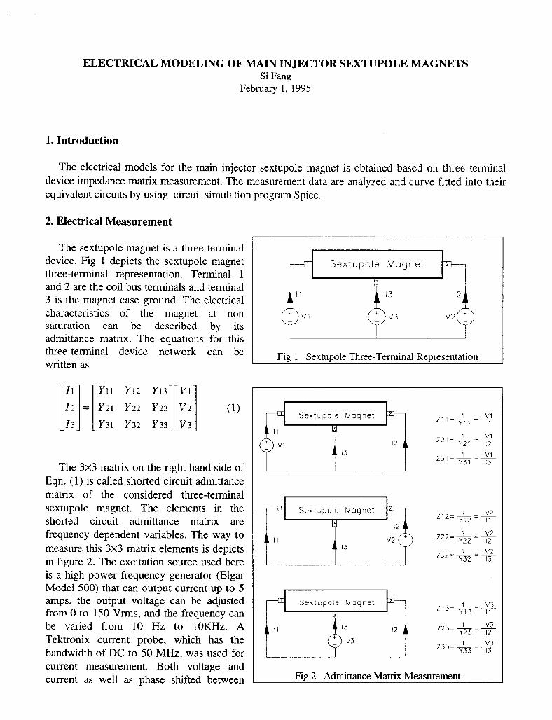
The sextupole magnet is a three-terminal device. Fig 1 depicts the sextupole magnet three-terminal representation. Terminal 1 and 2 are the coil bus terminals and terminal 3 is the magnet case ground. The electrical characteristics of the magnet at non saturation can be described by its admittance matrix. The equations for this
Sextupole Magnet
three-terminal device network can be written as
Fig 1 Sextupole Three-Terminal Representation
Yll Y12 Y13
Y21 Y22 Y23
Y31 Y32 Y33 I[ Vl
v2
v3 I (1)
The 3x3 matrix on the right hand side of Eqn. (1) is called shorted circuit admittance matrix of the considered three-terminal sextupole magnet. The elements in the shorted circuit admittance matrix are frequency dependent variables. The way to measure this 3x3 matrix elements is depicts in figure 2. The excitation source used here is a high power frequency generator (Elgar Model 500) that can output current up to 5 amps. the output voltage can be adjusted from 0 to 1.50 Vrms, and the frequency can be varied from 10 Hz to 1OKHz. A Tektronix current probe, which has the bandwidth of DC to 50 MHz, was used for current measurement. Both voltage and current as well as phase shifted between
1 v2 Z32= T37 = 13
Fig 2 Admittance Matrix Measurement

voltage and current were measured by Tektronix scope. Ratio of peak to peak value of current to voltage was obtained for the shorted circuit admittance at the frequency of interest. Scope measurement for voltage and current made sure the signals being measured were not distorted.
3. Measurement Data Fitting
DC Resistance of the coil bus is measured at 18 “C. The resistance then is scaled to the resistance at 40 “C by using the formula:
R(40”C)=R(18°C)~[1+0.004/o C(4O”C-18”C)] (2)
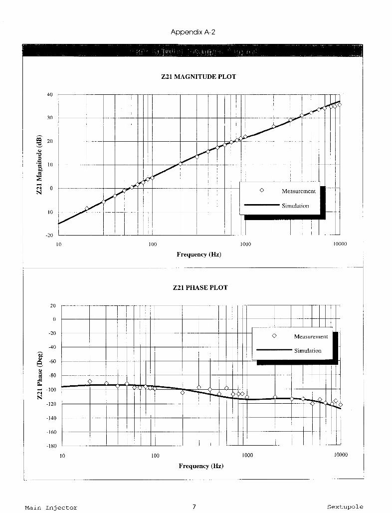
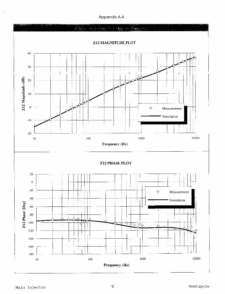
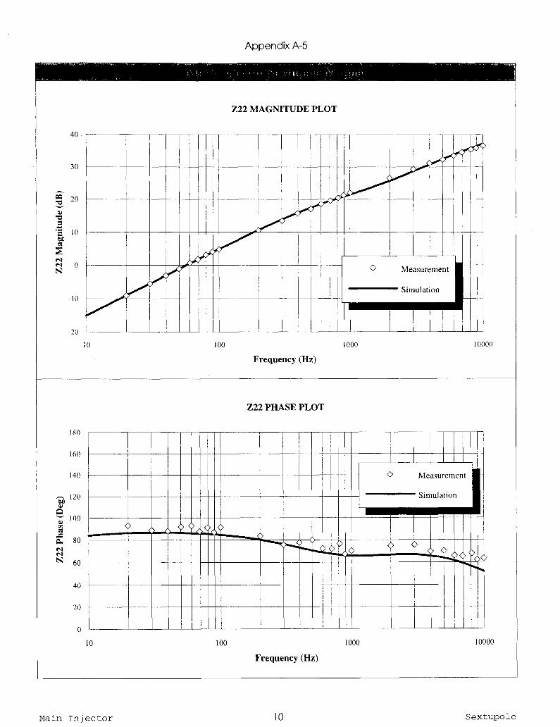
Coil Impedance measurement is performed by Zr 1, 222, 212, 221. ZI 1 and 222 are equal both in magnitude and phase for the frequency up to 10 KHz. 212 and 221 are also the same both in magnitude and phase. Zll and Z12 are the same in magnitude but 180” out of phase because the reverse direction of the current. This implies the Sextupole is symmetrical since impedance looking into both coil bus terminals is equal.
By analyzing the coil impedance measurement data Zlt and 222. The data can be represented by straight-line asymptotes as shown in Fig 3. The bus DC resistance has effect on coil impedance at very low frequency(c< 10 Hz), therefore it is not shown in the impedance asymptote representation here. The coil bus impedance is inductive at the frequency between 10 Hz and Fl , F2 and F3 because the slope of the magnitude asymptote line is 20 dB/decade and the phase is 90”. The coil bus becomes small resistive at the frequency between Fl and F2, and above F3. In the other word, the inductance of the coil decreases as the frequency increases.
A’ IZI dB
ZOdB/decade
F3
/
10 Frequency (Hz)
IOK
Fig 3 Coil Impedance Data Asymptote Representation
R3 R2
Rl I mLlr L2
w
Fl- ;i2 FZ=Ro F3-5
Z-T-L2 Z*Tr*Lo 2rnCLl
where Ll*L2 R2bR3 Lc=LltL2 R"=R2+R3
An electrical circuit shown in Fig 4 can be used to represent the straight-line asymptote characteristics in Fig 3. The L Fig 4 Circuit For Fig 3 Straight-Line Asymptote -- comer frequency break points are approximately given by the formula in figure 4.
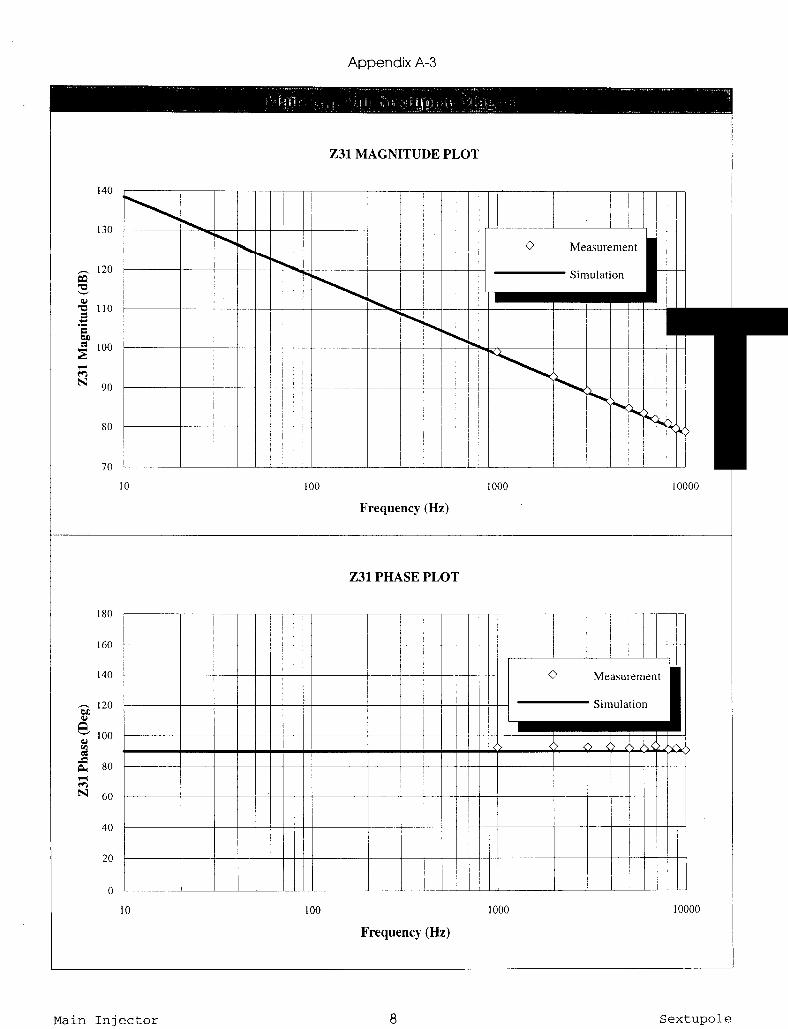
Bus Capacitance Measurement is obtained by 213, 231, 223, 232, and 233. 233 measures the total bus to ground capacitance. 213 and 231 measures the capacitance between terminal 1 and ground while
terminal 2 is shorted to ground. Similarly, 223 and 232 measures the capacitance between terminal 2
2
and ground while terminal 1 is grounded. The 213, 231, 223, 232, and 233 are capacitance measurement because the slope of the measurement data is -2OdB/decade in the magnitude plot. The capacitance is determined by the following formula
(3)
wherefis the excitation frequency in Hz and 2 is the impedance in ohms.
4. Sextupole Electrical Model
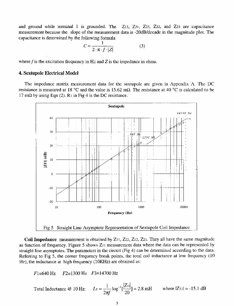
The impedance matrix measurement data for the sextupole are given in Appendix A. The DC resistance is measured at 18 “C and the value is 15.62 n-&J. The resistance at 40 “C is calculated to be 17 & by using Eqn (2). Rl in Fig 4 is the DC resistance.
Sextupole
14700 Hi!
10 100 1000 10000
Frequency (Hz)
Fig 5 Straight Line Asymptote Representation of Sextupole Coil Impedance
Coil Impedance measurement is obtained by Zt 1, 222, 212, 221. They all have the same magnitude as function of frequency. Figure 5 shows Zll measurement data where the data can be represented by straight line asymptotes. The parameters in the circuit (Fig 4) can be determined according to the data. Referring to Fig 5, the corner frequency break points, the total coil inductance at low frequency (10 Hz), the inductance at high frequency (1OKHz) are obtained as:
F1=640 Hz F2=1300 Hz F3=14700 Hz
Total Inductance @ 10 Hz: LT= 1 I I -log-l[~] = 2.8 mH where lZlll= -15.1 dB
Wf
3
Inductance @ 5 KHz: LI = J- log-’ [- I I 211
I = 1*3 mH where IZlll= 32.2 dB
2M 20
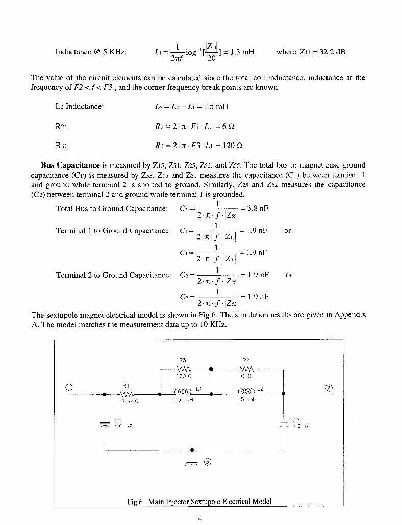
The value of the circuit elements can be calculated since the total coil inductance, inductance at the frequency of F2 c f < F3 , and the corner frequency break points are known.
L2 Inductance: L2= LT--1 = 1.5 Id3
R2: R2=2.n.Fl-L2 =6Q
R3: R4=2.n:-F3.L1 = 120R
Bus Capacitance is measured by Zts, Zst, 225, 252, and Zss. The total bus to magnet case ground capacitance (CT) is measured by Z55. Z15 and Z51 measures the capacitance (Cl) between terminal 1 and ground while terminal 2 is shorted to ground. Similarly, 225 and 252 measures the capacitance (0) between terminal 2 and ground while terminal 1 is grounded.
Total Bus to Ground Capacitance: 1
cT = 2. x. f . pssj = 3.8 nF
Terminal 1 to Ground Capacitance: CI = 1
2.n.f ./q = lo9 nF Or
1 c1= 2.7c.f.p5,1 = 1-9nF
Terminal 2 to Ground Capacitance: C2 = 1
2.n.f +4 = la9 nF Or
1 c2 = 2. x. f . lzs21 = la9 nF
The sextupole magnet electrical model is shown in Fig 6. The simulation results are given in Appendix A. The model matches the measurement data up to 10 KHz.
R3 R2 1 w
120 n 61-i
0 Rl pp)q-) Ll m LZ 0 I - a . . 17 rnn 1.3 mH 1.5 mH
Fig 6 Main Injector Sextupole Electrical Model
4

5. Conclusion
The sextupole electrical model is obtained based on the impedance matrix measurement. Spice simulation result shows the accuracy of the models. The electrical model can be used as a sub circuit to build a sextupole ring model to study the transient and frequency response of the system.
5
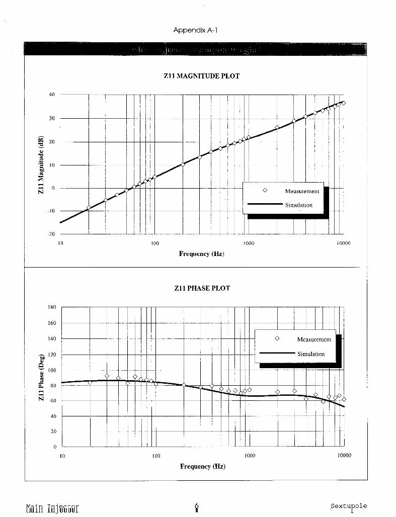
Appendix A- 1
Zll MAGNITUDE PLOT
30
-10
I
100
Frequency (Hz)
Measurement
180
140
8 120
5
s
100
e 80
z N 60
40
20
100
Zll PHASE PLOT
0 Measurement
Simulation
1000
Frequency (Hz)
Main Inj mar Q Sextupole
Appendix A-2
221 MAGNITUDE PLOT
40
30
s a *O
s -2 10
F E
74 0 N
-10
-20
Measurement -
7 10
Frequency (Hz)
221 PHASE PLOT
-20 Measurement
-40
% e
-60
Frequency (Hz)
7 Sextupole Main Injector
Appendix A-3
231 MAGNITUDE PLOT
r 130
0 Measurement
Simulation I:
s 120
5 110
.Z % m E 100
3 90
: I c 80
-1 70
Frequency (Hz)
1000 10000
231 PHASE PLOT
180
0 Measurement
160
140 j ! Simulation
I I I III/- I
G 120
a" - 100
s 2 80
;;: N 60
9
L
40
20
0
Frequency (Hz)
Main Injector 8 Sextupole
Appendix A-4
212 MAGNITUDE PLOT
40
30
g 20
s *z 10
z E
$1 0 N
-10
-20
I-
7F 10
Frequency (Hz)
-20
-40
9 e -60
: -80
2 2 -100
N -120
-140
-160
212 PHASE PLOT
Measurement
-180 i1 I I Illill I I Ill I I I I
10 100 1000
Frequency (Hz)
Main Injector 9 Sextupole
Appendix A-5
222 MAGNITUDE PLOT
40
30
RI
180
160
140
3 120
B - 100
s g 80
3 N 60
40
20
0
I- k c
-
-
-
-
-
/
-
-
L
Frequency (Hz)
222 PHASE PLOT
Measurement
100
Frequency (Hz)
1000 10000
Main Injector 10 Sextupole
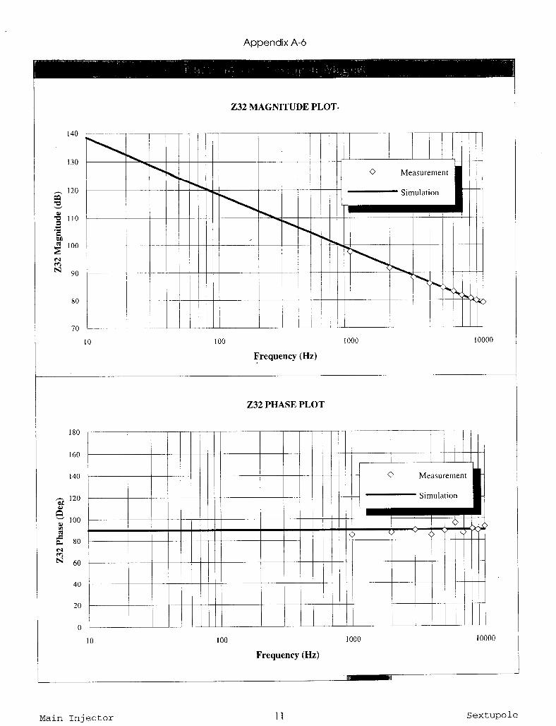
Appendix A-6
232 MAGNITUDE PLOT.
130
$ 110 .% Gl Q 100
E
80
Measurement
Frequency (Hz)
1000 10000
180
160
140
9 120
e
s
100
g 80
2 N 60
40
20
232 PHASE PLOT
Measurement
/ I I dli
100
Frequency (Hz)
1000 10000
Main Injector 11 Sextupole
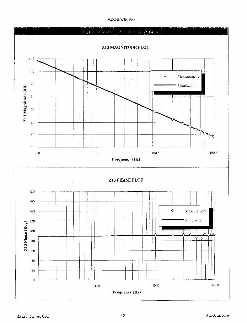
Appendix A-7
213 MAGNITUDE PLOT
140
130
3 120
$ 110
.Z
% m E 100
WI
z 90
80
70
10
c
c
I
r
I I I I
0 Measurement
Simulation / I
\ I P I I I I
\ ~I,1
I /
Frequency (Hz)
180
160
213 PHASE PLOT
Measureme
I? N 60
Frequency (Hz)
:nt
ilain Injector 12 Sextupole

Appendix A-8
223 MAGNITUDE PLOT
130
9
120
” 110
.%
5l m 100
E
a 90
80
70
0 Measurement
c
Frequency (Hz)
180
160
140
,--& 120
g 100
ii f 80
40
223 PHASE PLOT
Measurement
10
Frequency (Hz)
Main Injector 13 Sextupole
Top Related