


Languages
Pages
Legal


Title
regress postestimation — Postestimation tools for regress
Description
The following postestimation commands are of special interest after regress:
command description
dfbeta DFBETA influence statistics
estat hettest tests for heteroskedasticity
estat imtest information matrix test
estat ovtest Ramsey regression specification-error test for omitted variables
estat szroeter Szroeter’s rank test for heteroskedasticity
estat vif variance inflation factors for the independent variables
acprplot augmented component-plus-residual plot
avplot added-variable plot
avplots all added-variables plots in one image
cprplot component-plus-residual plot
lvr2plot leverage-versus-squared-residual plot
rvfplot residual-versus-fitted plot
rvpplot residual-versus-predictor plot
These commands are not appropriate after the svy prefix.
For information about these commands, see below.
1539
1540 regress postestimation — Postestimation tools for regress
The following standard postestimation commands are also available:
command description
estat AIC, BIC, VCE, and estimation sample summary
estat (svy) postestimation statistics for survey data
estimates cataloging estimation results
hausman Hausman’s specification test
lincom point estimates, standard errors, testing, and inference for linear combinationsof coefficients
linktest link test for model specification
lrtest1 likelihood-ratio test
margins marginal means, predictive margins, marginal effects, and average marginal effects
nlcom point estimates, standard errors, testing, and inference for nonlinearcombinations of coefficients
predict predictions, residuals, influence statistics, and other diagnostic measures
predictnl point estimates, standard errors, testing, and inference for generalizedpredictions
suest seemingly unrelated estimation
test Wald tests of simple and composite linear hypotheses
testnl Wald tests of nonlinear hypotheses
1 lrtest is not appropriate with svy estimation results.
See the corresponding entries in the Base Reference Manual for details, but see [SVY] estat for
details about estat (svy).
For postestimation tests specific to time series, see [R] regress postestimation time series.
Specialinterest postestimation commands
These commands provide tools for diagnosing sensitivity to individual observations, analyzingresiduals, and assessing specification.
dfbeta will calculate one, more than one, or all the DFBETAs after regress. Although predictwill also calculate DFBETAs, predict can do this for only one variable at a time. dfbeta is aconvenience tool for those who want to calculate DFBETAs for multiple variables. The names for thenew variables created are chosen automatically and begin with the letters dfbeta .
estat hettest performs three versions of the Breusch–Pagan (1979) and Cook–Weisberg (1983)test for heteroskedasticity. All three versions of this test present evidence against the null hypothesisthat t = 0 in Var(e) = σ2exp(zt). In the normal version, performed by default, the null hypothesisalso includes the assumption that the regression disturbances are independent-normal draws withvariance σ2. The normality assumption is dropped from the null hypothesis in the iid and fstatversions, which respectively produce the score and F tests discussed in Methods and formulas. Ifvarlist is not specified, the fitted values are used for z. If varlist or the rhs option is specified, thevariables specified are used for z.
estat imtest performs an information matrix test for the regression model and an orthogonal de-composition into tests for heteroskedasticity, skewness, and kurtosis due to Cameron and Trivedi (1990);White’s test for homoskedasticity against unrestricted forms of heteroskedasticity (1980) is availableas an option. White’s test is usually similar to the first term of the Cameron–Trivedi decomposition.

regress postestimation — Postestimation tools for regress 1541
estat ovtest performs two versions of the Ramsey (1969) regression specification-error test(RESET) for omitted variables. This test amounts to fitting y = xb + zt + u and then testing t = 0.If the rhs option is not specified, powers of the fitted values are used for z. If rhs is specified,powers of the individual elements of x are used.
estat szroeter performs Szroeter’s rank test for heteroskedasticity for each of the variables invarlist or for the explanatory variables of the regression if rhs is specified.
estat vif calculates the centered or uncentered variance inflation factors (VIFs) for the independentvariables specified in a linear regression model.
acprplot graphs an augmented component-plus-residual plot (a.k.a. augmented partial residualplot) as described by Mallows (1986). This seems to work better than the component-plus-residualplot for identifying nonlinearities in the data.
avplot graphs an added-variable plot (a.k.a. partial-regression leverage plot, partial regressionplot, or adjusted partial residual plot) after regress. indepvar may be an independent variable (a.k.a.predictor, carrier, or covariate) that is currently in the model or not.
avplots graphs all the added-variable plots in one image.
cprplot graphs a component-plus-residual plot (a.k.a. partial residual plot) after regress. indepvarmust be an independent variable that is currently in the model.
lvr2plot graphs a leverage-versus-squared-residual plot (a.k.a. L-R plot).
rvfplot graphs a residual-versus-fitted plot, a graph of the residuals against the fitted values.
rvpplot graphs a residual-versus-predictor plot (a.k.a. independent variable plot or carrier plot),a graph of the residuals against the specified predictor.
(Continued on next page)

1542 regress postestimation — Postestimation tools for regress
Syntax for predict
predict[type
]newvar
[if] [
in] [
, statistic]
statistic description
xb linear prediction; the default
residuals residuals
score score; equivalent to residuals
rstandard standardized residuals
rstudent studentized (jackknifed) residuals
cooksd Cook’s distance
leverage | hat leverage (diagonal elements of hat matrix)
pr(a,b) Pr(yj | a < yj < b)
e(a,b) E(yj | a < yj < b)
ystar(a,b) E(y∗j ), y∗j = max{a,min(yj , b)}∗dfbeta(varname) DFBETA for varname
stdp standard error of the linear prediction
stdf standard error of the forecast
stdr standard error of the residual∗covratio COVRATIO∗dfits DFITS∗welsch Welsch distance
Unstarred statistics are available both in and out of sample; type predict . . . if e(sample) . . . if wanted only forthe estimation sample. Starred statistics are calculated only for the estimation sample, even when if e(sample)is not specified.
rstandard, rstudent, cooksd, leverage, dfbeta(), stdf, stdr, covratio, dfits, and welsch are not availableif any vce() other than vce(ols) was specified with regress.
xb, residuals, score, and stdp are the only options allowed with svy estimation results.
where a and b may be numbers or variables; a missing (a ≥ .) means −∞, and b missing (b ≥ .) means +∞; see[U] 12.2.1 Missing values.
Menu
Statistics > Postestimation > Predictions, residuals, etc.
Options for predict
xb, the default, calculates the linear prediction.
residuals calculates the residuals.
score is equivalent to residuals in linear regression.
rstandard calculates the standardized residuals.
rstudent calculates the studentized (jackknifed) residuals.
cooksd calculates the Cook’s D influence statistic (Cook 1977).
leverage or hat calculates the diagonal elements of the projection hat matrix.
regress postestimation — Postestimation tools for regress 1543
pr(a,b) calculates Pr(a < xjb + uj < b), the probability that yj|xj would be observed in theinterval (a, b).
a and b may be specified as numbers or variable names; lb and ub are variable names;pr(20,30) calculates Pr(20 < xjb + uj < 30);pr(lb,ub) calculates Pr(lb < xjb + uj < ub);and pr(20,ub) calculates Pr(20 < xjb + uj < ub).
a missing (a ≥ .) means −∞; pr(.,30) calculates Pr(−∞ < xjb + uj < 30);pr(lb,30) calculates Pr(−∞ < xjb + uj < 30) in observations for which lb ≥ .and calculates Pr(lb < xjb + uj < 30) elsewhere.
b missing (b ≥ .) means +∞; pr(20,.) calculates Pr(+∞ > xjb + uj > 20);pr(20,ub) calculates Pr(+∞ > xjb + uj > 20) in observations for which ub ≥ .and calculates Pr(20 < xjb + uj < ub) elsewhere.
e(a,b) calculates E(xjb + uj | a < xjb + uj < b), the expected value of yj |xj conditional onyj|xj being in the interval (a, b), meaning that yj |xj is censored.a and b are specified as they are for pr().
ystar(a,b) calculates E(y∗j ), where y∗j = a if xjb + uj ≤ a, y∗j = b if xjb + uj ≥ b, andy∗j = xjb + uj otherwise, meaning that y∗j is truncated. a and b are specified as they are forpr().
dfbeta(varname) calculates the DFBETA for varname, the difference between the regression coefficientwhen the jth observation is included and excluded, said difference being scaled by the estimatedstandard error of the coefficient. varname must have been included among the regressors in thepreviously fitted model. The calculation is automatically restricted to the estimation subsample.
stdp calculates the standard error of the prediction, which can be thought of as the standard error ofthe predicted expected value or mean for the observation’s covariate pattern. The standard errorof the prediction is also referred to as the standard error of the fitted value.
stdf calculates the standard error of the forecast, which is the standard error of the point predictionfor 1 observation. It is commonly referred to as the standard error of the future or forecast value.By construction, the standard errors produced by stdf are always larger than those produced bystdp; see Methods and formulas.
stdr calculates the standard error of the residuals.
covratio calculates COVRATIO (Belsley, Kuh, and Welsch 1980), a measure of the influence of thejth observation based on considering the effect on the variance–covariance matrix of the estimates.The calculation is automatically restricted to the estimation subsample.
dfits calculates DFITS (Welsch and Kuh 1977) and attempts to summarize the information in theleverage versus residual-squared plot into one statistic. The calculation is automatically restrictedto the estimation subsample.
welsch calculates Welsch distance (Welsch 1982) and is a variation on dfits. The calculation isautomatically restricted to the estimation subsample.
Syntax for dfbeta
dfbeta[indepvar
[indepvar
[. . .] ] ] [
, stub(name)]

1544 regress postestimation — Postestimation tools for regress
Menu
Statistics > Linear models and related > Regression diagnostics > Residual-versus-fitted plot
Option for dfbeta
stub(name) specifies the leading characters dfbeta uses to name the new variables to be generated.The default is stub( dfbeta ).
Syntax for estat hettest
estat hettest[varlist
] [, rhs
[normal | iid | fstat
]mtest
[(spec)
] ]
Menu
Statistics > Postestimation > Reports and statistics
Options for estat hettest
rhs specifies that tests for heteroskedasticity be performed for the right-hand-side (explanatory)variables of the fitted regression model. The rhs option may be combined with a varlist.
normal, the default, causes estat hettest to compute the original Breusch–Pagan/Cook–Weisbergtest, which assumes that the regression disturbances are normally distributed.
iid causes estat hettest to compute the N ∗R2 version of the score test that drops the normalityassumption.
fstat causes estat hettest to compute the F statistic version that drops the normality assumption.
mtest[(spec)
]specifies that multiple testing be performed. The argument specifies how p-values
are adjusted. The following specifications, spec, are supported:
bonferroni Bonferroni’s multiple testing adjustmentholm Holm’s multiple testing adjustmentsidak Sidak’s multiple testing adjustment
noadjust no adjustment is made for multiple testing
mtest may be specified without an argument. This is equivalent to specifying mtest(noadjust),that is, tests for the individual variables should be performed with unadjusted p-values. By default,estat hettest does not perform multiple testing. mtest
[(spec)
]may not be specified with
iid or fstat.
Syntax for estat imtest
estat imtest[, preserve white
]

regress postestimation — Postestimation tools for regress 1545
MenuStatistics > Postestimation > Reports and statistics
Options for estat imtest
preserve specifies that the data in memory be preserved, all variables and cases that are not neededin the calculations be dropped, and at the conclusion the original data be restored. This option iscostly for large datasets. However, because estat imtest has to perform an auxiliary regressionon k(k + 1)/2 temporary variables, where k is the number of regressors, it may not be able toperform the test otherwise.
white specifies that White’s original heteroskedasticity test also be performed.
Syntax for estat ovtest
estat ovtest[, rhs
]
MenuStatistics > Postestimation > Reports and statistics
Option for estat ovtest
rhs specifies that powers of the right-hand-side (explanatory) variables be used in the test rather thanpowers of the fitted values.
Syntax for estat szroeter
estat szroeter[varlist
] [, rhs mtest(spec)
]
Either varlist or rhs must be specified.
Menu
Statistics > Postestimation > Reports and statistics
Options for estat szroeter
rhs specifies that tests for heteroskedasticity be performed for the right-hand-side (explanatory)variables of the fitted regression model. Option rhs may be combined with a varlist.
mtest(spec) specifies that multiple testing be performed. The argument specifies how p-values areadjusted. The following specifications spec are supported:
bonferroni Bonferroni’s multiple testing adjustmentholm Holm’s multiple testing adjustmentsidak Sidak’s multiple testing adjustment
noadjust no adjustment is made for multiple testing

1546 regress postestimation — Postestimation tools for regress
estat szroeter always performs multiple testing. By default, it does not adjust the p-values.
Syntax for estat vif
estat vif[, uncentered
]
Menu
Statistics > Postestimation > Reports and statistics
Option for estat vif
uncentered requests that the computation of the uncentered variance inflation factors. This option isoften used to detect the collinearity of the regressors with the constant. estat vif, uncentered
may be used after regression models fit without the constant term.
Syntax for acprplot
acprplot indepvar[, acprplot options
]
acprplot options description
Plot
marker options change look of markers (color, size, etc.)
marker label options add marker labels; change look or position
Reference line
rlopts(cline options) affect rendition of the reference line
Options
lowess add a lowess smooth of the plotted points
lsopts(lowess options) affect rendition of the lowess smooth
mspline add median spline of the plotted points
msopts(mspline options) affect rendition of the spline
Add plots
addplot(plot) add other plots to the generated graph
Y axis, X axis, Titles, Legend, Overall
twoway options any options other than by() documented in [G] twoway options
Menu
Statistics > Linear models and related > Regression diagnostics > Augmented component-plus-residual plot

regress postestimation — Postestimation tools for regress 1547
Options for acprplot
�
� �
Plot �
marker options affect the rendition of markers drawn at the plotted points, including their shape,size, color, and outline; see [G] marker options.
marker label options specify if and how the markers are to be labeled; see [G] marker label options.
�
� �
Reference line �
rlopts(cline options) affects the rendition of the reference line. See [G] cline options.
�
� �
Options �
lowess adds a lowess smooth of the plotted points to assist in detecting nonlinearities.
lsopts(lowess options) affects the rendition of the lowess smooth. For an explanation of theseoptions, especially the bwidth() option, see [R] lowess. Specifying lsopts() implies the lowessoption.
mspline adds a median spline of the plotted points to assist in detecting nonlinearities.
msopts(mspline options) affects the rendition of the spline. For an explanation of these options,especially the bands() option, see [G] graph twoway mspline. Specifying msopts() implies themspline option.
�
� �
Add plots �
addplot(plot) provides a way to add other plots to the generated graph. See [G] addplot option.
�
� �
Y axis, X axis, Titles, Legend, Overall �
twoway options are any of the options documented in [G] twoway options, excluding by(). Theseinclude options for titling the graph (see [G] title options) and for saving the graph to disk (see[G] saving option).
Syntax for avplot
avplot indepvar[, avplot options
]
avplot options description
Plot
marker options change look of markers (color, size, etc.)
marker label options add marker labels; change look or position
Reference line
rlopts(cline options) affect rendition of the reference line
Add plots
addplot(plot) add other plots to the generated graph
Y axis, X axis, Titles, Legend, Overall
twoway options any options other than by() documented in [G] twoway options

1548 regress postestimation — Postestimation tools for regress
Menu
Statistics > Linear models and related > Regression diagnostics > Added-variable plot
Options for avplot
�
� �
Plot �
marker options affect the rendition of markers drawn at the plotted points, including their shape,size, color, and outline; see [G] marker options.
marker label options specify if and how the markers are to be labeled; see [G] marker label options.
�
� �
Reference line �
rlopts(cline options) affects the rendition of the reference line. See [G] cline options.
�
� �
Add plots �
addplot(plot) provides a way to add other plots to the generated graph. See [G] addplot option.
�
� �
Y axis, X axis, Titles, Legend, Overall �
twoway options are any of the options documented in [G] twoway options, excluding by(). Theseinclude options for titling the graph (see [G] title options) and for saving the graph to disk (see[G] saving option).
Syntax for avplots
avplots[, avplots options
]
avplots options description
Plot
marker options change look of markers (color, size, etc.)
marker label options add marker labels; change look or position
combine options any of the options documented in [G] graph combine
Reference line
rlopts(cline options) affect rendition of the reference line
Y axis, X axis, Titles, Legend, Overall
twoway options any options other than by() documented in [G] twoway options
Menu
Statistics > Linear models and related > Regression diagnostics > Added-variable plot

regress postestimation — Postestimation tools for regress 1549
Options for avplots
�
� �
Plot �
marker options affect the rendition of markers drawn at the plotted points, including their shape,size, color, and outline; see [G] marker options.
marker label options specify if and how the markers are to be labeled; see [G] marker label options.
combine options are any of the options documented in [G] graph combine. These include options fortitling the graph (see [G] title options) and for saving the graph to disk (see [G] saving option).
�
� �
Reference line �
rlopts(cline options) affects the rendition of the reference line. See [G] cline options.
�
� �
Y axis, X axis, Titles, Legend, Overall �
twoway options are any of the options documented in [G] twoway options, excluding by(). Theseinclude options for titling the graph (see [G] title options) and for saving the graph to disk (see[G] saving option).
Syntax for cprplot
cprplot indepvar[, cprplot options
]
cprplot options description
Plot
marker options change look of markers (color, size, etc.)
marker label options add marker labels; change look or position
Reference line
rlopts(cline options) affect rendition of the reference line
Options
lowess add a lowess smooth of the plotted points
lsopts(lowess options) affect rendition of the lowess smooth
mspline add median spline of the plotted points
msopts(mspline options) affect rendition of the spline
Add plots
addplot(plot) add other plots to the generated graph
Y axis, X axis, Titles, Legend, Overall
twoway options any options other than by() documented in [G] twoway options
Menu
Statistics > Linear models and related > Regression diagnostics > Component-plus-residual plot

1550 regress postestimation — Postestimation tools for regress
Options for cprplot
�
� �
Plot �
marker options affect the rendition of markers drawn at the plotted points, including their shape,size, color, and outline; see [G] marker options.
marker label options specify if and how the markers are to be labeled; see [G] marker label options.
�
� �
Reference line �
rlopts(cline options) affects the rendition of the reference line. See [G] cline options.
�
� �
Options �
lowess adds a lowess smooth of the plotted points to assist in detecting nonlinearities.
lsopts(lowess options) affects the rendition of the lowess smooth. For an explanation of theseoptions, especially the bwidth() option, see [R] lowess. Specifying lsopts() implies the lowessoption.
mspline adds a median spline of the plotted points to assist in detecting nonlinearities.
msopts(mspline options) affects the rendition of the spline. For an explanation of these options,especially the bands() option, see [G] graph twoway mspline. Specifying msopts() implies themspline option.
�
� �
Add plots �
addplot(plot) provides a way to add other plots to the generated graph. See [G] addplot option.
�
� �
Y axis, X axis, Titles, Legend, Overall �
twoway options are any of the options documented in [G] twoway options, excluding by(). Theseinclude options for titling the graph (see [G] title options) and for saving the graph to disk (see[G] saving option).
Syntax for lvr2plot
lvr2plot[, lvr2plot options
]
lvr2plot options description
Plot
marker options change look of markers (color, size, etc.)
marker label options add marker labels; change look or position
Add plots
addplot(plot) add other plots to the generated graph
Y axis, X axis, Titles, Legend, Overall
twoway options any options other than by() documented in [G] twoway options

regress postestimation — Postestimation tools for regress 1551
Menu
Statistics > Linear models and related > Regression diagnostics > Leverage-versus-squared-residual plot
Options for lvr2plot
�
� �
Plot �
marker options affect the rendition of markers drawn at the plotted points, including their shape,size, color, and outline; see [G] marker options.
marker label options specify if and how the markers are to be labeled; see [G] marker label options.
�
� �
Add plots �
addplot(plot) provides a way to add other plots to the generated graph; see [G] addplot option.
�
� �
Y axis, X axis, Titles, Legend, Overall �
twoway options are any of the options documented in [G] twoway options, excluding by(). Theseinclude options for titling the graph (see [G] title options) and for saving the graph to disk (see[G] saving option).
Syntax for rvfplot
rvfplot[, rvfplot options
]
rvfplot options description
Plot
marker options change look of markers (color, size, etc.)
marker label options add marker labels; change look or position
Add plots
addplot(plot) add plots to the generated graph
Y axis, X axis, Titles, Legend, Overall
twoway options any options other than by() documented in [G] twoway options
Menu
Statistics > Linear models and related > Regression diagnostics > Residual-versus-fitted plot
Options for rvfplot
�
� �
Plot �
marker options affect the rendition of markers drawn at the plotted points, including their shape,size, color, and outline; see [G] marker options.
marker label options specify if and how the markers are to be labeled; see [G] marker label options.

1552 regress postestimation — Postestimation tools for regress
�
� �
Add plots �
addplot(plot) provides a way to add plots to the generated graph. See [G] addplot option.
�
� �
Y axis, X axis, Titles, Legend, Overall �
twoway options are any of the options documented in [G] twoway options, excluding by(). Theseinclude options for titling the graph (see [G] title options) and for saving the graph to disk (see[G] saving option).
Syntax for rvpplot
rvpplot indepvar[, rvpplot options
]
rvpplot options description
Plot
marker options change look of markers (color, size, etc.)
marker label options add marker labels; change look or position
Add plots
addplot(plot) add other plots to the generated graph
Y axis, X axis, Titles, Legend, Overall
twoway options any options other than by() documented in [G] twoway options
Menu
Statistics > Linear models and related > Regression diagnostics > Residual-versus-predictor plot
Options for rvpplot
�
� �
Plot �
marker options affect the rendition of markers drawn at the plotted points, including their shape,size, color, and outline; see [G] marker options.
marker label options specify if and how the markers are to be labeled; see [G] marker label options.
�
� �
Add plots �
addplot(plot) provides a way to add other plots to the generated graph; see [G] addplot option.
�
� �
Y axis, X axis, Titles, Legend, Overall �
twoway options are any of the options documented in [G] twoway options, excluding by(). Theseinclude options for titling the graph (see [G] title options) and for saving the graph to disk (see[G] saving option).

regress postestimation — Postestimation tools for regress 1553
Remarks
Remarks are presented under the following headings:
Fitted values and residualsPrediction standard errorsPrediction with weighted dataResidual-versus-fitted plotsAdded-variable plotsComponent-plus-residual plotsResidual-versus-predictor plotsLeverage statisticsL-R plotsStandardized and studentized residualsDFITS, Cook’s Distance, and Welsch DistanceCOVRATIODFBETAsFormal tests for violations of assumptionsVariance inflation factors
Many of these commands concern identifying influential data in linear regression. This is, un-fortunately, a field that is dominated by jargon, codified and partially begun by Belsley, Kuh, andWelsch (1980). In the words of Chatterjee and Hadi (1986, 416), “Belsley, Kuh, and Welsch’s book,Regression Diagnostics, was a very valuable contribution to the statistical literature, but it unleashedon an unsuspecting statistical community a computer speak (a la Orwell), the likes of which wehave never seen.” Things have only gotten worse since then. Chatterjee and Hadi’s (1986, 1988)own attempts to clean up the jargon did not improve matters (see Hoaglin and Kempthorne [1986],Velleman [1986], and Welsch [1986]). We apologize for the jargon, and for our contribution to thejargon in the form of inelegant command names, we apologize most of all.
Model sensitivity refers to how estimates are affected by subsets of our data. Imagine data on yand x, and assume that the data are to be fit by the regression yi = α + βxi + ǫi. The regressionestimates of α and β are a and b, respectively. Now imagine that the estimated a and b would bedifferent if a small portion of the dataset, perhaps even one observation, were deleted. As a dataanalyst, you would like to think that you are summarizing tendencies that apply to all the data, butyou have just been told that the model you fit is unduly influenced by one point or just a few pointsand that, as a matter of fact, there is another model that applies to the rest of the data—a modelthat you have ignored. The search for subsets of the data that, if deleted, would change the resultsmarkedly is a predominant theme of this entry.
There are three key issues in identifying model sensitivity to individual observations, which go bythe names residuals, leverage, and influence. In our yi = a+ bxi + ei regression, the residuals are,of course, ei—they reveal how much our fitted value yi = a+ bxi differs from the observed yi. Apoint (xi, yi) with a corresponding large residual is called an outlier. Say that you are interested inoutliers because you somehow think that such points will exert undue influence on your estimates.Your feelings are generally right, but there are exceptions. A point might have a huge residual andyet not affect the estimated b at all. Nevertheless, studying observations with large residuals almostalways pays off.
(xi, yi) can be an outlier in another way—just as yi can be far from yi, xi can be far fromthe center of mass of the other x’s. Such an “outlier” should interest you just as much as the moretraditional outliers. Picture a scatterplot of y against x with thousands of points in some sort of massat the lower left of the graph and one point at the upper right of the graph. Now run a regressionline through the points—the regression line will come close to the point at the upper right of thegraph and may in fact, go through it. That is, this isolated point will not appear as an outlier asmeasured by residuals because its residual will be small. Yet this point might have a dramatic effecton our resulting estimates in the sense that, were you to delete the point, the estimates would change

1554 regress postestimation — Postestimation tools for regress
markedly. Such a point is said to have high leverage. Just as with traditional outliers, a high leveragepoint does not necessarily have an undue effect on regression estimates, but if it does not, it is morethe exception than the rule.
Now all this is a most unsatisfactory state of affairs. Points with large residuals may, but neednot, have a large effect on our results, and points with small residuals may still have a large effect.Points with high leverage may, but need not, have a large effect on our results, and points with lowleverage may still have a large effect. Can you not identify the influential points and simply have thecomputer list them for you? You can, but you will have to define what you mean by “influential”.
“Influential” is defined with respect to some statistic. For instance, you might ask which points inyour data have a large effect on your estimated a, which points have a large effect on your estimatedb, which points have a large effect on your estimated standard error of b, and so on, but do not besurprised when the answers to these questions are different. In any case, obtaining such measuresis not difficult—all you have to do is fit the regression excluding each observation one at a timeand record the statistic of interest which, in the day of the modern computer, is not too onerous.Moreover, you can save considerable computer time by doing algebra ahead of time and workingout formulas that will calculate the same answers as if you ran each of the regressions. (Ignore thequestion of pairs of observations that, together, exert undue influence, and triples, and so on, whichremains largely unsolved and for which the brute force fit-every-possible-regression procedure is nota viable alternative.)
Fitted values and residuals
Typing predict newvar with no options creates newvar containing the fitted values. Typingpredict newvar, resid creates newvar containing the residuals.
Example 1
Continuing with example 1 from [R] regress, we wish to fit the following model:
mpg = β0 + β1weight + β2weight2 + β3foreign + ǫ
. use http://www.stata-press.com/data/r11/auto(1978 Automobile Data)
. regress mpg weight c.weight#c.weight foreign
Source SS df MS Number of obs = 74F( 3, 70) = 52.25
Model 1689.15372 3 563.05124 Prob > F = 0.0000Residual 754.30574 70 10.7757963 R-squared = 0.6913
Adj R-squared = 0.6781Total 2443.45946 73 33.4720474 Root MSE = 3.2827
mpg Coef. Std. Err. t P>|t| [95% Conf. Interval]
weight -.0165729 .0039692 -4.18 0.000 -.0244892 -.0086567
c.weight#c.weight 1.59e-06 6.25e-07 2.55 0.013 3.45e-07 2.84e-06
foreign -2.2035 1.059246 -2.08 0.041 -4.3161 -.0909002_cons 56.53884 6.197383 9.12 0.000 44.17855 68.89913

regress postestimation — Postestimation tools for regress 1555
That done, we can now obtain the predicted values from the regression. We will store them in a newvariable called pmpg by typing predict pmpg. Because predict produces no output, we will followthat by summarizing our predicted and observed values.
. predict pmpg(option xb assumed; fitted values)
. summarize pmpg mpg
Variable Obs Mean Std. Dev. Min Max
pmpg 74 21.2973 4.810311 13.59953 31.86288mpg 74 21.2973 5.785503 12 41
Example 2: Out-of-sample predictions
We can just as easily obtain predicted values from the model by using a wholly different datasetfrom the one on which the model was fit. The only requirement is that the data have the necessaryvariables, which here are weight and foreign.
Using the data on two new cars (the Pontiac Sunbird and the Volvo 260) from the newautos.dtadataset, we can obtain out-of-sample predictions (or forecasts) by typing
. use http://www.stata-press.com/data/r11/newautos, clear(New Automobile Models)
. predict pmpg(option xb assumed; fitted values)
. list, divider
make weight foreign pmpg
1. Pont. Sunbird 2690 Domestic 23.471372. Volvo 260 3170 Foreign 17.78846
The Pontiac Sunbird has a predicted mileage rating of 23.5 mpg, whereas the Volvo 260 has apredicted rating of 17.8 mpg. In comparison, the actual mileage ratings are 24 for the Pontiac and17 for the Volvo.
Prediction standard errors
predict can calculate the standard error of the forecast (stdf option), the standard error of theprediction (stdp option), and the standard error of the residual (stdr option). It is easy to confusestdf and stdp because both are often called the prediction error. Consider the prediction yj = xjb,where b is the estimated coefficient (column) vector and xj is a (row) vector of independent variablesfor which you want the prediction. First, yj has a variance due to the variance of the estimatedcoefficient vector b,
Var(yj) = Var(xjb) = s2hj
where hj = xj(X′X)−1x′
j and s2 is the mean squared error of the regression. Do not panic over the
algebra—just remember that Var(yj) = s2hj , whatever s2 and hj are. stdp calculates this quantity.
This is the error in the prediction due to the uncertainty about b.

1556 regress postestimation — Postestimation tools for regress
If you are about to hand this number out as your forecast, however, there is another error. Accordingto your model, the true value of yj is given by
yj = xjb + ǫj = yj + ǫj
and thus the Var(yj) = Var(yj) + Var(ǫj) = s2hj + s2, which is the square of stdf. stdf, then,is the sum of the error in the prediction plus the residual error.
stdr has to do with an analysis-of-variance decomposition of s2, the estimated variance of y.The standard error of the prediction is s2hj , and therefore s2hj + s2(1− hj) = s2 decomposes s2
into the prediction and residual variances.
Example 3: standard error of the forecast
Returning to our model of mpg on weight, weight2 , and foreign, we previously predicted themileage rating for the Pontiac Sunbird and Volvo 260 as 23.5 and 17.8 mpg, respectively. We nowwant to put a standard error around our forecast. Remember, the data for these two cars were innewautos.dta:
. use http://www.stata-press.com/data/r11/newautos, clear(New Automobile Models)
. predict pmpg(option xb assumed; fitted values)
. predict se_pmpg, stdf
. list, divider
make weight foreign pmpg se_pmpg
1. Pont. Sunbird 2690 Domestic 23.47137 3.3418232. Volvo 260 3170 Foreign 17.78846 3.438714
Thus an approximate 95% confidence interval for the mileage rating of the Volvo 260 is 17.8±2·3.44 =[ 10.92, 24.68 ].
Prediction with weighted data
predict can be used after frequency-weighted (fweight) estimation, just as it is used afterunweighted estimation. The technical note below concerns the use of predict after analyticallyweighted (aweight) estimation.
Technical note
After analytically weighted estimation, predict is willing to calculate only the prediction (nooptions), residual (residual option), standard error of the prediction (stdp option), and diagonalelements of the projection matrix (hat option). Moreover, the results produced by hat need tobe adjusted, as will be described. For analytically weighted estimation, the standard error of theforecast and residuals, the standardized and studentized residuals, and Cook’s D are not statisticallywell-defined concepts.
To obtain the correct values of the diagonal elements of the hat matrix, you can use predictwith the hat option to make a first, partially adjusted calculation, and then follow that by completingthe adjustment. Assume that you are fitting a linear regression model weighting the data with thevariable w ([aweight=w]). Begin by creating a new variable, w0:

regress postestimation — Postestimation tools for regress 1557
. predict resid if e(sample), resid
. summarize w if resid < . & e(sample)
. gen w0=w/r(mean)
Some caution is necessary at this step—the summarize w must be performed on the same sample thatwas used to fit the model, which means that you must include if e(sample) to restrict the predictionto the estimation sample. You created the residual and then included the modifier ‘if resid < .’so that if the dependent variable or any of the independent variables is missing, the correspondingobservations will be excluded from the calculation of the average value of the original weight.
To correct predict’s hat calculation, multiply the result by w0:
. predict myhat, hat
. replace myhat = w0 * myhat
Residualversusfitted plots
Example 4: rvfplot
Using the automobile dataset described in [U] 1.2.2 Example datasets, we will use regress to fita model of price on weight, mpg, foreign, and the interaction of foreign with mpg. We specifyforeign##c.mpg to obtain the interaction of foreign with mpg; see [U] 11.4.3 Factor variables.
. use http://www.stata-press.com/data/r11/auto, clear(1978 Automobile Data)
. regress price weight foreign##c.mpg
Source SS df MS Number of obs = 74F( 4, 69) = 21.22
Model 350319665 4 87579916.3 Prob > F = 0.0000Residual 284745731 69 4126749.72 R-squared = 0.5516
Adj R-squared = 0.5256Total 635065396 73 8699525.97 Root MSE = 2031.4
price Coef. Std. Err. t P>|t| [95% Conf. Interval]
weight 4.613589 .7254961 6.36 0.000 3.166263 6.0609141.foreign 11240.33 2751.681 4.08 0.000 5750.878 16729.78
mpg 263.1875 110.7961 2.38 0.020 42.15527 484.2197
foreign#c.mpg
1 -307.2166 108.5307 -2.83 0.006 -523.7294 -90.70368
_cons -14449.58 4425.72 -3.26 0.002 -23278.65 -5620.51
Once we have fit a model, we may use any of the regression diagnostics commands. rvfplot(read residual-versus-fitted plot) graphs the residuals against the fitted values:

1558 regress postestimation — Postestimation tools for regress
. rvfplot, yline(0)
−50
00
05000
10000
Resid
uals
2000 4000 6000 8000 10000 12000Fitted values
All the diagnostic plot commands allow the graph twoway and graph twoway scatter options;we specified a yline(0) to draw a line across the graph at y = 0; see [G] graph twoway scatter.
In a well-fitted model, there should be no pattern to the residuals plotted against the fittedvalues—something not true of our model. Ignoring the two outliers at the top center of the graph,we see curvature in the pattern of the residuals, suggesting a violation of the assumption that priceis linear in our independent variables. We might also have seen increasing or decreasing variation inthe residuals—heteroskedasticity. Any pattern whatsoever indicates a violation of the least-squaresassumptions.
Addedvariable plots
Example 5: avplot
We continue with our price model, and another diagnostic graph is provided by avplot (readadded-variable plot, also known as the partial-regression leverage plot).
One of the wonderful features of one-regressor regressions (regressions of y on one x) is that wecan graph the data and the regression line. There is no easier way to understand the regression thanto examine such a graph. Unfortunately, we cannot do this when we have more than one regressor.With two regressors, it is still theoretically possible—the graph must be drawn in three dimensions,but with three or more regressors no graph is possible.
The added-variable plot is an attempt to project multidimensional data back to the two-dimensionalworld for each of the original regressors. This is, of course, impossible without making someconcessions. Call the coordinates on an added-variable plot y and x. The added-variable plot has thefollowing properties:
• There is a one-to-one correspondence between (xi, yi) and the ith observation used in the originalregression.
• A regression of y on x has the same coefficient and standard error (up to a degree-of-freedomadjustment) as the estimated coefficient and standard error for the regressor in the original regression.

regress postestimation — Postestimation tools for regress 1559
• The “outlierness” of each observation in determining the slope is in some sense preserved.
It is equally important to note the properties that are not listed. The y and x coordinates of theadded-variable plot cannot be used to identify functional form, or, at least, not well (see Mallows[1986]). In the construction of the added-variable plot, the relationship between y and x is forced tobe linear.
Let’s examine the added-variable plot for mpg in our regression of price on weight andforeign##c.mpg:
. avplot mpg
−4000
−2000
02000
4000
6000
e(
price | X
)
−5 0 5 10e( mpg | X )
coef = 263.18749, se = 110.79612, t = 2.38
This graph suggests a problem in determining the coefficient on mpg. Were this a one-regressorregression, the two points at the top-left corner and the one at the top right would cause us concern,and so it does in our more complicated multiple-regressor case. To identify the problem points, weretyped our command, modifying it to read avplot mpg, mlabel(make), and discovered that thetwo cars at the top left are the Cadillac Eldorado and the Lincoln Versailles; the point at the top rightis the Cadillac Seville. These three cars account for 100% of the luxury cars in our data, suggestingthat our model is misspecified. By the way, the point at the lower right of the graph, also cause forconcern, is the Plymouth Arrow, our data-entry error.
Technical note
Stata’s avplot command can be used with regressors already in the model, as we just did, orwith potential regressors not yet in the model. In either case, avplot will produce the correct graph.The name “added-variable plot” is unfortunate in the case when the variable is already among the listof regressors but is, we think, still preferable to the name “partial-regression leverage plot” assignedby Belsley, Kuh, and Welsch (1980, 30) and more in the spirit of the original use of such plots byMosteller and Tukey (1977, 271–279). Welsch (1986, 403), however, disagrees: “I am sorry to seethat Chatterjee and Hadi [1986] endorse the term ‘added-variable plot’ when Xj is part of the originalmodel” and goes on to suggest the name “adjusted partial residual plot”.
1560 regress postestimation — Postestimation tools for regress
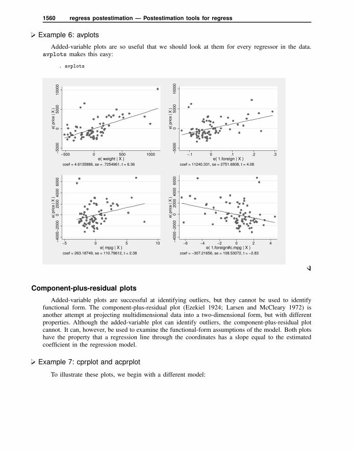
Example 6: avplots
Added-variable plots are so useful that we should look at them for every regressor in the data.avplots makes this easy:
. avplots
−5
00
00
50
00
10
00
0e
( p
rice
| X
)
−500 0 500 1000e( weight | X )
coef = 4.6135886, se = .7254961, t = 6.36
−5
00
00
50
00
10
00
0e
( p
rice
| X
)
−.1 0 .1 .2 .3e( 1.foreign | X )
coef = 11240.331, se = 2751.6808, t = 4.08
−4
00
0−
20
00
02
00
04
00
06
00
0e
( p
rice
| X
)
−5 0 5 10e( mpg | X )
coef = 263.18749, se = 110.79612, t = 2.38
−4
00
0−
20
00
02
00
04
00
06
00
0e
( p
rice
| X
)
−6 −4 −2 0 2 4e( 1.foreign#c.mpg | X )
coef = −307.21656, se = 108.53072, t = −2.83
Componentplusresidual plots
Added-variable plots are successful at identifying outliers, but they cannot be used to identifyfunctional form. The component-plus-residual plot (Ezekiel 1924; Larsen and McCleary 1972) isanother attempt at projecting multidimensional data into a two-dimensional form, but with differentproperties. Although the added-variable plot can identify outliers, the component-plus-residual plotcannot. It can, however, be used to examine the functional-form assumptions of the model. Both plotshave the property that a regression line through the coordinates has a slope equal to the estimatedcoefficient in the regression model.
Example 7: cprplot and acprplot
To illustrate these plots, we begin with a different model:
regress postestimation — Postestimation tools for regress 1561
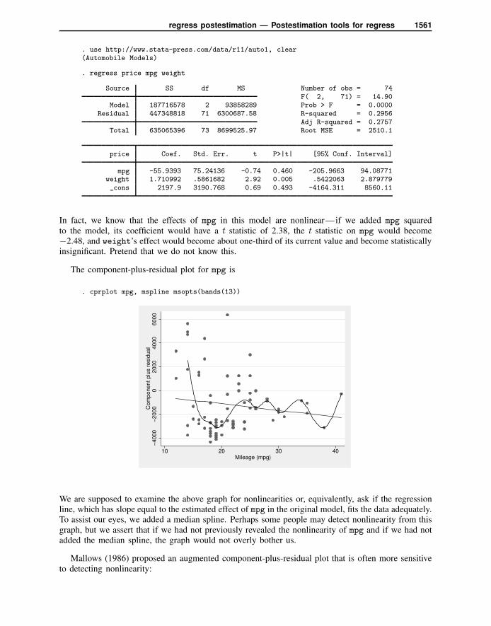
. use http://www.stata-press.com/data/r11/auto1, clear(Automobile Models)
. regress price mpg weight
Source SS df MS Number of obs = 74F( 2, 71) = 14.90
Model 187716578 2 93858289 Prob > F = 0.0000Residual 447348818 71 6300687.58 R-squared = 0.2956
Adj R-squared = 0.2757Total 635065396 73 8699525.97 Root MSE = 2510.1
price Coef. Std. Err. t P>|t| [95% Conf. Interval]
mpg -55.9393 75.24136 -0.74 0.460 -205.9663 94.08771weight 1.710992 .5861682 2.92 0.005 .5422063 2.879779_cons 2197.9 3190.768 0.69 0.493 -4164.311 8560.11
In fact, we know that the effects of mpg in this model are nonlinear—if we added mpg squaredto the model, its coefficient would have a t statistic of 2.38, the t statistic on mpg would become−2.48, and weight’s effect would become about one-third of its current value and become statisticallyinsignificant. Pretend that we do not know this.
The component-plus-residual plot for mpg is
. cprplot mpg, mspline msopts(bands(13))
−4000
−2000
02000
4000
6000
Com
ponent plu
s r
esid
ual
10 20 30 40Mileage (mpg)
We are supposed to examine the above graph for nonlinearities or, equivalently, ask if the regressionline, which has slope equal to the estimated effect of mpg in the original model, fits the data adequately.To assist our eyes, we added a median spline. Perhaps some people may detect nonlinearity from thisgraph, but we assert that if we had not previously revealed the nonlinearity of mpg and if we had notadded the median spline, the graph would not overly bother us.
Mallows (1986) proposed an augmented component-plus-residual plot that is often more sensitiveto detecting nonlinearity:

1562 regress postestimation — Postestimation tools for regress
. acprplot mpg, mspline msopts(bands(13))
−15000
−10000
−5000
Augm
ente
d c
om
ponent plu
s r
esid
ual
10 20 30 40Mileage (mpg)
It does do somewhat better.
Residualversuspredictor plots
Example 8: rvpplot
The residual-versus-predictor plot is a simple way to look for violations of the regression assumptions.If the assumptions are correct, there should be no pattern in the graph. Using our price on mpg andweight model, we type
. rvpplot mpg, yline(0)
−5000
05000
10000
Resid
uals
10 20 30 40Mileage (mpg)
Remember, any pattern counts as a problem, and in this graph, we see that the variation in theresiduals decreases as mpg increases.

regress postestimation — Postestimation tools for regress 1563
Leverage statistics
In addition to providing fitted values and the associated standard errors, the predict command canalso be used to generate various statistics used to detect the influence of individual observations. Thissection provides a brief introduction to leverage (hat) statistics, and some of the following subsectionsdiscuss other influence statistics produced by predict.
Example 9: diagonal elements of projection matrix
The diagonal elements of the projection matrix, obtained by the hat option, are a measure ofdistance in explanatory variable space. leverage is a synonym for hat.
. use http://www.stata-press.com/data/r11/auto(1978 Automobile Data)
. regress mpg weight c.weight#c.weight foreign
(output omitted )
. predict xdist, hat
. summarize xdist, detail
Leverage
Percentiles Smallest1% .0251334 .02513345% .0255623 .0251334
10% .0259213 .0253883 Obs 7425% .0278442 .0255623 Sum of Wgt. 74
50% .04103 Mean .0540541Largest Std. Dev. .0459218
75% .0631279 .159360690% .0854584 .1593606 Variance .002108895% .1593606 .2326124 Skewness 3.44080999% .3075759 .3075759 Kurtosis 16.95135
Some 5% of our sample has an xdist measure in excess of 0.15. Let’s force them to reveal theiridentities:
. list foreign make mpg if xdist>.15, divider
foreign make mpg
24. Domestic Ford Fiesta 2826. Domestic Linc. Continental 1227. Domestic Linc. Mark V 1243. Domestic Plym. Champ 34
To understand why these cars are on this list, we must remember that the explanatory variables in ourmodel are weight and foreign and that xdist measures distance in this metric. The Ford Fiestaand the Plymouth Champ are the two lightest domestic cars in our data. The Lincolns are the twoheaviest domestic cars.

1564 regress postestimation — Postestimation tools for regress
LR plots
Example 10: lvr2plot
One of the most useful diagnostic graphs is provided by lvr2plot (leverage-versus-residual-squaredplot), a graph of leverage against the (normalized) residuals squared.
. use http://www.stata-press.com/data/r11/auto, clear(1978 Automobile Data)
. regress price weight foreign##c.mpg
(output omitted )
. lvr2plot0
.1.2
.3.4
Levera
ge
0 .05 .1 .15 .2Normalized residual squared
The lines on the chart show the average values of leverage and the (normalized) residuals squared.Points above the horizontal line have higher-than-average leverage; points to the right of the verticalline have larger-than-average residuals.
One point immediately catches our eye, and four more make us pause. The point at the top of thegraph has high leverage and a smaller-than-average residual. The other points that bother us all havehigher-than-average leverage, two with smaller-than-average residuals and two with larger-than-averageresiduals.
A less pretty but more useful version of the above graph specifies that make be used as the symbol(see [G] marker label options):

regress postestimation — Postestimation tools for regress 1565
. lvr2plot, mlabel(make) mlabp(0) m(none) mlabsize(small)
AMC ConcordAMC PacerAMC Spirit
Buick Century
Buick Electra
Buick LeSabre
Buick Opel
Buick RegalBuick Riviera
Buick Skylark
Cad. Deville Cad. Eldorado
Cad. Seville
Chev. Chevette
Chev. ImpalaChev. MalibuChev. Monte Carlo
Chev. MonzaChev. Nova
Dodge Colt
Dodge DiplomatDodge MagnumDodge St. Regis
Ford Fiesta
Ford Mustang
Linc. ContinentalLinc. Mark V
Linc. VersaillesMerc. BobcatMerc. CougarMerc. Marquis
Merc. Monarch
Merc. XR−7Merc. Zephyr
Olds 98
Olds Cutl SuprOlds CutlassOlds Delta 88Olds OmegaOlds StarfireOlds Toronado
Plym. ArrowPlym. Champ
Plym. HorizonPlym. Sapporo
Plym. VolarePont. CatalinaPont. FirebirdPont. Grand PrixPont. Le MansPont. PhoenixPont. Sunbird
Audi 5000
Audi FoxBMW 320iDatsun 200
Datsun 210
Datsun 510
Datsun 810Fiat Strada
Honda Accord
Honda CivicMazda GLC
Peugeot 604
Renault Le Car
Subaru
Toyota CelicaToyota CorollaToyota Corona
VW Dasher
VW Diesel
VW RabbitVW Scirocco
Volvo 2600
.1.2
.3.4
Levera
ge
0 .05 .1 .15 .2Normalized residual squared
The VW Diesel, Plymouth Champ, Plymouth Arrow, and Peugeot 604 are the points that cause us themost concern. When we further examine our data, we discover that the VW Diesel is the only dieselin our data and that the data for the Plymouth Arrow were entered incorrectly into the computer. Nosuch simple explanations were found for the Plymouth Champ and Peugeot 604.
Standardized and studentized residuals
The terms standardized and studentized residuals have meant different things to different authors.In Stata, predict defines the standardized residual as ei = ei/(s
√1 − hi) and the studentized
residual as ri = ei/(s(i)√
1 − hi), where s(i) is the root mean squared error of a regression with theith observation removed. Stata’s definition of the studentized residual is the same as the one givenin Bollen and Jackman (1990, 264) and is what Chatterjee and Hadi (1988, 74) call the “externallystudentized” residual. Stata’s “standardized” residual is the same as what Chatterjee and Hadi (1988,74) call the “internally studentized” residual.
Standardized and studentized residuals are attempts to adjust residuals for their standard errors.Although the ǫi theoretical residuals are homoskedastic by assumption (i.e., they all have the samevariance), the calculated ei are not. In fact,
Var(ei) = σ2(1 − hi)
where hi are the leverage measures obtained from the diagonal elements of hat matrix. Thusobservations with the greatest leverage have corresponding residuals with the smallest variance.
Standardized residuals use the root mean squared error of the regression for σ. Studentized residualsuse the root mean squared error of a regression omitting the observation in question for σ. In general,studentized residuals are preferable to standardized residuals for purposes of outlier identification.Studentized residuals can be interpreted as the t statistic for testing the significance of a dummyvariable equal to 1 in the observation in question and 0 elsewhere (Belsley, Kuh, and Welsch 1980).Such a dummy variable would effectively absorb the observation and so remove its influence indetermining the other coefficients in the model. Caution must be exercised here, however, becauseof the simultaneous testing problem. You cannot simply list the residuals that would be individuallysignificant at the 5% level—their joint significance would be far less (their joint significance levelwould be far greater).
1566 regress postestimation — Postestimation tools for regress
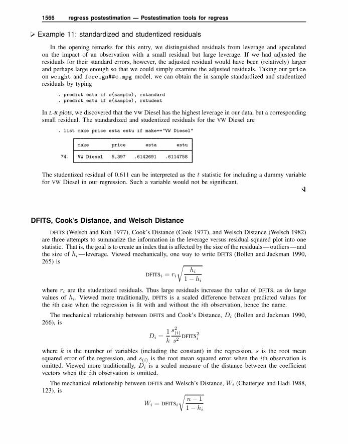
Example 11: standardized and studentized residuals
In the opening remarks for this entry, we distinguished residuals from leverage and speculatedon the impact of an observation with a small residual but large leverage. If we had adjusted theresiduals for their standard errors, however, the adjusted residual would have been (relatively) largerand perhaps large enough so that we could simply examine the adjusted residuals. Taking our priceon weight and foreign##c.mpg model, we can obtain the in-sample standardized and studentizedresiduals by typing
. predict esta if e(sample), rstandard
. predict estu if e(sample), rstudent
In L-R plots, we discovered that the VW Diesel has the highest leverage in our data, but a correspondingsmall residual. The standardized and studentized residuals for the VW Diesel are
. list make price esta estu if make=="VW Diesel"
make price esta estu
74. VW Diesel 5,397 .6142691 .6114758
The studentized residual of 0.611 can be interpreted as the t statistic for including a dummy variablefor VW Diesel in our regression. Such a variable would not be significant.
DFITS, Cook’s Distance, and Welsch Distance
DFITS (Welsch and Kuh 1977), Cook’s Distance (Cook 1977), and Welsch Distance (Welsch 1982)are three attempts to summarize the information in the leverage versus residual-squared plot into onestatistic. That is, the goal is to create an index that is affected by the size of the residuals—outliers—andthe size of hi—leverage. Viewed mechanically, one way to write DFITS (Bollen and Jackman 1990,265) is
DFITSi = ri
√hi
1 − hi
where ri are the studentized residuals. Thus large residuals increase the value of DFITS, as do largevalues of hi. Viewed more traditionally, DFITS is a scaled difference between predicted values forthe ith case when the regression is fit with and without the ith observation, hence the name.
The mechanical relationship between DFITS and Cook’s Distance, Di (Bollen and Jackman 1990,266), is
Di =1
k
s2(i)
s2DFITS
2i
where k is the number of variables (including the constant) in the regression, s is the root meansquared error of the regression, and s(i) is the root mean squared error when the ith observation isomitted. Viewed more traditionally, Di is a scaled measure of the distance between the coefficientvectors when the ith observation is omitted.
The mechanical relationship between DFITS and Welsch’s Distance, Wi (Chatterjee and Hadi 1988,123), is
Wi = DFITSi
√n− 1
1 − hi

regress postestimation — Postestimation tools for regress 1567
The interpretation of Wi is more difficult, as it is based on the empirical influence curve. AlthoughDFITS and Cook’s distance are similar, the Welsch distance measure includes another normalizationby leverage.
Belsley, Kuh, and Welsch (1980, 28) suggest that DFITS values greater than 2√k/n deserve more
investigation, and so values of Cook’s distance greater than 4/n should also be examined (Bollenand Jackman 1990, 265–266). Through similar logic, the cutoff for Welsch distance is approximately
3√k (Chatterjee and Hadi 1988, 124).
Example 12: DFITS influence measure
Using our model of price on weight and foreign##c.mpg, we can obtain the DFITS influencemeasure:
. use http://www.stata-press.com/data/r11/auto, clear(1978 Automobile Data)
. regress price weight foreign##c.mpg
(output omitted )
. predict e if e(sample), resid
. predict dfits, dfits
We did not specify if e(sample) in computing the DFITS statistic. DFITS is available only over theestimation sample, so specifying if e(sample) would have been redundant. It would have done noharm, but it would not have changed the results.
Our model has k = 5 independent variables (k includes the constant) and n = 74 observations;
following the 2√k/n cutoff advice, we type
. list make price e dfits if abs(dfits) > 2*sqrt(5/74), divider
make price e dfits
12. Cad. Eldorado 14,500 7271.96 .956445513. Cad. Seville 15,906 5036.348 1.35661924. Ford Fiesta 4,389 3164.872 .572417227. Linc. Mark V 13,594 3109.193 .520041328. Linc. Versailles 13,466 6560.912 .8760136
42. Plym. Arrow 4,647 -3312.968 -.9384231
We calculate Cook’s distance and list the observations greater than the suggested 4/n cutoff:
(Continued on next page)

1568 regress postestimation — Postestimation tools for regress
. predict cooksd if e(sample), cooksd
. list make price e cooksd if cooksd > 4/74, divider
make price e cooksd
12. Cad. Eldorado 14,500 7271.96 .149267613. Cad. Seville 15,906 5036.348 .332851524. Ford Fiesta 4,389 3164.872 .063881528. Linc. Versailles 13,466 6560.912 .130800442. Plym. Arrow 4,647 -3312.968 .1700736
Here we used if e(sample) because Cook’s distance is not restricted to the estimation sample bydefault. It is worth comparing this list with the preceding one.
Finally, we use Welsch distance and the suggested 3√k cutoff:
. predict wd, welsch
. list make price e wd if abs(wd) > 3*sqrt(5), divider
make price e wd
12. Cad. Eldorado 14,500 7271.96 8.39437213. Cad. Seville 15,906 5036.348 12.8112528. Linc. Versailles 13,466 6560.912 7.70300542. Plym. Arrow 4,647 -3312.968 -8.981481
Here we did not need to specify if e(sample) because welsch automatically restricts the predictionto the estimation sample.
COVRATIO
COVRATIO (Belsley, Kuh, and Welsch 1980) measures the influence of the ith observation byconsidering the effect on the variance–covariance matrix of the estimates. The measure is the ratioof the determinants of the covariances matrix, with and without the ith observation. The resultingformula is
COVRATIOi =1
1 − hi
(n− k − e2in− k − 1
)k
where ei is the standardized residual.
For noninfluential observations, the value of COVRATIO is approximately 1. Large values of theresiduals or large values of leverage will cause deviations from 1, although if both are large, COVRATIOmay tend back toward 1 and therefore not identify such observations (Chatterjee and Hadi 1988, 139).
Belsley, Kuh, and Welsch (1980) suggest that observations for which
|COVRATIOi − 1| ≥ 3k
n
are worthy of further examination.

regress postestimation — Postestimation tools for regress 1569
Example 13: COVRATIO influence measure
Using our model of price on weight and foreign##c.mpg, we can obtain the COVRATIO
measure and list the observations outside the suggested cutoff by typing
. predict covr, covratio
. list make price e covr if abs(covr-1) >= 3*5/74, divider
make price e covr
12. Cad. Eldorado 14,500 7271.96 .381424213. Cad. Seville 15,906 5036.348 .738696928. Linc. Versailles 13,466 6560.912 .476169543. Plym. Champ 4,425 1621.747 1.2778253. Audi 5000 9,690 591.2883 1.206842
57. Datsun 210 4,589 19.81829 1.28480164. Peugeot 604 12,990 1037.184 1.34821966. Subaru 3,798 -909.5894 1.26467771. VW Diesel 5,397 999.7209 1.63065374. Volvo 260 11,995 1327.668 1.211888
The covratio option automatically restricts the prediction to the estimation sample.
DFBETAs
DFBETAs are perhaps the most direct influence measure of interest to model builders. DFBETAsfocus on one coefficient and measure the difference between the regression coefficient when the ithobservation is included and excluded, the difference being scaled by the estimated standard error ofthe coefficient. Belsley, Kuh, and Welsch (1980, 28) suggest observations with |DFBETAi| > 2/
√n
as deserving special attention, but it is also common practice to use 1 (Bollen and Jackman 1990,267), meaning that the observation shifted the estimate at least one standard error.
Example 14: DFBETAs influence measure; the dfbeta() option
Using our model of price on weight and foreign##c.mpg, let’s first ask which observationshave the greatest impact on the determination of the coefficient on 1.foreign. We will use thesuggested 2/
√n cutoff:
. sort foreign make
. predict dfor, dfbeta(1.foreign)
. list make price foreign dfor if abs(dfor) > 2/sqrt(74), divider
make price foreign dfor
12. Cad. Eldorado 14,500 Domestic -.529051913. Cad. Seville 15,906 Domestic .824341928. Linc. Versailles 13,466 Domestic -.528372942. Plym. Arrow 4,647 Domestic -.662242443. Plym. Champ 4,425 Domestic .2371104
64. Peugeot 604 12,990 Foreign .255203269. Toyota Corona 5,719 Foreign -.256431
The Cadillac Seville shifted the coefficient on 1.foreign 0.82 standard deviations!

1570 regress postestimation — Postestimation tools for regress
Now let us ask which observations have the greatest effect on the mpg coefficient:
. predict dmpg, dfbeta(mpg)
. list make price mpg dmpg if abs(dmpg) > 2/sqrt(74), divider
make price mpg dmpg
12. Cad. Eldorado 14,500 14 -.597035113. Cad. Seville 15,906 21 1.13426928. Linc. Versailles 13,466 14 -.606928742. Plym. Arrow 4,647 28 -.892585943. Plym. Champ 4,425 34 .3186909
Once again we see the Cadillac Seville heading the list, indicating that our regression results may bedominated by this one car.
Example 15: DFBETAs influence measure; the dfbeta command
We can use predict, dfbeta() or the dfbeta command to generate the DFBETAs. dfbetamakes up names for the new variables automatically and, without arguments, generates the DFBETAsfor all the variables in the regression:
. dfbeta_dfbeta_1: dfbeta(weight)_dfbeta_2: dfbeta(1.foreign)_dfbeta_3: dfbeta(mpg)_dfbeta_4: dfbeta(1.foreign#c.mpg)
dfbeta created four new variables in our dataset: dfbeta 1, containing the DFBETAs for weight;dfbeta 2, containing the DFBETAs for mpg; and so on. Had we wanted only the DFBETAs for mpg
and weight, we might have typed
. dfbeta mpg weight_dfbeta_5: dfbeta(weight)_dfbeta_6: dfbeta(mpg)
In the example above, we typed dfbeta mpg weight instead of dfbeta; if we had typed dfbetafollowed by dfbeta mpg weight, here is what would have happened:
. dfbeta_dfbeta_7: dfbeta(weight)_dfbeta_8: dfbeta(1.foreign)_dfbeta_9: dfbeta(mpg)_dfbeta_10: dfbeta(1.foreign#c.mpg)
. dfbeta mpg weight_dfbeta_11: dfbeta(weight)_dfbeta_12: dfbeta(mpg)
dfbeta would have made up different names for the new variables. dfbeta never replaces existingvariables—it instead makes up a different name, so we need to pay attention to dfbeta’s output.

regress postestimation — Postestimation tools for regress 1571
Formal tests for violations of assumptions
This section introduces some regression diagnostic commands that are designed to test for certain vio-lations that rvfplot less formally attempts to detect. estat ovtest provides Ramsey’s test for omittedvariables—a pattern in the residuals. estat hettest provides a test for heteroskedasticity—theincreasing or decreasing variation in the residuals with fitted values, with respect to the explanatoryvariables, or with respect to yet other variables. The score test implemented in estat hettest(Breusch and Pagan 1979; Cook and Weisberg 1983) performs a score test of the null hypothesisthat b = 0 against the alternative hypothesis of multiplicative heteroskedasticity. estat szroeterprovides a rank test for heteroskedasticity, which is an alternative to the score test computed by estathettest. Finally, estat imtest computes an information matrix test, including an orthogonal de-composition into tests for heteroskedasticity, skewness, and kurtosis (Cameron and Trivedi 1990). Theheteroskedasticity test computed by estat imtest is similar to the general test for heteroskedasticitythat was proposed by White (1980). Cameron and Trivedi (2009, chap. 3) discuss most of these testsand provides more examples.
Example 16: estat ovtest, estat hettest, estat szroeter, and estat imtest
We run these commands just mentioned on our model:
. estat ovtest
Ramsey RESET test using powers of the fitted values of priceHo: model has no omitted variables
F(3, 66) = 7.77Prob > F = 0.0002
. estat hettest
Breusch-Pagan / Cook-Weisberg tests for heteroskedasticityHo: Constant variancevariables: fitted values of price
chi2(1) = 6.50Prob > chi2 = 0.0108
Testing for heteroskedasticity in the right-hand-side variables is requested by specifying the rhsoption. By specifying the mtest(bonferroni) option, we request that tests be conducted for eachof the variables, with a Bonferroni adjustment for the p-values to accommodate our testing multiplehypotheses.
. estat hettest, rhs mtest(bonf)
Breusch-Pagan / Cook-Weisberg test for heteroskedasticityHo: Constant variance
Variable chi2 df p
weight 15.24 1 0.0004 #1.foreign 6.15 1 0.0525 #
mpg 9.04 1 0.0106 #foreign#c.mpg
1 6.02 1 0.0566 #
simultaneous 15.60 4 0.0036
# Bonferroni adjusted p-values

1572 regress postestimation — Postestimation tools for regress
. estat szroeter, rhs mtest(holm)
Szroeter’s test for homoskedasticity
Ho: variance constantHa: variance monotonic in variable
Variable chi2 df p
weight 17.07 1 0.0001 #1.foreign 6.15 1 0.0131 #
mpg 11.45 1 0.0021 #foreign#c.mpg
1 6.17 1 0.0260 #
# Holm adjusted p-values
Finally, we request the information matrix test, which is a conditional moments test with second-,third-, and fourth-order moment conditions.
. estat imtest
Cameron & Trivedi’s decomposition of IM-test
Source chi2 df p
Heteroskedasticity 18.86 10 0.0420Skewness 11.69 4 0.0198Kurtosis 2.33 1 0.1273
Total 32.87 15 0.0049
We find evidence for omitted variables, heteroskedasticity, and nonnormal skewness.
So, why bother with the various graphical commands when the tests seem so much easier tointerpret? In part, it is a matter of taste: both are designed to uncover the same problem, and bothare, in fact, going about it in similar ways. One is based on a formal calculation, whereas the other isbased on personal judgment in evaluating a graph. On the other hand, the tests are seeking evidenceof specific problems, whereas judgment is more general. The careful analyst will use both.
We performed the omitted-variable test first. Omitted variables are a more serious problem thanheteroskedasticity or the violations of higher moment conditions tested by estat imtest. If thiswere not a manual, having found evidence of omitted variables, we would never have run theestat hettest, estat szroeter, and estat imtest commands, at least not until we solved theomitted-variable problem.
Technical note
estat ovtest and estat hettest both perform two flavors of their respective tests. By default,estat ovtest looks for evidence of omitted variables by fitting the original model augmented byy2, y3, and y4, which are the fitted values from the original model. Under the assumption of nomisspecification, the coefficients on the powers of the fitted values will be zero. With the rhs option,estat ovtest instead augments the original model with powers (second through fourth) of theexplanatory variables (except for dummy variables).

regress postestimation — Postestimation tools for regress 1573
estat hettest, by default, looks for heteroskedasticity by modeling the variance as a functionof the fitted values. If, however, we specify a variable or variables, the variance will be modeled asa function of the specified variables. In our example, if we had, a priori, some reason to suspectheteroskedasticity and that the heteroskedasticity is a function of a car’s weight, then using a test thatfocuses on weight would be more powerful than the more general tests such as White’s test or thefirst term in the Cameron–Trivedi decomposition test.
estat hettest, by default, computes the original Breusch–Pagan/Cook–Weisberg test, whichincludes the assumption of normally distributed errors. Koenker (1981) derived an N ∗ R2 versionof this test that drops the normality assumption. Wooldridge (2009) gives an F statistic version thatdoes not require the normality assumption.
Variance inflation factors
Problems arise in regression when the predictors are highly correlated. In this situation, there maybe a significant change in the regression coefficients if you add or delete an independent variable.The estimated standard errors of the fitted coefficients are inflated, or the estimated coefficients maynot be statistically significant even though a statistical relation exists between the dependent andindependent variables.
Data analysts rely on these facts to check informally for the presence of multicollinearity. estatvif, another command for use after regress, calculates the variance inflation factors and tolerancesfor each of the independent variables.
The output shows the variance inflation factors together with their reciprocals. Some analystscompare the reciprocals with a predetermined tolerance. In the comparison, if the reciprocal of theVIF is smaller than the tolerance, the associated predictor variable is removed from the regressionmodel. However, most analysts rely on informal rules of thumb applied to the VIF; see Chatterjeeand Hadi (2006). According to these rules, there is evidence of multicollinearity if
1. The largest VIF is greater than 10 (some choose a more conservative threshold value of 30).
2. The mean of all the VIFs is considerably larger than 1.
Example 17: estat vif
We examine a regression model fit using the ubiquitous automobile dataset:
. regress price mpg rep78 trunk headroom length turn displ gear_ratio
Source SS df MS Number of obs = 69F( 8, 60) = 6.33
Model 264102049 8 33012756.2 Prob > F = 0.0000Residual 312694909 60 5211581.82 R-squared = 0.4579
Adj R-squared = 0.3856Total 576796959 68 8482308.22 Root MSE = 2282.9
price Coef. Std. Err. t P>|t| [95% Conf. Interval]
mpg -144.84 82.12751 -1.76 0.083 -309.1195 19.43948rep78 727.5783 337.6107 2.16 0.035 52.25638 1402.9trunk 44.02061 108.141 0.41 0.685 -172.2935 260.3347
headroom -807.0996 435.5802 -1.85 0.069 -1678.39 64.19061length -8.688914 34.89848 -0.25 0.804 -78.49626 61.11843
turn -177.9064 137.3455 -1.30 0.200 -452.6383 96.82551displacement 30.73146 7.576952 4.06 0.000 15.5753 45.88762
gear_ratio 1500.119 1110.959 1.35 0.182 -722.1303 3722.368_cons 6691.976 7457.906 0.90 0.373 -8226.057 21610.01

1574 regress postestimation — Postestimation tools for regress
. estat vif
Variable VIF 1/VIF
length 8.22 0.121614displacement 6.50 0.153860
turn 4.85 0.205997gear_ratio 3.45 0.290068
mpg 3.03 0.330171trunk 2.88 0.347444
headroom 1.80 0.554917rep78 1.46 0.686147
Mean VIF 4.02
The results are mixed. Although we have no VIFs greater than 10, the mean VIF is greater than 1,though not considerably so. We could continue the investigation of collinearity, but given that otherauthors advise that collinearity is a problem only when VIFs exist that are greater than 30 (contradictingour rule above), we will not do so here.
Example 18: estat vif, with strong evidence of multicollinearity
This example comes from a dataset described in Kutner, Nachtsheim, and Neter (2004, 257) thatexamines body fat as modeled by caliper measurements on the triceps, midarm, and thigh.
. use http://www.stata-press.com/data/r11/bodyfat, clear(Body Fat)
. regress bodyfat tricep thigh midarm
Source SS df MS Number of obs = 20F( 3, 16) = 21.52
Model 396.984607 3 132.328202 Prob > F = 0.0000Residual 98.4049068 16 6.15030667 R-squared = 0.8014
Adj R-squared = 0.7641Total 495.389513 19 26.0731323 Root MSE = 2.48
bodyfat Coef. Std. Err. t P>|t| [95% Conf. Interval]
triceps 4.334085 3.015511 1.44 0.170 -2.058512 10.72668thigh -2.856842 2.582015 -1.11 0.285 -8.330468 2.616785midarm -2.186056 1.595499 -1.37 0.190 -5.568362 1.19625_cons 117.0844 99.78238 1.17 0.258 -94.44474 328.6136
. estat vif
Variable VIF 1/VIF
triceps 708.84 0.001411thigh 564.34 0.001772midarm 104.61 0.009560
Mean VIF 459.26
Here we see strong evidence of multicollinearity in our model. More investigation reveals that themeasurements on the thigh and the triceps are highly correlated:
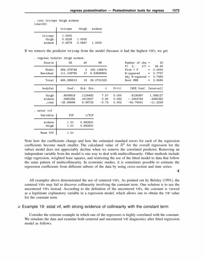
regress postestimation — Postestimation tools for regress 1575
. corr triceps thigh midarm(obs=20)
triceps thigh midarm
triceps 1.0000thigh 0.9238 1.0000midarm 0.4578 0.0847 1.0000
If we remove the predictor tricep from the model (because it had the highest VIF), we get
. regress bodyfat thigh midarm
Source SS df MS Number of obs = 20F( 2, 17) = 29.40
Model 384.279748 2 192.139874 Prob > F = 0.0000Residual 111.109765 17 6.53586854 R-squared = 0.7757
Adj R-squared = 0.7493Total 495.389513 19 26.0731323 Root MSE = 2.5565
bodyfat Coef. Std. Err. t P>|t| [95% Conf. Interval]
thigh .8508818 .1124482 7.57 0.000 .6136367 1.088127midarm .0960295 .1613927 0.60 0.560 -.2444792 .4365383_cons -25.99696 6.99732 -3.72 0.002 -40.76001 -11.2339
. estat vif
Variable VIF 1/VIF
midarm 1.01 0.992831thigh 1.01 0.992831
Mean VIF 1.01
Note how the coefficients change and how the estimated standard errors for each of the regressioncoefficients become much smaller. The calculated value of R2 for the overall regression for thesubset model does not appreciably decline when we remove the correlated predictor. Removing anindependent variable from the model is one way to deal with multicollinearity. Other methods includeridge regression, weighted least squares, and restricting the use of the fitted model to data that followthe same pattern of multicollinearity. In economic studies, it is sometimes possible to estimate theregression coefficients from different subsets of the data by using cross-section and time series.
All examples above demonstrated the use of centered VIFs. As pointed out by Belsley (1991), thecentered VIFs may fail to discover collinearity involving the constant term. One solution is to use theuncentered VIFs instead. According to the definition of the uncentered VIFs, the constant is viewedas a legitimate explanatory variable in a regression model, which allows one to obtain the VIF valuefor the constant term.
Example 19: estat vif, with strong evidence of collinearity with the constant term
Consider the extreme example in which one of the regressors is highly correlated with the constant.We simulate the data and examine both centered and uncentered VIF diagnostics after fitted regressionmodel as follows.
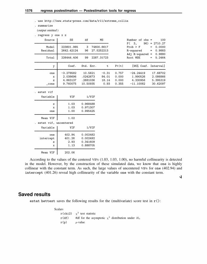
1576 regress postestimation — Postestimation tools for regress
. use http://www.stata-press.com/data/r11/extreme_collin
. summarize
(output omitted )
. regress y one x z
Source SS df MS Number of obs = 100F( 3, 96) = 2710.27
Model 223801.985 3 74600.6617 Prob > F = 0.0000Residual 2642.42124 96 27.5252213 R-squared = 0.9883
Adj R-squared = 0.9880Total 226444.406 99 2287.31723 Root MSE = 5.2464
y Coef. Std. Err. t P>|t| [95% Conf. Interval]
one -3.278582 10.5621 -0.31 0.757 -24.24419 17.68702x 2.038696 .0242673 84.01 0.000 1.990526 2.086866z 4.863137 .2681036 18.14 0.000 4.330956 5.395319
_cons 9.760075 10.50935 0.93 0.355 -11.10082 30.62097
. estat vif
Variable VIF 1/VIF
z 1.03 0.968488x 1.03 0.971307
one 1.00 0.995425
Mean VIF 1.02
. estat vif, uncentered
Variable VIF 1/VIF
one 402.94 0.002482intercept 401.26 0.002492
z 2.93 0.341609x 1.13 0.888705
Mean VIF 202.06
According to the values of the centered VIFs (1.03, 1.03, 1.00), no harmful collinearity is detectedin the model. However, by the construction of these simulated data, we know that one is highlycollinear with the constant term. As such, the large values of uncentered VIFs for one (402.94) andintercept (401.26) reveal high collinearity of the variable one with the constant term.
Saved results
estat hettest saves the following results for the (multivariate) score test in r():
Scalars
r(chi2) χ2 test statistic
r(df) #df for the asymptotic χ2 distribution under H0
r(p) p-value

regress postestimation — Postestimation tools for regress 1577
estat hettest, fstat saves results for the (multivariate) score test in r():
Scalars
r(F) test statistic
r(df m) #df of the test for the F distribution under H0
r(df r) #df of the residuals for the F distribution under H0
r(p) p-value
estat hettest (if mtest is specified) and estat szroeter save the following in r():
Matrices
r(mtest) a matrix of test results, with rows corresponding to the univariate tests
mtest[.,1] χ2 test statistic
mtest[.,2] #df
mtest[.,3] unadjusted p-value
mtest[.,4] adjusted p-value (if an mtest() adjustment method is specified)
Macros
r(mtmethod) adjustment method for p-values
estat imtest saves the following in r():
Scalars
r(chi2 t) IM-test statistic (= r(chi2 h) + r(chi2 s) + r(chi2 k))r(df t) df for limiting χ2 distribution under H0 (= r(df h) + r(df s) + r(df k))r(chi2 h) heteroskedasticity test statistic
r(df h) df for limiting χ2 distribution under H0
r(chi2 s) skewness test statistic
r(df s) df for limiting χ2 distribution under H0
r(chi2 k) kurtosis test statistic
r(df k) df for limiting χ2 distribution under H0
r(chi2 w) White’s heteroskedasticity test (if white specified)
r(df w) df for limiting χ2 distribution under H0
estat ovtest saves the following in r():
Scalars
r(p) two-sided p-value r(df) degrees of freedom
r(F) F statistic r(df r) residual degrees of freedom
Methods and formulas
All regression fit and diagnostic commands are implemented as ado-files.
See Hamilton (2009, chap. 7), Kohler and Kreuter (2009, sec. 8.3), or Baum (2006, chap. 5) foran overview of using Stata to perform regression diagnostics. See Peracchi (2001, chap. 8) for amathematically rigorous discussion of diagnostics.

1578 regress postestimation — Postestimation tools for regress
Methods and formulas for predict
Assume that you have already fit the regression model
y = Xb + e
where X is n× k.
Denote the previously estimated coefficient vector by b and its estimated variance matrix by V.predict works by recalling various aspects of the model, such as b, and combining that informationwith the data currently in memory. Let xj be the jth observation currently in memory, and let s2 bethe mean squared error of the regression.
Let V = s2(X′X)−1. Let k be the number of independent variables including the intercept, ifany, and let yj be the observed value of the dependent variable.
The predicted value (xb option) is defined as yj = xjb.
Let ℓj represent a lower bound for an observation j and uj represent an upper bound. Theprobability that yj |xj would be observed in the interval (ℓj , uj)—the pr(ℓ, u) option—is
P (ℓj , uj) = Pr(ℓj < xjb + ej < uj) = Φ
(uj − yj
s
)− Φ
(ℓj − yj
s
)
where for the pr(ℓ, u), e(ℓ, u), and ystar(ℓ, u) options, ℓj and uj can be anywhere in therange (−∞,+∞).
The option e(ℓ, u) computes the expected value of yj |xj conditional on yj|xj being in theinterval (ℓj, uj), that is, when yj|xj is censored. It can be expressed as
E(ℓj , uj) = E(xjb + ej | ℓj < xjb + ej < uj) = yj − sφ(
uj−yj
s
)− φ
(ℓj−yj
s
)
Φ(
uj−yj
s
)− Φ
(ℓj−yj
s
)
where φ is the normal density and Φ is the cumulative normal.
You can also compute ystar(ℓ, u)—the expected value of yj |xj , where yj is assumed truncatedat ℓj and uj :
y∗j =
ℓj if xjb + ej ≤ ℓjxjb + u if ℓj < xjb + ej < uj
uj if xjb + ej ≥ uj
This computation can be expressed in several ways, but the most intuitive formulation involves acombination of the two statistics just defined:
y∗j = P (−∞, ℓj)ℓj + P (ℓj , uj)E(ℓj , uj) + P (uj,+∞)uj
A diagonal element of the projection matrix (hat) or (leverage) is given by
hj = xj(X′X)−1x′
j
The standard error of the prediction (the stdp option) is defined as spj=√
xjVx′j
and can also be written as spj= s√hj .

regress postestimation — Postestimation tools for regress 1579
The standard error of the forecast (stdf) is defined as sfj= s√
1 + hj .
The standard error of the residual (stdr) is defined as srj= s√
1− hj .
The residuals (residuals) are defined as ej = yj − yj .
The standardized residuals (rstandard) are defined as esj= ej/srj
.
The studentized residuals (rstudent) are defined as
rj =ej
s(j)√
1 − hj
where s(j) represents the root mean squared error with the jth observation removed, which is givenby
s2(j) =s2(T − k)
T − k − 1−
e 2j
(T − k − 1)(1 − hj)
Cook’s D (cooksd) is given by
Dj =e 2
sj(spj
/srj)2
k=
hj e2j
ks2(1 − hj)2
DFITS (dfits) is given by
DFITSj = rj
√hj
1 − hj
Welsch distance (welsch) is given by
Wj =rj√hj(n− 1)
1 − hj
COVRATIO (covratio) is given by
COVRATIOj =1
1 − hj
(n− k − e2jn− k − 1
)k
The DFBETAs (dfbeta) for a particular regressor xi are given by
DFBETAj =rjuj√
U2(1 − hj)
where uj are the residuals obtained from a regression of xj on the remaining x’s and U2 =∑j
u2j .
The omitted-variable test (Ramsey 1969) reported by ovtest fits the regression yi = xib+zit+ui
and then performs a standard F test of t = 0. The default test uses zi = (y2i , y
3i , y
4i ). If rhs is
specified, zi = (x21i, x
31i, x
41i, x
22i, . . . , x
4mi). In either case, the variables are normalized to have
minimum 0 and maximum 1 before powers are calculated.

1580 regress postestimation — Postestimation tools for regress
The test for heteroskedasticity (Breusch and Pagan 1979; Cook and Weisberg 1983) modelsVar(ei) = σ2 exp(zt), where z is a variable list specified by the user, the list of right-hand-side
variables, or the fitted values xβ. The test is of t = 0. Mechanically, estat hettest fits theaugmented regression e2i /σ
2 = a+ zit + vi.
The original Breusch–Pagan/Cook–Weisberg version of the test assumes that the ei are normallydistributed under the null hypothesis which implies that the score test statistic S is equal to the modelsum of squares from the augmented regression divided by 2. Under the null hypothesis, S has theχ2 distribution with m degrees of freedom, where m is the number of columns of z.
Koenker (1981) derived a score test of the null hypothesis that t = 0 under the assumption thatthe ei are independent and identically distributed (i.i.d.). Koenker showed that S = N ∗ R2 has alarge-sample χ2 distribution with m degrees of freedom, where N is the number of observationsand R2 is the R-squared in the augmented regression and m is the number of columns of z. estathettest, iid produces this version of the test.
Wooldridge (2009) showed that an F test of t = 0 in the augmented regression can also be usedunder the assumption that the ei are i.i.d. estat hettest, fstat produces this version of the test.
Szroeter’s class of tests for homoskedasticity against the alternative that the residual varianceincreases in some variable x is defined in terms of
H =
∑ni=1 h(xi)e
2i∑n
i=1 e2i
where h(x) is some weight function that increases in x (Szroeter 1978). H is a weighted averageof the h(x), with the squared residuals serving as weights. Under homoskedasticity, H should beapproximately equal to the unweighted average of h(x). Large values of H suggest that e2i tends to belarge where h(x) is large; i.e., the variance indeed increases in x, whereas small values of H suggestthat the variance actually decreases in x. estat szroeter uses h(xi) = rank(xi in x1 . . . xn); seeJudge et al. [1985, 452] for details. estat szroeter displays a normalized version of H ,
Q =
√6n
n2 − 1H
which is approximately N(0, 1) distributed under the null (homoskedasticity).
estat hettest and estat szroeter provide adjustments of p-values for multiple testing. Thesupported methods are described in [R] test.
estat imtest performs the information matrix test for the regression model, as well as anorthogonal decomposition into tests for heteroskedasticity δ1, nonnormal skewness δ2, and nonnormalkurtosis δ3 (Cameron and Trivedi 1990; Long and Trivedi 1992). The decomposition is obtained viathree auxiliary regressions. Let e be the regression residuals, σ2 be the maximum likelihood estimateof σ2 in the regression, n be the number of observations, X be the set of k variables specified withestat imtest, and R2
un be the uncentered R2 from a regression. δ1 is obtained as nR2un from a
regression of e2 − σ2 on the cross-products of the variables in X . δ2 is computed as nR2un from a
regression of e3−3σ2e on X . Finally, δ3 is obtained as nR2un from a regression of e4−6σ2e2−3σ4
on X . δ1, δ2, and δ3 are asymptotically χ2 distributed with 1/2k(k+1),K , and 1 degree of freedom.The information test statistic δ = δ1 + δ2 + δ3 is asymptotically χ2 distributed with 1/2k(k + 3)degrees of freedom. White’s test for heteroskedasticity is computed as nR2 from a regression of u2
on X and the cross-products of the variables in X . This test statistic is usually close to δ1.
estat vif calculates the centered variance inflation factor (VIFc) (Chatterjee and Hadi 2006,235–239) for xj , given by
regress postestimation — Postestimation tools for regress 1581
VIFc(xj) =1
1 − R2j
where R2j is the square of the centered multiple correlation coefficient that results when xj is regressed
with intercept against all the other explanatory variables.
The uncentered variance inflation factor (VIFuc) (Belsley 1991, 28–29) for xj is given by
VIFuc(xj) =1
1 − R2j
where R2j is the square of the uncentered multiple correlation coefficient that results when xj is
regressed without intercept against all the other explanatory variables including the constant term.
Acknowledgments
estat ovtest and estat hettest are based on programs originally written by Richard Goldstein(1991, 1992). estat imtest, estat szroeter, and the current version of estat hettest werewritten by Jeroen Weesie, Department of Sociology, Utrecht University, The Netherlands; estat
imtest is based in part on code written by J. Scott Long, Department of Sociology, IndianaUniversity.
ReferencesAdkins, L. C., and R. C. Hill. 2008. Using Stata for Principles of Econometrics. 3rd ed. Hoboken, NJ: Wiley.
Baum, C. F. 2006. An Introduction to Modern Econometrics Using Stata. College Station, TX: Stata Press.
Baum, C. F., N. J. Cox, and V. L. Wiggins. 2000. sg137: Tests for heteroskedasticity in regression error distribution.Stata Technical Bulletin 55: 15–17. Reprinted in Stata Technical Bulletin Reprints, vol. 10, pp. 147–149. CollegeStation, TX: Stata Press.
Baum, C. F., and V. L. Wiggins. 2000a. sg135: Test for autoregressive conditional heteroskedasticity in regressionerror distribution. Stata Technical Bulletin 55: 13–14. Reprinted in Stata Technical Bulletin Reprints, vol. 10, pp.143–144. College Station, TX: Stata Press.
. 2000b. sg136: Tests for serial correlation in regression error distribution. Stata Technical Bulletin 55: 14–15.Reprinted in Stata Technical Bulletin Reprints, vol. 10, pp. 145–147. College Station, TX: Stata Press.
Belsley, D. A. 1991. Conditional Diagnostics: Collinearity and Weak Data in Regression. New York: Wiley.
Belsley, D. A., E. Kuh, and R. E. Welsch. 1980. Regression Diagnostics: Identifying Influential Data and Sources ofCollinearity. New York: Wiley.
Bollen, K. A., and R. W. Jackman. 1990. Regression diagnostics: An expository treatment of outliers and influentialcases. In Modern Methods of Data Analysis, ed. J. Fox and J. S. Long, 257–291. Newbury Park, CA: Sage.
Breusch, T. S., and A. R. Pagan. 1979. A simple test for heteroscedasticity and random coefficient variation. Econometrica47: 1287–1294.
Cameron, A. C., and P. K. Trivedi. 1990. The information matrix test and its applied alternative hypotheses. Workingpaper 372, University of California–Davis, Institute of Governmental Affairs.
. 2009. Microeconometrics Using Stata. College Station, TX: Stata Press.
Chatterjee, S., and A. S. Hadi. 1986. Influential observations, high leverage points, and outliers in linear regression.Statistical Science 1: 379–393.
. 1988. Sensitivity Analysis in Linear Regression. New York: Wiley.
. 2006. Regression Analysis by Example. 4th ed. New York: Wiley.
Cook, R. D. 1977. Detection of influential observation in linear regression. Technometrics 19: 15–18.

1582 regress postestimation — Postestimation tools for regress
Cook, R. D., and S. Weisberg. 1982. Residuals and Influence in Regression. New York: Chapman & Hall/CRC.
. 1983. Diagnostics for heteroscedasticity in regression. Biometrika 70: 1–10.
Cox, N. J. 2004. Speaking Stata: Graphing model diagnostics. Stata Journal 4: 449–475.
DeMaris, A. 2004. Regression with Social Data: Modeling Continuous and Limited Response Variables. Hoboken, NJ:Wiley.
Ezekiel, M. 1924. A method of handling curvilinear correlation for any number of variables. Journal of the AmericanStatistical Association 19: 431–453.
Garrett, J. M. 2000. sg157: Predicted values calculated from linear or logistic regression models. Stata TechnicalBulletin 58: 27–30. Reprinted in Stata Technical Bulletin Reprints, vol. 10, pp. 258–261. College Station, TX:Stata Press.
Goldstein, R. 1991. srd5: Ramsey test for heteroscedasticity and omitted variables. Stata Technical Bulletin 2: 27.Reprinted in Stata Technical Bulletin Reprints, vol. 1, p. 177. College Station, TX: Stata Press.
. 1992. srd14: Cook–Weisberg test of heteroscedasticity. Stata Technical Bulletin 10: 27–28. Reprinted in StataTechnical Bulletin Reprints, vol. 2, pp. 183–184. College Station, TX: Stata Press.
Hamilton, L. C. 1992. Regression with Graphics: A Second Course in Applied Statistics. Belmont, CA: Duxbury.
. 2009. Statistics with Stata (Updated for Version 10). Belmont, CA: Brooks/Cole.
Hardin, J. W. 1995. sg32: Variance inflation factors and variance-decomposition proportions. Stata Technical Bulletin24: 17–22. Reprinted in Stata Technical Bulletin Reprints, vol. 4, pp. 154–160. College Station, TX: Stata Press.
Hill, R. C., W. E. Griffiths, and G. C. Lim. 2008. Principles of Econometrics. 3rd ed. Hoboken, NJ: Wiley.
Hoaglin, D. C., and P. J. Kempthorne. 1986. Comment [on Chatterjee and Hadi 1986]. Statistical Science 1: 408–412.
Hoaglin, D. C., and R. E. Welsch. 1978. The hat matrix in regression and ANOVA. American Statistician 32: 17–22.
Judge, G. G., W. E. Griffiths, R. C. Hill, H. Lutkepohl, and T.-C. Lee. 1985. The Theory and Practice of Econometrics.2nd ed. New York: Wiley.
Koenker, R. 1981. A note on studentizing a test for heteroskedasticity. Journal of Econometrics 17: 107–112.
Kohler, U., and F. Kreuter. 2009. Data Analysis Using Stata. 2nd ed. College Station, TX: Stata Press.
Kutner, M. H., C. J. Nachtsheim, and J. Neter. 2004. Applied Linear Regression Models. 4th ed. New York:McGraw–Hill/Irwin.
Larsen, W. A., and S. J. McCleary. 1972. The use of partial residual plots in regression analysis. Technometrics 14:781–790.
Long, J. S., and J. Freese. 2000. sg145: Scalar measures of fit for regression models. Stata Technical Bulletin 56:34–40. Reprinted in Stata Technical Bulletin Reprints, vol. 10, pp. 197–205. College Station, TX: Stata Press.
Long, J. S., and P. K. Trivedi. 1992. Some specification tests for the linear regression model. Sociological Methodsand Research 21: 161–204. Reprinted in Testing Structural Equation Models, ed. K. A. Bollen and J. S. Long, pp.66–110. Newbury Park, CA: Sage.
Mallows, C. L. 1986. Augmented partial residuals. Technometrics 28: 313–319.
Mosteller, F., and J. W. Tukey. 1977. Data Analysis and Regression: A Second Course in Statistics. Reading, MA:Addison–Wesley.
Peracchi, F. 2001. Econometrics. Chichester, UK: Wiley.
Ramsey, J. B. 1969. Tests for specification errors in classical linear least-squares regression analysis. Journal of theRoyal Statistical Society, Series B 31: 350–371.
Ramsey, J. B., and P. Schmidt. 1976. Some further results on the use of OLS and BLUS residuals in specificationerror tests. Journal of the American Statistical Association 71: 389–390.
Rousseeuw, P. J., and A. M. Leroy. 1987. Robust Regression and Outlier Detection. New York: Wiley.
Szroeter, J. 1978. A class of parametric tests for heteroscedasticity in linear econometric models. Econometrica 46:1311–1327.
Velleman, P. F. 1986. Comment [on Chatterjee and Hadi 1986]. Statistical Science 1: 412–413.
Velleman, P. F., and R. E. Welsch. 1981. Efficient computing of regression diagnostics. American Statistician 35:234–242.

regress postestimation — Postestimation tools for regress 1583
Weesie, J. 2001. sg161: Analysis of the turning point of a quadratic specification. Stata Technical Bulletin 60: 18–20.Reprinted in Stata Technical Bulletin Reprints, vol. 10, pp. 273–277. College Station, TX: Stata Press.
Weisberg, S. 2005. Applied Linear Regression. 3rd ed. New York: Wiley.
Welsch, R. E. 1982. Influence functions and regression diagnostics. In Modern Data Analysis, ed. R. L. Launer andA. F. Siegel, 149–169. New York: Academic Press.
. 1986. Comment [on Chatterjee and Hadi 1986]. Statistical Science 1: 403–405.
Welsch, R. E., and E. Kuh. 1977. Linear Regression Diagnostics. Technical Report 923-77, Massachusetts Institute ofTechnology, Cambridge, MA.
White, H. 1980. A heteroskedasticity-consistent covariance matrix estimator and a direct test for heteroskedasticity.Econometrica 48: 817–838.
Wooldridge, J. M. 2009. Introductory Econometrics: A Modern Approach. 4th ed. Cincinnati, OH: South-Western.
Also see
[R] regress — Linear regression
[R] regress postestimation time series — Postestimation tools for regress with time series
[U] 20 Estimation and postestimation commands
Top Related