


Languages
Pages
Legal

DECLINING DISCOUNT RATES 1
Declining Discount Rates: Economic Justifications and Implications for Long-Run Policy
Christian Gollier, Phoebe Koundouri, Theologos Pantelidis
IDEI, Université Toulouse I; DIEES, Athens University of Economics and Business; DEFA, National University
of Ireland Maynooth
June 2008
Abstract.
The use of a Declining Discount Rate (DDR), in cost-benefit analysis (CBA), compared to
the use of a Constant Discount Rate, implies that the policy maker will put relatively more
effort to improve social welfare in the far distant future than in the shorter time. The choice
between the two discount rates is crucial and linked, for example, to the problem of
whether we should fight malaria and AIDS (which have immediate effects) rather than
climate change (which is expected to have important long-term effects). In this paper we
assess the willingness to pay for (very) distant benefits, which should inform the
desirability of policies and projects with immediate costs and distant benefits. DDRs offer
an approach to balancing current costs and distant benefits. First we present the existing
theoretical justifications for using a DDR, which are mainly driven by the uncertainty of
future economic conditions, and show how a theory-consistent optimal trajectory of the
DECLINING DISCOUNT RATES 2
DDR can be estimated. For this empirical estimation, we use regime-switching models of
the optimal trajectory of the DDR for nine ‘representative’ countries. We then compose a
weighted average rate that can be used in CBA of long-term projects that affect the global
environment and economy. Finally, we investigate the policy implications of applying this
optimal trajectory on the cost-benefit evaluation of carbon mitigation policies and compare
our results with those of the Stern Review. This comparison provides empirical evidence
that support the major criticism of the Stern Review of assuring high damage numbers by
using an arbitrary low and constant discount rate. Our main point in this paper is that when
uncertainty is introduced, the case for DDRs and the availability of a reliable empirical
method for their estimation become compelling for CBA of long-run policies and projects.
JEL Classification: C22; Q53.
Keywords: discount factor; discount rate; regime-switching model; climate change; Stern
report.
Acknowledgements: We are grateful to three anonymous readers and the participants at the 47th Economic Policy Panel Meeting for their time and effort put into their constructive comments, which have resulted in useful improvements to our manuscript. We are also grateful to Simon Dietz, Cameron Hepburn and Chris Hope for providing us the time profile of global damages from the Stern Review model and for very useful discussions on the issue of the choice of the appropriate discount rate for climate change mitigation. We are also in debt to Giuseppe Bertola, Philippe Martin and Jan van Ours, for their guiding comments and suggestions on the proposal, first and final draft of this paper.
DECLINING DISCOUNT RATES 3
1. INTRODUCTION
The realization that actions taken today can have long-term consequences, presents a new
challenge to decision makers in assessing the desirability of policies and projects, a
challenge summarized as the goal of ‘sustainable development'. The use of the classical net
present value (NPV) rule to assess the economic efficiency of policies with costs and
benefits that accrue in the long-term is problematic. The welfare of future generations
barely influences the outcome of such a rule when constant socially efficient discount rates
are used for all time. The deleterious effects of exponential discounting ensure that projects
that benefit generations in the far distant future at the cost of those in the present are less
likely to be seen as efficient, even if the benefits are substantial in future value terms. From
the perspective of social choice, the present yields a dictatorship over the future. This is
illustrated in the conclusion of the Copenhagen Consensus in which different public
investment projects have been examined by a panel of prestigious economists. Using
standard cost-benefit analysis (CBA), they ranked projects with distant benefits (e.g.
global warming) at the lowest level of priority compared to programs yielding almost
immediate benefits (e.g. fighting malaria and AIDS, and providing sanitation in
developing countries).
In this paper we attempt to assess the willingness to pay for distant benefits, which
should inform the evaluation of (very) long-run policies and projects, in the presence of
uncertainty about future economic conditions. This is a challenging task on the basis of
existing evidence, not only because of market imperfections, but also because more in this
than in other contexts, the future may be very different from the past. Recent economic
literature on long-run CBA, proposes the use of a discount rate which declines with time,
DECLINING DISCOUNT RATES 4
according to some predetermined trajectory. In comparison with the use of a constant
discount rate, using a DDR raises the weight attached to the welfare of future generations.
Indeed, DDRs offer a nice and nuanced approach to the balancing of current costs and
(very) distant benefits. Following this literature, the key assumption of our framework of
analysis is that of a declining, but time-stable structure of discount rates. This assumption
allows us to connect the representative-individual intergenerational theory and the
empirical treatment of country-specific historical data. To do this, we utilize a univariate
model (which describes the uncertainty in the behavior of interest rates) and very long
historical data (which captures centuries of historical events that affect the stochastic
characteristics of the interest rate series) to describe the stochastic dynamics of the real
interest rate and estimate a theory-consistent schedule of DDR for nine ‘representative’
countries. These country-specific DDR schedules are then used in a CBA of the global
climate change mitigation policy.
In a nutshell, in this paper we answer the following questions. What formal
justifications exist for using a DDR? If we accept the theoretical arguments for DDRs, how
one can estimate the shape and behavior of these discount rates? And, what are the policy
implications of applying the optimal trajectory of DDRs on the issue of whether emissions
reduction should be given higher priority than other investments we make in our everyday
life.
In section 2 we focus on the determination of efficient social discount rates and
their term structure, given the impact of uncertainty about future economic conditions.
Theory suggests that (in an uncertain economic environment) it is the persistency of the
shocks on the growth rate of consumption (in the consumption-based approach) and of the
DECLINING DISCOUNT RATES 5
shocks on short-term interest rates (in the production-based approach) which determines
the shape of the term structure of the socially efficient discount rate. These two
explanations are coherent with each other: persistent shocks on growth expectations
translate into persistent shocks on interest rates, both yielding DDRs. Moreover, in the last
part of section 2 we argue that equating non-constant discount rates with time-inconsistent
behaviour is a fallacious interpretation of the literature. In section 3 we empirically
estimate country-specific optimal time trajectories of the social discount rate, based on the
theory of the production-based approach to DDRs. We first discuss the availability of
appropriate data and the selection of appropriate econometric models for such an
estimation. Our objective is to compose a weighted average rate that can be used in CBA of
long-term projects that affect the global environment and economy. The use of this
aggregate interest rate is based on the anticipation of a better international cooperation on
the challenges raised by global changes to our planet.
One of the most important contributions of this paper is that it proposes how the
optimal, theory-consistent, long-run trajectory of the decline in discount rates can be
estimated, without the use of a structural model. It is true that the relevant literature
contains numerous studies that define a structural model where the yield curve is
determined by a number of factors, such as the growth rate of consumption, or the
short-term interest rate. However, all structural models are based on specific assumptions
and their behaviour is sensitive to these assumptions. Empirically, structural models often
lead to “economic puzzles” since they fail to explain what is actually observed in the
markets. Structural uncertainty about extreme bad events (such as world wars and
geophysical catastrophes) changes dramatically the dynamics of a structural model.
DECLINING DISCOUNT RATES 6
Moreover, the rareness of extreme bad events makes it difficult to estimate accurately their
possibility of occurrence based on available historical data. In general, structural
parameters are empirically difficult to estimate and as a result the behaviour of structural
models depends critically upon the prior beliefs of the researcher.
An alternative way to describe the dynamics of interest rates is by means of a
simple univariate time series model where the future properties of the interest rate are
determined by its own past behaviour. The uncertainty surrounding the future path of the
interest rate (captured by the uncertainty of the estimated parameters of the univariate time
series model) leads to DDRs. We argue that the empirical simplicity and
theory-consistency of this approach (i.e. utilization of a univariate model for the interest
rate) makes it preferable to the alternative approach of utilizing a structural model for
characterizing the dynamics of interest rates. We, therefore, choose to perform the
empirical analysis of this study by means of univariate time series models.
In section 4 we use our estimates for policy simulation. In particular, we illustrate
the implications of using the estimated trajectory of DDR in the cost-benefit evaluation of
carbon mitigation policies and the conclusions of the Stern report. The Stern Review
represents a radical departure from earlier estimates of the economic significance of
climate change damages. The significance of climate change is seemingly increased by an
order of magnitude. It is thus natural that it is being hotly debated. The most widely
debated issue in economic circles following the Review was the choice of the discount rate.
Stern has been criticized of assuring high damage numbers by using low discount rates.
The main policy implication of our paper is that the utilization of an arbitrary low constant
discount rate profile (like the one adopted by the Stern Review) generates substantially
DECLINING DISCOUNT RATES 7
higher values for the social cost of carbon as well as the damages from climate change,
when compared to the respective values generated by the utilization of our robustly
estimated, optimal long-run trajectory of the decline in discount rates. These results
indicate that a declining discount profile can correct the insufficient representation of
future generations, but at the same time better maintain that current generations discount
the future. This reveals the importance of having an empirically convenient and reliable, as
well as theory-consistent, empirical method for estimating this trajectory. In our
concluding section we argue that the resulting difference in the present value calculations
is significant enough to call the attention of the policy maker. Moreover, our results have
implications for cost-benefit analyses of long-run policies, in general, as well as the
ranking of projects with immediate and distant benefits.
2. DETERMINATION OF EFFICIENT SOCIAL DISCOUNT RATES: THE
THEORETICAL FRAMEWORK
This section outlines how standard economic theory can imply DDRs. In section
2.1 and 2.2, we review the two standard approaches for the determination of the socially
efficient discount rates and their term structure. We link the two approaches in section 2.3,
whereas we discuss in section 2.4 the issue of time inconsistency that arises when DDRs
are used.
DECLINING DISCOUNT RATES 8
2.1 The Consumption-based Term Structure of Discount Rate
Consider a marginal investment project that reduces current consumption by ε and
raises consumption by rte ε at date t with certainty. The return of this project is r. Its effect
on intertemporal welfare is
0'( ) '( ),rt ttu c e e Eu cρ−− +
where ct is consumption at date t, ρ is the rate of pure preference for the present, and u is
the increasing and concave utility function. This certain investment project is positive
(negative) if its return r is larger (smaller) than δt which is defined as
0
'( ) .'( )
t t t tEu ce eu c
δ ρ− −=
Thus, δt is the socially efficient discount rate associated to cash-flows at date t. If we
assume a power utility function with , and if we suppose that γ−= ccu )(' 0ln lnt tX c c= − is
normally distributed, the above equation simplifies to
( )0.5 (1 ) ,tt t
Var Xgt
δ ρ μ μ μ= + − + (1)
where is the expected annualized growth rate of consumption. Equation
(1) is the Ramsey rule (Ramsey (1928)) extended to an uncertain growth of the economy.
10ln( / )t tg t Ec c−=
μ represents the representative agent’s preferences for smoothing consumption that is
growing over time at a rate g and is known variously as the elasticity of inter-temporal
substitution, the elasticity of marginal utility of income, and inequality aversion in that it
measures the curvature of the utility function u. It is mathematically equivalent to the
coefficient of relative risk aversion (CRRA), defined by ''( ) / '( )cu c u cμ = − . It measures
the percentage reduction in marginal utility when consumption is increased by 1%.
DECLINING DISCOUNT RATES 9
The intuition of the Ramsey rule when Var(Xt)=0, i.e., when there is no uncertainty,
is simple. When the growth rate gt of consumption is large, the marginal utility of future
consumption is small, and the willingness to invest for the future is limited. This justifies a
large discount rate. Why would we sacrifice current consumption in favour of future
generations which will be so much wealthier than us anyway?1 This would be socially
efficient only if the return of the investment would be large enough to compensate for the
increased intergenerational wealth inequality that it would generate. This wealth effect
specified by μgt in the Ramsey equation, is proportional to the elasticity of marginal utility,
i.e., to μ. If we assume that ρ=02 and [1,2]μ ∈ ,3 the socially efficient discount rate should
lie between the growth rate of consumption and twice it.
It is of course very difficult to predict the distant future. When we introduce
uncertain growth rates of consumption, the Ramsey rule must be extended to take into
account a precautionary motive by subtracting the precautionary term
in the right-hand side of equation (1). As shown in Gollier (2002a,b)
this effect comes from the convexity of marginal utility, which tends to raise the expected
marginal utility of future consumption when it is uncertain. This precautionary saving
motive reduces the socially efficient discount rate, and this effect is proportional to the
index 1+μ=-cu'''(c)/u''(c) of convexity of u’. It is intuitive that a prudent agent is willing to
10.5 (1 ) ( )tt Var Xμ μ −+
1 At a 2% growth rate per year, consumption will be more than 50 times larger in 200 years than today. 2 Pearce and Ulph (1999) summarize various estimates of the appropriate utility discount rate. They conclude that the component for impatience (the ‘rate of pure time preference’) lies between zero and 0.5 percent (best guess 0.3%), although they note that there is no clear view about the exact value of the rate of pure time preference. At this point, it is fair to mention that philosophers and many economists (including Ramsey) have long argued that for social decisions, anything other than a zero rate of pure time preference is unethical. 3 The classic source on the estimation of the elasticity of intertemporal substitution is Stern (1977). Recent reviews are Cowell & Gardiner (1999), Pearce and Ulph (1999), and Evans and Sezer (2002).
DECLINING DISCOUNT RATES 10
sacrifice a larger fraction of current wealth to improve a more uncertain future. This is done
by reducing the discount rate.
It is often overlooked that the (extended) Ramsey rule (1) is a theory of the term
structure of interest rate. The socially efficient discount rate δt is a function of the time
horizon t through the potential time-dependency of gt and t-1Var(Xt). If the growth of the
economy is expected to accelerate, i.e., if gt is increasing, then the term structure of
discount rates should be increasing. But an accelerating or a decelerating growth is never
certain. This is why all recent attempts to justify a decreasing time structure of discount
rates relied on introducing uncertainty into the picture. Once the context shifts to one of
uncertainty, the case for DDRs becomes compelling.
Let xt = lnct-lnct-1 denote the growth of the log consumption between date t-1 and t.
It implies that 1
ttX xττ =
= ∑ . If the growth process is stationary, i.e., if the x1, x2,… are
i.i.d., both and t-1Var(Xt) are independent of t, and the term structure of discount rates tg
tδ should be flat. Suppose alternatively that there is some form of persistence in shocks on
consumption. Positive serial correlations in growth rates per period will make the
annualized variance 2tσ increasing in t. According to the extended Ramsey rule above, this
would imply DDR to be socially efficient. Intuitively, persistence will imply that the very
distant future will be particularly uncertain, which reinforces the precautionary motive to
reduce the discount rate for these long time horizons.
This argument is developed in more details in Weitzman (2007b) and Gollier
(2007). The first writer builds a “statistical optimal growth model” by combining a
neoclassical economic model of optimal growth under uncertainty with a fully integrated
DECLINING DISCOUNT RATES 11
Bayesian statistical model of estimating, updating and predicting the outcome of this
uncertainty. His model is able to produce persistent uncertainty in the interest rate and as a
result DDRs. From a different point of view, mainly driven by the existing finance
literature on the term structure of interest rates, Christian Gollier reaches similar
conclusions with more flexible preference functionals and stochastic growth processes. He,
specifically, finds that a positively correlated growth process leads to a decreasing yield
curve in the case of a prudent representative agent due to increased uncertainty for the
distant future.
2.2 The Production-based Term Structure of Discount Rates
In the previous section, it was assumed that the investment was financed though a
reduction of current consumption. Suppose alternatively that it is financed through a
reduction of other productive investments. By a standard arbitrage argument, the discount
rate that should be used to evaluate the new investment project equals the rate of return of
the marginal investment in the production sector, which is the equilibrium interest rate in
the economy. Let xτ denote the interest rate from τ-1 to date τ, which may be uncertain
from date t=0. Then the net present value of an investment that costs ε today and yields a
benefit tteδε at date t equals
1
t
txtENPV E e e ττδε ε =
−⎡ ⎤∑= − +⎢ ⎥⎣ ⎦.
Equalizing the expected net present value to zero characterizes the socially efficient
discount rate, which must thus be such that
DECLINING DISCOUNT RATES 12
1 .t
txte E e ττδ =
−− ⎡ ⎤∑= ⎢ ⎥⎣ ⎦ (2)
Suppose first that the short-term interest rate is stationary, i.e., that x1, x2,… are
i.i.d.. This implies that
1ln xt Eeδ −= −
for all t. When shocks on interest rate are temporary, the term structure of socially efficient
discount rates is flat. Suppose alternatively that short-term interest rates x1, x2,… are
perfectly correlated. In that case, equation (2) can be rewritten as
1 .t t x te E eδ− −⎡ ⎤= ⎣ ⎦
Following Weitzman (1999), it is easy to show that δt is decreasing with the time horizon t.
Thus, persistence in shocks on interest rates plays a key role in DDRs.
Simple time series models can describe the uncertainty in the behavior of interest
rates and it is uncertainty, together with persistence of the interest rates that leads to DDRs.
This can be illustrated in the context of a simple autoregressive model of order one, i.e.
AR(1). Specifically, assume the following AR(1) model for the interest rate, xt:
),0(~,, 21 htttttt iidNhhpeeecx σ+=+= −
where the mean of the process, c, is normally distributed with mean c and variance .
The higher is, the greater the uncertainty that surrounds the mean interest rate. On the
other hand, the closer p gets (in absolute value) to unity, the more persistent the interest rate
is. Newel and Pizer (2003) prove that the forward discount rate at time t in the future is:
2cσ
2cσ
),(22 tpftcx hct σσ −−=
DECLINING DISCOUNT RATES 13
where is an increasing function in t and p. Thus, the forward discount rate decreases
with uncertainty (measured by and ) and persistence (measured by p).
),( tpf
2cσ 2
hσ
The AR(1) model described above is a discrete-time version of Vasicek’s (1977)
model since it is linear with regards to the mean and it assumes a constant variance for the
process. Since Vasicek’s seminal paper, numerous studies in the finance literature
proposed alternative models for the term structure of the interest rates. For example, Cox et
al. (1985) relaxed the constant variance assumption by allowing the variance process to be
a linear function of the level of the interest rate, while a few years later Chan et al. (1992)
defined the variance process as a power function of the level of the interest rate. On the
other hand, Hamilton (1988, 1989) argued that models with time-varying parameters
provide a better framework to describe interest rates compared to models with constant
parameters and he suggested a regime switching model for the interest rates. Regime
switching models are well suited to capture the non-linearities in interest rates and thus
they became very popular in empirical studies (see, among others, Gray (1996), Ang and
Bekaert (2002)).
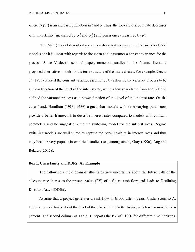
Box 1. Uncertainty and DDRs: An Example
The following simple example illustrates how uncertainty about the future path of the
discount rate increases the present value (PV) of a future cash-flow and leads to Declining
Discount Rates (DDRs).
Assume that a project generates a cash-flow of €1000 after t years. Under scenario A,
there is no uncertainty about the level of the discount rate in the future, which we assume to be 4
percent. The second column of Table B1 reports the PV of €1000 for different time horizons.
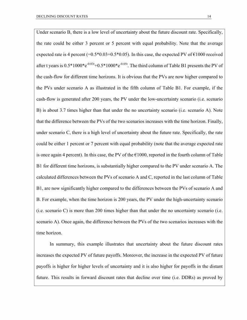
DECLINING DISCOUNT RATES 14
Under scenario B, there is a low level of uncertainty about the future discount rate. Specifically,
the rate could be either 3 percent or 5 percent with equal probability. Note that the average
expected rate is 4 percent (=0.5*0.03+0.5*0.05). In this case, the expected PV of €1000 received
after t years is 0.5*1000*e-0.03t+0.5*1000*e-0.05t. The third column of Table B1 presents the PV of
the cash-flow for different time horizons. It is obvious that the PVs are now higher compared to
the PVs under scenario A as illustrated in the fifth column of Table B1. For example, if the
cash-flow is generated after 200 years, the PV under the low-uncertainty scenario (i.e. scenario
B) is about 3.7 times higher than that under the no uncertainty scenario (i.e. scenario A). Note
that the difference between the PVs of the two scenarios increases with the time horizon. Finally,
under scenario C, there is a high level of uncertainty about the future rate. Specifically, the rate
could be either 1 percent or 7 percent with equal probability (note that the average expected rate
is once again 4 percent). In this case, the PV of the €1000, reported in the fourth column of Table
B1 for different time horizons, is substantially higher compared to the PV under scenario A. The
calculated differences between the PVs of scenario A and C, reported in the last column of Table
B1, are now significantly higher compared to the differences between the PVs of scenario A and
B. For example, when the time horizon is 200 years, the PV under the high-uncertainty scenario
(i.e. scenario C) is more than 200 times higher than that under the no uncertainty scenario (i.e.
scenario A). Once again, the difference between the PVs of the two scenarios increases with the
time horizon.
In summary, this example illustrates that uncertainty about the future discount rates
increases the expected PV of future payoffs. Moreover, the increase in the expected PV of future
payoffs is higher for higher levels of uncertainty and it is also higher for payoffs in the distant
future. This results in forward discount rates that decline over time (i.e. DDRs) as proved by
DECLINING DISCOUNT RATES 15
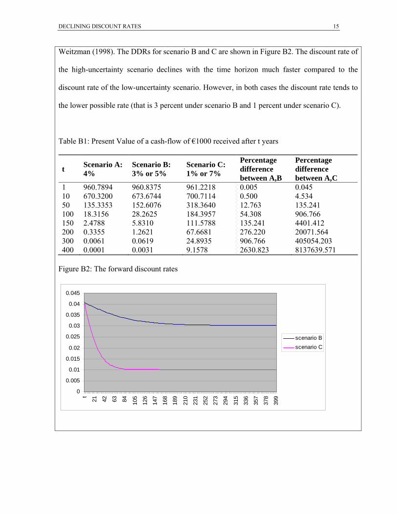
Weitzman (1998). The DDRs for scenario B and C are shown in Figure B2. The discount rate of
the high-uncertainty scenario declines with the time horizon much faster compared to the
discount rate of the low-uncertainty scenario. However, in both cases the discount rate tends to
the lower possible rate (that is 3 percent under scenario B and 1 percent under scenario C).
Table B1: Present Value of a cash-flow of €1000 received after t years
t Scenario A: 4%
Scenario B: 3% or 5%
Scenario C: 1% or 7%
Percentage difference between A,B
Percentage difference between A,C
1 960.7894 960.8375 961.2218 0.005 0.045 10 670.3200 673.6744 700.7114 0.500 4.534 50 135.3353 152.6076 318.3640 12.763 135.241 100 18.3156 28.2625 184.3957 54.308 906.766 150 2.4788 5.8310 111.5788 135.241 4401.412 200 0.3355 1.2621 67.6681 276.220 20071.564 300 0.0061 0.0619 24.8935 906.766 405054.203 400 0.0001 0.0031 9.1578 2630.823 8137639.571
Figure B2: The forward discount rates
0
0.005
0.01
0.015
0.02
0.025
0.03
0.035
0.04
0.045
t
21 42 63 84 105
126
147
168
189
210
231
252
273
294
315
336
357
378
399
scenario Bscenario C
DECLINING DISCOUNT RATES 16
2.3 Linking the Two Approaches of DDRs
In a frictionless economy, it is irrelevant to know whether the new marginal
investment project would be financed by a reduction in current consumption, or by a
reallocation of capital, since the equilibrium interest rates equals the return on capital and
the marginal rate of intertemporal substitution. Applying the extended Ramsey rule for a
one-year horizon, we obtain that the equilibrium interest rate must equal
21 1 0.5 (1 ) ,gδ ρ μ μ μ σ= + − +
where g1 is the expected growth rate and σ2 is the variance of the growth rate of
consumption. This means that there is a direct link between shocks on expectations about
the growth of the economy, and shocks on the short-term interest rate.
We have made clear in the previous sections that it is the persistency of the shocks
on the growth rate of consumption (in the consumption-based approach) and of the shocks
on short-term interest rates (in the production-based approach) which determines the shape
of the term structure of the socially efficient discount rate. The above equation shows that
these two explanations are coherent with each others. Persistent shocks on growth
expectations translate into persistent shocks on interest rates, both yielding DDRs.
In this paper, we use the production-based approach to DDRs. We have collected
data to test for the persistence of shocks on interest rates, and we use equation (2) to
characterize the term structure.
In reality, the two approaches are not perfectly equivalent in the real world.
Distortionary income taxation alone will cause the return on capital to be larger than the
marginal rate of intertemporal substitution. Imperfect competition, externalities in
DECLINING DISCOUNT RATES 17
production and consumption, differences in the value of investment and consumption etc.
will also cause a divergence. All of these factors require consideration in any given
circumstance when conducting CBA. Much of the debate about discounting has concerned
when and whether it is appropriate to use the consumption-based approach or the
production-based approach, or some combination of the two. Furthermore, the specific
Social Discount Rate (SDR) used for CBA will reflect the numeraire against which all
costs and benefits are valued. Most commonly in CBA consumption is used as the
numeraire, and thus δ is often referred to as the ‘consumption rate of interest’. Changing
the numeraire will change the level of the SDR, but will not change the outcome of the
NPV rule.
2.4 Time Inconsistency
It has been clear since at least Strotz (1956) that the myopic use of non-constant
discount rates results in time inconsistent plans. Dynamic inconsistency, or equivalently
‘time inconsistency’, arises when a plan determined to be optimal at a particular point in
time is not optimal when considered at a later point in time. In this case, if the planner is
unable to somehow commit future planners to the original plan, the plan will eventually be
abandoned.
Equating non-constant discount rates with time-inconsistent behaviour is a
fallacious interpretation of the literature. Let us make clear that an exponential discounting
of future utility, which implies time-consistency, is compatible with a non-exponential
discounting of future monetary flows, i.e., with a non-flat term structure of discount rates.
To show this, consider the 3-period consumption-saving problem under certainty:

DECLINING DISCOUNT RATES 18
1 2
0 1 2
1 2
2, , 0 1 2
20 1 2
max ( ) ( ) ( )
. . ,c c c u c e u c e u c
s t c e c e c w
ρ ρ
δ δ
− −
− −
+ +
+ + =
where ρt is the per-period rate of impatience associated to time-horizon t, δt is the interest
rate at date 0 of a zero-coupon bond with maturity at date t, and w is the lifetime wealth of
the agent. Exponential (utility) discounting holds only if ρ1=ρ2, and the term structure of
(monetary) discount rates is flat if δ1=δ2. The first-order conditions are written as
(3) 1 1 2 22 20 1'( ) '( ) '( ),u c e u c e u cδ ρ δ ρλ − −= = = 2
which yields a single optimal consumption plan when combined with the
budget constraint. Observe also that equations (3) are equivalent to the pricing formula
obtained when using the consumption-based approach in the certainty context.
* * *0 1 2( , , )c c c
Let time pass, and consider the decision problem of the same agent at date t=1. Is
the remaining consumption plan still optimal in the new context? The decision
problem can now be written as
* *1 2( , )c c
1
1 2
1
, 1 2
ˆ *1 2 1
max ( ) ( )
. . ( ),
c c u c e u c
s t c e c e w c
ρ
δδ
−
−
+
+ = −
where δ̂ is the short-term interest rate that prevails at date t=1. By a simple arbitrage
argument, it can be checked that 2ˆ 2 1δ δ δ= − . The first-order conditions for this problem
can be written as
(4) 1ˆ
1ˆ '( ) '( ).u c e u cδ ρλ −= = 2
1The two right equalities in (3) and (4) are compatible only if 1δ ρ− equals
2 2ˆ2 2 1δ ρ δ ρ− − + , which is true only if 1ρ equals 2ρ , that is, only if utility discounting is
exponential. Whether the term structure of (monetary) discount rates is flat, decreasing or
DECLINING DISCOUNT RATES 19
increasing is irrelevant for the time consistency of individual and collective decisions.
Agents are perfectly able to plan their future consumption levels with perfect foresight
about the evolution of their expectations and of interest rates. On the contrary, the relative
weight of utils at calendar date t and t+1 must remain constant through time in order to get
time consistent decisions.
A similar point can be made in an uncertain environment. In such an environment,
the optimal consumption plan is state-dependent. It is time consistent if agents do not want
to revise these state-contingent plans when time passes, and when uncertainty is
progressively resolved. As in the certainty case, it requires exponential discounting, but it
is fully compatible with a non-flat term structure.
3. FROM THEORY TO PRACTICE: THE EMPIRICAL ESTIMATION OF THE
OPTIMAL TRAJECTORY OF DDR
The discussion in Section 2 brings to light some interesting issues concerning the
characterization of the future path of interest rates. In the consumption-based approach, it
is mainly persistence of shocks on consumption growth that leads to decline in discount
rates over time. Similarly, persistence on shocks on interest rates is the force that generates
DDRs in the production-based approach. However, the existence of persistence is an
empirical question. This section shows how we can empirically estimate a schedule of
DDRs based on available historical data. Our objective is to calculate a sequence of an
aggregate DDR required for the case study examined in Section 4.
It should be clear by now that, in general, there are two different classes of models
to describe the behavior of the term structure of the social discount rate. That is, structural
DECLINING DISCOUNT RATES 20
models where forward rates are determined by exogenous variables (e.g. growth of
consumption) and univariate time series models where forward rates are determined by
past rates. The choice between the two approaches is not straightforward, since they both
have advantages and disadvantages.
From a theoretical point of view, a structural model is able to represent the
underlying economic relations and seems preferable to a simple univariate model. It is
reasonable to believe that if the assumptions underlying a structural model are valid, it will
produce better forecasts for the interest rate compared to a univariate model.
However, from an empirical point of view, the theoretical advantage of a structural
model over a univariate one can turn into a disadvantage if any of the assumptions of the
structural model is violated. On the other hand, the main assumption behind the univariate
model is that past behaviour of interest rates can reveal useful information about the future
dynamics of the series. Moreover, in the context of structural models, we need long-term
forecasts of all the variables that determine the interest rates in order to calculate the
projected values of the interest rates. This can create estimation problems due to the
possible time-variation of the parameters of the model. Furthermore, the researcher is
obliged to perform the analysis based on the period where data for all variables of the
structural model are available. This can result in the loss of important information. On the
other hand, a univariate model requires data only for the interest rate and thus the analysis
is usually extended to longer periods. It is reasonable to expect that when the objective is to
derive a schedule of discount rates for, say, the next 400 years, a model that is based on
150-200 years of data (i.e. information) will probably outperform a model that is based on,
say, only 60-80 years of data. The data availability issue is very important in our case
DECLINING DISCOUNT RATES 21
where we try to calculate an aggregate DDR based on a number of country-specific
estimates.
In summary, we believe that structural models are well-suited for short-term
forecasts. However, their empirical implementation to describe the behaviour of the term
structure in the distant future creates a number of problems described above. Therefore, we
choose to describe the behavior of interest rates in the context of univariate time-series
models. The utilization of a univariate model allows us to extend the estimation sample
using long historical data that cover more than 200 years in some cases. This allows us to
capture many historical events that affect the stochastic characteristics of the interest rate
series.
Our focus is on the determination of the stochastic nature of interest rates through
the observed dynamics of the process. After a short description of the available dataset, we
choose the optimal model to describe the real interest rate of the countries under scrutiny,
that is, France, India, Japan and South Africa. We then generate a series of discount factors
and DDRs for each country based on the simulation procedure introduced by Newel and
Pizer (2003). In a similar manner, we also generate discount factors and DDRs for
Australia, Canada, Germany, the UK and the US based on each country's optimal estimated
model as suggested by Hepburn et al. (2008) for the first four countries and Groom et al.
(2007) for the US.4 Afterwards, we construct the aggregate discount factor (and the
4In their simulation experiment, Hepburn et al. (2008) and Groom et al. (2007) set the initial value of the DDR equal to 3.5 and 4 percent, respectively. In this study, we set the initial value of the DDR equal to the sample mean. We therefore repeat the simulations for Australia, Canada, Germany, the UK and the US setting the initial value of the DDR equal to the sample mean in order to obtain a uniform set of results.
DECLINING DISCOUNT RATES 22
corresponding aggregate DDR) as a weighted average rate of the nine discount factors of
the individual countries.
3.1 Data
Social discount factors are prices of future consumption relative to consumption
today. The relative price of future consumption could be calculated from the risk-free
long-term interest rates. However, there are at least four arguments for the
inappropriateness of simply using market prices: (a) market imperfections, (b) the
super-responsibility of the government to both current and future generations, (c) the dual
role of the members of the present generation in that in their political role they may be
more concerned about future generations than their day-to-day activities on current
markets would reveal, and (d) Sen's (1982) argument that individuals may be willing to
join in a collective savings contract, even though they are unwilling to save as much in
isolation. Although some of these positions generated heated argument, the overall view
emerged that the real risk-free market interest rates provide an inappropriate conceptual
basis for social discounting. However, the alternative of using the shadow price on capital
in order to convert the magnitude of future effects to their consumption equivalents, is not
currently used by policy makers, reflecting a mix of practicability and the view that the real
risk-free interest rate and the shadow discount rate are quite close in magnitude
(Spackman, 1991; Arrow, 1995; Pearce and Ulph, 1999). Based on these results, we use
data on market interest rates for our empirical estimation.
We consider the real interest rate for France, India, Japan and South Africa. In an
attempt to use the longest possible interest rate series, we choose the 10-year Government
DECLINING DISCOUNT RATES 23
Bond Yield for France, the 7- and 20-year Government Bond Yields for Japan and South
Africa respectively and the Government Bond Yield for India (as constructed by Global
Financial Data). All interest rates are in domestic currency. Table 1 provided more
information about the available sample and the series under scrutiny. We first calculate the
real interest rate by subtracting the inflation rate (calculated based on the Consumer Price
Index). Similarly to Newel and Pizer (2003), we assume that the inflation rate is zero
before 1950. In order to preclude negative real interest rates from the analysis, we remove
the effect of short periods of unusually high inflation (e.g. during the oil crisis in the mid
'70s) using a simple dummy variable regression to subtract the extra level of inflation
observed during that periods. This approach is followed for all countries except India. In
the case of India, inflation is very high and volatile during the last 20 years, reaching 90
percent in some cases. Therefore, in the case of India and for the post-1973 period, we set
the inflation rate equal to the average inflation rate during the pre-1973 period. In all cases,
we consider a 4-year moving average real interest rate to smooth any short-term
fluctuations. We then convert the real interest rate series to their continuously compounded
equivalents. Finally, the estimation is based on the natural logarithm of the series to ensure
that the simulated DDRs are positive. We should note that negative discount rates are
unusual but not inconceivable. We choose to preclude negative discount rates for two
reasons. First, we want to be consistent with previous studies, such as Groom et al. (2007),
since we use some of their estimation results in our analysis. Second, we believe that
negative rates are unlikely to persist for long periods.
DECLINING DISCOUNT RATES 24
The basic descriptive statistics of the transformed series used in the estimation
procedure are reported in Table 2. The French rate has the higher mean, while the Japanese
rate is the more volatile one.
Table 1 here
Table 2 here
3.2 Country-specific DDRs
The aim of this section is to describe the statistical properties of the time path of the
interest rates. There are numerous studies in the literature which argue that interest rates are
subject to infrequent but important changes in the mean and the variance. The sources of
these structural changes are not clear but are probably related to either monetary or fiscal
policy. Moreover, the poor performance of various models (such as the Cox et al. (1985)
model) in empirical studies to describe the yield curve may be attributed to the fact that
they do not account for structural changes in the behavior of the interest rate. It is therefore
important to choose a model for the interest rate that takes into account the existence of
such structural changes, which is an important characteristic of the series. As a result, many
researchers have chosen regime-switching models to describe either a single time series of
an interest rate (e.g. Hamilton 1988 and Gray 1996) or the entire term structure of interest
rates (e.g. Bansal and Zhou, 2001). We follow a similar procedure and choose a
two-regime model to describe each interest rate series. Each one of the two regimes has a
different mean as well as a different variance. The level of persistence of the process under
each regime is also different. Finally, our specification allows for different lag order
specification between regimes and countries. In summary, our parameterization describes a
DECLINING DISCOUNT RATES 25
process that incurs a number of regime shifts over time where each regime has a different
mean, variance and persistence. We can also estimate the average time that the process
spends in each regime, which also determines the frequency of regime switches. Although
we are not certain about the regime of the process in each point in time, we can easily
estimate the probability of being in each regime over the sample period. The estimation
results and the model selection procedure are described in more detail in Appendix A.
We then implement a simulation methodology to generate a series of discount
factors (and the corresponding discount rates) for each country under examination. The
simulation uses each estimated model to simulate 200.000 possible future paths of the
interest rate. The simulation is structured so that it takes into account two different sources
of uncertainty that characterize the estimated model. First, the simulation considers the
typical uncertainty found in all stochastic models stemming from the stochastic nature of
the error term. In other words, random draws of the error terms are generated for each
simulated path. Second, the simulation accounts for the uncertainty that surrounds the
point estimates of the parameters of the regime-switching model. Specifically, each
simulated path of the discount rate uses a random draw for all the parameters of the model
based on the point estimates and the estimated variance-covariance matrix of the
parameters. The utilization of a two-regime model instead of a single-regime one allows
for the possibility of regime switches in the future. In other words, irrespectively of the
regime of the process during the recent years, the Regime-Switching (RS) model (and the
simulation exercise) considers the possibility that the process incurs a number of regime
changes in the future. This is crucial since we know that the calculated DDR depends on
the level of uncertainty and thus the estimated model used in the simulation should be able
DECLINING DISCOUNT RATES 26
to provide a relative good approximation of the actual uncertainty that surrounds the
behavior of the discount rates. For each simulated series, we set the initial values equal to
the sample mean of the real interest rate.5 One can reasonably argue that the long-period
average is not an appropriate initial value for the simulation exercise, since it generates an
initial value of the real interest rates that is higher than the real interest rates observed
during the recent years in some developed countries. In order to examine the sensitivity of
our results to the choice of the initial value in the simulations, at a later stage of our analysis
we repeat the simulations setting the initial rate equal to 3.5 percent (that is, the rate
currently used by HM Treasury for the evaluation of long-term projects). For the moment,
we focus on estimated discount factors for the case where the initial values equal the
sample mean of the series under examination.
The estimated discount factors and discount rates are reported in the first part of
Tables 3 and 4, respectively. In general, we observe significant differences in the discount
rates. France seems to produce the sharpest declining rate. Although the French one-period
ahead rate is substantially higher than that of the other three countries, its terminal value
(1.064 percent) is close to that of the Indian rate (0.858 percent) and lower than the
terminal rates of Japan and South Africa (1.39 and 2.358 percent respectively). On the
other hand, the interest rate of South Africa declines very slowly, by only 1.5 percent in
400 years. The differences between the speed of decline in the country-specific discount
rates mainly stems from the level of persistence of the individual series. The theoretical
results presented in Section 2 show that (in an uncertain environment) it is persistence that
leads to DDRs. The level of persistence determines the speed of decline in the forward
5See Groom et al. (2007) for further details about the design of the simulations.
DECLINING DISCOUNT RATES 27
discount rates. In our case, the French interest rate is the more persistent one and thus it
produces the sharpest DDR. On the other hand, the South-African interest rate is much less
persistent than the other three rates under scrutiny, resulting in a slowly declining forward
discount rate.
Table 3 here
Table 4 here
Tables 3 and 4 also report the estimated discount factors and rates for Australia,
Canada, Germany, the UK and the US based on each country's estimated model as
suggested by Hepburn et al. (2008) for the first four countries and Groom et al. (2007) for
the US. We repeated the simulations of the two aforementioned studies by using a different
initial value for the simulations. Specifically, we set the initial value equal to the sample
mean. By doing so, we end up with a uniform set of nine DDRs.6
3.3 Aggregation of the Discount Factors
Environmental degradation is one of the most important issues that affect the globe.
Growing international environmental interdependence and increased environmental
awareness over the past years led to multilateral efforts to promote international policies
and projects to mitigate problems like global warming and air pollution. The evaluation of
such multinational projects requires the calculation of a proper “global” discount rate. We
now try to compose such a discount rate. Specifically, we use the nine discount factor
series calculated above to construct a weighted average discount factor profile (and the
corresponding DDR profile) that can be used in cost-benefit analysis of long-term projects
6We should note that contrary to our sample that extends up to 2006, the estimation sample used by Hepburn et al. (2008) for Australia, Canada, Germany and the UK ends in 2004. Moreover, the estimation sample of
DECLINING DISCOUNT RATES 28
that affect the global environment and economy. On the other hand, when evaluating
projects that affect a single country, the cost-benefit analysis should be based on the
country-specific discount factors (like the ones reported in Table 3 of our study). We
believe that the aggregate discount factor profile is useful (and probably better than the
discount factors of any individual country) when evaluating projects that have a global
effect (e.g. climate change). The use of this aggregate interest rate is based on the
anticipation of a better international cooperation to harmonise policies relating to the
challenges raised by global changes to our planet.7
We consider three alternative weighting schemes in aggregating the
country-specific discount factors. The first weighting scheme is based on the GDP of each
country measured in Purchasing Power Parity terms. Specifically, the weight for each
country equals the ratio of its GDP over the sum of the GDP of all nine countries under
consideration. The second weighting scheme is based on annual CO2 emissions, that is, the
weight of each country equals the ratio of its annual CO2 emissions over the total annual
CO2 emissions of all nine countries of our sample. The third weighting scheme is based on
the population size of each country in 2005, that is, each country’s weight equals the ratio
of its population over the total population of all nine countries under examination.
Obviously, the first weighting scheme is more meaningful than the other two from an
economic point of view. On the other hand, we consider the three weighting scheme to be
meaningful in environmental terms and thus our analysis is based on all three alternative
weights for comparison reasons. Interestingly, the GDP and CO2 weights are similar
Groom et al. (2007) for the US ends in 1999. 7 We calculate the aggregate DDR based on a sample of only nine countries. Obviously, we would have been able to estimate a “better” DDR (i.e. more representative of the global DDR) if additional large countries (e.g.
DECLINING DISCOUNT RATES 29
resulting in similar aggregate discount factors and aggregate DDRs. Therefore, for brevity,
the rest of the discussion is limited to the discount factors and DDRs calculated based on
either the GDP or population weighting schemes.8 The two alternative weighting schemes
are reported in Table 5. We should also note that the nine countries under examination
correspond to about 46.8 percent of the world's GDP and about 28.34 percent of the world's
population.
Table 5 here
The weighted average DDRs for the two alternative weighting schemes, presented
in Table 6, have some differences but are in general close to each other. In general, the
population-based aggregate rate is higher than the GDP-based aggregate rate for the first
300 years, becoming lower than the GDP-based aggregate rate for the last 100 years of the
simulation. As a result, the terminal rate of the population-based aggregate rate is about 1.1
percent, that is, approximately 0.28 percent lower than that of the terminal GDP-based
aggregate rate (which is about 1.38 percent).
Table 6 here
The results presented in Section 4 show that the two alternative weighting schemes
generate quite similar valuations of climate change damages. In any case, we consider the
GDP-based aggregate rate more reliable than the population-based aggregate rates for at
least three reasons. First, GDP weights make more sense from an economic point of view.
This is why the majority of empirical studies that compose an aggregate interest rate use
weights based on GDP and the European Central Bank (ECB) calculates aggregate
Brazil, China and the Russian Federation) had been included in the analysis. Unfortunately, there are no reliable long historical data of interest rates series available for any of these countries.
DECLINING DISCOUNT RATES 30
measures for the EU based on each member’s GDP weight. Second, the nine countries
under scrutiny account for about 46.8 percent of the world's GDP and about 28.34 percent
of the world's population. Thus, the GDP-based aggregate rate seems to be more
representative of the global DDR than the population-based aggregate rate.9 Third, in the
context of our study, the behaviour of the population-based aggregate rate is mostly
defined by the dynamics of the Indian rate, since the population-based weight for India is
above 60 percent.
4. DISCOUNTING CLIMATE CHANGE DAMAGES
There are many uncertainties when it comes to the climate. There are uncertainties
related to cloud formation, feedback from methane in melting permafrost and ecosystem
responses to rapid change, to mention just a few. Hence it may come as a surprise to some
non-economists that the main source of uncertainty in estimates of the economic
consequences of climate change is something else: the discount rate. In fact, much of the
critique of the Stern Review has focused not on the climate science embodied in the report
or its assessment of the costs and benefits of climate change mitigation, but on the low
discount rate used in the analysis and how this drives the central results of the Review (see
e.g., Dasgupta (2006), Yohe (2006), Nordhaus (2007), Weitzman (2007a)). In this section,
we investigate the policy implications of applying the two weighted average discount
factors (and the corresponding DDRs) calculated in the previous section, on the
8 We also used an alternative weighting scheme, which is based on the projected population of each country in 2050. As expected, the results of this weighting scheme were similar to those based on each country’s population in 2005 and are not reported for brevity. 9 The fact that the aggregate DDR calculated based on the CO2-emissions weights (not reported for brevity) produces similar results to the GDP-based DDR reinforces our belief that the GDP-based DDR seems to be a better approximation to the “global DDR”.
DECLINING DISCOUNT RATES 31
cost-benefit evaluation of the carbon mitigation policies and the conclusions of the Stern
report.
4.1 The Discount Rate in the Stern Review
The Stern Review contains a very careful and nuanced discussion of the discount
issue (Stern, 2006, chapter 2). Under the assumption of a Constant Elasticity of
Substitution (CES) utility function for consumption, the choice of the discount rate in the
Review is based on the Ramsey equation ( gδ ρ μ= + ) where δ is the discount rate, μ is
the elasticity of the marginal utility of consumption, g is the growth rate of consumption
(which is time varying) and ρ is the pure time discount rate or the rate of time preference.
Since the growth rate is eventually depressed by climate change, the consumption discount
rate falls through time. Moreover, because a small number of Monte Carlo draws simulate
severe damages and therefore low growth, the certainty-equivalent falls towards the
trajectory of the lowest rate (highest damages). This should be analogous to what happens
in a schedule of time-declining discount rates based on past, exogenous volatility in
growth.
However, the Review assumes that the elasticity of marginal utility is 1μ = ,
implying that the utility function is logarithmic. To accommodate for the fact that future
generations will be richer, the growth effect to the discount rate is accounted for by
assuming that the average annual rate of growth of consumption is 1.3% (Review, Box 6.3).
Moreover, the Review argues that on ethical grounds the welfare of future generations
should be treated at par with the welfare of the present generation, a position that implies
the selection of a zero pure time discount rate. However, the Review also claims that
DECLINING DISCOUNT RATES 32
uncertainty for the existence of the human race suggests that a positive rate should be
selected instead (Review, Technical Annex to Postscript). Thus, the pure time discount rate
is set at 0.1%, meaning that the survival probability of the human race for 100 years is 0.91.
The Review acknowledges that there exist justifications for using higher pure time
discount rates that suggest that pure time discount rate can be thought of as covering the
possibility of reversing a particular investment. However these justifications are invalid in
the case of climate change cost evaluation since “climate change is long-term, severe and
irreversible”. This is the reason why the justification that technological or other advances
may mitigate climate change in the future, is not employed. In addition, it is supposed that
future generations would willingly exchange conventional capital stock with improved
environmental conditions in the future. As a result, the overall discount rate that is derived
from the average growth of 1.3% is 1.4%, which is an unusually low value!
This low discount rate is entirely consistent with the Ramsey rule, but it crucially
depends on the chosen values for the structural parameters. If a researcher chooses a
different value for any of these parameters, the calculated discount rate will be
substantially different than 1.4 percent and as a result the CBA will probably lead to
different conclusions. For example, with μ=2, the socially efficient discount rate would be
2.7 percent. The discounting approach used in the Review and the chosen values for the
structural parameters has been the subject of much controversy and criticism (see, for
example, Dasgupta, 2006; Nordhaus, 2007).
DECLINING DISCOUNT RATES 33
4.2 The Social Cost of Carbon
The social cost of carbon (SCC) is the shadow price of anthropogenic carbon
dioxide emissions. The SCC is defined as the present value of the stream of damages from
one ton of carbon. In this section the results of the two weighted average DDRs calculated
in the previous section are applied to the calculation of the SCC. The SCC for each of the
weighted discounting profiles is calculated based on the baseline damages scenario of the
FUND 2.8 integrated assessment model, which reports the projected cost of emissions in $
per ton of carbon emissions (Tol 2002a, 2002b). This model estimates the impacts of
climate change to a wide variety of market and non market sectors like agriculture, forestry,
sea-level rise, ecosystems, fatal vector-borne diseases, and fatal cardiovascular and
respiratory disorders. The results represent the aggregation of the effects of climate change
in 9 different regions: OECD-America (excl. Mexico), OECD-Europe, OECD-Pacific
(excl. South Korea), Central and Eastern Europe and the former Soviet Union, Middle
East, Latin America, South and Southeast Asia, Centrally Planned Asia, and Africa. The
parameters used in the analysis are derived from the relevant literature. The results indicate
that climate change will have different implications according to the region and the sector
examined.
In Panel A of Table 7 we present the implied SCC using the GDP and 2005
population weighted profiles. In addition to the SCC calculated based on the estimated
average discount factors (second column of Table 7 labeled “Average”), we also report
lower and upper bounds for the SCC. More in detail, the lower bound corresponds to the
SCC calculated based on the lower 2.5 percent quantile of the simulated distribution of the
discount factors, while the upper bound corresponds to the SCC calculated based on the
DECLINING DISCOUNT RATES 34
upper 97.5 percent quantile of the simulated distribution of the discount factors.10 Table 7
also reports the social cost of carbon under a constant discounting regime of 1.4% per year
approximating the one implemented in the Stern Review. As a measure of comparison, the
US Environmental Protection Agency estimates that the average 2-person household in the
US produces approximately 20 tons of CO2 annually.11
Table 7 here
The social cost of carbon under GDP weighting is 12.60$/tonC. When using population
weighting, the overall social cost of carbon decreases by 29.76% to 8.85$/tonC. Under the
constant 1.4% rate, the social cost of carbon is 40.15$/tonC. These results are indicative of
the significance of discounting assumptions to the long-term valuation of climate change.
Using a low albeit constant discount rate (1.4%) increases the valuation of social benefits
from CO2 abatement from 3.18 to 4.5 times than under declining discounting patterns. We
now turn to the estimated 95 percent confidence intervals for the SCC that reveal the
uncertainty that surrounds the calculated SCC. Specifically, under a scenario of high
discount rates, the calculated SCC is as low as 3.09$/tonC and 2.48$/tonC for the GDP
weighted and population weighted discount factors respectively. On the other hand, under
a low discount rate scenario, the SCC increases to 23.69$/tonC and 17.99$/tonC for the
GDP weighted and population weighted discount factors respectively. We should note
however that in all cases the calculated SCC under the DDRs is substantially lower than
that under the 1.4 percent constant discount rate.
As mentioned earlier in this study, it is interesting to examine the sensitivity of our
results to the choice of the initial value in the simulation exercise that estimates the
10 Due to computational limitations, we use 50.000 replications to obtain the upper and lower bounds. 11 http://www.epa.gov/climatechange/emissions/ind_calculator.html.
DECLINING DISCOUNT RATES 35
discount factors and rates. Therefore, we repeat the simulations setting the initial rate equal
to 3.5 percent.12 Panel B of Table 7, reports the SCC estimated from GDP and Population
weighted discount profiles given a 3.5 percent initial rate. The implied results are slightly
higher compared to the original weighted discount schemes but still substantially lower
compared to the constant 1.4% rate. We, thus, observe that setting a different initial value
in the simulation exercise results in similar estimated SCC.
Figure 1 illustrates the evolution of benefits from a reduction of one ton in CO2
emissions over time for the GDP, population, GDP and Population with a 3.5% initial
value weighted schemes as well as for the 1.4% constant discount rates.
Figure 1 here
Figure 1 reveals that the majority of the benefits from reducing emissions by one
ton of CO2 under both weighting schemes are accumulated until the year 2200. Between
the year 2200 and 2400 the discounted benefits are of substantially smaller magnitude.
Benefits under the two weighting profiles are consistently lower when compared to the
constant 1.4% discounting profile. The benefits under GDP weighting are higher compared
to the population weighting for the first 300 years, while this is reversed for the final 100
years. The utilization of a lower initial value of 3.5 percent has a minor effect on the
evolution of benefits. The oscillating pattern in the lines of Figure 1 is caused by the nature
of the damages assumed by the FUND 2.8 model. Specifically, damages from one ton of
CO2 are assumed to remain constant across decades while the discounting profile is a
yearly time series. Furthermore, the cost of carbon is greater in the short- and medium-term,
but fall as carbon becomes sequestrated in the medium-term, thus generating the hump
12 We should note that in cases where the mean value of the series (as suggested by the estimated model) is higher than 3.5 percent, setting the initial value to 3.5 percent results in a forward discount rate that initially
DECLINING DISCOUNT RATES 36
shape. In Table 8 we display the present value of the benefits from reducing emissions by
one ton at selected years while in Table 9 we report the marginal contribution to the present
value at these years. Both tables illustrate that the contribution to aggregate benefits
significantly flattens out after 150 years for both declining discount rate weights. On the
other hand, benefits from abatement under constant 1.4% discounting exhibit similar
noticeable flattening only after the 250th year.
Table 8 here
Table 9 here
In Table 10 we report the estimated average social cost of carbon and its 95 percent
confidence interval for each one of the nine countries under consideration. North American
countries exhibit the highest SCC, since for the US and Canada the estimated values are
18.39$/tonC (3.90$/tonC, 31.55$/tonC) and 11.65$/tonC (1.08$/tonC, 30.23$/tonC)
respectively. Australia has the next highest average SCC with 11.45$/tonC (4.92$/tonC,
20.96$/tonC). The two major European industrial countries represented in the sample the
UK and Germany cluster next with 9.40$/tonC (4.43$/tonC, 16.54$/tonC) and 8.67$/tonC
(1.88$/tonC, 19.89$/tonC) respectively. For Japan the SCC is 8.45$/tonC (2.69$/tonC,
17.39$/tonC) and for South Africa with 7.95$/tonC (3.07$/tonC, 16.05$/tonC). France and
India display roughly average identical SCC with 6.35$/tonC (1.35$/tonC, 16.18$/tonC)
and 6.46$/tonC (2.05$/tonC, 14.11$/tonC) respectively. It is worth noting the disparity
between the implied SCC among countries that is suggested from the different discount
rates applied. Indicatively, the implied SCC for the US is approximately three times the
one for France and India.
Table 10 here
increases for a short period (moving up towards the mean) before starting its declining movement.
DECLINING DISCOUNT RATES 37
Figure 2 graphically illustrates the evolution of benefits from abatement through
time for each of the countries in the sample. For all countries in the sample except the US,
contributions fall significantly after the 150th year. For example, the marginal contributions
are close to zero for South Africa, Japan, Germany and the UK after the 200th year. Counter
to this, the marginal benefits for the US remain noticeable until the 250th year.
Figure 2 here
4.3 Using the Baseline + Market Impact + Non-market Impact Damages Scenario of
the Stern Review
Our purpose is to compare the implications on the monetary valuation of the
damages from climate change from the two different models (FUND 2.8 and PAGE2002)
under different discounting regimes. In this section, we present the results implied from the
baseline + market + non market damages from the Stern Review. The baseline scenario in
the Stern Review is designed to be consistent with the Intergovernmental Panel on Climate
Change (IPCC) third assessment report and assumes a mean warming of 3.9oC relative to
pre-industrial levels by 2100. The IPCC’s third assessment report estimates a mean
temperature increase ranging from 1.5oC to 4.5oC.
The damages are estimated using the integrated assessment model employed by the
Review that combines scientific models of climate change and economic modelling of the
effects of climate change. As stated in the text the assumption of the Review is that climate
change depresses the growth rate. According to the Stern Review, the primary sources of
emissions in the future will be today’s developing nations and China is expected to account
for one third of the increase. The Review reports evidence that economic growth has lead
DECLINING DISCOUNT RATES 38
to decarbonisation of the rich developed economies through changes in the production
process, demand patterns and institutional changes. Nevertheless, it implies that we cannot
rely on this effect for facing climate change and policies limiting CO2 emissions are
required. Under a Business as Usual Scenario, CO2 emissions will continue to increase.
According to the simulations in the Review the largest component of CO2 emissions will
be a by-product of energy production. To break down CO2 emissions from energy
production to its constituent parts the Review employs the Kave identity according to
which:
CO2 emissions from energy=Population*GPD per Head*(Energy Use/GDP)*
(CO2 emissions/Energy Use)
Hence, an increase in global GDP is expected to increase emissions from energy unless
there are offsetting effects from the emissions intensity of energy use or the energy
intensity of GDP.
Damages from climate change as illustrated in the Stern Review are significantly
different in their format compared to those reported from the FUND 2.8 model. Damages
in the former are reported as monetary and percentage losses in per capita GDP relative to
the per capita GDP in the state of the world under no climate change. Since the Review
does not describe how the social cost of carbon is calculated and since it reports no series of
projected emissions it is not possible to calculate the SCC in this case. However, we can
derive the implications of the two discount factor weighting schemes to the overall
damages from climate change reported by the Review, as well as the implications for the
welfare of individual countries in the sample.
DECLINING DISCOUNT RATES 39
In order to be consistent with the previous section and in line with the estimated
discounting profiles we assume that all present values are reported as of 2005 for damages
occurring from 2006 onwards. Contrary to the Stern Review, in the calculations, we
assume that the horizon is 400 years instead of 200 years to account for the full length of
the discounting profile. Since the damages are reported in intervals, we assume that for
years within those intervals the decrease in GDP is equal to the damage for the interval.
The damages between the 200th and 400th year are assumed to be equal to those of the 200th
year while damages after the 400th year are ignored.
In Table 11 we report the present value of damages from climate change using
different discounting profiles (that is GDP weighting, Population weighting, constant 1.4
percent, as well as GDP and Population weighting based on a 3.5 percent initial value).
Damages from climate change are defined as the difference between the projected GDP per
capita under no climate change and under the baseline scenario in the Stern Review. The
results indicate that the present value of damages under the GDP weighting is
approximately twice the present value of damages under population weighting.
Specifically, over the 400 year horizon the average present value of damages per capita in
the baseline scenario is $10505.61 under GDP weighting while it is $5056.85 under
population weighting. Damages under the constant 1.4% regime greatly exceed the
declining rate regimes with the resulting present value being $76099. Given that the
estimate specified by the Stern Review for the mean per capita income in 2001 is $7240,
the present value of the damages calculated for the GDP weighting, population weighting
and the constant 1.4% profile are 1.45, 0.69 and 10.5 times the 2001 mean per capita
income respectively. Using an initial rate of 3.5% in the simulation exercise to estimate the
DECLINING DISCOUNT RATES 40
GDP and Population weighted discount profiles produces slightly higher damage estimates
compared to the original ones: the PV is 10832.79 and 5382.90 respectively.
Table 11 here
To evaluate the dynamic evolution of damages, we calculate the aggregate present
value of the difference between the no climate change scenario and the baseline scenario
for each year, under all the discount profiles. The results are reported in Table 12. It is
worth noting that for all discounting profiles, more than half of the value of per capita
damages from climate change, arises during the time period between years 200 to 400,
which is not accounted for in the Stern Review. This effect is greater for the
population-weighted discounting profile. Adopting a 200 year horizon suggests that the
present value of damages for the GDP, the Population and the constant 1.4% profiles are
$5559, $3014 and $29798, respectively. Furthermore, when using a 3.5 percent as an initial
value in the simulations, the relevant values for the GDP and Population weighted profiles
are $5762 and $3242 respectively. The evolution of the present value of damages over time
is also visualized in Figure 3. It is evident that the two alternative GDP-based discount
profiles (i.e. one calculated using the sample mean as an initial value and one calculated
using a 3.5 percent as an initial value) generate almost identical damages. The same holds
for the two alternative population-based discount profiles.
Table 12 here
Figure 3 here
As illustrated in Tables 11, 12 and Figure 3, the choice of the discounting profile
has significant impacts on the valuation of damages borne by climate change over the
specified 400 year horizon. Adopting either of the two weighted declining discounting
DECLINING DISCOUNT RATES 41
profiles, results to substantially lower estimates of climate change damages compared to
the ones derived in the Stern Review. This is attributed, to a large extent, to the small value
of the pure time discount rate that is assumed in the Review, in order to accommodate
damages across generations in an egalitarian fashion. Nevertheless, a declining discount
profile can correct the insufficient representation of future generations, but at the same
time better maintain that current generations discount the future.
The analysis also reveals that the calculated valuations of climate change damages
from the two alternative weighted discount profiles are of the same magnitude. However,
we observe that the GDP-based DDR produces slightly higher valuation of climate change
damages compared to the population-based DDR. This stems from the fact that the two
weighting schemes (and as a result the corresponding DDRs) are not similar with respect to
their ability to ‘represent’ the ‘global situation’. In terms of GDP, our sample represents
about 46.8 percent of the world's GDP. On the other hand, our sample represents only
28.34 percent of the world's population. As a result, the GDP-based DDR is clearly a better
approximation to the ‘global DDR’. We believe that the two aggregate DDRs would
become similar to each other if it was feasible to include additional large countries in the
analysis.
5. CONCLUDING REMARKS
Our main point in this paper is that when uncertainty is taken into account, the case for the
use of Declining Discount Rates (DDRs) in long-run cost-benefit analyses becomes
compelling. The decision to replace constant discount rates with DDRs has serious policy
implications. In fact, such a decision implies that the policy maker will put relatively more
DECLINING DISCOUNT RATES 42
effort to improve social welfare in the far distant future than in the shorter time. In this
paper we emphasize that the relative value of this effort cannot be decided arbitrarily. A
theory-consistent and empirically reliable estimation method is needed. To develop this
method, we assume a declining, but time-stable structure of discount rates, and connect the
representative-individual intergenerational theory with the empirical treatment of
country-specific historical data. The application of our method gives empirical estimates of
DDRs schedule. This estimated schedule is used for the calculation of a sequence of
aggregate (‘global’) DDR schedule, which is used for the CBA of climate change
mitigation policies. Our results add to the ‘discount rate-related’ criticism of the Stern
Review, that is, the results of the Review are driven by an arbitrarily low constant discount
rate. In conclusion, we claim that a DDR profile, if correctly estimated, can correct the
insufficient representation of future generations, but at the same time better maintain that
current generations discount the future.
One of the most important contributions of this paper is that it proposes how the
theory consistent optimal long-run trajectory of the decline in discount rates can be
efficiently estimated, without the use of a structural model. We believe that structural
models are well-suited for short-term forecasts. However, their empirical implementation
to describe the behaviour of the term structure of the interest rate in the distant future
creates a number of problems, which we have discussed in section 3. Our alternative
approach describes interest rates by means of a simple univariate time series model and is
based on the assumption that the past behavior of interest rates can reveal useful
information about the future dynamics of the series. Our model describes the uncertainty in
the behavior of interest rates. This uncertainty together with persistence of the interest rates
DECLINING DISCOUNT RATES 43
leads to DDRs. The utilization of a univariate model allows us to extend the estimation
sample using long historical data that cover more than 200 years in some cases. This allows
us to capture many historical events that affect the stochastic characteristics of the interest
rate series for the nine ‘representative’ countries we study. In particular, we use
regime-switching models to describe the stochastic dynamics of the real interest rate and
derive a schedule of DDR for each country under scrutiny.
We then compose two alternative weighted declining discounting profiles that can
be used in cost-benefit analyses of ‘global’ projects: the GDP-based DDR and the
population-based DDR. These two profiles are applied on the cost-benefit evaluation of
carbon mitigation policies and the conclusions of the Stern Report. We believe that this is a
very timely exercise, given that much of the critique of the Review has focused on the low
discount rate used in the analysis and how this drives the central results. Adopting either of
the two weighted declining discounting profiles, results to substantially lower estimates of
climate change damages compared to the ones derived in the Stern Review. This is
attributed, to a large extent, to the small value of the pure time discount rate that is assumed
in the Review, in order to accommodate damages across generations in an egalitarian
fashion. Our declining discount profiles correct the insufficient representation of future
generations, but at the same time better maintain that current generations discount the
future. We should note however that the estimated confidence intervals for the valuation of
carbon mitigation policies reveal the uncertainty that surrounds the calculated net present
values of climate change damages in cases where the (unknown) future discount rates are
very low or high.
DECLINING DISCOUNT RATES 44
In closing this paper we want to briefly mention possible future research directions.
Our methodology for the estimation of country-specific DDRs and the calculation of an
aggregate DDR is based on univariate specifications for the interest rates. Thus, our
empirical approach ignores the future stochastic consumption-growth process. The
theoretical work of Gollier (2007) and Weitzman (2007b) provides a promising route for
future investigation where consumption growth (and especially consumption growth-rate
volatility) and people’s preferences enter the analysis for the calculation of a DDR.
DECLINING DISCOUNT RATES 45
REFERENCES
Ang, A. and G. Bekaert (2002). ‘Regime Switches in Interest Rates’, Journal of
Business and Economic Statistics, 20, 163-182.
Arrow, K. J. (1995). ‘Economic Growth, Carrying Capacity, and the Environment’,
Ecological Economics, 15(2), 91-95.
Bansal, R. and H. Zhou (2002). ‘Term Structure of Interest Rates with Regime
Shifts’, The Journal of Finance, 57(5), 1997-2043.
Black, F., E. Derman and W. Toy (1990). ‘A One-factor Model of Interest Rates
and its Application to Treasury Bond Options’, Financial Analysts Journal, 46(1), 33-39.
Black, F. and P. Karasinski (1991). ‘Bond and Option Pricing when Short Rates are
Lognormal’, Financial Analysts Journal, 47(4), 52-59.
Chan, K.C., G.A. Karolyi, F.A. Longstaff and A.B. Sanders (1992). ‘An empirical
Comparison of Alternative Models of the Short-term Interest Rate’, Journal of Finance, 47,
1209–1227.
Cowell, F. and K. Gardiner (1999). ‘Welfare Weights’, Report to the UK Office of
Fair Trading (available at www.oft.gov.uk/NR/rdonlyres/).
Cox, J.C., J.E. Ingersoll and S.A. Ross (1985). ‘A Theory of the Term Structure of
Interest Rates’, Econometrica, 53, 385–407.
Dasgupta, P. (2006). ‘Comments on the Stern Review’s Economics of Climate
Change’, available from: http://www.econ.cam.ac.uk/faculty/dasgupta/STERN.pdf
DECLINING DISCOUNT RATES 46
Evans, D. and H. Sezer (2002). ‘A Time Preference Measure of the Social Discount
Rate for the UK’, Applied Economics, 34, 1925-34.
Gollier, C. (2002a). ‘Time Horizon and the Discount Rate’, Journal of Economic
Theory, 107(2), 463-73.
Gollier, C. (2002b). ‘Discounting an Uncertain Future’, Journal of Public
Economics, 85, 149-166.
Gollier, C. (2007). ‘The Consumption-Based Determinants of the Term Structure
of Discount Rates’, Mathematics and Financial Economics, forthcoming.
Gray, F.S. (1996). ‘Modelling the Conditional Distribution of Interest Rates as a
Regime-switching Process’, Journal of Financial Economics, 42, 27-62.
Groom, B., P. Koundouri, E. Panopoulou and T. Pantelidis (2007). ‘An
Econometric Approach to Estimating Long-Run Discount Rates’, Journal of Applied
Econometrics, 22, 641-656.
Hamilton, J.D. (1988). ‘Rational Expectations Econometric Analysis of Changes in
Regime: An Investigation of the Term Structure of Interest Rates’, Journal of Economic
Dynamics and Control, 12, 385-423.
Hamilton, J.D. (1989). ‘A New Approach to the Economic Analysis of
Nonstationary Time Series and the Business Cycle’, Econometrica, 57, 357-384.
DECLINING DISCOUNT RATES 47
Hepburn, C., P. Koundouri, E. Panopoulou and T. Pantelidis (2008). ‘Social
Discounting under Uncertainty: A Cross-country Comparison’, Journal of Environmental
Economics and Management, forthcoming.
Ho, T.S.Y. and S.B. Lee (1986). ‘Term Structure Movements and Pricing Interest
Rate Contingent Claims’, Journal of Finance, 41, 1011-1029.
Hull, J. and A. White (1990). ‘Pricing Interest Rate Derivative Securities’, Review
of Financial Studies, 3(4), 573-592.
Newell, R. and W. Pizer (2003). ‘Discounting the Benefits of Climate Change
Mitigation: How Much Do Uncertain Rates Increase Valuations?’, Journal of
Environmental Economics and Management, 46 (1), 52-71.
Nordhaus, W. D. (2007). ‘A Review of the Stern Review on the Economics of
Climate Change’, Journal of Economic Literature, 45(3), 686-702.
Pearce, D.W. and D. Ulph (1999). ‘A Social Discount rate for the United Kingdom’,
in Pearce, D.W., Environmental Economics: Essays in Ecological Economics and
Sustainable Development. Cheltenham: Edward Elgar, 268–285
Population Division of the Department of Economic and Social Affairs of the
United Nations Secretariat (2005). World Population Prospects: The 2004 Revision.
Highlights. New York: United Nations.
Ramsey, F.P. (1928). ‘A Mathematical Theory of Saving’, Economic Journal, 38,
543–59.
DECLINING DISCOUNT RATES 48
Sen, A.K. (1982). ‘Approaches to the Choice of Discount Rate for Social
Benefit-Cost Analysis’, in Lind, R.C. (ed) Discounting for Time and Risk in Energy Policy.
Washington, DC: Resources for the Future, 325-353.
Spackman, M. (1991). ‘Discount Rates and Rates of Return in the Public Sector:
Economic Issues’, GB HM Treasury.
Stern, N. (1977). ‘The Marginal Valuation of Income’, in Artis, M. and R. Nobay
(eds.), Studies in Modern Economic Analysis, Oxford: Blackwell.
Stern, N.H. (2006). ‘The Economics of Climate Change’, available at:
http://www.hm-treasury.gov.uk/independent_reviews/stern_review_economics_climate_
change/stern_review_report.cfm
Strotz, R. (1956). ‘Myopia and Inconsistency in Dynamic Utility Maximisation’,
Review of Economic Studies, 23, 165-180.
Tol, R.S.J. (2002a). ‘Estimates of the Damage Costs of Climate Change. Part 1:
Benchmark Estimates’, Environmental & Resource Economics, 21(1), 47-73.
Tol, R.S.J. (2002b). ‘Estimates of the Damage Costs of Climate Change, Part II.
Dynamic Estimates’, Environmental & Resource Economics, 21(2), 135-160.
Vasicek, O. (1977). ‘An Equilibrium Characterisation of the Term Structure’,
Journal of Financial Economics, 5, 177-188.
Weitzman, M. (1998). ‘Why the Far Distant Future Should be Discounted at its
Lowest Possible Rate’, Journal of Environmental Economics and Management, 36,
201-208.
DECLINING DISCOUNT RATES 49
Weitzman, M. (1999). ‘Just keep on discounting, but …. ‘, in Portney, P. and J.
Weyant (eds.), Discounting and Intergenerational Equity, Washington DC, Resources for
the Future, 23-30.
Weitzman, M.L. (2007a). ‘A Review of the Stern Review on the Economics of
Climate Change’, Journal of Economic Literature, 45(3), 703-724.
Weitzman, M.L. (2007b). ‘Subjective Expectations and Asset-Return Puzzles’,
American Economic Review, 97(4), 1102-1130.
Yohe, G. (2006). ‘Some Thoughts on the Damage Estimates Presented in the Stern
Review—An Editorial’, The Integrated Assessment Journal, 6(3), 65-72.
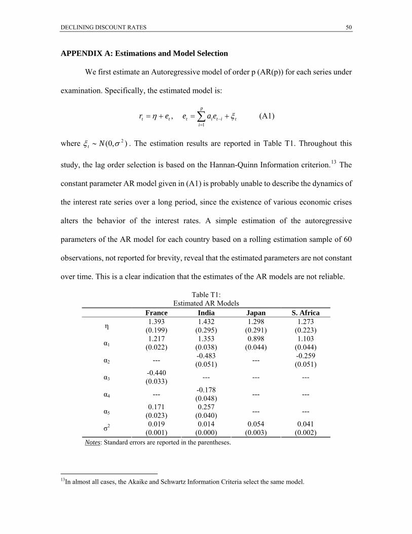
DECLINING DISCOUNT RATES 50
APPENDIX A: Estimations and Model Selection
We first estimate an Autoregressive model of order p (AR(p)) for each series under
examination. Specifically, the estimated model is:
titii
p
ttt eaeer ξη +=+= −=∑
1
, (A1)
where . The estimation results are reported in Table T1. Throughout this
study, the lag order selection is based on the Hannan-Quinn Information criterion.
),0( 2σξ Nt ∼
13 The
constant parameter AR model given in (A1) is probably unable to describe the dynamics of
the interest rate series over a long period, since the existence of various economic crises
alters the behavior of the interest rates. A simple estimation of the autoregressive
parameters of the AR model for each country based on a rolling estimation sample of 60
observations, not reported for brevity, reveal that the estimated parameters are not constant
over time. This is a clear indication that the estimates of the AR models are not reliable.
Table T1: Estimated AR Models
France India Japan S. Africa 1.393 1.432 1.298 1.273 η (0.199) (0.295) (0.291) (0.223) 1.217 1.353 0.898 1.103 α1 (0.022) (0.038) (0.044) (0.044)
-0.483 -0.259 α2 --- (0.051) --- (0.051) -0.440 α3 (0.033) --- --- ---
-0.178 α4 --- (0.048) --- ---
0.171 0.257 α5 (0.023) (0.040) --- ---
0.019 0.014 0.054 0.041 σ2 (0.001) (0.000) (0.003) (0.002)
Notes: Standard errors are reported in the parentheses.
13In almost all cases, the Akaike and Schwartz Information Criteria select the same model.
DECLINING DISCOUNT RATES 51
In the literature, there are various efforts to produce time-dependent models for the
interest rate, i.e. models with time-varying parameters.14 Since the seminal works of
Hamilton (1988, 1989), regime-switching (RS) models became a very popular class of
models to describe the time-variation in the dynamics of interest rates. In this study, we
consider the following two-regime model:
titki
i
p
ttkt eaeer ξη +=+= −=∑
1
, (A2)
where for the first and second regime respectively. We allow the
two regimes to have different lag order. This model allows the interest rate to have
different behavior in different periods by moving from one regime to the other. In regards
to the probability law governing the transition from the first regime to the second regime
and vice versa, we assume the simplest case of a Markov 1 chain, that is
),,0( 2kt N σξ ∼ 2,1=k
ijttttttt pisjsrrgsisjs ======= −−−−− )|(Pr,...),,...,,|(Pr 12121 (A3)
where . In other words, the probability of being in regime j at time t (2,1, =ji jst = )
depends on only the most recent regime ( ). 1−ts
The estimation results, reported in Table T2, show that the first regime corresponds
to periods of low real interest rates and high volatility, while the second regime
corresponds to periods of high real interest rates and low volatility. In all cases both
regimes are persistent as indicated by the estimated transition probabilities which are
always above 90 percent. In other words, the estimation results suggest that we do not
observe many regime switches during the period under scrutiny. This is illustrated in
14See, inter alia, Ho and Lee (1986), Black et al. (1990), Hull and White (1990) and Black and Karasinski (1991).
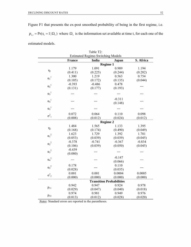
DECLINING DISCOUNT RATES 52
Figure F1 that presents the ex-post smoothed probability of being in the first regime, i.e.
where is the information set available at time t, for each one of the
estimated models.
)|1Pr(,1 ttt sp Ω== tΩ
Table T2: Estimated Regime-Switching Models
Notes: Standard errors are reported in the parentheses.
France India Japan S. Africa Regime 1
1.179 1.091 0.989 1.194 η1 (0.411) (0.225) (0.244) (0.282) 1.300 1.219 0.563 0.754 α1
1 (0.105) (0.172) (0.135) (0.044) -0.393 -0.486 0.478 α2
1 (0.131) (0.177) (0.193) ---
α31 --- --- --- ---
-0.311 α41 --- --- (0.148) ---
α51 --- --- --- ---
0.072 0.064 0.110 0.098 σ21 (0.008) (0.012) (0.024) (0.012)
Regime 2 1.484 1.565 1.133 1.395 η2 (0.168) (0.174) (0.490) (0.049) 1.623 1.729 1.392 1.781 α1
2 (0.053) (0.039) (0.039) (0.045) -0.378 -0.741 -0.367 -0.834 α2
2 (0.106) (0.039) (0.050) (0.045) -0.439 α3
2 (0.080) --- --- ---
-0.147 α42 --- --- (0.066) ---
0.178 0.110 α52
(0.028) --- (0.035) ---
0.001 0.001 0.0004 0.0005 σ22 (0.000) (0.000) (0.000) (0.000)
Transition Probabilities 0.942 0.947 0.924 0.978 p11 (0.029) (0.047) (0.040) (0.018) 0.974 0.981 0.949 0.976 p22 (0.013) (0.012) (0.028) (0.020)
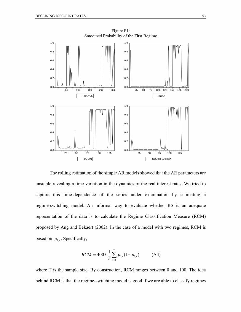
DECLINING DISCOUNT RATES 53
Figure F1: Smoothed Probability of the First Regime
0.0
0.2
0.4
0.6
0.8
1.0
50 100 150 200 250
FRANCE
0.0
0.2
0.4
0.6
0.8
1.0
25 50 75 100 125 150 175 200
INDIA
0.0
0.2
0.4
0.6
0.8
1.0
25 50 75 100 125
JAPAN
0.0
0.2
0.4
0.6
0.8
1.0
25 50 75 100 125
SOUTH_AFRICA
The rolling estimation of the simple AR models showed that the AR parameters are
unstable revealing a time-variation in the dynamics of the real interest rates. We tried to
capture this time-dependence of the series under examination by estimating a
regime-switching model. An informal way to evaluate whether RS is an adequate
representation of the data is to calculate the Regime Classification Measure (RCM)
proposed by Ang and Bekaert (2002). In the case of a model with two regimes, RCM is
based on . Specifically, tp ,1
)1(1400 ,1,11
tt
T
t
ppT
RCM −∗= ∑=
(A4)
where T is the sample size. By construction, RCM ranges between 0 and 100. The idea
behind RCM is that the regime-switching model is good if we are able to classify regimes
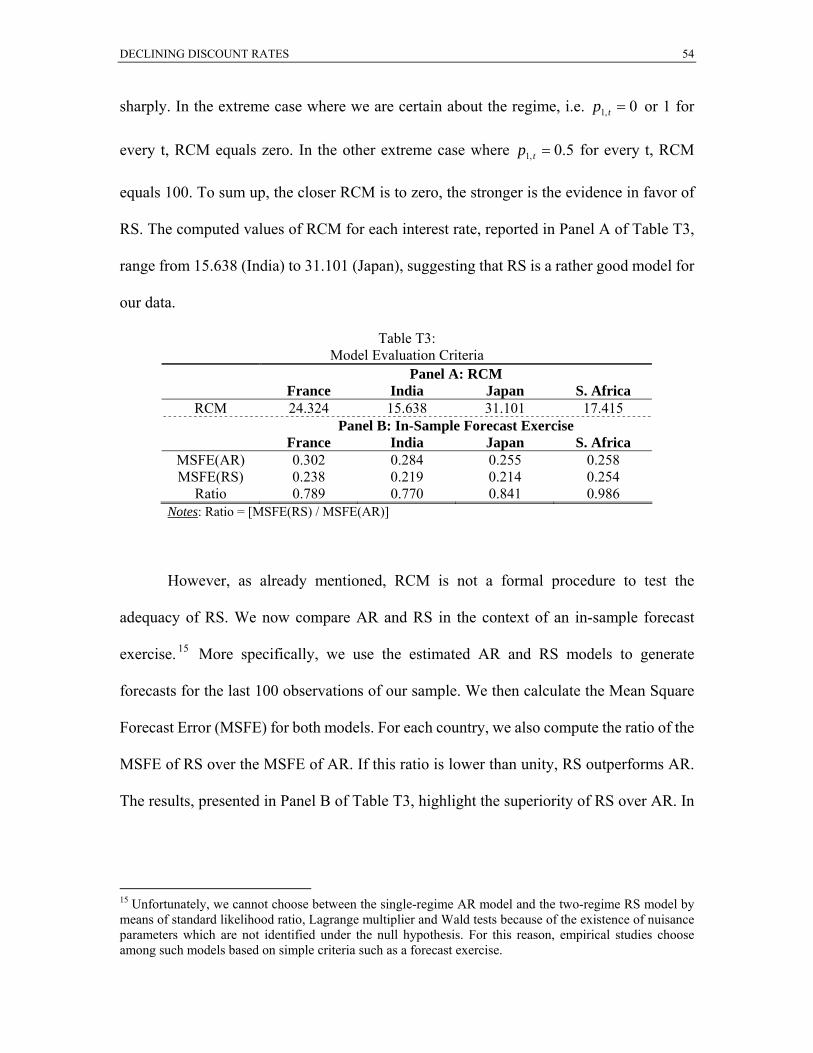
DECLINING DISCOUNT RATES 54
sharply. In the extreme case where we are certain about the regime, i.e. or 1 for
every t, RCM equals zero. In the other extreme case where
0,1 =tp
5.0,1 =tp for every t, RCM
equals 100. To sum up, the closer RCM is to zero, the stronger is the evidence in favor of
RS. The computed values of RCM for each interest rate, reported in Panel A of Table T3,
range from 15.638 (India) to 31.101 (Japan), suggesting that RS is a rather good model for
our data.
Table T3: Model Evaluation Criteria
Panel A: RCM France India Japan S. Africa
RCM 24.324 15.638 31.101 17.415 Panel B: In-Sample Forecast Exercise France India Japan S. Africa
MSFE(AR) 0.302 0.284 0.255 0.258 MSFE(RS) 0.238 0.219 0.214 0.254
Ratio 0.789 0.770 0.841 0.986 Notes: Ratio = [MSFE(RS) / MSFE(AR)]
However, as already mentioned, RCM is not a formal procedure to test the
adequacy of RS. We now compare AR and RS in the context of an in-sample forecast
exercise. 15 More specifically, we use the estimated AR and RS models to generate
forecasts for the last 100 observations of our sample. We then calculate the Mean Square
Forecast Error (MSFE) for both models. For each country, we also compute the ratio of the
MSFE of RS over the MSFE of AR. If this ratio is lower than unity, RS outperforms AR.
The results, presented in Panel B of Table T3, highlight the superiority of RS over AR. In
15 Unfortunately, we cannot choose between the single-regime AR model and the two-regime RS model by means of standard likelihood ratio, Lagrange multiplier and Wald tests because of the existence of nuisance parameters which are not identified under the null hypothesis. For this reason, empirical studies choose among such models based on simple criteria such as a forecast exercise.
DECLINING DISCOUNT RATES 55
general, the results show strong evidence in favor of RS. The only exception is South
Africa where the superiority of RS is marginal.
In summary, the picture emerging from (i) the rolling estimation of AR models, (ii)
RCM and (iii) the in-sample forecast exercise, support the utilization of RS to describe the
real interest rates under consideration.
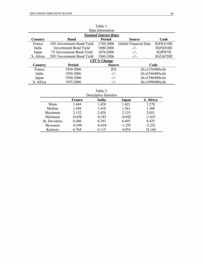
DECLINING DISCOUNT RATES 56
Table 1: Data Information
Nominal Interest Rates
Country Bond Period Source Code France 10Y Government Bond Yield 1746-2006 Global Financial Data IGFRA10D India Government Bond Yield 1800-2006 -//- IGIND10D Japan 7Y Government Bond Yield 1870-2006 -//- IGJPN7D
S. Africa 20Y Government Bond Yield 1860-2006 -//- IGZAF20D CPI % Change
Country Period Source Code France 1950-2006 IFS ifs:s1326400xzfa India 1950-2006 -//- ifs:s5346400xzfa Japan 1950-2006 -//- ifs:s1586400xzfa
S. Africa 1955-2006 -//- ifs:s1996400xzfa
Table 2: Descriptive Statistics
France India Japan S. Africa Mean 1.444 1.428 1.423 1.278
Median 1.456 1.410 1.561 1.368 Maximum 3.132 2.420 2.135 2.051 Minimum -0.698 -0.183 -0.042 -1.435
St. Deviation 0.486 0.393 0.495 0.435 Skewness -0.590 -0.434 -1.293 -3.232 Kurtosis 6.764 6.115 4.054 18.160
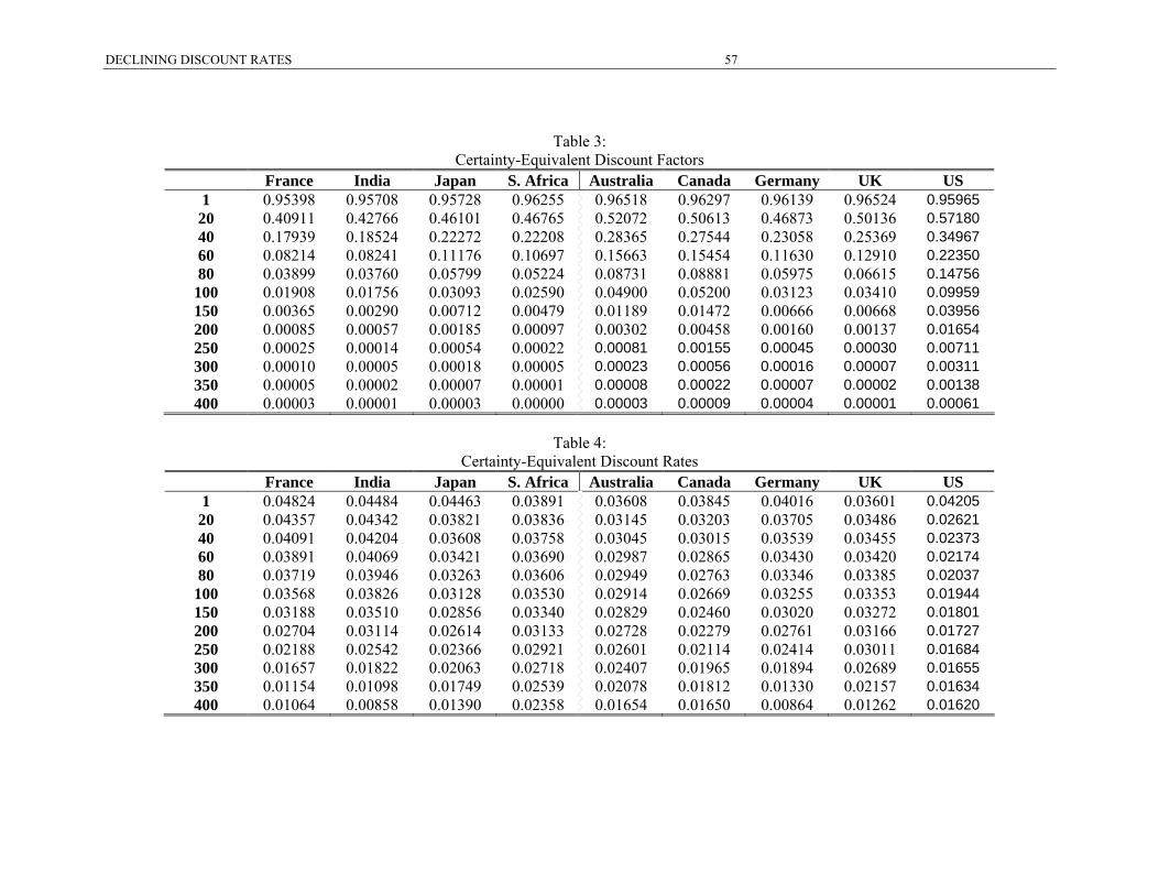
DECLINING DISCOUNT RATES 57
Table 3: Certainty-Equivalent Discount Factors
France India Japan S. Africa Australia Canada Germany UK US 1 0.95398 0.95708 0.95728 0.96255 0.96518 0.96297 0.96139 0.96524 0.95965
20 0.40911 0.42766 0.46101 0.46765 0.52072 0.50613 0.46873 0.50136 0.57180 40 0.17939 0.18524 0.22272 0.22208 0.28365 0.27544 0.23058 0.25369 0.34967 60 0.08214 0.08241 0.11176 0.10697 0.15663 0.15454 0.11630 0.12910 0.22350 80 0.03899 0.03760 0.05799 0.05224 0.08731 0.08881 0.05975 0.06615 0.14756
100 0.01908 0.01756 0.03093 0.02590 0.04900 0.05200 0.03123 0.03410 0.09959 150 0.00365 0.00290 0.00712 0.00479 0.01189 0.01472 0.00666 0.00668 0.03956 200 0.00085 0.00057 0.00185 0.00097 0.00302 0.00458 0.00160 0.00137 0.01654 250 0.00025 0.00014 0.00054 0.00022 0.00081 0.00155 0.00045 0.00030 0.00711 300 0.00010 0.00005 0.00018 0.00005 0.00023 0.00056 0.00016 0.00007 0.00311 350 0.00005 0.00002 0.00007 0.00001 0.00008 0.00022 0.00007 0.00002 0.00138 400 0.00003 0.00001 0.00003 0.00000 0.00003 0.00009 0.00004 0.00001 0.00061
Table 4: Certainty-Equivalent Discount Rates
France India Japan S. Africa Australia Canada Germany UK US 1 0.04824 0.04484 0.04463 0.03891 0.03608 0.03845 0.04016 0.03601 0.04205
20 0.04357 0.04342 0.03821 0.03836 0.03145 0.03203 0.03705 0.03486 0.02621 40 0.04091 0.04204 0.03608 0.03758 0.03045 0.03015 0.03539 0.03455 0.02373 60 0.03891 0.04069 0.03421 0.03690 0.02987 0.02865 0.03430 0.03420 0.02174 80 0.03719 0.03946 0.03263 0.03606 0.02949 0.02763 0.03346 0.03385 0.02037
100 0.03568 0.03826 0.03128 0.03530 0.02914 0.02669 0.03255 0.03353 0.01944 150 0.03188 0.03510 0.02856 0.03340 0.02829 0.02460 0.03020 0.03272 0.01801 200 0.02704 0.03114 0.02614 0.03133 0.02728 0.02279 0.02761 0.03166 0.01727 250 0.02188 0.02542 0.02366 0.02921 0.02601 0.02114 0.02414 0.03011 0.01684 300 0.01657 0.01822 0.02063 0.02718 0.02407 0.01965 0.01894 0.02689 0.01655 350 0.01154 0.01098 0.01749 0.02539 0.02078 0.01812 0.01330 0.02157 0.01634 400 0.01064 0.00858 0.01390 0.02358 0.01654 0.01650 0.00864 0.01262 0.01620
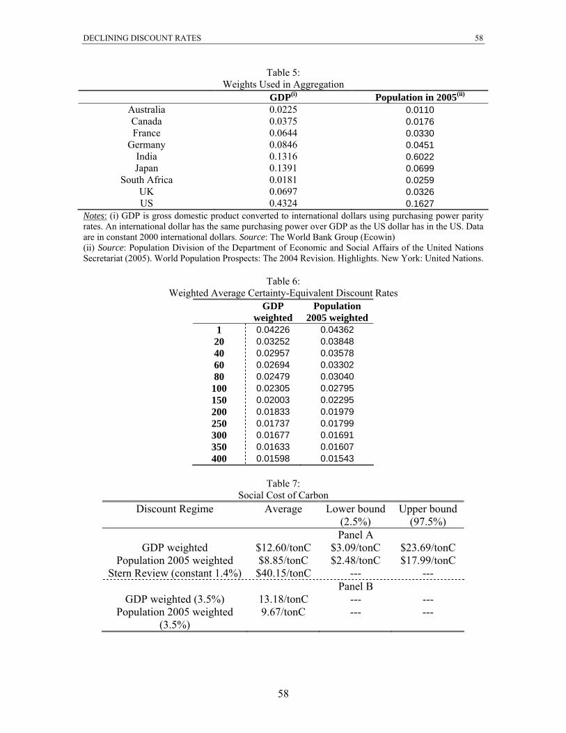
DECLINING DISCOUNT RATES 58
58
Table 5: Weights Used in Aggregation
GDP(i) Population in 2005(ii)
Australia 0.0225 0.0110 Canada 0.0375 0.0176 France 0.0644 0.0330
Germany 0.0846 0.0451 India 0.1316 0.6022 Japan 0.1391 0.0699
South Africa 0.0181 0.0259 UK 0.0697 0.0326 US 0.4324 0.1627
Notes: (i) GDP is gross domestic product converted to international dollars using purchasing power parity rates. An international dollar has the same purchasing power over GDP as the US dollar has in the US. Data are in constant 2000 international dollars. Source: The World Bank Group (Ecowin) (ii) Source: Population Division of the Department of Economic and Social Affairs of the United Nations Secretariat (2005). World Population Prospects: The 2004 Revision. Highlights. New York: United Nations.
Table 6: Weighted Average Certainty-Equivalent Discount Rates
GDP weighted
Population 2005 weighted
1 0.04226 0.04362 20 0.03252 0.03848 40 0.02957 0.03578 60 0.02694 0.03302 80 0.02479 0.03040
100 0.02305 0.02795 150 0.02003 0.02295 200 0.01833 0.01979 250 0.01737 0.01799 300 0.01677 0.01691 350 0.01633 0.01607 400 0.01598 0.01543
Table 7:
Social Cost of Carbon Discount Regime Average Lower bound
(2.5%) Upper bound
(97.5%) Panel A
GDP weighted $12.60/tonC $3.09/tonC $23.69/tonC Population 2005 weighted $8.85/tonC $2.48/tonC $17.99/tonC
Stern Review (constant 1.4%) $40.15/tonC --- --- Panel B
GDP weighted (3.5%) 13.18/tonC --- --- Population 2005 weighted
(3.5%) 9.67/tonC --- ---
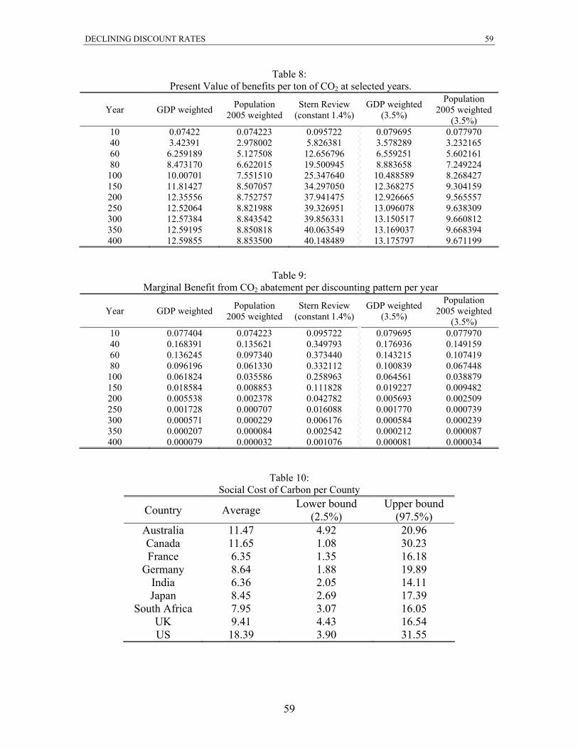
DECLINING DISCOUNT RATES 59
Table 8: Present Value of benefits per ton of CO2 at selected years.
Year GDP weighted Population 2005 weighted
Stern Review (constant 1.4%)
GDP weighted (3.5%)
Population 2005 weighted
(3.5%) 10 0.07422 0.074223 0.095722 0.079695 0.077970 40 3.42391 2.978002 5.826381 3.578289 3.232165 60 6.259189 5.127508 12.656796 6.559251 5.602161 80 8.473170 6.622015 19.500945 8.883658 7.249224 100 10.00701 7.551510 25.347640 10.488589 8.268427 150 11.81427 8.507057 34.297050 12.368275 9.304159 200 12.35556 8.752757 37.941475 12.926665 9.565557 250 12.52064 8.821988 39.326951 13.096078 9.638309 300 12.57384 8.843542 39.856331 13.150517 9.660812 350 12.59195 8.850818 40.063549 13.169037 9.668394 400 12.59855 8.853500 40.148489 13.175797 9.671199
Table 9: Marginal Benefit from CO2 abatement per discounting pattern per year
Year GDP weighted Population 2005 weighted
Stern Review (constant 1.4%)
GDP weighted (3.5%)
Population 2005 weighted
(3.5%) 10 0.077404 0.074223 0.095722 0.079695 0.077970 40 0.168391 0.135621 0.349793 0.176936 0.149159 60 0.136245 0.097340 0.373440 0.143215 0.107419 80 0.096196 0.061330 0.332112 0.100839 0.067448 100 0.061824 0.035586 0.258963 0.064561 0.038879 150 0.018584 0.008853 0.111828 0.019227 0.009482 200 0.005538 0.002378 0.042782 0.005693 0.002509 250 0.001728 0.000707 0.016088 0.001770 0.000739 300 0.000571 0.000229 0.006176 0.000584 0.000239 350 0.000207 0.000084 0.002542 0.000212 0.000087 400 0.000079 0.000032 0.001076 0.000081 0.000034
Table 10: Social Cost of Carbon per County
Country Average Lower bound (2.5%)
Upper bound (97.5%)
Australia 11.47 4.92 20.96 Canada 11.65 1.08 30.23 France 6.35 1.35 16.18
Germany 8.64 1.88 19.89 India 6.36 2.05 14.11 Japan 8.45 2.69 17.39
South Africa 7.95 3.07 16.05 UK 9.41 4.43 16.54 US 18.39 3.90 31.55
59
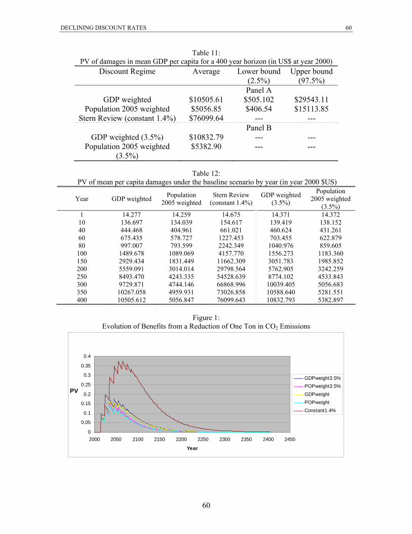
DECLINING DISCOUNT RATES 60
Table 11: PV of damages in mean GDP per capita for a 400 year horizon (in US$ at year 2000)
Discount Regime Average Lower bound (2.5%)
Upper bound (97.5%)
Panel A GDP weighted $10505.61 $505.102 $29543.11
Population 2005 weighted $5056.85 $406.54 $15113.85 Stern Review (constant 1.4%) $76099.64 --- ---
Panel B GDP weighted (3.5%) $10832.79 --- ---
Population 2005 weighted (3.5%)
$5382.90 --- ---
Table 12:
PV of mean per capita damages under the baseline scenario by year (in year 2000 $US)
Year GDP weighted Population 2005 weighted
Stern Review (constant 1.4%)
GDP weighted (3.5%)
Population 2005 weighted
(3.5%) 1 14.277 14.259 14.675 14.371 14.372
10 136.697 134.039 154.617 139.419 138.152 40 444.468 404.961 661.021 460.624 431.261 60 675.435 578.727 1227.453 703.455 622.879 80 997.007 793.599 2242.349 1040.976 859.605 100 1489.678 1089.069 4157.770 1556.273 1183.360 150 2929.434 1831.449 11662.309 3051.783 1985.852 200 5559.091 3014.014 29798.564 5762.905 3242.259 250 8493.470 4243.335 54528.639 8774.102 4533.843 300 9729.871 4744.146 66868.996 10039.405 5056.683 350 10267.058 4959.931 73026.858 10588.640 5281.551 400 10505.612 5056.847 76099.643 10832.793 5382.897
Figure 1:
Evolution of Benefits from a Reduction of One Ton in CO2 Emissions
PV
0
0.05
0.1
0.15
0.2
0.25
0.3
0.35
0.4
2000 2050 2100 2150 2200 2250 2300 2350 2400 2450
Year
GDPweight3.5%POPweight3.5%GDPweightPOPweightConstant1.4%
60
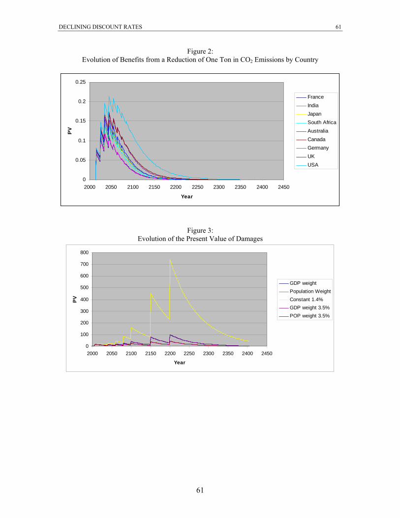
DECLINING DISCOUNT RATES 61
61
Figure 2: Evolution of Benefits from a Reduction of One Ton in CO2 Emissions by Country
0
0.05
0.1
0.15
0.2
0.25
2000 2050 2100 2150 2200 2250 2300 2350 2400 2450
Year
PV
FranceIndiaJapanSouth AfricaAustraliaCanadaGermanyUKUSA
Figure 3: Evolution of the Present Value of Damages
0
100
200
300
400
500
600
700
800
2000 2050 2100 2150 2200 2250 2300 2350 2400 2450
Year
PV
GDP weightPopulation WeightConstant 1.4%GDP weight 3.5%POP weight 3.5%
Top Related