THEORETICAL JUSTIFICATIONS FOR RATE DECLINE TRENDS IN ...

THEORETICAL JUSTIFICATIONS FOR RATE

DECLINE TRENDS IN SOLUTION-GAS DRIVE

RESERVOIRS, AND RESERVOIR PROPERTY

ESTIMATION USING PRODUCTION DATA

A THESIS SUBMITTED TO THE DEPARTMENT OF

PETROLEUM ENGINEERING

OF AFRICAN UNIVERSITY OF SCIENCE AND TECHNOLOGY, ABUJA

IN PARTIAL FULFILMENT OF THE REQUIREMENTS FOR THE DEGREE OF

MASTER OF SCIENCE IN PETROLEUM ENGINEERING

By

MOSOBALAJE Olatunde Olu

DECEMBER 2011

ii

THEORETICAL JUSTIFICATIONS FOR RATE DECLINE TRENDS

IN SOLUTION-GAS DRIVE RESERVOIRS, AND RESERVOIR

PROPERTY ESTIMATION USING PRODUCTION DATA

By

MOSOBALAJE Olatunde Olu

RECOMMENDED:

___________________________________

Chair, Professor Djebbar Tiab

___________________________________

Professor Samuel Osisanya

___________________________________

Dr. Alpheus Igbokoyi

APPROVED:

___________________________________

Chief Academic Officer

iii

to the ONLY WISE GOD …

iv

TABLE OF CONTENTS

List of Figures vii

List of Tables viii

Acknowledgements ix

Abstract x

1. Introduction 1

1.1 Overview of Rate Decline Analysis …………………………………………….. 1

1.2 Statement of Problem ………………………………………………………………. 3

2 Literature Review 5

2.1 Fundamentals of Empirical Decline Curves Analysis ………………… 5

2.2 Modern Decline Curve Analysis ………………………………………………. 6

2.3 Effects of Reservoir/Fluid Properties and Drive Mechanism on

Production Rate Decline …………………………………………………………. 8

2.4 Performance Prediction of Two-Phase Flows in Saturated

Reservoirs ……………………………………………………………………………… 11

2.4.1 Material Balance for Saturated Reservoirs ……………………… 12

2.4.2 Inflow Performance Relationships for Solution-Gas Drive

Reservoirs …………………………………………………………………….. 13

2.4.3 Diffusivity Equation for Solution-Gas Drive Reservoirs ….. 17

2.5 Decline Curves Analysis for Multi-Phase Flows ……………………… 20

2.6 Theoretical Basis for Decline Curves Analysis in Solution-Gas

Drive Reservoirs …………………………………………………………………… 22

2.6.1 Fetkovich Type Curves …………………………………………………. 22

2.6.2 Camacho and Raghavan Attempt ………………………………….. 25

2.6.3 The Non-Darcy Considerations ……………………………………. 27

3. Theoretical Developments 29

3.1 Overview and Background Information ………………………....... 29

v

3.2 Relationship between Empirical and Theoretical Decline

Parameters ………………………………………………………………………. 30

3.2.1 Derivation of Relationship ……………………………………….. 32

3.2.2 Significance of Relationship: Permeability Estimation ... 35

3.3 Considerations for the Effects of Non-Darcy Flow on the

Decline Parameter …………………………………………………………... 36

3.4 Inner Boundary Condition and the Existence of Hyperbolic

Family in Solution-Gas Drive Reservoirs ……………………………. 46

4. Simulation and Computational Procedures 52

4.1 Reservoir and Fluid Data Set ……………………………........................ 53

4.2 Simulation Data Deck and Run Specifications……………………. 58

4.2.1 Simulation Data Deck ……………………………………………… 58

4.2.2 Simulation Specifications and Controls …………………… 59

4.2.3 Output Requests ……………………………………………………. 60

4.2.4 Simulation Initial Solution ……………………………………… 62

4.3 Computational Procedures ……………………………………………. 62

5. Verification of Theories and Reservoir Property Estimation 66

5.1 Theoretical Decline Parameter Trend through Time …… 67

5.2 Theoretical Justifications for the Decline Parameters Trend …. 68

5.3 Effects of Incorporating Non-Darcy Flow …………………………… 71

5.4 Verification of Derived Relationships ………………………………….. 73

5.5 Proposed Reservoir Property Estimation Techniques ………… 76

5.5.1 Reservoir Permeability Estimation: Procedures and

Application ………………………………………………………………… 76

5.5.2 Reservoir Radius Estimation ……………………………………… 82

5.6 Sensitivity Analysis …………………………………………………………….. 83

5.6.1Case 1: Effects of Critical Gas Saturation …………………….. 84

5.6.2 Case 2: Effects of Permeability Value …………………………. 87

5.6.3 Case 3: Effects of Reservoir Drainage Radius …………….. 89

5.6.4 Case 4: Effects of Critical Bottomhole Pressure…………… 92

5.6.5 Case 5: Effects of Peak/Initial Rate ……………………………. 95

vi

5.6.6 Case 6: Effects of Reservoir Heterogeneity ………………. 99

6. Conclusions and Recommendations 103

Nomenclature 108

References 109

Appendix 113

vii

LIST OF FIGURES

1.1 Typical Oil Well Production Profile ………………………………………………………… 1

4.1 Oil PVT Properties ………………………………………………………………………………….. 55

4.2 Gas PVT Properties ………………………………………………………………………………… 56

4.3 Relative Permeability Characteristic Curves …………………………………………….. 58

5.1 Base Case: Production History: Rate-Time and Solution-Gas Drive Index …. 67

5.2 Base Case: Theoretical �� Trend through Time ………………………………………… 68

5.3: Base Case: Theoretical �� and �� through Time ………………………………… 72

5.4: Base Case: Verification of Equations 3.8 and 3.9 ……………………………………… 75

5.5: Base Case: Permeability Estimates through Time …………………………………….. 80

5.6: Comparing Permeability Estimates using different Techniques ………………… 81

5.7: Base Case: Reservoir Radius (re) Estimates through Time ………………………… 83

5.8: Case 1: Production History: Rate-Time and Solution-gas Drive Index ………… 84

5.9: Producing Gas-Oil Ratio, GOR Trend: Base Case and Case 1 ………………………. 85

5.10: Case 1: Theoretical �� Trend through Time …………………………………………….. 86

5.11: Case 1: Permeability Estimates through Time ………………………………………….. 87

5.12: Case 2: Theoretical �� Trend through Time…………………………………………….. 88

5.13: Case 2: Permeability Estimates through Time ………………………………………… 89

5.14: Case 3: Theoretical �� Trend through Time …………………………………………… 90

5.15: Case 3: Reservoir Radius (re) Estimates through Time ……………………………. 92


5.17: Case 4: Permeability Estimates through Time …………………………………………. 94

5.18: Case 4: Verification of Equations 3.8 and 3.9 …………………………………………. 95

5.19: Case 5: Production History: Rate-Time and Solution Gas Drive Index……… 96


5.21: Case 5: Permeability Estimates through Time ……………………………………….. 98

5.22: Case 5: Reservoir Radius (re) Estimates through Time ………………………….. 98

5.23: Case 6a: Verification of Equations 3.8 and 3.9 ………………………………………. 100

5.25: Case 6a: Permeability Estimates through Time ……………………………………. 101

5.26: Case 6b: Permeability Estimates through Time …………………………………… 102

viii

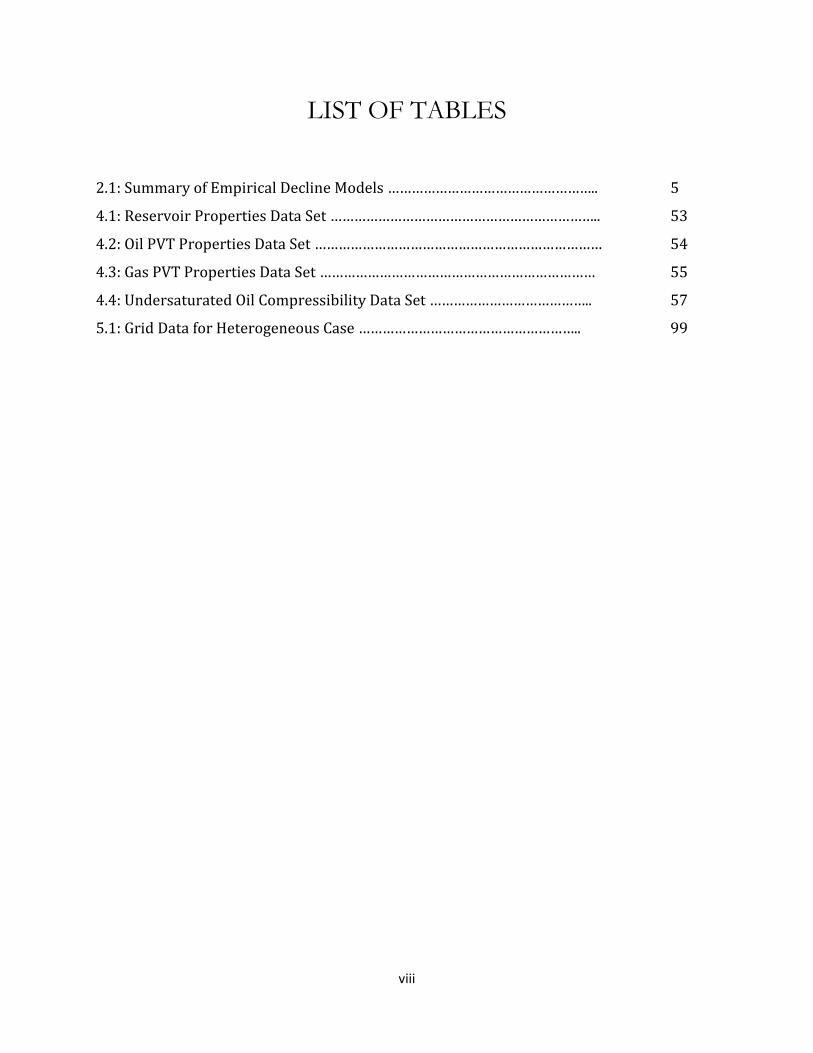
LIST OF TABLES

2.1: Summary of Empirical Decline Models …………………………………………….. 5

4.1: Reservoir Properties Data Set ………………………………………………………….. 53

4.2: Oil PVT Properties Data Set ……………………………………………………………… 54

4.3: Gas PVT Properties Data Set …………………………………………………………… 55

4.4: Undersaturated Oil Compressibility Data Set ………………………………….. 57

5.1: Grid Data for Heterogeneous Case ……………………………………………….. 99

ix

AKNOWLEDGEMENTS

I would like to thank my Supervisor, Professor Djebbar Tiab, first for his enthusiasm about

the proposal for this work, and then for his patience and guidance through the course of

this work. Dr. Alpheus Igbokoyi’s timely reviews are equally appreciated.

Valuable discussions I had with my colleagues, Anthony Ike, Oscar Ogali and Salako Rashidi

were crucial to the successful and timely completion of this work.

At different times I had to consult the following for expert’s advice: Dr. Nnaemeka Ezekwe

(BP), Professor Emeritus D.O Ogbe (Greatland Solutions) and Mr. Kingsley Akpara

(Schlumberger); many thanks to you, sirs.

Computational facility was provided by Schlumberger through a donation to African

University of Science and Technology, AUST, Abuja

I wish to thank Micah Maku for lending me his PC for this work.

Finally, to all those who wished and prayed for the success of this endeavor, I cannot say

enough of you all – million thanks!

x

ABSTRACT

Rate decline analysis is an essential tool in predicting reservoir performance and formation

property estimation. The use of historical production data to predict future performance is

the focus of the empirical domain of decline analysis while the theoretical domain focuses

on the use of such data to estimate formation properties.

A number of attempts have been made to establish the theories of rate decline in solution-

gas drive reservoirs. Such attempts have established the theoretical decline exponent b as a

function of formation properties. However, none of the attempts have established a direct

link between the empirical and theoretical domains of decline analysis. The purpose of this

work is to establish the missing link and deploy such link in reservoir property estimation.

In this work, a functional relationship (equation) between the empirical (��) and the

theoretical (��) was derived; based on the definition of a new parameter known as time-

weighted average of the theoretical exponent, ��. This new parameter was found to be

related to the empirical exponent, �� thus establishing the link. Theoretical justifications

for the ranges of values of the theoretical exponent were also offered. Consequent upon the

establishment of the relationship, this work developed a new improved technique for

estimating reservoir permeability. The technique was applied to a number of cases and was

found to yield excellent estimates of permeability even for an heterogeneous reservoir.

Sensitivity analyses were performed on the results. The work also investigated non-Darcy

flow effects on decline parameters. Lastly, this work provided mathematical justification

for the existence of the hyperbolic family of curves in solution-gas drive reservoirs.

1

CHAPTER 1

INTRODUCTION

1.1 OVERVIEW OF RATE DECLINE ANALYSIS

Production rate decline analysis is an essential tool for predicting reservoir/well

performance and for estimating reservoir properties. The production life of hydrocarbon

reservoirs typically shows three phases: the build-up phase, the peak phase, and the rate

decline phase1. The build-up phase corresponds to the increasing field production rate as

new wells are drilled. Thereafter, the field peak rate is attained and maintained for some

time after which the rate decline phase sets in. For a well, during the peak phase, the

bottomhole flowing pressure �� declines until it reaches a critical value, �� whereupon

the production begins to decline as the critical bottomhole pressure �� is maintained3.

Figure 1.1: Typical Oil Well Production Profile

0

50

100

150

200

250

0 500 1000 1500 2000 2500 3000

Oil

Pro

du

ctio

n R

ate

, q

(ST

B/D

)

Time, t (Days)

Typical Oil Well Production Profile

Prediction: Future Performance

Rate declines; �� is maintained

Attainment of ��

Constant production rate; declining ��

2

If there is no external influence on the factors affecting production, the decline period

would follow a fairly regular trend; hence analysis of the historical data could be useful in

predicting the future performance of the field3,4. However, decline curve analysis is to a

large extent based on Arps2 empirical models that have only little theoretical basis. The use

of historical production data to predict future performance is the focus of the empirical

domain of decline analysis while the theoretical domain focuses on the use of such data to

estimate formation properties.

The empirical analysis typically involves plotting the historical data against time and

extrapolating the curve to the future to predict the future performance. This extrapolation

is strictly based on the assumption that the controlling factors of the past production trend

will continue into the future and that the well must have been producing at full capacity4. In

a rather more rigorous approach, decline curve analysis involves the mathematical

estimation of the decline model parameters and then the substitutions of such estimated

parameters into the model equations to estimate recoverable reserves and predict future

production rates.4 The estimation of recoverable reserves leads to the economic evaluation

of oil properties (assets) while the prediction of future performance gives a measure of the

revenue generation pattern of oil field development projects. Both oil property evaluation

and revenue generation pattern prediction are essential in carrying out capital investment

analysis before scarce resources are committed5.

The theoretical approach of decline analysis is primarily concerned with investigating the

various reservoir/fluid factors that governs the past production trend and the effects of

these factors on the empirical decline model parameters. These factors include relative

3

permeability characteristics of the rock, fluid PVT properties, rock properties, wellbore

conditions and the prevailing drive mechanism in the reservoir.6-11 The essence of the

theoretical approach is to derive functional relationships between the empirical decline

model parameters and the physical reservoir/fluid properties. Such relationships are

useful in formulating procedures for reservoir properties estimation using field production

data in a kind of inverse problem. The compelling advantage of this approach to formation

evaluation lies in the fact that the data required are easy (inexpensive, requires no shut-in)

to acquire and to analyze.

1.2 STATEMENT OF PROBLEM

Many previous attempts12-15 at establishing functional relationships between the empirical

decline model parameters and the physical reservoir/fluid properties have been concerned

primarily with the exponential decline of single phase oil reservoirs. A number of

attempts10 at establishing the theories of hyperbolic decline of solution-gas drive

reservoirs have yielded expressions relating the decline exponent � to reservoir/fluid

properties. However, the values computed from such expression, although theoretically

sound, are not constant through time. More disturbing is the fact that the values did not

exhibit any equivalence with the empirically determined decline exponent. This fact

suggests there is a missing link between the theoretical and the empirical domains of the

decline curves analysis.

The purpose of this work is therefore to establish the missing link, to derive a functional

relationship between the empirical decline exponent, ��and the theoretical decline

4

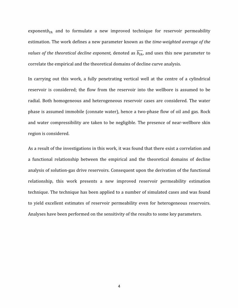
exponent�� and to formulate a new improved technique for reservoir permeability

estimation. The work defines a new parameter known as the time-weighted average of the

values of the theoretical decline exponent, denoted as ��, and uses this new parameter to

correlate the empirical and the theoretical domains of decline curve analysis.

In carrying out this work, a fully penetrating vertical well at the centre of a cylindrical

reservoir is considered; the flow from the reservoir into the wellbore is assumed to be

radial. Both homogeneous and heterogeneous reservoir cases are considered. The water

phase is assumed immobile (connate water), hence a two-phase flow of oil and gas. Rock

and water compressibility are taken to be negligible. The presence of near-wellbore skin

region is considered.

As a result of the investigations in this work, it was found that there exist a correlation and

a functional relationship between the empirical and the theoretical domains of decline

analysis of solution-gas drive reservoirs. Consequent upon the derivation of the functional

relationship, this work presents a new improved reservoir permeability estimation

technique. The technique has been applied to a number of simulated cases and was found

to yield excellent estimates of reservoir permeability even for heterogeneous reservoirs.

Analyses have been performed on the sensitivity of the results to some key parameters.

5

CHAPTER 2

LITERATURE REVIEW

2.1 FUNDAMENTALS OF EMPIRICAL DECLINE CURVES ANALYSIS

In 1944, Arps2 published a comprehensive review of methods of graphical analysis of

production decline behavior. Employing the concept of loss-ratio,16 he defined the relative

decline rate, D and the general decline equation known as Arps’ equation as follows:

1� �� 2.1�

Decline curve analysis is essentially based on three empirical mathematical models:

exponential decline, hyperbolic decline and harmonic decline.3 A summary of the governing

equations for each model is given in the table below.

Table 2.1: Summary of Empirical Decline Models

Model Relative Decline

Rate Equation

Rate-Time

Equation

Cumulative Production

Equation

Exponential �� 0�

1� �� ! � 1� ��

Hyperbolic �0 " � " 1�

1� �� 1 # ��$� ! � ��1 � �� %1 � & ��'$��(

Harmonic �� 1� 1� �� 1 # �� ! � �� )* &�� '

6

Nind17 provided plotting functions for the graphical analysis of rate data. Arps18 presented

methods for extrapolation of rate-time data to estimate primary oil reserves.

2.2 MODERN DECLINE CURVES ANALYSIS: TYPE CURVES

Conventional decline curve analysis involves the curve-fitting of past production data using

standard models4. The modern approach to decline analysis is the use of type curves to

analyze production data. A type curve is a plot of theoretical solutions to flow equations4.

The type curve decline analysis involves finding the type curve (theoretical solution) that

matches the actual production from a reservoir. The strengths of type curve decline

analysis over the conventional decline analysis are highlighted as follows:

• The type curve provides unique solutions; a task which is rather difficult with

conventional methods as results are subject to a wide range alternate

interpretaions12

• The type curves combine solutions to the flow equations both in the transient and

the pseudo-steady state regimes; this improves the uniqueness of the solution24.

• Reservoir properties such as permeability, skin and drainage radius can be

determined from type curve decline analysis6.

The deployment of type curves in analyzing production data was introduced by Slider19

and Gentry.20 Gentry manipulated the Arps’ relationships to solve for some group of

parameters in terms of other groups. With his solutions, Gentry constructed two graphs; on

each graph, a curve corresponds to each value of Arps’ exponent , �0 , � , 1�. The graphs

can be used to analyze actual production history.

7

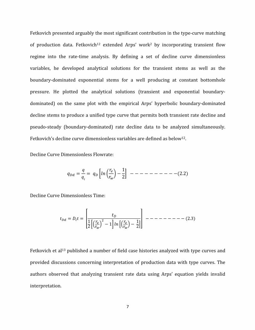
Fetkovich presented arguably the most significant contribution in the type-curve matching

of production data. Fetkovich12 extended Arps’ work2 by incorporating transient flow

regime into the rate-time analysis. By defining a set of decline curve dimensionless

variables, he developed analytical solutions for the transient stems as well as the

boundary-dominated exponential stems for a well producing at constant bottomhole

pressure. He plotted the analytical solutions (transient and exponential boundary-

dominated) on the same plot with the empirical Arps’ hyperbolic boundary-dominated

decline stems to produce a unified type curve that permits both transient rate decline and

pseudo-steady (boundary-dominated) rate decline data to be analyzed simultaneously.

Fetkovich’s decline curve dimensionless variables are defined as below12.

Decline Curve Dimensionless Flowrate:

��- � ��. � �� /)* &0�0�' � 121 � � � � � � � � � ��2.2�

Decline Curve Dimensionless Time:

��- � �� 2 ��12 /30�0�45 � 11 )* 630�0�4 � 1278 � � � � � � � � � �2.3�

Fetkovich et al13 published a number of field case histories analyzed with type curves and

provided discussions concerning interpretation of production data with type curves. The

authors observed that analyzing transient rate data using Arps’ equation yields invalid

interpretation.

8

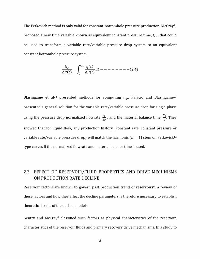
The Fetkovich method is only valid for constant-bottomhole pressure production. McCray21

proposed a new time variable known as equivalent constant pressure time, ��, that could

be used to transform a variable rate/variable pressure drop system to an equivalent

constant bottomhole pressure system.

!∆�� ; ��∆�� 2.4��=>?

Blasingame et al22 presented methods for computing ��. Palacio and Blasingame23

presented a general solution for the variable rate/variable pressure drop for single phase

using the pressure drop normalized flowrate, @∆A , and the material balance time,

B>@ . They

showed that for liquid flow, any production history (constant rate, constant pressure or

variable rate/variable pressure drop) will match the harmonic (� � 1) stem on Fetkovick12

type curves if the normalized flowrate and material balance time is used.

2.3 EFFECT OF RESERVOIR/FLUID PROPERTIES AND DRIVE MECHNISMS

ON PRODUCTION RATE DECLINE

Reservoir factors are known to govern past production trend of reservoirs6; a review of

these factors and how they affect the decline parameters is therefore necessary to establish

theoretical basis of the decline models.

Gentry and McCray6 classified such factors as physical characteristics of the reservoir,

characteristics of the reservoir fluids and primary recovery drive mechanisms. In a study to

9

investigate the effect of reservoir fluid and rock characteristics on production histories of

solution-gas drive reservoirs, Muskat and Taylor7 made the following conclusions:

1. The ultimate recovery of a solution-gas drive reservoir is very sensitive to oil

viscosity. The stock tank oil recovery decreases with increasing oil viscosity.

2. Increased solution gas oil ratio, CD would ordinarily favor increased recovery;

however, the consequent oil shrinkage results to lower recovery.

3. Additional gas provided by an overlying gas cap is less effective in oil expulsion than

the liberated solution gas.

4. Relative permeability characteristics that provide for no critical gas saturation

would lead to rapid increase in producing GOR.

5. The ultimate recovery is more sensitive to the relative permeability characteristics

at high liquid saturations than at lower liquid saturations

6. The ultimate reservoir volume voidage is less sensitive variations in rock and fluid

properties than is the ultimate stock tank recovery.

7. Due to the twin effects of reduced permeability to oil and increased oil viscosity as it

loses gas, the productivity indexes of well producing from a solution-gas drive will

continuously decrease.

Arps and Roberts8 found out that ultimate recovery increases with oil gravity except for

higher solution-gas oil ratios. They also reported that the rock type as identified by its

relative permeability characteristics have significant effect on recovery; with sandstones

reservoirs showing higher recovery than carbonate reservoirs.

10

Attempts have been made by various investigators to associate the decline model

parameters with the physical properties of the reservoir as well as the active drive

mechanism. Mead9 noted in his discussion of b factor (decline curve exponent) that: “as b

approaches zero, for the same initial maximum (peak) production rate and same ultimate

recovery, a greater and greater amount of oil can be produced before decline sets in.” This

means that as b approaches zero, the peak production phase of the reservoir is extended

and hence the decline phase is delayed. On the other hand, as b approaches zero, when the

decline finally sets in, it occurs rapidly.

Gentry and McCray6 conducted simulation studies in order to investigate the effect or

reservoir and fluid properties on the decline trend of solution-gas drive reservoirs. They

summarized their observations as follows:

1. The fluid properties and the reservoir dimensions had greater influence on the

decline parameter �� than did the relative permeability relationship. Specifically,

changing the fluid system resulted to 200% - 400% change in �� as compared to

15% - 18% change when relative permeability characteristics were altered.

2. Conversely, the relative permeability characteristics had greater influence on the

decline model parameter b than did the fluid properties. Changing relative

permeability characteristics resulted into b value changing from 0 to 1 on one

instance and from 0.3 to values above 1 on the other instance. Changing fluid system

however resulted in to b ranging from 0 to 0.3 on one instance and from 1.0 to

slightly above 1 on the other hand.

11

3. The parameter ��, a measure of the onset of decline phase depends on reservoir

properties such as absolute permeability and water saturation as well as the fluid

properties.

4. Separate zones producing into the same wellbore could have significant effects on

the decline parameters and could in fact produced values of b greater than 1.

In 1956, Mathews & Lefkovits11, conducted an experimental study with models and

theoretical deductions and they published results showing, that for a well with free surface

(secondary gas cap) in a homogeneous gravity drainage reservoir (dipping bed), the

decline is of the hyperbolic type with the hyperbolic exponent b having a value of 0.5 (b =

0.5). In 1958, Lefkovits and Matthews25 extended the experimental work to actual field

cases with results showing that when the well is producing from the two layers of different

thickness and permeability or two layers having different skin effects, the value of b may be

greater than 1; however, they predicted that the value of b would approach 0.5 again as the

higher permeability zone depletes.

2.4 PERFORMANCE PREDICTION OF TWO-PHASE FLOWS IN SATURATED

RESERVOIRS

Prediction of reservoir future performance (production rate as a function of time) typically

involves combining the reservoir material balance equations (!EF �� with well inflow

equations�� EF �� . The two performance data (!EF �; � EF �� are then correlated

with time to yield the rate-time performance4. Analytical solutions to diffusivity equation

also give rate-time performance.

12

2.4.1 Material Balance for Saturated Reservoirs

First, the material balance equation for a single-phase volumetric reservoir is commonly

presented thus4:

! � !H� & IJIJ�' ∆� � � � � � � � ��2.5�

The effective compressibility term, H� is defined by Hawkins26 as follows:

H� � LJ�HJ # L��H� # H 1 � L�� 2.6�

The material balance equation for a saturated volumetric reservoir is presented thus4:

! � !IJ # NO � !CDPIQ�IJ � IJ�� # �CD� � CD�IQ � � � � � � � ��2.7�

Equation 2.7 above contains two unknowns, ! �*� O . Many techniques employed in

performance prediction of saturated reservoirs are based on combining the MBE above

with the instantaneous GOR equation and the saturation equation4. One of such method is

the Muskat method. Muskat27 expressed the MBE for saturated volumetric reservoir as

follows:

�LSJ�� LSJIQIJ �CD�� # LSJIJ TUQTUJ VJVQ �IJ�� 1 � LSJ � L��IQ �IQ��1 # VJVQ TUQTUJ � � � � � � � � � �2.8�

13

In compact notation, equation the Muskat MBE is written thus:

�LJ�� LSJIJ�IJ�� # HS� XSJXS� � � � � � � � � � ��2.9�

In the above equation,

HS� � LSJIJ�IJ�� LSQIQ

�IQ�� # LSJIQIJ�CD�� 2.10�

XS� � XSJ # XSQ � TUJVJ # TUQVQ � � � � � � � ��2.11�

Camacho and Raghavan10 developed the MBE for saturated reservoir as follows:

�!�� HS�Z[\]5.614XS� � � � � � � � �2.15� Other forms of material balance equation for saturated reservoirs are the Tarner28 MBE

and the Tracy MBE29

2.4.2 Inflow Performance Relationships for Solution-gas Drive Reservoirs

The various material balance techniques described above show the relationship that exist

between the cumulative production, ! and the average reservoir pressure, �; however,

they do not relate the production rate to time. The correlation of production to time is

typically accomplished by the use of relationships that are designed to predict the flowrate

of wells. The functional representation of the relationship that exists between oil flowrate,

� and bottomhole flowing pressure, �� is called the inflow performance relationship, IPR4.

14

For a well producing from an undersaturated reservoir, the IPR is expressed thus4:

� � ^N� � �� P � � � � � � � � � �2.16�

The parameter ^ in the above equation is known as productivity index and given as follows:

^ � 0.00708T\VI 6)* 30�0�4 � 0.75 # F7 � � � � � � � �2.17�

Unlike the undersaturated reservoir, the productivity index of a well producing from a

solution-gas drive will continuously decrease due to the twin effects of reduced

permeability to oil as gas evolves out of solution and the increased oil viscosity as it loses

gas. Evinger and Muskat30 observed that a straight line IPR (constant productivity index)

may not be expected when two-phases are flowing in the reservoir. The relative

permeability characteristics, the viscosities and formation volume factors in solution-gas

drive reservoirs vary as function of average reservoir pressure and saturation. To account

for variation of the productivity index, a number of empirical IPRs have been developed to

predict the pressure-production rate behavior during two-phase flow in solution-gas drive

reservoirs.

In a simulation study involving twenty-one wide-ranged reservoir/fluid data sets, Vogel31

developed a quadratic IPR in terms of dimensionless flowrate and dimensionless pressure

to describe the pressure-production behavior of saturated reservoirs as follows:

�J�J,�_` � 1 � 0.2 &�� ' � 0.8 &�� '5 � � � � � � � � � ��2.18�

15

Fetkovich32 suggested the applicability of isochronal testing to oil wells; the isochronal

testing is originally based on the Rawlins and Schellhardt33 gas well deliverability equation.

Using multi-rate test data from forty wells in six different fields, Fetkovich proved the

suitability of the approach to oil wells performance prediction. He developed his IPR thus:

�J � aN�5 � �� 5P� � � � � � � � � � �2.19�

In a form similar to Vogel’s IPR, the Fetkovich IPR is represented thus:

�J�J,�_` � b1 � &�� '5c� � � � � � � � ��2.20�

Jones, Blount and Glaze31 proposed an IPR thus:

� � �� J � a # ��J � � � � � � � � � �2.21�

The above IPR was based on the Forchheimer’s35 non-Darcy flow model that divides flow

into laminar (Darcy) and turbulence (non-Darcy) components. In the above equation, a is

the laminar flow coefficient while � is the turbulence coefficient. The coefficients a �*� �

are determined from multipoint tests, thereafter; the performance of the well can be

predicted using the equation below:

�J � �a # da5 # 4�N� � �� P2�

16

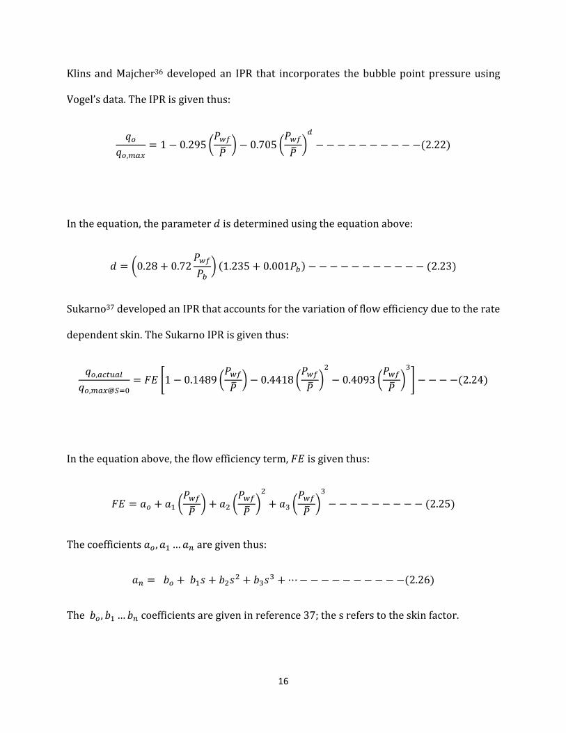
Klins and Majcher36 developed an IPR that incorporates the bubble point pressure using

Vogel’s data. The IPR is given thus:

�J�J,�_` � 1 � 0.295 &�� ' � 0.705 &�� '- � � � � � � � � � ��2.22�

In the equation, the parameter � is determined using the equation above:

� � &0.28 # 0.72 �� ' �1.235 # 0.001�� 2.23�

Sukarno37 developed an IPR that accounts for the variation of flow efficiency due to the rate

dependent skin. The Sukarno IPR is given thus:

�J,_��e_f�J,�_`@hi? � jk b1 � 0.1489 &�� ' � 0.4418 &�� '5 � 0.4093 &�� 'lc � � � ��2.24�

In the equation above, the flow efficiency term, jk is given thus:

jk � �J # �$ &�� ' # �5 &�� '5 # �l &�� 'l � � � � � � � � � �2.25�

The coefficients �J , �$ … �� are given thus:

�� J # �$F # �5F5 # �lFl # n � � � � � � � � � ��2.26�

The �J , �$ … �� coefficients are given in reference 37; the s refers to the skin factor.

17

Gallice and Wiggins38, in a comparative study of two-phase IPR correlations, gave

recommendations on the use of the IPR correlations described above, the collection of data

and the quality and reliability of the performance estimates made from such IPR

correlations. They concluded that the multipoint methods (Fetkovich and Jones, Blount and

Glaze gives better estimates than the single point methods (Vogel, Klins and Majacher, and

Sukarno).

Ilk et al39 provided the analytical developments of “Vogel” type IPR using characteristic

flow behavior.

2.4.3 Diffusivity Equation for Solution-gas Drive Reservoirs

The inflow performance relationship discussed above are based on statistical regression of

field data, hence the outcomes of using such correlations are dependent on the condition at

which the data are sampled40. Solution to diffusivity equation therefore provides analytical

approach to performance prediction is solution-gas drive reservoirs40.

The radial flow diffusivity equation for flow of any fluid in a porous media is given as41:

10 ��0 &ToV 0 �p�0' � [Ho q�q� � � � � � � � ��2.27�

This general equation above is non-linear as the coefficients of the equation are functions

of the dependent variable – pressure. With relevant assumptions pertinent to slightly

compressible liquid flow, equation 2.27 has been linearized and presented as follows41:

18

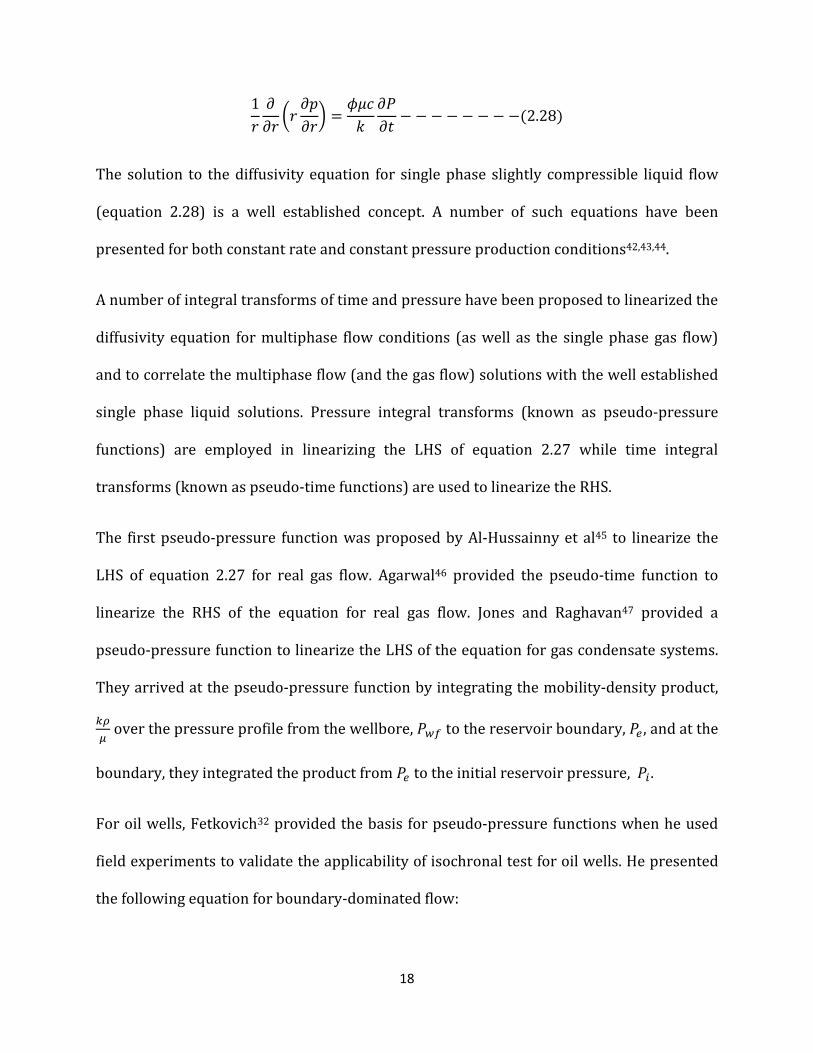
10 qq0 &0 qpq0' � [VHT q�q� � � � � � � � ��2.28�

The solution to the diffusivity equation for single phase slightly compressible liquid flow

(equation 2.28) is a well established concept. A number of such equations have been

presented for both constant rate and constant pressure production conditions42,43,44.

A number of integral transforms of time and pressure have been proposed to linearized the

diffusivity equation for multiphase flow conditions (as well as the single phase gas flow)

and to correlate the multiphase flow (and the gas flow) solutions with the well established

single phase liquid solutions. Pressure integral transforms (known as pseudo-pressure

functions) are employed in linearizing the LHS of equation 2.27 while time integral

transforms (known as pseudo-time functions) are used to linearize the RHS.

The first pseudo-pressure function was proposed by Al-Hussainny et al45 to linearize the

LHS of equation 2.27 for real gas flow. Agarwal46 provided the pseudo-time function to

linearize the RHS of the equation for real gas flow. Jones and Raghavan47 provided a

pseudo-pressure function to linearize the LHS of the equation for gas condensate systems.

They arrived at the pseudo-pressure function by integrating the mobility-density product,

rst over the pressure profile from the wellbore, �� to the reservoir boundary, �� , and at the

boundary, they integrated the product from �� to the initial reservoir pressure, �� .

For oil wells, Fetkovich32 provided the basis for pseudo-pressure functions when he used

field experiments to validate the applicability of isochronal test for oil wells. He presented

the following equation for boundary-dominated flow:

19

�J � T\141.2�ln 0�0� � 0.75 # F� ; & wUJVJI?' ��A��Ax � � � � � ��2.29�

Camacho and Raghavan48 provided solution-gas pseudo-pressure and pseudo-time

functions with which they were able to correlate solution-gas drive systems with single

phase slightly compressible liquid systems. Their pseudo-pressure and pseudo-time

functions and the consequent correlations of the solution-gas drive systems to single phase

systems was found to be valid for both transient and boundary-dominated flow and also

valid for constant-oil rate and constant-pressure production conditions. The Camacho and

Raghavan48 pseudo pressure definition is essentially a unification of similar definitions

given by references 32 and 49.

Their pseudo-pressure and pseudo-time definitions which were based on the Muskat’s

material balance equation27 are given as follows:

��0, �� ; & wUJVJI?' �� # ; % wUJVJI?( �� 2.30�A

A��A��

A�U,��

�̃z� � 0.006328T[]�� ; ��XS��HS{��? �� 2.31�

�|z� � 0.006328T[] ; XS��HS{��? �� 2.32�

Equation 2.32 is only valid for constant rate condition.

20

The Camacho and Raghavan work is valid for solution-gas drive reservoirs where oil is the

dominant flowing phase. Fraim and Wattenbarger50 extended the Camacho and Raghavan

work to predict the flow of all mobile phases. They achieved this by defining integral

transforms for time, pressure and rate known as equivalent liquid time, equivalent liquid

pressure and equivalent liquid rate respectively. The purpose of the Fraim and

Wattenbarger work was to develop a method to analyze multiphase flow with the

Fetkovich12 type curve (the exponential stem).

Marhaendrajana and Permadi40 presented pseudo-pressure and pseudo-time functions for

three phase flow that included oil water and gas.

2.5 DECLINE CURVES ANALYSIS FOR MULTIPHASE FLOWS

The Fetkovick12 unified type curve is made up of analytical stems (transients and

exponential boundary dominated) and empirical stems (boundary-dominated hyperbolic).

In order to perform a fully analytical decline analysis (for the purpose of parameter

estimation), multiphase flow systems are typically correlated with single phase slightly

compressible liquid system (exponential decline) to permit the use of Fetkovich’s type

curves as well as other existing type curves. The correlation is typically accomplished by

the use of special variables in place the conventional variables (time, flowrate).

One of such methods for analyzing production data of wells producing from a solution-gas

drive reservoir employs the use of special variables known as equivalent liquid time and

equivalent liquid rate; the method was proposed by Fraim and Wattenbarger50 This

method generates the equivalent total mass flow of multiple phases for the total history of

21

the well which can then be analyzed on any of the existing type curves. Frederick and

Kelkar51 modified the dimensionless rate and the dimensionless cumulative production

equations (defined by Fetkovich12 for single phase model) to generate a new set of

equations to approximate the ultimate recovery of solution-gas drive reservoirs.

Chen and Poston55 introduced the normalized pseudo-time to account for the effects of

variations in system mobility and compressibility. The rate-time data for the single phase

flow condition (exponential decline) characteristically yields a straight line on a semi-log

plot while the hyperbolic decline (multiphase) yields a non-linear relationship on the semi-

log plot4. The Chen and Poston normalized pseudo-time transform linearizes the semi-log

rate-time relationship for the multiphase case and thus removes the ambiguities inherent

in analyzing the hyperbolic decline trend. In essence, replacing the conventional ‘time’

variable with the ‘normalized pseudo-time’ on the semi-log analysis yields a straight line

for multiphase data. The pseudo-time and the pseudo-pressure terms in Chen and Poston

formulation are normalized by the initial conditions. A step-by-step procedure of this

technique is given in reference 55. The pseudo-time is defined thus55:

� � ; X H�}3X H�} 4�� 2.33��

�~

22

2.6 THEORETICAL BASIS FOR DECLINE CURVES ANALYSIS IN SOLUTION-

GAS DRIVE RESERVOIRS

A number of attempts have been made to analytically establish the theories of empirical

decline analysis and to express empirical decline parameters as functions of physical

reservoir and fluid properties. A result of such attempts is the establishment of the fact that

the exponential decline is a consequence of single phase slightly compressible liquid

production3,12 Guo et al3 showed that the relative decline rate and production rate decline

equations for exponential decline model can be derived rigorously by combining the

pseudo-steady state flow equation for a volumetric reservoir model with the single phase

material balance equation. They derived an analytical expression for the empirical decline

parameter, �� in terms of physical reservoir/fluid property thus:

�� T\141.2VH�!� 6)* 30.4720�0� 4 # F7 � � � � � � � �2.34�

2.6.1 Fetkovich Type Curves

Fetkovich,12 using a combination of simple material balance equation and the oil well rate-

pressure relationships previously developed in reference 32 was able to analytically derive

a rate-time relationship for single phase flow. The rate-time relationship so derived was a

form of the exponential decline equation but in terms of reservoir variables. From the

relationship, he developed an analytical expression for the empirical decline parameter, ��

in terms of physical reservoir/fluid property thus:

23

�� /0.00634T�VH�0�5 1 2 112 /30�0�45 � 11 6)* 30�0�4 � 1278 � � � � � � � � � ��2.35�

Additionally, Fetkovich12 combined analytical solution of the transient (early-time) period

with empirical solution of the boundary-dominated (late-time) period on the same log-log

dimensionless type curve. Hence, the type curves have two regions: the transient (early-

time) and the boundary-dominated (late-time) curves; this effectively encompasses the

entire production life. The entire Fetkovich type curve analysis is based on the following

dimensionless variables derived from the general Arps’ hyperbolic equation.

��- � �� 2.36�

��- � �� 2.37�

The early-time curves of Fetkovich type curves were gotten by transforming the analytical

constant well pressure solutions (for single phase slightly compressible liquid) of

diffusivity equation. The original solution has been presented in terms of dimensionless

flowrate and dimensionless43. The dimensionless flowrate and time are defined thus:

�.��*F.�*)�FF j)��0�� 141.3�VIT\�� 2.38�

�.��*F.*)�FF �.�� 0.00634T��VH�0�5 � � � � � � � �2.39�

24

Fetkovich transformed the solutions from the original variables �� and �� to the decline

dimensionless variables ��- and ��- using the following relationships which he had

derived12:

��- � �� /)* &0�0�' � 121 � �T\N�� P141.3�VI 6)* 30�0�4 � 127 � � � � � � � � � �2.40�

And

��- � 2 ��12 /30�0�45 � 11 )* 630�0�4 � 1278

� /0.00634T��VH�0�5 1 2 112 /30�0�45 � 11 )* 630�0�4 � 1278 � ��2.41�

The transformed solutions were plotted for various values ofU�Ux. At the onset of boundary-

dominated flow, all the curves were found to converge to a single exponential curve at ��

value of about 0.1. This shows that the late-time (boundary-dominated) behavior of the

system for all single phase reservoir sizes obeys the exponential decline model.

The late-time portion of the Fetkovich type curves were gotten by plotting the Arp’s

empirical equation in dimensionless terms given below as:

��- � 1�1 # ��-�$� � � � � � � � �2.42�

Plotting equation 2.42 above, i.e. ��- versus ��- for various values of b, it was found that all

the curves converged at �� = 0.3 to a single curve corresponding to b = 0.

25

2.6.2 Camacho and Raghavan Attempt

The theoretical considerations in the Fetkovich work were based on the assumption of a

single phase reservoir. For solution-gas drive reservoirs leading to hyperbolic decline,

Camacho and Raghavan10 provided a theoretically rigorous derivation of the decline

exponents�� *� ��. Using the pseudo-pressure and pseudo-time functions defined in

reference 48, they developed expressions for the dimensionless pseudo-pressure, ��

corresponding to the average reservoir pressures, in terms of the two dimensionless

pseudo-time definitions (equations 2.31 and 2.32 above). The expressions for the average

dimensionless pseudo-pressures are as follows:

�� T\141.2�� ; % wUJVJI?( �� A

A�� 2��̃z� � � � � � �2.43�

�� T\141.2�� ; % wUJVJI?( �� A

A�� 1 � exp %2��|z�� (� � � � � � �2.44�

Where � � $5 6)* �z��Ux� # 2F7

Differentiating equations 2.43 and 2.44 above and making a number of substitutions, the

authors obtained the following expression:

1� �� )*�� 2�0.006328T[]� X�H� � � � � � ��2.45�

26

Relating equation 2.45 above to Arps’ exponential rate-time equation (see table 2.1), they

showed that the empirical decline parameter �� can be expressed in terms of physical rock

and fluid properties thus:

�� 2�0.006328T & XSHS{'��] � � � � � � � �2.46�

Furthermore, employing the concept of loss ratio defined as follows: --� �1 -f�@-�� ,

they showed that the empirical decline parameter �� can be expressed in terms of physical

rock and fluid properties thus:

� � ��]2�0.006328T �� %HS{XS ( � � � � � � � �2.47�

The authors also gave a discussion on the conditions under which the Arps’ equation might

be used to analyze data thus:

1. If the ratio ��S� is approximately constant through time, then the rate data would fit to

the Arps’ exponential decline (� � 0�

2. If the ratio ��S� is a linear function of time, then the rate data would fit to a unique

member of the hyperbolic family (b = constant)

27

However, the authors observed from their simulation studies that the ratio ��S� varies non-

linearly with time. They also noted that the exponent � is not constant in most of the

theoretical studies.

2.6.3 The Non-Darcy Considerations

In the Camacho and Raghavan approach presented above, the non-Darcy flow caused by

near-wellbore turbulence effect was not considered. However, non-Darcy flow may be

considered as a normal occurrence in solution gas drive reservoirs52. In analyzing their

results, the authors10 noted that a given simulation rate data did not match a unique value

of exponent � on the Arps’ type curves; they suggested that in reality, the presence of rate-

dependent variable skin factor such as near wellbore non-Darcy flow effects could yield a

fairly constant value of exponent �. Non-Darcy effects are accounted for using one of the

equations below:

1. Forchheimer Equation53:

�p�0 � VT E # �oE5 � � � � � � � � � � � �2.48�

The parameter � in the expression above is known as the inertial coefficient and is

given as follows:

� � 48511��.�T?.� � � � � � � � � � ��2.49�

2. Rate-dependent variable skin factor54:

28

The total skin factor sT in the flow equation is seen as the sum of a constant

mechanical skin factor and a rate-dependent skin factor due to inertial/non-Darcy

flow effects.

F{ � F� # !� � � � � � � � � � �2.50�

Where ! is known as the Non-Darcy flow coefficient.

The non-Darcy flow coefficient and the inertial coefficient are also related as

follows54:

! � 1.027336 � 10�$��oT2�V\ & 10� � 10�' � � � � � � � � � ��2.51�

29

CHAPTER 3

THEORETICAL DEVELOPMENTS

3.1 OVERVIEW AND BACKGROUND INFORMATION

This work sets out essentially to investigate the fundamental theories of reservoir and fluid

interactions underlying the empirically established trends of rate decline in solution-gas

driver reservoirs. The motivation for the investigation was to establish a functional

relationship between the theoretical domain and the empirical domain; such a relationship

is useful not only in verifying results of empirical analyses but also in formulating

procedures for reservoir properties (permeability, drainage radius e.t.c.) estimation using

field production data.

The subject dealing with the empirical domain of rate decline trends in reservoir is known

as decline curve analysis (DCA) and is largely based on Arps2 1945 work. Typically, decline

curve analysis involves the determination of empirical parameters � �*� � in the Arps

30

equation; this is conventionally done by fitting historical rate-time data to the Arps general

equation. The parameter �, which assigns a given reservoir rate decline trend to a specific

member of the Arps hyperbolic family (0 , � , 1.0 ) is the focus of this work.

Essentially, the theories developed in this work are herein presented in three sections. The

foremost consideration in this work is the establishment of a functional relationship

between the empirical domain �� and the theoretical domain��. A consideration for

non-Darcy flow effects in the near wellbore region was then developed as an attempt to

investigate suggestions from various researchers10,32,52 on the effects of non-Darcy flow on

the � parameter. Lastly, a theoretical derivation is made to mathematically justify the

existence of the hyperbolic family of curves for solution-gas drive reservoirs. This

derivation is based on a novel concept of inner boundary condition of the diffusivity

equation in terms of solution-gas pseudo pressure and pseudo time functions.

3.2 RELATIONSHIP BETWEEN EMPIRICAL AND THEORETICAL DECLINE

PARAMETER (��EF ��)

The empirical domain of decline curves analysis is based on Arps2 general equation given

as follows:

� 1� �� > � � � � � � � ��3.1�

The parameter � has also been expressed in terms of physical reservoir and fluid

properties as follows10

31

�� []2�0.006328T � �� &HS�X�� ' � � � � � � � �3.2�

Note: In this work, the b parameter from the empirical domain has been denoted as ��

while that from the theoretical domain is denoted as ��; this is done to distinguish clearly

distinguish the two parameters for clarity sake.

Until now, it has been expected that the two parameters above (�� *� ��p ) represent

the same quantity; this expectation is expressed in suggestions by reference 10 on physical

phenomena that could yield a constant value of �� (through time) to match a given value of

��. However, simulations carried out in this work (and reported in chapter 5) yields

values of �� that varied considerably with time (for a given reservoir) and exhibited no

tendency for constancy even with considerations for non-Darcy flow near the wellbore as

suggested by reference 10.

Considering the above trend, this work then proposed the following hypothesis as being

the actual implications of �� values (through time) computed from reservoir and fluid

properties as compared to a given �� (constant value) computed empirically from

historical rate-time data.

a. The theoretical �� values could possibly not mean the same thing as the empirical

�� value

b. The theoretical values, �� could be seen as reflecting the actual dynamics of the

reservoir and the fluid behavior through time; hence it may be expected to have a

transient (varying) behavior against any anticipation for its constancy.

32

c. The empirical value �� might as well be seen as representing some sort of

weighted average of the theoretical values (��) over time.

d. If a relationship between �� and some sort of weighted average of �� values (say

�� ) could be derived, then such link will offer the opportunity for an improved

formation evaluation methods using decline curves analysis in solution-gas drive

reservoirs.

This work then defined a new parameter known as �� (being the time-weighted average of

�� values over time) and went further to derive a functional relationship between ��

and �� in the fourth point above. The derivation is presented below.

3.2.1 Derivation of Relationship

Since the �� values vary widely through time, it is convenient to say �� is a function of

time t and not a constant value through time (even with the so-called non-Darcy effect

considered)

� ��

A new parameter known as �� (being the time-weighted average of �� values over

time) is then defined in this work as follows:

�� ∑ �� .*H0��*��) �.�� )�pF��) �.�� )�pF�� F.*H� ��H).*� That is,

33

�� ∑ 3�� N�� $�P4� �� J � � � � � � � � � ��3.3�

The time denoted by �J in the equation above corresponds to the onset of decline.

The summation term above was then represented by an integral of �� , thus;

�� ∑ N�� $�P� �� J � � �� J � � �� J � � � ��3.4�

Since equation 3.2 above gives values of �� varying with time, the RHS of equation 3.2 can

be taken as �� .

Equation 3.2 was then substituted into equation 3.4 to yield the following:

�� []2�0.006328T � �� &HS{X{' �� J

� �� []�2�0.006328T &HS{X{'�� J � � � � � � � �3.5�

But reference 10 has shown that � 5 ?.??¡l5¢r£z� ��S� � -f�@-�

Then,

� []�2�0.006328T %HS{X{( � 1�)*�� 11� �� 3.6�

34

Substitution of equation 3.6 into equation 3.5 yielded the following:

�� % 1�� J( Therefore,

� 1� �� 1�� N�� JP � � � � � � � ��3.7� Substitution of equation 3.1 into equation 3.7 above yielded the following functional

relationship between �� and ��as proposed in one of the hypothesis above:

1�� N�� JP � ��> � � � � � � � � � ��3.8�

Equation 3.8 then presented the anticipated link between the empirical regime and

the theoretical regime. In addition, equation 3.8 above showed that in the actual

sense, the exponent ¤¥¦§, computed empirically from production data, may not be

taken to represent the same thing as the ¤¨© values computed theoretically, rather,

¤¥¦§ should be seen as related to the time-weighted average of ¤¨© (i.e. ¤¨©) as given

by equation 3.8.

To the best of my knowledge, this view as well as the derived relationship (equation 3.8)

has not been presented previously by any investigator and may be a significant

contribution of this work.

35

3.2.2 Significance of the Derived Relationship: Permeability Estimation

The LHS of equation 3.8 can be represented as follows, from equation 3.5:

1�� N�� JP � 2�0.006328T[]� X{HS{ � � � � � � � � � ��3.9� The equality (at least in the approximate sense) of the RHS of both equations 3.8 and 3 .9

was verified using simulation results; this verification is presented in chapter 5. Thus, the

two RHS can be set to each other thus:

��> � 2�0.006328T[]� X��HS� � � � � � � � � � �3.10�

Solving for permeability T in equation 10 above then yielded the following:

T � ��>[]�2�0.006328 HS{X{ � � � � � � � � � ��3.11�

Equation 3.11 then formed the basis for a new method for estimating reservoir

permeability. The proposed method is presented in chapter 5; and is demonstrated with

examples.

36

3.3 CONSIDERATIONS FOR THE EFFECTS OF NON-DARCY FLOW ON THE

DECLINE PARAMETER (��)

Reference 10 had suggested that the presence of rate-dependent variable skin factor such

as the near wellbore non-Darcy flow effects could yield a constant value of the theoretically

computed parameter ��through time. This work then attempted to investigate the

possibility of that suggestion by incorporating the non-Darcy term into the derivation of

the �� expression. The derivation for the �� expression (equation 3.2) without

consideration for non-Darcy flow has been presented by reference 10. Presented below is

the current attempt by this work at the same derivation but with considerations for non-

Darcy flow.

The total skin factor F{ in the fluid flow equation is seen as the sum of a constant

mechanical skin factor and a rate-dependent skin factor due to inertial/non-Darcy flow

effects54.

F{ � F� # !� Q

This work considered the rate term in the equation above to be the rate of the free gas flow

in the reservoir since the free gas is the agent of the turbulence leading to the non-Darcy

flow effects. The parameter N is known as the Non-Darcy flow coefficient. Incorporating

this yields:

� � T\�� 141.2VI�ln 0� � l� # F� # !� Q�

37

In reference 10, the group �ln 0� � ª« # F�� has been denoted as �

Therefore, with considerations for non-Darcy flow effects, the following equation applies:

� � T\�� 141.2VI�� # !� Q�

Whereas, without considerations for non-Darcy flow effects, the following applies:

� � T\�� 141.2VI��

In essence, this work considered that the non-Darcy flow effects could be accounted for by

replacing �with � # !� Q in the original derivation presented by Camacho and Raghavan10

The following expressions concerning the solution-gas pseudo-pressure function has been

validated and reported10:

�� T\141.2�� ; % wUJVJI?( �� 3.12�

A A��

�� 1 � exp %2��|z�� (� � � � � � � � � � ��3.13�

�\�0� �|z� � 0.006328T[] ; XS��HS{��? �� 3.14�

Replacing � with � # !� Q in equation 3.13 as explained earlier:

38

�� # !� Q� %1 � exp % 2��|z�� # !� Q(( � � � � � � � � � ��3.15�

Equating the right-hand sides of equations 3.12 and 3.15;

T\141.2�� ; % wUJVJI?( ��

A A�� N� # !� QP %1 � exp % 2��|z�� # !� Q(( � � � � � ��3.16�

Expanding the RHS of equation 3.16;

T\141.2�� ; % wUJVJI?( ��

A A�� # D exp % 2��|z�� # !� Q( � !� Q # !� Q exp % 2��|z�� # !� Q( � � � �3.17�

Differentiating equation 3.17 with respect to time and considering the fact that this is a

variable rate-problem; that is a rate decline problem. (Note that for constant rate

considerations, (e.g. in well test applications) the differentiation would be straightforward

and would yield a rather simple expression)

r�$�$.5 /$@ 3 ®�t�¯°4 -A-� � $@� -@-� � 3 ®�t�¯°4 �� A A�� 1 �/3N�±B@²³P?.??¡l5¢r£z ��S� � �|z�! -@²³-� 4 5 �N�±B@²³P� exp & 5 �|�´�±B@²³'1 � 6! -@²³-� 7 #

39

/! -@²³-� exp & 5 �|�´�±B@²³'1 #/3N�±B@²³P?.??¡l5¢r£z ��S� � �|z�! -@²³-� 4 5 B@²³N�±B@²³P� exp & 5 �|�´�±B@²³'1 � � � � � � � ��3.18�

Treating the LHS of the equation 3.18 above:

µ¶L � T\141.2 b1� % wUJVJI?( �� 1�5 �� ; % wUJVJI?

( �� A

A�� c� 1� T\141.2 % wUJVJI?

( �� 1� �� T\141.2� ; % wUJVJI?( ��

A A�� 3.19�

From reference 10, the following relationships have been derived:

T\141.2 % wUJVJI?( �� 2�0.006328T[] � XSHS{ � � � � � � � ��3.20�

T\141.2� ; % wUJVJI?( ��

A A�� 1 � exp %2��|z�� (� � � � � � � � �3.21�

Here, the non-Darcy flow effects is again accounted for by replacing � with � # !� Q in

equation 3.21 to give

40

T\141.2� ; % wUJVJI?( ��

A A�� N� # !� QP ·1 � exp % 2��|z�N� # !� QP(¸ � � � � � � � �3.22�

Substituting equations 3.20 and 3.22 into 3.19,

µ¶L � 2�0.006328T[] XSHS{ � 1� �� N� # !� QP ·1 � exp % 2��|z�N� # !� QP(¸� � � � ��3.23�

Now, treating the RHS of the equation 3.18 above:

C¶L � � b! �� Q�� c # b! �� Q�� exp % 2��|z�� # !� Q(c# b 2�N� # !� QP %�� # !��0.006328T[] XSHS{ � �|z�! �� Q�� ( exp % 2��|z�� # !� Q(c

C¶L � b�! �� Q�� %1 � exp % 2��|z�� # !� Q((c # b2�0.006328T[] XSHS{ exp % 2��|z�� # !� Q(c� b 2�N� # !� QP �|z�! �� Q�� exp % 2��|z�� # !� Q(c � � � � � �24�

Coupling the entire equation back by equating equation 3.23 (LHS) to equation 3.24 (RHS):

41

2�0.006328T[] XSHS{ � 1� �� N� # !� QP ·1 � exp % 2��|z�N� # !� QP(¸�� b�! �� Q�� %1 � exp % 2��|z�� # !� Q((c # b2�0.006328T[] XSHS{ exp % 2��|z�� # !� Q(c� b 2�N� # !� QP �|z�! �� Q�� exp % 2��|z�� # !� Q(c

Rearranging the terms of the equation above;

/! -@²³-� &1 � exp & 5 �|�´�±B@²³''1 � /5 ?.??¡l5¢r£z ��S� exp & 5 �|�´�±B@²³'1 # 65 ?.??¡l5¢r£z ��S�7 #/ 5 N�±B@²³P �|z�! -@²³-� exp & 5 �|�´�±B@²³'1 � $@ -@-� ��N� # !� QP %1 � exp & 5 �|�´N�±B@²³P'(�

Hence,

/! -@²³-� &1 � exp & 5 �|�´�±B@²³''1 # /5 ?.??¡l5¢r£z ��S� &1 � exp & 5 �|�´�±B@²³''1 #/ 5 N�±B@²³P �|z�! -@²³-� exp & 5 �|�´�±B@²³'1 � $@ -@-� ��N� # !� QP %1 � exp & 5 �|�´N�±B@²³P'(�

Simplifying further;

42

6! -@²³-� # 5 ?.??¡l5¢r£z ��S�7 &1 � exp & 5 �|�´�±B@²³'' # / 5 N�±B@²³P �|z�! -@²³-� exp & 5 �|�´�±B@²³'1 �$@ -@-� ��N� # !� QP %1 � exp & 5 �|�´N�±B@²³P'(�

So that;

� 1� �� 1� # !� Q b! �� Q�� # 2�0.006328T[] XSHS{c # / 2��|z�� # !� Q ! �� Q�� exp & 2��|z�� # !� Q'1·�N� # !� QP �1 � exp % 2��|z�N� # !� QP(�¸

Therefore;

� 1� �� 1� # !� Q b2�0.006328T[] XSHS{c # ! �� Q�� # !� Q # / 2��|z�� # !� Q ! �� Q�� exp & 2��|z�� # !� Q'1·N� # !� QP �1 � exp % 2��|z�N� # !� QP(�¸

Combining the second and the third terms of the RHS of the equation above;

� 1� �� 1� # !� Q b2�0.006328T[] XSHS{c

#2��|z�� # !� Q ! �� Q�� exp & 2��|z�� # !� Q' # ! �� Q�� 1 � exp % 2��|z�N� # !� QP(�

N� # !� QP �1 � exp % 2��|z�N� # !� QP(�

43

� 1� �� 1� # !� Q b2�0.006328T[] XSHS{c# 2��|z�� # !� Q ! �� Q�� exp & 2��|z�� # !� Q' � ! �� Q�� exp % 2��|z�N� # !� QP( # ! �� Q��

N� # !� QP �1 � exp % 2��|z�N� # !� QP(�

Simplifying the expression above by factorizing the common factors of the numerator of its

second term yielded the following expression below:

� 1� �� 1� # !� Q b2�0.006328T[] XSHS{c # ! �� Q�� b% 2��|z�N� # !� QP � 1( exp % 2��|z�N� # !� QP( # 1cN� # !� QP �1 � exp % 2��|z�N� # !� QP(�

� � � � � � � � � � � � � � � �3.25�

Assuming the value of 5 �|�´N�±B@²³P is small enough, the entire numerator of the second term of

equation 3.25 can be said to be negligible compared to the first term. This is shown thus:

If 5 �|�´N�±B@²³P is small enough, the exponential term can be approximated by its series

expansion truncated from the second degree term thus:

For small values of x; �` � 1 # ¹ # `�5 … Truncated from the second degree, �` � 1 # ¹

Therefore equation 3.25 becomes the following;

44

� 1� �� 1� # !� Q b2�0.006328T[] XSHS{c # ! �� Q�� b% 2��|z�N� # !� QP � 1( %1 # % 2��|z�N� # !� QP(( # 1cN� # !� QP �1 � exp % 2��|z�N� # !� QP(�

� 1� �� 1� # !� Q b2�0.006328T[] XSHS{c # ! �� Q�� º�% 2��|z�N� # !� QP(5 � 1� # 1»N� # !� QP �1 � exp % 2��|z�N� # !� QP(�

� 1� �� 1� # !� Q b2�0.006328T[] XSHS{c # ! �� Q�� º% 2��|z�N� # !� QP(5»N� # !� QP �1 � exp % 2��|z�N� # !� QP(�

If the assumption above is true, then & 5 �|�´N�±B@²³P'5would even be smaller so as to be

approximated by zero thereby rendering the entire second term in the equation above

negligible.

Therefore,

45

� 1� �� 1� # !� Q b2�0.006328T[] XSHS{c � � � � � � � � � � � �3.26�

The assumption above may not be unique to this work; it could be shown that the same

assumption is implicitly the condition upon which equations 7 and 17 of reference 10

represents the same quantity, ��.

Equation 3.26 above can be expressed as follows:

� �)*�� 1� # !� Q b2�0.006328T[] XSHS{c � � � � � � � � � �3.27�

‘Loss ratio’ has been defined16 as $¼½¾¿¼À ;

Therefore,

µ�FF 0��.� � 1�)*�� N� # !� QP[]2�0.006328T HS{XS

µ�FF 0��.� � 1�)*�� []2�0.006328T &!� Q HS{XS # � HS{XS ' � � � � � � � �3.28�

Recalling that Arps’ exponent b is simply the time derivative of loss ratio2, therefore;

46

�� · 1�)*�� ¸ � �� %� []2�0.006328T &!� Q HS{XS # � HS{XS '(

The parameter �� here simply refers to a parameter b computed theoretically from

physical properties with considerations for near wellbore non-Darcy flow effects.

Then;

�� []2�0.006328T �! �� &� Q HS{XS ' # � �� &HS{XS '� � � � � � � � � � ��3.29�

Equation 3.29 above therefore presents a new expression for the theoretical computation

of Arp’s exponent b with considerations for the non-Darcy flow effects in the near wellbore

region of the reservoir. To the best of my knowledge, this equation has not been presented

previously by any investigator and may be a considerable contribution of this work. Efforts

to compute �� values using equation 3.29 and compare such values with �� values

computed with equation 3.2 are documented and reported in chapter five of this report.

Such comparison is necessary in order to investigate the possibility of a constant ��

value through time as suggested by reference 10.

47

3.4 INNER BOUNDARY CONDITION AND THE EXISTENCE OF HYPERBOLIC

FAMILY IN SOLUTION-GAS DRIVE RESERVOIRS

This section presents a theoretical derivation made to mathematically justify the existence

of the hyperbolic family of curves for solution-gas drive reservoirs. The derivation reported

hereunder is based on the concept of inner boundary condition (i.e. constant wellbore

pressure) of the diffusivity equation in terms of solution-gas pseudo pressure and pseudo

time functions.

The inner boundary condition for the constant wellbore pressure solution of the diffusivity

equation in dimensionless form is commonly represented mathematically as follows56:

��U´i$,�´� � 1 � � � � � � � � � � � �3.30�

The equation 3.30 above is considered applicable only for a single phase slightly

compressible liquid flow. For the case of solution-gas drive reservoirs (multiphase), this

work employed the dimensionless solution-gas pseudo-pressure and pseudo-time

functions presented by Camacho and Raghvan10,48 as follows:

��0, �� T\141.2�� b; & wUJVJI?' �� # ; % wUJVJI?( �� A

A��A��

A�U,�� c � � � � � ��3.31�

�̃z� � 0.006328T�]�� ; ��XS��HS{��? �� 3.32�

48

�|z� � 0.006328T�] ; XS��HS{��? �� 3.33� ��0 H�*F��*� � 0�� H�F��

Writing equation 3.31 for the wellbore pressure yields:

�x��0�, �� T\141.2�� b; & wUJVJI?' �� # ; % wUJVJI?( �� A

A��A��

Ax c

Hence, the inner boundary condition for solution-gas drive reservoir can then be expressed

as follows:

��U´i$,�� x��0�, �� T\141.2�� b; & wUJVJI?' �� # ; % wUJVJI?( �� A

A��A��

Ax c � � � ��3.34�

It has been shown48 that the following relationship, first published by Fetkovich32 is valid

for boundary dominated flow in solution-gas drive reservoirs:

�J � T\141.2�ln 0�0� � 0.75 # F� ; & wUJVJI?' ��A��Ax

Therefore

�ln 0�0� � 0.75 # F� � T\141.2�� ; & wUJVJI?' �� 3.35�A��Ax

49

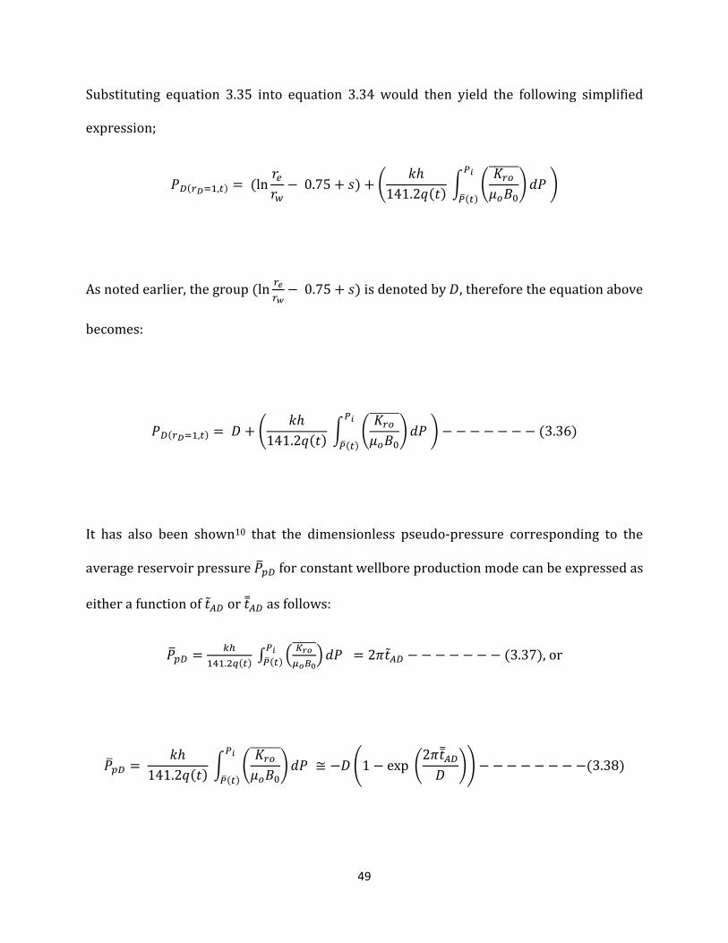
Substituting equation 3.35 into equation 3.34 would then yield the following simplified

expression;

��U´i$,�� ln 0�0� � 0.75 # F� # % T\141.2�� ; % wUJVJI?( �� A

A�� (

As noted earlier, the group �ln U�Ux � 0.75 # F� is denoted by �, therefore the equation above

becomes:

��U´i$,�� # % T\141.2�� ; % wUJVJI?( �� A

A�� ( � � � � � � � �3.36�

It has also been shown10 that the dimensionless pseudo-pressure corresponding to the

average reservoir pressure �� for constant wellbore production mode can be expressed as

either a function of �̃z� or �|z� as follows:

�� r�$�$.5@�� 3 ®�t�¯°4 �� A A�� 2��̃z� � � � � � � � �3.37�, or

�� T\141.2�� ; % wUJVJI?( �� A

A�� 1 � exp %2��|z�� (� � � � � � � � ��3.38�

50

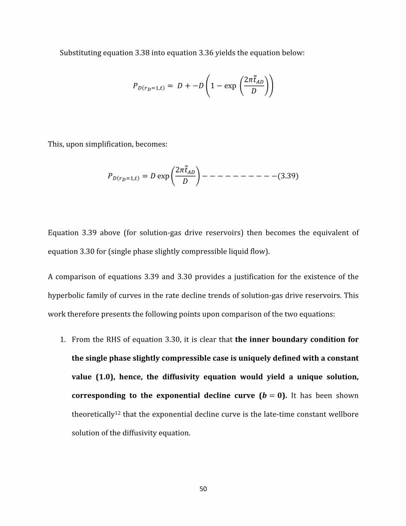
Substituting equation 3.38 into equation 3.36 yields the equation below:

��U´i$,�� # �� 1 � exp %2��|z�� (�

This, upon simplification, becomes:

��U´i$,�� exp %2��|z�� ( � � � � � � � � � ��3.39�

Equation 3.39 above (for solution-gas drive reservoirs) then becomes the equivalent of

equation 3.30 for (single phase slightly compressible liquid flow).

A comparison of equations 3.39 and 3.30 provides a justification for the existence of the

hyperbolic family of curves in the rate decline trends of solution-gas drive reservoirs. This

work therefore presents the following points upon comparison of the two equations:

1. From the RHS of equation 3.30, it is clear that the inner boundary condition for

the single phase slightly compressible case is uniquely defined with a constant

value (1.0), hence, the diffusivity equation would yield a unique solution,

corresponding to the exponential decline curve (¤ � Á). It has been shown

theoretically12 that the exponential decline curve is the late-time constant wellbore

solution of the diffusivity equation.

51

2. From the RHS of equation 3.39, it is clear that the inner boundary condition for

the solution-gas drive reservoir is not uniquely defined (even for a given

reservoir model); rather the expression is a function of fluid properties,

% |̈ÂÃ � Ä 3ÅÆ�¨�ÇÆ�¨�4( . Hence, solving the diffusivity equation with equation 3.39 as

the inner boundary condition would yield a family of curves (hyperbolic

family: Á " � , È. Á) with each member of the family (a given value of ¤) only

uniquely defined for a unique fluid model. In summary, this work is submitting

that the hyperbolic behavior of solution-gas drive reservoirs is a direct consequence

of the inner boundary condition (constant wellbore pressure) of the dimensionless

diffusivity equation for solution-gas drive reservoirs.

3. From the foregoing, it is clear that the ratio �S��X�� would be a significant determinant

of the value of � for a given reservoir/fluid model. This observation here is in

consonance with results published by Gentry and McCray6 showing that the relative

permeability characteristics have a significant influence on the parameter�. This is

also in agreement with the expression for � parameter presented by reference 10.

This mathematical justification for the existence of the hyperbolic curves in solution-gas

drive reservoirs is a major contribution of this work. The significance of this derivation

here (equation 3.39) as well as the observations made lies in its ability to pave way for

future efforts towards theoretically generating the complete Arp’s type curves.

52

CHAPTER 4

SIMULATION AND COMPUTATIONAL

PROCEDURES

A number of theories as well as deductions have been developed in this work as reported

in chapter three. In order to verify these theories and deductions, the need arose for a

comprehensive set of synthetic data (reservoir, fluid and historical production data)

required for such verification. The decision to employ synthetic data in the verification

became necessary due to scarcity of comprehensive real life data that will include all the

parameters required; more so, using synthetic data offered the possibility of performing

sensitivity analysis on some key parameters.

The first part of this chapter therefore presents the static reservoir/fluid properties which

essentially constituted the raw data fed into the simulator. The second part of this chapter

presents the simulation workflow with which the synthetic data were generated.

Furthermore, it was not possible to obtain direct outputs of some required parameters

from simulation runs, such parameters were however computed from simulation results.

The last part of this chapter presents details of such computations.

53

4.1 RESERVOIR AND FLUID DATA SET

The reservoir and fluid data set employed in this work is essentially the same as that

published in reference 10; this is done in order to avail the opportunity of comparing

results from this work with results from previous investigations. However, since the focus

of this work is based on sound theoretical considerations, the conclusions therein do not

depend on the specific data used.

Basically, a saturated, homogeneous, bounded, cylindrical reservoir is considered; a single

fully penetrating well producing at constant wellbore pressure (critical bottomhole

pressure �� ) is located at the center of the reservoir. The table below shows the details of

the reservoir properties.

Table 4.1: Reservoir Properties Data Set

Reservoir Properties Values

Drainage Radius, re (ft) 2624.672

Porosity, [, (fraction) 0.3

Permeability, K, (mD) 10

Well Radius, rw (ft) 0.32808

Initial Pressure = Bubble Point Pressure, Pi = Pb, (psi) 5704.78

Skin Factor, s 10

Initial Water Saturation, Swi (fraction) 0.3

Initial Compressibility, cti, psi-1 0.00001085

Initial Oil Viscosity, μoi cp 0.298

Thickness, h, (ft) 15.55

Critical Bottom Hole Pressure Constraint, Pwf (psi) 1696

54

The table below shows the oil PVT properties at various pressure nodes, the same data is

shown in the plots that follow:

Table 4.2: Oil PVT Properties Data Set

Pressure, P (psi)

Solution GOR, Rs

(MCF/STB) Bo (RB/STB) Oil Viscosity (cp)

100 0.0100 1.0622 1.3957

200 0.0263 1.0650 1.3525

300 0.0427 1.0683 1.3104

400 0.0594 1.0721 1.2695

500 0.0763 1.0765 1.2296

600 0.0933 1.0814 1.1909

700 0.1107 1.0868 1.1532

800 0.1282 1.0926 1.1165

900 0.1460 1.0990 1.0809

1000 0.1641 1.1059 1.0463

1500 0.2588 1.1469 0.8882

2000 0.3617 1.1984 0.7534

2500 0.4739 1.2593 0.6400

3000 0.5969 1.3284 0.5462

3500 0.7318 1.4044 0.4702

4000 0.8800 1.4864 0.4101

4500 1.0428 1.5731 0.3640

5000 1.2214 1.6633 0.3300

5500 1.4172 1.7558 0.3063

5704.78 1.5026 1.7941 0.2992

55

Figure 4.1: Oil PVT Properties (Solution GOR, Oil Formation Volume Factor and Oil Viscosity)

The table and the plots below show the Gas PVT properties at various pressure nodes.

Table 4.3: Gas PVT Properties Data Set

Pressure P (psi) Gas FVF, Bg (RB/MCF) Gas Viscosity μg (cp)

100 3.86E+001 0.010443

200 1.80E+001 0.010786

300 1.15E+001 0.011129

400 8.39E+000 0.011472

500 6.57E+000 0.011815

600 5.37E+000 0.012158

700 4.54E+000 0.012501

800 3.92E+000 0.012844

900 3.44E+000 0.013187

1000 3.06E+000 0.013530

1500 1.96E+000 0.015245

2000 1.43E+000 0.016960

2500 1.12E+000 0.018675

3000 9.15E-001 0.020390

3500 7.72E-001 0.022105

4000 6.67E-001 0.023820

4500 5.86E-001 0.025535

5000 5.22E-001 0.027250

5500 4.70E-001 0.028965

5704.78 4.51E-001 0.029667

0.00

0.20

0.40

0.60

0.80

1.00

1.20

1.40

1.60

1.80

2.00

0 2000 4000 6000

Rs

(MC

F/S

TB

), B

o (

RB

/ST

B),

μo

(cp

)

Pressure, P (psi)

Oil PVT Properties (Rs, Bo, μo)

Oil Formation

Volume

Factor, Bo

Oil Viscosity, μ

Solution

GOR, Rs

56

Figure 4.2: Gas PVT Properties (Gas FVF, Gas Viscosity)

Additionally, the simulation required values of undersaturated oil compressibility at the

pressure nodes indicated in the PVT tables above. The compressibility values were

computed using the Vasquez-Beggs57 correlation as shown below:

HJ � 5CD� # 17.2�É � 1,180ÊQ # 12.61ÊzAË � 1,43310��

The following values of indicated parameters are employed in computing the

compressibility data.

C�F�0E�.0 ��p�0��Ì0� � �É � 220j

O�F Í0�E.�Î � ÊQ � 0.65

Ï.) Í0�E.�Î � ÊzAË � 45.5

0.000

0.005

0.010

0.015

0.020

0.025

0.030

0.035

0.0

5.0

10.0

15.0

20.0

25.0

30.0

35.0

40.0

45.0

0 1000 2000 3000 4000 5000 6000

Ga

s V

isco

sity

μg

(cp

)

Ga

s F

VF

, B

g (

RB

/MC

F)

Pressure, P (psi)

Gas PVT Properties (Bg, μg)

Gas FVF, Bg

Gas Viscosity, μg

57

The table below shows the computed compressibility data.

Table 4.4: Undersaturated Oil Compressibility Data Set

Pressure, P (psi)

Solution GOR, Rs

(MCF/STB)

Undersaturated Oil

Compressibility (psi-1

)

100 9.9967 3.64E-004

200 26.2638 1.86E-004

300 42.7214 1.27E-004

400 59.3801 9.72E-005

500 76.2500 7.94E-005

600 93.3415 6.76E-005

700 110.6650 5.92E-005

800 128.2306 5.29E-005

900 146.0489 4.80E-005

1000 164.1300 4.41E-005

1500 258.8400 3.26E-005

2000 361.6700 2.70E-005

2500 473.9100 2.38E-005

3000 596.8500 2.19E-005

3500 731.7800 2.07E-005

4000 879.9900 2.00E-005

4500 1042.7700 1.96E-005

5000 1221.4100 1.94E-005

5500 1417.2000 1.94E-005

5704.78 1502.6372 1.95E-005

The relative permeability characteristics of the reservoir/fluid model considered is

displayed in the figure below. These relative permeability curves were however

approximated as straight line functions in the simulations and computations in this work.

58

Figure 4.3: Relative Permeability Characteristic Curves

4.2 SIMULATION DATA DECK AND RUN SPECIFICATIONS

The reservoir simulation software ECLIPSE 100 was employed in running the simulations

in this work. This section gives details of the ECLIPSE data deck as well as various run

specifications implemented in the simulation runs.

4.2.1 Simulator Data Deck

The various raw data shown above were presented in a text file in a format compatible

with ECLIPSE input data format. Various run specifications as well as output requests were

0.00

0.10

0.20

0.30

0.40

0.50

0.60

0.70

0.80

0.00 0.20 0.40 0.60 0.80 1.00

kro

, k

rg

Oil Saturation, So

Relative Permeability Characteristics

Oil Relative

Permeability, kro

Gas Relative

Permeability, krg

59

also specified in the text file using the relevant ECLIPSE keywords. The content of the input

data deck is presented in Appendix of this report.

4.2.2 Simulation Specifications and Controls

The following specifications and control parameters as required by the simulator were

specified:

1. Well Control: The well was initially placed on a constant oil rate control (peak rate)

until the bottomhole pressure dropped to the critical value of Pwfc at which point the

control was switched to BHP control in order to create the effects of a declining oil

well.

2. Peak Rate: The peak rate (rate at onset of decline) which is a measure of the

reservoir/wellbore capacity was set at 70% of the absolute open flow rate as

suggested by Fraim and Wattenbarger50

3. Economic Limit: An oil rate economic limit of 50STB/D was implemented to

terminate the simulation as soon as this limit is violated.

4. Non-Darcy Coefficient: The value for the non-Darcy coefficient, !, for the well was

calculated using the expression54 given below and fed into the simulator

! � 2.715 � 10�$��Ð�D�wV�D�\0�

Also, the following expression for gas density (g/cm3) at standard condition is

presentted59

60

oD� � 1.4935 � 10�l �D�Ð�D�

Combining the two equations above;

! � 2.715 � 10�$��oD�w1.4935 � 10�lV\0�

The turbulence factor � was computed using the Geertsma correlation58 shown

below

� � �¢�$$£Ñ.Ñ°.Ñ

4.2.3 Output Requests

The following output parameters were requested to be reported at each time step of the

simulation:

1. Field oil production rate (STB/D)

2. Field gas production rate (MCF/D)

3. Field cumulative oil produced (STB)

4. Field cumulative gas produced (MCF)

5. Field free gas production rate (MCF/D)

6. Field solution gas production rate (MCF/D)

7. Field GOR (MCF/STB)

8. Well bottomhole pressure, BHP, (psi)

9. Field average oil saturation

10. Field average gas saturation

11. Field average reservoir pressure (psi)

12. Fraction of oil rate due to solution-gas drive mechanism

13. Fraction of oil rate due to gas-cap influx

61

The last two parameters were requested in order to ascertain the reservoir is actually

producing due to solution-gas drive mechanism. Simulation results showed that the

fraction of oil produced due to solution-gas drive was approximately 1.0 throughout the

producing time. The output parameters listed above formed the basis for the computations

presented in the last section of this chapter. The time step for the simulation run as well as

the output reporting was set for an interval of one month; however, in order to accurately

capture the exact time of the onset of the decline, the month corresponding to the start of

decline was expanded into its constituent days so that the simulator’s output for this month

was reported in daily interval thereby capturing the exact day corresponding to onset of

decline. It was observed that this effort improves the results.

4.2.4 Simulation Initial Solution

In order to verify the correctness of the reservoir/fluid model fed into the simulator, a

request for the initial solution of the simulation run was incorporated. This was deemed

necessary so as to obtain the simulator’s result for initial fluid in place (oil in place, gas in

place and water in place). The simulator’s output for fluid in place was found to agree with

values calculated using simple volumetric formulae for fluid in place calculations.

62

4.3 COMPUTATIONAL PROCEDURES

It was not possible to obtain direct outputs of some parameters required to verify the

various theories developed in this work from simulation runs. Such parameters which are

essentially the total compressibility and mobility terms (and the various derivatives

needed to compute them) were however computed from simulation results using relevant

equations. This part of this chapter presents details of such computations.

To employ either of the equations presented in chapter 3 to compute �� 0 �� values,

the total compressibility term HS{ and the total mobility term X{ are defined as follows10:

HS{ � � LJIJ�� b�IJ�� IQ�� CD�� c � LQIQ�� b�IQ�� c � � � ��4.1�

X{ � r®��h��t��A� # r®³�h³�t³�A� � � � � � �4.2�

The detailed computational procedures required for various terms in equations 4.1 and 4.2

above and the eventual computation of �� 0 �� as a function of time is herein

presented.

1. Time (t), average pressure (�), average saturations�LJ �*� LQ ) data were obtained

from the simulator output file.

63

2. The PVT data ÒIJ��, IQ��, CD��Ó as functions of time were evaluated at average

reservoir pressure using the curve-fitting functions generated from the raw input

data.

3. The derivatives (wrt �� of the PVT data 6-¯��A�-A � IJÔ , -¯³�A�-A � IQÔ , -ÕÖ�A�-A � CDÔ 7 as

functions of time were computed using the following numerical derivative algorithm

�IJ�� IJÔ � %IJ�� IJ��$�� $� ( N��±$� � ��P # %IJ��±$� � IJ��±$� � �� ( N�� $�P��±$� � ��$� � � � �4.3�

�IQ�� IQÔ � %IQ�� IQ��$�� $� ( N��±$� � ��P # %IQ��±$� � IQ��±$� � �� ( N�� $�P��±$� � ��$� � � � �4.4�

�CD�� CDÔ � %CD�� CD��$�� $� ( N��±$� � ��P # %CD��±$� � CD��±$� � �� ( N�� $�P��±$� � ��$� � � � �4.5�

In the scheme above, index i referred to current time step while i+1 and i-1 referred to next

and previous time step respectively.

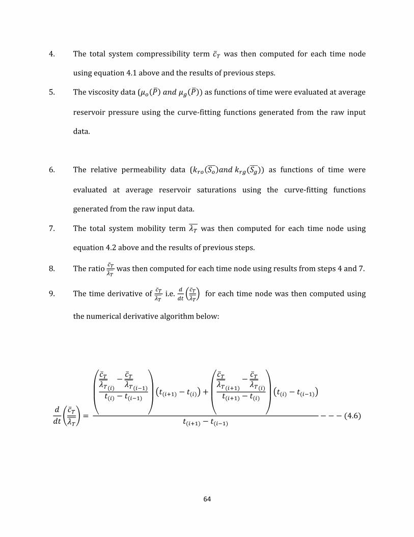
64

4. The total system compressibility term HS{ was then computed for each time node

using equation 4.1 above and the results of previous steps.

5. The viscosity data (VJ�� *� VQ�� as functions of time were evaluated at average

reservoir pressure using the curve-fitting functions generated from the raw input

data.

6. The relative permeability data (TUJ�LJ��*� TUQ�LQ�� as functions of time were

evaluated at average reservoir saturations using the curve-fitting functions

generated from the raw input data.

7. The total system mobility term X{ was then computed for each time node using

equation 4.2 above and the results of previous steps.

8. The ratio �S�� was then computed for each time node using results from steps 4 and 7.

9. The time derivative of �S�� i.e.

--� 3�S��4 for each time node was then computed using

the numerical derivative algorithm below:

�� %HS{X{( � ×ØÙHS{X{�� HS{X{��$�� $� ÚÛ

Ü N��±$� � ��P #×ØÙHS{X{��±$� � HS{X{��±$� � �� ÚÛ

Ü N�� $�P��±$� � ��$� � � � �4.6�

65

10. Lastly, the theoretical values of b, i.e. �� 0 ��, for each time node were then

computed using either equation 3.2 or 3.29 presented in chapter 3.

The results of the simulations and the computations that followed as well as the

verifications of the various theories developed in chapter 3 and the relevant discussions is

the focus of chapter five of this report.

66

CHAPTER 5

VERIFICATION OF THEORIES AND RESERVOIR

PROPERTY ESTIMATION

The derivation of a functional relationship between the empirical domain and the

theoretical domain of the decline parameter �� EF �� which is the foremost

contribution of this work has been presented in chapter three alongside other theories and

deductions developed. The details of the simulations and computational procedures

employed in generating data and parameters needed for the verification of the theories has

also been presented in chapter four. This chapter therefore presents the simulation results

as well as the results of the verification attempts. Theoretical justifications for observed

trends in the results are also presented in this chapter. In addition, a newly proposed

reservoir property estimation technique being a major contribution of this work is herein

presented with specific examples. Finally, analyses on the sensitivity of the results to some

key parameters were performed and reported in this chapter.

67

5.1 THEORETICAL DECLINE PARAMETER TREND THROUGH TIME

The reservoir and fluid properties for the base case has been presented in chapter three.

Also, the various simulation controls and specifications have been presented in chapter 4.

Presented in the figure below is the simulation result namely the oil flowrate through time

as well as the solution-gas drive index.

Figure 5.1: Base Case Production History: Rate-Time and Solution Gas Drive Index

The result above shows the dominance of solution-gas drive mechanism in the production.

Furthermore, the slight upward curvature of the semilog rate-time plot confirms the

0

0.1

0.2

0.3

0.4

0.5

0.6

0.7

0.8

0.9

1

1

10

100

1000

0 500 1000 1500 2000 2500 3000

So

luti

on

-Ga

s D

riv

e I

nd

ex

, S

GD

I

Oil

Pro

du

ctio

n R

ate

, q

(S

TB

/D)

Time, t (Days)

Production History: Rate-Time and Solution-Gas

Drive Index

Rate-Time Solution-Gas Drive Index

68

presence of hyperbolic rate decline; as suggested in reference 4. The results also show a

short constant (peak) rate production phase before decline sets in at day 12.

Using the simulators outputs (oil flowrate, average reservoir pressure and saturation as

functions of time) and employing various computational schemes presented in chapter

four, values for the theoretical decline parameter �� were computed as a function of time

using equation 3.2. Below is a plot of �� values with time. It should be noted that the time

item in the plot below refers to time elapsed since onset of decline, i.e. time � � 0

corresponds to start of decline.

Figure 5.2: Base Case: Theoretical �� Trend through Time

0

1

2

3

4

5

6

7

0 500 1000 1500 2000 2500 3000

bth

Time, t (days)

Theoretical bth Trend through Time

69

5.2 THEORETICAL JUSTIFICATION FOR THE DECLINE PARAMETER TREND

From figure 5.2 above, it is clear that the �� ranges from values greater than 1.0 to values

as low as 0.33. As a precursor to the explanations offered below for the various intervals of

values, the theoretical values, ¤¨© may be seen as reflecting the actual dynamics of the

reservoir and the fluid interaction through time; hence it may be expected to have a

dynamic (unstable) behavior through time. Below is the theoretical explanations offered by

this work for the various intervals of values of ¤¨©.

1. ¤¨© > 1.0: Transient Rate Decline Regime

This range of values may be attributed to transient rate decline, i.e. a decline

period during which the well is yet to feel the external boundary of the drainage

area. Various researchers10,12,13 have suggested that rate data existing in the

transient period will yield values of exponent b greater than 1.0. As evidence in

support of this proposition, results presented in the sensitivity analysis section

of this report showed that this range of values vanished for cases that precluded

transient rate decline.

2. 1 >¤¨© >0.67: Transition Decline Regime

Empirical surveys 10,12,13 of solution gas drive reservoirs performance has shown

that the exponent b should range from 0.33 to 0.67. However, it may be expected

there should be a sort of transition regime between the transient decline regime

(�� > 1.0) and the boundary-dominated empirically established regime (0.67

>�� > 0.33). In other words, the values between 1.0 and 0.67 in the above plot

70

may be seen as representing a transition from transient rate decline regime to

boundary-dominated rate decline regime. Similar to the transient rate decline

regime, results presented in the sensitivity analysis section of this report

showed that this range of values vanished for cases where only boundary-

dominated rate decline is ensured.

3. 0.67 >¤¨© > 0.33: Boundary-dominated Solution-gas Drive Decline Regime

The values in this range should represent the actual boundary-dominated

solution-gas drive decline behavior. This fact could be supported by the fact that

the reservoir exhibited this range of values for the longest period of the decline

time.

4. ¤¨© < 0.33: Approaching Slightly-compressible Liquid Production

Some cases considered and reported in later sections of this report exhibited a

range of ¤¨© values less than 0.33. These values are below the lower limit of the

empirically expected range for solution gas drive reservoirs. It may be expected

that as the reservoir loses more of the solution gas due to production, its

behavior starts to approach that of a slightly compressible liquid single phase

flow. Single-phase slightly compressible liquid flows are known theoretically to

decline exponentially, i.e. b = 0.4,3 Hence, as the reservoir approaches the single

phase flow behavior, the �� values are seen to be less than 0.33 and are

approaching zero.

71

The propositions above as regards the theories of rate decline in solution-gas drive

reservoirs has not been presented previously and is therefore a significant contribution of

this work.

5.3 EFFECT OF INCORPORATING NON-DARCY FLOW

Camacho and Raghavan10 had expressed hopes that the incorporation of near wellbore

non-Darcy flow effects into the theoretical developments of rate decline in solution-gas

drive reservoirs could yield constant values of �� throughout decline time. In order to

verify this anticipation for constant �� values, this work derived a new expression

(equation 3.29) for �� as function of physical reservoir and fluid properties using similar

formulation as in reference 10 but incorporating the rate-dependent skin factor

representing the non-Darcy flow effects. The derivation is presented in chapter three of

this report. Values of �� (theoretical decline parameter with consideration for non-

Darcy flow) computed using equation 3.29 is presented in the plot below on the same axes

with values of �� for comparison.

72

Figure 5.3: Base Case: Theoretical �� and �� through Time

From figure 5.3 above, it is evident that the decline parameter with consideration for non-

Darcy effects, �� vary through time much same way as the decline parameter without

consideration for non-Darcy effects, precluding any expectation for constant values of

�� through time.

If the propositions about the dynamic behavior of the decline parameter as being presented

by this work are valid, then the �� values may never exhibit any constancy in spite of

considerations for non-Darcy flow effects. The ¤¨©�ÝÃ values will rather be expected to

reflect the dynamics (through time) of the reservoir and fluid interactions (mobility and

compressibility characteristics). System mobility (relative permeability and viscosity) as

well as compressibility (PVT) in solution gas drive reservoirs are known to be functions of

average reservoir pressure and saturation30 which change with time due to production.

0

1

2

3

4

5

6

7

0 500 1000 1500 2000 2500 3000

bth

Time, t (days)

Theoretical bth and bth-nD Trend through Time

bth

bth-nD

73

The empirical exponent b has been related to the popular back-pressure curve exponent4

denoted as n. Fetkovich32 had attributed exponent n values less than unity to non-Darcy

flow. Camacho and Raghavan52 also published results that substantiated Fetkovich’s claim.

However, Fetkovich32 submitted that n values can be less than unity strictly as a result of

variation in fluid properties. As a matter of fact, Camacho and Raghavan52 suggest that n

values will generally vary with time unless the variation is completely counteracted with

the non-Darcy flow effects. However, non-Darcy flow coefficients in solution gas drive

reservoirs are rather very small in values (1.7107 X 10-6 D/MCF) for the reservoir/fluid

model considered here) and may never measure up to values sufficient to counteract the

variation due to changes in fluid properties. The results reported in this current work and

its emerging propositions confirm the positions already established in literatures.

5.4 VERIFICATION OF DERIVED RELATIONSHIP

A major contribution of this work is the derivation of a functional relationship between the

empirical domain and the theoretical domain of the decline parameter�� EF �� . This

relationship is reported in chapter three as equation 3.8 and is presented below for

convenience.

1�� N�� JP � ��> � � � � � � � � � ��3.8�

74

As a corollary, the LHS of equation 3.8 was also represented as a function of physical

reservoir and fluid properties in equation 3.9

1�� N�� JP � 2�0.006328T[]� X{HS{ � � � � � � � � � ��3.9�

Equation 3.8 represents the empirical domain of the decline parameter while equation 3.9

represents the theoretical domain.

From the two equations above, it is expected that the right hand side quantity (RHS) of

both equations should be equal since the left hand side (LHS) is essentially equal.

The equality (at least in the approximate sense) of the RHS of both equations 3.8 and 3.9

was verified using simulation results; rate-time data, to compute � �*� �� and

employing the various computational schemes presented in chapter four to compute X{

and HS{ . The result of the verification attempt is presented below as a plot of the RHS of both

equations with time.

75

Figure 5.4: Base Case: Verification of Equations 3.8 and 3.9

The following features of the plot are here highlighted.

1. The two curves exhibit similar trends over time.

2. The initial agreement between the two curves may be taken as a pseudo

agreement since the empirical domain could not exist until there be sufficient

production decline history

3. The discrepancy between the two curves, although initially grew large,

narrows down with time. As a matter of fact, the discrepancy is expected to

become insignificant if the simulation is extended; here the simulation stops

because the economic limit (50 STB/D) constraint imposed has been

violated.

0

0.0002

0.0004

0.0006

0.0008

0.001

0.0012

0.0014

0 1000 2000 3000

RH

S o

f E

qu

ati

on

8,

9

Time, t (days)

Verification of equations 3.8 and 3.9

Equation 3.9:

Theoretical

Equation 3.8:

Empirical

76

4. Point 3 above suggests the equality of the two equations above would be

improved as more and more historical production decline data becomes

available.

5. At the end of the simulation time, the relative discrepancy has reduced to

only 7.7%.

5.5 PROPOSED RESERVOIR PROPERTY ESTIMATION TECHNIQUES

5.5.1 Reservoir Permeability Estimation: Procedure and Application.

Consequent upon the verification of the equality of equation 3.8 and 3.9 (at least in an

approximate sense), this current work therefore proposed a new improved technique for

estimating reservoir permeability using historical field data. The basis for this proposed

technique, derived by equating the RHS of equation 3.8 and 3.9 and solving for reservoir

permeability T was presented as equation 3.11 in chapter three and is repeated here for

convenience.

T � ��>[]�2�0.006328 HS{X{ � � � � � � � � � ��3.11�

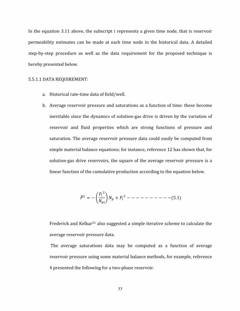
77

In the equation 3.11 above, the subscript . represents a given time node, that is reservoir

permeability estimates can be made at each time node in the historical data. A detailed

step-by-step procedure as well as the data requirement for the proposed technique is

hereby presented below.

5.5.1.1 DATA REQUIREMENT:

a. Historical rate-time data of field/well.

b. Average reservoir pressure and saturations as a function of time: these become

inevitable since the dynamics of solution-gas drive is driven by the variation of

reservoir and fluid properties which are strong functions of pressure and

saturation. The average reservoir pressure data could easily be computed from

simple material balance equations; for instance, reference 12 has shown that, for

solution-gas drive reservoirs, the square of the average reservoir pressure is a

linear function of the cumulative production according to the equation below.

�5 � � %��5!�( ! # ��5 � � � � � � � � � ��5.1�

Frederick and Kelkar51 also suggested a simple iterative scheme to calculate the

average reservoir pressure data.

The average saturations data may be computed as a function of average

reservoir pressure using some material balance methods, for example, reference

4 presented the following for a two-phase reservoir.

78

LJ � �1 � L�� &1 � !! ' & IJIJ�' � � � � � � � ��5.2�

5.5.1.2 PROCEDURES:

1. Acquire the required data as stated above.

2. From the rate-time data, using conventional curve-fitting methods or type-curve

matching, determine the values of the empirical decline parameters, � �*� ��.

3. Compute values of PVT data ÒIJ��, IQ��, CD��Ó at average reservoir pressure for

each time nodes. Curve-fitted functions of initial PVT data of the reservoir fluid may

be used for this computation at later times in the reservoir life.

4. Using the equation below, compute the total compressibility at each of the time

nodes. The derivatives in the equation may be computed using numerical

differentiation algorithms.

HS{ � � LJIJ�� b�IJ�� IQ�� CD�� c � LQIQ�� b�IQ�� c

5. Compute values of the relative permeability data ÒTUJ�LJ��*� TUQ�LQ�Ó at average

reservoir saturations for each time nodes. Curve-fitted functions of the core-derived

relative permeability data of the reservoir may be used for this computation.

79

6. Compute values of the viscosity data Ò�VJ�� *� VQ��Ó at average reservoir

pressure for each time nodes. Curve-fitted functions of initial viscosity data of the

reservoir fluid may be used for this computation at later times in the reservoir life.

7. Using the equation below, compute the total mobility at each of the time nodes.

X{ � TUJ�LJ�VJ�� # TUQ�LQ�VQ��

8. Substitute the results of the previous steps into equation 3.11 above to solve for

permeability estimates, T at each time node.

5.5.1.3 APPLICATION OF TECHNIQUE

The application of this proposed technique to the reservoir model considered in this

work yields excellent permeability estimates throughout time. The plot of the

permeability estimates through time is hereby presented below.

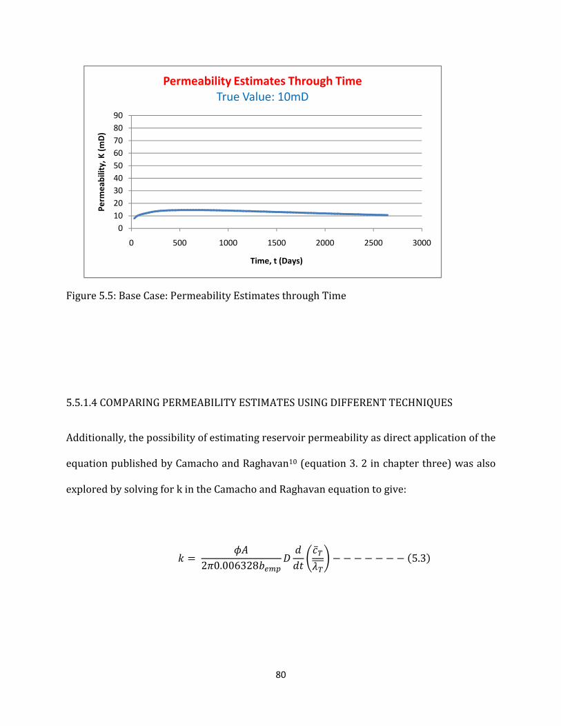
80

Figure 5.5: Base Case: Permeability Estimates through Time

5.5.1.4 COMPARING PERMEABILITY ESTIMATES USING DIFFERENT TECHNIQUES

Additionally, the possibility of estimating reservoir permeability as direct application of the

equation published by Camacho and Raghavan10 (equation 3. 2 in chapter three) was also

explored by solving for k in the Camacho and Raghavan equation to give:

T � []2�0.006328�� %HS{X{( � � � � � � � �5.3�

0

10

20

30

40

50

60

70

80

90

0 500 1000 1500 2000 2500 3000

Pe

rme

ab

ilit

y,

K (

mD

)

Time, t (Days)

Permeability Estimates Through Time

True Value: 10mD

81

The ‘permeability’ values through time computed using Camacho and Raghavan10 equation

(equation 5.3) is plotted alongside permeability values computed using the equation

proposed by this work (equation 3.11) and is shown below for comparison purposes.

Figure 5.6: Comparing Permeability Estimates using different Techniques

These results showed that the Camacho and Raghavan10 equation (equation 5.3) cannot be

utilized for permeability estimation purposes as it is done with the relationship presented

by this current work (equation 3.11). As a matter of fact, the ‘permeability’ values gotten

using Camacho and Raghavan equation varied very widely away from the true value. This is

because although the Camacho and Raghavan equation is theoretically correct, it does not

have any link with the empirical domain, rather, it based on the expectation that the

theoretical decline parameter �� is equivalent to the empirical decline parameter��;

theories and results reported in this work have shown that expectation does not have a

theoretical basis and as a matter of fact, the equivalence of �� *� ��does not exist.

0

10

20

30

40

50

60

70

80

90

0 1000 2000 3000

Pe

rme

ab

ilit

y,

K (

mD

)

Time, t (Days)


True Value: 10mD

This Work

Camacho/Raghavan

82

Hence the exponent �� on the LHS (of equation 3.2) cannot be taken as the equivalence of

the empirically determined exponent��. Instead, as presented by this work, the

equivalence between the empirical domain and the theoretical domain of the decline

parameter is anchored on a relationship between the empirical parameter �� and the

time-weighted average of the theoretical values��. This relationship has been derived in

this work and is a major contribution of this work. This relationship forms the basis for the

permeability estimation techniques being proposed by this work; hence the accuracy of the

technique.

5.5.2 Reservoir Radius (re) Estimation

Camacho and Raghavan10 had presented a form of the material balance equation for

solution-gas drive reservoir as given below:

�!�� !Ô � HS{Z[]\5.614 X{ � � � � � � � � � � � �5.4�

Where Z � r®��h��t��A�¯��A� and ] � �0�5

Solving for the reservoir/drainage radius 0� in the above equations yields

0� � Þ5.614!ÔX{HS{Z[�\ � � � � � � � � � ��5.5�

83

As a direct application of the Camacho and Raghavan10 work, equation 5.5 was employed in

estimating the drainage radius for the reservoir model considered in this work. Excellent

estimates of the reservoir drainage radius were obtained as shown in the plot of reservoir

radius estimates through time below.

Figure 5.7: Base Case: Reservoir Radius (re) Estimates through Time

5.6 SENSITIVITY ANALYSIS

The following analyses were performed with the aim of establishing the effect of changing

some key parameters on the results outlined in this work. In each case, the value for a

parameter is changed and the result is compared to the base case.

0

500

1000

1500

2000

2500

3000

0 500 1000 1500 2000 2500 3000

Re

serv

oir

Ra

diu

s, r

e(f

t)

Time, t (Days)

Reservoir Radius (re) Estimates Through TimeTrue Value :2624.672

Max. Error: 15.5% Min. Error: 0.01%

84

5.6.1 Case 1: Effect of Critical Gas Saturation

In the base case, the critical gas saturation at which gas becomes mobile in the reservoir is

set at zero; i.e. LQ� � 0. In this case however, the critical gas saturation was set at 5% i.e.

LQ� � 0.05. Below is the plot of the simulator output for case 1.

Figure 5.8: Case 1: Production History: Rate-Time and Solution-gas Drive Index

The result presented above exhibits trends similar to the result for the base case. However,

in this case, the decline phase started after 29 days as against the base case where the

decline phase started just after 12 days. The delay of the onset of decline in this case is

explained thus:

1. In case 1, due to the non-zero value assigned to the critical gas saturation, it is

expected that free gas flow in the reservoir is delayed until gas saturation attained

the critical value. Hence as gas solution-gas evolves out of solution and is retained

0

0.2

0.4

0.6

0.8

1

1

10

100

1000

0 1000 2000 3000 4000 So

luti

on

-Ga

s D

riv

e I

nd

ex

, S

GD

I

Oil

Pro

du

ctio

n R

ate

, q

(S

TB

/D)

Time, t (Days)

Production History: Rate-Time and Solution-gas

Drive Index

Rate-Time Solution-gas Drive Index

85

due to its immobility, the gas expands and therefore helps to maintain pressure in

the reservoir thereby delaying the attainment of the critical bottomhole pressure

�� due to pressure drop. Decline phase can only start when bottomhole pressure

drops to its lowest permissible, �� .

2. The trend noticed in the gas-oil ratio (GOR) plots for the two cases (base case and

case 1) also lend evidence to the delayed decline phase.

Figure 5.9: Producing Gas-Oil Ratio, GOR Trend: Base Case and Case 1

In the plots above, only the values for the first year of production decline is shown;

this is done so as highlight the major difference in the plot which occurs at the

beginning of decline phase.

From the plots, it is observed that for case 1, the GOR value reached its lowest and

picked up at 27 days while decline started at 29 days. On the other hand, for the

base case, the GOR value reached its lowest and picked up at 8 days while decline

0

1

2

3

4

5

6

7

0 100 200 300 400

Pro

du

cin

g G

as-

oil

Ra

tio

, G

OR

(MC

F/S

TB

)

Time, t (days)

Producing Gas-oil Ratio GOR Trend: Base Case

and Case 1

Base Case

Case 1

86

started at 12 days. The point at which the GOR values started increasing

corresponds to the attainment of the critical gas saturation, LQ�. As the critical gas

saturation is attained, gas becomes mobile and the reservoir is deprived of pressure

maintenance, hence pressure drops quickly to the lowest permissible, �� .

Other results obtained for case 1 exhibits similar behavior to those in the base case. The

implication of this is that although the value of LQ� have the effect of altering the timing of

the onset of the decline phase, it has no significant effect on the accuracy of the

permeability estimates generated thereby.

Figure 5.10: Case 1: Theoretical �� Trend through Time

0

1

2

3

4

5

6

7

0 500 1000 1500 2000 2500 3000

bth

Time, t (days)


87

Figure 5.11: Case 1: Permeability Estimates through Time

5.6.2 Case 2: Effect of Permeability Value

The essence of this case study is to create a reservoir model that precludes the occurrence

of transient rate decline. It is expected that the higher the absolute permeability of the

reservoir rock, the faster the pressure transient travels outwardly from the wellbore

through the porous rock to the external boundary of the drainage area; hence the more the

likelihood of boundary-dominated flow setting in ahead of the onset of decline phase

thereby precluding transient rate decline. For this case, the absolute permeability of the

reservoir model was set at 100mD as against 10mD in the base case; also, to accommodate

the increased permeability, the peak rate was set at 1000STB/D as against 270STB/D in

the base case. Below are the results of this case study and the discussions.

0

20

40

60

80

100

120

0 500 1000 1500 2000 2500 3000

Pe

rme

ab

ilit

y,

K (

mD

)

Time, t (Days)


True Value: 10mD

This Work

Camacho/Raghavan

88


The results in this case run were found to conform to expectations as the �� values

reported were less than 1.0 thereby confirming the absence of transient rate decline. If

indeed the transient rate decline regime was absent, then it is only proper to expect that

the transition regime (between transient and boundary-dominated rate decline regimes)

be also absent. The results of this case study also confirmed the absence of the transition

decline regime since the transition interval 1 >�� >0.67 was absent. These results

therefore lend credence to the correctness of the theoretical justifications, offered by this

work, for the various intervals of �� values.

0

0.05

0.1

0.15

0.2

0.25

0.3

0.35

0.4

0.45

0 200 400 600 800 1000

bth

Time, t (days)


89


From, the plots above, it is observed that the accuracy of the permeability estimates is

similar to the accuracy observed in the base case; implying that the presence of transient

rate decline regime may not have any significant effect on the accuracy of the permeability

estimates.

5.6.3 Case 3: Effect of Reservoir Drainage Radius

As in case 2 above, the essence of this case study is to create a reservoir model that

precludes the occurrence of transient rate decline. It is expected that the smaller the well’s

drainage area, the sooner the pressure transient from the well reaches the external

boundary of the drainage area; hence the more the likelihood of boundary-dominated flow

setting in ahead of the onset of decline phase thereby precluding transient rate decline. For

this case, the external radius of the reservoir model was set at 1000ft as against 2624.672ft

0

20

40

60

80

100

120

140

0 500 1000

Pe

rme

ab

ilit

y,

K (

mD

)

Time, t (Days)


True Value: 100mD

This Work

Camacho/Raghavan

90

in the base case; also, to maintain the intended reservoir pore volume, the reservoir

thickness was set at 107ft as against 15.55ft in the base case. Below are the results of this

case study and the discussions.


The results in this case run were found to conform to expectations and also to trends

already established in case 2. The �� values reported were less than 1.0 thereby

confirming the absence of transient rate decline. The results of this case study also

confirmed the absence of the transition decline regime since the transition interval

1>��>0.67 was absent. These results together with those of case 2 therefore lend credence

to the correctness of the theoretical justifications, offered by this work, for the various

intervals of �� values. However, as shown in plot below, the accuracy of the reservoir

radius estimates is improved compared to the base case. The maximum error in this case is

2.5% while the minimum error is 0.002%; both values represent improvements over the

0

0.1

0.2

0.3

0.4

0.5

0.6

0.7

0 500 1000 1500

bth

Time, t (days)


91

corresponding values in the base case. This improvement is arguably due to the absence of

transient rate decline regime. Fetkovich et al13 had suggested that reservoir volume-related

properties should not be estimated using decline curve analysis (type curve matching)

before boundary-dominated flow fully exists. It may then be important to screen a given

rate-time data in order to eliminate any transient rate decline data points. Existing method

for determining the time for the start of boundary-dominated flow for multiphase

conditions50 involves the computation of various pseudo functions (integrals) that may not

be practical for this application. However, an approximation of the time at which the

pressure wave propagates to the reservoir boundary can be obtained by employing the

equation for radius of investigation for single phase condition.4

0��ß � 0.0325Þ T�[VH�

However, the equation above could only be used if there are estimates of both the

permeability and reservoir radius from other formation evaluation sources; in such case,

the equation above could be solved for �; being an approximation of the time for the start of

boundary-dominated flow.

92

Figure 5.15: Case 3: Reservoir Radius (re) Estimates through Time

5.6.4 Case 4: Effect of Critical Bottomhole Pressure

The essence of this case study is to investigate the effect of the critical bottomhole pressure

on the theoretical decline parameter, �� as well as on the permeability estimates. The

critical bottomhole pressure itself is a function of both the wellbore configuration and the

reservoir deliverability. In this case, the critical bottomhole pressure was set at 700psi as

against 1696psi in the base case. Results are shown below.

0

200

400

600

800

1000

1200

0 500 1000 1500

Re

serv

oir

Ra

diu

s, r

e(f

t)

Time, t (Days)

Reservoir Radius (re) Estimates Through Time

True Value :1000 ft


93


From the �� values in the plot above, it is observed that the transient rate decline regime

did not vanish in this case implying that the occurrence or otherwise of the transient rate

decline regime is less sensitive to the value of the critical bottomhole pressure of the

reservoir/wellbore model.

The accuracy of the permeability estimates is discussed next.

0

0.5

1

1.5

2

2.5

3

3.5

4

0 500 1000 1500 2000 2500 3000 3500

bth

Time, t (days)


94


From the plot above, it is observed that the permeability estimates in this case study are

less accurate when compared to the estimates in the base case. The reduced accuracy,

when considered side-by-side with the reduced agreement between the empirical domain

and the theoretical domain, reveals an interesting trend discussed here. It is noticed that

the lowest value of �� recorded is about 0.4; this suggests the condition in the reservoir is

still far from being considered to be approaching single phase behavior i.e. the reservoir

has not yet exhausted the time span for the solution-gas decline regime. This fact is

arguably the reason for the reduced agreement between the empirical and the theoretical

curves even at field abandonment production rate as shown in the plots below. The

reduced agreement consequently affected the accuracy of the permeability estimates as

seen in the plot above. The implication of this is that the accuracy of the permeability

estimates depends on the availability of data that spans more and more period of the

solution-gas decline regime. The caution here however is that as soon as the entire time

0

10

20

30

40

50

60

0 500 1000 1500 2000 2500 3000

Pe

rme

ab

ilit

y,

K (

mD

)

Time, t (Days)


True Value: 10mD

This Work

Camacho/Raghavan

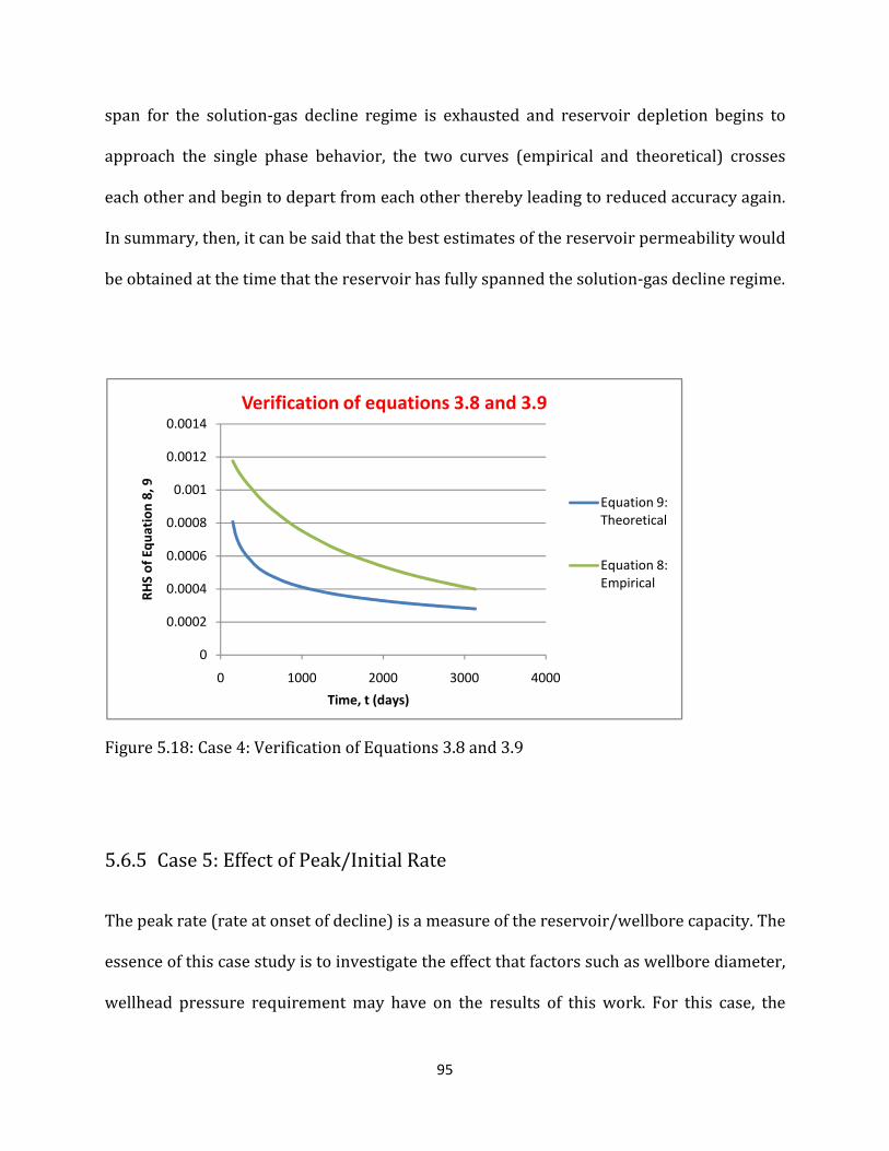
95

span for the solution-gas decline regime is exhausted and reservoir depletion begins to

approach the single phase behavior, the two curves (empirical and theoretical) crosses

each other and begin to depart from each other thereby leading to reduced accuracy again.

In summary, then, it can be said that the best estimates of the reservoir permeability would

be obtained at the time that the reservoir has fully spanned the solution-gas decline regime.

Figure 5.18: Case 4: Verification of Equations 3.8 and 3.9

5.6.5 Case 5: Effect of Peak/Initial Rate

The peak rate (rate at onset of decline) is a measure of the reservoir/wellbore capacity. The

essence of this case study is to investigate the effect that factors such as wellbore diameter,

wellhead pressure requirement may have on the results of this work. For this case, the

0

0.0002

0.0004

0.0006

0.0008

0.001

0.0012

0.0014

0 1000 2000 3000 4000

RH

S o

f E

qu

ati

on

8,

9

Time, t (days)


Equation 9:

Theoretical

Equation 8:

Empirical

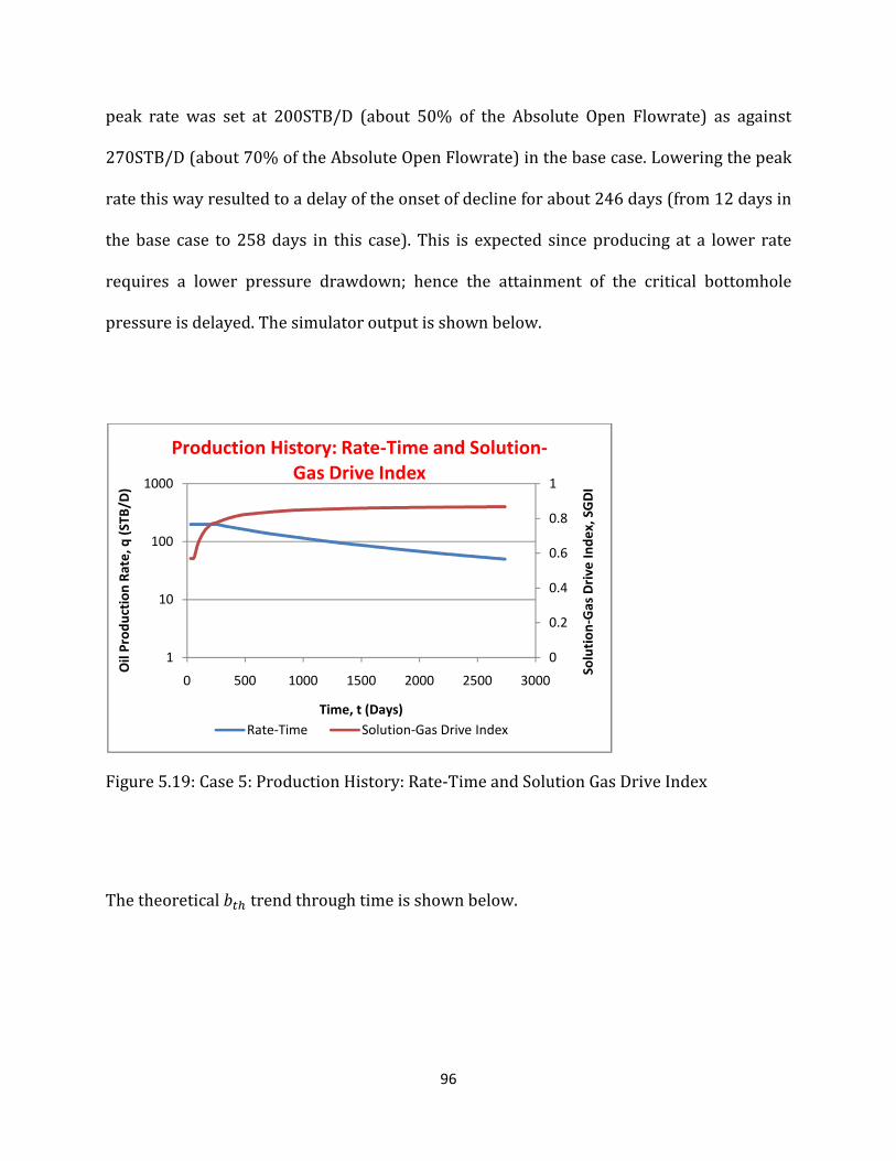
96

peak rate was set at 200STB/D (about 50% of the Absolute Open Flowrate) as against

270STB/D (about 70% of the Absolute Open Flowrate) in the base case. Lowering the peak

rate this way resulted to a delay of the onset of decline for about 246 days (from 12 days in

the base case to 258 days in this case). This is expected since producing at a lower rate

requires a lower pressure drawdown; hence the attainment of the critical bottomhole

pressure is delayed. The simulator output is shown below.

Figure 5.19: Case 5: Production History: Rate-Time and Solution Gas Drive Index

The theoretical �� trend through time is shown below.

0

0.2

0.4

0.6

0.8

1

1

10

100

1000

0 500 1000 1500 2000 2500 3000

So

luti

on

-Ga

s D

riv

e I

nd

ex

, S

GD

I

Oil

Pro

du

ctio

n R

ate

, q

(S

TB

/D)

Time, t (Days)

Production History: Rate-Time and Solution-

Gas Drive Index

Rate-Time Solution-Gas Drive Index

97


From the plot above it is observed that the maximum (and initial) value of the theoretical

�� was 1.88 as against 5.74 for the base case. This is arguably due to the delayed onset of

the decline phase. Since decline is delayed, it is expected that there will be less of transient

rate decline regime as the onset of decline could have occurred just before the beginning of

boundary dominated flow. This result suggest that the more transient rate decline regime

experienced by a well, the higher above 1.0 will be its initial �� values. This case also

recorded improved accuracy for both the permeability and the drainage radius estimates

as shown in the plots below. This improvement is considered to be due to the fact that

there is less of transient rate decline regime compared to the base case.

0

0.2

0.4

0.6

0.8

1

1.2

1.4

1.6

1.8

2

0 500 1000 1500 2000 2500 3000

bth

Time, t (days)


bemp = 0.612

98


Figure 5.22: Case 5: Reservoir Radius (re) Estimates through Time

0

5

10

15

20

25

30

35

0 1000 2000 3000

Pe

rme

ab

ilit

y,

K (

mD

)

Time, t (Days)


True Value: 10mD

This Work

Camacho/Raghavan

0

500

1000

1500

2000

2500

3000

0 500 1000 1500 2000 2500 3000

Re

serv

oir

Ra

diu

s, r

e(f

t)

Time, t (Days)

Reservoir Radius (re) Estimates Through Time

True Value: 2624.672 ft


99

5.6.6 Case 6: Effect of Reservoir Heterogeneity.

The essence of this case is to investigate the effect of reservoir (permeability and porosity)

heterogeneity on the results of the estimates technique presented by this work. Essentially,

one would like know to what extent would the permeability estimates be representative of

the permeability values of the different layers present in an heterogeneous reservoir. For

this case, the reservoir model as described in the base case was divided into two layers.

Heterogeneity was introduced into the reservoir by assigning different values of porosity

and permeability to different layers according to the grid data shown in the table below.

Two heterogeneous cases were considered in order to investigate not just the effect of

heterogeneity, but also the effect of the degree of heterogeneity. For the purpose of

comparison, the values of properties assigned to each heterogeneous case is such that the

thickness-weighted average permeability and the thickness-weighted average porosity is

still of the same values as the permeability and porosity values in the base case.

Table 5.1: Grid Data for Heterogeneous Case

Case 6a

Layer Thickness Layer Permeability Layer Porosity

Layer 1 8 150 0.35

Layer 2 7.55 50 0.25

Thickness-weighted Average 101.4469453 0.301446945

Case 6b

Layer Thickness Layer Permeability Layer Porosity

Layer 1 8 130 0.35

Layer 2 7.55 70 0.25

Thickness-weighted Average 100.8681672 0.301446945

100

The results for each of the two heterogeneous cases are presented in the plot below.

Figure 5.23: Case 6a: Verification of Equations 3.8 and 3.9

Figure 5.24: Case 6b: Verification of Equations 3.8 and 3.9

0

0.001

0.002

0.003

0.004

0.005

0.006

0.007

0 200 400 600 800 1000

RH

S o

f E

qu

ati

on

8,

9

Time, t (days)


Equation 9:

Theoretical

Equation 8:

Empirical

0

0.001

0.002

0.003

0.004

0.005

0.006

0 500 1000 1500

RH

S o

f E

qu

ati

on

8,

9

Time, t (days)


Equation 9:

Theoretical

Equation 8:

Empirical

101

The results above showed that generally, there is an agreement between the empirical and

the theoretical domains even for heterogeneous reservoirs. Furthermore, the results

showed that the degree of agreement reduces with increasing heterogeneity. Note that case

6a has a higher degree of permeability heterogeneity (layer 1: 150mD; layer 2: 50mD) than

case 6b (layer 1: 130mD; layer 2: 70mD).

The effect of the heterogeneity on the representativeness of the permeability estimates is

discussed with the permeability estimates plots shown below.

Figure 5.25: Case 6a: Permeability Estimates through Time

0

50

100

150

200

250

0 200 400 600 800 1000

Pe

rme

ab

ilit

y,

K (

mD

)

Time, t (Days)

Permeability Estimates Through TimeHigh Perm Layer: 150 mD Low Perm Layer: 50mD

Thickness-weighted Average Permeability: 100mD

This Work

Camacho/Raghavan

102

Figure 5.26: Case 6b: Permeability Estimates through Time

From the two heterogeneous cases shown in the plots above, it is observed that at early

times, the permeability estimates reflects the permeability value for the higher

permeability layer (150mD for case 6a and 130mD for case 6b); however, with time, the

permeability estimates reflects values approaching the thickness-weighted average of the

permeability values for all layers present (100mD for both cases).

0

20

40

60

80

100

120

140

160

180

0 200 400 600 800 1000

Pe

rme

ab

ilit

y,

K (

mD

)

Time, t (Days)

Permeability Estimates Through TimeHigh Perm Layer: 130mD Low Perm Layer: 70mD

Thickness-weighted Average Permeability = 100mD

This Work

Camacho/Raghavan

103

CHAPTER 6

CONCLUSIONS AND RECOMMENDATIONS

6.1 CONCLUSIONS

Previous attempts10 at establishing the theories of rate decline in solution-gas drive

reservoirs have yielded expressions relating the theoretical decline exponent �� to

reservoir/fluid properties. However, the values computed from such expression, although

theoretically sound, are not constant through time. More disturbing is the fact that the

values did not exhibit any equivalence with the empirically determined decline exponent,

��. This fact suggests there is a missing link between the theoretical and the empirical

domains of the decline curves analysis. This work has successfully provided the missing

link; expressed as a functional relationship between the empirical decline exponent,

��and the time-weighted average of the values of the theoretical decline exponent

known as ��. In addition, this work has developed a new improved reservoir permeability

estimation technique. The technique has been applied to a number of cases and found to

yield excellent estimates of reservoir permeability even for heterogeneous reservoirs.

Analyses have been performed on the sensitivity of the results to some key parameters.

104

Based on the results presented in this work, the following conclusions are warranted.

1. The theoretical decline exponent �� for a given reservoir/wellbore model varies

considerably through time, and may have values above 1.0

2. The theoretical decline exponent �� may be seen as reflecting the actual dynamics

of the reservoir and fluid interaction through production time; hence it may be

expected to have a dynamic (unstable) behavior through time.

3. Considering the various intervals of values present in a typical �� trend through

time, the following four distinct regimes of rate decline in solution-gas drive

reservoirs has been identified.

a. Transient rate decline regime: �� > 1.0

b. Transition rate decline regime: 1 >�� >0.67

c. Boundary-dominated Solution-gas drive decline regime: 0.67 >�� > 0.33

d. Approaching slightly compressible liquid single phase decline: �� < 0.33

Results presented in this work confirmed the presence of one more of these regimes in

a solution-gas drive reservoir depending on the reservoir/wellbore configuration.

4. The theoretical decline exponent, �� may never exhibit any constancy even with

considerations for non-Darcy flow effects as the non-Darcy flow coefficients in

solution-gas drive reservoirs are very small in values and may never measure up to

values sufficient to counteract the variation in �� due to changes in fluid properties.

5. The time-weighted average of �� values for a given reservoir/wellbore model is

related to the empirical decline exponent. The equation showing this relationship

has been derived and presented in this work.

105

6. Consequent upon the derivation of the relationship stated above, a new improved

technique for estimating reservoir permeability has been developed. The technique

yielded excellent estimates for reservoir permeability even for heterogeneous

reservoirs.

7. A technique for estimating a well’s drainage area was also presented. This technique

is based on the form of material balance equation for solution-gas drive presented

by Camacho and Raghavan10.

8. Although, the value of critical gas saturation LQ� has the effect of altering the timing

of the onset of decline, it has no significant effect on the accuracy of the permeability

estimates.

9. Reservoir with high permeability values may not exhibit the transient rate decline

regime as well as the transition rate decline regime; hence the ��intervals for these

regimes may be absent in such reservoirs.

10. The presence of transient rate decline regime has insignificant effect on the

accuracy of the permeability estimates.

11. The transient rate decline regime as well as the transition rate decline regime may

be absent for wells with small drainage area; this is due to the likelihood of

boundary-dominated flow setting in ahead of the onset of decline phase.

12. The accuracy of reservoir radius estimates is sensitive to the presence, or otherwise,

of transient rate decline regime. The estimates become more accurate where

transient rate decline regime is absent.

13. The occurrence, or otherwise, of the transient rate decline regime is less sensitive to

the value of the critical bottomhole pressure of the reservoir and wellbore model.

106

14. The best estimates of the reservoir permeability would be made at the time that the

reservoir has fully spanned the solution-gas drive decline regime.

15. The more transient rate decline regime experienced by a well, the higher above 1.0

will be its initial �� values.

16. The relationship between the empirical and the theoretical domains of rate decline

analysis derived in this work is also applicable to heterogeneous reservoir.

17. For the heterogeneous cases, at early times, the permeability estimates reflects the

permeability value for the higher permeability layer however, with time, the

permeability estimates reflects values approaching the thickness-weighted average

of the permeability values for all layers present.

6.2 RECOMMENDATIONS FOR FURTHER STUDY

The following improvement on this work is been recommended as the focus for future

investigations.

1. Consideration for partially completed well:

Essentially, the various formulations developed in this work have been based on the

assumption of a fully-penetrating well leading to a fully-radial flow of reservoir fluid

into the wellbore. Partially penetrating wells are known to generate flow patterns

that may not be considered fully-radial. As a matter of fact, attempt has been made

by this investigator to apply the various techniques developed in this work to such

reservoirs; the attempts have not been successful though.

107

2. Other Drive Mechanisms:

It is recommended that similar formulations for rate decline trends in other drive

mechanism such as water drive, gravity drainage and combination drive

mechanisms be considered.

3. Multi-well Reservoir:

This work has considered only reservoirs been drained by only one well. Future

efforts should be directed at reservoirs being drained by many wells.

108

NOMENCLATURE

A Reservoir drainage area, ft2

a Empirical decline parameter

B formation volume factor RB/STB for liquid and RB/SCF for gas

b Decline exponent

bemp Empirical decline parameter

bth Theoretical decline parameter �� Decline parameter with non-Darcy considerations báâ Time-weighted average of bth

ct Total compressibility, psi-1

D The group ln ãäãå � 0.75 # s�

Di Decline parameter, day-1

h Reservoir thickness, ft

i Data point position index

k Permeability, mD

N Non-Darcy flow coefficient, D/STB

Pi initial reservoir pressure, psi

P Average reservoir pressure, psi

PD Dimensionless pressure

PpD Dimensionless pseudo-pressure

q Oil flowrate, STB/D

qfg Free-gas flowrate, STB/D

Rs solution gas oil ratio, SCF/STB

r Radius, ft

So, Sg Saturations, fraction

s Skin factor

sm Mechanical Skin factor

t Time, days t|èé, t̃èé Dimensionless pseudo-time functions

µ viscosity, cp [ porosity, fraction

109

REFERENCES

1. Hubbert, M.K.: “Nuclear Energy and Fossil Fuels,” paper presented at the 1956

Spring Meeting of the Southern District, American Petroleum Institute, Plaza Hotel,

San Antonio, Texas, March 7-9.

2. Arps, J.J.: “Analysis of Decline Curves,” Trans., AIME (1945) 160, 228-247.

3. Guo, B., Lyons, W.C. and Ghalambor, A.: Petroleum Production Engineering, a

Computer-Assisted Approach, Elsevier Science and Technology Books, (2007), pages

98-105.

4. Ahmed, T. and McKinney, P.D.: Advanced Reservoir Engineering, Gulf Professional

Publishing, (2005), pages 237-264

5. Mian, M.A.: Project Economics and Decision Analysis, Volume 1: Deterministic Models,

Pennwell Corporation, (2002), pages 2-5.

6. Gentry, R.W. and McCray, A.W.: “The Effect of Reservoir and Fluid Properties on

Production Decline Curves,” JPT (September, 1978) 1327-1341.

7. Muskat, M. and Taylor, M.O.: “Effects of Reservoir Fluid and Rock characteristics on

Production Histories of Gas-Drive Reservoirs,” Trans., AIME (1946) 165, 78.

8. Arps, J.J. and Roberts, T.G.: “The Effects of the Relative Permeability Ratio, the Oil

Gravity, and the Solution Gas-Oil Ratio on the Primary Recovery from a Depletion

Type Reservoir,” Trans., (AIME) 204, 120-127.

9. Mead, H.N.: “Modifications to Decline Curves Analysis,” Trans., AIME (1956) 207, 11-

16.

10. Camacho, V. R and Raghavan, R.: “Boundary Dominated Flow in Solution Gas-Drive

Reservoirs,” SPERE (November 1987)

11. Mathews, C.S. and Lefkovits, H.C.: “Gravity Drainage Performance of Depletion Type

Reservoir in the Stripper Stage,” Trans., AIME (1956), 207, 265-274.

12. Fetkovich, M.J.: “Decline Curves Analysis using Type Curves,” JPT (June, 1980) 1065-

1077

13. Fetkovich, M.J., Vienot, M.E., Bradley, M.D. and Kiesow, V.G.: “Decline Curves Analysis

using Type Curves: Case Histories,” SPEFE (December, 1987) 637-656.

14. Cox, D.O.: “Reservoir Limit Testing using Production Data,” The Log Analyst (March-

April, 1978) 13-17.

110

15. Ehlig-Economides, C.A. and Ramey Jr., H.J.: “Transient Rate Decline Analysis for

Wells Produced at Constant Pressure,” SPEJ (February, 1981) 98-104.

16. Johnson, R.H. and Bollen, A.L.: “The Loss-Ratio Method of Extrapolating Oil Well

Decline Curves,” Trans., AIME (1927) 77, 771

17. Nind, T.E. W.: Principles of Oil Well Production, McGraw-Hill (1981) 43-44.

18. Arps, J.J.: “Estimation of Primary Oil Reserves,” Trans., AIME (1956) 207, 182-191.

19. Slider, H.C.: “A Simplified Method of Hyperbolic Decline Analysis,” JPT (March, 1968)

235-236.

20. Gentry, R.W.: “Decline-Curves Analysis,” JPT (January, 1972) 38-41

21. McCray, T.L.: “Reservoir Analysis using Production Data and Adjusted Time, M.S.

Thesis, Texas A & M University, College Station, TX (1990).

22. Blasingame, T.A., McCray, T.C and Lee, W.J.: “Decline Curve Analysis for Variable

Pressure Drop/Variable Flowrate Systems,” Paper SPE 2153 presented at the 1991

SPE Gas Technology Symposium, Houston, TX, January 23-24.

23. Palacio, J.C. and Blasingame, T.A.: “Decline Curve Analysis Using Type Curves:

Analysis of Gas Well Production Data,” paper SPE 25909 presented at the 1993 SPE

Rocky Mountain Regional/Low Permeability Reservoir Symposium, Denver, CO,

April 12-14.

24. Fekkane, A. and Tiab, D.: “Application of Decline-Curve Analysis Technique in Oil

Reservoir using Universal Fitting Equation,” paper 70036 presented at the 2001 SPE

Permian Basin Oil and Gas Recovery Conference, Midland, Texas, May 15-18.

25. Lefkovits, H.C. and Matthews, C.S.: “Application of Decline Curves to Gravity

Drainage Reservoirs in the Stripper Stage,” Trans., AIME (1958) 213, 275-280.

26. Hawkins, M.: “Material Balances in Expansion Type Reservoirs Above Bubble Point,”

SPE Transactions Reprint Series (1955) 3, 36-40

27. Muskat, M.: “The Production Histories of Oil Producing gas-Drive Reservoirs,”

Journal of Physics, (1945) 16, 167.

28. Tarner, J.: “How Different Size Gas Cap and Pressure Maintenance Affect Ultimate

Recovery,” Oil Weekly, (June, 12, 1944) 32-36

29. Tracy, G.: “Simplified Form of the Material Balance Equation,” Trans., AIME (1955)

201 243-246

30. Evinger, H.H. and Muskat, M.: “Calculation of Theoretical Productivity Factors,”

Trans., AIME (1942) 146, 126-139

31. Vogel, J.V.: “Inflow Performance Relationship for Solution-Gas Drive Wells,” JPT

(January, 1968) 83-92

32. Fetkovich, M.J.: “The Isochronal Testing of Oil Wells,” paper SPE 4529 presented at

the 1973 SPE Annual Meeting, Las Vegas, NV, September 30 – October 3.

33. Rawlins, E.L. and Schellhardt, M.A.: “Back-Pressure Data on Natural Gas Wells and

their Application to Production Practices,” USBM (1935) 7.

111

34. Jones, L.G., Blount, E.M. and Glaze, O.H.: “Use of Short-Time Multiple Rate Flow Tests

to Predict Performance of Wells having Turbulence,” paper SPE 6133 presented at

the 1976 SPE Annual Technical Meeting and Exhibition, New Orleans, October 3-6.

35. Forchheimer, Ph.D.: Ziets V.deutsch Ing., (1901) 45, 1782.

36. Klins, M.A. and Majcher, M.W.: “Inflow Performance Relationships for Damaged or

Improved Wells Producing Under Solution-Gas Drive,” JPT (December, 1992) 1357-

1363

37. Sukarno, P. and Wisnogroho, A.: Generalized Two-Phase IPR Curve Equation Under

Influence of Non-linear Flow Efficiency,” Proceedings of the Society of Indonesian

Petroleum Engineers Optimization International Symposium, Bandung, Indonesia,

July 24-26, 1995, 31-43.

38. Gallice, F. and Wiggins, M.L.: “A Comparison of Two-Phase Inflow Performance

Relationships,” paper SPE 52171 presented at the 1999 SPE Mid-Continent

Operations Symposium, Oklahoma City, Oklahoma, March 28-31.

39. Ilk, D., Camacho-V, R. and Blasingame, T.A.: “Inflow Performance Relationship for

Solution gas Drive Reservoirs – Analytical Considerations,” paper SPE 110821

presented at the 2007 SPE Annual Technical Conference and Exhibition, Anaheim,

California, November 11-14.

40. Marhaendrajana, T.A. and Permadi, A.K.: “Performance Prediction of a Well Under

Multiphase Flow Conditions,” paper SPE 80534 presented at the 2003 SPE Asia

Pacific Oil and Gas Conference and Exhibition, Jakarta, Indonesia, April 15-17.

41. Dake, L. P.: The Practice of Reservoir Engineering, Elsevier Development in

Petroleum Science.

42. Van Everdingen, A.F. and Hurst, W.: “The Application of Laplace Transformations to

Flow Problems in Reservoir,” Trans., AIME (1949) 186, 305-324.

43. Moore, T.V., Schilthuis, R.J. and Hurst, W.: “The Determination of Permeability from

Field Data,” Bull., API (May 1933) 211, 4.

44. Hurst, R.: “Unsteady Flow of Fluids in Oil Reservoirs,” Physics (January 1934) 5, 20.

45. Al-Hussainy, R., Ramey Jr., H.J. Crawford, P.B.: “The Flow of Real Gases Through

Porous Media,” JPT (May 1966) 624-636.

46. Agarwa, R.G.: “Real Gas Pseudo Time – A new Function for Pressure Build-up

Analysis of MHF Gas Wells,” paper SPE 8279 presented at the 1979 SPE Annual

Technical Conference and Exhibition, Las Vegas, September 23-26.

47. Jones, J.R. and Raghavan, R.: “Interpretation of Flowing Well Responses in Gas-

Condensate Wells,” SPEFE (September, 1988) 578-594; Trans., AIME, 285.

48. Camacho, V. R and Raghavan, R.: “Some Theoretical Results Useful in Analyzing Well

Performance Under Solution Gas Drive,” SPERE (June 1991), 190

49. Raghavan, R.: “Well Test Analysis: Wells Producing by Solution-Gas Drive,” SPEJ

(August, 1976) 196-208; Trans., AIME, 261.

112

50. Fraim, M.L. and Wattenbarger, R.A.: “Decline Curve Analysis for Multiphase Flow,”

paper SPE 18274 presented at the 1988 SPE Annual Technical Conference and

Exhibition, Houston, Texas, October 2-5

51. Frederick, J.L. and Kelkar, M.: “Decline-Curve Analysis for Solution-Gas-Drive

Reservoirs,” paper SPE 94859 presented at the 2005 SPE Annual Technical

Conference and Exhibition, Dallas, Texas, October 9-12.

52. Camacho-V., R.G., and Raghavan, R.: “Inflow Performance Relationship for Solution

Gas Drive Reservoirs,” Paper SPE 16204 Presented at the 1987 SPE Production

Operations Symposium (March 9-11, 1987), Oklahoma City, Oklahoma.

53. Camacho-V, R., Vasquez-C, M. and Padilla-S, R.: “New Results on Decline Curves

Considering Non-Darcy Flow Effects,” SPEREE (October, 1998)

54. Zeng, F and Zhao, G.: “Semi-Analytical Model for Reservoirs with Forchheimer’s

flow,” Paper SPE 100540 presented at the 2006 SPE Gas Technology Symposium

held in Calgary, Alberta, Canada, 15-17 May 2006

55. Chen, H.Y. and Poston, S.W.: “Application of a Pseudotime Funtion to Permit Better

Decline Curve Analysis,” SPEFE (September, 1989) 421-428.

56. Lee, J., Rollins, J. and Spivey, J.: Pressure Transient Testing, SPE Book Series Volume 9

(2003), pages 5-10.

57. Vasquez, M. and Beggs, H.D.: “Correlations for Fluid Physical Property Prediction,”

JPT (June 1988) 968-970.

58. Geertsma, J.: “Estimating the Coefficients of Inertial Resistance in Fluid Flow through

Porous Media,” SPEJ (October, 1974) 445-450.

59. Lee, J. and Wattenbarger, R.A.: Gas Reservoir Engineering, SPE Textbook Series

Volume 5 (1996) page 18.

113

APPENDIX

SIMULATOR INPUT DATA DECK

RUNSPEC

TITLE

DECLINE TRENDS IN SOLUTION GAS DRIVE RESERVOIR WITH CONSIDERATIONS FOR

NON-DARCY FLOW EFFECTS

DIMENS

10 1 2/ SINCE IT IS AN HOMOGENEOUS RESERVOIR, TWO LAYERS SHOULD BE

SUFFICIENT

WATER

OIL

GAS

DISGAS

FIELD

START

11 JLY 2011/

WELLDIMS

5 5 2 2/

EQLDIMS

1/

SMRYDIMS

114

5000 /

FMTOUT

UNIFOUTS

RADIAL

TABDIMS

1 1 30 50 1* 50/

TRACERS

2* 1 4* /

--ENDSCALE

-- 4* /

GRID

-- HERE I CAN ONLY TRUST THE ONLY WISE GOD TO HELP ME OUT.

INRAD

0.32808/ THIS BEING THE WELLBORE RADIUS; I HOPE AM RIGHT

OUTRAD

2624.672/ THIS BEING THE RESERVOIR EXTENT

DTHETAV

360/

DZ

10*8 10*7.55/ SUMMING UP TO H = 15.55.

TOPS

10*10000 10*10008/ ASSUMING THE RESERVOIR IS ENCOUNTERED AT DEPTH 10000.

PORO

20*0.3/

PERMR

20*10/

COPY

PERMR PERMTHT/

PERMR PERMZ/

/

115

COORDSYS

1 2 COMP JOIN/

PROPS

SGFN

-- SG KRG PCOG

0.0000 0.0000 0.0000

0.7000 0.7050 0.0000 /

SWFN

-- SW KRW PCOW

0.30 0 0.0000

0.40 0.0006 0.0000

0.50 0.0062 0.0000

0.60 0.0258 0.0000

0.70 0.0705 0.0000

0.80 0.1540 0.0000

0.90 0.2915 0.0000

1.00 0.5000 0.0000 /

SOF3

0.0000 0.0000 0.0000

0.70 0.7470 0.7470 /

ROCK

5704.78 1.0E-6 /

DENSITY

49.90491 62.366 0.062428/ THE OIL DENSITY IS BASED ON 45.5 API

PMAX

5704.78 5704.78/

PVTW

5704.78 1.0 1.0E-6 2* /

116

PVCO

-- P Rs Bo VISCOIL COMPRESSI VISCOSIBILITY

100 0.0100 1.0622 1.3957 3.64E-4 1*

200 0.0263 1.0650 1.3525 1* 1*

300 0.0427 1.0683 1.3104 1* 1*

400 0.0594 1.0721 1.2695 1* 1*

500 0.0763 1.0765 1.2296 1* 1*

600 0.0933 1.0814 1.1909 1* 1*

700 0.1107 1.0868 1.1532 1* 1*

800 0.1282 1.0926 1.1165 1* 1*

900 0.1460 1.0990 1.0809 1* 1*

1000 0.1641 1.1059 1.0463 1* 1*

1500 0.2588 1.1469 0.8882 1* 1*

2000 0.3617 1.1984 0.7534 1* 1*

2500 0.4739 1.2593 0.6400 1* 1*

3000 0.5969 1.3284 0.5462 1* 1*

3500 0.7318 1.4044 0.4702 1* 1*

4000 0.8800 1.4864 0.4101 1* 1*

4500 1.0428 1.5731 0.3640 1* 1*

5000 1.2214 1.6633 0.3300 1* 1*

5500 1.4172 1.7558 0.3063 1* 1*

5704.78 1.5026 1.7941 0.2992 1.95E-5 1* /

PVDG

-- P Bg VISCGAS

100 3.86E+001 0.010443

200 1.80E+001 0.010786

300 1.15E+001 0.011129

400 8.39E+000 0.011472

500 6.57E+000 0.011815

600 5.37E+000 0.012158

700 4.54E+000 0.012501

800 3.92E+000 0.012844

900 3.44E+000 0.013187

1000 3.06E+000 0.013530

1500 1.96E+000 0.015245

2000 1.43E+000 0.016960

2500 1.12E+000 0.018675

3000 9.15E-001 0.020390

3500 7.72E-001 0.022105

4000 6.67E-001 0.023820

4500 5.86E-001 0.025535

5000 5.22E-001 0.027250

5500 4.70E-001 0.028965

5704.78 4.61E-001 0.029667 /

117

--ENPTVD

-- 10000 0.3 0.3 0.3 0 0 0.7 0 1*

-- 10015.5 0.3 0.3 0.3 0 0 0.7 0 1* /

--ENKRVD

-- 10000 0 0.7050 0.7470 0 0.7050 0.7470 0.7470

-- 10015.5 0 0.7050 0.7470 0 0.7050 0.7470 0.7470 /

TRACER

'DGS' 'GAS' /

/

RPTPROPS

DENSITY KRG KRGR PVDG PVTO SGFN SOF2 /

SOLUTION

--EQUIL

-- 9999 5704.78 11000 0 9999 0 0 0 0 /

PRESSURE

20*5704.78 /

PBUB

20*5704.78 /

SWAT

20*0.3 /

SGAS

20*0.0 /

TBLKFDGS

20*0 /

TBLKSDGS

20*1 /

RPTSOL

DENG DENO DENW EQUIL FIP KRG KRO PGAS POIL RS SGAS SOIL SWAT VGAS VOIL /

SUMMARY

FOPR

FOPT

118

FGPT

FGPR

FGPRF

FGPRS

FVPR

FGOR

WBHP

'SOLOWELL'

/

WSTAT -- 1 FOR PRODUCER

'SOLOWELL'

/

WMCTL -- 7 FOR BHP

'SOLOWELL'

/

CDFAC

'SOLOWELL' /

/

CTFAC

'SOLOWELL' /

/

FOSAT

FOIPL

FPPO

FOVIS

FGSAT

FPPG

FGVIS

FGDEN

FPR

FOE -- FIELD OIL EFFICIENCY

FORFS

FORFF

FORFG

EXCEL

RPTONLY

RUNSUM

SCHEDULE

WELSPECS

SOLOWELL SOLOGROUP 1 1 1* OIL -1 6* /

/

COMPDAT

SOLOWELL 1 1 1 2 OPEN 2* 0.65616 1* 10 1* Z 1* /

119

/

WDFAC

SOLOWELL 1.7107E-6 /

/

WCONPROD

SOLOWELL OPEN ORAT 270 4* 1696 3* /

/

WECON

SOLOWELL 50 5* YES 1* POTN 4* /

/

RPTSCHED

FIP=2 PBUB=2 RS SUMMARY=1 WELLS=1 /

TSTEP

1 1 1 1 1 1 1 1 1 1 1 1

1 1 1 1 1 1 1 1 1 1 1 1

1 1 1 1 1 1 1

28 31 30 31 30 31 31 30 31 30 31

31 28 31 30 31 30 31 31 30 31 30 31

31 28 31 30 31 30 31 31 30 31 30 31

31 28 31 30 31 30 31 31 30 31 30 31

31 28 31 30 31 30 31 31 30 31 30 31

31 28 31 30 31 30 31 31 30 31 30 31

31 28 31 30 31 30 31 31 30 31 30 31

31 28 31 30 31 30 31 31 30 31 30 31

31 28 31 30 31 30 31 31 30 31 30 31

31 28 31 30 31 30 31 31 30 31 30 31

31 28 31 30 31 30 31 31 30 31 30 31

31 28 31 30 31 30 31 31 30 31 30 31

31 28 31 30 31 30 31 31 30 31 30 31

31 28 31 30 31 30 31 31 30 31 30 31

31 28 31 30 31 30 31 31 30 31 30 31

31 28 31 30 31 30 31 31 30 31 30 31

31 28 31 30 31 30 31 31 30 31 30 31

31 28 31 30 31 30 31 31 30 31 30 31

31 28 31 30 31 30 31 31 30 31 30 31

31 28 31 30 31 30 31 31 30 31 30 31 /

THEORETICAL JUSTIFICATIONS FOR RATE DECLINE TRENDS IN ...

Documents

Transcript of THEORETICAL JUSTIFICATIONS FOR RATE DECLINE TRENDS IN ...