


Languages
Pages
Legal


i
ALEXANDRIA UNIVERSITY
FACULTY OF ENGINEERING
DEPARTMENT OF COMPUTER SCIENCE AND AUTOMATIC
CONTROL
NEW ALGORITHMS FOR MULTICAST ROUTING
IN REAL TIME NETWORKS
A thesis submitted in partial fulfillment for the degree of Master of Science
By
Mohamed Fathalla Hassan Mokbel B.Sc., Faculty of Engineering, Alexandria University, 1996
Supervised by
Prof. Dr . Mohamed N. El-Der ini Department of Computer Science and Automatic Control
Faculty of Engineering, Alexandria University
Dr. Wafaa A. El-Haweet Department of Computer Science and Automatic Control
Faculty of Engineering, Alexandria University
Alexandria 1999

ii
ACKNOWLEDGMENTS
My deepest admiration and thanks to my advisors, Prof. Dr . Nazih El-Der ini
and Dr . Wafaa El-Haweet for their support and guidance. I was fortunate to have
them as my advisors. Dr.Nazih was never too busy to listen to me and offer his advice
whenever I need. Without his invaluable comments and suggestions, this work
wouldn’ t have been accomplished. The effort, support and guidance that I got from
Dr.Wafaa was really inestimable and I appreciate it a lot.
My deepest gratitude to Dr. Hussein H. Aly for his support at the early stages of
my research.
I would like to thank all the staff in computer science department from whom I
learned a lot over five years of undergraduate and postgraduate courses.
I couldn’ t ignore the role of my friends and the staff in Mubarak City for
Scientific Research and Technological Applications. The continuos help and
encouragement that I got from them over the last two years cheered me up at the most
difficult stages of my research.
Last, but not least, my deepest thanks to my family for their support,
understanding and encouragement without which this work wouldn’ t have been
completed.

iii
ABSTRACT
Handling group communication is a key requirement for numerous applications
that have one source sends the same information concurrently to multiple destinations.
Finding a route from a source to a group of destinations is referred as multicast
routing. The objective of multicast routing is to find a tree that either has a minimum
total cost, which called the Steiner tree or has a minimum cost for every path from
source to each destination, which is called shortest path tree. With the rapid evolution
of real time and multimedia applications like audio/video conferencing, interactive
distributed games and real time remote control system, certain quality of services,
QoS, need to be guaranteed in underlying network. Multicast routing algorithms
should support the required QoS. In this thesis we consider two important QoS
parameters that need to be guaranteed in order to support the real time and multimedia
applications. Firstly, we consider the delay parameter where the data sent from source
need to reach destinations within a certain time limit. The problem is formulated as
delay constrained shortest path problem which is known to be NP-Complete. A new
heuristic algorithm, called DCSP, is proposed and discussed in depth with the
flowcharts and pseudo codes of its main subroutines. Large number of simulation
experiments have been done to analyze the performance of our new algorithm
compared to other previous algorithms. Secondly, in addition to the delay constraint,
we add the delay variation constraint. The delay variation constraint is a bound on the
delay difference between any two destinations. The problem is formulated as shortest
path routing under delay and delay variation constraints which is also know to be
NP-Complete. A new heuristic algorithm, called DVCSP, is proposed with in depth
discussion and analysis. The performance of the new algorithm is investigated by
simulating real time networks.
iv
Table of Contents
ACKNOWLEDGMENTS..….………………………………………….…………i
ABSTRACT…..……………………………………….………….……………… ii
Chapter 1 : Background……………………………………………..1
1.1. Multicast Group…..….………………………………………….…………..1
1.2. Multicast Routing…..……………………………………….………….……2
1.3. Multicast Routing in Real Time Applications………………………………3
1.4. Thesis Objective…………………………………………………………….4
1.5. The Thesis Organization………………………………………….…………4
Chapter 2 : Previous Work in Multicast Routing Problems………5
2.1 Introduction………………………………………………………………….5
2.2 Shortest Path Tree Problem………………………………………………….5
2.2.1 Unconstrained Shortest Path Problem………………………………….5
2.2.2 Constrained Shortest Path Problem…………………………………….6
2.3 Steiner Tree Problem………………………………………………………...7
2.3.1 Unconstrained Steiner Tree Problem………………………..………….7
2.3.2 Constrained Steiner Tree Problem…………………………..………….7
2.3.2.1 Centralized Constrained Steiner Tree Problem……………………7
2.3.2.2 Distributed Constrained Steiner Tree Problem……………………9
2.4 Other Constrained in Multicast Routing Problems…………………………10
2.4.1 Multicast Routing with Bandwidth and Delay Constraints……………10
2.4.2 Multicast Routing with Delay and Delay Variation constraints……….10
2.4.3 Multicast Routing with Degree Constraints……………………………11
2.5 Other Multicasting and Real Time Problems……………………………….11
2.5.1 Multicast Routing in ATM Networks………………………………….11
2.5.2 Dynamic Multicast Routing……………………………………………12
2.5.2.1 Unconstrained Dynamic Multicast Routing………………………12
2.5.2.2 Constrained Dynamic Multicast Routing…………………………13
2.5.3 Constrained Unicasting and Broadcasting…………………………….13
2.6 Other Survey Work…………………………………………………………14
2.7 Conclusion………………………………………………………………….14

v
Chapter 3 : Proposed Delay-Constrained Shor test Path Algor ithm
(DCSP).……………………………………………………………….15
3.1 Introduction…………………………………………………………………15
3.2 Definitions…………………………………………………………………..15
3.3 Problem Formulation………………………………………………………..18
3.4 The Delay Constrained Shortest Path Algorithm……………………………20
3.4.1 Main Idea of the Algorithm…………………………………………….20
3.4.2 DCSP Heuristic Algorithm………………………………………….….21
3.4.3 Getting the Optimal Solution form the Heuristic Algorithm…..………24
3.4.4 Main Subroutines of the Algorithm…………………………………….24
3.5 Correctness and Complexity Analysis of the algorithm…………………….28
3.5.1 Algorithm Correctness and Termination………………………………28
3.5.2 Algorithm Complexity…………………………………………………29
3.6 Conclusion………………………………………………………………….30
Chapter 4 : Per formance Analysis of the Proposed DCSP
Algor ithm.…………………………………………………………….31
4.1 Introduction…………………………………………………………………31
4.2 Random Graph Generator…………………………………………………..31
4.3 Simulated Algorithms………………………………………………………32
4.4 The Effect of Changing Network Size on DCSP Algorithm………………..34
4.5 The Effect of Changing Multicast Group Size on DCSP Algorithm……….38
4.6 The Effect of Changing Average Node Degree on DCSP Algorithm………41
4.7 The Effect of Changing Delay Constraint on DCSP Algorithm……………44
4.8 The Effect of Changing Parameter K on DCSP Algorithm…………………48
4.9 Conclusion..…………………………………………………………………52
Chapter 5 : Proposed Shor test Path Algor ithm with Delay and
Delay Var iation Constraints (DVCSP)……………………... ……..53
5.1 Introduction…………………………………………………………………53
5.2 Problem Formulation……………………………………………………….54
5.3 The Delay and Delay Variation Constrained Shortest Path Algorithm
(DVCSP)…………………………………………………………………...55
5.3.1 Phase I: The Delay Constraint Phase………………………………….55

vi
5.3.2 Phase II: The Delay Variation Constraint Phase………….…………...61
5.4 Analysis and Complexity of DVCSP Algorithm……………………………67
5.5 Conclusion…………………………………………………………………..70
Chapter 6 : Per formance Analysis of the Proposed DVCSP
Algor ithm……………………………………. ……………………….71
6.1 Introduction…………………………………………………………………..71
6.2 Simulated Algorithms..………………………………………………………71
6.3 Performance Factors…………………………………………………………72
6.3.1 Failure Rate…………………………………………………………….72
6.3.2 Average Cost per Path………………………………………………….72
6.4 The Effect of Changing Delay Variation on DVCSP Algorithm……………73
6.4.1 Failure Rate…………………………………………………………….73
6.4.2 Average Cost per Path………………………………………………….75
6.5 The Effect of Changing Multicast Group Size on DVCSP Algorithm……...78
6.5.1 Failure Rate…………………………………………………………….78
6.5.2 Average Cost per Path………………………………………………….81
6.6 The Effect of Changing Network Size on DVCSP Algorithm………………83
6.6.1 Failure Rate…………………………………………………………….83
6.6.2 Average Cost per Path………………………………………………….85
6.7 Conclusion…………………………………………………………………..86
Chapter 7 : Conclusion and suggestions for Future Work………..87
7.1 Conclusion………………………………………………………………….87
7.2 Suggestions for Future Work………………………………………………88
References…………….……………………………………………...90
Appendix A : Pseudo Code of DCSP Algor ithm…………………..94
Appendix B : Pseudo Code of DVCSP Algor ithm…………………98

1
Chapter 1
Background
1.1 Multicast Group
Multipoint communication is one of the oldest forms of communication among
humans. It has been long recognized that communicating a message to multiple
recipients simultaneously is a very efficient method of getting the message across.
Whether the message is delivered in the form of a smoke signal, political speech,
religious sermon, town-hall meeting or a classroom lecture, the scalability of
multipoint communication is apparent. In the early days of communication, both one-
to-one and multipoint communication were possible. Telephone and telegram
technologies allowed point-to-point communication while radio and television
technologies allowed multipoint communication. At this time, multipoint
communication was analogous to broadcasting. Nowadays, with the recent advance in
communication and the new applications like distributed database systems, remote
control and distributed computing, a need for multicasting is apparent. Multicasting is
a special case of broadcasting, where instead of sending data to all the recipients, data
is sent to a selected multicast group. Multicast group always changed dynamically
where new member can enter the group at any time and also any old member can exit
from the group. When data is sent by any node, member or non-member of multicast
group, all the members of the multicast group should receive it.

2
1.2 Multicast Routing
Sending data from source node to destination node in point-to-point
communication requires that the source setups a route to the destination and then
sends the data along that route. The route could be a direct one or it could use some
intermediate nodes, this process is called routing. Sending data from one sender to
multiple destinations either for broadcasting or multicasting can be achieved by using
multiple point-to-point communication, i.e. sending data to each destination
individually by setting a route to each destination. But this would be very inefficient
and the utilization of the links between source and destinations will be very low since
the same packet could be sent over the same link more than one time which gives
inappropriate overhead of the network links. Multicast routing refers to the
construction of a tree rooted at the source and spanning all destinations. Sending data
on such a tree will be performed such that exactly one copy of a certain packet will
traverse any link in the multicast tree. For any source and any group of destinations
there may be a large number of such a tree. Choosing the best tree that can perform
routing is a requirement for any application that needs multicasting. The best tree can
be considered to be the tree that the sum of its path’s cost is minimum, this is called
Steiner tree. However, for some applications the best tree may be considered as the
one with the lowest possible cost for each destination individually, this is called
shortest path tree. In Fig. 1.1, the difference between two kinds of multicast tree is
apparent while Steiner Tree has less total cost, it has higher average cost per
destination.
DB DB4
3 EC
A
5
6
2
4
3 EC
A
5
6
4
(a) Shortest Path Tree. Total Cost=18,
Average Path Length = 9
(b) Minimum Steiner Tree. Total Cost=12,
Average Path Length=11
Fig. 1.1. Comparison of a shortest path tree and minimum Steiner tree for the same
multicast group and the same multicast source. The number assigned to each link
represents the link cost. The multicast group G = { D, E} node A is the multicast source

3
1.3 Multicast Routing in Real-Time Applications
With the rapid growth of the network and computer technologies and the
appearance of new applications like multimedia applications, audio/video
conferencing and real-time applications, the concept of finding the best route is
changed. Certain quality of services, QoS, should be guaranteed on the selected
multicast tree. An example of QoS is the delay, the data should be sent from a source
to each destination within a certain delay limit. So, the best multicast tree should be
either delay constrained Steiner tree or delay constrained shortest path tree. Delay
constrained Steiner tree is the tree that has the minimum total cost of its links given
that each path from source to any destination does not violate the delay constraint.
Delay constrained shortest path tree is the tree that has minimum cost path from the
source to each destination given that each path from source to any destination does
not violate the delay constraint. It is apparent that delay constrained trees have higher
costs than unconstrained trees, the difference on the cost is considered to be paid for
the QoS. Other QoS is also required and may affect the resulted tree such as the delay
variation where the resulted tree should be constructed given that the difference in the
delay between any two destination should be less than a certain delay variation limit.
Although researchers have been studied variations of the multicast routing
problem in communication networks for many years, multicasting was not deployed
over wide area networks until March 1992 [1]. At this date, meeting of the Internet
Engineering Task Force (IETF) in San Diego, live audio from several sessions of the
meeting was audiocast using multicast packet transmission from the IETF site over
the internet to participants at 20 sites on three continents spanning 16 time zones. This
experiment was not only the first sizeable audio multicast over a packet network, but
also significant for the size of IP network topology itself.

4
1.4 Thesis Objective
The work in this thesis is motivated by the need for new algorithms for
multicast routing that can guarantee certain QoS parameters. Two main QoS are
considered in the thesis, the delay and delay variation between all participants. Two
new heuristic algorithms are proposed. The first one for the problem of delay
constrained shortest path tree. The other for the shortest path tree under delay and
delay variation constraints.
1.5 The Thesis Organization
This thesis is organized as follows:
Chapter 1 presents a general introduction and the background of multicast group
and multicast routing.
Chapter 2 contains an exhaustive survey of the problems related to multicast
routing under constraints and its proposed solutions so far.
Chapter 3 contains the proposed algorithm for solving the problem of delay
constrained shortest path tree associated with the proof of its complexity and
correctness.
Chapter 4 presents the performance analysis of the proposed algorithm in chapter 3
by comparing it with other algorithms via large number of simulation experiments.
Chapter 5 contains the proposed algorithm for solving the shortest path problem
under delay and delay variation constraints associated with the proof of its
complexity.
Chapter 6 presents the performance analysis of the proposed algorithm in chapter 5
by comparing it with other algorithms via large number of simulation experiments.
Chapter 7 contains the thesis conclusion and suggestions for future work in the
area of multicast routing.
Appendix A contains the pseudo code of the proposed algorithm for delay
constrained shortest path tree presented in chapter 3.
Appendix B contains the pseudo code of the proposed algorithm for delay and
delay variation constrained shortest path tree presented in chapter 5.

5
Chapter 2
Previous Work in Multicast Routing
Problems
2.1 Introduction
In this chapter, a survey of the previous work in different multicast routing
problems is presented. In section 2.2, the work of shortest path tree and delay
constrained shortest path tree is surveyed. The work of Steiner tree and delay
constrained Steiner tree is shown in section 2.3. In Section 2.4, we summarize the
work of multicast routing under other constraints like bandwidth, delay variation and
degree constrains. In section 2.5, the work in other areas related to multicast routing
like dynamic routing and ATM networks is surveyed. The special work that is
dedicated to surveying multicast problems is presented in section 2.6. Finally, the
chapter is concluded in section 2.7.
2.2 Shortest Path Tree Problem
2.2.1 Unconstrained Shor test Path Problem
The objective of shortest path tree problem is to minimize the cost of each path
from the source to each destination individually. In other words, shortest path tree
tends to minimize the average cost per path. There are two old and well-known
algorithms for constructing shortest path tree, Bellman-Ford algorithm [2] and
Dijkstra algorithm [3]. The two algorithms compute the optimal solution in

6
polynomial time execution. Bellman-Ford is O(N3) where N is the number of nodes in
the network, while Dijkstra is O(N2).
A more recent algorithm for this problem is the reverse path forwarding (RBF)
algorithm mentioned in [4]. In RBF, each packet is forwarded from the source to the
receivers over the shortest path from the receivers back to source. RBF is optimal only
in the case of symmetric networks, Where the cost of the link between any two nodes
u, v is the same cost as the link between v, u.
Bellman-Ford, Dijkstra and RBF algorithms implement shortest-path
broadcasting. They can be used to carry a multicast packet to all links in the network,
relying on host address filters to protect the hosts from receiving unwanted multicasts.
In a small network with infrequent multicasting, this may be an acceptable approach.
However, in the case of large networks, it is desirable to conserve network and router
resources by sending multicast packets only where they are wanted. For this purpose,
Deering et al [5] generalized RBF algorithm to the multicast case by presenting the
truncated reverse path broadcasting (TRPB) algorithm and the reverse path
multicasting (RPM) algorithm RBF, TRPB and RPM are distributed algorithms that
rely on limited information at each node in the network.
2.2.2 Constrained Shor test Path Problem
It was only recently that a research was done on adding delay constraint to the
shortest path problem. This research was motivated by the existence of multimedia
and real-time applications. By adding the delay constraint, the problem of finding the
required tree became an NP-Complete problem [6]. Widyono [7] presented an optimal
algorithm of this problem based on Bellman-Ford algorithm [2] called constrained
Bellman-Ford (CBF). Due to its optimality, the running time of CBF grows
exponentially with the size of the network and hence it is not used practically.
Widyono just proposed CBF to be used as a basis for several delay constrained
minimum Steiner tree heuristics presented in the next section.
Sun and Langendorefer [8] proposed a heuristic algorithm for delay constrained
shortest path tree based on Dijkstra algorithm [3] called constrained Dijkstra
algorithm (CDKS). CDKS first run Dijkstra algorithm to find the shortest path tree in
terms of link’s cost. If the resulted tree satisfied the delay constraint, then CDKS gets
the optimal tree, otherwise, CDKS runs Dijkstra algorithm again but in terms of link’s
delay. Finally, CDKS combines the two resulting trees by canceling the links from the

7
first tree that do not satisfy delay constraint and replacing them by the links from the
second tree. CDKS has a worst time complexity O(N2), since it runs Dijkstra
algorithm twice which is dominant on the process of combining the two trees.
Finally, a distributed algorithm to get the shortest path delay tree has been
proposed by Wi and Choi [9].
2.3 Steiner Tree Problem
2.3.1 Unconstrained Steiner Tree Problem
The objective of Steiner tree problem is to minimize the total cost of the
multicast tree. Minimum Steiner tree is known to be an NP-Complete problem [10].
If the multicast group contains all the nodes in the network then Steiner tree problem
is reduced to be minimum spanning tree problem which can be solved in polynomial
time O(N2). Because of the exponential time of finding the optimal Steiner tree for
multicast problem, several heuristics have been introduced to get near optimal
solution. An exhaustive survey of these heuristics can be found in [11,12]. The most
famous heuristic is the one proposed in [13] and it is called KMB algorithm. More
recent heuristics can be found in Widyono [7] where he proposed four different
heuristics for delay constrained Steiner tree problem.
2.3.2 Constrained Steiner Tree Problem
With the rapid evolution of multimedia and real-time applications a delay
constraint is added to the unconstrained problem of Steiner tree. The problem of
delay constrained Steiner tree is NP-Complete [6] and it was first formulated by
Kompella et al [14,15]. Due to the large number of heuristic algorithms that proposed
in this area, the algorithms may be divided into centralized algorithms where all the
information about network topology are kept in the source node and distributed
algorithms where only limited information are needed to be kept in each node.
2.3.2.1 Centralized Constrained Steiner Tree Problem
Kompella et al [14,15] had proposed two heuristic algorithms to get near optimal
multicast tree. The heuristics had a polynomial time execution with complexity

8
O(�N3) where � was the delay constraint. The main drawback of these heuristics is
that they considered that the delay constraint should be an integer value to assure
polynomial time execution. If it was necessary for delay constraint to take noninteger
value, Kompella et al proposed to multiply fractional values to get integer values. This
proposal also has a main drawback that if the fraction is too small, multiplying it to
get integer values will make the delay constraint too high and hence affect the
complexity of the algorithm which depends on the delay constraint.
An optimal algorithm for delay constrained Steiner tree problem had been
proposed by Noronha and Tobagi [16]. This algorithm was based on integer
programming. Due to its optimality, the algorithm had an exponential time execution,
so, it was only useful as a reference to evaluate different heuristic algorithms for delay
constrained Steiner tree problem.
Four different heuristic algorithms were proposed by Widyono [7]. The four
algorithms were considered as counterparts of the four algorithms that he proposed to
solve unconstrained Steiner tree problem. Widyono used CBF, the algorithm he
proposed, as the base for his new heuristics. The first heuristic called constrained
independent paths (CIP) which had a complexity O(‘CBF’). The second one called
constrained minimum incremental cost (CMIC) and had a complexity O(M O(‘CBF’))
where M is the number of members in the multicast group. The third heuristic was
constrained adaptive routing (CAO) and had the same complexity as CMIC. The last
heuristic called constrained hierarchical adaptive routing (CHAO) and had a
complexity O(N3). Since the first three algorithms depended mainly on the complexity
of CBF, so, they had also exponential time execution.
Another heuristic algorithm was proposed by Zhu et al in [17] and Parsa et al
in [18], the algorithm was called bounded shortest multicast algorithm (BSMA).
BSMA had two main phases, initial phase and improvement phase. In initial phase,
BSMA constructed an initial tree with the minimum delay from the source to all
destinations. In improvement phase, BSMA iteratively minimized the cost of the tree
while always satisfying the delay bounds. To guarantee that a feasible solution was
found, the initial tree was the minimum delay tree, which was constructed using
Dijkstra shortest path algorithm. BSMA used the Kth shortest path algorithm in its
improvement phase to replace the worst edge with a better one dependent on the
number K. The complexity of BSMA is O(K N3 log N). In case of large networks, K
may be very large and it may be difficult to achieve acceptable running time.

9
Finally, Sun and Langendorefer [19] had proposed a heuristic algorithm that
followed the idea of the famous heuristic KMB for unconstrained Steiner tree, so, they
called their algorithm constrained KMB (CKMB). CKMB used CDKS [8] as a key
component and had a complexity of O(MN2).
2.3.2.2 Distributed Constrained Steiner Tree Problem
All the above algorithms are centralized where each of them needs that the
source node has a full knowledge about the network topology. Also, the source node
should do all the computations. This may be accepted for a certain size of networks,
but for very large networks with dense edges, it will be difficult for any node to have
all the information required to do routing. For this reason a set of distributed
algorithms that require a limited information kept at each node are proposed.
The first distributed heuristic algorithms had been proposed by Kompella et al
[20] where they proposed two algorithms based on the centralized algorithms they had
proposed in [14,15]. The two algorithms had a worst case message complexity O(N3).
Parsa [21] had proposed a new heuristic called distributed constrained multicast
algorithm (DCMA). DCMA started first by constructing a delay-bounded tree
spanning the source and all destinations and then rearranging the delay-bounded tree
to minimize the cost while satisfying the delay constraint. The rearrangement process
involved only the nodes on the multicast tree and a selected set of off-tree nodes
whose inclusion in the tree lowered the cost of the tree.
Another distributed heuristic algorithm is proposed by Im and Choi [22], they
called the algorithm distributed delay constrained multicast tree (DDCMT) and it had
a worst case message complexity O(N2).
The most recent heuristic algorithm had been proposed by Jia [23]. The basic
idea of that algorithm was as follows. The construction of a routing tree started with a
tree containing only source node. A destination in multicast group, which was the
closest to the tree, was selected. The shortest path from the tree to this destination was
added into the tree. By adding a path to a tree, all nodes on the path were included
into the tree. Then the next destination, which was the closest to the tree under the
delay constraint was selected and the shortest path from the tree to it was added to the
tree. At each step, an unselected destination, which was the closest to the tree under
the delay constraint was added to the tree. This operation repeated until all nodes in
multicast group were in the tree. This algorithm was the best one in terms of the worst

10
case message complexity where it just needed 2M messages to finish constructing the
tree. However, a major drawback of this algorithm was that it assumed that for each
two different links in the network e1, e2 if the cost of e1 was higher than the cost of e2,
then the delay of e1 must be higher than the delay of e2. Under this assumption, the
least cost path between any two nodes was always the least delay path between them.
2.4 Other Constraints in Multicast Routing Problem
In this section, we are going to survey some work that were done in multicast
routing under constraints other than delay
2.4.1 Multicast Routing with Bandwidth and Delay Constraints
Bandwidth constraint was added as QoS parameter besides delay constraint by
Lee et al [24] where they had investigated the problem of minimum cost Steiner tree
with delay and bandwidth constraints. They first removed the links that violate the
bandwidth constraint and then run an algorithm which was similar to the one proposed
by Kompella et al [14,15]. The algorithm had a complexity of O(N2) but it suffered
from the same problems that appeared in the algorithms [14,15] and described in the
above section.
2.4.2 Multicast Routing with Delay and Delay Var iation Constraints
Rouskas and Baldine [25] had studied the problem of constructing multicast tree
subject to both an end-to-end delay constraint and a delay variation constraint. They
defined the delay variation constraint as the maximum difference that can be tolerated
between the end-to-end delays along the paths from the source to any two receivers.
The authors did not mention the cost factor, their aim was only to find a multicast tree
that satisfied both constraints of delay and delay variation. They proved that finding
such a tree was an NP-Complete problem. The algorithm they proposed has a worst
time complexity O(KLMN4) where K and L are two parameters that can be adjusted to
do a balance between the quality and the time consuming of the algorithm. The
algorithm did not guarantee finding a feasible tree if one exists.
Haberman and Rouskas [26] and then Haberman [27] had refined the previous
algorithm by adding the cost factor. The new problem became finding the minimum

11
cost Steiner tree that satisfied delay and delay variation constraints. They also proved
that this problem was an NP-Complete problem. The algorithm had the same
complexity as previous one and also it did not guarantee finding a feasible tree if one
exists.
2.4.3 Multicast Routing with Degree Constraint
Research on the degree-constrained multicast routing problem was motivated by
the fact that current multicast high speed switches have limited copy capability. Even
when the switches allowed multicasting to an arbitrary number of destinations, there
were advantages in limiting the number of copies made by each switch. For example,
some packet-switch architectures implemented multicasting by circulating copies of
packet through the switch fabric multiple times. Thus, keeping the degree small
reduced the number of paths needed through the switch fabric.
The first heuristic algorithm on the problem of minimum cost Steiner tree with
degree constraint was proposed by Tode et al [28]. In their algorithm they assumed
that all the nodes in the network had the same degree constraint.
Bauer and Verma [29] and Bauer [30] had investigated the same problem but
with different degree constraint for each node. They proposed eight different
heuristics to solve the problem of minimum cost Steiner tree with degree constraint.
Six of their heuristics were based on six unconstrained heuristics for unconstrained
Steiner tree problem while the remaining two were specialized for the degree
constrained problem. In [30], Bauer had proposed another two distributed heuristic
algorithms based on unconstrained distributed heuristic algorithms for Steiner tree
problem.
2.5 Other Multicasting and Real Time Problems
2.5.1 Multicast Routing in ATM Networks
The problem of multicast routing for virtual paths in ATM networks had been
studied by Ammar et al [31]. They had formulated the problem as an integer
programming problem and they had proposed heuristic solution based on the
transshipment simplex algorithm. The cost of each link contained the bandwidth cost,
switching cost and the connection establishment cost. They had studied different types

12
of virtual paths for symmetric and asymmetric networks. Also, they had proposed and
studied a new type of virtual paths called virtual path with intermediate exit where a
node that performed virtual path switching can copy the switched packets for local
information. A numerical example consisting of 16 nodes interconnected by an
irregular network was used to evaluate their heuristic.
2.5.2 Dynamic Multicast Routing
Another problem that is very important in multicast routing is the dynamic
nature of the multicast group. At any time, any member of the multicast group may
leave the group and also a new member may join the group. Adding a new member or
deleting an old member affects the multicast tree. Most of the multicast routing
algorithms described above do not take care of this problem. So, in the process of
adding or deleting, the algorithm may need to be run again for the new group. Some
heuristic algorithms had been proposed to avoid rerouting an entire multicast tree
whenever a node joined or left a multicast group.
2.5.2.1 Unconstrained Dynamic Multicast Routing
The problem of dynamic multicast groups was first presented by Waxman [32]
where he had proposed a heuristic for this problem called GREEDY heuristic.
GREEDY perturbed the existing tree as little as possible. For each add request from a
new node, it connected the new member to the nearest tree node using the shortest
path. For each delete request from a current member, GREEDY deleted only leaf
nodes. If this deletion created a nonmember leaf it also deleted the new leaf. This
process was continued until no nonmember leaves remains.
Another heuristic had been proposed by Bauer and Verma [33], the heuristic
was called ARIES. ARIES was like GREEDY where it did the minimum necessary
modifications to the existing tree for each add and delete request. For each add
request, ARIES joined the new member to the existing tree by its shortest path to the
tree. For each delete request, ARIES deleted the node only if it is a leaf. However,
ARIES always monitored the damage happened in the multicast tree due to
subsequent add and delete requests and updated a factor called degradation factor that
measured the damage in the tree. If the degradation factor exceeded a certain limit,
ARIES reconstructed the multicast tree from the beginning.

13
2.5.2.2 Constrained Dynamic Multicast Routing
GREEDY and ARIES did not take into consideration the real time application
and the delay constraint requirement that may be needed in multicast tree. The first
heuristic that took this constraint into account was the WAVE heuristic proposed by
Biersack and Nonnenmacher [34]. In WAVE, when a new member wanted to join an
existing tree, it sent an add request to the source node. The source node propagated
the request along the tree to all the nodes. When a node on the tree received the
request, it will send a response message to the new member. The response message
contained information about the cost and delay that the new node will experience if it
is joined by this node. The new member collected all the response messages and chose
the best one of them. WAVE had some drawbacks in that the number of responses
could be very large and that any node wished to join the group should contact the
source node and this may make a traffic concentration around the source node.
WAVE was only evaluated in comparison of static algorithms.
Sun and Langendorefer [35] had proposed a distributed algorithm for delay
constrained dynamic multicast routing problem. In their algorithm, they had defined
two modes for running the algorithm; a FAST mode to make route computation very
fast and a SLOW mode to get low cost tree.
Finally, Goel and Munagala [36] had proposed an algorithm which can be
considered as an extension of GREEDY algorithm, they called their algorithm delay
sensitive greedy (DSG). In DSG, two parameters α and β were accepted where
1 < α < β. The basic idea behind the DSG algorithm was quite simple. When an add
request arrived, the requesting node is first connected to the node in multicast tree
which is the closest to it just like GREEDY algorithm. As soon as it happened that the
path between the source and the new node via multicast tree was larger than the path
between the source and new node via the network by factor β. The new node was
rerouted again to obey the constraint that the new path via the multicast tree was less
than the path via network by factor α.
2.5.3 Constrained Unicasting and Broadcasting
Two other problems had been defined by Salama et al in [37,38] as a general
case of multicast routing with delay constraint. In [37], a delay constrained unicast
problem was proposed with a proof that it was an NP-Complete problem. A heuristic

14
algorithm was also proposed for this problem. In [38], Salame et al repeated their
work but in the case of broadcasting.
2.6 Other Survey work
A special work in surveying and evaluating different algorithms had been done
by Noronha and Tobagi [39]. In their survey they evaluated two unconstrained
shortest path tree algorithms and one unconstrained Steiner tree algorithm. They
evaluate these algorithms from the point of view of its suitability to multimedia
streams and real time applications. They had used the optimal algorithm they
proposed in [16] as a benchmark of other algorithms.
A more recent evaluation had been done by Salama et al [40] where they
evaluated three unconstrained shortest path tree algorithms with one unconstrained
Steiner tree algorithm. Also, they evaluated one constrained shortest path tree
algorithm with three constrained Steiner tree algorithm.
An exhaustive survey on problems related to multicasting like multicast routing,
reliability, scalability and ATM multicasting had been done by Diot et al [41].
2.7 Conclusion
In this chapter, we classify multicast routing problems into different categories
and present the work done in each category. The importance of multicast routing for
real time applications is apparent from the number of proposed algorithms presented.
In this thesis, we focus on two categories that we believe that they got less
importance than what they deserve. The delay constrained shortest path tree is
presented in chapter 3 with a proposed heuristic algorithm for it. Shortest path tree
with delay and delay variation constraints problem is formulated and investigated in
chapter 5 with a proposed heuristic.

15
Chapter 3
Proposed Delay-Constrained Shor test
Path Algor ithm (DCSP)
3.1 Introduction
The need of an algorithm to find a delay constrained shortest path tree for
multicast routing is previously discussed. In this chapter, a new algorithm for this
problem is proposed and discussed in depth. First, in section 3.2 we present some
definitions that will be used in the rest of this thesis. The problem formulation is done
in section 3.3. In Section 3.4, the description of the proposed algorithm is presented
with the flowcharts and the discussion of its main subroutines. The complexity and
correctness of the algorithm are proved in section 3.5. Finally, the chapter is
concluded in section 3.6.
3.2 Definitions
• The communication network is modeled as a directed, simple, connected
weighted graph G(V,E), where V is the set of nodes and E is the set of direct
links. Each link e in E connects two nodes u, v in V and represented as e(u,v)
and is considered as an outgoing link from node u and an incoming link of
node v. Two non-negative real value functions are associated with each link,

16
�∈ ),(),( ``` EVGvve ki
the cost function Cost(u,v) represents the utilization of the link e(u,v) and the
delay function Delay(u,v) represents the delay that packet experiences
through passing link e(u,v) including switching, queuing, transmission and
propagation delays. Links are asymmetrical, the existence of a link e(u,v)
does not guarantee the existence of a link e(v,u). Similarly, Cost(u,v) and
Delay(u,v) do not necessarily equal to Cost(v,u) and Delay(v,u) respectively.
• The path between any two nodes u, v, represented as Path(u,v) is a sequence
of links that start with an outgoing link from node u and end with an
incoming link in node v where each node in the path is visited at most one
time. The cost of a path Path(u,v) is defined as the sum of the costs of its
links.
• Similarly, the delay of a path Path(u,v) is defined as the sum of the delays of
its links.
• Multicast group M ⊆ V is a set of nodes participating in the same network
activity and is identified by a unique group address. A multicast source s ∈ V
is the source of multicast group M and s may or may not be a member of M.
• A subgraph G`(V`,E`) where ({ s} ∪ M) ⊆ V` ⊆ V and E` ⊆ E is a graph
used to transmit data packets from source s to multicast group M. G` has no
cycles and all the leaves should be members of multicast group M. Also, in
G` there is no incoming edge to the multicast source s. The cost of G` is the
sum of the costs of all links that constituting G`(V`,E`)
Cost( G`(V`, E` ) ) = Cost ( vi , vk )
• Similarly, The delay of G` is the sum of the delays of all links that
constituting G`(V`,E`)
Delay( G`(V`, E` ) ) = Delay ( vi , vk )
�∈
=),(),(
),()),((vuPathvve
ki
ki
vvDelayvuPathDelay
�∈ ),(),( ``` EVGvve ki
�∈
=),(),(
),()),((vuPathvve
ki
ki
vvCostvuPathCost

17
• The shortest path cost tree that is used for multicasting is a tree rooted at
source node s and span all the multicast members such that the cost of a path
between s and any destination is the minimum cost among all possible paths
that starts from s and ends at that destination.
• The shortest path delay tree that is used for multicasting is a tree rooted at
source node s and span all the multicast members such that the delay of a
path between s and any destination is the minimum delay among all possible
paths that starts from s and ends at that destination.
• The minimum cost Steiner tree that is used for multicasting is a tree rooted
at source node s and span all the multicast members such that the total cost of
the links that constitute it is minimum.
Where T(s,M) is a tree rooted at s and spanning all nodes in M.
• The degree d of any node u is an integer number represents the number of
outgoing links from that node. The leaf nodes in any tree have zero degree.
• The delay constraint � is a real value applied in real time applications,
where it can be considered as a deadline in terms of delay. All data should be
delivered from the source to destination without violating this constraint.
MvvsPathCostMinEVGvsPath
∈∀∈
)),((),(),(
MvvsPathDelayMinEVGvsPath
∈∀∈
)),((),(),(
)),((),(),(
MsTCostMinEVGMsT ∈
MvvsPathDelay ∈∀∆<)),((

18
3.3 Problem Formulation
The subgraph G`(V`,E`) that connects the source node s with the multicast group
M can be constructed in several ways according to the objective of the problem.
Fig. 3.1 shows the most important five subgraphs G`. Fig 3.1(a) shows the original
graph G with |V| = 5, |E| = 7, V = { A, B, C, D, E} , M = { D, E} and s = { A} .
Fig. 3.1(b) shows the subgraph for the minimum cost Steiner tree, the subgraph is a
tree rooted at A such that Cost(G`(V`,E`)) is the minimum possible cost among all
possible permutations of V`, E` that has no cycle and all the leaves are in M. Fig 3.1(c)
shows the subgraph for shortest path cost tree that can be obtained by applying
Dijkstra algorithm on the cost of each link. The objective of this tree is to minimize
the cost of each path individually without taking care of the whole tree. For example,
the path ABD is the least cost path among all possible paths that can connect between
A and D. Fig. 3.1(d) is the same as Fig. 3.1(c) except that all operations is done on the
delay of each link not on the cost. So, the path ACBD is the least delay path among all
possible paths that connect A and D. Fig 3.1(e) shows the subgraph for the minimum
cost Steiner tree subject to a delay constraint � = 7. The subgraph is similar to that in
Fig. 3.1 (b) with the added constraint that Delay(Path(s,v)) < � for all v ∈ M. Finally,
Fig. 3.1(f) represents the subgraph that is similar to that in Fig. 3.1(c) with an
additional constraint like the constraint added to Fig. 3.1(e). This subgraph is the only
one that does not represent a tree, instead, it represents a direct acyclic graph rooted at
the source node. The path from node A to node D is ABD while the path from node A
to node E is ACBE. The existence of the paths AB and ACB can be justified as
follows: for node D, if we use AB then Cost(Path(A,D))=4 and Delay(Path(A,D))=5,
on the other hand, if we use ACB then Cost(Path(A,D))=7 and Delay(Path(A,D))=4.
Since, it is only sufficient to satisfy the delay constraint and the two ways (AB, ACB)
are satisfying the constraint, then, for node D, it is better to use the link AB since it
has a less cost than ACB. For node E, if we use AB then Cost(Path(A,E))=4 and
Delay(Path(A,E))=7, on the other hand, if we use ACB then Cost(Path(A,D))=7 and
Delay(Path(A,D))=6. Since, the use of link AB results in violating the delay constraint
so it is not a feasible solution and, for node E, we should use ACB. Combining the
best solution for each node individually results in putting the link AB and the links
ACB and hence the resulted DAG in Fig. 3.1(f).

19
Fig 3.1. Different kinds of possible subgraphs used for multicast routing
Source Node Destination Node
D(2,2) B
(5,2) EC
A
(4,1)
(2,3)
(1,1) (2,4)
(a) Original graph
(1,4)
D(2,2) B
E
A
(2,3)
(b) Steiner tree. Total cost=5, Avg, cost=4.5, Max. delay=9, Avg. delay =7
(1,4)
D(2,2) B
E
A
(2,3)
(2,4)
(c) Shortest path cost tree. Total cost=6, Avg. cost=4, Max. delay=7, Avg. delay=6
DB (2,2)
(5,2) EC
A
(4,1)
(1,1)
(d) Shortest path delay tree.
Total cost=12, Avg. cost=8,
Max. delay=4, Avg.
D(2,2) B
EC
A
(4,1)
(1,1) (2,4)
(e) Delay constrained Steiner tree. �=7. Total cost=9, Avg. cost=7, Max, Delay=6. Avg. delay=5
D(2,2) B
EC
A
(4,1)
(2,3)
(1,1) (2,4)
(f) Delay constrained shortest
path directed acyclic graph.
�=7. Total cost=11, Avg.
cost=5.5, Max, Delay=6. Avg.
delay=5.5

20
Now, the delay constrained shortest path problem can be formulated as follows:
Given a directed, simple, connected weighted graph G(V,E), multicast group M ⊆ V, a
multicast source node s ∈ V and a delay constraint �. Find a subgraph G`(V`,E`)
where ({s} ∪ M) ⊆ V` ⊆ V and E` ⊆ E that has no cycles and no incoming edge in the
source node s and all the leaves should be members of M. G` should satisfy the
following two conditions:
1- Minimum Cost(Path(s,v)) ∀ v ∈ M
2- Delay(Path(s,v)) < � ∀ v ∈ M
This problem is known to be NP-Complete[6]. So, it will reach a near optimal
solution in case of polynomial time complexity.
3.4 The Delay Constrained Shor test Path Algor ithm
The delay constrained shortest path algorithm, referred as DCSP, is a heuristic
algorithm to find near optimal subgraph for delay constrained shortest path problem.
DCSP shown in Fig.3.2 and described in appendix A, is based on flooding and it is a
centralized algorithm where it supposed that all the information about the network
topology is kept at the source node.
3.4.1 Main Idea of the Algor ithm
The algorithm starts by a token at the multicast source s. The token has three
fields, the first two fields are the cost and the delay that the token experienced so far.
The third field is an array that contains the timestamps of the nodes that the token
passed. DCSP initially generate a single token with zero cost and delay and the array
has no stamps, this empty token is put on the source node. DCSP is divided into
separate stages, at each stage the algorithm scan all the nodes and duplicate all the
tokens in each node to the neighbor nodes. After duplication, the original token that is
duplicated is to be killed. The maximum number of stages is limited by the maximum
possible path length which is N = |V|. At the first stage, only the token that placed at
the source node will be duplicated to its neighbor nodes. When a token duplicated
from node u to node v, the cost and delay field is increased by Cost(u,v) and

21
Delay(u,v) respectively. Also the timestamp of node v is added to the array of stamps
of the token.
Each node that belongs to the multicast group keeps track of one token called
winner token, this token is the best token that passed through this node during all
stages. The best token is defined as the token that has the least cost while satisfying
the delay constraint. Any token passed on a destination node (a node that belongs to a
multicast group) is compared by the winner token and if it has less cost, it takes the
place of the winner token.
The algorithm always keeps track with the number of tokens that are currently in
the system. If the token at node u is duplicated to d neighbors, then the number of
tokens increased by d-1, d for the new generated d tokens at the neighbors and –1 for
the token killed at node u.
The algorithm continues in generating and killing tokens till all the tokens are
killed and there is no remaining tokens in the system. At this time, all the winner
tokens from all destinations are collected, each with its path that can be deduced from
its array of timestamps. All the paths are combined together to generate a subgraph
which is the optimal one for each destination, this subgraph can take the form of a tree
or directed acyclic graph.
3.4.2 DCSP Heur istic Algor ithm
The main idea described in the previous subsection guarantees an optimal
solution since the tokens pass through all possible paths and each destination doing
enumeration of all the paths from source node s to it and then chooses the best. Due to
its optimality, the main idea may experience an excessive number of tokens, which
results in exponential time execution, this can be explained in the following example.
If we assume that every node has d neighbors, then initially the system will have one
token. At the first stage, the number of tokens will be d. At the second stage, each one
from the d tokens will be duplicated to another d nodes, so the number of tokens will
be d2. Again, each one from the d2 tokens will be duplicated to another d neighbors
and hence the number of tokens will be d3. At the nth stage the number of tokens will
be dn-1 which means that it grows exponentially.
To avoid the excessive increase of tokens in the network and exponential time
execution, and to guarantee polynomial time execution of the algorithm, we limit the
number of tokens that can be concurrently in any node by the number K. K is ranged

22
between 1 and N, where N = |V|, the number of nodes in the network. So, the
maximum number of tokens that can be in the network at the same time is KN tokens.
To achieve this, we consider four constraints that should be tested for any token T
that needs to be duplicated from node u to node v. If one of the four constrains is
satisfied, then the token will not be duplicated. The four constraints are:
1. The sum of token delay and Delay(u,v) will exceed the delay constraint �.
2. The token T visited the node v before.
3. There was a token T1 visited node v before and it is better than token T.
4. The node v has already K tokens and there is no room for the new token and
token T has the highest delay among all K+1 tokens.
Constraint 1 is a trivial one since if T is going to violate the delay constraint then
it will never be in the solution and there is no use to complete its trip. Constraint 2 is
also a trivial one since if token T visited node v before, so, it is going to make a loop
and it will never be in the subgraph since the resulted subgraph should be either a tree
or a directed acyclic graph. This constraint can be tested by using the timestamp array,
which kept with the token. So, node v looks at this array and finds whether it has a
timestamp in this token before or not.
Constraint 3 means that if we have a token T1 that passed through node v before
and T1 is better than T, then there is no need to duplicate T. This is obvious since any
result that will be generated from token T will be dominated by token T1. So, there is
no need to complete the trip of token T. This constraint is a complicated one and it
requires a special data structure to be kept in each node. First, we will explain how we
can favor a certain token on another one by saying that it is a better than the other. We
will define the two functions Cost(T) and Delay(T) where they represent the value of
the two fields: cost and delay that kept with token T. For any two tokens T, T1 there
are four cases according to the values of the two functions of cost and delay
1. Cost(T) < Cost(T1) and Delay(T) < Delay(T1). In this case we can say that
token T is better than token T1 since it has less cost and less delay.
2. Cost(T) > Cost(T1) and Delay(T) > Delay(T1). In this case we can say that
token T1 is better than token T since it has less cost and less delay.
3. Cost(T) < Cost(T1) and Delay(T) > Delay(T1). In this case we can not favor
any token on the other.

23
4. Cost(T) > Cost(T1) and Delay(T) < Delay(T1). In this case also we can not
favor any token on the other.
From the above four cases, we can say that, for any two tokens T and T1, token T
is said to be better than token T1 if and only if Cost(T)<Cost(T1) and
Delay(T)<Delay(T1).
To implement the third constraint, we will keep a list with each node called
history list with maximum size K. This list contains only the cost and the delay of the
best K tokens passed through this node so far where among these K tokens there is no
way to determine whether there is a token that is better than the other or not. The
history list is sorted in ascending order w.r.t Delay(T) and in descending order w.r.t
Cost(T) so that for any two consecutive tokens T, T1 kept in the history list, the
relation Delay(T) < Delay(T1) and Cost (T) > Cost (T1) must be hold. This relation is
the same as case four that does not favor any token on the other. When a new token T
is seeking to pass through any node, we look at the history list of that node and find
the appropriate location of token T according to Delay(T). This place will be located
between two tokens T1and T2 where Delay(T1) < Delay(T) < Delay(T2). Then we look
at Cost(T) which will be one of the following three cases:
1. Cost(T1) < Cost(T). In this case, T1 is considered to be better then T, since it
has less cost and less delay. So, there is no need to duplicate token T.
2. Cost(T2) > Cost(T). In this case, token T can be considered to be better than
token T2. So, token T will be duplicated and the history list is updated by
adding token T and deleting token T2.
3. Cost(T1) > Cost(T) > Cost(T2). In this case, we can not favor any token to
another, so, we will duplicate token T and add it to the history list.
The history list can contain only K elements. So, if we need more we will keep
track only with the least K tokens in terms of delay.
Till now, we have discussed the first three constraints to control the duplication
of tokens. These three constraints do not affect the optimality. In other words, with
these three constraints we still can get the optimal solution in exponential time.
The fourth constraint, the heuristic one, is the one that guarantees polynomial
time execution where we limit the number of tokens that can be concurrently in any

24
node by the number K. When a new token T is seeking to be duplicated in any node v
and it does not satisfy any one of the first three constraints, the node v checks whether
it has an empty room for the incoming token or not. If v has already K tokens, it has to
choose one victim from the K+1 tokens so as to keep the number of tokens as it is.
K+1 tokens represent the current K tokens in node v and the additional new incoming
token. According to our heuristic, we will choose the token that has the maximum
delay from all K+1 tokens to be killed. There are two main reasons that support this
heuristic. Firstly, the token with the maximum delay has the least probability to
continue its trip since it will soon violate the delay constraint. Secondly, we want to
make sure that our algorithm will find a solution if one exists. To achieve this, we
need to keep track with the node that has the least delay. So, choosing the victim as
the one with the maximum delay guarantees finding a solution even with K=1 as we
will describe later.
3.4.3 Getting the Optimal Solution from the Heur istic Algor ithm
The above heuristic algorithm can get the optimal result when K = ∞ which will
cancel the fourth constraint and keeps track only with the first three constraints, but
this will take an exponential time. Another method is to keep track with the number of
tokens that are lost due to the fourth constraint, we will call this number L. If for a
certain K, there is no losses due to the fourth constraint, i.e. L = 0, then we are sure
that this value of K is sufficient to get the optimal result. On the other side, if L > 0,
then there is no way to say whether the solution we get is optimal or not. It may be
that L > 0 and we get the optimal solution. So, to get the optimal solution, we will
increase K gradually till we obtain L = 0.
3.4.4 Main Subroutines of the Algor ithm
DCSP algorithm shown in Fig. 3.2 and described in appendix A.1, has five
inputs:
1. Graph G (V, E)
2. Source Node S
3. Multicast Group M
4. Delay Constraint ∆
5. Constant K, Maximum Number of tokens in any node.

25
Start
Insert an empty token in source
Fig. 3.2. The Flowchart for DCSP Algorithm
For each node u in V
For each Token T in node u
For each neighbor node v to node
Can_Duplicate
Duplicate_Token (T, u,
Node v ∈ M
Update the winner token for
Next neighbor
Next token T
Next node u
Delete the token T
The resulted subgraph is the union of all links that constitute the winner tokens of all nodes
End
Y
Y
No. of Tokens > 0
Y
N
N
N

26
The algorithm outputs a subgraph, which may be a tree or directed acyclic graph.
The subgraph contains all the links needed for routing data through a delay
constrained shortest path. DCSP has two main subroutines, the function
Can_Duplicate(T,u,v) which is given in Fig. 3.3 and in appendix A.2, and the
procedure Duplicate_Token(T,u,v) which is shown in Fig. 3.4 and in appendix A.3.
3.4.4.1 The function : Can_Duplicate (Token T, Node u, Node v)
This function has three inputs:
1- Token T
2- Node u that currently holds the token T
3- Node v that the token T needs to be duplicated in.
The function applies the four constraints discussed in section 3.4.2 and the output
is True if the token T can be duplicated from node u to node v, otherwise, the function
output is False.
3.4.4.2 The Procedure : Duplicate_Token (Token T, Node u, Node v)
This procedure is executed only if the function Can_Duplicate(T,u,v) returns true.
It has the same three inputs as the previous function. This procedure is responsible on
updating the cost and delay of the duplicated token T. It also puts the timestamp of
node v in token T and it increases the number of tokens in the system by one for the
new generated token.

27
Start
Node v puts a timestamp on
No. of tokens = No. of tokens +1
Cost(T) = Cost(T) + Cost(u,v)
Delay(T) = Delay(T) + Delay(u,v)
End
Fig. 3.4. The Flowchart for the procedure Duplicate_Token(T, u, v)
Start
Delete the token that has the maximum
delay from node v and from its history list
Delay(T) + Delay(u,v) >
Fig. 3.3. The Flowchart for the function Can_Duplicate(T, u, v)
Update the history list of node v by
inserting T and deleting all the tokens that
Return True
T visited node v before
Node v got a better token before
Node v has K tokens
T has the highest delay
among the K tokens
Return False
Y
Y
Y
Y
Y
N
N
N
N
N

28
3.5 Correctness and Complexity of the algor ithm
In this section, we present three lemmas to proof the correctness, termination and
complexity of DCSP algorithm.
3.5.1 Algor ithm Cor rectness and Termination
Lemma 3.1
DCSP algorithm always finds a solution if one exists and if DCSP fails to find a
feasible solution, then there is no other algorithm can find it.
Proof
The optimal solution for delay constrained shortest path multicasting
problem can be found by exhaustively examining all the paths from source node
s to each destination individually and select the best path for each one. In our
algorithm, if we did not put any constraints in duplicating the tokens, then the
tokens will increase exponentially and span all the possible paths in the network
as in flooding. So, we will have one token for each possible path and we can
choose the best token for each destination. So, without constraints the algorithm
can get the optimal solution.
The effect of the four constraints described in section 3.4.2 will be as
follows: Constraints 1, 2 and 3 tends to cancel the tokens (paths) that will not be
optimal in its early stages and hence reducing the complexity but without any
effect on the optimality. Constraint 4, which is the heuristic constraint, kills the
token with the maximum delay of K+1 tokens. This heuristic guarantees that we
will find a solution if one exists. Even with K=1, the least value of K, we will
have two tokens to choose one of them and we will cancel the one with
maximum delay while keeping the other with the least delay. This means that in
this extreme case we still can keep track with the least delay token (path) for
each node and we guarantee that this token will never be killed except if we got
another token with less delay.
So, in case of K=1 and in the worst case, DCSP algorithm is reduced to be
shortest path delay algorithm that get the result like the one in Fig. 3.1(c) which

29
can be got by Dijkstra algorithm. Since, if the shortest path delay algorithm can
not satisfy the delay constraint, then there is no other algorithm can satisfy it. So,
we can say the same about DCSP. When K is greater than one, DCSP keeps
track with the least delay token and another K-1 tokens to enhance the results.
So, DCSP still guarantee to find a solution.
Lemma 3.2
DCSP algorithm always terminated either by finding a solution or reporting
that there is no solution can be found for this problem
Proof
DCSP, as demonstrated in flowchart in Fig.3.2, starts by setting the
number of tokens in the system to one. The algorithm has a terminating
condition that all the tokens in the network are killed. This condition is tested at
every stage. Since, due to the second constraint, we guarantee that the token will
never make a loop. So, the maximum possible length of any token could be n
nodes and this is only for the token that generated at the first stage of the
algorithm and passed to all the nodes. For any other token that generated in stage
g, it will have a maximum possible length with n-g+1 nodes. So, the terminating
condition could be tested in the worst case n times then the algorithm will
terminate. If every destination has at least one token in it, then the algorithm
terminated by a feasible solution. If at least one destination did not receive any
token, then the algorithm terminated and reported failure to find a feasible
solution.
3.5.2 Algor ithm Complexity
Lemma 3.3
The worst case complexity of DCSP is O(K2N2), where K is an integer value
ranged from 1 to N and N = |V| the number of nodes in the Network.
Proof
The algorithm is continuously looping till all the tokens in the network
finishing their trips, and since the maximum length of any trip is bounded by the

30
number of nodes in the network N, then the algorithm will loop at most O(N)
times in duplicating tokens. For each time of duplication the algorithm checks
all the N nodes for existence of tokens, so checking nodes will be O(N2) . For
each node, we will process each token in it and since there will be at most K
tokens in each node then tokens will be processed O(KN2). For each token we
will test whether it can be duplicated or not for all neighbor nodes, so, if we
assume that the network has average node degree d, then token duplication will
be tested O(dKN2). If, at the worst case, all the tested tokens will be duplicated
and we insert the duplicated token in a sorted list with size K which can be
achieved in O(K) by insertion sort, then the whole algorithm can be executed in
O(dK2N2). But since we use real networks which always has a small node
degree, we can consider that d is a small constant number, so the complexity of
DCSP will be O(K2N 2).
3.6 Conclusion
In this chapter, we studied the problem of multicast routing for real time
applications in networks with asymmetric links. The problem is formulated as delay
constrained shortest path problem which is NP-Complete. A polynomial time heuristic
algorithm called DCSP is proposed with a full discussion of its main subroutines and
flowcharts. The correctness and complexity of the algorithm is proved. The algorithm
has a running time complexity O(K2N2) where K is a variable adjusted from 1 to N
and N is the number of nodes in the network. The variable K can be used to
compromise between the time complexity and the efficiency of the algorithm.

31
Chapter 4
Per formance Analysis of the Proposed
DCSP Algor ithm
4.1 Introduction
In this chapter we do a comprehensive analysis of DCSP algorithm and
comparing it with other algorithms and the optimal results. The chapter is started by
section 4.2 that describes the random graph generator we used to compare different
algorithms. In section 4.3, we present the simulated algorithms. In the following
sections from 4.4 to 4.8, large number of simulation experiments have been done to
investigate the effect of changing network size, group size, average node degree,
delay limit and the parameter K on different algorithms. The chapter is concluded in
section 4.9.
4.2 Random Graph Generator
To guarantee fair simulation results, we use the same graph generator [32] that
is used in all problems related to multicasting. N nodes are randomly distributed over
a rectangular area with size 2000 × 2000 where each node is placed at a location with
integer coordinates. The probability of edge existence between any two nodes u and v
can be calculated from the function:

32
Where d(u,v) is the distance between nodes u and v. L is the maximum distance
between any two nodes. α and β are two parameters used to adjust the degree of the
graph and the density of short and long edges. Table 4.1 contains the values of
parameters α and β used for all the experiments we have done.
If P(u,v) is greater than 0.5, then an edge existed between nodes u and v
otherwise, there is no edge between these two nodes. After calculating the above
function for each pair, the resulted graph does not necessary to be connected, so, we
add edges in random till we get a connected graph.
The cost of any edge e(u,v) equals to the distance d(u,v) and the delay of any
edge is a random value according to uniform distribution between 1 and 10. Finally,
for each algorithm to be correctly evaluated, we run it on 3000 different graphs with
same values of n, α, β and taking their average.
4.3 Simulated Algor ithms
The random graph generator described above is used to simulate and compare
the following:
1- The shortest path delay tree (LD) obtained by applying Dijkstra algorithm [3].
2- CDKS algorithm [8], designed for the delay constrained shortest path tree. It
first constructs the shortest path cost tree. Then, it looks for every destination
and tests it according to the delay constraint �. If the destination satisfies �,
then the shortest path cost for this destination will be in the resulted tree,
otherwise, it replaces the path for this destination from the shortest path delay
tree.
3- The proposed DCSP algorithm with three different values of the parameter K.
4- The optimal algorithm (OPT) that can be got from DCSP with large value of K.
���
����
� −=α
βL
vudvuP
),(exp),(

33
Table 4.1. Setting of parameters α and β for random graph generator
N d αααα ββββ
10 8 0.3 7.2
20 8 0.3 1.7
30 8 0.3 1.21
40 8 0.3 1.02
50 4 0.03 0.9
50 6 0.3 0.83
50 8 0.3 0.925
50 10 0.3 1.015
50 12 0.3 1.1
50 14 0.3 1.185
50 14 0.3 1.27
60 8 0.3 0.86
70 8 0.3 0.815
80 8 0.3 0.785
90 8 0.3 0.76
All these algorithms guarantee to find a solution if one exists, so, all of them has
the same failure rate. Any result is obtained by running 3000 different graph and
taking the average of the graphs that have a feasible solution. Failed graphs are
omitted from all calculations.
We consider five main parameters that can affect the results. The network size N
= |V|, multicast group size |M|, average node degree d, delay constraint � and the
parameter K for DCSP algorithm.

34
4.4 The Effect of Changing Network Size on DCSP Algor ithm
Figures from 4.1 to 4.6 investigate the effect of changing network size on the
average cost per path for the resulted subgraph. For the six Figures we set the average
degree of the network d = 8, while changing the network size from 10 nodes to 90
nodes.
In Figures 4.1, 4.2 and 4.3, we set the delay constraint � =20 while changing
multicast group size from 10% to 50% and to broadcasting. Also, in Figures 4.4, 4.5
and 4.6, we do the same except that the delay constraint � is set to 40.
It can be observed from the six Figures that the three lines for DCSP with K
= 10, DCSP with K = 20 and OPT are almost identical which means that it is always
sufficient to let K = 10 to get the optimal solution. In Fig. 4.1 DCSP with K = 1 is
always dominating CDKS and the difference increases as the network size increases,
which means that DCSP works better with large network size. Fig. 4.2 and Fig. 4.3
have the same indications as in Fig. 4.1. This means that DCSP is always better than
CDKS in any group size.
In Figures 4.4, 4.5 and 4.6, we relax the delay constraint to be � = 40, and still
DCSP is better and optimal in case of K = 10 and K = 20. But, CDKS is better than
K =1 the difference decreases as the network size increases. At the large network size
when N > 80, K = 1 outperforms CDKS. This again indicates that DCSP works better
in large networks. The initial improvement of CDKS over DCSP in small network
size with � = 40 can be justified that this delay constraint is very relaxed so that the
shortest path cost tree can achieve it easily, so CDKS does not need to generate
shortest path delay tree.
Also, changing group size from 10% to 50% and to broadcasting in the three
figures respectively, does not have a significant effect in the results.

35
130
140
150
160
170
180
190
200
10 20 30 40 50 60 70 80 90
Network Size
Avg
. Cos
t / P
ath
LD CDKS K=1K=10 K=20 OPT
Fig. 4.1. Effect of network size with multicast group = 10%, delay limit = 20, average
degree = 8
100
110
120
130
140
150
160
170
180
190
200
10 20 30 40 50 60 70 80 90
Network Size
Avg
. Cos
t / P
ath
LD CDKS K=1K=10 K=20 OPT
Fig. 4.2. Effect of network size with multicast group = 50%, delay limit = 20, average
degree = 8

36
110
120
130
140
150
160
170
180
190
200
10 20 30 40 50 60 70 80 90
Network Size
Avg
. Cos
t / P
ath
LD CDKS K=1K=10 K=20 OPT
Fig. 4.3. Effect of network size with multicast group = 100%, delay limit = 20, average
degree = 8
130
140
150
160
170
180
190
200
10 20 30 40 50 60 70 80 90
Network Size
Avg
. Cos
t / P
ath
LD CDKS K=1K=10 K=20 OPT
Fig. 4.4. Effect of network size with multicast group = 10%, delay limit = 40, average
degree = 8

37
100
110
120
130
140
150
160
170
180
190
200
10 20 30 40 50 60 70 80 90
Network Size
Avg
. Cos
t / P
ath
LD CDKS K=1K=10 K=20 OPT
Fig. 4.5. Effect of network size with multicast group = 50%, delay limit = 40, average
degree = 8
110
120
130
140
150
160
170
180
190
200
10 20 30 40 50 60 70 80 90
Network Size
Avg
. Cos
t / P
ath
LD CDKS K=1K=10 K=20 OPT
Fig. 4.6. Effect of network size with multicast group = 100%, delay limit = 40, average
degree = 8
38
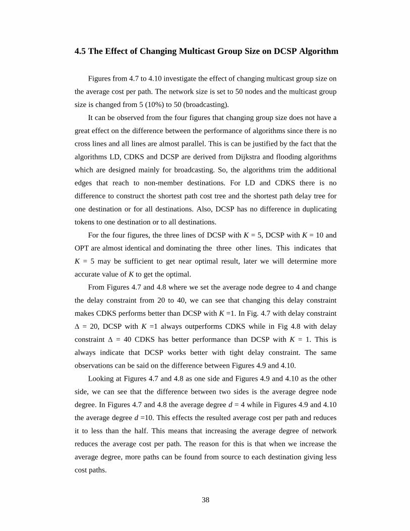
4.5 The Effect of Changing Multicast Group Size on DCSP Algor ithm
Figures from 4.7 to 4.10 investigate the effect of changing multicast group size on
the average cost per path. The network size is set to 50 nodes and the multicast group
size is changed from 5 (10%) to 50 (broadcasting).
It can be observed from the four figures that changing group size does not have a
great effect on the difference between the performance of algorithms since there is no
cross lines and all lines are almost parallel. This is can be justified by the fact that the
algorithms LD, CDKS and DCSP are derived from Dijkstra and flooding algorithms
which are designed mainly for broadcasting. So, the algorithms trim the additional
edges that reach to non-member destinations. For LD and CDKS there is no
difference to construct the shortest path cost tree and the shortest path delay tree for
one destination or for all destinations. Also, DCSP has no difference in duplicating
tokens to one destination or to all destinations.
For the four figures, the three lines of DCSP with K = 5, DCSP with K = 10 and
OPT are almost identical and dominating the three other lines. This indicates that
K = 5 may be sufficient to get near optimal result, later we will determine more
accurate value of K to get the optimal.
From Figures 4.7 and 4.8 where we set the average node degree to 4 and change
the delay constraint from 20 to 40, we can see that changing this delay constraint
makes CDKS performs better than DCSP with K =1. In Fig. 4.7 with delay constraint
� = 20, DCSP with K =1 always outperforms CDKS while in Fig 4.8 with delay
constraint � = 40 CDKS has better performance than DCSP with K = 1. This is
always indicate that DCSP works better with tight delay constraint. The same
observations can be said on the difference between Figures 4.9 and 4.10.
Looking at Figures 4.7 and 4.8 as one side and Figures 4.9 and 4.10 as the other
side, we can see that the difference between two sides is the average degree node
degree. In Figures 4.7 and 4.8 the average degree d = 4 while in Figures 4.9 and 4.10
the average degree d =10. This effects the resulted average cost per path and reduces
it to less than the half. This means that increasing the average degree of network
reduces the average cost per path. The reason for this is that when we increase the
average degree, more paths can be found from source to each destination giving less
cost paths.

39
250
270
290
310
330
350
370
390
410
430
450
5 10 15 20 25 30 35 40 45 50
Group Size
Avg
. Cos
t / P
ath
LD CDKS K=1K=5 K=10 OPT
Fig. 4.7. Effect of multicast group size with network size = 50, delay limit = 20,
average degree = 4
280
300
320
340
360
380
400
420
440
460
5 10 15 20 25 30 35 40 45 50
Group Size
Avg
. Cos
t / P
ath
LD CDKS K=1K=5 K=10 OPT
Fig. 4.8. Effect of multicast group size with network size = 50, delay limit = 40,
average degree = 4

40
125
130
135
140
145
150
155
160
165
170
175
180
185
5 10 15 20 25 30 35 40 45 50
Group Size
Avg
. Cos
t / P
ath
LD CDKS K=1K=5 K=10 OPT
Fig. 4.9. Effect of multicast group size with network size = 50, delay limit = 20, average
degree = 10
125
130
135
140
145
150
155
160
165
170
175
180
185
190
5 10 15 20 25 30 35 40 45 50
Group Size
Avg
. Cos
t / P
ath
LD CDKS K=1K=5 K=10 OPT
Fig. 4.10. Effect of multicast group size with network size = 50, delay limit = 40,
average degree = 10

41
4.6 The Effect of Changing Average Node degree on DCSP Algor ithm
Figures from 4.11 to 4.14 investigate the effect of changing average node degree
on the average cost per path. The network size is set to 50 nodes and the average node
degree is changed from 4 to 16.
For the four Figures, the three lines of DCSP with K = 10, DCSP with K = 20 and
OPT are almost identical and dominating the other three lines. This indicates that K =
10 may be sufficient to get near optimal result
It can be observed that the average cost per path for CDKS, DCSP and OPT is
decreased exponentially as the average node increases. First, there is a great
difference between network with average degree d = 4 and another one with d =6,
then, the difference in cost decreases and tends to be minor. This recommends that it
is enough to get a network with average degree d = 6.
In Figures 4.11 and 4.12, we set the delay constraint � = 20 and changing
multicast group size from 5 (10%) to 25 (50%). As indicated in the previous section,
changing multicast group size does not have a significant effect on the form of the
figure. The same can be applied to the Figures 4.13 and 4.14.
The difference between Figures 4.11 and 4.12 from one side and Figures 4.13 and
4.14 from the other side is the delay constrain � that changed from 20 to 40. In
Figures 4.11 and 4.12 DCSP with K = 1 always outperforms CDKS and the difference
between them increases with the increasing of average node degree. The situation is
fully reversed in Figures 4.13 and 4.14 where CDKS always outperforms DCSP with
K = 1 but the difference decreases with the increase of average node degree. This is
due to the relaxing of delay constraint, which is suitable for CDKS algorithm.
Figures 4.13 and 4.14 indicate that with the increase of the average node degree,
the performance of CDKS and DCSP with K = 1 always increases and it is almost get
near optimal value when average node degree d > 12. This means that with the large
average node degree, CDKS can find the optimal path from the large number of
possible paths. Also, K = 1 will be sufficient for DCSP to get the optimal results
which means that DCSP works better as the average node degree increased.

42
130
150
170
190
210
230
250
270
290
310
330
350
4 6 8 10 12 14 16Average Degree
Avg
. Cos
t / P
ath
LD CDKS K=1K=10 K=20 OPT
Fig. 4.11. Effect of average degree with network size = 50, multicast group = 5, delay
limit = 20
125
145
165
185
205
225
245
265
285
305
325
345
365
4 6 8 10 12 14 16Average Degree
Avg
. Cos
t / P
ath
LD CDKS K=1K=10 K=20 OPT
Fig. 4.12. Effect of average degree with network size = 50, multicast group = 25, delay
limit = 20

43
130
150
170
190
210
230
250
270
290
310
330
350
370
4 6 8 10 12 14 16Average Degree
Avg
. Cos
t / P
ath
LD CDKS K=1K=10 K=20 OPT
Fig. 4.13. Effect of average degree with network size = 50, multicast group = 5, delay
limit = 40
125
145
165
185
205
225
245
265
285
305
325
345
365
4 6 8 10 12 14 16Average Degree
Avg
. Cos
t / P
ath
LD CDKS K=1K=10 K=20 OPT
Fig. 4.14. Effect of average degree with network size = 50, multicast group = 25, delay
limit = 40

44
4.7 The Effect of Changing Delay Constraint on DCSP Algor ithm
Figures from 4.15 to 4.18 investigate the effect of relaxing delay constraint � on
the average cost per path. The network size is set to 50 nodes and the delay constraint
is changed from 10 to 60.
For the four Figures, we can observe that as the delay constraint increases, CDKS
is going toward OPT and after delay constraint � > 50, CDKS gives optimal results.
This can be justified by the fact that CDKS gives the optimal result at � = � where
the shortest path cost tree is the optimal result. So, for the large � the network almost
has no delay constraint.
In Figures 4.15 and 4.16, we set the average node degree d = 4 while changing
the multicast group from 5 to 25. The three lines of DCSP with K = 5, DCSP with
K = 10 and OPT are almost identical which means that for average degree d = 4,
K = 5 can give the optimal results. For the two Figures, DCSP with K = 1 is
dominating CDKS at small � (� < 22), as we relax the delay constraint, the
performance of DCSP with K = 1 decreases and the performance of CDKS increases.
When � > 22, CDKS outperforms DCSP with K = 1 and the difference is going to
increase with the increase of �.
Another point that is worth noting is the OPT line, we can see that the optimal
average cost per path is increasing while we relax the delay constraint, then the OPT
is going to be a horizontal line. This means that the performance of OPT is decreased
with less constraint. The justification of this is due to our simulation which run 3000
different graphs and take the average value over the graphs that have no failure. With
small delay constraint, the rate of failure is increased. As � increased the failure rate is
going to be a constant value giving the straight line. This is another point in favor to
DCSP over CDKS, that is in case of high failure rates DCSP still can get near optimal
values while CDKS can not afford it and it gives results that is near to the shortest
path delay tree which is obtained by LD algorithm.
In the four Figures, we can see that all lines are almost parallel except for CDKS,
this is because that LD and DCSP tend to minimize the delay while they work and this
is their first step to satisfy the delay constraint. On the other side, CDKS tends to
minimize the cost first then minimizing the delay.

45
300
320
340
360
380
400
420
440
460
10 20 30 40 50 60Delay Limit
Avg
. Cos
t / P
ath
LD CDKS K=1K=5 K=10 OPT
Fig. 4.15. Effect of delay limit with network size = 50, multicast group = 5, average
degree = 4
250
270
290
310
330
350
370
390
410
430
450
10 20 30 40 50 60Delay Limit
Avg
. Cos
t / P
ath
LD CDKS K=1K=5 K=10 OPT
Fig. 4.16. Effect of delay limit with network size = 50, multicast group = 25, average
degree = 4

46
130
135
140
145
150
155
160
165
170
175
180
185
190
10 20 30 40 50 60Delay Limit
Avg
. Cos
t / P
ath
LD CDKS K=1K=10 K=20 OPT
Fig. 4.17. Effect of delay limit with network size = 50, multicast group = 5, average
degree = 10
120
125
130
135
140
145
150
155
160
165
170
175
180
185
10 20 30 40 50 60Delay Limit
Avg
. Cos
t / P
ath
LD CDKS K=1K=10 K=20 OPT
Fig. 4.18. Effect of delay limit with network size = 50, multicast group = 25, average
degree = 10

47
If we compare between the two Figures 4.15 and 4.16 from one side and the two
Figures 4.17 and 4.18 as another side where we only change the average node degree
from 4 to 8, we can see the following.
1- The intersection point between the lines DCSP with K = 1 and CDKS is
increased from 22 to 34. This means that as the average node increases, the
performance of DCSP is going better and K = 1 can hold a value that is
better than CDKS for a larger delay constraint.
2- For the second set of Figures, K = 10 is sufficient to get the optimal result
while in the first, it was sufficient that K = 5 can get the optimal. This
indicates that with the increase of the average node degree we need larger
value of K.
3- For the second set of Figures, the OPT line tends to be a straight line as
� > 30, while in the first set, it was going to be a straight line at � > 50. This
means that the failure rate is decreased when the average node degree
increases. The justification of this is due to the increase of average node
degree, the possible paths increase so, the possibility of not finding a
suitable path is decreased.
4- The difference between the parallel lines of DCSP with K = 1 and OPT is
decreased in the second set, which again support the fact that DCSP gives
better results with the increase of average node degree.
5- As mentioned before, the increase of the average node degree results in the
decrease of the average cost path. The average cost per path for the second
set of Figures is almost less than half of the same value in the first set of
Figures.

48
4.8 The Effect of Changing Parameter K on DCSP Algor ithm
In all the previous figures, we always mention that K = 5 or K = 10 was sufficient
to get the optimal result. In this subsection, we determine more accurate value of K to
get the optimal solution under different values of the variables. To achieve this, we
only plot DCSP algorithm with the OPT algorithm and we change the value of
parameter K in DCSP algorithm.
The size of network is set to 50 nodes and we have three different variables to
change. Firstly, the multicast group size is given two values 5 and 25. Secondly, the
delay constraint is given two values 20 and 40. Thirdly, the average node degree is
given two values 4 and 10. Three variables each with two different values give eight
different Figures from 4.19 to 4.26.
In all Figures, DCSP is going toward the optimal exponentially with the increase
of K. This means that any small increase in K will yield to a significant improvement
in DCSP. Table 4.2 can summarize the results of the eight figures.
Table 4.2. The optimal value of K in network with 50 nodes.
Average Degree Delay L imit Multicast Group Optimal K
4 20 5 5
4 20 25 6
4 40 5 7
4 40 25 7
10 20 5 12
10 20 25 12
10 40 5 20
10 40 25 20
The eight Figures can be divided into three sets according to the value of optimal
K. In Figures from 4.19 to 4.22, we set the average node degree to 4 yielding the
optimal value of K around 6. In Figures 4.23 and 4.24, the average node degree is set

49
to 10 while the delay constraint � = 20 yielding an optimal K =12. The last set which
is Figures 4.25 and 4.26 where we set the average node degree = 10 and the delay
constraint � = 40 yields optimal K = 20. This indicates that the average node degree
has the most significant effect on K. As the average node degree increases, DCSP
needs a greater K to get the optimal results. Also, from the second and the third set,
we can see that relaxing the delay constraint results in a need for greater K. This is
because that relaxing delay limit means less killing of tokens in DCSP and hence the
system should keep track of greater number of tokens than if the delay constraint was
tight.
Fig. 4.19. Effect of K with network size = 50, multicast group = 5, delay limit = 20,
average degree = 4
300
303
306
309
312
315
318
321
324
327
330
333
1 2 3 4 5 6 7
K
Avg
. Cos
t / P
ath
DCSP Optimal
266
268
270
272
274
276
278
280
282
284
286
288
290
1 2 3 4 5 6 7 8
K
Avg
. Cos
t / P
ath
DCSP Optimal
Fig. 4.20. Effect of K with network size = 50, multicast group = 25, delay limit = 20,
average degree = 4

50
310
315
320
325
330
335
340
345
350
355
360
1 2 3 4 5 6 7 8 9 10
K
Avg
. Cos
t / P
ath
DCSP Optimal
Fig. 4.21. Effect of K with network size = 50, multicast group = 5, delay limit = 40,
average degree = 4
290
295
300
305
310
315
320
325
330
335
340
1 2 3 4 5 6 7 8 9 10
K
Avg
. Cos
t / P
ath
DCSP Optimal
Fig. 4.22. Effect of K with network size = 50, multicast group = 25, delay limit = 40,
average degree = 4
Fig. 4.23. Effect of K with network size = 50, multicast group = 5, delay limit = 20,
average degree = 10
139.3
139.5
139.7
139.9
140.1
140.3
140.5
140.7
2 4 6 8 10 12 14 16
K
Avg
. Cos
t / P
ath
DCSP Optimal

51
132.7
132.8
132.9
133
133.1
133.2
133.3
133.4
133.5
133.6
133.7
133.8
133.9
134
2 4 6 8 10 12 14 16 18
K
Avg
. Cos
t / P
ath
DCSP Optimal
Fig. 4.24. Effect of K with network size = 50, multicast group = 25, delay limit = 20,
average degree = 10
138.1
138.3
138.5
138.7
138.9
139.1
139.3
139.5
139.7
139.9
2 4 6 8 10 12 14 16 18 20
K
Avg
. Cos
t / P
ath
DCSP Optimal
Fig. 4.25. Effect of K with network size = 50, multicast group = 5, delay limit = 40,
average degree = 10
132.4
132.6
132.8
133
133.2
133.4
133.6
133.8
134
134.2
2 4 6 8 10 12 14 16 18 20
K
Avg
. Co
st /
Pat
h
DCSP Optimal
Fig. 4.26. Effect of K with network size = 50, multicast group = 25, delay limit = 40,
average degree = 10

52
4.9 Conclusion
Large number of simulation experiments have been done to compare DCSP
algorithm with previous algorithms, LD and CDKS, of the same problem and with the
OPT algorithm that always get the optimal results but in exponential time. Empirical
results show that DCSP always dominating other algorithms even with small K. Also,
in most cases DCSP approaches the optimal solution. In case of relaxed delay
constraint, CDKS dominate DCSP at K = 1. DCSP works better in case of tight delay
constraint and high average node degree. Simulation experiments have been used to
investigate a suitable number of the parameter K. In case of small value of K, the
complexity of DCSP is reduced from O(K2N2) to be O(N2).

53
Chapter 5
Proposed Shor test Path Algor ithm with
Delay and Delay Var iation Constraints
(DVCSP)
5.1 Introduction
In the last two chapters, the problem of multicast routing in real time networks is
investigated and formulated as shortest path routing under delay constraint. In this
chapter we add a delay variation constraint to the previous problem. The delay
variation constraint � is a bound on the variation among the delays along the
individual paths from source to each destination. This constraint is first mentioned
in [25] where the problem of finding a multicast tree that satisfy both delay and
delay variation constraint is proposed with the proof that it is an NP-Complete
problem. In [26] the cost factor is added, which results in a new problem for finding a
multicast tree with least cost and satisfying both delay and delay variation constraint.
This problem is also an NP-Complete as proved in [26].
The importance of delay variation arises from several applications. For example,
in a teleconference, it is important that the speaker be heard by all participants at the
same time, or the communication may lake the feeling of an interactive discussion.
When multicast messages are used to update multiple copies of replicated data item in
a distributed database system, minimizing the delay variation would minimize the

54
length of time that the database is in an inconsistent state. In a distributed game where
each player is connected to a game server and compete against other participants, it
will not be fair to delay one of the players more than the others by a certain value.
As proposed in [25], buffering can be used to control the delay variation but it
may not be practical. Buffering can be placed at the source node, switching nodes or
at the receivers. Buffering at the source would require the source to maintain
additional information about all destinations. This will make each message buffered
different amount of time for each destination and hence transmitted by the source
multiple times which violates the meaning of multicast routing. Buffering at the
switch nodes suffers from the same problems as buffering at source node. Buffering at
receiver nodes is more reasonable and it may have a good effect but it requires that all
destinations cooperate together. However, this may be accepted if all destinations
have the same task like the case of replicated database, but if the destinations are
competitors, it will be difficult to cooperate. Furthermore, the amount of buffering
needed is proportional to the maximum variation of end to end delays. Providing
bounds for delay variation will result in more efficient usage of buffering resources.
The rest of this chapter is organized as follows. In section 5.2, the problem of
shortest path under delay and delay variation constraints is formulated. A new
heuristic algorithm for this problem is proposed in section 5.3. The complexity
analysis of the proposed algorithm is introduced in section 5.4. Finally, the chapter is
concluded in section 5.5.
5.2 Problem formulation
Using the same notations and definitions listed in section 3.2 and defining � as
the delay variation constraint, the problem of shortest path multicast routing under
delay and delay variation constraints can be formulated as follows:
Given a directed, simple, connected weighted graph G(V,E), multicast group M⊆
V, a multicast source node s ∈ V , a delay constraint �, and a delay variation
constraint � where � < �. Find a subgraph G`(V`,E`) where ( {s} ∪ M ) ⊆ V` ⊆ V and
E` ⊆ E that has no cycles and no incoming edge in the source node s and all the leaves
should be members of M. G` should satisfy the following three conditions:
1- Minimum Cost(Path(s,v)) ∀ v ∈ M

55
2- Delay(Path(s,v)) < � ∀ v ∈ M
3- | Delay(Path(s,u)) - Delay(Path(s,v)) | < � ∀ u, v ∈ M
This problem is known to be NP-Complete[26]. So, any polynomial solution
tends to find a near optimal solution. If � > �, the problem is reduced to the delay
constrained shortest path problem discussed in chapter 3.
5.3 The Delay and Delay Var iation Constrained Shor test Path
Algor ithm (DVCSP)
DVCSP shown in Fig. 5.1 and described in appendix B.1, is a heuristic algorithm
to find a near optimal subgraph for the shortest path problem under delay and delay
variation constraints. DVCSP is a centralized algorithm where all the information
about the network topology is supposed to be kept at the source node. The algorithm
is divided into two separate phases. Phase I, the delay constraint phase, is responsible
for yielding a set of paths for each destination. These paths should satisfy the delay
constraint. If for some destinations, phase I is failed to find any path to that
destination, then the algorithm reports failure to satisfy the delay constraint. Phase II,
the delay variation constraint phase, collects all the paths from phase I and chooses
one path from each destination so that the delay variation constraint is satisfied. If
phase II is failed, then the algorithm reports failure to satisfy the delay variation
constraint and returns a subgraph with the minimum possible delay variation that is
can be resulted from DVCSP algorithm.
5.3.1 Phase I : The Delay Constraint Phase
This phase shown in Fig. 5.2 and described in appendix B.2, is similar to DCSP
algorithm described in chapter 3 where we use the same concept and structure of
token and token duplication. As in DCSP, phase I starts by an empty token at the
source node. The token is continuously duplicated to all neighbor nodes spanning all
possible paths in the network. To control the excessive number of tokens that results
from duplication, we limit the number of tokens that can be kept in any node at the

56
Report failure to
satisfy the delay
Start
Phase 1: Delay Constraint
For each destination node m
There is at least one
token in m
Next node m
Phase 2: Delay Var iation Constraint
The returned graph is the graph that
satisfies delay and delay variation
The returned graph form
Phase II satisfies delay
The returned graph is the one with the minimum possible value for delay variation
Y
N
Report failure to satisfy the delay variation constraint
End
N
Y
Fig. 5.1. The Flowchart of DVCSP algorithm

57
Start
Insert an empty token in source
No. of Tokens > 0
Fig. 5.2. The Flowchart for Phase I: Delay Constraint Phase
End
For each node u in V
For each Token T in node u
For each neighbor node v to node
Can_Duplicate
Duplicate_Token (T, u,
Next neighbor
Next token T
Next node u
Delete the token T
Y
Y
N
N
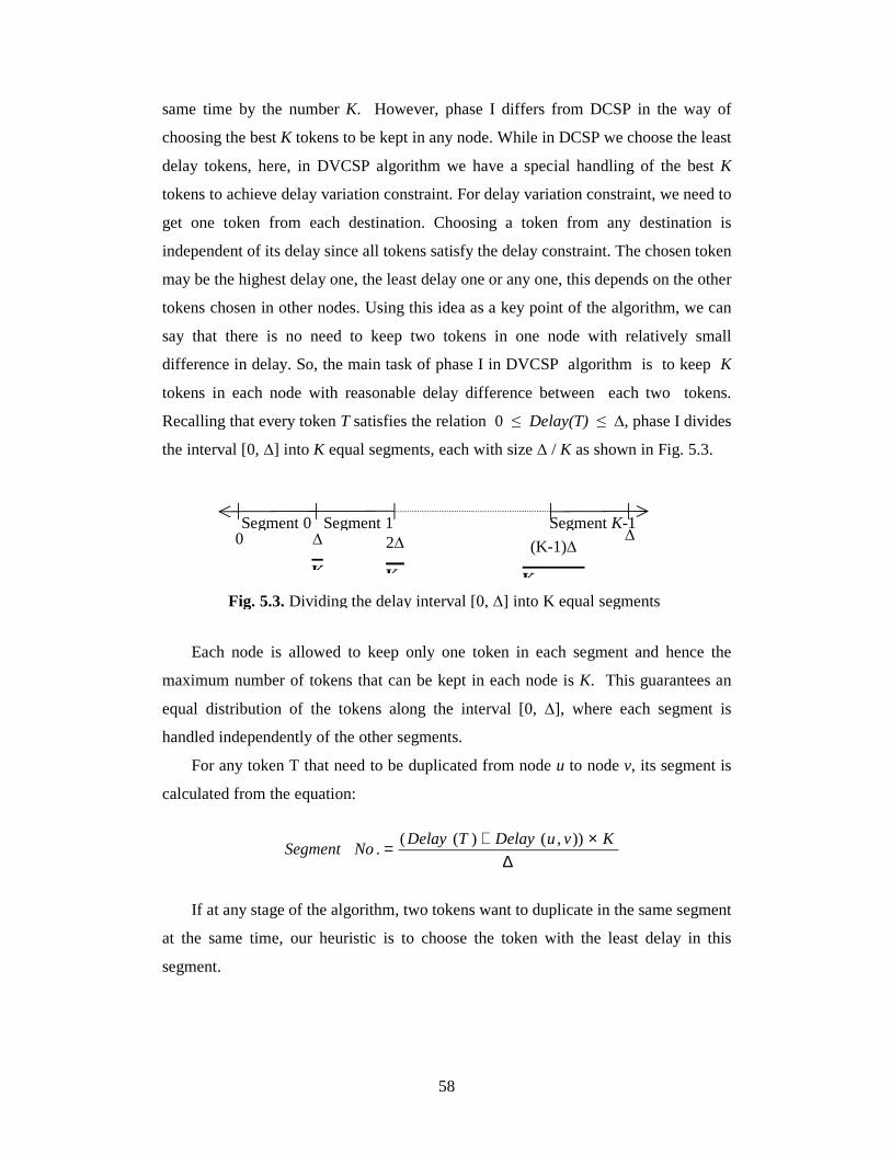
58
same time by the number K. However, phase I differs from DCSP in the way of
choosing the best K tokens to be kept in any node. While in DCSP we choose the least
delay tokens, here, in DVCSP algorithm we have a special handling of the best K
tokens to achieve delay variation constraint. For delay variation constraint, we need to
get one token from each destination. Choosing a token from any destination is
independent of its delay since all tokens satisfy the delay constraint. The chosen token
may be the highest delay one, the least delay one or any one, this depends on the other
tokens chosen in other nodes. Using this idea as a key point of the algorithm, we can
say that there is no need to keep two tokens in one node with relatively small
difference in delay. So, the main task of phase I in DVCSP algorithm is to keep K
tokens in each node with reasonable delay difference between each two tokens.
Recalling that every token T satisfies the relation 0 � Delay(T) � �, phase I divides
the interval [0, �] into K equal segments, each with size � / K as shown in Fig. 5.3.
Each node is allowed to keep only one token in each segment and hence the
maximum number of tokens that can be kept in each node is K. This guarantees an
equal distribution of the tokens along the interval [0, �], where each segment is
handled independently of the other segments.
For any token T that need to be duplicated from node u to node v, its segment is
calculated from the equation:
If at any stage of the algorithm, two tokens want to duplicate in the same segment
at the same time, our heuristic is to choose the token with the least delay in this
segment.
0 Segment 0
�
K
2�
K
Segment 1 Segment K-1 (K-1)�
K
�
Fig. 5.3. Dividing the delay interval [0, �] into K equal segments
∆×+= KvuDelayTDelay
NoSegment)),()((
.

59
So, compared to DCSP algorithm, in DVCSP there is only three constraints that
can prevent token duplication from node u to node v.
1. The sum of token delay and Delay(u,v) will exceed the delay constraint �.
2. The token T visited the node v before.
3. There is another token T1 in the same segment that T wants to duplicate in and
Delay(T1) < Delay(T).
The first two constraints are the same as the first two constraints in DCSP
algorithm and they mean that the duplicated token should not exceed the delay limit
and should not make a loop. The third constraint is the heuristic constraint specialized
for delay variation constraint.
In DCSP algorithm we keep at each destination one token only called the winner
token. However, in DVCSP, each destination node u ∈ M keeps track with at most 3K
tokens representing three tokens in each segment. For each segment the destination
keeps track with the least delay, least cost and the highest delay tokens passed through
this segment. The least delay token is used to guarantee finding a solution for the
delay constraint. The highest delay token is used to give an upper bound for the delay
in this node. The least cost token is used as a moderation between the least delay and
the highest delay tokens, it is also used to minimize the cost of the resulted graph.
These tokens are used by phase II to select only one of them. Phase I is finished when
all the tokens in the system are either killed or kept in the destination nodes.
Phase I has two main subroutines, the function Can_Duplicate and the procedure
Duplicate_Token
5.3.1.1 The function : Can_Duplicate (Token T, Node u, Node v)
The function Can_Duplicate shown in Fig. 5.4 and described in appendix B.3,
takes three inputs:
4- Token T
5- Node u that currently holds the token T
6- Node v that the token T needs to be duplicated in.

60
Start
Delay(T) + Delay(u,v) >
�
Fig. 5.4. The Flowchart for the function Can_Duplicate(T, u, v)
Return True
T visited node v before
Node v has token T1 in
Segment_No
Delay(T1) < Delay(T)
Return False
Y
Y
Y
Y
N
N
N
N
Segment_No =(Delay(T) * K) / �
Delete token T1

61
The function applies the three constraints discussed in the previous section and
returns True if the token T can be duplicated from node u to node v, otherwise, the
function returns False.
5.3.1.2 The Procedure : Duplicate_Token (Token T, Node u, Node v, Group M)
The procedure Duplicate_Token shown in Fig. 5.5 and described code in
appendix B.4, is executed only if the function Can_Duplicate(T,u,v) returns true. The
procedure has four inputs:
1- Token T
2- Node u that currently holds the token T
3- Node v that the token T needs to be duplicated in.
4- Multicast Group M
Duplicate_Token is responsible of updating the cost and the delay of the
duplicated token T by adding Cost(u,v) and Delay(u,v) to Cost(T) and Delay(T)
respectively. It also puts the timestamp of node v in token T and increases the number
of tokens in the system by one for the new generated token.
If the node v is in multicast group M, then the procedure calculates the segment
number that token T duplicated in, and updates the least delay, the highest delay and
the least cost tokens in this segment.
5.3.2 Phase I I : The Delay Var iation Constraint Phase
Phase II shown in Fig. 5.6 and described in appendix B.5, is responsible of
satisfying the delay variation constraint. This phase is started by collecting all the
tokens from the destinations that left from phase I in one array called merged_array.
Since, at most each destination can have 3K tokens, so, the total number of tokens in
merged_array will be at most 3mK tokens. The merged_array contains two fields, the
token field that contains the token data, and the destination field that contains the
destination that we get this token from. This array is then sorted in ascending order
according to the delay field of each token.
Two pointers are moved through the sorted array, start_pointer and end_pointer
where always start_pointer < end_pointer and Delay(Te) – Delay(Ts) < � where Ts is

62
Start
Node v puts a timestamp on
No. of tokens = No. of tokens +1
Cost(T) = Cost(T) + Cost(u,v)
Delay(T) = Delay(T) + Delay(u,v)
End
Fig. 5.5. The Flowchart for the procedure
Segment_No =((Delay(T)+Delay(u,v)) *
Delay(T) <
Least_delay[ Segment_No
Least_delay[ Segment_No] =Delay(T)
N
Y
Delay(T) >
Highest_delay[ Segment_
Highest_delay[ Segment_No]
N
Y
Cost(T) <
Least_cost[ Segment_No]
Least_cost[ Segment_No] =Cost(T)
N
Y
v ∈ M
Y
N

63
Start
Collect all tokens from destination
nodes into one array called
Sort merged_array in ascending order
according to the delay of each token in
For start_pointer = 0 to the last element in
end_pointer =start_pointer
Ts = The token at the start_pointer
T = The token at the end_pointer
Set all elements in cost_window
array to ∞
Delay(Te) - Delay(Ts) < δ
cost_window[ D] = ∞
total_cost=total_cost+Cost(
T )
total_cost=total_cost-
cost_window[D] <
N
N
Y
end_pointer=
N
Y
Y
cost_window contains ∞
N
total_cost > best_cost Y
best_cost = total_cost
best_window = cost_window
Next
The resulted subgraph is
the graph consisting of all
End
Fig. 5.6. The Flowchart for Phase II, Delay Variation Constraint Phase
N
Y
best_window contains ∞ Y
N Report Failure in delay
variation

64
the token that the start_pointer points to and Te is the token that the end_pointer
points to. The idea behind this phase is to let the difference between end_pointer and
start_pointer as large as possible. By looking at the tokens in the interval
[start_pointer, end_pointer], if there is at least one token represents each destination
in this interval, then we choose the least cost token for each destination and consider it
as a feasible solution, otherwise, we consider that this interval has no solution in it.
Then we move the start_pointer by one step and updates the end_pointer to make
their difference as large as possible. This yields to a new interval that we can check it
again. From all feasible solutions we get, we choose the solution with the least cost.
The algorithm is continued till the start_pointer reaches the end of the merged_array.
If no feasible solution is found in all the checked intervals, then phase II reports
failure to satisfy the delay variation constraint and invokes the procedure
Get_Minimum_Variation that returns subgraph with minimum possible delay
variation.
To implement this phase, we have an array called cost_window that contains the
least cost token of each destination that is found in the interval
[start_pointer,end_pointer]. At the beginning of each interval, all the elements in
cost_window are initialized to �. For each interval we have a different cost_window,
so, the best_window array is used to keep track with the best cost_window array
examined so far in terms of its total cost. The final value of best_window array
contains the tokens that participate in the resulted subgraph. The variable total_cost is
used to keep track of the total cost that cost_window array has, and it is initialized by
zero. The variable best_cost is used to keep track of the total cost that best_window
array has.
The algorithm starts by setting the start_pointer and end_pointer to the first
element in merged_array. The end_pointer is advanced step by step if it satisfies the
condition Delay(Te) – Delay(Ts) < �. At each step of advancing the end_pointer we
check Te and look for the destination D that we get this token from. If the place of
destination D in the cost_window array contains �, this means that this is the first
token we get in this interval that represent the destination D, so we increment the
total_cost by Cost(Te) and set the place of D in cost_window array to the value of
Cost(Te). On the other hand, if cost_window has some value in the D place, this means
that we get another token that represents this destination, so, we will compare

65
Cost(Te) with cost_window[ D] and choose the one with least cost and update the
total_cost variable.
When the interval is completed, we check whether it has any element that
contains � or not and if true this means that this interval has no feasible solution,
otherwise, the cost_window contains a feasible solution. All feasible solutions are
investigated yielding to the best one in best_window array.
5.3.2.1 The Procedure : Get_Minimum_Variation (Group M)
This procedure shown in Fig. 5.7 and described in appendix B.6, is executed only
when phase II fails to satisfy the delay variation constraint. It returns a subgraph with
the minimum possible value of delay variation that can be extracted from DVCSP
algorithm. This procedure has a significant effect in that it can give an indicator to
how can DVCSP satisfy the delay variation constraint. Also, the result from this
procedure could be used in negotiations between the user requirements and the
capability of the routing algorithm.
The procedure uses the same array, merged_array, that is collected at the start of
phase II. A single pointer called start_pointer is moved along the array. An array
called delay_window is used to keep track of a token from each destination. All
elements in delay_window is initialized by �. The start_pointer is initialized at the
first element of merged_array and then it moves only forward to the last element of
the array. The token that start_pointer points to is placed in its place in delay_window
according to the destination it comes from. No processing is done in delay_window
until all its places is filled with values rather than �. When it is happened we consider
it as the first window to process and calculate the difference between maximum and
minimum values inside delay_window which is called the variation in delay_window.
With every movement of start_pointer, we have another values for delay_window
with another value of its variation. From all the windows we investigate, we choose
the one with best variation. This is considered to be the best delay variation the
DVCSP can get from the network. The procedure is finished when start_pointer
reaches the last element in merged_array.

66
Start
For start_pointer = 0 to the last element in
Ts = The token at the start_pointer
D = The destination that we got Te
Set all elements in delay_window
array to ∞
delay_window contains ∞
N
Y
N
Y
delay_window[ D] =
Var = The difference between maximum
and minimum values of
Var > best_delay
best_delay = Var
best_window =
Next start_pointer
The resulted graph conisted from
the tokens that is in best_window
End
Fig. 5.7. The Flowchart for the procedure Get_Minimum_Var iation (M)

67
5.4 Analysis and Complexity of DVCSP Algor ithm
Lemma 5.1
DVCSP algorithm always finds a solution for the delay constrained problem if
one exists and if DVCSP fails to find a feasible solution for the delay constraint,
then there is no other algorithm can find it.
Proof
Recalling the proof of lemma 3.1, it will be sufficient to prove that DVCSP
will perform in its worst case and in case of K = 1 as the shortest path delay
algorithm. In case of K = 1, we have only one segment at each node. Any
collision at this node will result in selecting the node with the least delay, so we
guarantee that the least delay token continues its trip and results in the least
delay path. If K > 1, each node will have K segments and since we deal with
each segment independently and keep the least delay token in each one, so the
least delay token in the first segment that lies in the interval [0, � / K] is the
least delay token that can reach this node. If for any destination u ∈ M, the least
delay token does not satisfy the delay constraint, then this means that there is no
feasible solution and no other algorithm can find a solution since the shortest
path delay is optimal with respect to the delay constraint.
Lemma 5.2
Phase II in DVCSP algorithm finds an optimal solution for delay variation
constraint from the data returned from Phase I.
Proof
In phase II, we collect all the tokens from the destinations in one array. The
maximum number of tokens is 3mk. Since, we initialize the start_pointer and
end_pointer at the first element of the array, then we move the end_pointer step
by step to get the interval [start_pointer, end_pointer]. After examining this
interval, we move the start_pointer one step, and initialize the end_pointer to be
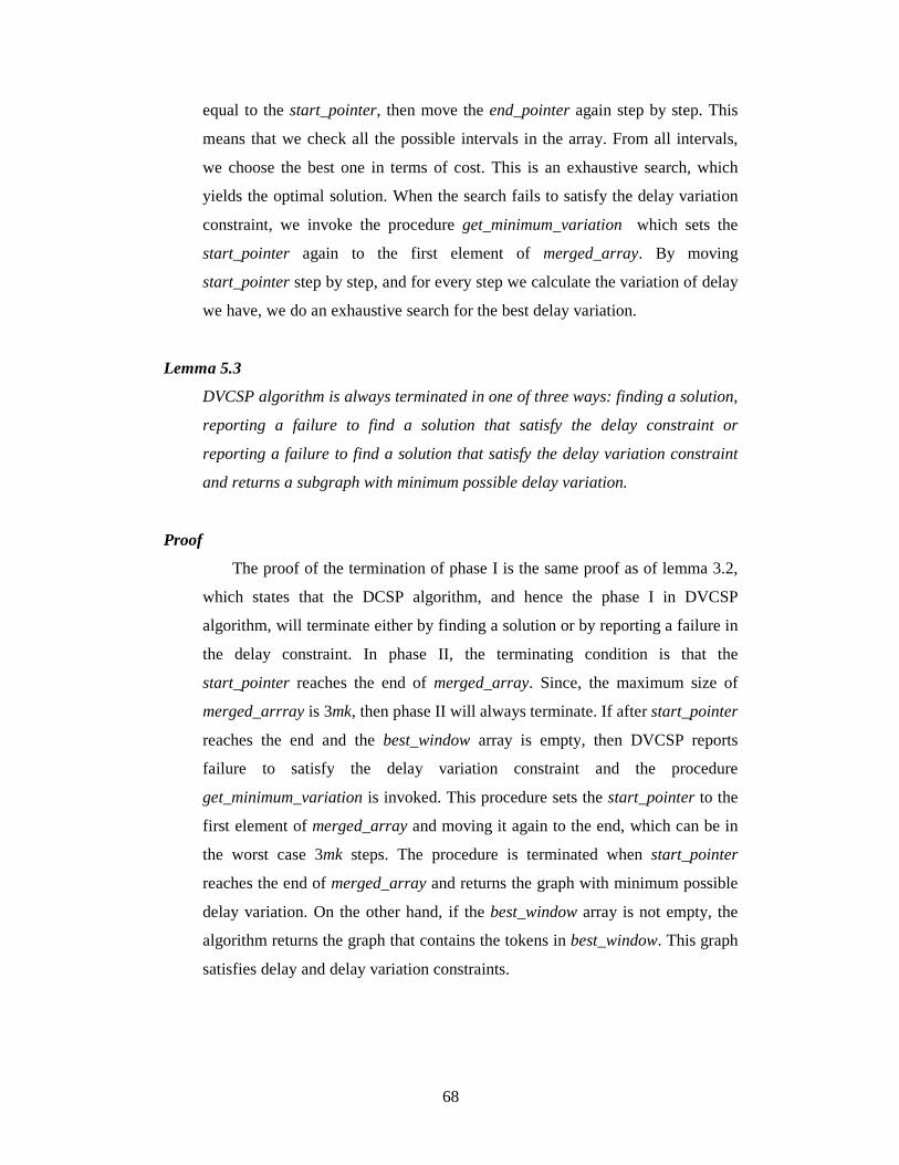
68
equal to the start_pointer, then move the end_pointer again step by step. This
means that we check all the possible intervals in the array. From all intervals,
we choose the best one in terms of cost. This is an exhaustive search, which
yields the optimal solution. When the search fails to satisfy the delay variation
constraint, we invoke the procedure get_minimum_variation which sets the
start_pointer again to the first element of merged_array. By moving
start_pointer step by step, and for every step we calculate the variation of delay
we have, we do an exhaustive search for the best delay variation.
Lemma 5.3
DVCSP algorithm is always terminated in one of three ways: finding a solution,
reporting a failure to find a solution that satisfy the delay constraint or
reporting a failure to find a solution that satisfy the delay variation constraint
and returns a subgraph with minimum possible delay variation.
Proof
The proof of the termination of phase I is the same proof as of lemma 3.2,
which states that the DCSP algorithm, and hence the phase I in DVCSP
algorithm, will terminate either by finding a solution or by reporting a failure in
the delay constraint. In phase II, the terminating condition is that the
start_pointer reaches the end of merged_array. Since, the maximum size of
merged_arrray is 3mk, then phase II will always terminate. If after start_pointer
reaches the end and the best_window array is empty, then DVCSP reports
failure to satisfy the delay variation constraint and the procedure
get_minimum_variation is invoked. This procedure sets the start_pointer to the
first element of merged_array and moving it again to the end, which can be in
the worst case 3mk steps. The procedure is terminated when start_pointer
reaches the end of merged_array and returns the graph with minimum possible
delay variation. On the other hand, if the best_window array is not empty, the
algorithm returns the graph that contains the tokens in best_window. This graph
satisfies delay and delay variation constraints.

69
Lemma 5.4
The worst case complexity of DVCSP is O(K2M2) if KM2 > N2 and O(KN2) if
KM2 < N2, where K is an integer value ranged from 1 to N, M = |M| the number
of nodes in the multicast group and N = |V| the number of nodes in the network.
Proof
The proof of complexity of phase I in DVCSP algorithm is similar to the
proof of lemma 3.3. Just one difference that the function can_duplicate in DCSP
algorithm is O(K) while in DVCSP algorithm it is O(1). So, phase I in DVCSP
algorithm has the worst case complexity of O(KN2). This is the same as DCSP
but after removing K for the can_duplicate function. In phase II, the maximum
number of elements in the merged_array is 3mK elements. Sorting this array
can be done in O(MK log MK ). Moving start_pointer from the first element of
the array to the last element is O(MK). At each time the start_pointer is moved,
the end_pointer will be updated. The worst case can happen when the delay
variation constraint is so large that the end_pointer every time will be moved
from the start_pointer to the end of the array. This will make the movement of
end_pointer is also O(MK). Moving the end_pointer inside the start_pointer
resulting in making phase II O(M2K2). In case of failure to satisfy delay
variation constraint, phase II calls the procedure get_minimum_variation. This
procedure move the start_pointer from the first element in merged_array to the
last element, so, the worst case complexity of moving start_pointer is O(MK).
At every move, we calculate the maximum and minimum value of
delay_window to get the maximum variation of this array. Since delay_window
contains only M elements, so, the worst case complexity of this procedure is
O(M2K). So, phase II contains three sequential complexities which are
O(MK log MK ), O(M2K2) and O(M2K). Since phase I and phase II are executed
sequentially, then DVCSP, in its worst case complexity, will be executed in
O(KN2 + MK log MK + M2K2 + M2K) steps. For the four terms that constitute
the complexity order, the term M2K2 will be dominant if KM2 > N2 which makes
DVCSP of O(M2K2). If KM2 < N2 , the term KN2 will dominate the other three
terms and the total complexity of DVCSP will be O(KN2).

70
5.5 Conclusion
In this chapter, we considered the problem of multicast routing with two QoS
parameters, which are delay and delay variation. The problem is formulated as shortest
path problem under delay and delay variation constraints. This problem is known to be
NP-Complete. A polynomial time heuristic algorithm, called DVCSP, for this problem
is proposed. The proposed algorithm is discussed in depth aided with flowcharts for
the most important used subroutines. The pseudo codes of the algorithm are listed in
appendix B. The algorithm has running time complexity of O(K2M2) if KM2 > N2 and
O(KN2) if KM2 < N2 , where K is an integer value ranged from 1 to N, M = |M| the
number of nodes in the multicast group and N = |V| the number of nodes in the
network.

71
Chapter 6
Per formance Analysis of the Proposed
DVCSP Algor ithm
6.1 Introduction
In this chapter, we do a comprehensive analysis of the proposed DVCSP
algorithm and compare it with other algorithms. We use the same random graph
generator described in section 4.2. The simulated algorithms are presented in section
6.2. In section 6.3, we present the performance factors that is used to evaluate the
different algorithms. The effect of relaxing the delay variation constraint is
investigated in section 6.4. In section 6.5, we examine the effect of changing the
multicast group size on the different algorithms. The effect of increasing the number
of nodes in the network is investigated in section 6.6. Finally, the chapter is concluded
in section 6.7.
6.2 Simulated Algor ithms
The random graph generator described in section 4.2 is used to simulate and
compare the following:
1- The shortest path delay tree (LD) obtained by applying Dijkstra algorithm [3].
2- CDKS algorithm [8], designed for the delay constrained shortest path tree. It
first constructs the shortest path cost tree. Then, it looks for every destination
and tests it according to the delay constraint �. If the destination satisfies �,

72
then the shortest path cost for this destination will be in the resulted tree,
otherwise, it replaces the path for this destination from the shortest path delay
tree.
4- The DCSP algorithm that is proposed in chapter 3 for the delay constrained
shortest path problem. We set the value of parameter K to 10, since it is almost
the best value for this algorithm as can be deduced from the simulation
experiments in chapter 4.
5- The proposed DVCSP algorithm that is designed for the delay and delay
variation constrained shortest path problem. To investigate the effect of
parameter K on DVCSP algorithm, we choose three values of K that is 1, 10, 20
to be compared in each simulation experiment.
6.3 Performance Factors
For all the simulated algorithms, we consider two performance factors, the
failure rate and the average cost per path of the resulted tree.
6.3.1 Failure Rate
Any algorithm can fail to find a suitable tree by not satisfying either the delay
constraint or the delay variation constraint. Recalling the proof of lemma 3.1 and
lemma 5.1, and from the definition of LD and CDKS algorithms, all the algorithms
will find a delay constrained tree if one exists. So, all simulated algorithms have the
same failure rate to find a delay constrained tree. Hence, we will not use the failure in
the delay constraint as a performance factor. On the other side, the failure of finding a
tree that satisfies the delay variation constraint is different for all algorithms and gives
an indication of how suitable these algorithms to the delay variation constraint. So, we
define the failure rate as the rate that the algorithm failed to find a tree that satisfies
the delay variation constraint.
6.3.2 Average Cost per Path
The second performance factor we measure is the average cost per path of the
resulted tree. For the algorithms LD, CDKS and DCSP that is designed mainly for the
delay constrained shortest path tree problem, we calculate the cost whether the

73
algorithm failed to satisfy the delay variation constraint or not. For DVCSP algorithm,
when the failure happened, we calculate the cost of the tree with minimum possible
delay variation.
6.4 The Effect of Changing Delay Var iation on DVCSP Algor ithm
6.4.1 Failure Rate
Figures 6.1, 6.2 and 6.3 investigate the effect of changing delay variation
constraint on the failure rate. For the three figures, we set the number of nodes in the
network N = 50 and the delay constraint � = 20, while changing the delay variation
constraint � from 0 to 20. Setting the delay variation constraint to 0 means that all the
destinations should get the data at the same time while setting � = 20, the same value
as �, cancels the effect of delay variation constraint.
In Fig. 6.1, we set the average node degree d = 4 and the multicast group size M
= 5. It can be observed that DVCSP algorithm dominates all other algorithms even
with K =1. The two lines of DVCSP with K = 10 and K = 20 are almost identical
except when � =0, this indicates that K = 10 is sufficient to get reasonable results for
DVCSP algorithm. With tight delay variation constraint, the performance of LD,
CDKS and DCSP is very bad with DCSP the worst. LD algorithm is always better
than CDKS and DCSP, this is can be deduced from the fact that LD tends to minimize
the delay and hence all the destination have the lowest possible delay. The failure rate
of all algorithms is zero at � = � = 20 this is because the problem is reduced to be
shortest path problem under delay constraint
Fig. 6.2 differs from Fig. 6.1 in the size of multicast group M which is set to 25
instead of 5. The increase in multicast group size raises the difficulty of satisfying the
delay variation constraint. CDKS and DCSP algorithms have a very bad response for
this increase where they give 100% failure at � < 12, also LD gives 100% failure at
� < 10. DVCSP still dominates the other algorithms and the two lines of DVCSP at
K = 10 and K = 20 are almost identical except for � = 0.
Fig. 6.3 differs from Fig. 6.1 in the average node degree d where we set it to 10
instead of 4. Increasing the average degree increases the number of available paths,
which results in decreasing the failure rate. DVCSP with K = 10 and K = 20 almost
have zero failure rate for all delay variations even when � = 0. DVCSP with K = 1

74
gives zero failure rate at � > 8. The performance of LD, CDKS and DCSP is enhanced
but it still gives 100% failure at small �.
0
10
20
30
40
50
60
70
80
90
100
0 2 4 6 8 10 12 14 16 18 20
Delay Variation
Perc
enta
ge o
f fa
ilure
rat
e
LD CDKS DCSPK=1 K=10 K=20
Fig. 6.1. Effect of delay variation constraint on failure rate with network size = 50,
delay constraint = 20, multicast group = 5, average node degree = 4.
0
10
20
30
40
50
60
70
80
90
100
0 2 4 6 8 10 12 14 16 18 20
Delay Variation
Per
cent
age
of f
ailu
re r
ate
LDCDKSDCSPK=1K=10K=20
Fig. 6.2. Effect of delay variation constraint on failure rate with network size = 50,
delay constraint = 20, multicast group = 25, average node degree = 4.

75
6.4.2 Average Cost per Path
Figures 6.4, 6.5 and 6.6 investigate the effect of changing delay variation
constraint on average cost per path. For the three figures, we set the number of nodes
in the network N = 50 and the delay constraint � = 20, while changing the delay
variation constraint � from 0 to 20.
For the three figures, it can be observed that the three lines of LD, CDKS and
DCSP algorithm are constant values. This means that the cost of the resulted tree is
not dependent on the delay variation constraint. This is can be deduced from the fact
that the three algorithms are mainly developed to the problem of shortest path tree
under delay constraint. So, they do not give any attention to the delay variation
constraint. Always the performance of DCSP is better than CDKS which is better than
LD. This agrees with the results of simulation experiments done in chapter 4.
In Fig. 6.4, we set the average node degree d = 4 and the multicast group size M
= 5. DVCSP with K = 1 gives very high cost that is not comparable to any other
algorithm when � < 8, then it approaches the same performance of CDKS at � > 16.
DVCSP with K = 10 and K = 20 always have a small difference in cost, and this
indicates that K = 10 is sufficient for DVCSP. At � < 6, DVCSP with K =10 and
K = 20 results in a very high cost.
Fig. 6.3. Effect of delay variation constraint on failure rate with network size = 50,
delay constraint = 20, multicast group = 5, average node degree = 10.
0
10
20
30
40
50
60
70
80
90
100
0 2 4 6 8 10 12 14 16 18 20
Delay Variation
Perc
enta
ge o
f fa
ilure
rat
e
LD CDKS DCSPK=1 K=10 K=20

76
300
330
360
390
420
450
480
510
540
0 2 4 6 8 10 12 14 16 18 20Delay Variation
Avg
. Cos
t/Pat
h
LD CDKS DCSPK=1 K=10 K=20
Fig. 6.4. Effect of delay variation constraint on average cost per path with network size = 50,
delay constraint = 20, multicast group = 5, average node degree = 4.
280
320
360
400
440
480
520
560
600
0 2 4 6 8 10 12 14 16 18 20Delay Variation
Avg
. Cos
t/Pat
h
LD CDKS DCSPK=1 K=10 K=20
Fig. 6.5. Effect of delay variation constraint on average cost per path with network size = 50,
delay constraint = 20, multicast group = 25, average node degree = 4.

77
This cost is considered to be paid for the added constraint. Recalling that at
small �, it was very difficult to obtain a solution for the other algorithms, so, finding a
solution at small � should be with a very high cost. The performance of DVCSP with
K = 20 is enhanced at relaxing the delay variation constraints and it dominates CDKS
at � > 10, then it approaches DCSP but it never overcomes it. It is always that DVCSP
never dominate DCSP because DVCSP uses DCSP with an additional constraint
which results in an additional cost. Comparing DVCSP with CDKS when � > 10
yielding that, although DVCSP has an additional constraint, it also gives better cost.
In Fig. 6.5, we increase the multicast group size M to 25, this gives almost the
same graph of Fig. 6.4 with the same analysis. This is indicates that changing
multicast group does not have a significant effect on the average cost per path. This is
because all the compared algorithms deal with multicast as a special case of
broadcasting, so, it does not matter how large is the size of the multicast group.
130
140
150
160
170
180
190
200
0 2 4 6 8 10 12 14 16 18 20Delay Variation
Avg
. Cos
t/Pat
h
LD CDKS DCSPK=1 K=10 K=20
Fig. 6.6. Effect of delay variation constraint on average cost per path with network size = 50,
delay constraint = 20, multicast group = 5, average node degree = 10.

78
Fig. 6.6 differs from Fig. 6.4 in the average node degree d which is set to 10
instead of 4. The performance of DVCSP is enhanced with the increase of average
node degree. The difference between DVCSP with K = 20 and DCSP is decreased.
Also, DVCSP with K = 1 dominates CDKS when � > 14. For all algorithms, the
average cost per path is decreased to half of its value in Fig. 6.4. This is because that
increasing average degree results in more available paths which results in available
cheaper paths.
6.5 The Effect of Changing Multicast Group Size on DVCSP Algor ithm
6.5.1 Failure Rate
The effect of changing multicast group size on the failure rate is investigated in
the Figures 6.7, 6.8 and 6.9. For the three figures, we set the network size N = 50,
delay constraint � = 20 while changing the multicast group size from 5 to 45.
Increasing the size of multicast group makes the problem of delay variation
constraint more difficult, since finding suitable values for delay in 45 nodes is more
difficult than finding it for 5 nodes. For all graphs, the two lines of DVCSP with
K = 10 and K = 20 almost identical for all values of M. So, K = 10 is sufficient for
DVCSP to get its best performance.
In Fig. 6.7, we set the average node degree d = 4 and we force a tight delay
variation constraint � = 5. It can be observed that for tight delay variation, LD, CDKS
and DCSP algorithms does not work at all since they give 100% failure rate at
M > 10. This indicates that these algorithms are not suitable for the delay variation
constrained problem.
On the other side, DVCSP with K = 10 gives relatively good results and its
failure rate increased slightly with the increase of multicast group. This indicates that
DVCSP is working well even in tight delay constraint and in large multicast group
size. DVCSP with K = 1 has a higher failure rate than K = 10 and K = 20 by
almost a constant difference 15% in the different sizes of multicast group.
In Fig. 6.8, we still keep the tight delay variation constraint while increasing the
average node degree d to 10 instead of 4. This is to increase the number of available
paths and to decrease the failure rate of all algorithms. However, CDKS and DCSP
still effected by the tight delay variation, so, they have no performance enhancement

79
0
10
20
30
40
50
60
70
80
90
100
5 10 15 20 25 30 35 40 45
Group Size
Perc
enta
ge o
f fa
ilur
e ra
te
LD CDKS DCSPK=1 K=10 K=20
Fig. 6.7. Effect of multicast group size on failure rate with network size = 50, delay
constraint = 20, delay variation constraint = 5, average node degree = 4.
0
10
20
30
40
50
60
70
80
90
100
5 10 15 20 25 30 35 40 45
Group Size
Perc
enta
ge o
f fa
ilur
e ra
te
LD CDKS DCSPK=1 K=10 K=20
Fig. 6.8. Effect of multicast group size on failure rate with network size = 50, delay
constraint = 20, delay variation constraint = 5, average node degree = 10.

80
for the increase of the average node degree where they have 100% failure rate when
M > 10. Also, LD has a failure rate of 100% when M > 15. On the other hand,
DVCSP performs well with the increase of the average node degree even with the
tight delay variation. DVCSP with K = 10 and K = 20 have almost zero failure for all
different multicast group sizes. This indicates that DVCSP works better for networks
with high average node degree.
Fig. 6.9 differs from Fig. 6.7 in that we relax the delay variation constraint � to
be 15 instead of 5 while keeping the average node degree d = 4. The effect of relaxing
the delay variation constraint is significant to all algorithms. CDKS and DCSP
perform well in small multicast group but they still cannot stand out with large
multicast group size. LD always has a failure rate below 50%, recalling that it was
always 100% in Fig. 6.7 yielding that LD has the best response for relaxing delay
variation. DVCSP with K = 10 and K = 20 have a good performance and they always
results in a failure rate that is below 5%. The difference between DVCSP with K = 1
and the other values of K is decreased. This indicates that for large delay variation
constraint we can reduce the value of K.
0
10
20
30
40
50
60
70
80
90
100
5 10 15 20 25 30 35 40 45
Group Size
Perc
enta
ge o
f fa
ilur
e ra
te
LD CDKS DCSPK=1 K=10 K=20
Fig. 6.9. Effect of multicast group size on failure rate with network size = 50, delay
constraint = 20, delay variation constraint = 15, average node degree = 4.

81
6.5.2 Average Cost per Path
Figures 6.10, 6.11 and 6.12 investigate the effect of changing multicast group
size M on the average cost per path for the resulted tree. For the three figures, we set
the network size N = 50, the delay constraint � = 20 while changing the multicast
group size from 5 to 45.
In Fig. 6.10, we set the delay variation constraint � = 5 and the average node
degree d = 4. DCSP always dominate the other algorithms, this is the result of high
failure rate. DVCSP with K = 10 and K = 20 yield a cost which is worse than CDKS
and better than LD. The additional cost that DVCSP suffers from is due to its low
failure rate. We should pay an additional cost to satisfy an additional constraint.
DVCSP with K = 1 is not practical at all since it gives relatively high cost.
In Fig. 6.11, we increase the average node degree d to 10 while keeping the tight
delay variation constraint. Comparing between DVCSP and CDKS, It is observed that
DVCSP with K = 10 and K = 20 give better cost and better failure rate, which means
that in all factors DVCSP dominates CDKS in case of large average node degree.
DCSP still get the best result in terms of cost. This assists the results obtained from
chapter 4, which states that DCSP with K = 10 always gives near optimal results
under all circumstances. DVCSP with K = 1 still gives a very high cost which makes
it not practical. This is because that DVCSP with K = 1 trying to solve the problem of
delay variation constraint with few resources which results in more cost. Also, the
increase of average node degree results in less cost for all algorithms.
Fig. 6.12 differs from Fig. 6.10 in that we relax the delay variation limit to be 15
instead of 5 while keeping the same average node degree d. Relaxing the delay
variation constraint result in making the performance of DVCSP with K = 10 and
K = 20 is better than CDKS. DVCSP with K = 1 gives reasonable results and always
dominates LD. This is indicates that the performance of DVCSP algorithm gives
better results in case of relaxing delay variation constraint.

82
260
300
340
380
420
460
500
540
580
620
660
700
5 10 15 20 25 30 35 40 45Group Size
Avg
. Cos
t/Pa
th LD CDKSDCSP K=1K=10 K=20
Fig. 6.10. Effect of multicast group size on average cost per path with network size = 50,
delay constraint = 20, delay variation constraint = 5, average node degree = 4.
135
165
195
225
255
285
315
345
375
405
5 10 15 20 25 30 35 40 45Group Size
Avg
. Cos
t/Pa
th
LD CDKS DCSPK=1 K=10 K=20
Fig. 6.11. Effect of multicast group size on average cost per path with network size = 50,
delay constraint = 20, delay variation constraint = 5, average node degree = 10.

83
6.6 The Effect of Changing Network Size on DVCSP Algor ithm
6.6.1 Failure Rate
The effect of changing network size on failure rate is investigated in Figures
6.13 and 6.14. For both figures, we set the delay constraint � = 5, the multicast group
M = 5 and the average degree d = 8 while changing the network size from 10 to 80.
In Fig. 6.13, we set the delay variation constraint � = 5. DVCSP with K = 10
and K = 20 always give zero failure rate for different network sizes. DVCSP with
K = 1 gives 25% failure rate at N = 10, then the failure rate is decreased as the
network size increases. The performance of LD is decreased with the increase of
network size. This is because LD tends to minimize the delay, so, for small network
size, minimizing the delay gives almost same values at all destinations, however for
large network, this is not necessary. So, at N = 10, LD dominates DVCSP with K =1.
CDKS and DCSP always give a failure rate above 90% in different network sizes.
In Fig. 6.14, we relax the delay variation constraint to be 15 instead of 5.
DVCSP gives zero failure rate even when K = 1. The performance of LD starts by
zero failure rate and then decreased as the size of the network increased. DCSP has
the worst performance but it is better than Fig. 6.13.
Fig. 6.12. Effect of multicast group size on average cost per path with network size = 50,
delay constraint = 20, delay variation constraint = 15, average node degree = 4.
260
280
300
320
340
360
380
400
420
5 10 15 20 25 30 35 40 45
Group Size
Avg
. Cos
t/Pa
thLD CDKS DCSPK=1 K=10 K=20
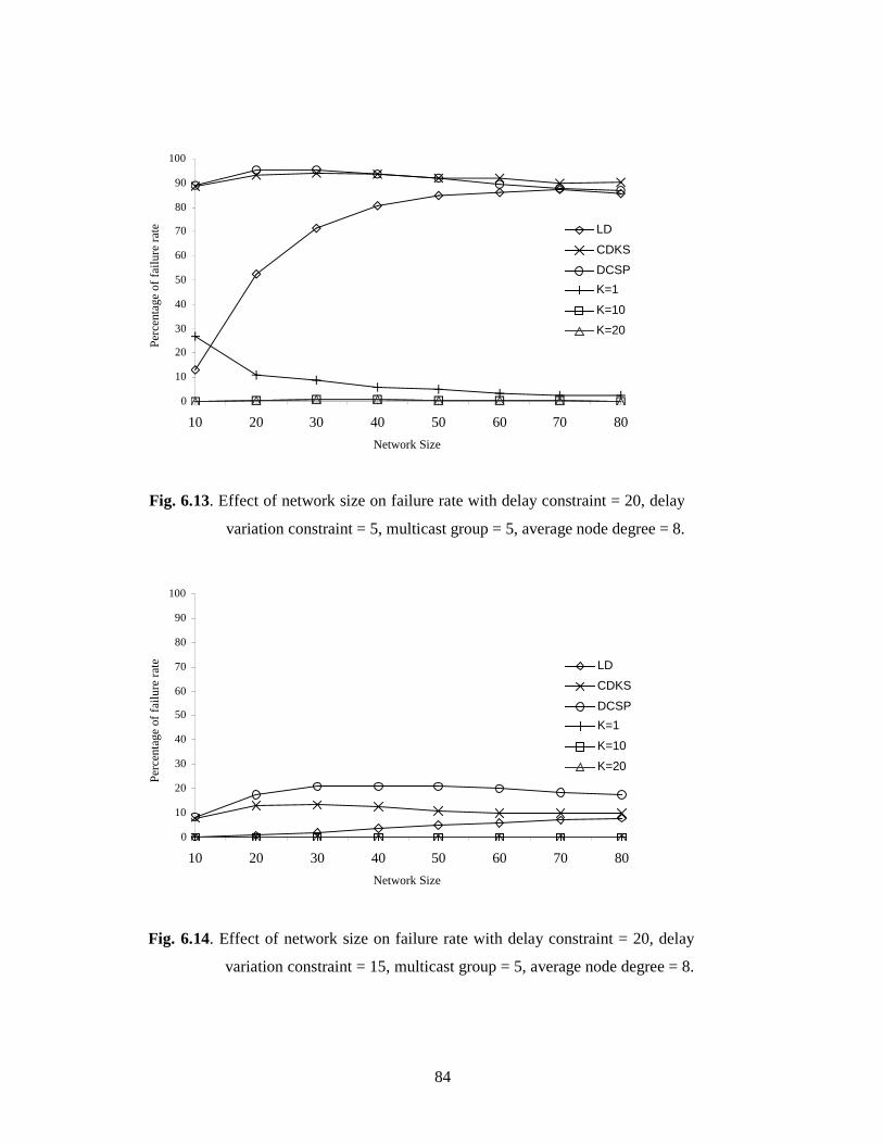
84
0
10
20
30
40
50
60
70
80
90
100
10 20 30 40 50 60 70 80
Network Size
Perc
enta
ge o
f fa
ilur
e ra
te LD
CDKS
DCSP
K=1
K=10
K=20
Fig. 6.13. Effect of network size on failure rate with delay constraint = 20, delay
variation constraint = 5, multicast group = 5, average node degree = 8.
Fig. 6.14. Effect of network size on failure rate with delay constraint = 20, delay
variation constraint = 15, multicast group = 5, average node degree = 8.
0
10
20
30
40
50
60
70
80
90
100
10 20 30 40 50 60 70 80
Network Size
Perc
enta
ge o
f fa
ilur
e ra
te LD
CDKS
DCSP
K=1
K=10
K=20

85
6.6.2 Average Cost per Path
Figures 6.15 and 6.16 investigate the effect of changing network size on the
average cost per path. The figures use the same parameters as in Figures 6.13 and
6.14.
In Fig. 6.15, we set the delay variation constraint � =5. DCSP always dominates
all other algorithms. The difference between DVCSP with K = 10 and K = 20 is very
small indicating again that K = 10 is sufficient for DVCSP. CDKS dominates DVCSP
at N < 30, with large network size, DVCSP dominates CDKS. This indicates that
DVCSP is more suitable in large network size. DVCSP with K = 1 gives a very high
cost compared to all other algorithms.
In Fig. 6.16, we relax the delay variation constraint to be 15 instead of 5. DCSP
still get the best results. DVCSP with K = 10 and K = 20 always dominates CDKS for
all different network sizes. It can be observed that DVCSP with K =1 is comparable
with CDKS and even dominates it at N > 30. This indicates that DVCSP works very
well in large network size and large delay variation.
Fig. 6.16. Effect of network size on average cost per path with delay constraint = 20,
delay variation constraint = 15, multicast group = 5, average node degree = 8.
130
140
150
160
170
180
190
200
210
10 20 30 40 50 60 70 80Network Size
Avg
. Cos
t/Pa
th
LD CDKS DCSPK=1 K=10 K=20

86
6.7 Conclusion
Large number of simulation experiments have been done to compare the
proposed DVCSP algorithm that is developed in chapter 5 for delay and delay
variation shortest path problem with other algorithms that is mainly for delay
constrained shortest path problem. We consider two performance factors, the failure
rate and the average cost per path. For the failure rate, DVCSP always dominates all
other algorithms with a very great difference. For the average cost per path, DVCSP
sometimes gives results that dominates LD and CDKS algorithms in case of large
degree and large network size. On the other side, DCSP algorithm, developed in
chapter 3, always dominates DVCSP in terms of cost. DVCSP suffers additional cost
which is paid for satisfying the additional constraint of delay variation. For all
simulated experiments, we choose to simulate DVCSP with three different values if K
which are 1, 10 and 20. Simulation results recommend that using K = 10 is almost has
the same results as in case of K = 20 while using K = 1 always results in a very high
cost which makes it not practical. So, K = 10 may be considered as a good value in
DVCSP algorithm.

87
Chapter 7
Conclusion and Suggestions for Future
Work
7.1 Conclusion
This thesis considers the problem of multicast routing under special constraints
that represent QoS parameters. A survey of current algorithms that deal with different
kinds of constraints is presented with other problems that is related to multicast
routing. The need for more algorithms for multicast routing problems was apparent. In
our work, we focus on two problems for multicast routing. The first problem is the
need for an algorithm for multicast routing in real-time networks. This meets the
requirements for the new applications like real time and multimedia applications. The
problem is formulated as delay constrained shortest path tree where we seek to
minimize the cost of each path from source to any destination while satisfying the
delay constraint. The second problem is that some applications like video
conferencing are not only in need to be real time but also a certain balance between
participants must be guaranteed. This balance is formulated as a delay variation
constraint and added to the delay constraint which results in a new problem that is
finding a shortest path route under delay and delay variation constraints. The two
studied problems are known to be an NP-Complete.
A new polynomial time heuristic algorithm, called DCSP, is proposed for the
delay constrained shortest path problem. The algorithm is discussed in depth aided
88
with flowcharts and pseudo code for its main subroutines. The correctness and
termination of the algorithm is proved. A complexity analysis of DCSP is also
proposed. An extensive analysis of DCSP performance is done by comparing it with
other algorithms via large number of simulation experiments that simulate real
networks. Simulation results show that DCSP always dominates the other algorithms
and its performance is increased at tight delay constraint and large average node
degree.
Another new polynomial time heuristic algorithm, called DVCSP, is proposed for
shortest path problem under delay and delay variation constraints. DVCSP uses a
variation of DCSP algorithm as its initial phase. Full discussion and analysis of
DVCSP algorithm is presented with flowcharts and pseudo code of its main
subroutines. Complexity analysis of DVCSP is investigated with the proof of its
termination. By using the same simulation environment that is used in simulating
DCSP algorithm, the performance analysis of DVCSP algorithm is investigated.
DVCSP is compared via other algorithms that is designed for delay constrained
problem. Two performance factors are considered, the failure rate to satisfy the delay
variation constraint and the average cost per path. DVCSP gives a very low failure
rate with respect to other algorithms. In addition, the cost of DVCSP is comparable to
other algorithms and even in sometimes dominates some algorithms. However, the
cost of DVCSP never dominates the cost of DCSP.
7.2 Suggestions for Future Work
The work of this thesis can be extended in several areas:
• The proposed algorithms are centralized which means that all data must be
stored in the source node. A need for a distributed implementation of these
algorithms will be valuable and more scalable in case of large network size,
where we will need that every node stores only a limited amount of
information.

89
• The dynamic change of multicast group members should be considered to be
embedded on the proposed algorithms so that we do not need to run the
algorithm from the beginning with every change in the multicast group.
• The proposed algorithms should be incorporated in an appropriate protocol to
be used in real networks.
• More constraints can be added to the proposed algorithms like the degree
constraint which is suitable to ATM networks.
• The proposed algorithms minimize the cost of each path individually which
results in a shortest path tree, similar work could be done in minimizing the
total cost of the multicast tree which is called minimum Steiner tree.
• The proposed algorithms deal with multicasting problems, similar work could
be done for broadcasting and unicast problems.

90
References
[1] S. Casner and S. Deer ing, “ First IETF Internet Audiocast,” in Proceedings of ACM
SIGCOMM, Computer Communications Review, vol. 22, no. 3, July 1992.
[2] R. Bellman, Dynamic Programming. Pr inceton University Press, 1957.
[3] J. Dossey, A. Otto, L. Spence, and C. Eynden Discrete Mathematics, Second Edition, Harper
Collins College Publishers, 1993
[4] A. Tanenbaum, Computer Networks, Third Edition. Pr intice-Hall International, Inc., 1996
[5] S. Deer ing and D. Cher iton, “ Multicast Routing in Datagram Internetworks and Extended
LANs” , ACM Transactions on Computer Systems, vol. 8, no. 2, pp. 85-110, May 1990.
[6] H. Salama, “ M ulticast Routing for Real-Time Communication on High-Speed Networks” ,
PhD. Disser tion, Nor th Carolina State University. Depar tment of Electr ical and Computer
Engineer ing, 1996.
[7] R. Widyono, “ The Design and Evaluation of Routing Algor ithms for Real-Time Channels” ,
Tech. Rep. ICSI TR-94-024, University of California at Berkeley, International Computer
Science Institute, June 1994.
[8] Q. Sun and H. Langendoer fre, “ Efficient Multicast Routing for Delay-Sensitive Applications” ,
in Proceedings of the second Workshop on Protocols for Multimedia Systems (PROMS’95), pp.
452-458, October 1995.
[9] S. Wi and Y. Choi, “ A Delay-Constrained Distr ibuted Multicast Routing Algor ithms” , in
Proceedings of the twelveth International Conference on Computer Communication
(ICCC’95), pp. 883-838, 1995.
[10] M. Garey, R. Graham, and D. Johnson, “ The complexity of computing steiner minimal
trees” , SIAM Journal of Applied Mathematics, vol. 32, no. 4, pp. 835-859, June 1977,
[11] P.Winter , “ Steiner Problem in Networks: A Survey” , Networks, vol. 17, no. 2, pp. 129-167,
summer 1987,
[12] F. Hwang and D. Richards, “ Steiner Tree Problems” , Networks, vol. 22, no. 1, pp 55-89,
January 1992.
[13] L. Kou, G. Markowsky, and L. Berman, “ A Fast Algor ithm for Steiner Trees” , Acta
Informatica, vol. 15, no. 2, pp 141-145, 1981.
[14] V. Kompella, J. Pasquale, and G. Polyzos, “ Multicasting for Multimedia Applications” , in
Proceedings of IEEE INFOCOMM’92, pp. 2078-2085, 1992.
[15] V. Kompella, J. Pasquale, and G. Polyzos, “ M ulticast Routing for Multimedia
Communication” , IEEE/ACM Transactions on Networking, vol.1, no. 3, pp 286-292,June
1993.

91
[16] C. Noronha and F. Tobagi, “ Optimum Routing of Multicast Streams” , in Proceedings of
IEEE INFOCOM’94, pp 865-873, 1994.
[17] Q. Zhu, M . Parsa, and J. Garcia-Luna-Aceves, “ A Source-Based Algor ithm for Delay-
Constrained Minimum-Cost Multicasting” , in Proceeding of IEEE INFOCOM’95, pp. 337-
385, 1995.
[18] M. Parsa, Q. Zhu, and J. Garcia-Luna-Aceves, “ An I terative Algor ithm For Delay-
Constrained Minimum-Cost Multicasting” , IEEE/ACM Transactions on Networking, vol.6,
no.4, August 1998.
[19] Q. Sun and H. Langendoerfre, “ An Efficient Delay-Constrained Multicast Routing
Algor ithm” , journal of High Speed Networks Vol. 7 No. 1 1998
[20] V. Kompella, J. Pasquale, and G. Polyzos, “ Two Distibuted Algor ithms for the Constrained
Steiner Tree Problem” , in Proceedings of the second International conference on Computer
Communications and Networking (ICCCN’93), pp 343-349, 1993.
[21] M . Parsa, “ Multicast Routing in Computer Networks” , PhD. Disser tion, University of
California, Santa Cruz, Computer Engineer ing, June 1998.
[22] Y. Im and Y. Choi, “ A Distr ibuted Multicast Routing with End-to-End Delay Bound” in
Proceeding of SEACOMM, Penang, August1998.
[23] X. Jia, “ A Distibuted Algor ithm of Delay-Bounded Multicast Routing for Multimedia
Applications in Wide Area Networks” , IEEE/ACM Transactions on Networking, vol. 6, no.
6, pp 828-837, December 1998.
[24] Y. Lee, Y. Im, K . Lee and Y. Choi, “ A Bandwidth and Delay constrained M inimum Cost
M ulticast Routing Algor ithm” in Proceeding of ICOIN-11, Taipei, Jan. 1997.
[25] G. Rouskas and I . Baldine, “ M ulticast Routing with End-to-End Delay and Delay Var iation
Constraints” , IEEE Journal of Selected Areas in Communications, vol.15, no.3, pp 346-356,
Apr il 1997.
[26] B. Haberman and G. Rouskas “ Cost, Delay, And Delay Var iation Conscious Multicast
Routing” , Tech. Rep. TR-97-03, Depar tment of Computer Science, North Carolina State
University, March 1996.
[27] B. Haberman “ Cost, Delay, And Delay Var iation Conscious Multicast Routing” , Master
Thesis, Depar tment of Computer Science, North Carolina State University, March 1997.
[28] H. Tode, Y. Sakai, H. Okada and Y. Tezuka, “ M ulticast Routing Algor ithm for Nodal Load
Balancing” , in Proceedings of IEEE INFOCOM’92, pp 2086-2095, 1992.
[29] F. Bauer and A. Verma “ Degree-Constrained Multicasting in Point-to-Point Networks” , in
Proceedings of IEEE INFOCOM’95, pp 369-376, 1995.
[30] F. Bauer “ Multicast Routing in Point-to-Point Networks Under Constraints” , PhD
Disser tion, University of California, Santa Cruz, Computer Engineer ing June 1996.
[31] M. Ammar, S. Cheung, and C. Scoglio “ Routing M ultipoint Connections Using Vir tual
Paths in an ATM Networks” , in Proceedings of IEEE INFOCOM ’93, pp 98-105, 1993.
[32] B. Waxman, “ Routing of M ultipoint Connections” , IEEE Journal on Selected Areas of
Communication, Vol. 6, No. 9, pp. 1617-1622 December 1988.

92
[33] F. Bauer and A. Verma “ ARIES: A Rearrangeable Inexpensive Edge-Based On-L ine
Steiner Algor ithm” , IEEE Journal of Selected Areas in Communications, vol.15, no.3, pp
382-397, Apr il 1997.
[34] E. Biersack and J. Nonnenmacher , “ WAVE: A new Multicast Routing Algor ithm for Static
and Dynamic M ulticast Groups” , in Proceedings of the Fifth International Workshop on
Network and Operating System Support for Digital Audio and Video, pp 228-239, 1995.
[35] Q. Sun and H. Langendoerfer , “ A Distr ibuted Delay-Constrained Dynamic Multicast
Routing Algor ithm” , in Proceedings of European Workshop on Interactive Distributed
Multimedia Systems and Telecommunication Services (IDMS'97) Vol. 1309, pp.97-106, 1997
[36] A. Geol and K . Munagala, “ Extending Greedy Multicast Routing to Delay Sensetive
Applications” , Tech. Rep. CS-TN-99-89, Stanford University, Deapr tment of Computer
Science, July 1999.
[37] H. Salama, D. Reeves and Y. Viniotis, “ A Distr ibuted Algor ithm for Delay-Constrained
Unicast Routing” , in Proceeding of IEEE INFOCOM’97, Apr il 1997.
[38] H. Salama, D. Reeves and Y. Viniotis, “ The Delay-Constrained Minimum Spanning Tree
Problem” , IEEE in Proceeding of Second IEEE Symposium on Computers and
Communications (ISCC’97), Alexandria, Egypt, July 1997.
[39] C. Noronha and F. Tobagi, “ Evaluation of Multicast Routing Algor ithms for Multimedia
Streams” , in Proceedings of IEEE International Telecommunications Symposium, August
1994.
[40] H. Salama, D. Reeves and Y. Viniotis, “ Evaluation of M ulticast Routing Algor ithms for
Real-Time Communication on High-Speed Networks” , IEEE Journal on Selected Areas of
Communication, Vol. 15, No. 3, pp. 332-345 Apr il 1997.
[41] C. Diot, W. Dabbous and J. Crowcroft, “ Multipoint Communication: A Survey of Protocols,
Functions, and Mechanisms” , IEEE Journal on Selected Areas of Communication, Vol. 15,
No. 3, pp. 277-290 Apr il 1997.

93
APPENDIX A : Pseudo Code of DCSP Algor ithm
In this appendix we present the pseudo code for DCSP algorithm with its two main subroutines that were described in chapter 3.
A.1 Pseudo Code for DCSP algor ithm
/* Delay Constrained Shortest Path Algorithm based on
Flooding mechanism, the input to the algorithm is:
1 - Graph G with nodes V and links E, G (V, E), to describe the
network topology.
2 - Source Node S
3 - Multicast Group M
4 - Delay Constraint ∆∆∆∆
5 - Constant K, Maximum Number of tokens in any node.
The algorithm outputs a subgraph G` which is either tree or directed acyclic graph and
it contains all the links needed for routing in the shortest path. The graph G (V, E) is
represented as a two dimensional array* /
Graph DCSP ( G(V,E) , S , M , ∆∆∆∆ , K )
{
Insert a token in S
/* Each token contains three fields, Delay(T), the token delay so far,
Cost(T), the token cost so far and an array of stamps that keeps track of
the nodes that token passed so far. At the first token Delay(T) = 0,
Cost(T) = 0 and the array of stamps contains only the stamp of the
source node*/
No. Of Tokens = 1
While ( No. of Tokens > 0 )

94
{
for each Node u in V
{
for each Token T currently in Node u
{
for each neighbor Node v to Node u
{
if Can_Duplicate ( T , u , v )
{
Duplicate_Token ( T , u , v)
I f Node v ∈ M
Update the winner Token of node v
/* The winner token is the token that reaches
the destination with lower Cost(T) and
Delay(T) < ∆ * /
} /* For Can_Duplicate * /
} /* For neighbor node v * /
No. Of Tokens = No. Of Tokens – 1
} /* For Token T * /
} /* For node u * /
} /* For While * /
for each Node u in M
Insert all links that the winner Token for u passed in subgraph G`
Return G`
} /* For DCSP * /
A.2 Pseudo Code for Function Can_Duplicate(T,u,v)
/* Function Can_Duplicate takes the input :
1 - Token T
2 - The Node u that currently holds the token
3 – The Node v that the token needs to be duplicated in.

95
Then the function outputs either False when the Token T can’ t be duplicated from u
to v or True when the token can safely be duplicated from u to v * /
Boolean Can_Duplicate ( T , u , v )
{
/* If the token will exceed the delay limit, we will not duplicate it * /
if ( Delay(T) + Delay ( u , v ) ) > ∆
Return False
/* If the token will make a loop, we will not duplicate it * /
if Node v stamped Token T before
Return False
/* If we got a better token before, we will not duplicate the token, this can be
achieved by comparing the current token by the history kept at node v to see if there
was a better token in terms of delay and cost w.r.t current token or not* /
if Node v got a better token before
Return False
/* If there is no room for the new token, we will not duplicate it * /
/* We limit the number of tokens that can be kept by any node by the number K.
So, if we have a new token after the first K, we have to choose a victim from the K+1
tokens. Our heuristic is to choose the token with the highest delay * /
if there are K tokens in Node v
if Token T has the highest delay among all tokens in node v
Return False
Else
Delete the token that has the maximum delay among all
tokens in
node v
/* Now the Token T is valid for duplication, and we have to put it in the
history of Node v as one of the best tokens so far * /

96
/* If the history is full, we have to remove one of the old entries in this
history. Our heuristic is to remove the entry with the highest delay * /
I f the history list of node v has K entries
Delete the one with the highest delay
Insert Token T in the history list of Node v
Return True
} /* for Can_Duplicate * /
A.3 Pseudo Code for Procedure Duplicate_Token(T,u,v)
/* Procedure Duplicate_Token is used to duplicate Token T from Node u to
Node v , the procedure has three inputs:
1 - Token T that needs to be duplicated
2 - The Node u that currently holds the token
3 – The Node v that the token needs to be duplicated in.
* /
Duplicate_Token ( T , u , v )
{
/* Update the token cost and delay * /
Cost(T) = Cost(T) + Cost ( u , v )
Delay(T) = Delay(T)+ Delay ( u , v )
Node v puts its stamp on Token T
No. Of Tokens = No. Of Tokens + 1
}

97
APPENDIX B : Pseudo Code of DVCSP Algor ithm
In this appendix we present the pseudo code for DVCSP algorithm with its main subroutines that were described in chapter 5.
B.1 Pseudo Code for DVCSP algor ithm
/* Delay and Delay Variation Constrained Shortest Path
Algorithm, the inputs to the algorithm are:
6 - Graph G with nodes V and links E, G (V, E), to describe the
network topology.
7 - Source Node S
8 - Multicast Group M
9 - Delay Constraint ∆∆∆∆
10 - Delay Variation Constraint
11 - Constant K, Maximum Number of tokens in any node.
The algorithm outputs a subgraph G` which is either tree or directed acyclic graph and
it contains all the links needed for routing in the shortest path. The graph G (V, E) is
represented as a two dimensional array* /
Graph DVCSP ( G(V,E) , S , M , ∆∆∆∆ , , K )
{
Delay_Constraint_Phase( G(V,E) , S , M , ∆∆∆∆, K )
for each node m in M
I f there is no tokens in m
return failure to satisfy the delay constraint.

98
Graph = Delay_Variation_Constraint_Phase( M , )
for each node m in M
I f there is no tokens in m
return failure to satisfy the delay variation constraint.
return Graph
}
B.2 Pseudo Code for Phase I : Delay_Constraint_Phase
/* Phase I: Delay Constraint Phase takes the input:
1- Graph G with nodes V and links E, G (V, E), to describe the
network topology.
2- Source Node S
3- Multicast Group M
4- Delay Constraint ∆∆∆∆
5- Constant K, Maximum Number of tokens in any node.
This phase divides the interval [0, �] into K segments with equal size � / K where
each node u can have only one token in each segment. This phase outputs at most 3K
tokens for each node m ∈ M where each segment can contain only the results of three
tokens, the least delay, highest delay and the least cost token. * /
Delay_Constraint_Phase ( G(V,E) , S , M , ∆∆∆∆ , K )
{
Insert a token in S
/* Each token contains three fields, Delay(T), the token delay so far,
Cost(T), the token cost so far and an array of stamps that keeps track of
the nodes that token passed so far. At the first token Delay(T) = 0,

99
Cost(T) = 0 and the array of stamps contains only the stamp of the
source node*/
No. Of Tokens = 1
While ( No. of Tokens > 0 )
{
for each Node u in V
{
for each Token T currently in Node u
{
for each neighbor Node v to Node u
if Can_Duplicate ( T , u , v ) Duplicate_Token ( T , u
, v, M)
No. Of Tokens = No. Of Tokens – 1
} /* For Token T * /
} /* For node u * /
} /* For While * /
} /* For Delay_Constraint_Phase * /
B.3 Pseudo Code for Function Can_Duplicate(T, u, v)
/* Function Can_Duplicate takes the input :
1 - Token T
2 - The Node u that currently holds the token
3 – The Node v that the token needs to be duplicated in.
The function outputs either False when the Token T can not be duplicated from u to v
or True when the token can safely be duplicated from u to v * /
Boolean Can_Duplicate ( T , u , v )
{
/* If the token will exceed the delay limit, we will not duplicate it * /
if ( Delay(T) + Delay ( u , v ) ) > ∆
Return False

100
/* If the token will make a loop, we will not duplicate it * /
if Node v stamped Token T before
Return False
/* Calculate the segment that token T wants to duplicate in * /
Segment_no = (Delay(T) * K ) / �
/* Each token should keep at most one token in each segment * /
if node v has another token T1 in the segment Segment_no
/* According to our heuristic, if two tokens want to
duplicate at the same time in the same segment in the same
node, we choose the token with least delay * /
if (Delay(T1) < Delay(T))
Return False
else
Delete token T1
Return True
} /* for Can_Duplicate * /
B.4 Pseudo Code for Procedure Duplicate_Token(T, u ,v, M)
/* Procedure Duplicate_Token is used to duplicate Token T from Node u to
Node v , the procedure has four inputs:
1 - Token T that needs to be duplicated 2 - The Node u that currently
holds the token
3 – The Node v that the token needs to be duplicated in. 4- Multicast Group M * /
Duplicate_Token ( T , u , v, M )
{
/* Update the token cost and delay * /

101
Cost(T) = Cost(T) + Cost ( u , v )
Delay(T) = Delay(T)+ Delay ( u , v )
Node v puts its stamp on Token T
No. Of Tokens = No. Of Tokens + 1
/* if node v is in multicast group, we will update the least delay, highest delay and least cost tokens
kept at the segment that token T wants to duplicate in. * /
if ( v ∈ M )
{
/* Calculate the segment that token T wants to duplicate in * /
Segment_no = ( (Delay(T) + Delay (u , v)) * K ) / �
/* Compare the duplicated token with the least delay token in
this segment and if it is better, replace the old one* /
if (Delay(T) < Least_Delay[ Segment_no] )
Least_Delay[ Segment_no] ) = Delay(T)
/* Compare the duplicated token with the highest delay token in this segment
and if it is better, replace the old one*/
if (Delay(T) > Highest_Delay[ Segment_no] )
Highest_Delay[ Segment_no] ) = Delay(T)
/* Compare the duplicated token with the least cost token in this
segment and if it is better, replace the old one* /
if (Cost(T) < Least_cost[ Segment_no] )
Least_cost[Segment_no] ) = Cost(T)
} /* for if condition * /
} /* for Duplicate_Token * /
B.5 Pseudo Code for Phase I I : Delay_Variation_Constraint_Phase
/*This phase is responsible for satisfying the delay variation constraint, given that all
the examined tokens in this phase are already satisfy the delay constraint. This phase
has two inputs :
1- Multicast Group M
2- Delay Variation Constraint
The phase returns a subgraph G` which is either tree or directed acyclic graph and
contains all the links needed for routing in the shortest path. * /

102
Graph Delay_Variation_Constraint_Phase ( M , )
{
/* Collect all the tokens that kept in each node u ∈ M in one array called
merged_array which is sorted in ascending order according to the delay of each
token* /
for each node u ∈ M
for each segment segment_no in node u
{
Insert the token least_delay[ segment_no] into merged_array.
Insert the token highest_delay[segment_no] into merged_array.
Insert the token least_delay[segment_no] into merged_array.
}
start_pointer = 0
for each token T in merged_array
{
/* We should keep track of start_pointer and end_pointer such that the
difference between the delay of the tokens at start_pointer and
end_pointer satisfy the delay variation constraint * /
end_pointer = start_pointer
Ts = The token that start_pointer points to
Te = The token that end_pointer points to
D = The destination that we got Te from
total_cost = 0
best_cost = �
Set all elements in cost_window array to �
/* Advance Te till it violates the delay variation constraint * /
while (Delay(Te) – Delay(Ts) < � )
{
/* We will check all the tokens that lie between Ts and
Te. If this goup of tokens contain at least one token from
each destination, then we got a solution and we will
compare it with the best solution we got before. If this

103
group of token does not contain any token from a certain
node, so there is no solution in this interval. * /
if (cost_window[D] = � )
{
/* This is the first token found in the interval
[Ts, Te] that represents the destination node D * /
total_cost = total_cost + Cost(Te)
cost_window[ D] = Cost[Te]
}
else
{
/* Destination D had a token before in
interval [Ts , Te], so, we will compare this
token by the new token and choose the least
cost one * /
if ( cost_window[D] > Cost(Te) )
{
total_cost = total_cost –
cost_window[ D] + Cost(Te)
cost_windoe[D] = Cost[ Te]
}
}
end_pointer = end_pointer + 1
}
/* Check if the interval [Ts, Te] covers all the destination or not. * /
if cost_window does not contain �
{
/* The interval [Ts, Te] covers all the destination, so, we will check
whether the total cost of the tokens so far is the best one or not * /
if (total_cost < best_cost)
{
best_cost = total_cost
best_window = cost_window

104
}
}
start_pointer = start_pointer + 1
} /* for For Loop * /
if best_window contain �
return failure to satisfy delay variation constraint
else
The returned graph is the union of all paths constituting the tokens in
best_window
} /* for Delay_Var iation_Constraint_Phase * /
B.6 Pseudo Code for Procedure Get_Minimum_Variation (M)
/* This procedure is executed only when phase II failed to satisfy the delay variation
constraint. The procedure returns a subgraph with the minimum possible delay
variation * /
Graph Get_Minimum_Variation ( M )
{
start_pointer = 0
Ts = The token that start_pointer points to
D = The destination that we got Te from
best_delay = �
Set all elements in best_window array to � for each token T in merged_array
{
delay_window[ D] = Delay(Ts)
if (delay_window does not contain �)
{
/* The maximum variation can be calculated by calculating the maximum and
minimum values in delay_window array and get their difference * /
Var = calculate the maximum variation in delay_window
If (Var < best_delay)
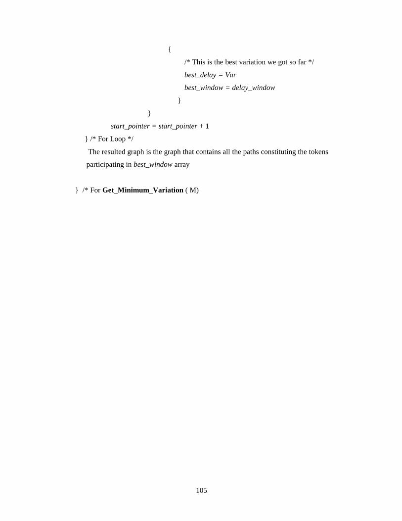
105
{
/* This is the best variation we got so far * /
best_delay = Var
best_window = delay_window
}
}
start_pointer = start_pointer + 1
} /* For Loop * /
The resulted graph is the graph that contains all the paths constituting the tokens
participating in best_window array
} /* For Get_Minimum_Var iation ( M)

106
�������� ������������� ����������������� !� � �"� ��#��$%�&��'(���)*+�,(��-
�.��/���01$���2�)����3���45�'$�����6�)�3��3���)� ���������7����8'�9-������2����/���01$��
&�5(3���2�&�-$:�����(3-;3���<=�>
? �,(��3���@2A��B#��$����C�? �2�@$D2�E�3F�G��<�����<���&D�����&/������<���-���H�C�
����012������I�����>�<���&D�����&/������<���-���H�C�?���,(��3����I�=���B#��$������J
� ���01$������K��/���� L �MJ�E�3F�N�*O�2� ����012������I�����@$D2�E�3F�G��<����
�����P� 6� ������� �9QH�RJ>
��S��9-�������O� ��T��2�U�$�J�V�'���H�&��'(�W
��$:�3���2� �������������$:�3���,(�2�&��'(���X$F$3��&�/�%�S ��-�S-�@2!��U�����
�C�?���Y�F$-�S-�N�*O�2�����T���01$���������� ������������� ������������3������ Z�
�?3�[9-�V�/�O�2�&��'(��� �>
I�=���U�������S-��1�2�2� ������������� ���������@�������&���������'������\ (6��
�<���] ����,(�G��X$I�<O����&�����������#��$����\ (6�G��X�$IJ���6���H��?/�9:-
B#��$%�<O���L�3��2�U$�6�&����̂TF$��B#��$%>
������� ����������������� !�,(��3���@2A��B#��$����\ (6����=���U�������S-��1�2
�������I�����@$D2�E�3F�G��<�����<���VD�����&/������<���-���H�C�? �R*���2� �����
����012�>�)����-�V"���,(�G��,(��3���B#��$������ �������I�����<��+�\ (6�S-�N�*O�2
&�TD���QH�2>
&�I�����_ (̀ � 6�,(��3���@2A��B#��$�����a�/���<��T-�<36�G��(���U�������S-��1�2�
�U���-� ��(�O���6�_ (̀ � 6�N�b�2�V��c3���d/I�<T��&�����3���&�����������#��$����
V����T������c����O�T-������)�O�T3��>
������� ����������������� !�,(��3����I�=���B#��$����\ (6�d������U�������S-��1�2
��<�����<���&D�����&/������<���-���H�C�? �R*���2� ������������I�����@$D2�E�3F�G

107
�����P� 6� ������� �9QH�RJ� ���01$������K��/���� L �MJ�E�3F�N�*O�2� ����012�>�S-��3O
)����-�V"���,(�G��,(��3���B#��$������ �������I�����<��+�\ (6>
�&�I�����_ (̀ � 6�,(��3����I�=���B#��$�����a�/���<��T-�<36�S-�e������U������
��$�����2�,(��3���@2A��B#��$�����&�I�����N�*O�2�G��(���U��������?-�O�T��03-����������#
V����T������c����O�T-������)�O�T3���U���-� ��(�O���6�_ (̀ � 6�N�b>
�&D�������P�(�1!��\ (6�G��V��'(���f5��9��] ���-�2�\ (6�G������U����.��S-��1�2
H� �3 ������&�����3���@�36A��&��'(���X$F$3���?���F>
��I�=���_T�3���<�J�,(��3���@2A��B#��$�������:/-�gD2�\ (6�S-�@2A��_T�3�����2
,(��3����I�=���B#��$�������:/-�gD2���6�R$�T��>

108
V ��9�'!��V���"
V'�9?���V��O
.�h��S�T����2�V'�T����Mh��S�1
V�����V��'� (���"�3���V"�����6�@$:T���.5L"�#��IZO
�
C�(H�0T- �$�O����b��'A��i�9 �����& LI��3T�
)�$�O����i4 $T����3T��@�3O��3PJ�a��2
V ��9�'!� jkkk
Top Related