


Languages
Pages
Legal


Advanced MeasuresAdvanced Measures
Mike Davies, MD FACPMike Davies, MD FACPMark Murray and AssociatesMark Murray and Associates

Where we’re going….Where we’re going….
• Compass: Examples of Compass: Examples of systemizationsystemization
• Analysis to answer questionsAnalysis to answer questions– RunRun– SPCSPC– QueuingQueuing– ModelingModeling


Dr Provider #1: “warm and compassionate with patients, infinite patience with some of the toughest customers”

Is There an Access Problem?
Does this Provider have sufficient Access Availability?
• Yes for sure!• Yes I think so• I am not sure• I don't think so• Absolutely not!
Quiz
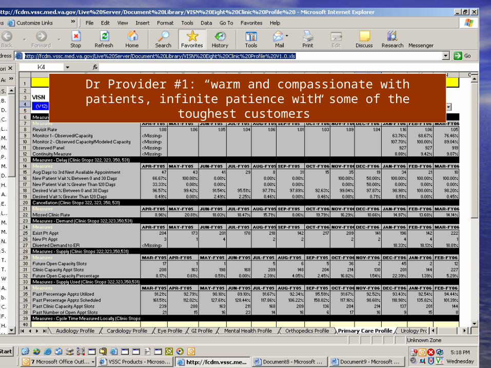
Dr Provider #1: “warm and compassionate with patients, infinite patience with some of the toughest customers”

Does Provider #1 Have Adequate Access?
– Provider #1 Third next available: >7 days in all months!Provider #1 Third next available: >7 days in all months!
– Provider #1 CUSS Past percentage appts utilized: >90% in 11 of 12 monthsProvider #1 CUSS Past percentage appts utilized: >90% in 11 of 12 months
• (Dis) Continuity Measure < 10% (may depend upon facility/ Primary Care (Dis) Continuity Measure < 10% (may depend upon facility/ Primary Care structure)structure)– Provider #1 Continuity: 9%Provider #1 Continuity: 9%
• Diverted Demand to ER < 10%Diverted Demand to ER < 10%– Provider #1: 18%Provider #1: 18%

Does Provider #1 Have Adequate Access?
• No!!No!!– Uniformly poor Access Availability Uniformly poor Access Availability
throughout the entire year, with few throughout the entire year, with few available slots and a high third next available slots and a high third next available.available.
Diagnosing Access Problems
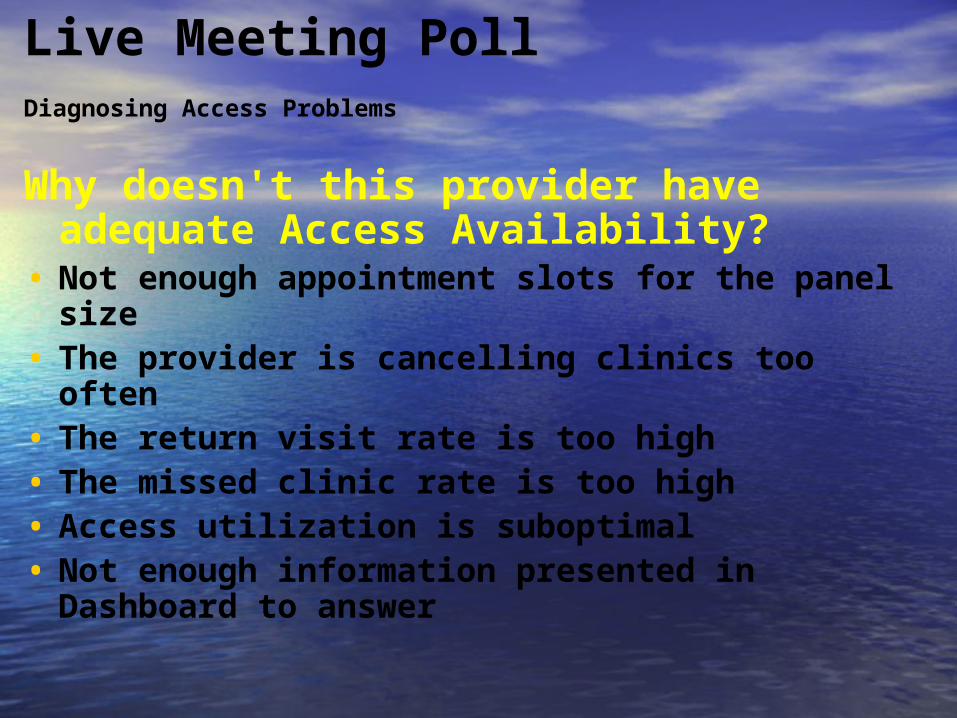
Why doesn't this provider have adequate Access Availability?
• Not enough appointment slots for the panel size• The provider is cancelling clinics too often• The return visit rate is too high• The missed clinic rate is too high• Access utilization is suboptimal• Not enough information presented in Dashboard to
answer
Live Meeting Poll
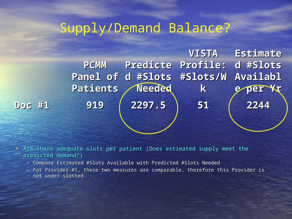
PCMM PCMM Panel of Panel of PatientsPatients
Predicted Predicted #Slots #Slots NeededNeeded
VISTA VISTA Profile: Profile:
#Slots/Wk#Slots/Wk
Estimated Estimated #Slots #Slots
Available Available per Yrper Yr
Doc #1Doc #1 919919 2297.52297.5 5151 22442244
Supply/Demand Balance?
• Are there adequate slots per patient (Does estimated supply meet the predicted Are there adequate slots per patient (Does estimated supply meet the predicted demand?)demand?)– Compare Estimated #Slots Available with Predicted #Slots NeededCompare Estimated #Slots Available with Predicted #Slots Needed– For Provider #1, these two measures are comparable, therefore this Provider is not under-For Provider #1, these two measures are comparable, therefore this Provider is not under-
slotted.slotted.
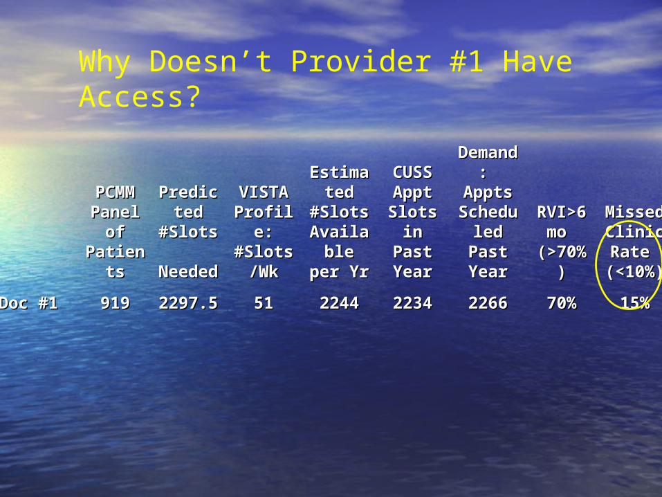
PCMM PCMM Panel Panel
of of PatientPatient
ss
PredictPredicted ed
#Slots #Slots NeededNeeded
VISTA VISTA Profile: Profile: #Slots/#Slots/
WkWk
EstimatEstimated ed
#Slots #Slots AvailabAvailable per le per
YrYr
CUSS CUSS Appt Appt
Slots in Slots in Past Past YearYear
DemanDemand: d:
Appts Appts SchedulScheduled Past ed Past
YearYear
RVI>6RVI>6mo mo
(>70%)(>70%)
Missed Missed Clinic Clinic Rate Rate
(<10%)(<10%)
Doc #1Doc #1 919919 2297.52297.5 5151 22442244 22342234 22662266 70%70% 15%15%
Why Doesn’t Provider #1 Have Access?

Other ways to use the Other ways to use the compasscompass
• Relative comparisonsRelative comparisons
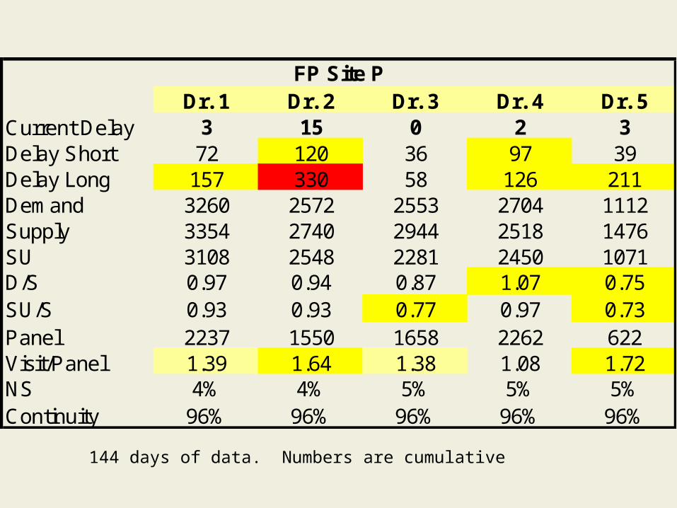
Dr. 1 Dr. 2 Dr. 3 Dr. 4 Dr. 5Current Delay 3 15 0 2 3Delay Short 72 120 36 97 39Delay Long 157 330 58 126 211Demand 3260 2572 2553 2704 1112Supply 3354 2740 2944 2518 1476SU 3108 2548 2281 2450 1071D/S 0.97 0.94 0.87 1.07 0.75SU/S 0.93 0.93 0.77 0.97 0.73Panel 2237 1550 1658 2262 622Visit/Panel 1.39 1.64 1.38 1.08 1.72NS 4% 4% 5% 5% 5%Continuity 96% 96% 96% 96% 96%
FP Site P
144 days of data. Numbers are cumulative
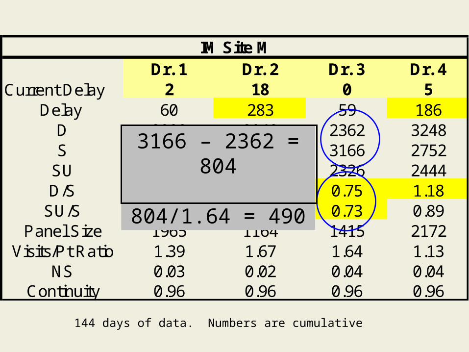
Dr. 1 Dr. 2 Dr. 3 Dr. 4Current Delay 2 18 0 5
Delay 60 283 59 186D 2999 2049 2362 3248S 3268 2229 3166 2752
SU 2723 1941 2326 2444D/S 0.92 0.92 0.75 1.18
SU/S 0.83 0.87 0.73 0.89Panel Size 1965 1164 1415 2172
Visits/Pt Ratio 1.39 1.67 1.64 1.13NS 0.03 0.02 0.04 0.04
Continuity 0.96 0.96 0.96 0.96
IM Site M
144 days of data. Numbers are cumulative
3166 – 2362 = 804
804/1.64 = 490
144 days of data. Numbers are cumulative
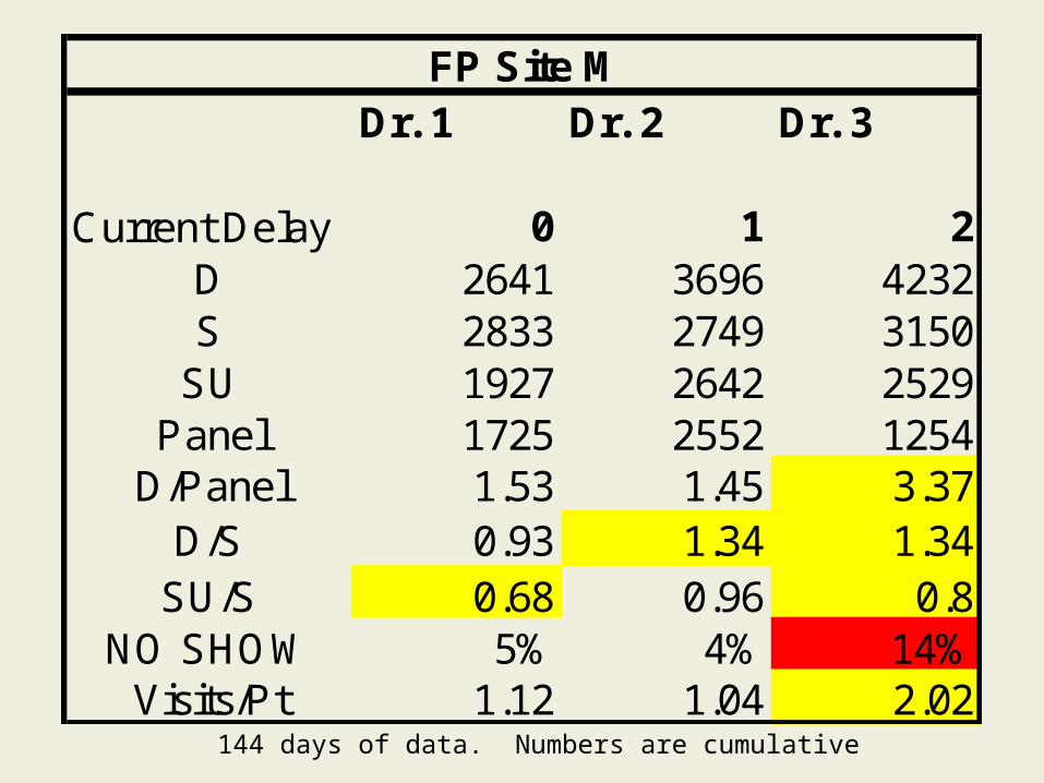
Dr. 1 Dr. 2 Dr. 3
Current Delay 0 1 2D 2641 3696 4232S 2833 2749 3150
SU 1927 2642 2529Panel 1725 2552 1254
D/Panel 1.53 1.45 3.37D/S 0.93 1.34 1.34
SU/S 0.68 0.96 0.8NO SHOW 5% 4% 14%
Visits/Pt 1.12 1.04 2.02
FP Site M
When we don’t interpret When we don’t interpret variation correctly…..variation correctly…..
• We see We see trendstrends when there are none when there are none
• We explain We explain natural variation as special natural variation as special eventsevents
• We We blame blame or or give creditgive credit when it’s when it’s undeservedundeserved
• We don’t understand We don’t understand past performancepast performance or make accurate or make accurate future predictionsfuture predictions
• Ability to Ability to make improvementsmake improvements is limited is limited
Two Types of VariationTwo Types of Variation
• Common CauseCommon Cause– Inherent in current design of processInherent in current design of process– Predictable - stablePredictable - stable– Due to “random chance”Due to “random chance”
• Special CauseSpecial Cause– Not inherent in process design – “unnatural”Not inherent in process design – “unnatural”– Unpredictable – unstableUnpredictable – unstable– Due to explainable causeDue to explainable cause
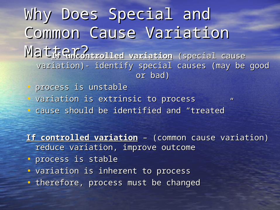
Why Does Special and Why Does Special and Common Cause Variation Common Cause Variation Matter?Matter?If uncontrolled variationIf uncontrolled variation (special cause variation)- (special cause variation)-
identify special causes (may be good or bad)identify special causes (may be good or bad)
• process is unstableprocess is unstable
• variation is extrinsic to processvariation is extrinsic to process
• cause should be identified and “treated”cause should be identified and “treated”
If controlled variationIf controlled variation – (common cause variation) – (common cause variation) reduce variation, improve outcomereduce variation, improve outcome
• process is stableprocess is stable
• variation is inherent to processvariation is inherent to process
• therefore, process must be changedtherefore, process must be changed

Can a Run Chart Detect Special Can a Run Chart Detect Special Cause Variation? ---- YES!Cause Variation? ---- YES!
• 1. Too many or too few runs1. Too many or too few runs– One or more data points on the same side of One or more data points on the same side of
the medianthe median– Do not include points ON the medianDo not include points ON the median
• 2. Shift: If more than 7-8 points in a run2. Shift: If more than 7-8 points in a run
• 3. Trend: If more than 5-6 consecutive 3. Trend: If more than 5-6 consecutive points up or downpoints up or down
• 4. Stratification: See-saw pattern4. Stratification: See-saw pattern

What is a Run?What is a Run?
• One or more consecutive data points One or more consecutive data points on the same side of the median.on the same side of the median.
• Do not include points ON the median Do not include points ON the median in a run.in a run.
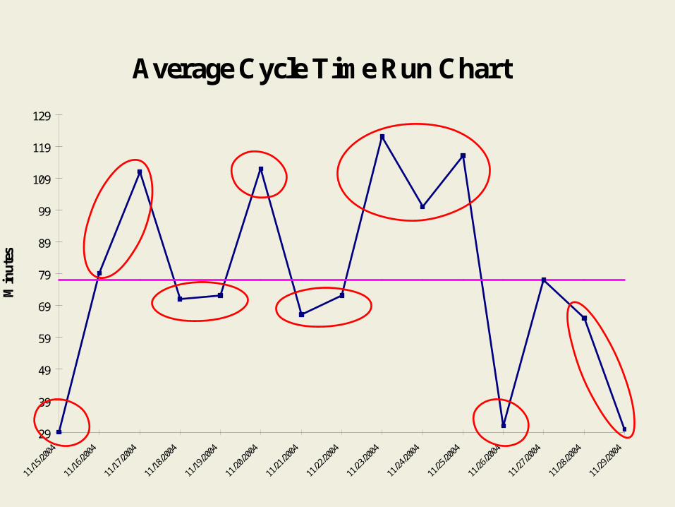
Average Cycle Time Run Chart
29
39
49
59
69
79
89
99
109
119
129
11/1
5/200
4
11/1
6/200
4
11/1
7/200
4
11/1
8/200
4
11/1
9/200
4
11/2
0/200
4
11/2
1/200
4
11/2
2/200
4
11/2
3/200
4
11/2
4/200
4
11/2
5/200
4
11/2
6/200
4
11/2
7/200
4
11/2
8/200
4
11/2
9/200
4
Min
utes

Useful Useful ObservationsObservations
Lower Lower LimitLimit
Upper Upper LimitLimit
1010 33 88
1111 33 99
1212 33 1010
1313 44 1010
1414 44 1111
1515 44 1212
1616 55 1212
1717 55 1313
1818 66 1313
1919 66 1414
2020 66 1515
2121 77 1515
2222 77 1616
2323 88 1616
2424 88 1717
2525 99 1717

Average Cycle Time Run Chart
29
39
49
59
69
79
89
99
109
119
129
11/1
5/200
4
11/1
6/200
4
11/1
7/200
4
11/1
8/200
4
11/1
9/200
4
11/2
0/200
4
11/2
1/200
4
11/2
2/200
4
11/2
3/200
4
11/2
4/200
4
11/2
5/200
4
11/2
6/200
4
11/2
7/200
4
11/2
8/200
4
11/2
9/200
4
Min
utes
Summary of Key PointsSummary of Key Points
• Become expert at creating run charts Become expert at creating run charts (it’s not that hard!)(it’s not that hard!)
• Use run charts to tell us if a change is Use run charts to tell us if a change is an improvementan improvement
• Use run charts to detect common and Use run charts to detect common and special causes of variationspecial causes of variation
• Post run charts widely so all can see Post run charts widely so all can see the changes!the changes!
Analyzing Variation – The Analyzing Variation – The MRI!MRI!
• Control Charts (or SPC charts)Control Charts (or SPC charts)– More sensitive than run charts More sensitive than run charts
•Common/Special CauseCommon/Special Cause
– Define process capabilityDefine process capability– Allow predictions of process behaviorAllow predictions of process behavior– Can be easily created by simply Can be easily created by simply
analyzing the data in a run chart with analyzing the data in a run chart with more sensitive formulasmore sensitive formulas
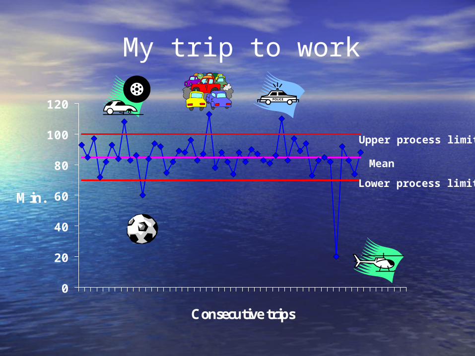
0
20
40
60
80
100
120
Consecutive trips
Min.
My trip to work
Mean
Upper process limit
Lower process limit
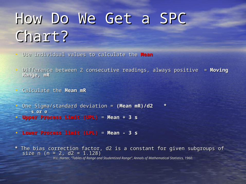
How Do We Get a SPC How Do We Get a SPC Chart?Chart?• Use individual values to calculate the Use individual values to calculate the MeanMean
• Difference between 2 consecutive readings, always positive Difference between 2 consecutive readings, always positive = = Moving Range, mRMoving Range, mR
• Calculate the Calculate the Mean mRMean mR
• One Sigma/standard deviation = One Sigma/standard deviation = (Mean mR)/d2(Mean mR)/d2 **– s or σs or σ
• Upper Process Limit (UPL)Upper Process Limit (UPL) = = Mean + 3 sMean + 3 s
• Lower Process limit (LPL)Lower Process limit (LPL) = = Mean - 3 sMean - 3 s
** The bias correction factor, d2 is a constant for given subgroups of size n (n The bias correction factor, d2 is a constant for given subgroups of size n (n = 2, d2 = 1.128)= 2, d2 = 1.128)
H.L. Harter, “Tables of Range and Studentized Range”, Annals of Mathematical Statistics, 1960.H.L. Harter, “Tables of Range and Studentized Range”, Annals of Mathematical Statistics, 1960.

SPC Formula ExampleSPC Formula Example
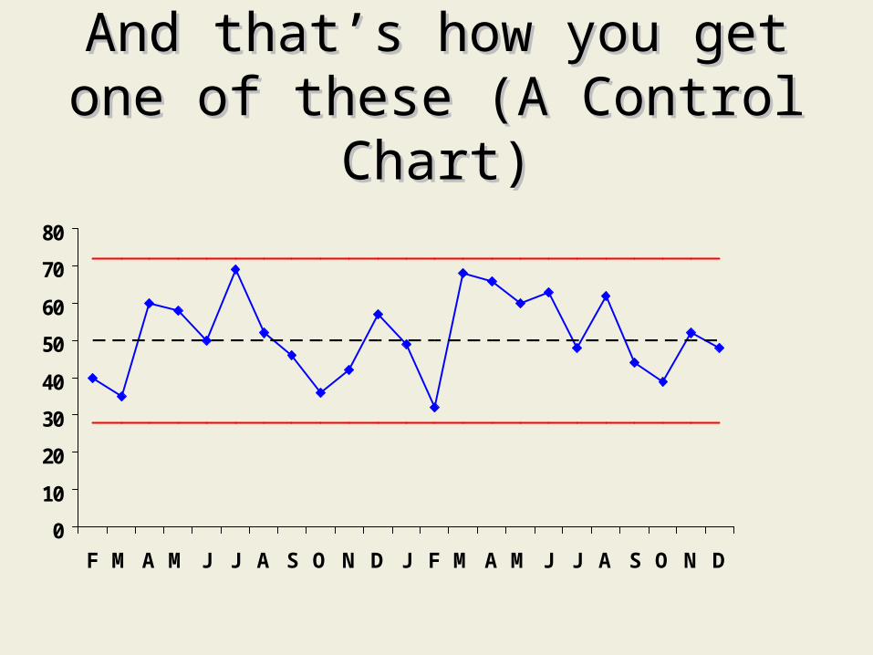
And that’s how you get one And that’s how you get one of these (A Control Chart)of these (A Control Chart)
0
10
20
30
40
50
60
70
80
F M A M J J A S O N D J F M A M J J A S O N D
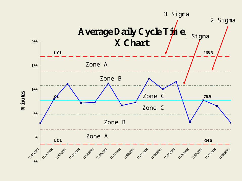
Average Daily Cycle TimeX Chart
168.3UCL
CL 76.9
LCL -14.5
-50
0
50
100
150
200
11/1
5/200
4
11/1
6/200
4
11/1
7/200
4
11/1
8/200
4
11/1
9/200
4
11/2
0/200
4
11/2
1/200
4
11/2
2/200
4
11/2
3/200
4
11/2
4/200
4
11/2
5/200
4
11/2
6/200
4
11/2
7/200
4
11/2
8/200
4
11/2
9/200
4
Min
utes
Zone A
Zone B
Zone C
Zone C
Zone B
Zone A
1 Sigma
2 Sigma3 Sigma
XX
X
X
X
X
X
X
X
LCL
UCL
MEAN
X
X
X
X
XX
X
X
X
X
LCL
UCL
MEAN
X
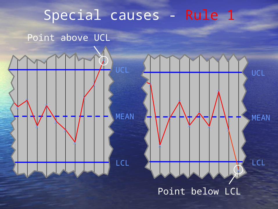
Point above UCL
Point below LCL
Special causes - Rule 1
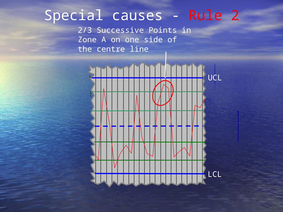
Special causes - Rule 22/3 Successive Points in Zone A on one side of the centre line
LCL
UCL
MEAN MEAN
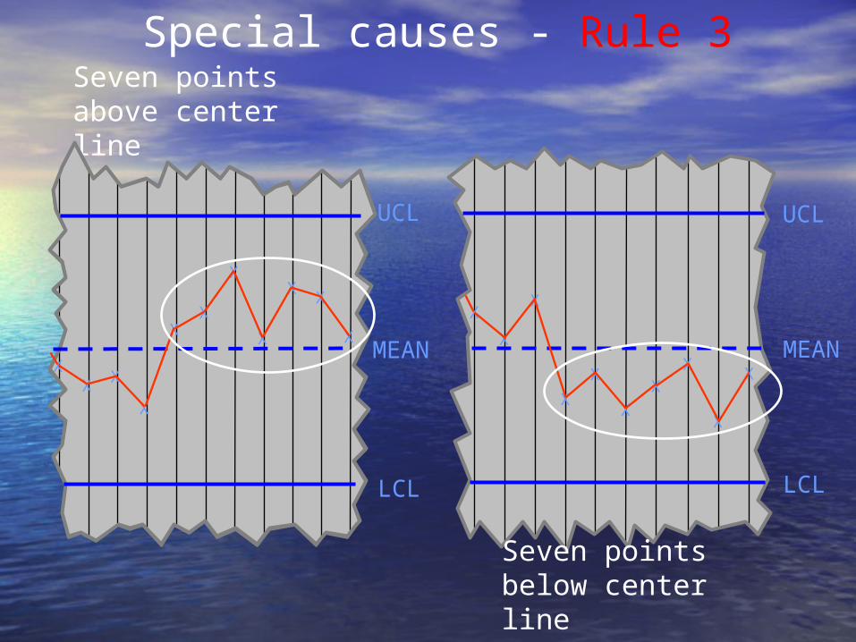
Seven points above center line
Special causes - Rule 3
LCL
UCL
LCL
UCL
XX
X
X
X X
X
XX
XX X
X
XX
X X
X
XX
X
Seven points below center line
MEAN MEAN
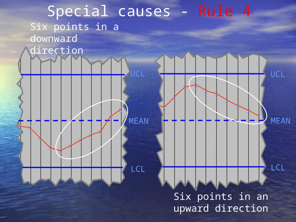
Six points in a downward direction
Special causes - Rule 4
LCL
UCL
LCL
UCL
XX
XX
X
XX
X
X X
X
XX X
XX
XX
X
X
X
Six points in an upward direction
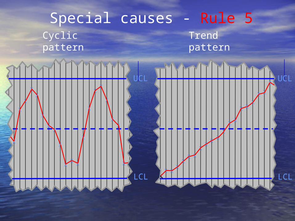
Special causes - Rule 5
X
X
X
X
X
X
XX X
X
X
X
X
X
X
X
X
X
X
X
Cyclic pattern
X
X X
XX
XX
X
X
X
X
X
X
X
X X
X
X
XLCL
UCL
LCL
UCL
Trend pattern

Which Type of SPC Chart Which Type of SPC Chart Should I Use?Should I Use?
• There are 30 or more types of SPC There are 30 or more types of SPC chartscharts
• Which one we choose depends on the Which one we choose depends on the question we’re askingquestion we’re asking
• These are available on computers – These are available on computers – no calculation neededno calculation needed
• Most important thing is to choose the Most important thing is to choose the right chart for the right question…..right chart for the right question…..

M e asure m e nt D ata C ount D ata
Subg r o up> 1
Subg r o up= 1
C o u n t #D e fe ct s
C o u n t# Un it s
" C o n s ta n t"O ppo rtu n ity
" Un e qu a l"O ppo rtu n ity
X B a r & SC h a rt
X M R (o r I )C h a rt
C -C h a rt U-C h a rt P-C h a rt
T yp e of D ata

Placeholder for Control Chart Placeholder for Control Chart DemoDemo
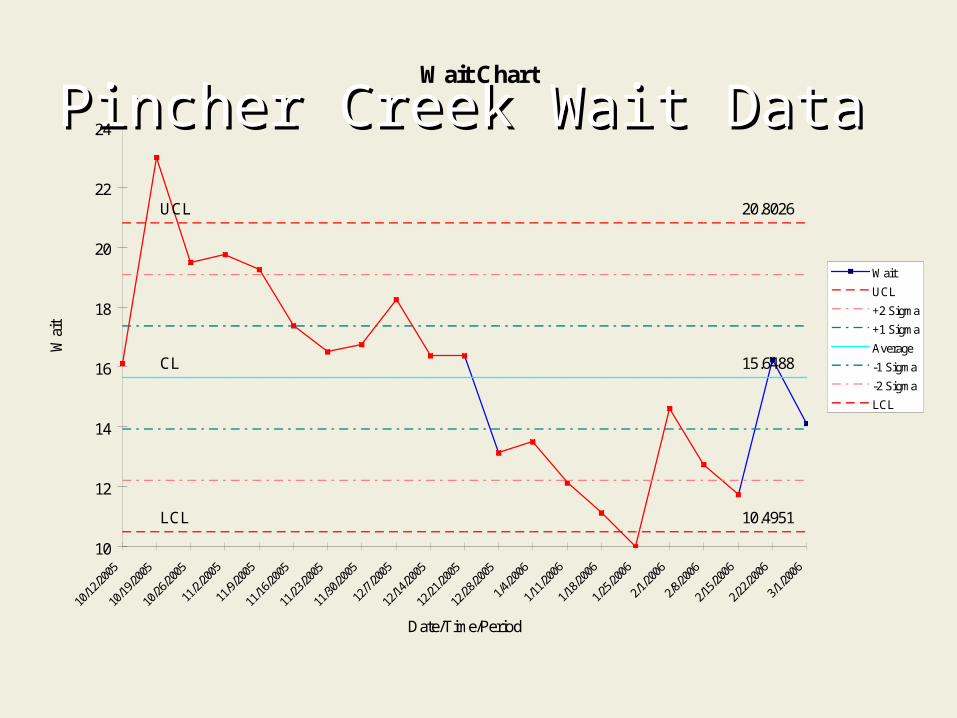
Pincher Creek Wait DataPincher Creek Wait DataWait Chart
20.8026UCL
CL 15.6488
LCL 10.4951
10
12
14
16
18
20
22
24
10/1
2/200
5
10/1
9/200
5
10/2
6/200
5
11/2
/2005
11/9
/2005
11/1
6/200
5
11/2
3/200
5
11/3
0/200
5
12/7
/2005
12/1
4/200
5
12/2
1/200
5
12/2
8/200
5
1/4/2
006
1/11
/2006
1/18
/2006
1/25
/2006
2/1/2
006
2/8/2
006
2/15
/2006
2/22
/2006
3/1/2
006
Date/Time/Period
Wai
t
Wait
UCL
+2 Sigma
+1 Sigma
Average
-1 Sigma
-2 Sigma
LCL

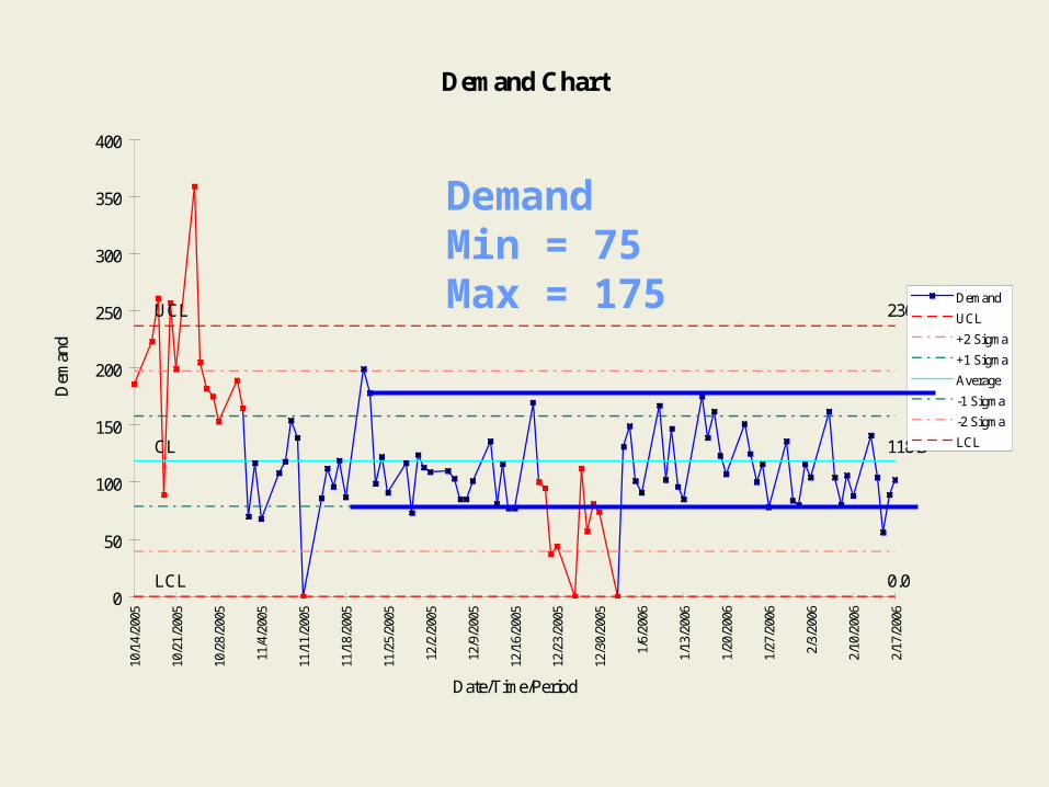
Demand Chart
236.9UCL
CL 118.5
LCL 0.00
50
100
150
200
250
300
350
40010
/14/
2005
10/2
1/20
05
10/2
8/20
05
11/4
/200
5
11/1
1/20
05
11/1
8/20
05
11/2
5/20
05
12/2
/200
5
12/9
/200
5
12/1
6/20
05
12/2
3/20
05
12/3
0/20
05
1/6/
2006
1/13
/200
6
1/20
/200
6
1/27
/200
6
2/3/
2006
2/10
/200
6
2/17
/200
6
Date/Time/Period
Dem
and
Demand
UCL
+2 Sigma
+1 Sigma
Average
-1 Sigma
-2 Sigma
LCL
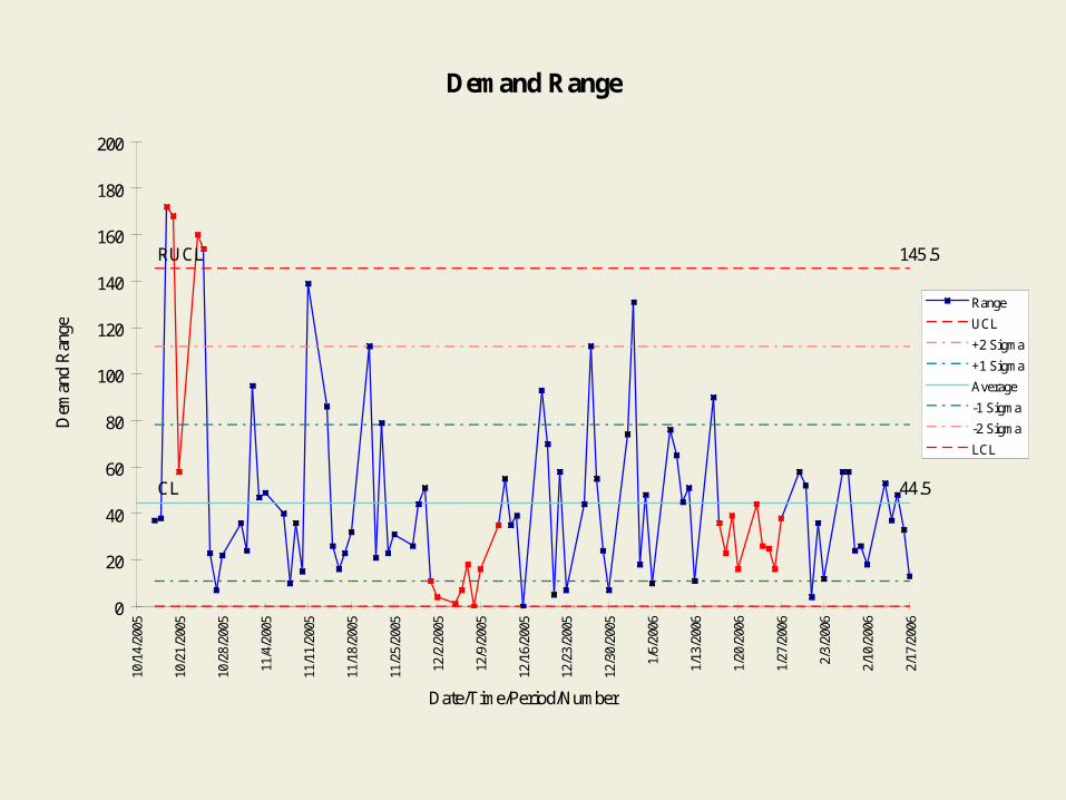
Demand Range
145.5RUCL
CL 44.5
0
20
40
60
80
100
120
140
160
180
20010
/14/
2005
10/2
1/20
05
10/2
8/20
05
11/4
/200
5
11/1
1/20
05
11/1
8/20
05
11/2
5/20
05
12/2
/200
5
12/9
/200
5
12/1
6/20
05
12/2
3/20
05
12/3
0/20
05
1/6/
2006
1/13
/200
6
1/20
/200
6
1/27
/200
6
2/3/
2006
2/10
/200
6
2/17
/200
6
Date/Time/Period/Number
Dem
and
Ran
ge
Range
UCL
+2 Sigma
+1 Sigma
Average
-1 Sigma
-2 Sigma
LCL
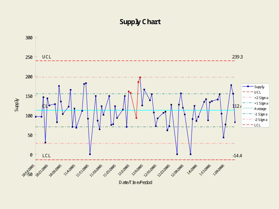
Supply Chart
239.3UCL
CL 112.4
LCL -14.4
-50
0
50
100
150
200
250
300
10/1
4/200
5
10/2
1/200
5
10/2
8/200
5
11/4
/2005
11/11
/2005
11/1
8/200
5
11/2
5/200
5
12/2
/2005
12/9
/2005
12/1
6/200
5
12/2
3/200
5
12/3
0/200
5
1/6/2
006
1/13
/2006
1/20
/2006
Date/Time/Period
Sup
ply
Supply
UCL
+2 Sigma
+1 Sigma
Average
-1 Sigma
-2 Sigma
LCL
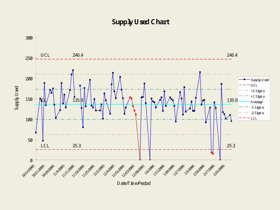
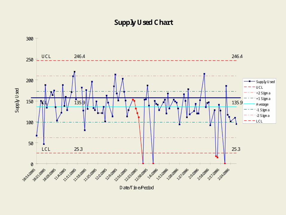
Supply Used Chart
246.4246.4UCL
CL 135.9135.9
LCL 25.325.3
0
50
100
150
200
250
300
10/1
4/200
5
10/2
1/200
5
10/2
8/200
5
11/4
/2005
11/11
/2005
11/1
8/200
5
11/2
5/200
5
12/2
/2005
12/9
/2005
12/1
6/200
5
12/2
3/200
5
12/3
0/200
5
1/6/2
006
1/13
/2006
1/20
/2006
1/27
/2006
2/3/2
006
2/10
/2006
2/17
/2006
2/24
/2006
Date/Time/Period
Sup
ply
Use
d
Supply Used
UCL
+2 Sigma
+1 Sigma
Average
-1 Sigma
-2 Sigma
LCL
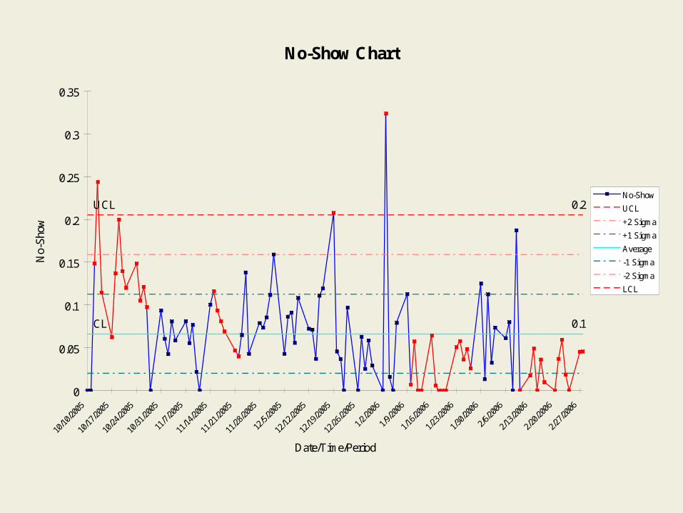
No-Show Chart
0.2UCL
CL 0.1
0
0.05
0.1
0.15
0.2
0.25
0.3
0.35
10/1
0/200
5
10/1
7/200
5
10/2
4/200
5
10/3
1/200
5
11/7
/2005
11/1
4/200
5
11/2
1/200
5
11/2
8/200
5
12/5
/2005
12/1
2/200
5
12/1
9/200
5
12/2
6/200
5
1/2/2
006
1/9/2
006
1/16
/2006
1/23
/2006
1/30
/2006
2/6/2
006
2/13
/2006
2/20
/2006
2/27
/2006
Date/Time/Period
No-
Sho
w
No-Show
UCL
+2 Sigma
+1 Sigma
Average
-1 Sigma
-2 Sigma
LCL

How Much S to meet D?How Much S to meet D?
• Common Cause VariationCommon Cause Variation
Demand Chart
236.9UCL
CL 118.5
LCL 0.00
50
100
150
200
250
300
350
40010
/14/
2005
10/2
1/20
05
10/2
8/20
05
11/4
/200
5
11/1
1/20
05
11/1
8/20
05
11/2
5/20
05
12/2
/200
5
12/9
/200
5
12/1
6/20
05
12/2
3/20
05
12/3
0/20
05
1/6/
2006
1/13
/200
6
1/20
/200
6
1/27
/200
6
2/3/
2006
2/10
/200
6
2/17
/200
6
Date/Time/Period
Dem
and
Demand
UCL
+2 Sigma
+1 Sigma
Average
-1 Sigma
-2 Sigma
LCL
Demand Min = 75Max = 175
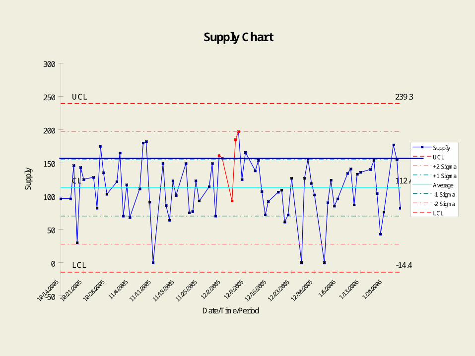
Supply Chart
239.3UCL
CL 112.4
LCL -14.4
-50
0
50
100
150
200
250
300
10/1
4/200
5
10/2
1/200
5
10/2
8/200
5
11/4
/2005
11/11
/2005
11/1
8/200
5
11/2
5/200
5
12/2
/2005
12/9
/2005
12/1
6/200
5
12/2
3/200
5
12/3
0/200
5
1/6/2
006
1/13
/2006
1/20
/2006
Date/Time/Period
Sup
ply
Supply
UCL
+2 Sigma
+1 Sigma
Average
-1 Sigma
-2 Sigma
LCL
Supply Used Chart
246.4246.4UCL
CL 135.9135.9
LCL 25.325.3
0
50
100
150
200
250
300
10/1
4/200
5
10/2
1/200
5
10/2
8/200
5
11/4
/2005
11/11
/2005
11/1
8/200
5
11/2
5/200
5
12/2
/2005
12/9
/2005
12/1
6/200
5
12/2
3/200
5
12/3
0/200
5
1/6/2
006
1/13
/2006
1/20
/2006
1/27
/2006
2/3/2
006
2/10
/2006
2/17
/2006
2/24
/2006
Date/Time/Period
Sup
ply
Use
d
Supply Used
UCL
+2 Sigma
+1 Sigma
Average
-1 Sigma
-2 Sigma
LCL
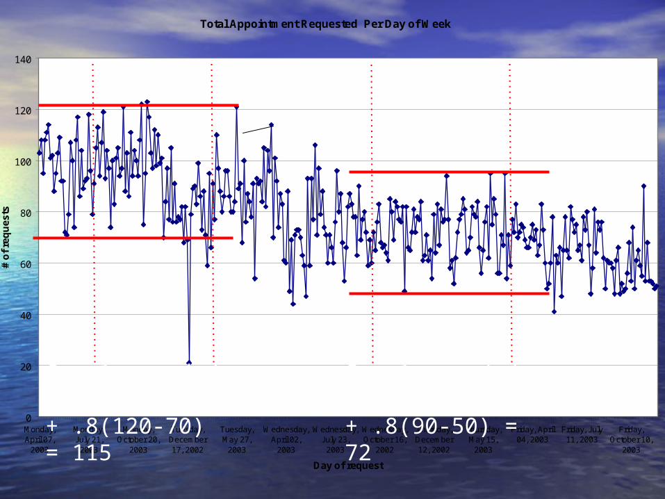
Total Appointment Requested Per Day of Week
0
20
40
60
80
100
120
140
Monday,April 07,
2003
Monday,July 21,
2003
Monday,October 20,
2003
Tuesday,December17, 2002
Tuesday,May 27,
2003
Wednesday,April 02,
2003
Wednesday,July 23,
2003
Wednesday,October 16,
2002
Thursday,December12, 2002
Thursday,May 15,
2003
Friday, April04, 2003
Friday, July11, 2003
Friday,October 10,
2003
Day of request
# o
f re
qu
ests
Monday Tuesday Wednesday Thursday Friday
Supply needed is 40 + .8(90-50) = 72
Supply needed is 70 + .8(120-70) = 115
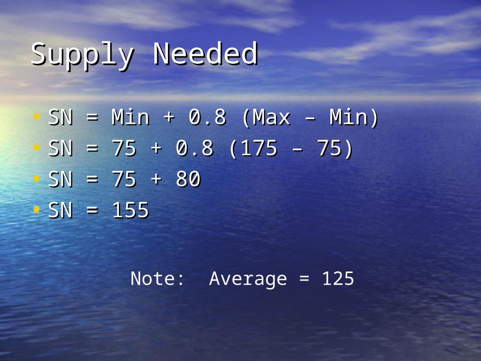
Supply NeededSupply Needed
• SN = Min + 0.8 (Max – Min)SN = Min + 0.8 (Max – Min)
• SN = 75 + 0.8 (175 – 75)SN = 75 + 0.8 (175 – 75)
• SN = 75 + 80SN = 75 + 80
• SN = 155SN = 155
Note: Average = 125
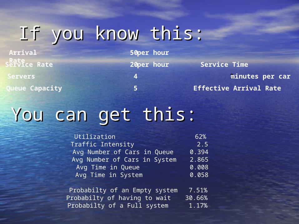
If you know this:If you know this:
You can get this:You can get this:
ArrivalRate
50 per hour
Service Rate 20 per hour Service Time
Servers 4 3 minutes per car
Queue Capacity 5 Effective Arrival Rate
Utilization 62%Traffic Intensity 2.5Avg Number of Cars in Queue 0.394Avg Number of Cars in System 2.865Avg Time in Queue 0.008Avg Time in System 0.058
Probabilty of an Empty system 7.51%Probabilty of having to wait 30.66%Probabilty of a Full system 1.17%

Queuing Allows Calculation Queuing Allows Calculation of:of:• Number of servers needed under Number of servers needed under
various conditions (supply)various conditions (supply)
• Amount of wait resulting from a Amount of wait resulting from a systemsystem
………………..As long as the arrival rate is ..As long as the arrival rate is even, there are no unusual events, even, there are no unusual events, and the system is simpleand the system is simple

Computer Computer Modeling/SimulationModeling/Simulation
• Applications that mimic the behavior Applications that mimic the behavior of real systems on a computerof real systems on a computer
• Allows “playing” with the systemAllows “playing” with the system
• Allows asking “what if” questionsAllows asking “what if” questions
• Can see results of changesCan see results of changes
Top Related