


Languages
Pages
Legal

0 'SIDESRUTIIAD-A259 236
.~. 31 - 3,
I-MIM Im a FMIMIGL~r0
-3-SWMP :
A0ff
bOTI
U .::. 2=7:99
U S Arm Cop fEnier
.5..gor, G 2.0 314-0 00
Destroy this report when no longer needed. Do not returnit to the originator.
The findings in this report are not to be construed as an officialDepartment of the Army position unless so designated
by other authorized documents.
The contents of this report are not to be used foradvertising, publication, or promotional purposes.
Citation of trade names does not constitute anofficial endorsement or approval of the use of
such commercial products.
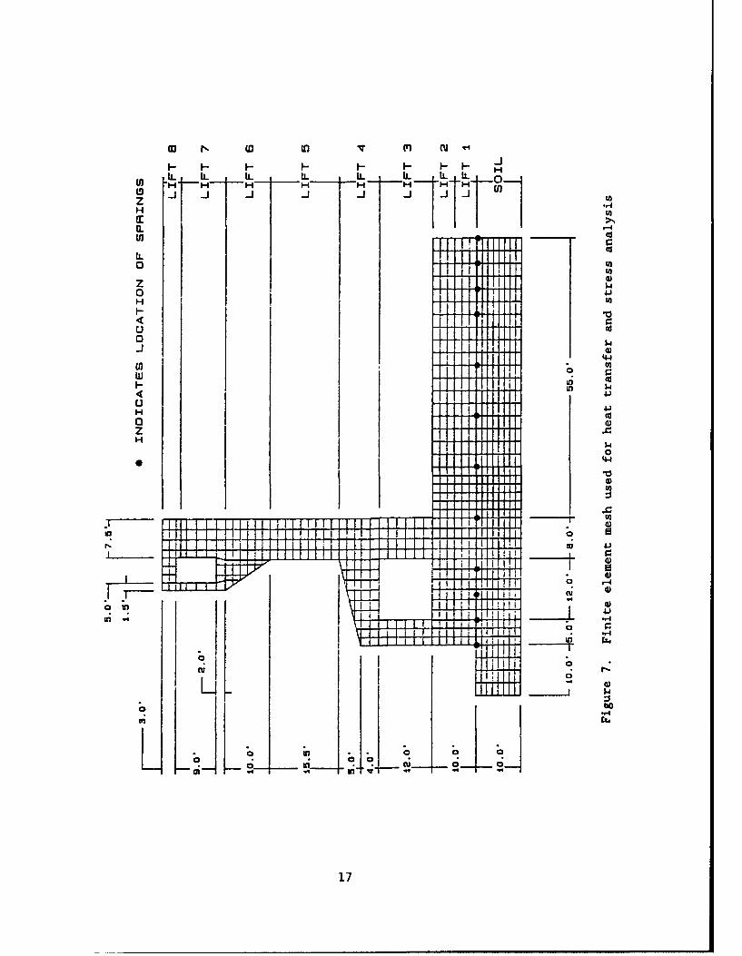
Form ApprovedREPORT DOCUMENTATION PAGE OMB No. 0704-0188
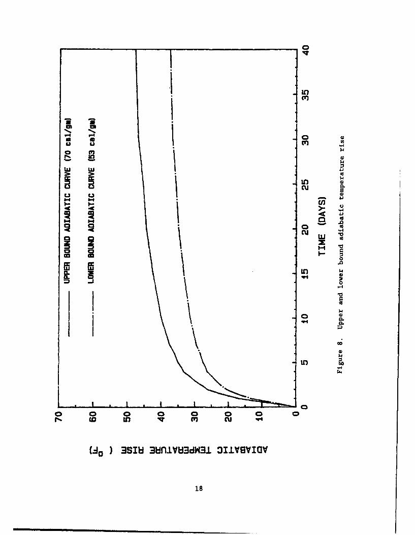
Public reporting burden for this collection of information is estimated to average 1 hour per response, including the time for reviewing instructions, searching existing data sources.gathering and maintaining the data needed. and completing and reviewing the collection of Irformation. Send comments regarding this burden estimate or any other aspect of thiscollection of information, including suggestions for reducing this burden. to Washington Headquarters Services, Directorate for information Operations and Reports, 1215 JeffersonDavis Highway, Suite 1204. Arlington, VA 22202-4302. and to the Office of Management and Budget. Paperwork Reduction Project (0704-0188), Washington, DC 20503.
1. AGENCY USE ONLY (Leave blank) 2. REPORT DATE 3. REPORT TYPE AND DATES COVEREDSeptember 1992 Final report
4iTITLE AND SUBTITLE S. FUNDING NUMBERSvaluatlon of-Thermal and Incremental Construction
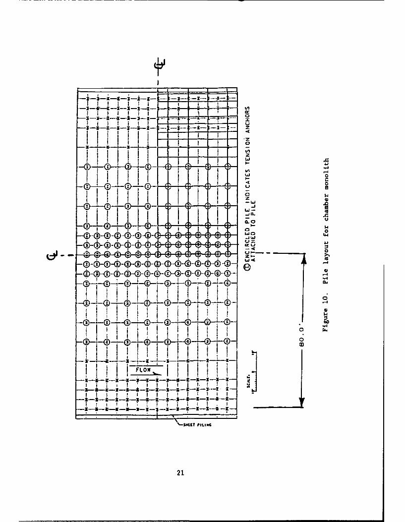
Effects for Monoliths AL-3 and AL-5 of the Melvin DACW39-87-K-0065Price Locks and Dams
6. AUTHOR(S)
Kevin Z. TrumanDavid J. PetruskaAbdelkader Ferhi
7. PERFORMING ORGANIZATION NAME(S) AND ADDRESS(ES) 8. PERFORMING ORGANIZATIONREPORT NUMBER
Department of Civil Engineering Contract ReportWashington University ITL-92-3St. Louis, Missouri
9. SPONSORING/MONITORING AGENCY NAME(S) AND ADDRESS(ES) 10. SPONSORING/MONITORINGUS Army Corps of Engineers AGENCY REPORT NUMBER
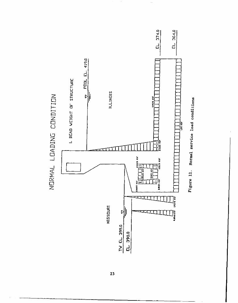
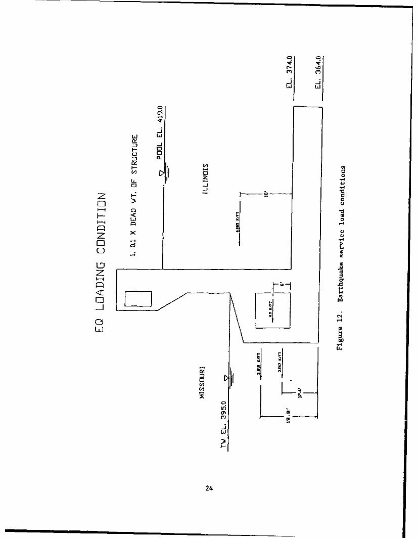
Washington, DC 20314-1000 andUSAE Waterways Experiment Station, InformationTechnology Laboratory, 3909 Halls Ferry Road,Vicksburg, MS 39180-6199
11. SUPPLEMENTARY NOTES
Available from National Technical Information Service, 5285 Port Royal Road,
Springfield, VA 22161
12a. DISTRIBUTION /AVAILABILITY STATEMENT 12b. DISTRIBUTION CODE
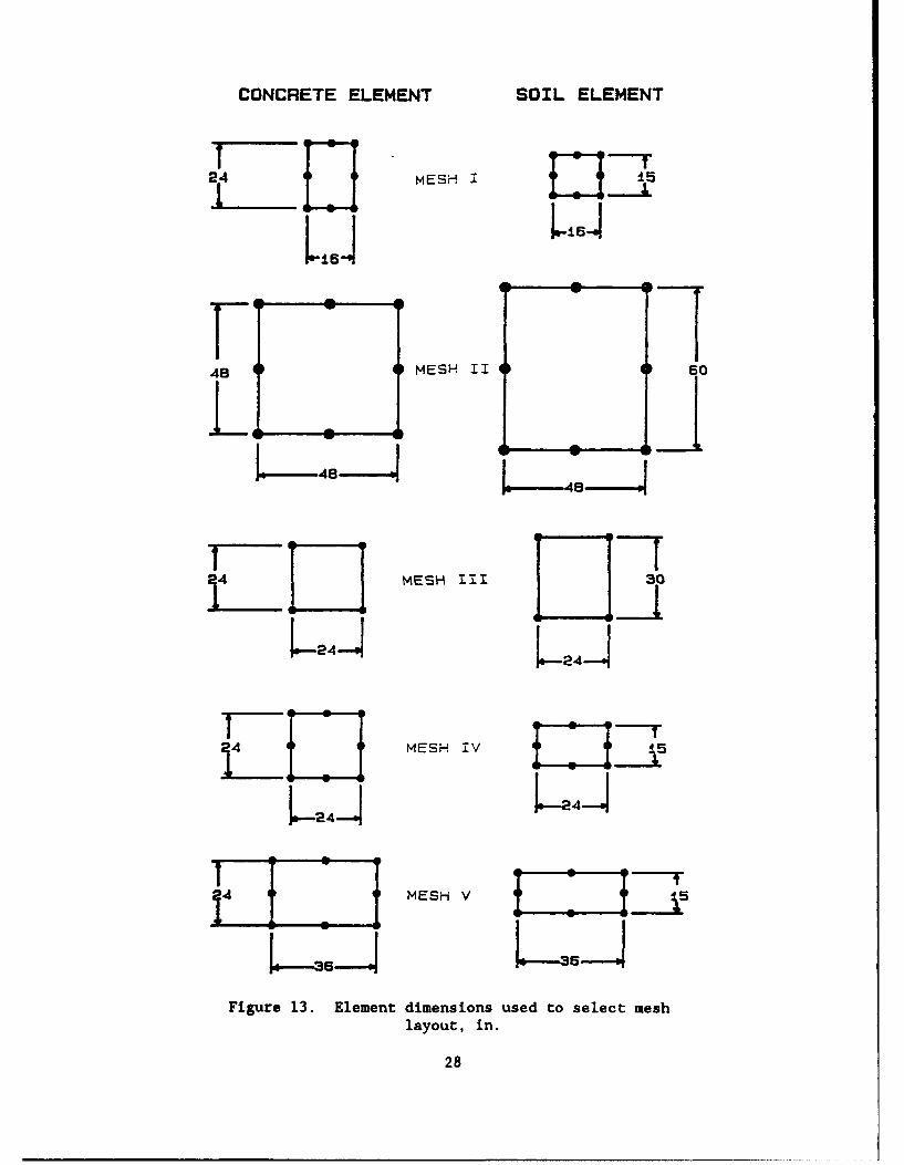
Approved for public release; distribution is unlimited
13. ABSTRACT (Maximum 200 words)
Two monoliths, a gate monolith and a chamber monolith, from the auxiliarylock at Melvin Price Locks and Dam near Alton, Illinois, are used to explore andevaluate the effects of creep, shrinkage, thermal loads, and constructionsequence on massive concrete structures. The material and structural modelling,analysis procedures and software, and results are thoroughly discussed. Thenonlinear material subroutines used to model aging modulus, autogenous shrink-age, creep, and smeared crack capabilities are described and discussed withregards to their use in modelling the structure and analyzing structural behav-ior. These parameters were used to perform a thorough parametric evaluation oftheir effects on massive concrete structures. The structural models for eachmonolith and its pile/soil foundation for both the thermal and mechanical analy-ses are provided. A detailed discussion regarding incremental construction forsimulating construction is presented. The incremental analysis procedure was
(Continued)
14. SUBJECT TERMS 15. NUMBER OF PAGESAging modulus Parametric 389Creep Shrinkage 16. PRICE CODEIncremental construction
17. SECURITY CLASSIFICATION 18. SECURITY CLASSIFICATION 19. SECURITY CLASSIFICATION 20. LIMITATION OF ABSTRACTOF REPORT OF THIS PAGE OF ABSTRACT
UNCLASSIFIED UNCLASSIFIED I I _I
NSN 7540-01-280-5500 Standard Form 298 (Rev 2-89)Prescribed by ANSI Stdi 29-IS298-102
13. ABSTRACT (Concluded).
that the lift heights in the gate monolith could be extended in various regionsresulting in a minimum savings of $720,000. Each aspect of the modelling andthe results are thoroughly discussed and documented through the use of time his-tory plots of critical location temperatures, stresses and strains.
PREFACE
The analyses and research described in this report were conducted by the
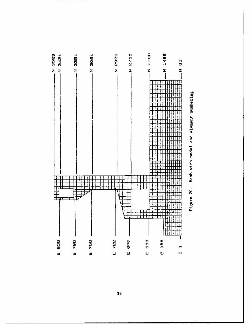
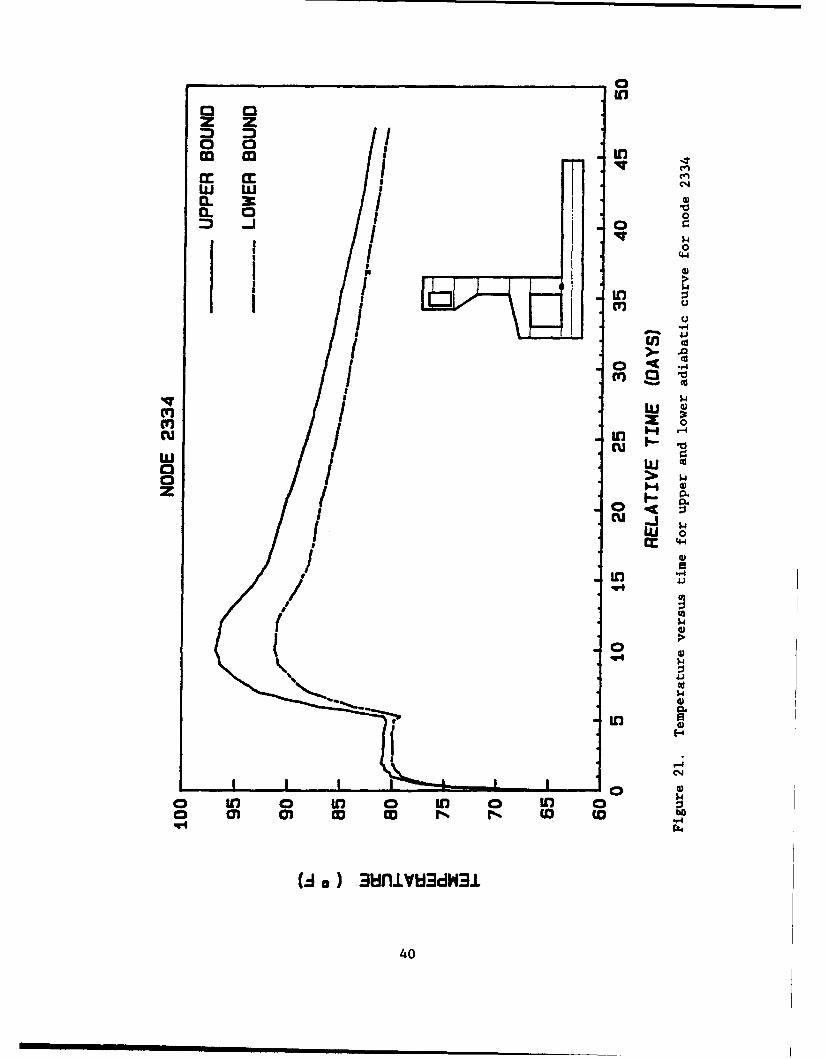
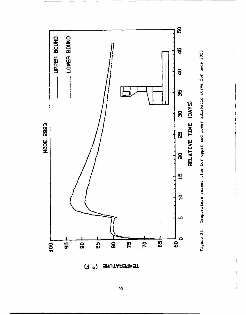
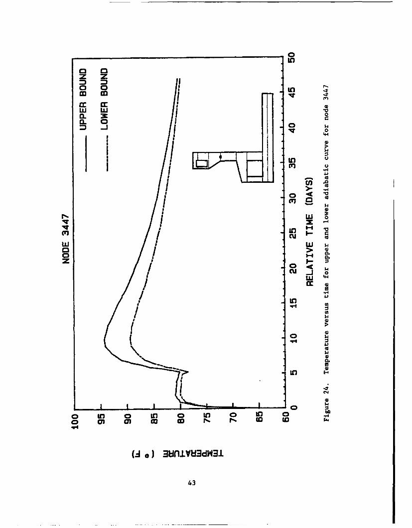
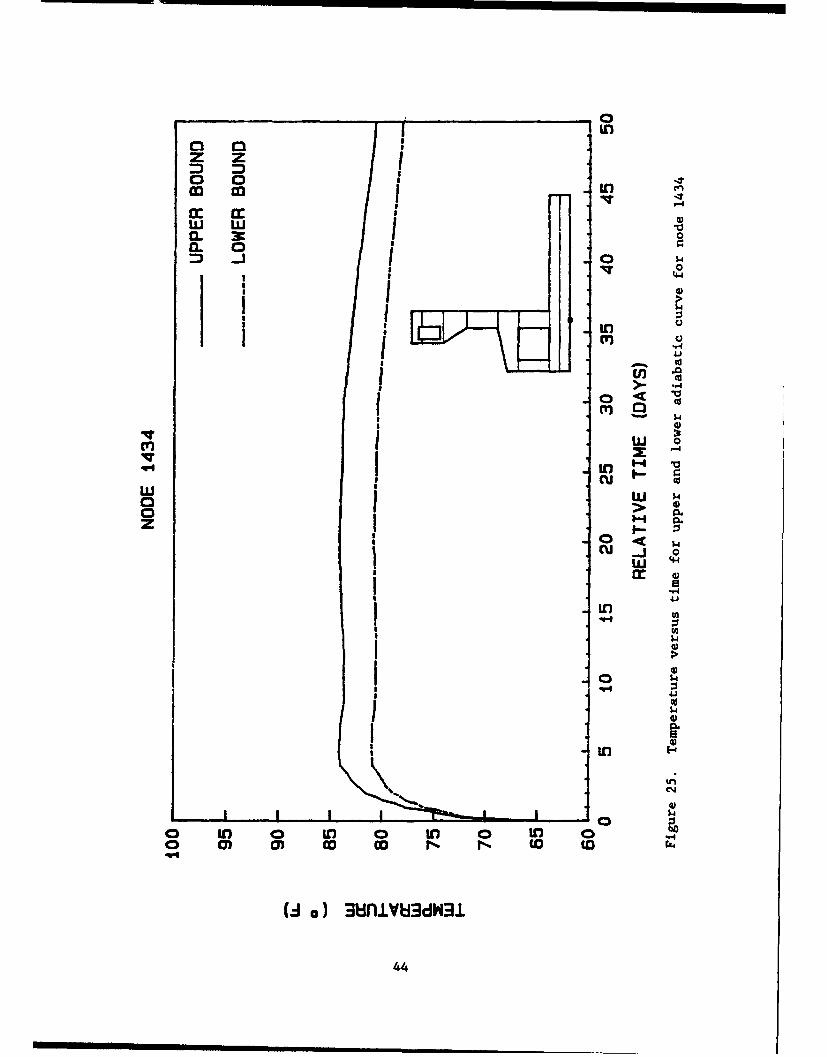
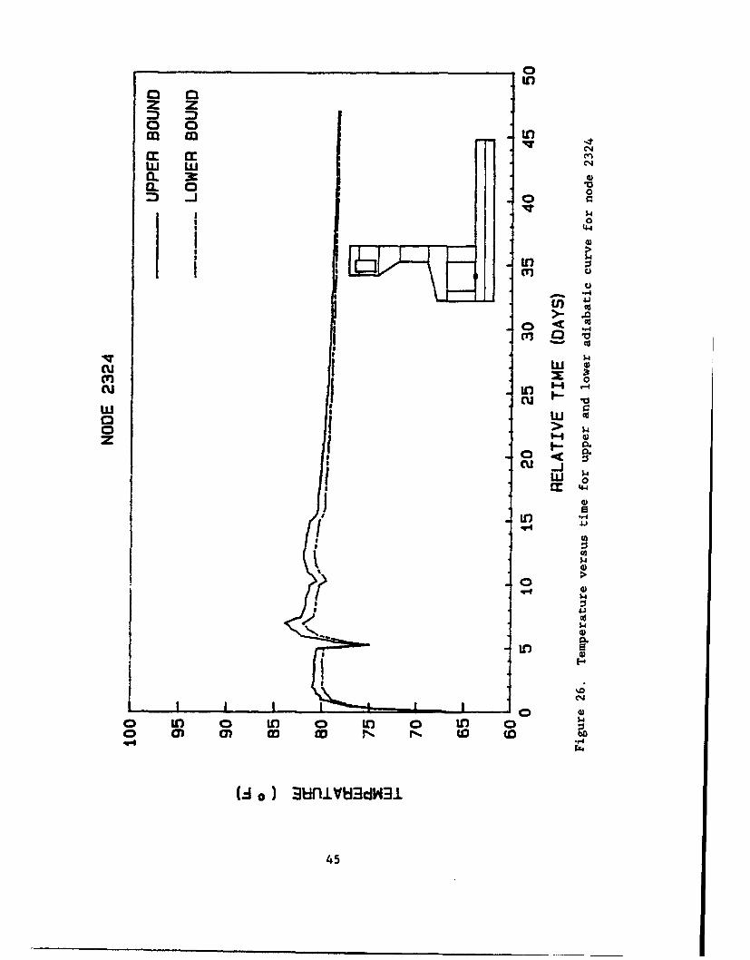
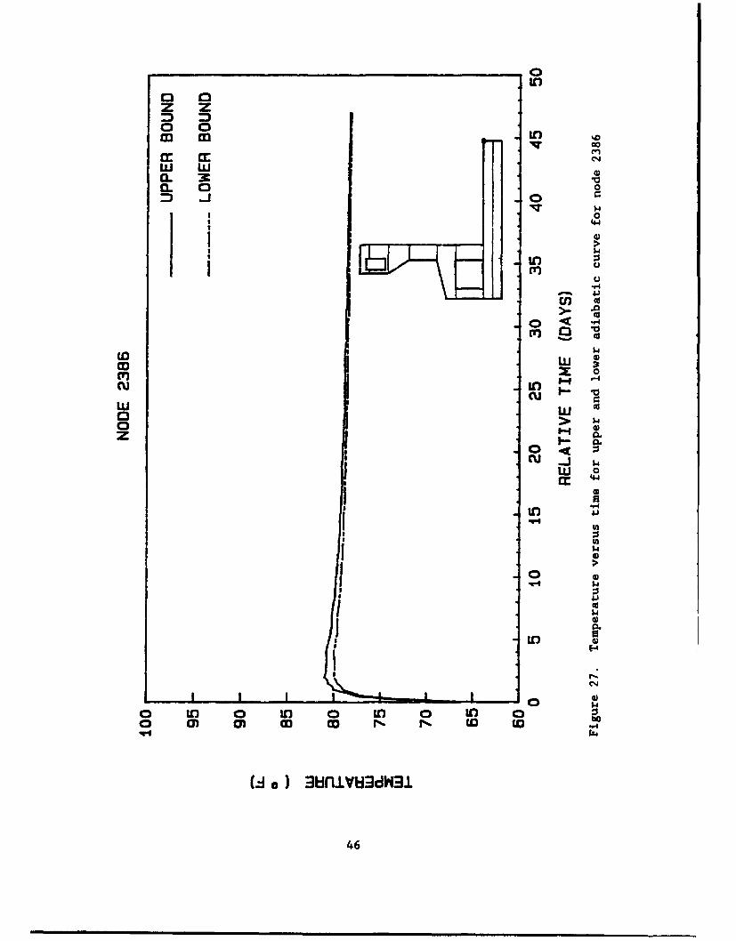
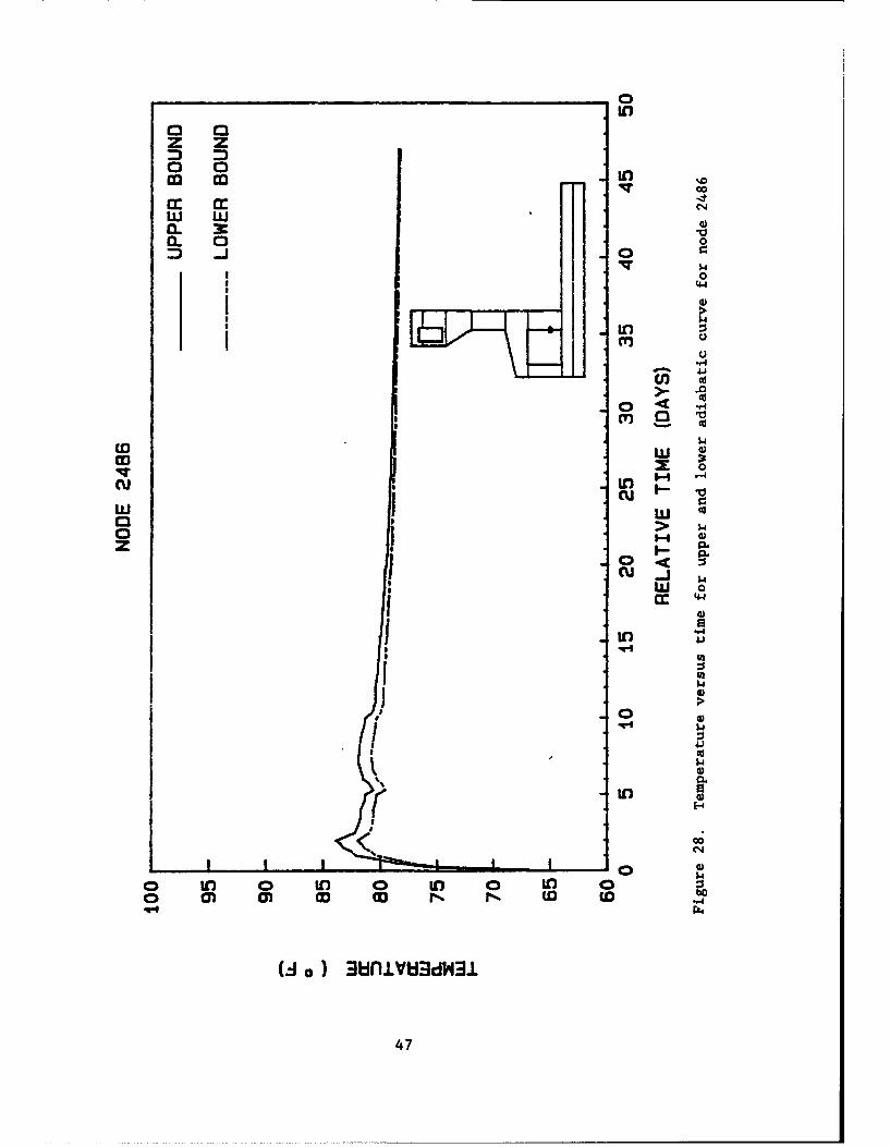
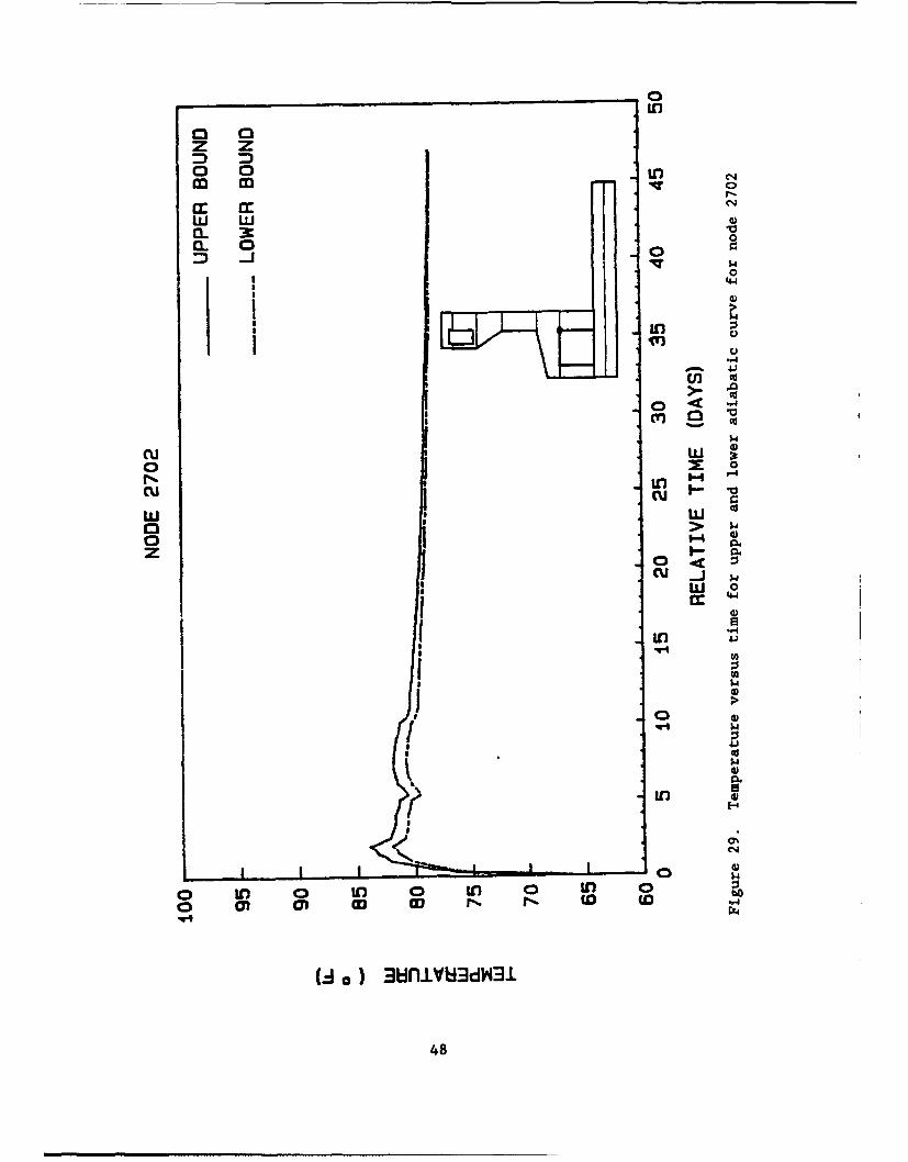
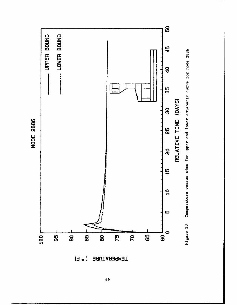
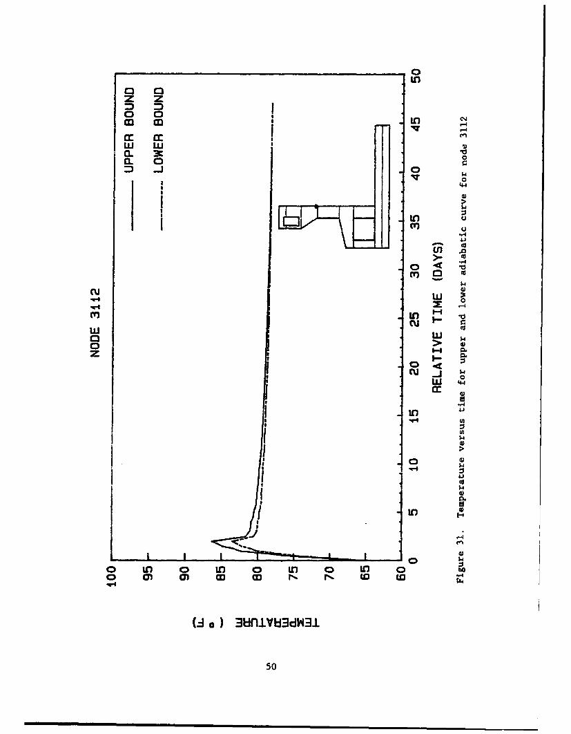
Department of Civil Engineering, College of Engineering, Washington Univer-
sity, in St. Louis, Missouri, for Headquarters, US Army Corps of Engineers.
The study was performed under Contract No. DACW39-87-K-0065 to the Information
Technology Laboratory (ITL), US Army Engineer Waterways Experiment Station
(WES). This study was conducted as part of the Phase II Thermal Studies
funded through the Melvin Price Locks and Dam project. The Technical Monitor
for the Phase II Thermal Studies was Mr. Barry Fehl, Structural Engineer in
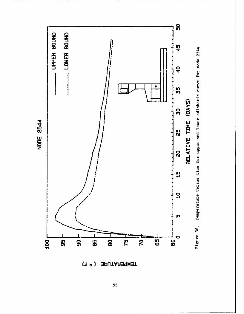
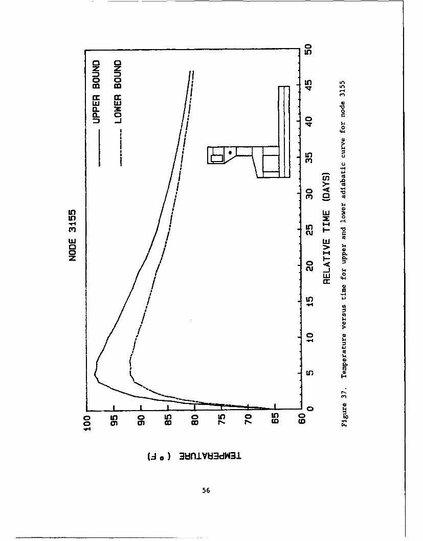
the Structural Section of the St. Louis District.
This report was prepared by Dr. Kevin Z. Truman, Mr. David J. Petruska,
and Mr. Abdelkader Fehri. Funds for publication of the report were provided
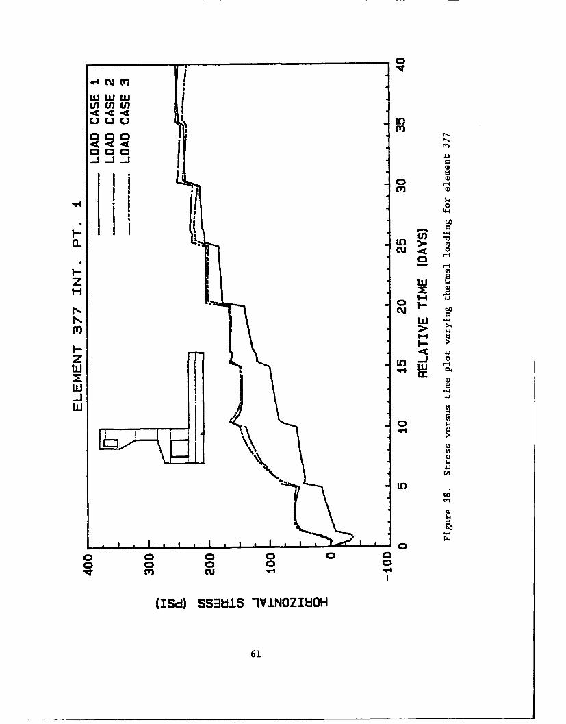
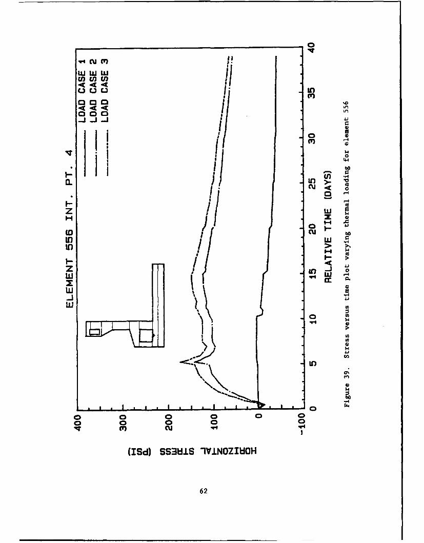
from those available for the Computer-Aided Structural Engineering (CASE)
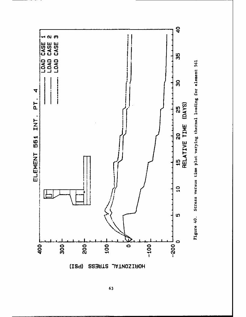
Project managed by ITL. Dr. N. Radhakrishnan, Director, ITL, is Project Man-
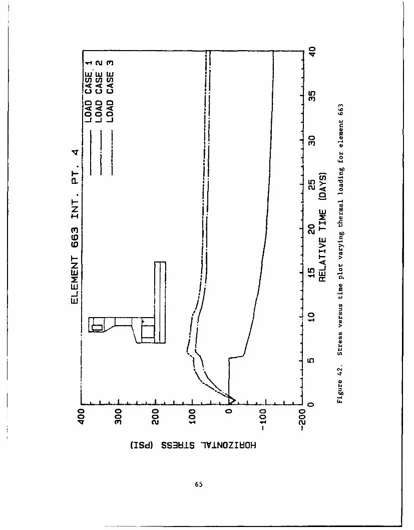
ager for the CASE Project.
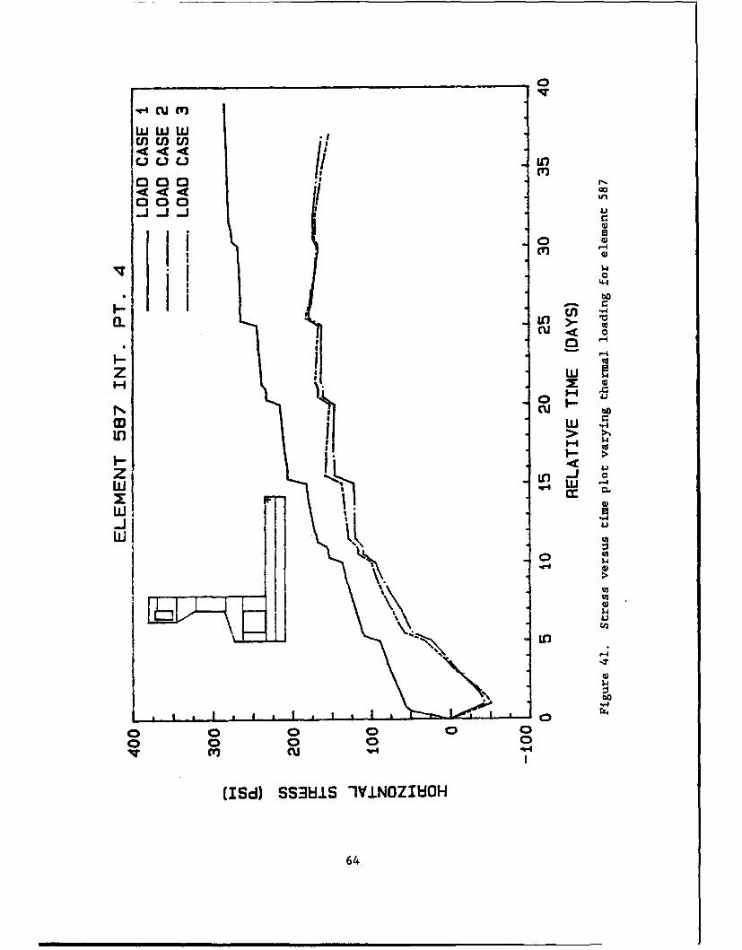
At the time of publication of this report, Director of WES was
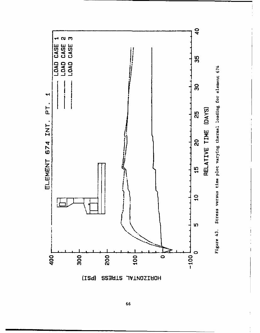
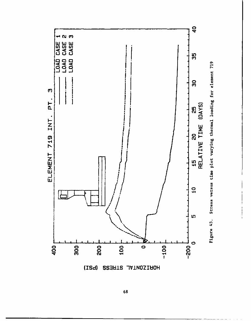
Dr. Robert W. Whalin. Commander and Deputy Director was COL Leonard G.
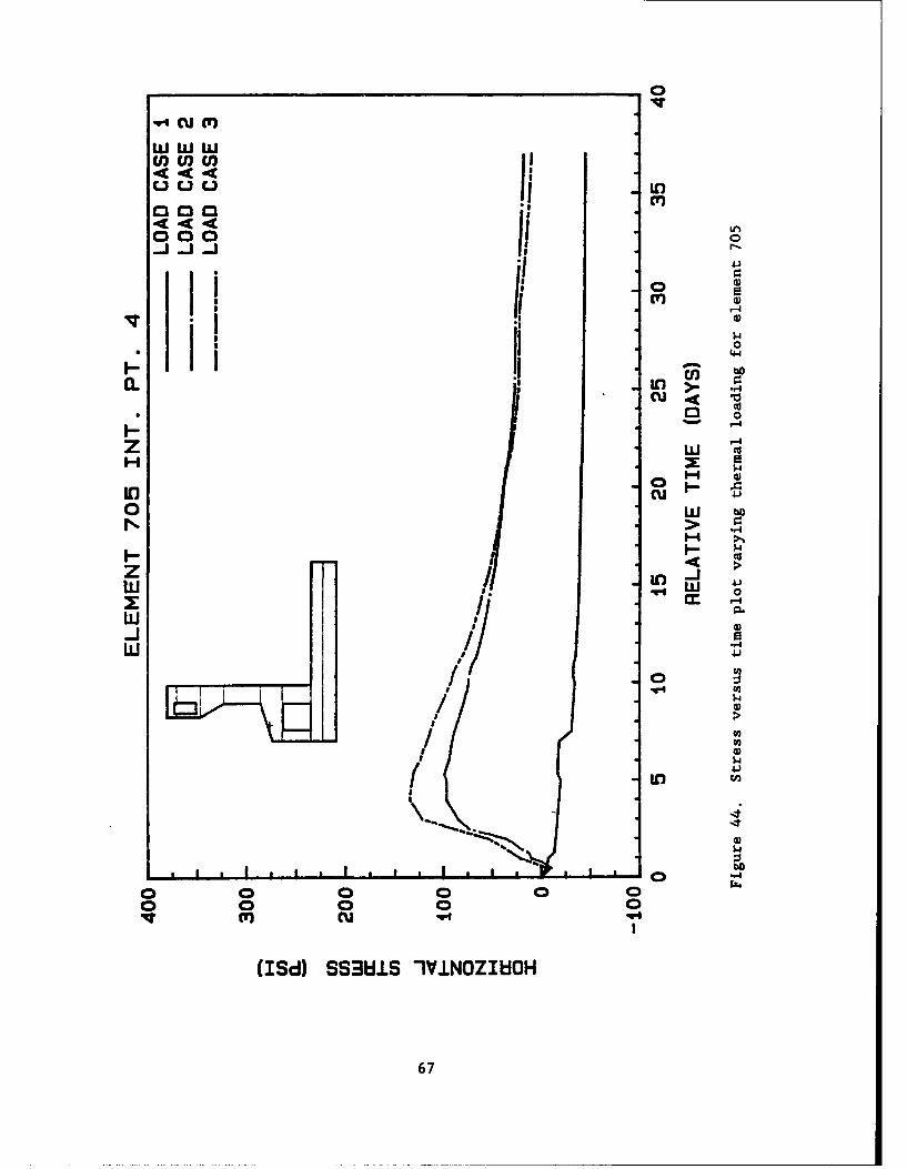
Hassell, EN.
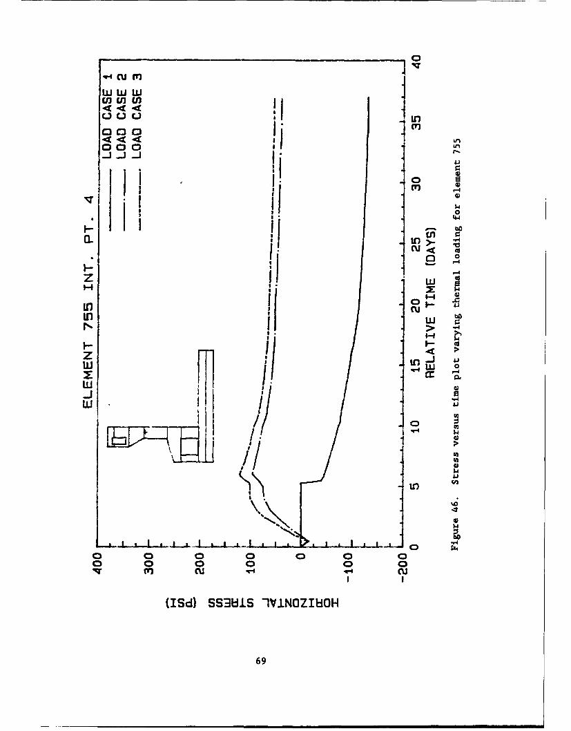
Accesioa For
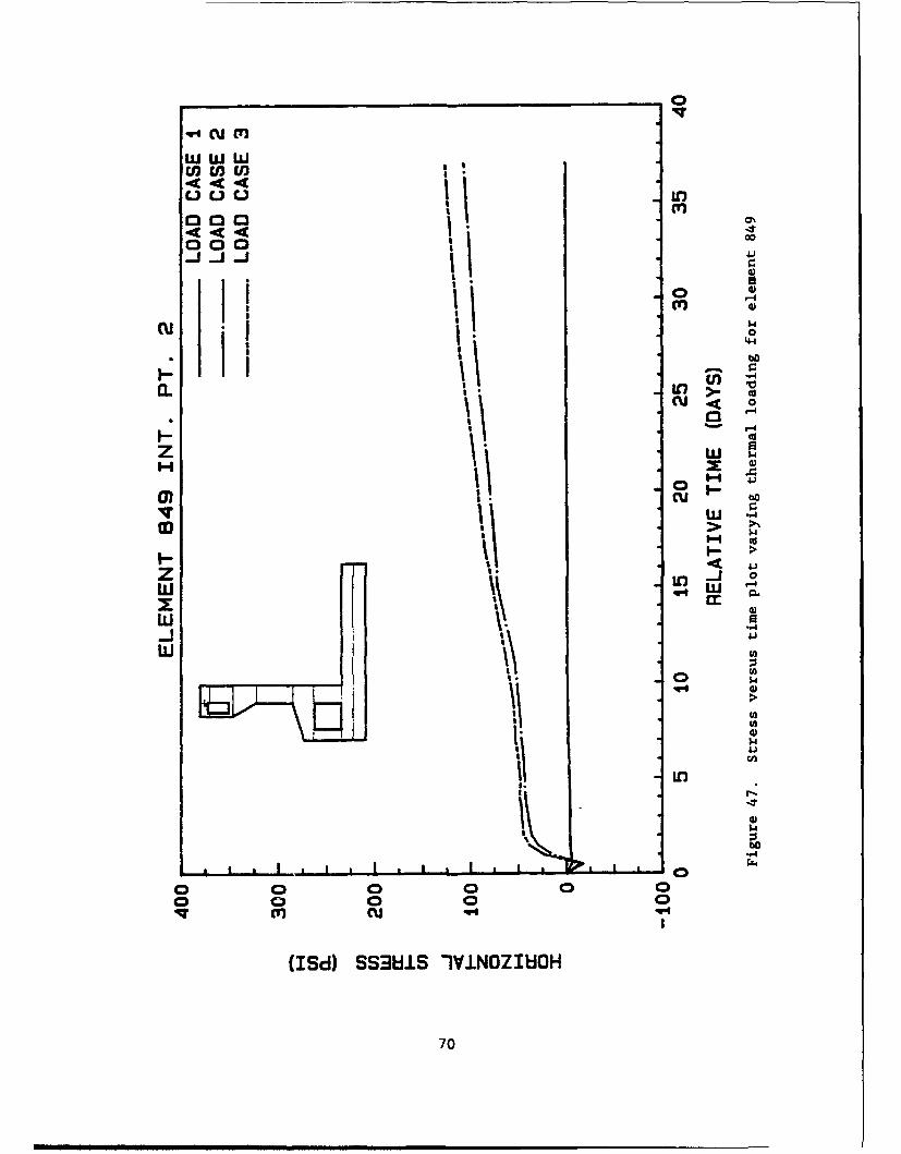
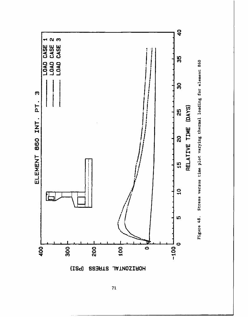
NTIS CRA&IDTIC IAS
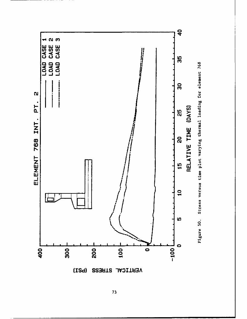
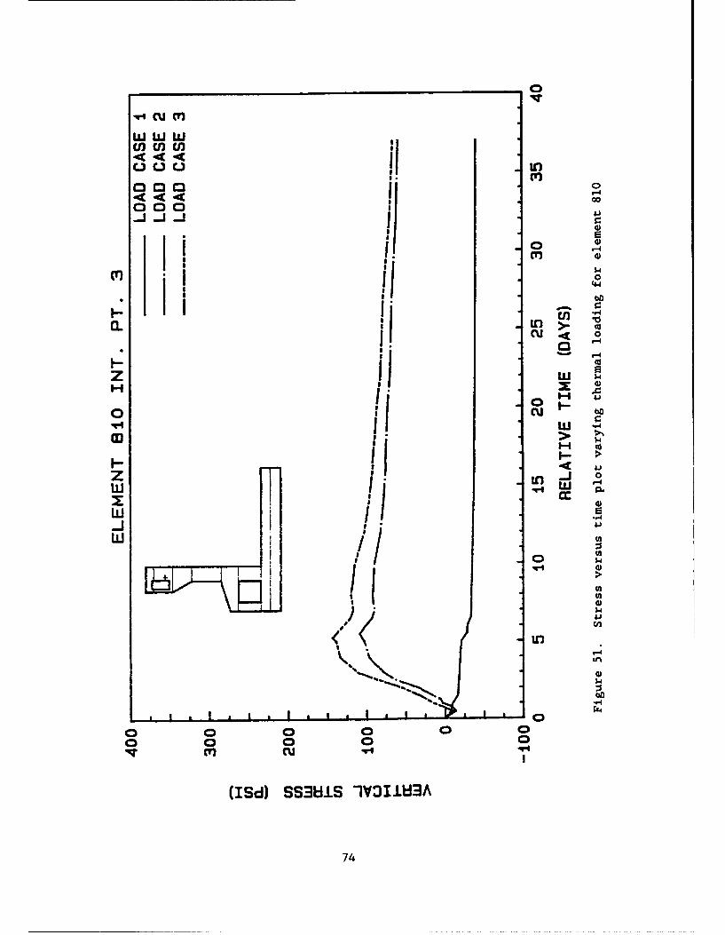
-dU, L1olceJuIstfication
a.. . . . . ......._............. .......... ......
By............................ ....................DiAt ibutioi o
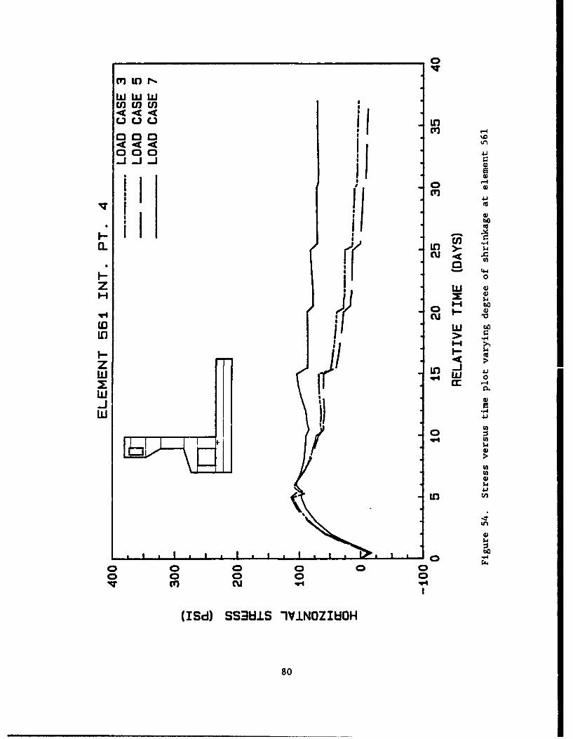
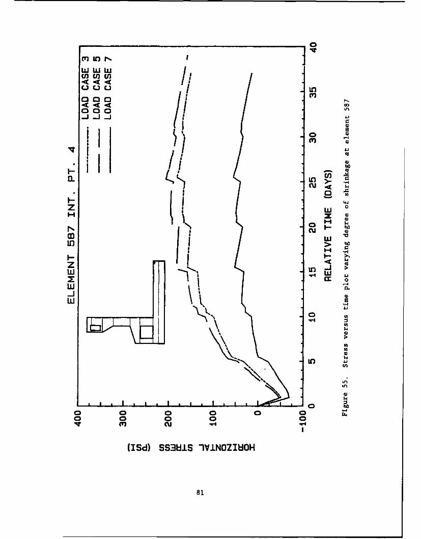
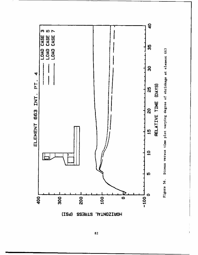
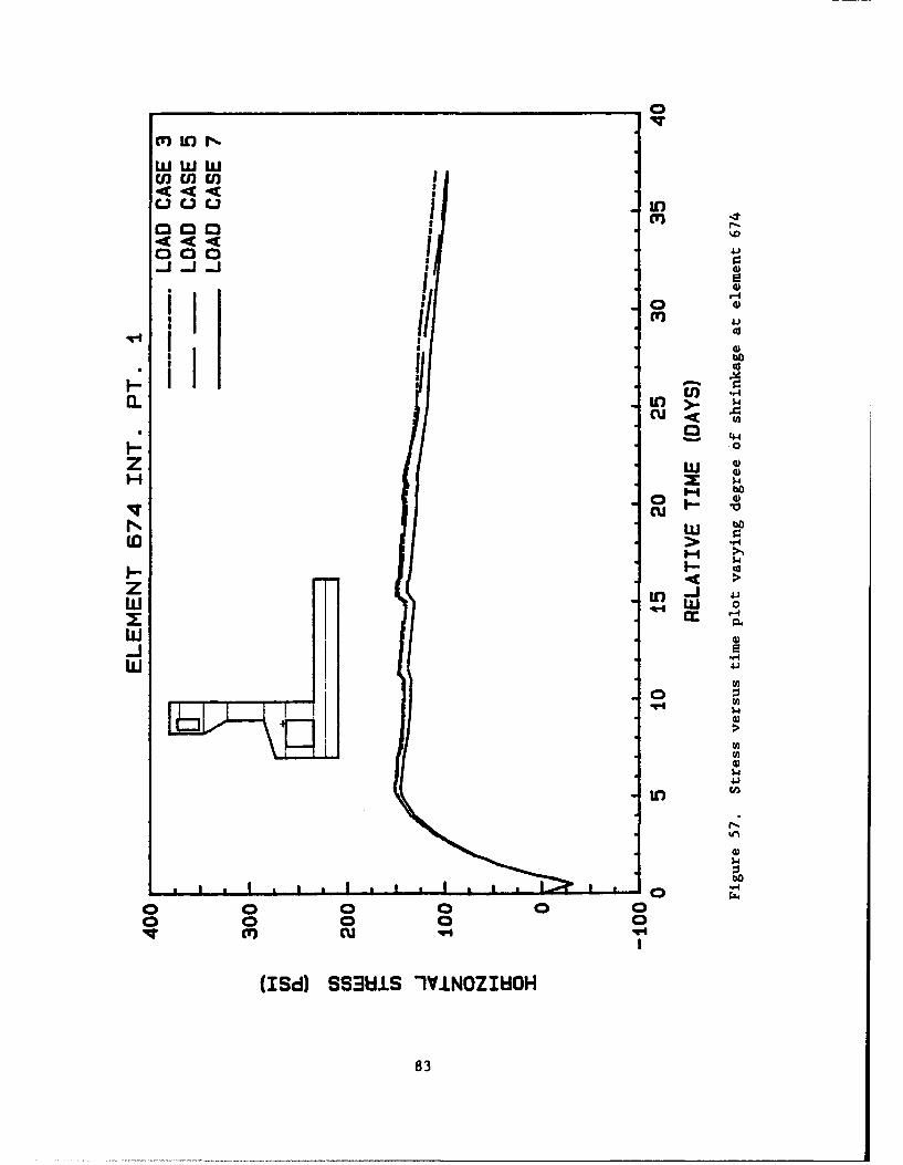
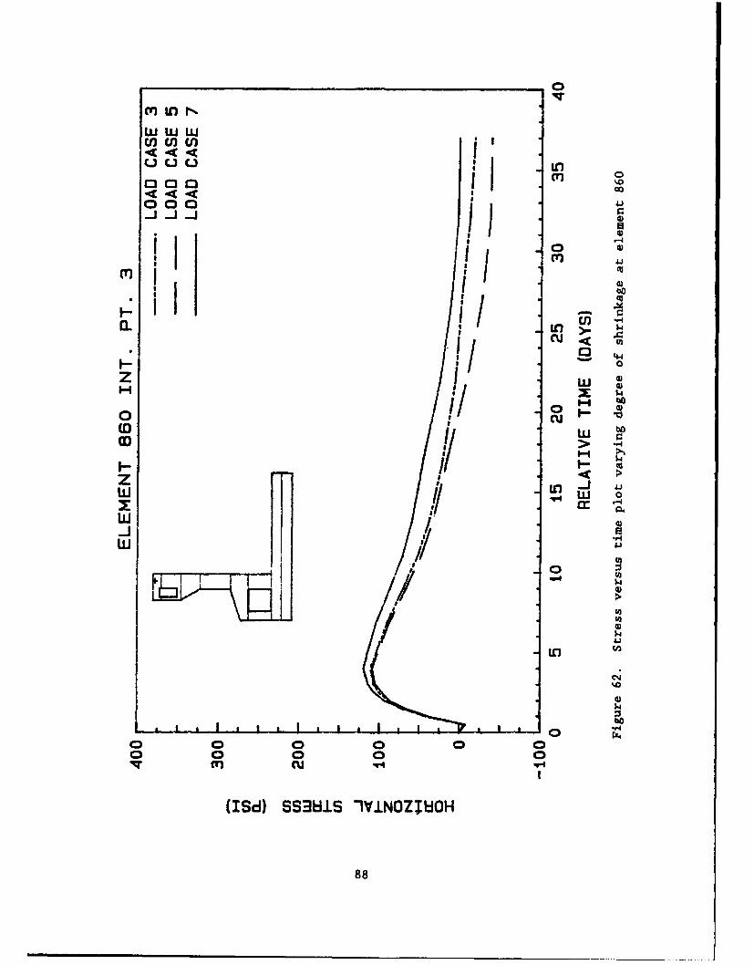
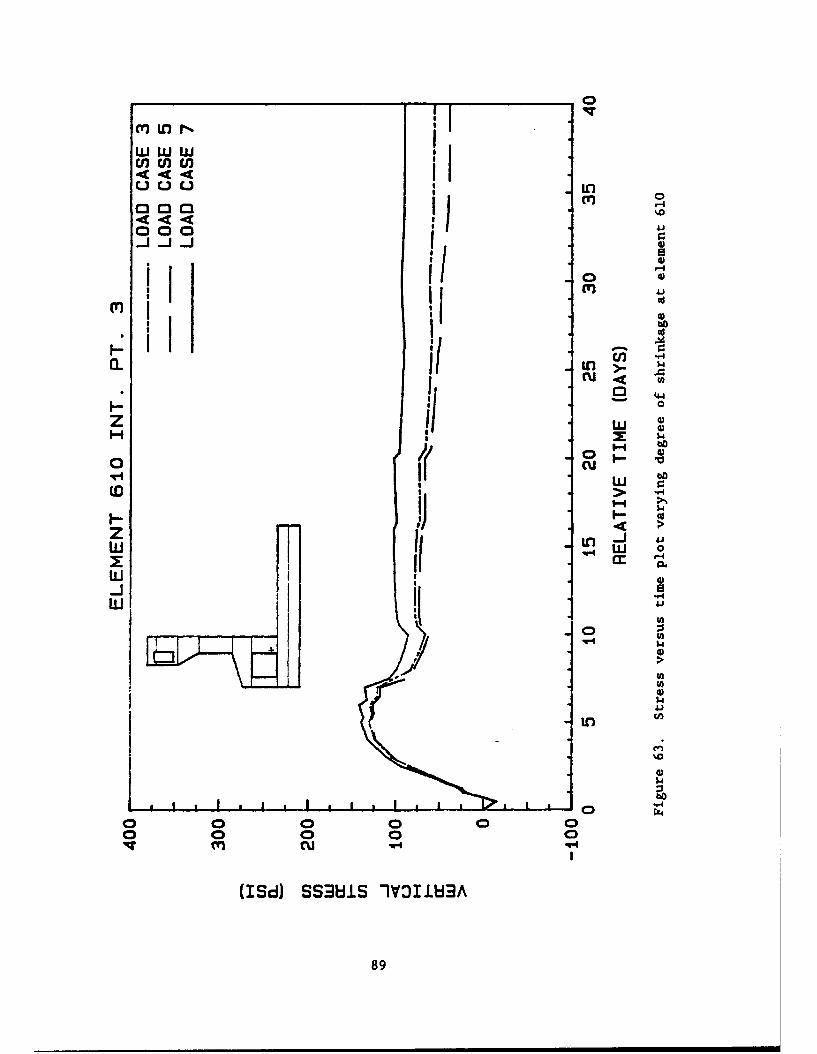
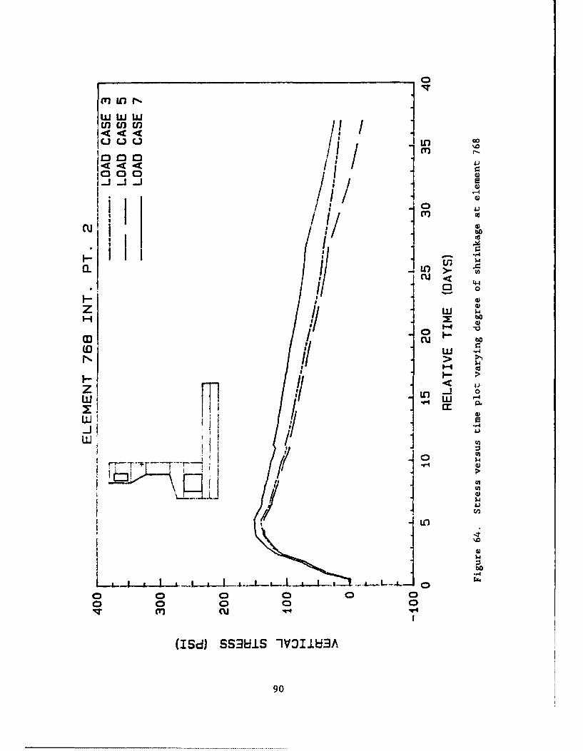
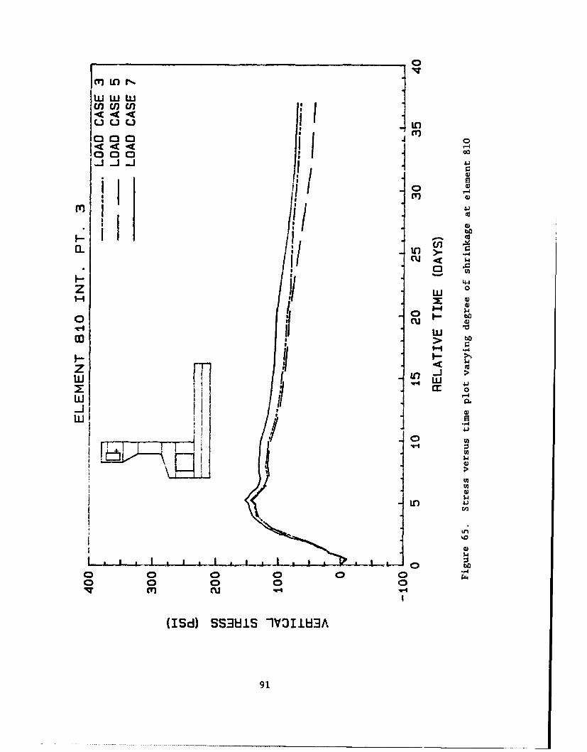
Availabnity CodesAvail arwjjor
Dist Spca
L I
CONTENTS
Page
PREFACE .......................... ................................ 1
CONVERSION FACTORS, NON-SI TO SI (METRIC) UNITSOF MEASUREMENT ....................... ........................... 4
PART I: INTRODUCTION ............ .......................... 5
Introduction ....................... .......................... 5Objective and Scope ................... ....................... 10
PART II: MODELLING AND MATERIAL PROPERTIES FOR MONOLITH AL-5 . . . . 12
Introduction .................. .......................... ... 12Basic Concrete Properties ........... .................... ... 12Modelling for Heat Transfer Analysis .... .............. ... 12Modelling for Elastic Stress Analysis ..... .............. ... 20Mesh and Element Selection and Time Frame .... ............ ... 25
PART III: TWO DIMENSIONAL USER MATERIAL MODEL FOR TIMEDEPENDENT EFFECTS OF CONCRETE FOR MONOLITHSAL-3 AND AL-5 ............. ....................... .... 30
Introduction .................. .......................... ... 30Shrinkage ................. ............................ .... 30Creep ..................... .............................. ... 31Cracking Criteria ............. ........................ .... 33
PART IV: RESULTS FROM HEAT TRANSFER ANALYSIS FOR MONOLITHS AL-5 . 38
Introduction .................. .......................... ... 38Discussion of the Heat Transfer Analysis Results .. ........ .. 38
PART V: STRESS ANALYSIS RESULTS VARYING THERMAL LOADINGSFOR MONOLITH AL-5 ........... ..................... .... 59
Introduction .................. .......................... ... 59Discussion of Stress Analysis Results Varying the Degree of
Thermal Loading ............. ........................ .... 60
PART VI: STRESS ANALYSIS RESULTS SHOWING OF CREEP AND SHRINKAGEFOR MONOLITH AL-5 ........... ..................... .... 77
Introduction .................. .......................... ... 77Effect of Shrinkage on Resulting Stresses .... ............ ... 77Effect of Creep on Resulting Stresses ..... .............. ... 92Combined Effect of Creep and Shrinkage .... ............. ... 107Effect of Creep and Shrinkage on Strains .... ............ .. 122Locations of High Tensile Stresses ...... ............... ... 137Summary ................... ............................. .... 141
PART VII: STATIC AND PARAMETRIC SERVICE LOAD ANALYSIS FORMONOLITH AL-5 ................... ....................... 145
Introduction .................. .......................... ... 145Stress Distributions .................... ...................... 145Pile Forces ................. ........................... .... 154
2
Page
PART VIII: OVERVIEW INTERPRETATION, AND VERIFICATION OF RESULTS FORMONOLITH AL-5 .............. ....................... .. 157
Introduction .................................... 157Overview, Significance and Interpretation of Calculated
Tensile Stress Results ............. .................... 157Verification of Results .............. ..................... .. 159
PART IX: MODELLING FOR MONOLITH AL-3 ........ ................ .. 163
Introduction ................... .......................... 163Finite Element Mesh ................ ....................... .. 163Soil Depth ..................... ........................... 163Initial Soil Temperature Distribution ...... .............. .. 174Concrete - Soil Interface ............ .................... .. 174Lift Heights ................... .......................... 183Heat Transfer Analysis ............. ..................... .. 183Stress Analysis ................ ......................... .. 185Material Properties .............. ....................... .. 188
PART X: RESULTS FROM THE HEAT TRANSFER ANALYSIS FORMONOLITH AL-3 .............. ....................... .. 189
Introduction ................... .......................... 189General Trends ................. ......................... .. 189Temperature Comparison Between the 11 and 16-Lift
Procedures ................... .......................... 207
PART XI: RESULTS FROM THE STRESS ANALYSIS FOR MONOLITHAL-3 .................... ............................ .. 231
Introduction ................... .......................... 231Incremental Construction ............. .................... 231Comparison Between the 16 and 11-Lift Schedules ........... .. 275
PART XII: OVERVIEW, INTERPRETATION, AND CONCLUSIONS FORMONOLITH AL-3 .............. ....................... .. 351
Introduction ................... .......................... 351Overview and Significance of the Results ..... ............ 351
REFERENCES ....................... .............................. 353
TABLES 1-11
APPENDIX A: DEVELOPMENT OF TWO- AND THREE-DIMENSIONAL AGING
AND CREEP MODEL FOR CONCRETE .............. ............... Al
3
CONVERSION FACTORS, NON-SI TO SI (METRIC)UNITS OF MEASUREMENT
Non-SI units of measurement used in this report can be converted to SI(metric) units as follows:
Multiply By To Obtain
Fahrenheit degrees 5/9 celsius degrees or kelvins*
feet 0.3048 metres
inches 2.54 centimetres
kips (force) per 175.1268 kilonewtons per metreinch
pounds (force) 4.448222 newtons
pounds (force) per 6.894757 kilonewtons per metresquare inch
* To obtain Celsuis (C) temperature readings from Fahrenheit (F) readings,use the following formula: C - (5/9) (F - 32). To obtain Kelvin (K)readings, use: K - (5/9) (F - 32) + 273.15.
4
EVALUATION OF THERMAL AND INCREMENTAL CONSTRUCTION
EFFECTS FOR MONOLITHS AL-3 AND AL-5 OF THE
MELVIN PRICE LOCKS AND DAM
PART I: INTRODUCTION
Introduction
1. A state-of-the-art numerical method is used to study the signifi-
cance of thermal loads, creep, shrinkage, and incremental construction on mass
concrete structures, specifically U-frame lock monoliths. Mass concrete can
be defined as: "Any large volume of cast-in-place concrete with dimensions
large enough to require that measures be taken to cope with the generation of
heat and attendant volume changes to minimize cracking," Mass Concrete Commit-
tee (1973). An incremental analysis formulation is employed to determine what
effect the material parameters will have on the structural response both dur-
ing the construction process and under service load conditions. A major con-
cern is the prediction of cracking and the locations where it will occur.
2. Cracking in mass concrete structures has been detected as early as
when the forms are being removed. Such cracking at early time is commonly
accepted to be caused by thermal loads. Thermal loads arise from the fact
that the reaction of cement with water is an exothermic reaction, thus a con-
siderable amount of heat is liberated during the curing process. The laws of
heat transfer state that heat can escape from a structure at a rate propor-
tional to the inverse of the least dimension (Fintel 1974). Consequently,
thermal loads are usually insignificant for small concrete members. However,
for mass concrete structures, the volume to surface ratio is increased, thus
the heat is dissipated gradually with time, and heat "build-ups" in the struc-
ture, producing thermal gradients resulting in thermal induced strains.
3. Concrete is a widely used material in structural engineering appli-
cations because, among other things, it is relatively inexpensive and performs
well in compression. However, concrete does have disadvantages--two of these
being that (a) concrete is not very efficient for transmitting tensile loads
and (b) volume changes will occur when the temperature of moisture content
changes (Hughes and Ghunaim 1982). Consequently, steel reinforcement is most
5
often used to control the effect that these properties will have on cracking.
Nevertheless, even with steel reinforcement, cracks will still initiate
leading to structural damage and costly repairs. This was the case with both
the Dworshak Dam in Idaho and the Richard B. Russel Dam on the Georgia-South
Carolina border. Both dams were built in the last 20 years, and verified
computer programs were employed in the design process. In both cases, the
serious cracking that did occur is believed to have been caused by thermql
effects (Fehl 1987).
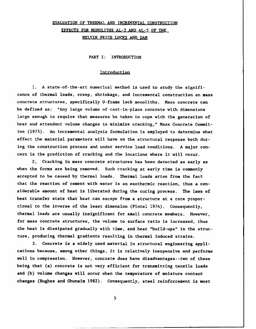
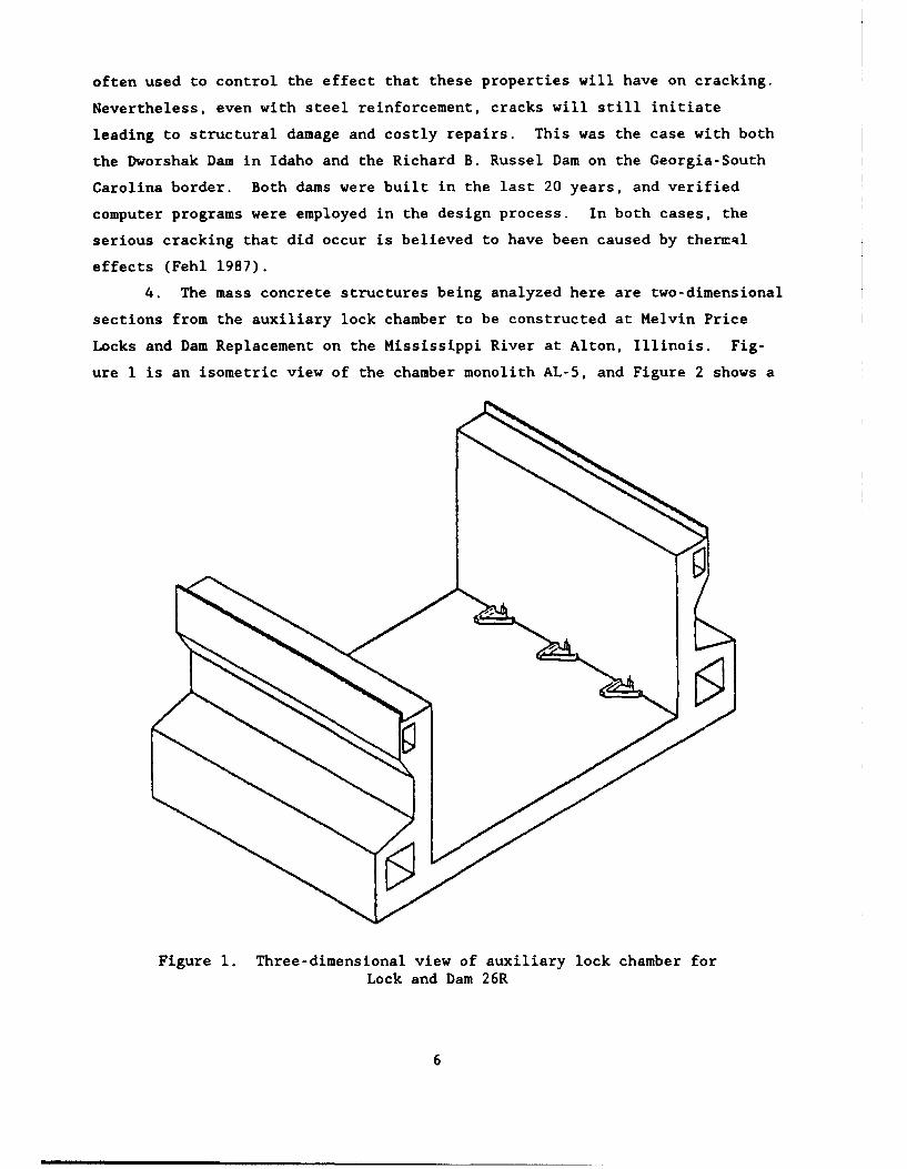
4. The mass concrete structures being analyzed here are two-dimensional
sections from the auxiliary lock chamber to be constructed at Melvin Price
Locks and Dam Replacement on the Mississippi River at Alton, Illinois. Fig-
ure I is an isometric view of the chamber monolith AL-5, and Figure 2 shows a
Figure 1. Three-dimensional view of auxiliary lock chamber forLock and Dam 26R
6
F- F- F- F- - F-IF-DIL I 0IL IL ..... . .L L L
.~ J -1 J. IiC
U)
0'4.1
$4
0
-'-4
4.40
0"-'4
i'A
9 )
" "14
ISOMETRIC
Figure 3. Three-dimensional view of lock monolith AL-3 for Lock andDam 26R
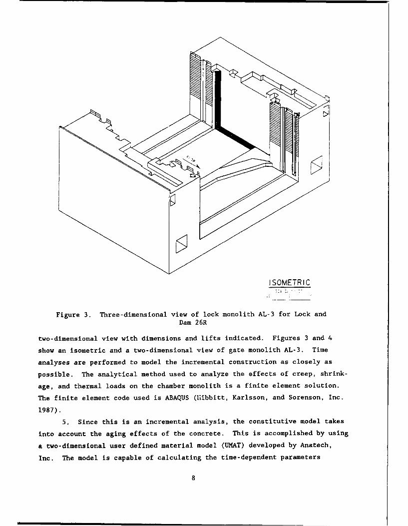
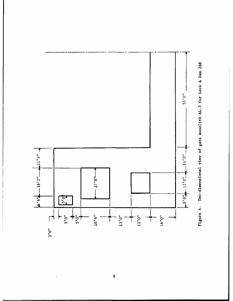
two-dimensional view with dimensions and lifts indicated. Figures 3 and 4
show an isometric and a two-dimensional view of gate monolith AL-3. Time
analyses are performed to model the incremental construction as closely as
possible. The analytical method used to analyze the effects of creep, shrink-
age, and thermal loads on the chamber monolith is a finite element solution.
The finite element code used is ABAQUS (Iiibbitt, Karlsson, and Sorenson, Inc.
1987).
5. Since this is an incremental analysis, the constitutive model takes
into account the aging effects of the concrete. This is accomplished by using
a two-dimensional user defined material model (UMAT) developed by Anatech,
Inc. The model is capable of calculating the time-dependent parameters
8
U~
0
0
-0Lr) (4-4
cn
0
0
Is
44G)
4'44
"-4
0
C'-4
1-4 r-4 -4
ot C) 0
C*I -n
enW 1___ L
important to the analysis. Thus, the effect of creep and shrinkage is
accounted for in the analysis with the creep and shrinkage functions being
based on laboratory test results. Also, the change in Young's Modulus with
time is calculated to update the stiffness matrix for each increment.
Finally, the subroutine is capable of determining when a crack occurs, and
then updates the stiffness matrix.
Oblective and Scope
6. The primary objective of this study was to gain a better understand-
ing of the effects of creep, shrinkage, thermal loads, incremental construc-
tion, and their effects on mass concrete structures. This was accomplished by
performing a parametric study using upper and lower bounds on the creep and
shrinkage functions as well as the adiabatic curve used to produce the heat of
hydration as a function of time. Several load cases were run varying the
three parameters among the upper and lower bounds in order to determine criti-
cal loading conditions. In addition, several load cases were run in which
some of the parameters were isolated by neglecting their effects in the analy-
sis process.
7. When the analyses were complete, the results of the various load
cases were analyzed to determine which of these parameters had a significant
effect on the structure. The worst realistic load case was determined so that
the analysis could be extended to service load conditions and used as the
primary load case for monolith AL-3. Also, a static analysis was performed
applying only gravity and service loads. An assessment was made on the
effects of the residual stresses from the incremental analysis process, with
creep, shrinkage, and thermal loading included, compared with gravity turn-on
coupled with service loads.
8. This report is basically divided into three sections. Parts I-III
provide basic information on modelling and material properties. Parts IV-VIII
are related to parametric studies performed on monolith AL-5 to assess the
effects of thermal loads, creep, shrinkage, incremental construction, and
their short and long term effects. Parts III and IX are related to the model-
ling and incremental construction of monolith AL-3. This monolith was tar-
geted as a place where potential savings could be found through increased lift
heights. Prior to analyzing this structures for both 11 and 16 lift
10
construction schedules, several other parameters were studied as shown in
Parts IX through XI.
9. The results obtained are a first step in developing guidelines that
can be used by the engineer when performing the design and analysis of mass
concrete structures. Also, from the work performed, improvements can be made
in the thermal stress analysis procedure. This includes modelling techniques
and the implementation of such techniques.
11
PART II: MODELLING AND MATERIAL PROPERTIES FOR MONOLITH AL-5
Introduction
10. Modelling and computer implementation to represent what physically
occurs to the structure onsite is extremely important, if accurate results are
to be obtained from an analysis. This requires both an accurate model of both
the chamber monoliths, the construction procedure, and the material
properties.
Basic Concrete Properties
11. The input data used for the thermal and mechanical properties of
concrete were obtained from previous studies for Melvin Price Locks and Dam by
the US Army Corps of Engineers (Norman, Bombich, and Jones 1987). The con-
crete is assumed to have a nominal compressive strength of 3,000 psi* using
Type II cement with a maximum heat of hydration limit (70 cal/gm) and 25 per-
cent replacement by solid volume of pozzolan (fly ash).
Modelling for Heat Transfer Analysis
12. The convection coefficient used at the exposed surfaces in this
analysis is based on a forced convection mode. This is a result of the fact
that as the fluid (air) flows over the surface with some velocity, heat is
carried away producing a temperature gradient (Holman 1981). Thus, the coef-
ficient is approximated, for exposed surfaces, by using an equation that is a
function of the mean wind speed velocity.** Radiation heat transfers due to
solar effects were neglected.
13. The convection coefficient for external surfaces is based on a mean
velocity speed of 10 mph. For the unenclosed culvert and access void, a
velocity of 1 mph was used since it was assumed that the unenclosed void would
be exposed to and ventilated by ambient air; however, the air flow would be
* A table of factors for converting non-SI to SI (metric) units of measure-ment is presented on page 4.
** Personal Communication, July 1987, Tony Bombich, US Army Engineer Water-ways Experiment Station, Vicksburg, MS.
12
rediced (Norman, Bombich, and Jones 1987). In addition, inside the voids, air
elements were used to simulate the effect of air fair actually being there.
To simulate the effect of the forms on external, vertical surfaces and for the
culvert walls and roofs, a coefficient was calculated based on the type and
thickness of the forms used. The coefficient used was based on the insulating
effect caused by 3/4-in. plywood forms. An inch of wood is equivalent in
insulation value to about 20 in. of concrete. The forms were assumed to be
removed 2 days after the lift was placed. The forms are not actually removed
at 2 days on the job site; however, this should result in a greater probabil-
ity of surface cracking since the peak temperature at the surface is obtained
near the same time as when the forms are being removed. This will cause a
sudden cooling at the surface by the environment. Thus, a steeper gradient is
produced causing higher tensile stresses.
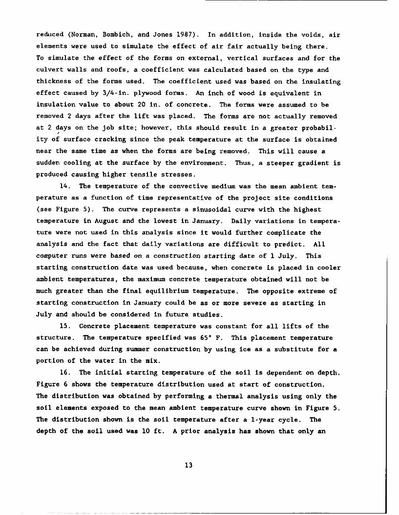
14. The temperature of the convective medium was the mean ambient tem-
perature as a function of time representative of the project site conditions
(see Figure 5). The curve represents a sinusoidal curve with the highest
temperature in August and the lowest in January. Daily variations in tempera-
ture were not used in this analysis since it would further complicate the
analysis and the fact that daily variations are difficult to predict. All
computer runs were based on a construction starting date of 1 July. This
starting construction date was used because, when concrete is placed in cooler
ambient temperatures, the maximum concrete temperature obtained will not be
much greater than the final equilibrium temperature. The opposite extreme of
starting construction in January could be as or more severe as starting in
July and should be considered in future studies.
15. Concrete placement temperature was constant for all lifts of the
structure. The temperature specified was 650 F. This placement temperature
can be achieved during summer construction by using ice as a substitute for a
portion of the water in the mix.
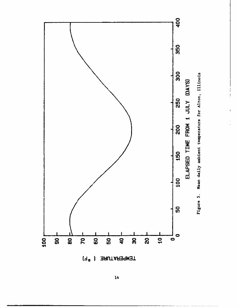
16. The initial starting temperature of the soil is dependent on depth.
Figure 6 shows the temperature distribution used at start of construction.
The distribution was obtained by performing a thermal analysis using only the
soil elements exposed to the mean ambient temperature curve shown in Figure 5.
The distribution shown is the soil temperature after a 1-year cycle. The
depth of the soil used was 10 ft. A prior analysis has shown that only an
13
0r
U)'-4
0In >- 4
54-
0
o4
LL
" "4-
C3
U)
CL4
< U4
Z4)
o o0 00 0 0 0 0 0 0
(1. 3wnif±V3dHWJ.
14
0
20
w 40
z
I-j-J
o 60CnU.
0
I-.
a."U 800
100
12050 60 70 80
TEMPERATURE ( OF)
figure 6. Soil temperature at start of construction
15
insignificant amount of heat flowed past this depth. The initial temperature
of the air was 750 F.
17. A placement rate of 5 days was assumed for each lift with the form
work being removed after 2 days, as previously stated. This rate is the maxi-
mum allowed by the specifications; whereas, actual lift placements proceed
much slower. However, this rate will produce higher stresses especially near
lift surfaces since this is the time when peak temperatures are obtained.
Consequently, a higher thermal gradient is obtained producing higher stresses.
18. Lift heights used were provided by the US Army Engineer District,
St. Louis. There are 8 lifts in the monolith. Lift heights for the base slab
are 5 ft; whereas, heights for the chamber wall vary from 4 up to 15.5 ft.
Higher lifts are obtained in the wall since the thickness of the members
decreases. The actual lift arrangement is shown in the finite element mesh in
Figure 7.
19. The heat of hydration as a function of time was obtained by deter-
mining the adiabatic temperature rise for a laboratory test specimen. The
upper bound adiabatic curve is for a mixture having heat generation due to
hydration of cement of 70 cal/gm; whereas, the lower bound is 53 cal/gm (see
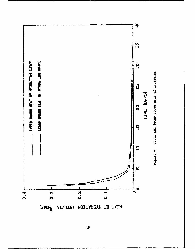
Figure 8). Note that most of the temperature rise occurs in the first 5 days.
The heat of hydration can be calculated by:
Q = CpAT/At (1)
where
C - specific heat
p - density
AT - change in temperature
At - change in time
The upper and lower bound heat of hydration curves are shown in Figure 9.
20. Looking at Figures 1 and 3, we can see that the structures are
geometrically symmetric. Obviously, the results for the thermal analyses will
be the same for the right half and the left half of each structure for the
assumptions used (i.e. neglecting solar effects, and assuming wind speed is
constant over all exposed surfaces for calculating the convection coeffi-
cient). Thus, only one-half of the monoliths needs be modelled. For a heat
transfer analysis, a boundary condition is invoked that allows no heat flow in
the horizontal direction across the line of symmetry.
16
m CD (1 I ( CUi~
F- - ILL LL LL LL ILL L L
En - - -H - - H - -H -UU
Ii.
LL I II IM
00
In
4 ~41Ca 'a
H IU
zH i HI
0
01 1 -IM
In ,4
17
0
a m
4)
c1J 4
u i 4)1-4
I'- U
0 .Q "J
0o 00
'o
0
o-
I qC4
1\n
0 0 0 0 0 0 0
18
0
IL,
> >u
00
Z 10LO >1
I-. .0-ii I44
cJuJ0
q44
I "-4
ILD r14
(CA'CI-c NI/fl.L) NOIJNVICAH AO0 IV3H
19
21. The values of the material properties and convection coefficients
used in the thermal analysis are given in Table 1. All of the above mentioned
properties and parameters are capable of being modelled by ABAQUS. The heat
of hydration for each time increment was calculated using a subroutine called
DFLUX. This subroutine was written explicitly to handle the incremental con-
struction process.
Modelling for Elastic Stress Analysis
22. The entire Melvin Price Locks and Dam structure is founded on
H-piles. The pile arrangement and stiffness for the chamber monolith were
supplied by the US Army Engineer District, St. Louis, and are shown in Fig-
ure 10 and Table 2. Pile stiffnesses for a strong soil pile support were used
since greater restraint would be provided (Headquarters, US Army Corps of
Engineers 1983). The actual finite element model is a section perpendicular
to the direction of flow and was analyzed as a plane strain problem. As we
can see from the figure, piles are arranged in rows parallel to the direction
of flow, and the number of piles in the row varies. The piles were modelled
in the analyses by using linear springs. The spring stiffness was obtained by
finding the average stiffness of each row of piles per inch thickness. The
spring stiffnesses used in the analyses are given in Table 3. Note that the
value of the spring stiffness at the symmetric boundary condition is reduced
by one-half.
23. Previous thermal studies by WES were performed with the soil ele-
ments removed during the stress analysis. At early times, this analysis
showed excessive displacements at the bottom of the structure that do not
actually exist. The large displacements are a result of the concretes low
strength after placement and thus its inability to effectively distribute the
loads between the piles. However, during construction, the site is dewatered;
thus, the soil does provide some restraint both horizontally and vertically.
Consequently, the soil elements were included in the analysis performed here.
The material properties used are representative of the soil found on the site.
The value of Young's modulus used is 3,000 psi, and Poisson's ratio is 0.35.
When service loads were applipd, the soil elements were removed since Young's
modulus would be greatly reduced due to saturation of the soil.
24. Accurately modelling the roof of the voids is extremely important
since internal galleries are a main source of cracking in mass concrete
20
I - 4..,
Li 4
ILai -C
a 44
t.0o
IFLOW
%-Snag? PI oW
21J a
(Rawhouser 1945). To leave the roof unsupported at early times after place-
ment would result in unrealistic displacements and high stresses. Applying a
fixed boundary condition would provide more restraint than actually exists and
would force the walls into an erroneous state of stress. Thus, a subroutine
was written called multiple point constraint (MPC) which allows individual
constraints to be imposed on an arbitrary degree of freedom with the displace-
ment being specified by some function with respect to two referenced degrees
of freedom. When the constraint is imposed, the associated degrees of freedom
are removed from the system matrix. In addition, the subroutine also cal-
culates an array of derivatives required in order to redistribute the loads.
The displacement function used produces a linear displacement in the vertical
direction between the nodes at the top of the walls of the culvert and gal-
lery. The constraint was removed 7 days after the lift was placed. When
constructing the monoliths, a rigid box frame is placed to form and support
the voids.
25. At the symmetric boundary condition, a restraint was applied to
prevent movement in the horizontal direction but was left free to move in the
vertical direction. The bottom of the soil was also prevented from moving in
both the horizontal and vertical direction.
26. Thermal loads primarily depend on the change in temperature, the
coefficient of thermal expansion, and Poisson's ratio when plane strain condi-
tions are assumed. The value for the coefficient of thermal expansion used in
the analysis was 4.5x10. 6 in./in. * F (Fintel 1974 and US Army Corps of Engi-
neer District, St. Louis 1988). The value of Poisson's ratio used was 0.17.
This value was assumed to be constant.
27. Gravity loads (body forces) were turned on 1 day after the lift was
placed. Prior to 1 day, a distributed load was placed on the lift below to
simulate the effect of the new lift. The loads were applied in this manner
because of the low strength of concrete before 1 day and because time of set
does not occur until about 12 hr. If the loads were applied when the lift was
placed, the concrete would flow out the vertical face. During the actual
construction process, the forms would provide the restraint to prevent this
since a body force truly exists.
28. The service loads applied are shown in Figures 11 and 12. Service
loads were applied 102 days after start of construction or 67 days after the
last lift was placed. This amount of time was chosen since the thermal loads
22
.jn
CY)
In-
00
Uu
-j4
CL/i
I-
I-.LIII
(4 4
Q Q0
>-
tz U
23
0 w
CC,
-4
UU
00 ".4-LL..
z '
-w 0
'--4
0i
z
'--4
$.4
4-4
GI N- V)i
LI "
244
had dissipated and any residual effects were considered to have stabilized.
The loads represent backfill in place, upper pool at el 419 ft above sea
level, upper pool elevation in lock, tailwater at el 395, minimum uplift pres-
sure, 0.l-g earthquake force directed toward the Missouri side, and an equiva-
lent concentrated force due to the effect of the water and backfill during an
earthquake. The concentrated forces shown in the figures were actually
applied as a uniform pressure over two of the element faces to avoid a stress
concentration.
Mesh and Element Selection and Time Frame
29. As stated previously, the size of the elements and time step will
determine how fast the solution process will proceed and the amount of error
in the solution. For the finite element method, the error in the solution
decreases as the size of the largest element goes to zero. Thus, proper mesh
refinement and using a suitable time step is important to assure the quality
of the results and also to minimize computing time and space.
30. In addition to choosing the element size, the element type also had
to be selected. ABAQUS element library includes both eight noded and four
noded quadrilateral elements for both heat transfer and plane strain stress
analysis. Eight noded elements are generally preferred for linear analyses
because larger elements can be used, thus reducing the number of elements in
the mesh, while still producing good results. Four noded elements are pre-
ferred for nonlinear analyses if the size of the element is sufficiently small
enough to capture the nonlinearity. The same mesh and element type was used
for both the thermal and stress analyses, because the stress analysis uses the
temperatures calculated in thermal analysis to determine the thermal induced
stresses. The eight noded element was preferred in this study since fewer
elements could be used to generate the mesh and because studies previously and
currently being performed by the US Army Corps of Engineers also used the
eight noded elements; thus, comparing results would be simpler. The eight
noded element can also be used with either nine or four Gaussian quadrature
points for the stress analysis. Earlier studies by WES showed that nearly the
same results were obtained when the reduced integration option was used.
Therefore, the reduced integration was used in the analysis performed here so
as to reduce computing time and space.
25
31. ABAQUS also offers interface elements for both heat transfer and
stress analysis. The one-dimensional heat transfer interface element allows
the user to prescribe the conductance between different materials placed
against each other. These elements can be useful at the soil-concrete inter-
face and lift interfaces. The elements were, however, only used between the
soil-concrete interface. The reason for this was due to the fact that the
common node shared by the top of the soil element and the bottom of the
concrete element can only be prescribed one initial temperature. However,
with the interface element, the soil and concrete nodes, at the interface, can
be given their respective starting temperature. The interface elements were
not used between the lift interfaces.
32. The time step established by Waterways Experiment Station (WES) was
also used in this analysis. The time increment used was one-fourth day for
the first 2 days and one-half day for the next 3 days after a lift was placed.
A 5-day time step was used to run the analysis to service loads. This time
step works well to achieve the basic tolerance measure for the solution of the
equilibrium equations at each increment without requiring an excessive number
of iterations (Hibbitt, Karlsson, and Sorenson, Inc. 1987). The program
allows the user to specify the tolerance level, the number of iterations
allowed in an increment, and the ability to have the solution continue even
though the tolerance level was not achieved in the allowed number of itera-
tions. The tolerance level used was 10 lb with 20 iterations allowed in an
increment. After lift 4 was placed, only the first increment did not con-
verge. Note, however, that this occurred when the MPC was first applied, and
that the program calculated the residual force to be approximately 15 lb. It
was estimated that 10 more iterations would be required to achieve conver-
gence.
33. The numerical stability of the heat transfer analysis can be
assured by following a simple prederived stability criterion. With the time
step being established, the element size can be determined by equation:
At > (pCl6k)AL 2 (2)
where
p - density in lb/ft 3
26
C - specific heat in Btu/lb °F
k - thermal conductivity in Btu/(h - ft °F)
AL - element dimension in the direction considered in feet
At - time step in h (hr)
The maximum element size for concrete material is 27.76 in. and for soil mate-
rial is 16.70 in. when the eight noded element is used. Preliminary analyses
were performed with the element size violating this equation which provided
unusual oscillations in the results from the heat transfer analysis. Conse-
quently, several analyses were made using an 8 ft thick by 80 ft long flat
slab founded on 10 ft of soil with the various elements and sizes shown in
Figure 13. For mesh IV, the interface element was also used between the soil
and the concrete. The same material properties and parameters were used as
outlined above but a different adiabatic curve was used which produced higher
temperatures, and the initial soil temperature was constant throughout the
depth at a value of 550 F. The results are shown in Figure 14.
34. The results shown are at the center line of the slab, 6 hr after
the lift is placed. The results show that the element size should not violate
Equation 2 in the direction of heat flow to prevent unrealistic oscillations.
However; toward the middle of the slab, the element size can be increased in
the horizontal direction since heat is flowing only in the vertical direction.
It was found that an aspect ratio of two is acceptable in this area. The
finite element mesh used for the chamber monolith was shown in Figure 7. The
mesh has 328 soil elements, 37 interface elements and 51 air elements (used in
heat transfer analysis only), and 445 concrete elements.
27
CONCRETE ELEMENT SOIL ELEMENT
24 99MESHI ±
1- ----2I~40,B MESH II s0U_ ._Le V1 -
DMESH IiiII 30
,I
D MESH V
L-e-
4 MESH V j .
Figure 13. Element dimensions used to select mesh
layout, in.
28

96-
72- MLES H ITII
MESH LIV & V48-7/- II S
U 2 " - : _ n _T
I', MMI ---Ui5
C1 -15-
0 -30
-45
--60--
-105 -
-12050 60 70 80 90 100 110
TEMPERATURE, OFFigure 14. Temperature distribution for 8-ft slab using
various meshes
29
PART III: TWO-DIMENSIONAL USER MATERIAL MODEL FOR TIME DEPENDENT
EFFECTS OF CONCRETE FOR MONOLITHS AL-3 and AL-5
Introduction
35. The important time dependent effects include creep, shrinkage.
Young's modulus, and cracking. One of the reasons for performing these analy-
ses is to predict the significance of creep and shrinkage on mass concrete
structures. Thus, how the creep and shrinkage functions are modelled is a
major concern. The equations presented here were generated by WES (see
Norman, Bombich, and Jones (1987) for a more detailed description). The two-
dimensional user material subroutine UMAT was developed by Anatech, Inc.,
under the direction of WES. The values for the upper and lower bound of creep
and shrinkage were decided upon at the Thermal Stresses in Mass Concrete
Structure meeting in July 1987 to account for variability in test results.
Shrinkage
36. The type of shrinkage used in the model is autogenous shrinkage.
Autogenous shrinkage is internal drying due to heat of hydration and may
account for up to 95 percent of shrinkage effects in mass concrete. Drying
shrinkage, however, was neglected in this analysis.
37. Autogenous shrinkage is largely a result of the chemical process
that occurs during curing of concrete. This process occurs over a long period
of time, up to several years. Much of the effect of autogenous shrinkage
occurs in a short time after the lift is placed. The shrinkage process is
also a volumetric process since curing is assumed to take place at the same
rate throughout the lift, then shrinkage results equally in all directions.
38. The shrinkage strain equation in UMAT is given by:
e=(t) - C1(lC elt) + C2 (]_e,2t) (3)
where
C1 - 102.5 x 10⁻⁶
C2 - 72.5 x 10⁻⁶
30
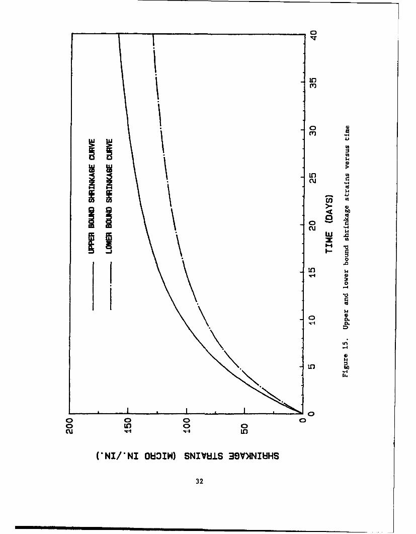
s, - -0.15
S2 - -0.02263
Figure 15 shows shrinkage strains plotted against time for the upper and lower
bound values that were used in the analysis.
CreeR
39. Creep of concrete is the dimensional change or increase in strain
with time due to a sustained stress (Fintel 1974). In freshly placed con-
crete, volume changes due to creep are largely unrecoverable; whereas, creep
that occurs in old or dry concrete is largely recoverable and appears to be
independent of temperature and stress. Creep is generally a linear function
up to a stress-strength ratio of 50 percent of the ultimate strength of the
concrete. Beyond that point, creep becomes nonlinear (Fintel 1974). In addi-
tion, the rate of creep is high during the initial period of loading.
40. Creep is related to the age of the concrete and the elastic modulus
at the time of loading, size and shape of the member, duration of the load,
modulus and volumetric percent of aggregate, temperature, and the amount of
steel reinforcement. The effect of the aggregate and reinforcement is to
reduce the overall creep effect by restraining volume changes.
41. The creep relation in UMAT as a function of time, loading age, and
temperature is given by:
2
J(t:,r,T) = - Ai(r,T)(l-e".iCt-) +D(r,T)(t-,r) (4)
where
"A(,T) I•. r=
D(,,T) - D_/'T E3)
E(r) - Eo + El(l-e-nl' lr) + E2(1-e~n2(T-1)
31
a
ILO
go CD
En I
1 I3
00LO
0
U-)
'-4)
0 0O 0 0
0*I/N U)IW 0NVI 09)NM
32
where
E(r) - Young's modulus as a function of time
T - temperature
R - gas content
Remaining values are material constants obtained from tests (Norman, Bombich
and Jones 1987). The term involving the square of Young's modulus in the
Coefficient A and D is the creep aging factor. The upper and lower bound
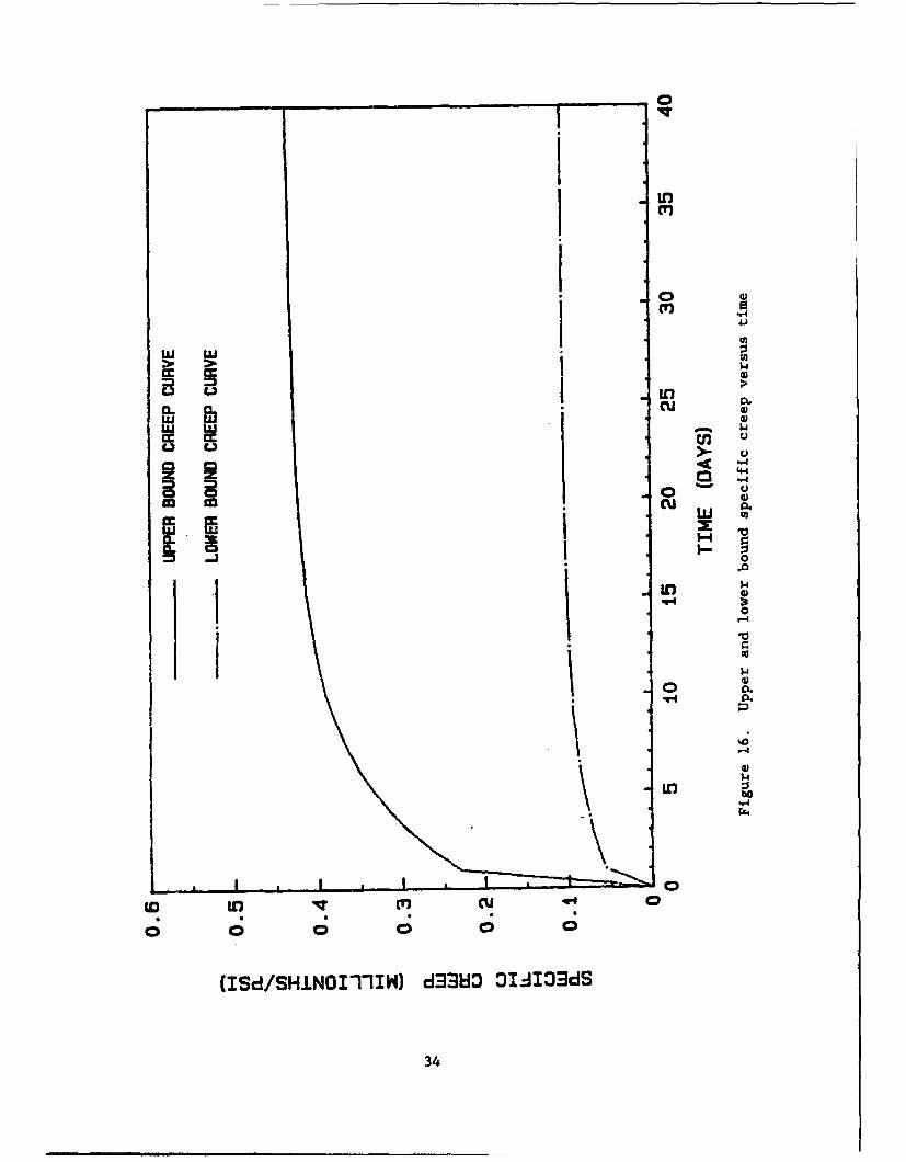
specific creep curve used is shown in Figure 16. The first term in Equa-
tion 3-2 controls the short term creep for the first day. The second term
governs the intermediate creep, up to 30 days, and the last term gives the
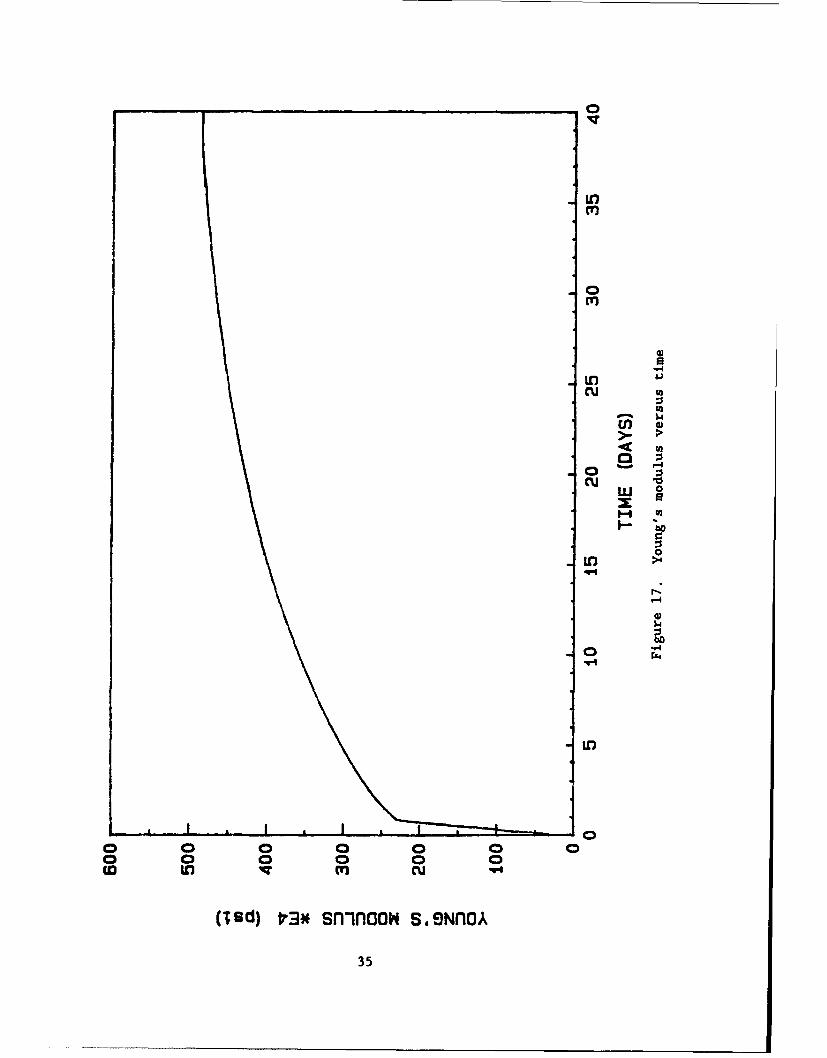
creep behavior after 30 days (Anatech, Inc. 1987). The plot of Young's
modulus versus time is shown in Figure 17.
42. With the specific creep and shrinkage function specified, the uni-
axial strain can be calculated by:t
e(t) M [i/E(r) +J(t,r,T)]o(r)IaT +aAT + e8 (5)
Thus, the stresses can also be calculated and the stress analysis is near
complete. With both stresses and strains calculated, the cracking criteria
can now be implemented.
Cracking Criteria
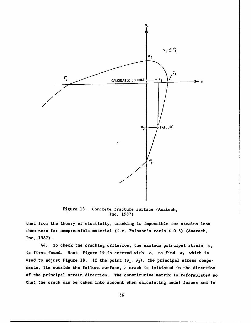
43. The cracking criterion that must be satisfied for a crack to be
initiated into the model is as follows. The criterion is strain driven but is
modified by the stress. For isotropic material, the principal strain and
principal stress direction coincide (Anatech, Inc. 1987). The two-dimensional
failure surface is shown in Figure 18. The tensile strength is calculated
using an interactive criterion since a stress or a strain criterion alone is
not general enough for a time dependent, nonlinear analysis including creep
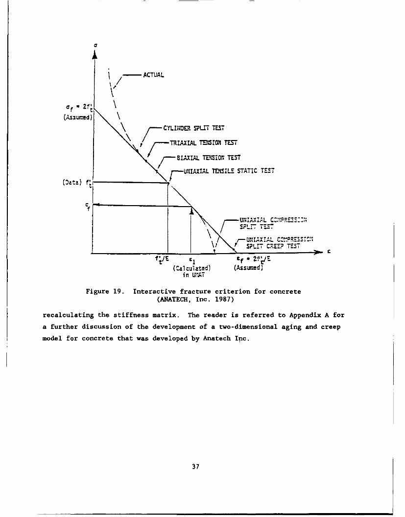
and shrinkage effects (Anatech, Inc. 1987). Thus, Figure 19 is used to relate
cracking stresses and strains based on experimental data. For simplicity, a
linear relationship is assumed. The factor of 2 is arbitrary but is used to
expand the curve above and below the midpoint (uniaxial tension test) so as to
accommodate cracking at high stresses and low strains and vice versa. Note
33
'IInCL C*1LU L
Cuu
4)
0 ra
0 0
0
Cd
00
"Z4
34
0
Cr))
9"4
cLI C
C3
%.Iv r4
0
0 -4
t II
0 0 0 Cow If) q m c
(Tsd ir3 sn-ncowS. Ono0
35L
0 ff- t
CALCULATED INl UAT-
-- 7/
a2 FAILURE
/C
Figure 18. Concrete fracture surface (Anatech,
Inc. 1987)
that from the theory of elasticity, cracking is impossible for strains less
than zero for compressible material (i.e. Poisson's ratio < 0.5) (Anatech,
Inc. 1987).
44. To check the cracking criterion, the maximum principal strain el
is first found. Next, Figure 19 is entered with e1 to find oa which is
used to adjust Figure 18. If the point (a,, 0 2 ), the principal stress compo-
nents, lie outside the failure surface, a crack is initiated in the direction
of the principal strain direction. The constitutive matrix is reformulated so
that the crack can be taken into account when calculating nodal forces and in
36
-ACTUAL
(Assured)
/-CYL1NMR SLI s- TEST
-TRIAXIAL TOSISZG TEST
BIAXIAL TENISION~ TEST
(~a~3) -UNIA"XIAL TEMISIL E STATIC TEST
U AXIA.L C:;!== _15\ /Thr ..,,,vA ,--o-•,
SSPLIT CR.EEP M-S
(Calculated) (Assz.d]in UWAT
Figure 19. Interactive fracture criterion for concrete(ANATECH, Inc. 1987)
recalculating the stiffness matrix. The reader is referred to Appendix A for
a further discussion of the development of a two-dimensional aging and creep
model for concrete that was developed by Anatech Inc.
37
PART IV: RESULTS FROM HEAT TRANSFER ANALYSIS FOR MONOLITH AL-5
Introduction
45. The temperatures at selected nodes in the finite element mesh will
be presented and discussed. The nodal temperatures are plotted against time.
The time scale is relative to when the node is activated in the analysis pro-
cess, or time zero corresponds to when the lift is placed. The solid lines
are the results from the analysis using the upper bound adiabatic temperature
rise curve (70 cal/gm), and the solid-dashed lines are the results when the
lower bound adiabatic temperature rise curve (53 cal/gm) is used to determine
the heat of hydration. The small circle on the monolith indicates the approx-
imate location of the node and the top of a lift is indicated by the horizon-
tal lines. Figure 20 shows the finite element mesh again with some of the
nodes and elements numbered for reference of exact locations of the nodes.
Figures 21-34 are temperature versus time plots at locations near the Gauss
points where stresses were investigated. Figures 35-37 are presented because
of their significance to the heat transfer analysis.
Discussion of the Heat Transfer Analysis Results
46. Figures 21-34 are broken into three groups. Figures 20-25 are at
nodes that are at the top of a lift when placed but become imbedded in the
model when the next lift is placed. Figure 25 is a node at the soil-concrete
interface. The nodes in Figures 26-34 are on the surface and always remain
exposed to ambient conditions.
47. From Figures 21-24, the following patterns can be identified.
After the lift is placed, a large temperature rise occurs in the first day due
primarily to convention since the temperature of the surroundings during
placement of all lifts is approximately 80° F. The temperature then remains
constant at a temperature just slightly above 80° F until, at 5 days, another
temperature rise occurs due to the placement of the next lift. This tempera-
ture rise is primarily a conduction process due t; the heat liberated from the
newly placed lift. The peak temperature is obtained at approximately
9-10 days after the lift is placed. The peak temperature is around 95° F.
After the peak temperature is obtained, the temperature decreases in an
38
(r)4 wq 4 wo 1 a CD tocuW cu i) CU 'r m m
I)I cu 0 r. N C') (IPit' m m (TI cu cu ri Wt4
z z z z z z z z z
I I I IW I b
ICIS1.1I
11.0
[i II I I I
a) N- 1N N to in CII T4
ULJ w ~ i hLI bJI hJI hJI I
39
0In
oz zo to inI
wU w ea. 0oL 0 0
-J / 0
I 0n
cw
I.L
a UJ
1 04
0~~~~I InIm c c r% rl
Io uiHd3
400

0
z z
m m 1
w wL
a.a
> 0
ccu/ 0 ~ " 4 .-1i (w,2o
0 ý0
In r-I
cu I4
M 44
o 1 if)
z 1- 4
/ If)
$4
E-4
1 ')
0) 01
z zo 0 in
CJ
- 0%
0.. 0 0M s-I
'4-'
U) C
>- .0CU
a 0dJw
01 1 >- -
z I 0
"4)
in
C4.
(.4 minv~l~d.4
42.
z zo 0 i
cv"
w wU IoL 0
0
14-
Cr))
II
1 WN I 0
Cr) /w * W
11
CU1
43.
In
z z0o o W)-
CL 0r
D -1 5 41014
In
5.)
cn0
wI 0I In ' ý4
I I-
cu < 1
w0"4.
LI)
1.4
44.
0
z z
CV)
w w C14
0
14
L~v~i~jJ%
wu w0 I- 0
cu to ýJww
W 6)
>n
0
'-a
a)
C.,4
0 in 0 M) 0r 0L 0 4
0 ) En 0 w N w wD 96
45
z zo 0 i
-co*
cr LI-w w 4
a. 0
0I ~44
I 4C)
I En
".0'U
oD 'u
CDc'U
w w e> > 4
0 m 4-
1 01
0m
ILD
46
z zo M I
0 00
CL 0 0
34-
0
I 1-4
(D 0)
OD x- 0cu If)cu
L U I> 1-4
z I0
W o)4.,
'4' )
47-
z zo 0 1g*) CN.
w w 4)
a. 0 r0:3 -11
0
1w 44
Cuw 4)0
N-4cu r
o C)
1cu _jW0
I C))
24)
4),
raw
48
o 0
z z
MI M
w w CCL 3 0
M~ 0 0
0I (4.4
04"4
Cud
o'
0< 0
w wI e~d> 4.4
w0
.q-4
$42
W4 44
U 3wn.Lb13d.'
490
0
z z
tn w
CL 0
:3 -j
44'
>- C)-4
0< 0
cIn'- (4o
C)d
cu -4
C c )09
.v.14
50)
z zIn v-4
o 0
0. 00~$0
U) U
z 0
Wl LIJ co > '-4
z0
W 0m 4
4.)
"4$4)
4)
04IdI$
"tn0 01 In 0 n -09
51
z z
w w 0)
a. o 0
0t41
0< 0r-
-j 5
tu
Cu j
'-4
522
z z
(N
w w C0.. 0
0.. 0
0
I 4-i
cuu
0*
cu2
Cu z 4'
CIId
44
In
4.30 M D co cc N Pý- D Uk
"q)
3kinJLW~d14
53'
0
z z
C.,4
cr. ccLw w CN,
0
InC") u
in 0
w w> 54
04 0
U)
/ 03'.4
in)
/ 010 o wt
q-54
0
z z
- I f ),
c c C14w w I 0
M 0V
3 5 0
UUrn uI '-I
/ 00
zz
C 4-4
CUrI W l
I CD cn co w N r* D UW4 rW o
u~~c aini-'d3
550
in
z z
m M)a. 00
=in LJ*n
CI 0r
/ 0 0
in 0d
IL
z/0/ ~cu _jI'.
wi 0
cc 44I
tnn
Cu
1-4
ca,
a) 0y) w r- P. to CD--4.44
56
exponential fashion until thermal equilibrium is obtained. Obviously, the
analysis using the upper bound heat of hydration produces higher temperatures
in the structure. Also note that, for the lower bound temperature graphs,
just after the next lift is placed (after 5 days) a small decrease in tempera-
ture occurs. This is a result of placing cooler concrete (recall that con-
crete placement temperature is 650 F) on top of the older concrete and also
since enough heat is not liberated initially to produce an increase as in the
upper bound temperatures.
48. The temperature increase shown in Figure 25 is predominantly a
conduction process. Since this is at the soil-concrete interface, part of the
initial increase in temperature of the concrete is due to placing the cooler
concrete on the warmer top soil (Figure 21). The remaining temperature
increase is due to the heat liberated by the concrete. Note that after the
peak temperature is reached, the temperature remains fairly stable since the
soil acts as an insulator but not a good insulator--otherwise, the peak tem-
perature would be about 10° higher.
49. Figures 26-34 show a predominate convection process since the nodes
lie on the exposed surfaces. In Figure 26, a decrease in temperature occurs
after 5 days. This is a result of activating air elements when lift 3 is
placed. The initial temperature of the air elements is 750 F, and it can be
seen that the concrete elements take on the same value. Note also that the
same node is shared by the concrete and air elements. The use of air elements
and convection coefficients inside the culverts proved to be an inaccurate way
to model what happens in this area. It can be seen that after the air ele-
ments are activated, they draw heat out of the system at a rate that is not
realistic. If air elements are to be used, the material properties need to be
reconsidered. The use of gap elements between the air and the concrete may
also be required instead of using convection coefficients. However, this
would only complicate the analysis while the use of convection coefficients
alone at these surfaces should model what occurs there well enough. The
decrease in temperature at 7 days is due to removal of the form work placed
around the entire culvert. The decrease at 10 days is related to completely
closing of the void. With lift 4 being added to the system, (with a 65° F
placement temperature) the temperature of the air elements inside the void
decrease thus causing the surface of the concrete to decrease slightly in
temperature also.
57
50. In Figure 27, the node quickly takes on the temperature of the air
and remains the same as the ambient air temperature. In Figures 28-32, the
decrease in temperature at 2 days is again due to removing the form work, thus
more heat can flow across the surface. The decrease in temperature in Fig-
ures 29 and 32 at 5 days is again related to using the air elements.
51. Looking at Figure 33, only a slight drop in temperature occurs when
the form work is removed. This is again a result of the air elements. Since
the void is much smaller than the culvert, there is less air to be heated, and
it takes on a higher temperature. When the forms are removed (after the void
is completely closed), heat flows back from the air into the concrete produc-
ing a smaller decrease in temperature. Again, this indicates that the use of
the air elements may be need to be reconsidered in future studies.
52. Figures 35, 36, and 37 are presented because they show the tempera-
ture variation for nodes imbedded within a lift and they show the difference
in the peak temperature will depend on the member size. From Figures 35 and
36 we can see that both nodes are in the center of the member and that both
lifts are 12 ft high (Figure 28). However, node 2525 is in the center of a
5 ft thick member; whereas, node 2544 is in the center of a 8 ft thick sec-
tion. Thus, node 2544 obtains a temperature approximately 4° F higher than
node 2525 since the thicker member generates more heat and dissipates it
slower. In Figure 37, the temperature for the node that obtained the highest
temperature is shown. This temperature was reached 5 days after the lift was
placed and the temperature was 98.5° F. This maximum temperature compares
well with analyses performed by other people in this area of work (for exam-
ple, see Fehl 1987). It should also be noted, that it took approximately
80 to 90 days to dissipate most of the heat generated within the monolith
during the construction process.
58
PART V: STRESS ANALYSIS RESULTS VARYING THERMAL LOADINGS
Introduction
53. The nodal temperatures, generated from the thermal analysis, are
stored in a file so that during the stress analysis, the program ABAQUS, can
access this data to calculate the thermal induced strains. In addition, the
time dependent material properties are made available for the stress analysis
by calling a FORTRAN subroutine, UMAT, prior to assembling the stiffness
matrix which is then used to determine the thermal, creep, and shrinkage
strains. Thus, two separate nodal temperature files were created during the
heat transfer analysis by using the upper and lower bound adiabatic curves
shown in Figure 8. Therefore, two stress analyses were made with creep and
shrinkage fixed at their respective lower bounds while the two temperature
files were used so as to select the adiabatic curve which produces higher
tensile stresses. This adiabatic curve was then used in the remaining stress
analyses where the degree of creep and shrinkage was varied.
54. In this section, the results that were used to select the adiabatic
curve and also the results of analysis made where thermal loads were neglected
to show the significance of performing a time dependent thermal analysis simu-
lating the construction process of a mass concrete structure will be
presented. In the following part, the results of the various analyses with
the different load cases (i.e. creep and shrinkage) will be discussed.
Table 4 shows the various load cases that will be examined. It should be
clearly noted that the location of the stresses presented are at the integra-
tion (Gauss) points and not at the nodes as were the temperatures shown in
Part IV. Thus, the actual temperatures used to compute the thermal strains
are not exactly the same since the integration point is located at a distance
X from the edge of the element where X is given by:
X = L/2 - (L/2)/(r2) (6)
where L is the dimension of the element. Note also that the sign convention
used is that positive is tensile and negative is compression.
59
Discussion of Stress Analysis Results Varyingthe Degree of Thermal Loading
55. Figures 38-51 show the results for loads cases 1, 2, and 3. In all
the figures, we can see that for load cases 2 and 3, just after the lift is
placed, the stress is compressive. This is due to the heat increase, thus the
element wants to expand but internal restraints prevent it from freely expand-
ing, and compressive stresses result. However, quickly the stress becomes
tensile due to subsequent cooling of the concrete. In all the figures except
Figure 41, neglecting thermal loads produces significantly lower stresses and
most of the figures show for load case I that the stresses are predominantly
compressive.
56. Figure 38 shows a situation where the stresses are mostly due to
bending. Looking at Figure 10, we can see that the location is between two
piles. The bottom of the slab acts like a continuous beam, transferring the
loads into the piles. The soil does provide some support; however, it carries
a small amount of the load (from the analysis, it was found that the soil
carried about 25 percent of the load). The increase in stress at every 5 days
is a result of placing new lifts.
57. The increase in the stress in Figure 39 for load case 2 and 3 at
5 days is a result of the drop in temperature due to activating the air ele-
ments (see Figure 24). The stress then decreases due to the increase in tem-
perature, and then the stress increases again due to cooling. Looking at
Figure 40, the stress decreases at every 5 days due primarily to a bending
effect and also partially due to a Poisson effect of adding the weight of the
new lift. For load case 2 and 3, an increase in the stress occurs after
5 days due to the additional heat being added to the element from the new
lift.
58. Figure 41 shows the stress at the symmetric boundary condition. At
this location in the structure, the thermal loads aid in reducing the stress.
This is a result of the thermal loads causing the element to expand but the
center-line support prevents the element from expanding to the right, provid-
ing a greater compressive stress initially which reduces the tensile stresses
that result later. Looking at Figure 27, we note that the tensile stresses
resulting are not related to the thermal effects since no significant drop in
temperature occurs. The stress increases every time a new lift is placed
60
4 .4<
000
Iu 0
cu bo
> >
1- w
1-4
L--AU
1-1
U)U) a)
if)
000 L
0
1u -i 0I2 ,v I
> >1
-4
DI4
z cu V
HId MUI 0 X 0Z~dO
62. .
000 -
000 I 1
I 0
I4 1
1r >- ICU 04
ii boID cu W ,
_j 0
'41
LO
rz 0
cn cu c(I~d)SS381 -IVIOZI-4
63J
____ ___ ___ ___ ___ ___ ___ ___ 0
u)cn u)ci
O D D 1.3 C.li<44c 4t 00
000 In-j -1 -1 4
0
I 10
cu < 0*m r ,
r-4
z w~
a) w .In II1 I>
1-*) 0II
'.4 LU Uii "-4
II ý4.w4Wn
0'
(ISd) SI VIOUH
in in i
000
*1 40
*~ 1:II j bo
II~ I.U, '-
I- -4I-II!
> >,
CD I
Co % ILo
II
wId S31 Il.NOI0
65)
Ii 4"'Lu) n u
000
0
in 0"
a-j Cj,
0
ý4-N I) Ca
(0 II W
Ii cuw 1* 0
'1 0r
w 4)
w0
o 0 000
(ISd) SS3815 IVINOZhI80H4
66
cncncn U).4I
000o
r-.4J r
C3 0
z / LIw LU
0 w I
Cd
w 4)
'.4
Cu '1
(ISd) SSMI1S 1lVJNOZhIOI-I
67
~000 I
cc 0 0r
0
II in
a. II,>- *
c'<CU 0I..- IIzr
cu boI! r
w iw"-4
$4
(.o
4U,
-A-- g 0
(ISd) SS381S 1IVINOZIUOH
68
-4 cu mt
"0 LMcu0
CI 0
~' !' jr-4
I. ~cu< u
z >.
w w 0
cc -4 2
w0 LLJ 4/94
>,
In 4
~ Do
f LA I I AL a I "-
(ISd) SS9281S IV.LNOZI8OH
69
____ ___ ___ ___ ___ ___ ___ ___ 0
ca.u (r)
000 HC
00
cu It 0 0
bo
C. C,),CU < 0
F- CUz I.wH
I. r.
w w4
LILLI 0
J1 41,
0 ý0
4.,
w4
(ISd) SS3WIS 1YVINOZhIO0H
70
u n cncC.) L~) L)
000 00
~ II a)
I. 0cu <Ir
iic 0 -4
-4
'-4U0 0)
_ j .J-4aU
0 0)
(ISd) SSRUIS IVJ.NOZIEIOH
71

0
'C~jP II
a -
000 1
Ii i0
In>..>- co-zu I0
I-I WQ
41I
ou I'.9 iw
0I Icuf(I~d)SS38S -IVII83
72
.... ....
____ ___ ___ ___ ___ ___ ___ ___ 0
000 81
43
0
44
i>-*l 0w
F- >.
z- 0 4in - J
II $4
1- in4 4.
zId S31 V:II ini ,
W I, q.473
___ ___ ___ ___ __ ___ ___ ___ __ 0
.wq cu (In
w w w
000 00
iiincu x 0
Ig w
co Cu
'4 IIw -Scc
w "4
w~w wl'4
ii c
(Id S8S-VIId3
74-J-
which is due to bending. Figure 42 shows similar results as those in
Figure 39.
59. Figure 43 is at a location where the multiple point constraint is
applied. For all three load cases, the resulting stress is tensile as would
be expected since the roof of the culvert is acting as a large beam. It
should be noted that no gravity loads are placed on the roof of the culvert
until after 1 day when a gravity load is applied to the elements forming the
roof. Going back to Figure 40, this is the reason an increase in stress
occurs at 11 days. No rational explanation can be given for why load case 2
produces higher stresses than load case 3 after 25 days. However, it may be
related to the fact that the Gauss point is near the corner of the culvert,
thus producing a point of singularity in the mesh where unusual results may be
expected. It may also be related to the numerical method, especially since
this is the location where the convergence criteria were not strictly
satisfied.
60. Figure 44 shows again a situation that would be compressive but,
due to thermal loading, a tensile stress result. Again, compressive stress
would be expected at this location for load case 1 since the roof of the cul-
vert is acting like a beam and this would be the top of the beam--thus, there
is a downward curvature forcing the element into a compressive mode. The
compressive stress is small due to the large size of the member and also since
it is supporting only its own weight.
61. Figures 45 and 46 are again similar to Figures 40 and 42 since the
locations are near the top of a lift and more lifts are placed above it.
Figures 47 is also a location where a multiple point constraint is applied to
support the roof until adequate strength is obtained for the concrete to sup-
port itself. The magnitude of the stresses is not as high as in Figure 43,
but the span of the roof is only 5 ft at this gallery as opposed to 12 ft for
the culvert. Also the lift height is not as thick at this location, there-
fore, less heat "build up" results. For load case 1, the stress is compres-
sive because the elements that form the roof are acting like a fixed-fixed
beam. The stress is extremely low but again the weight to span ratio is low.
62. Figure 48 shows the stress at the top of the structure. At this
location, the loading is predominantly thermal at early time since gravity
loads are nearly nonexistent.
75
63. Finally, Figures 49-51 shows vertical stresses near the culvert
vertical wall, the chamber wall, and the gallery vertical wall. Obviously,
without thermal loads, the stress is compressive; with thermal loads, a situa-
tion similar to that of an unrestrained slab is found. For load case 3, the
stress reaches a value near 150 psi which is significant since this stress is
reached at 5 days when the strength of the concrete is low, and because the
gravity loads work directly against the thermal loads in the vertical direc-
tion. The slight increase in stress at 10 days could be related to the fact
that the chamber wall up to lift 5 is bending "in" toward the chamber, produc-
ing eccentricity which induces "extra" tension after placement of lift 5. The
decreases in stress at 20 days is due to the eccentric load caused by lifts
6 through 8, thus causing the chamber wall to bend now away from the chamber.
64. Based on the above results, the upper bound adiabatic curve will be
used in the remaining stress analyses, as was expected.
76
PART VI: STRESS ANALYSIS RESULTS SHOWING EFFECT OF CREEP AND SHRINKAGE
Introduction
65. After the upper bound adiabatic curve was selected, a parametric
study of the effect of creep and shrinkage on a mass concrete structure was
performed. The results of such a study will now be presented. The various
load cases examined are shown in Table 6.1. First, the effect of shrinkage
will be assessed by looking at three analyses in which creep was fixed at the
lower bound. Shrinkage was given in Figure 15. In the third analysis,
shrinkage was neglected. Next, the effect of creep was determined in a simi-
lar manner. Then, a series of plots are presented with all the realistic load
cases (i.e. load cases 3 through 6 in which both creep and shrinkage are
included in the analysis) to determine the load case which consistently pro-
duced higher stresses for performing a service load analysis. In addition,
the strains for these load cases will also be presented since cracking in
concrete is related to both stresses and strains. Finally, locations on the
mesh where the horizontal and vertical stresses exceed a specified value at a
certain time in the analysis will be presented. There are two reasons for
doing this--first, to show areas where cracking may be critical and secondly,
to verify that the locations where stress and strain plots were examined are
the critical locations in the monolith.
Effect of Shrinkage on Resulting Stresses
66. Figures 52-65 show stress versus time with creep fixed and shrink-
age strains varying, as seen in Table 5, load cases 3, 5, and 7. Conse-
quently, the load cases with shrinkage included tend to produce lower stresses
later in time. This is the case in all the figures with the exception of
Figures 51, 55, 57, and 61. In these figures, as previously noted, the
stresses induced are predominantly due to bending effects and all four loca-
tions are near an externally applied support. Figure 55 shows that neglecting
shrinkage greatly reduces the stress. This is because shrinkage is a volumet-
ric process occurring in equal amounts in all directions. Therefore, as the
element shrinks, the boundary conditions cause the resulting force to be
77
(r) in a .n
I: U C) ,
0 00 4)4)fj 4)
4)I!ocu 4
0
H tko
'-4
W 'U
w IU
o>
41
V)
U)
Inn
4)
bo"-4-
(ISd) SS3WIS IVINOZIEIOH
78
0
Inncj ifsP
1/ LfI
000 in En
0000
bo
II co
cu .4 )
z W'I 0
ww54-
0 Co
".4
to>o
0 c0 0 0 0 0
0 0 0 0
Cr) C>
(I~d SS3.S 1INO~lIW
79n
000 I~ I I
0000
U)
II 0I- 4I
w ,
z 0LUr rlv W
LLA
LU 11
1-4
1IL
800
I0
w ww I000 IIu-
gi Ui
44
z Ii wI--.th
('u 4)
IL) ii> Up
a:-4
w
1181
0 L0
000.4 -4 .I IJ-
cooI
II 0
0d
bO'U
0
H II WIIf
,I) JI 0CD C1JI~
CD W 0
.q4W1
o E~Y*I U)
CA' a I "0L6L A-yJ(I~d)SS31iS -VINO~lds
82)
CT) ELn N.
C.)cL) .) Iin)
000 11CU
EU
If E U
a.j I>-CU44
0
w WU
w bo
W EU
-I -4w$4
EU
Inn
44
Iq cu
(I~d SSMS *lJLNOI'Li
83L
(73 10
m In
4)
ii U () $4
I C)
1>-
* 1 4
'(3 30 41
W WII C)
4)'
Inn
$4
cn cu W4 W
(ISd) SS381LS 1lVINOZIldOH
84
00
00 w -win in u
00 .44
Iin
0
w bo
'-4
x' cc 'o,
w Iw 41
1 04
I q44
cn cu W
(I~d)SS381 -IYIIZI80
850
0
wu w w
cncnu) II 0
I 8I 0o
* ' )
C~CU
a II
1 04
in -
w II4I
W 14
44/0E u
U)
Iq cn 0
(I~d) SSa1J /IVNIE86U
En cn UL) L) U Lfl
coo 41
4<.)
ob
443I- 0
I, boIi *
z wn-
wW 41
- 4 J
'U
LU~ý4.
-,4P.4
IV 4.3c
(ISd) SS3HIS 1YLVNOZIIIOH
87
0
ID w
cac U) In
ii a
I a -n
ii *11 0 toca
I ~cu<
'I 0
to w thoa) >~I~ a
w iiI >
z a 4
~41DEl
Ca
cn In
(I~d SSMS -IINOZ~a)
88.
-1 0
UI L)C.DOD)
000 '
m 0
0b)
I Lu
H >
w w 0
II N
4 L
zId S8S l313
w 89
,CJCJC) /1 I
0)
14
U)XCL >-1/
w~z-I ' <w 44
0 0-
I-! 1-~w
col cl 0o
0 00WId SSULS1VIJ3
0
000 in u< .4
II< '-4
(7)Co
m Iir"3
H iiaC
1 0
0 bo
w 0
IJ 41Z cr.
'-4
>
2-,
\LLLJ(I~d)SS3HI -lV3JL83
91)
tensile. Thus, when more shrinkage occurs, a higher force results. Fig-
ures 52, 57 and 61 show that shrinkage has only a minor effect on the
stresses.
67. The remaining figures show that with less shrinkage, a higher ten-
sile stress results. It can also be noted that for the first 3-5 days,
shrinkage has a lesser effect than at later times. Looking back at Figure 15
it can be seen that although shrinkage strains do increase at a greater rate
the first few days, the actual strains are not that high. Consequently,
shrinkage starts having an effect on the stresses after 5 days. This is seen
in Figures 53, 54, 56, 59, 60 and 63. Notice that the plots with no shrinkage
(load case 7) can be produced from the other curves by rotating them counter-
clockwise at approximately 6 days, resulting in significantly higher stresses
after this time. However, for load cases 3 and 5, shrinkage strains prevent
this since the element is still shrinking as will be seen when the strain
plots are presented.
68. It should be noted that at locations where the element is covered
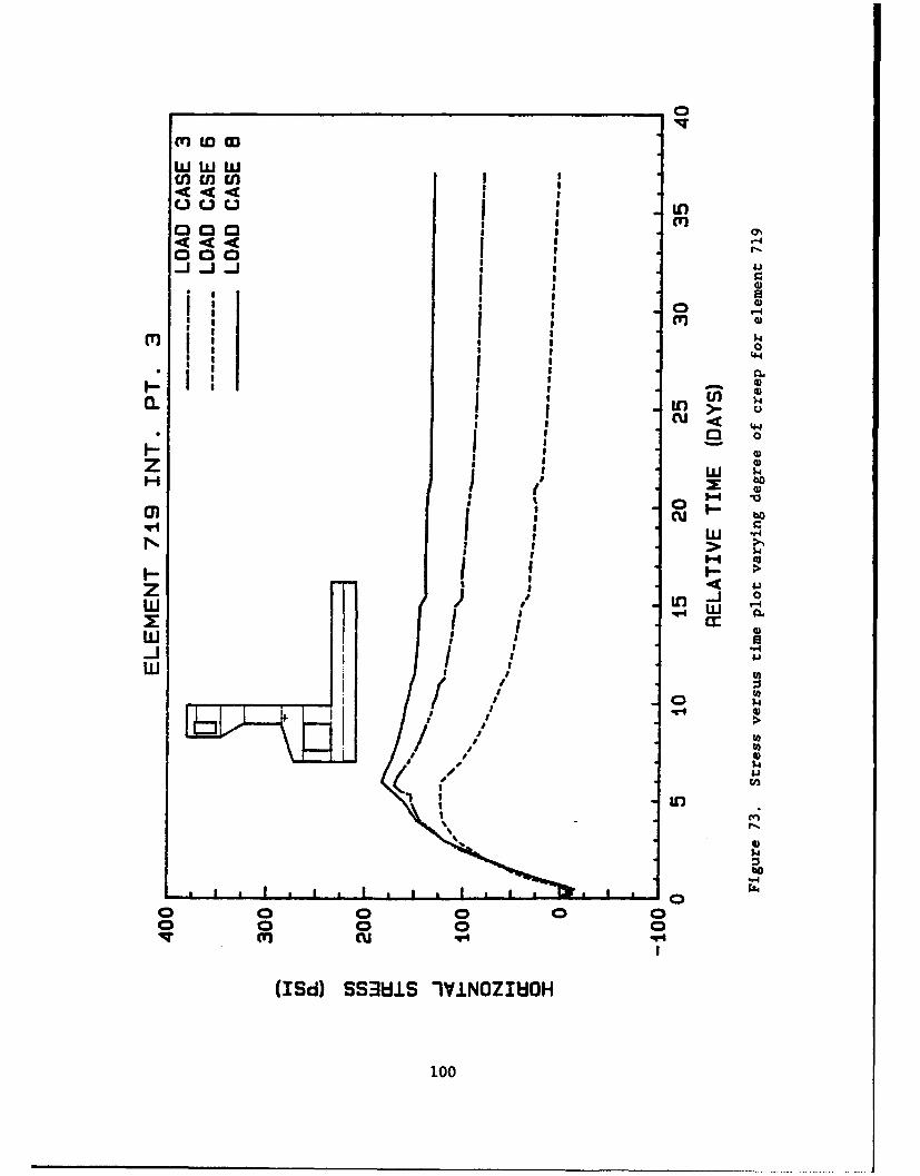
by a new lift--for example, element 719 in Figure 59--the band on the shrink-
age plot formed by the different load cases is wider than for the elements
that are at an exposed surface--for example, element 705 in Figure 58 (with
the exception of Figures 52 and 55).
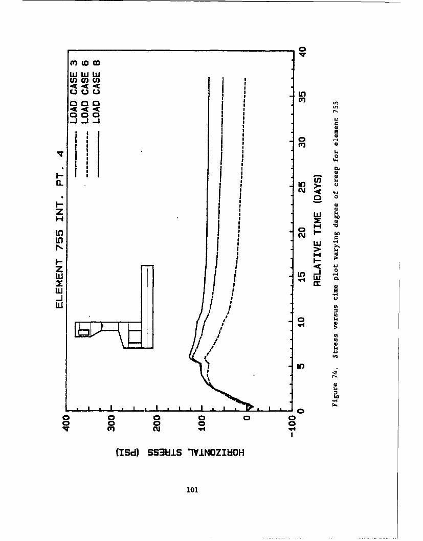
Effect of Creep on Resulting Stresses
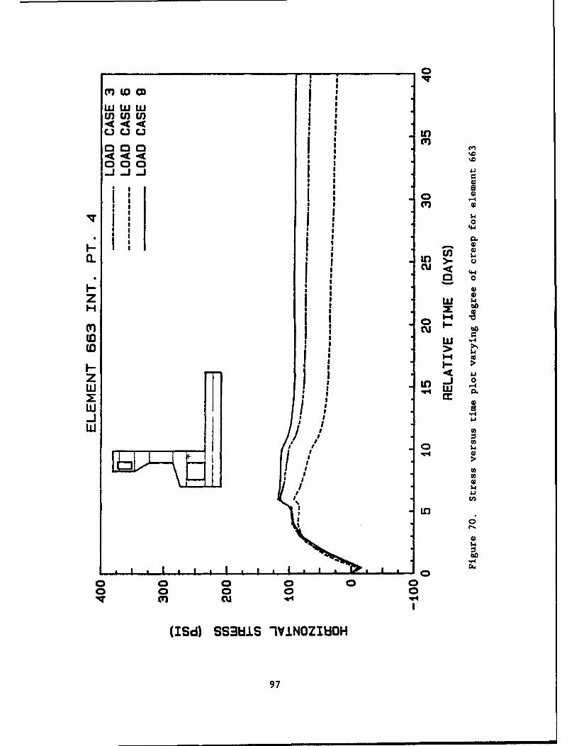
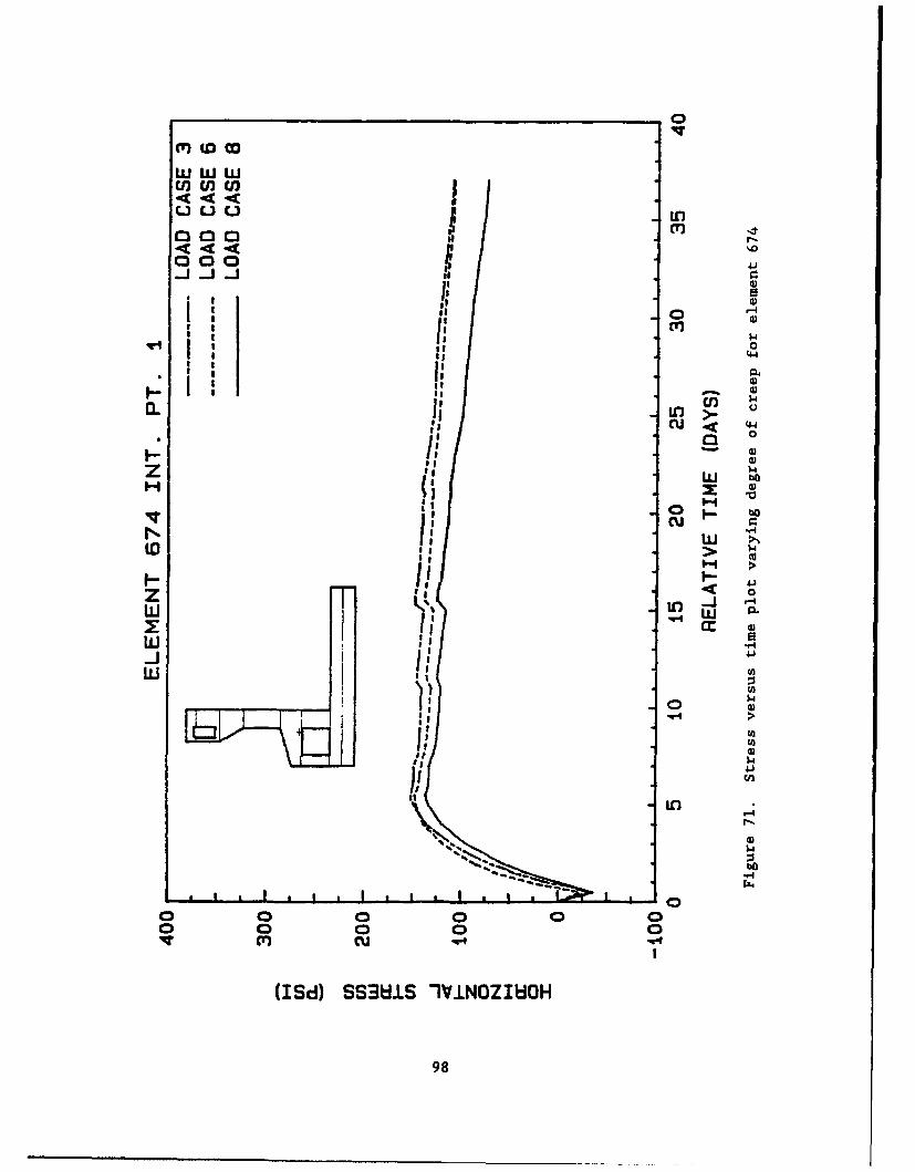
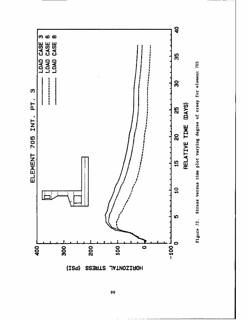
69. Figures 66-79 show the results sf the analyses with shrinkage fixed
at the lower bound value and varying creep. Observing from the figures, creep
tends to relax the structure except near the center-line support and at loca-
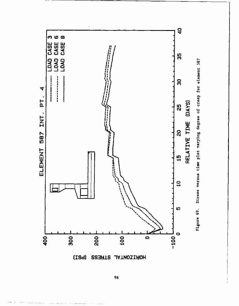
tions where the multipoint constraint is applied (Figure 69 and Figures 71 and
75). These results are expected and justifiable.
70. In small concrete members, creep tends to produce higher stresses
since larger deformations will result. Consequently, the stresses also will
increase since the stress is proportional to deflection (Fintel 1974). In
mass concrete structures, however, large deformations are usually not a major
consideration, except for deformations related to settlement. Thus, viscous
flow of the material due to creep will work to relieve stresses or place the
structure in a more stable state of stress.
92
00qI
000
444 4000
U)-In>u -C
0 44
0~0
14)I-I I 0H I '.
1. 0uI-o Ow
I Cu w 01
Ir.
IiI
w 93
'~camcoo
000 ILInLA
m r4
* ~0'.
4.4
a1 0
Ln w
In Iw 0
r 0.w 4)
I ~~4.U
I I o Ln
% % %
Cu 94
en w c
IL I-Iw
Il U3U00 I.
* II 0
0.. I in 4)>-U
w pt-4
U3 wiidz dw
x aa
100
/Id 4SWI IVI-IH
95.
m (D 0
000 cn) U
000 4!
0 0
CV) 0
ii UW 5
I- 04
If 0
z IsI4w
14
w4'MM
I)4
ILr
p% .. bo
(ISd) SS38LLS IVJ.NOZIHOH-
96
wWWLLJ I
000.4J~ < -it1-
0
0 o
I I I.- $4
14)
W 4W
w w
I ~4.
W 0/
IV m cu
'Id 0S I I-iNZIIO
97
000 cr)
000~J~J~J 'a
0
fl4
CU<
(a
z '
CCN !
(.01 4 )
0)
Lr))
bO
(ISd) SS38IS 1IVINOZhIEOH
98
0
cv to
cna u)
a4 ii 0 t
000 1~J~I~J I4-)
Ii 0
* 0
H~ bI* I: C4)
Icu bow 54
z I: 4w i
w//I; U)
>~.
I 0O
L~vEI~iJ //T / cu
(I~d)SMIS-IVINZIW)
990
cn in 0cr1wow
000 Ia cw000
I 0
I I0 0
w "I> >I
z < 00
N a
I I U
I 41
<K In
(Id 0 0 0s
(d)SS3W.S 1YVINOZhIEOH
100
-0
LiLU LUI
C.)C.U) En I
0 0 -4
1 0
a I (I) 0.
D 0
3u W
* I0 0
LU.
of a I -, b
In I
J* 0 I- 4~
Ii 0IV m I
1012
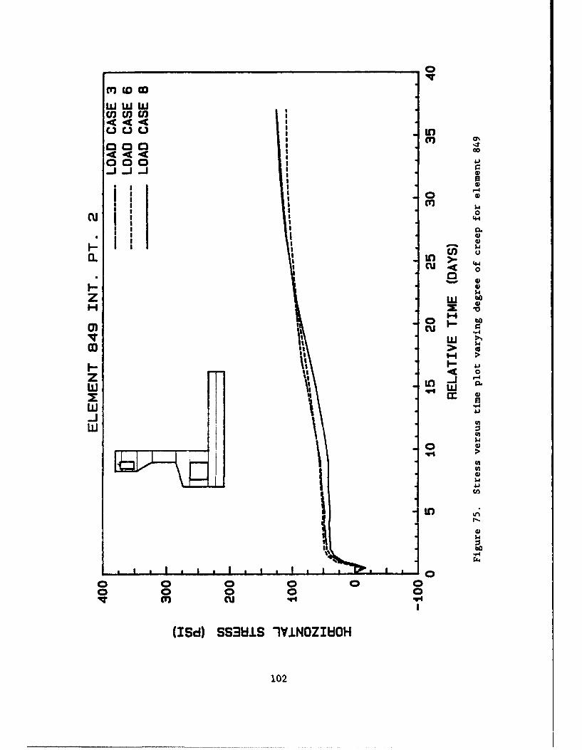
u cn cn
000000 .
~ I 0inI0
cuj o
x 10
I 0o
z- I- -z _ bj r
w- w CL
01~c 0g. )
LI w S4.'-J4
LU))
1.)
100
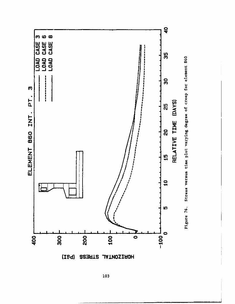
~ Il 0
U U C. Cr)
000 0
to 0
CIJ4 )U) Q
I% gc 0
I- a$0
co a> to.-.
ZL Lo .
I I I of~W '9 0-J ii 4>
/ 0a-a
103
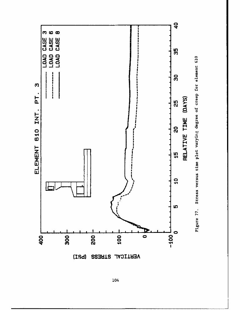
uw w w
0004II~ IC 4
Cl,''
0 44* C)
to >P >.,
I I-
z 0w * -LI
-4JLUO
% %)
0104
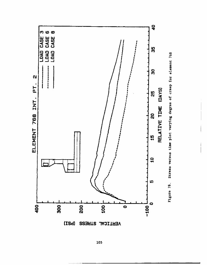
L)C.)C J L)
000 j0
cu 3 4
0
ii . 4.4.
C 0
N w5- (x
z 41)
LU,
100
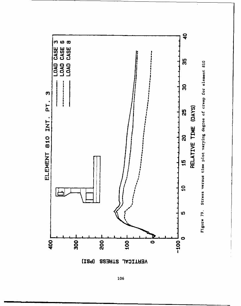
m ID w
CC.3C ui u10000 co000 4.
0
'4)
a.) >. 4aU 0
Z I w
w 4)
Z a 0
w 02
aL I q-
%. -
0 0
0 0
100
71. Looking at the specific creep curve in Figure 16 we can notice that
creep will start to effect the stresses in the concrete within 2 days after
the material is placed. From the results, it can observed that the effect of
creep is mostly obtained in the first 15 days. Thus, short-term and
intermediate-term creep has the greatest effect on the tensile stresses.
72. As was the case with shrinkage, the results shown in Figure 69, 71
and 75 indicate that creep also has an effect of increasing the stresses at
these locations. This is related to viscous flow causing the element to move
away from the support but the support restrains it, consequently producing
higher tensile stresses. After the support is removed (7 days after the lift
is placed), the stress pattern for the load cases returns to the same as in
the majority of the figures (i.e. load case 8, no creep, produces the highest
stresses, followed by load case 3, lower bound creep and finally load case 6,
upper bound creep) (Figure 75).
Combined Effect of Creep and Shrinkage
73. The results for the four load cases with creep and shrinkage varied
among the upper and lower bound parameters and for the load case with creep
and shrinkage neglected are shown in Figure 80-93. The results show that load
cases 3 and 5 and load cases 4 and 6 are narrowly banded. This indicates that
creep has a more pronounced effect on the tensile stresses when the given
shrinkage function is used.
74. The results also show that neglecting creep and shrinkage will give
conservative results for most of the locations investigated. In addition,
elements 561, 719, and 755 show the stresses still increasing after 30 days
when creep and shrinkage effects are neglected; whereas, if shrinkage and
creep is included, the stresses are fairly stable by this time. Looking back
to the previous figures, this is not noticeable. Thus, the increases with
time appear to be related to both shrinkage and creep being neglected. How-
ever, shrinkage is more of the cause since, as discussed previously, the creep
function used does not have much of a long-term effect; whereas, from the
shrinkage plot in Figure 15, the shrinkage strains are still increasing after
40 days. Thus, including shrinkage will produce stress relaxation but without
shrinkage, a tensile stress increase occurs due to the increasing Young's
modulus and thermal cooling which causes the element to shrink.
107
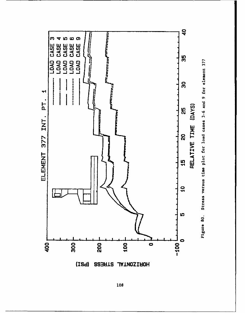
00000
cnccou 54
0
C3)
I-I U
'-4
~-g 0F- 44- *
z 41.'_j0
I )I LE) r
"4.
LLID04
o 00 0m cu
(ISd) SS3W.S 1IY.NOZIWGIH
108
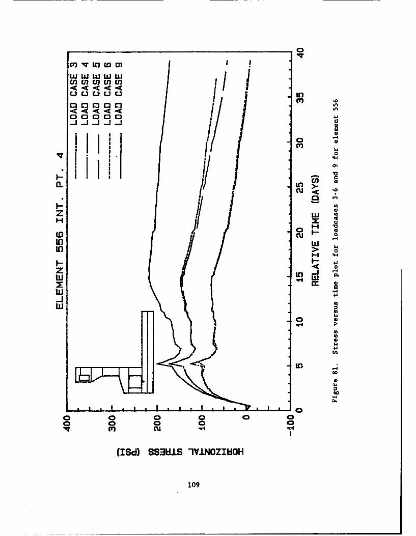
00000
cn IVI oc
crU)
641
0'
z III.- *
IDd
0.
w U)
-J
If))00
0109
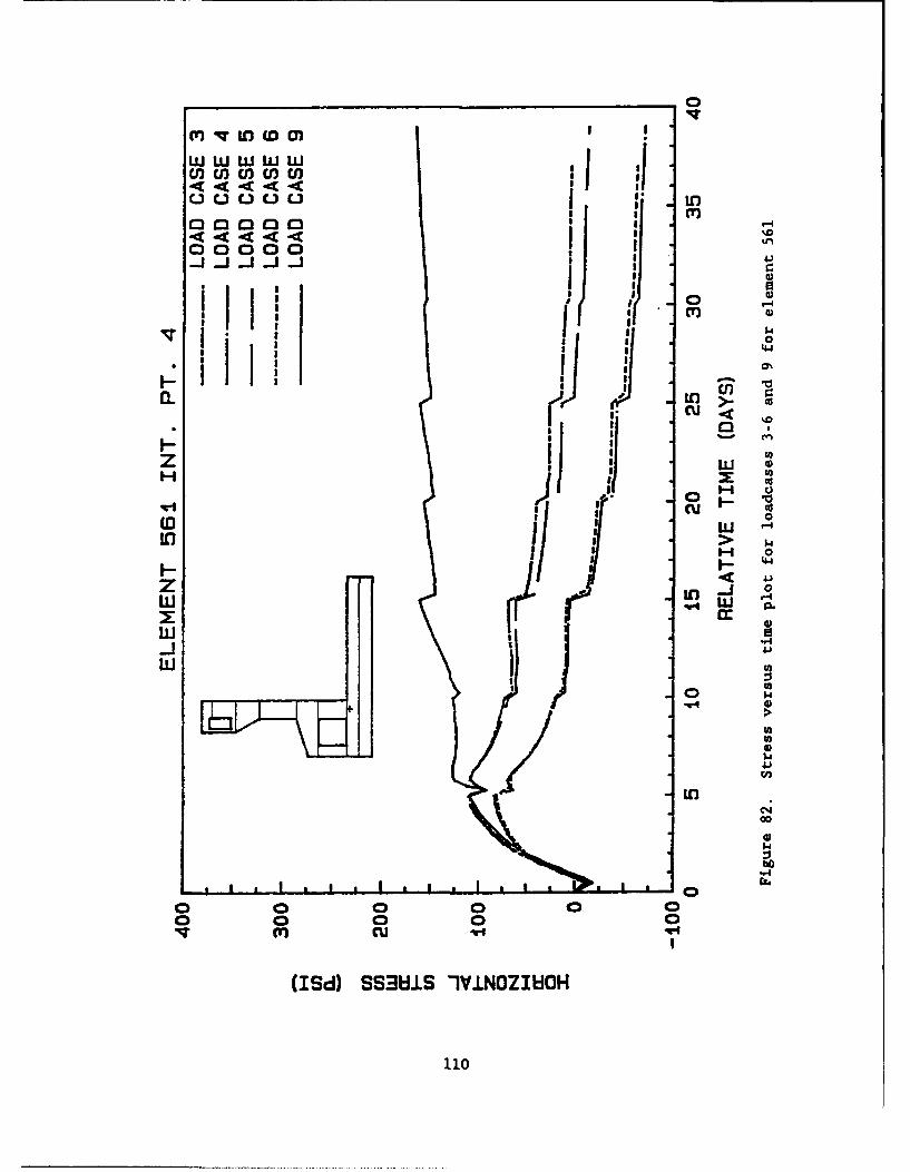
I ~ 0
I 4
I I UI I *S ID
a 4.1
. Lr ) >- c
cu Cuw0-
II 0
F- 44
z -L1J tailCc 4
0C
II
(ISd) SSMIS 1Y.LNOZIHOH
110
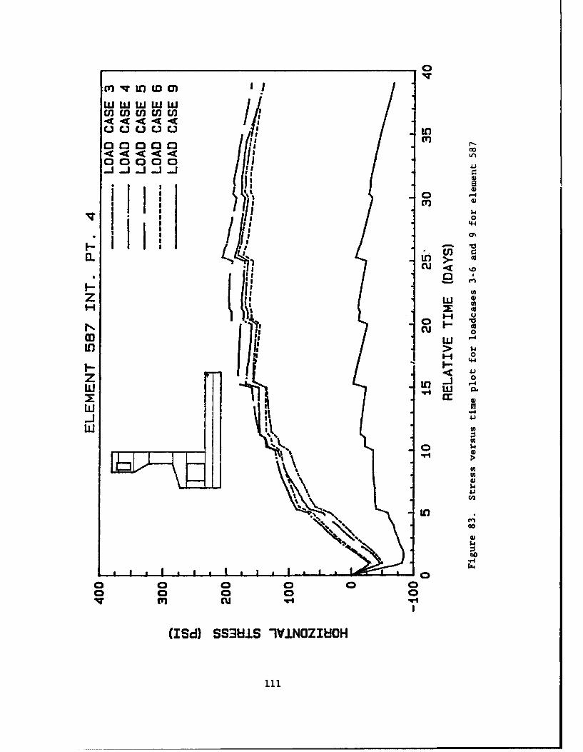
00000 0i I
4j
044I
U)
0f) I>- cocuJ
iiI 02
34 0
"r4
4.3
w I
.q.4
00
00 0 00
(ISd) SSMI±S 1IVINOZIE!OH
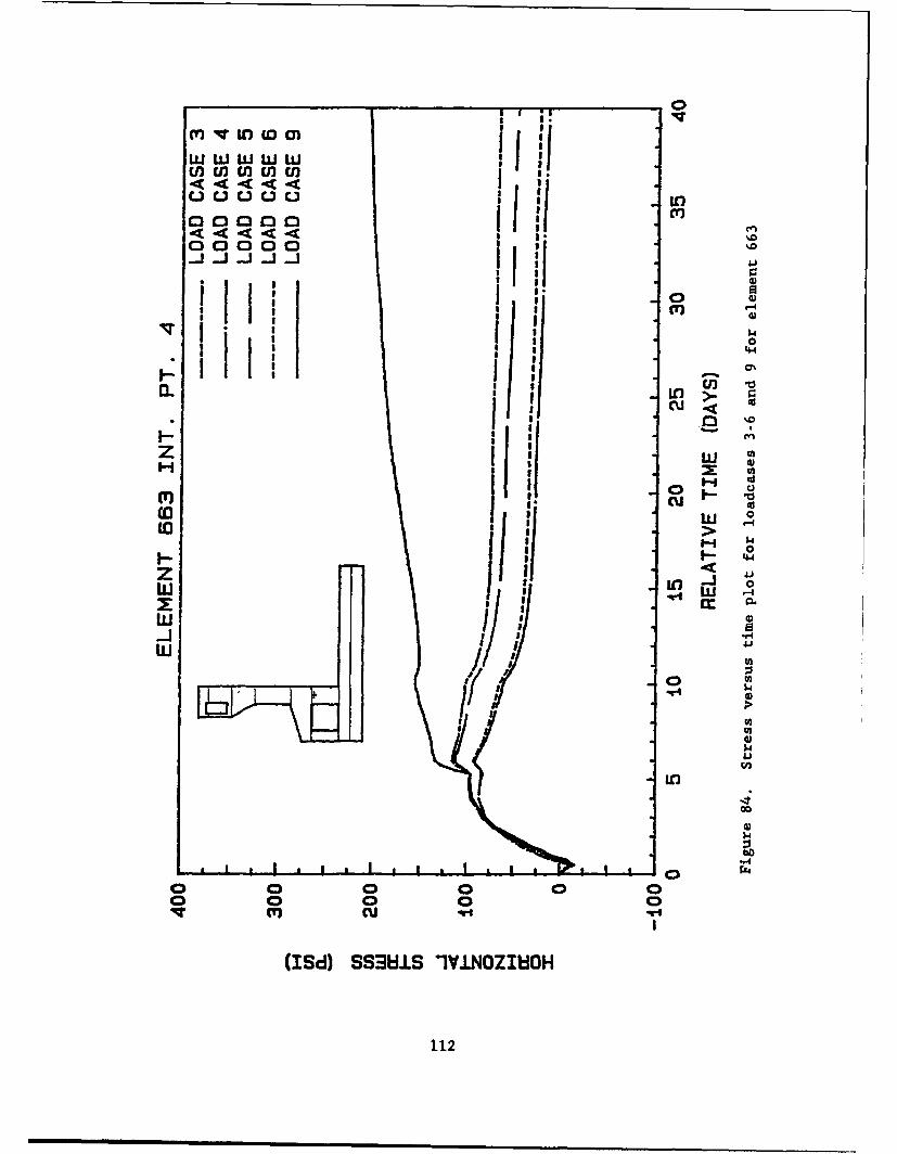
in C V u) in in iC.) D 11 C. l 0,f
* 3 01 '~4-
I* LO>C3J
1- I cv
(0 I I
a a 03 ~4.
x cr
w
0 a,004
1122
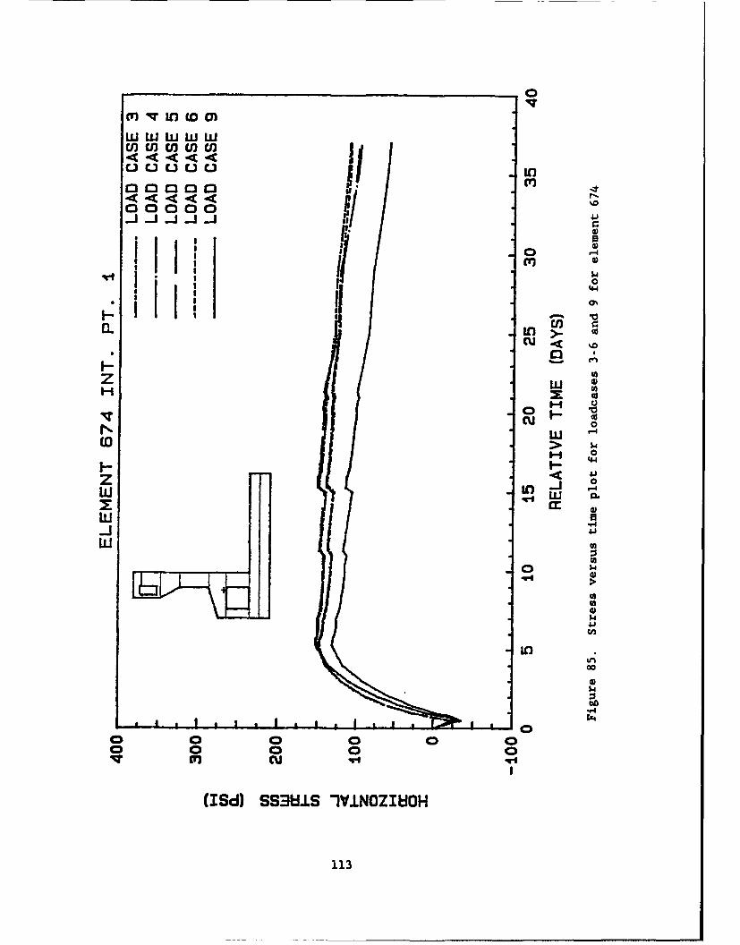
(I) qqLO co 01
Zncnmncnn u11u< -< -< < -100000 )L L) (In
0
L.- > -i co
cu 0
0S0-4.
z 41w C7- ~cr-4wa
I ~4-
w CA
LI%-\4f Sa'l IVNZlO113'

0
W LLJ W wwu) ncnncn u) u
00000 IjS
00000 IIu0
CI,
In 0
o c/Ii 14-40
'I 44z ii tn-Johi 0 1 I 0IV nc
(Id S I iYNZEO /144
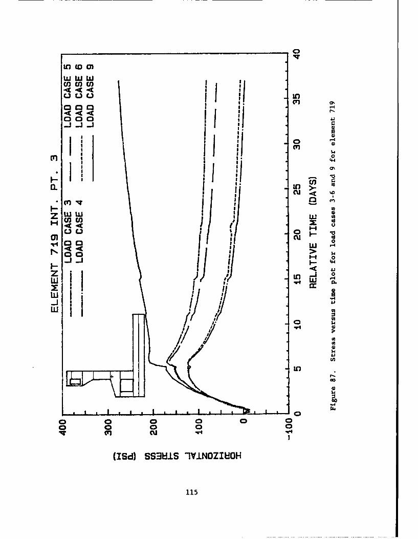
U) ci) U)
C. ) )F) 0
41
o0c"
cu--mw Iq w a
O)U)U w
U C.3ui sr4
00 0
WH 411In -
Z4)
0 l 00F
115
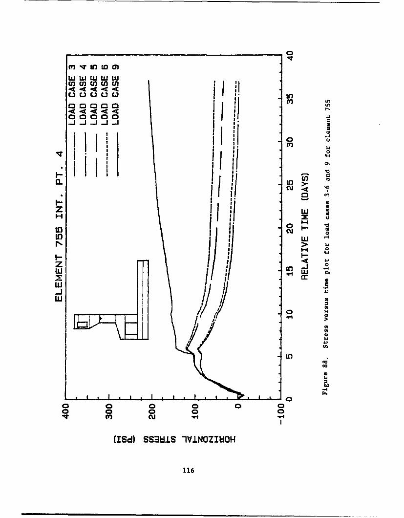
m~ IV to
w~~ w W ii
C.3 C.) L) C) C.Af~~In
-4
0 0I' I 44
1111 liiCL iiac II Ii '.
0 ~1-4 4,
z I IQIi 3.0
I 1-4
NG Ic
I~0U.74
-Ju
wId SU IIOIO
1164
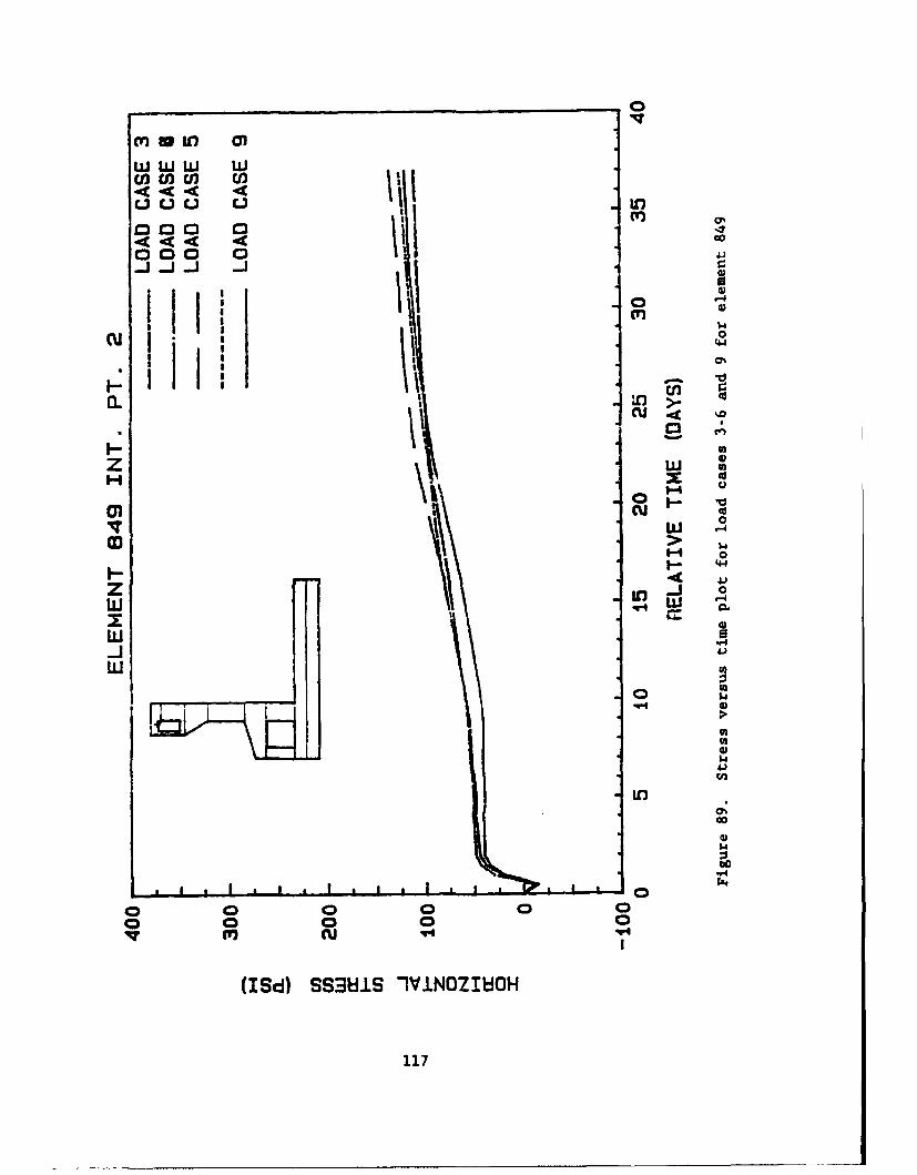
w ww wEnCfl lU EflI -C
000 0 i000 0 1
in 0
U,
IV w 0
x Iz
LI-
041LC)'-
Go
S-I
H"
cuU
(I~d)SS3HS -I.LNOIEI0
LU117
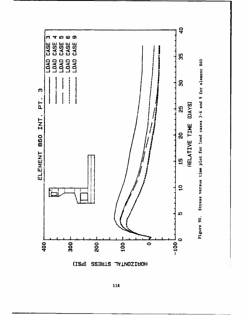
m' IVCr D 0)
in ' in 0) 0rin
co 00
a. i
0" 0 '
w 0@
co > -.
'.4
44.4
z 41 II' Er) 0LU II III
CC
Ii:1 '
1 41
(
(ISd) 0SHS-VIOIO
118
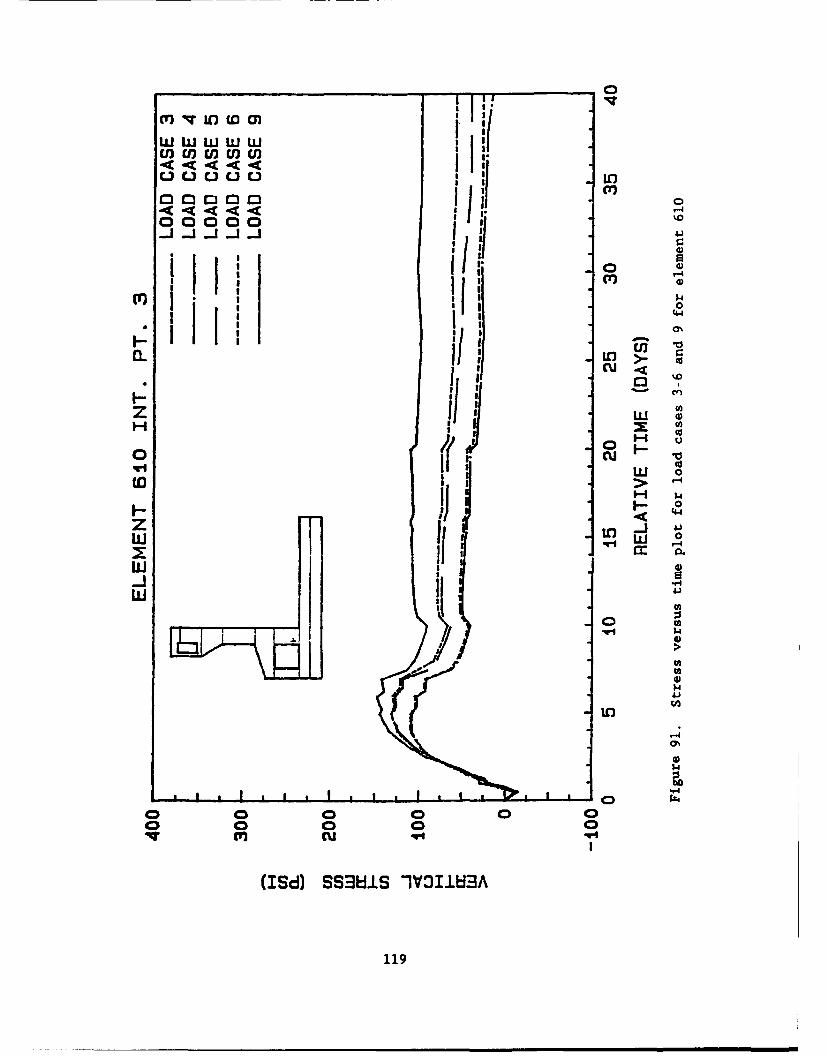
M' ID Cr D 0)
u) cn incin uI
00000
Hir 40
CL~
I-Io 0
F- I-
.Y~w4w 8 0
Jr -Jt4w 1104
.14
'44
1191
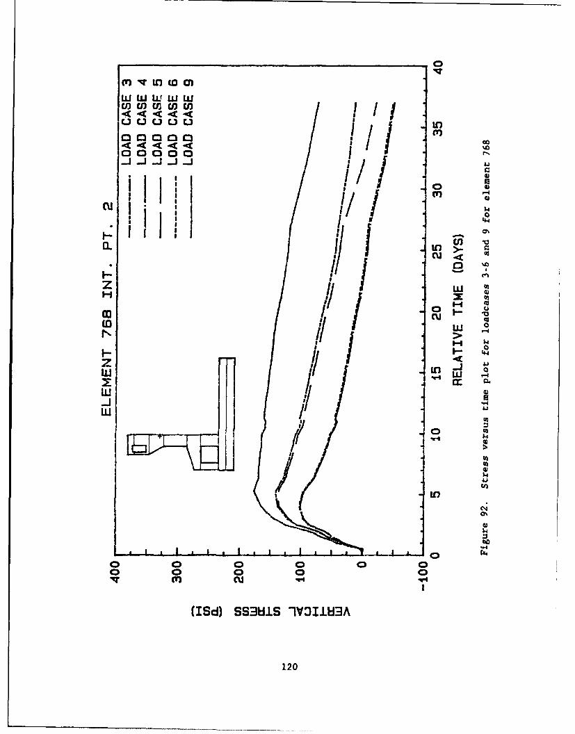
UC.3W2CI3 L) I.
0000 11/ C3C3C300 0 00 1%
a. in U3cu C
* * 11 WIIIV0
C 1 J 'il/ co
w iw0
541
4)
P.4
00
cI) CU *4'
(ISd) SS31d.S 1IVOIJLW3A
120
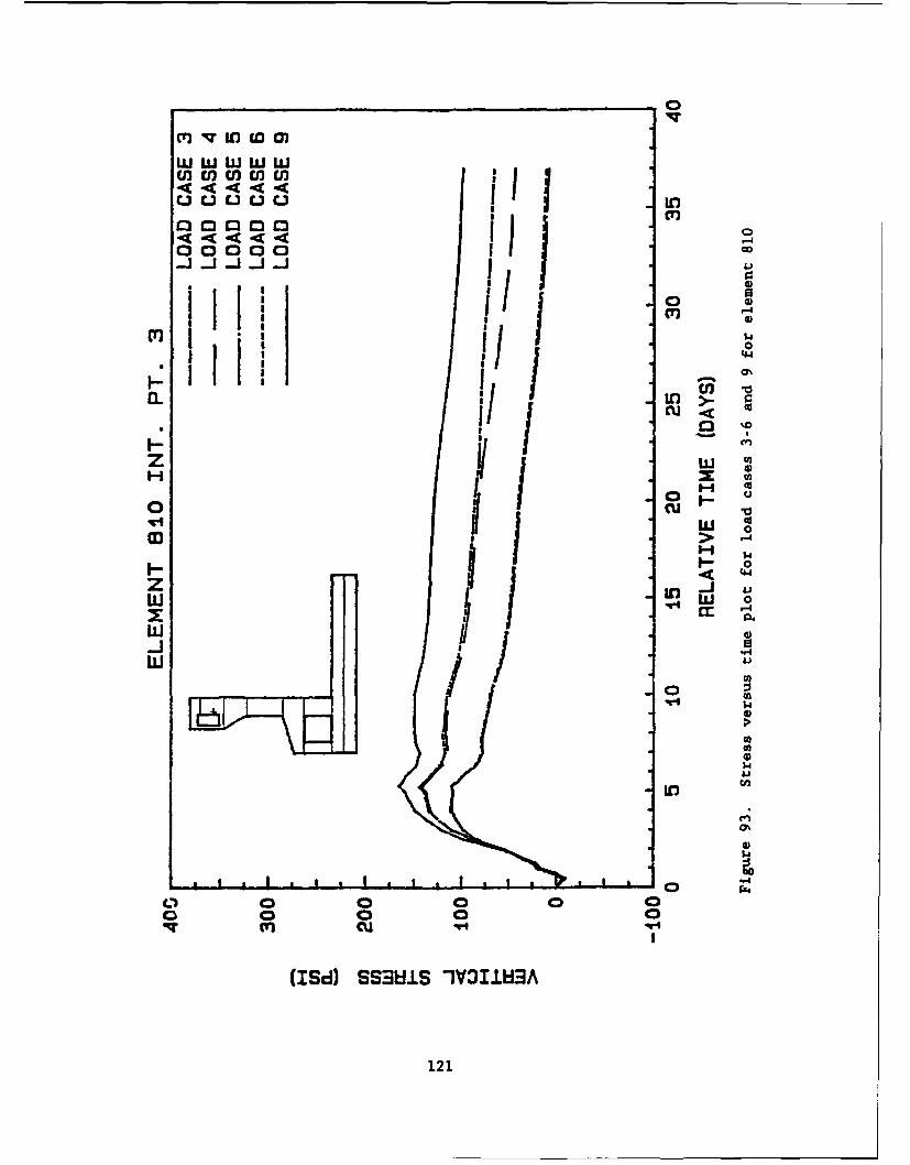
cri~i IVt wa
u5acuc in in ini
030000 I 0
< -C 4-400000 c
3 1 4
iiinz wH X
IIIHo >
z In-LU w 0r
LU 0
wU~Tj
00 0 0 0
CU '4al
(I~d)SSH~S 1V3±~I4
121
Effect of Creep and Shrinkage on Strains
75. As discussed earlier, looking at stresses alone would not be suffi-
cient in assessing the significance of the response on the structure when
performing a parametric thermal analysis of mass concrete. Also, since the
cracking criterion used is both stress and strain driven (see Appendix A), the
strains as a function of time will also be presented for load case 3
through 6.
76. Figures 94-107 show the strains plotted against time at the same
locations as previously examined. A common pattern exists among all of the
plots. Initially, after the lift is placed, the strains are positive since
the heat added causes the element to expand. At approximately 2 days, the
strain starts to decrease due to shrinkage and subsequent cooling. In most
cases, the strains become negative since shrinkage and thermal cooling cause
the structure to "shrink." For the elements that become embedded under a new
lift, (Figures 96, 98, 101 and 102) at 5 days, the strains increase again due
to more heat being added to the element.
77. For these realistic load cases, the strains never exceeded
100 micro-strains, a value commonly used by the Corps for predicting when
cracking need be considered. However, for element 768, integration point 2,
the strains for load case 3 did reach 93.7 micro-strains at 2 days after the
lift was placed.
78. A similar pattern is again evident for which load cases produce
higher strains consistently. Load case 3 generally produces higher strains
from the time period examined. A similar banding also occurs for the strains
except, now, load cases 3 and 6 are narrowly banded as are load cases 4 and 5.
This type of banding should occur since creep is stress dependent (see Equa-
tion 5-3); whereas, shrinkage is strain dependent. Consequently, from a
theoretical stand-point, there should not be a difference between load cases 3
and 6 where shrinkage is constant and creep is varied and similarly for load
cases 4 and 5. In Figures 99 and 100, this is what does occur.
79. Based on the previous results, load case 3 was selected for further
investigation. First, all the locations where the horizontal and vertical
stresses exceeded a specified value were found for each time increment. In
addition, since load case 3 consistently produced higher tensile stresses, it
122
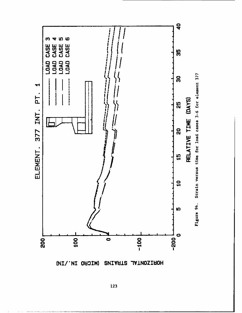
zw w w I'
0000
I I II'll r) cv"I I I il 4.
I I eli,3
- 1--.
03
F-- 40zm
<1 q4
/ 0
0 0
cu V4 q4CUI I
(NI/*N1 OtHOIN) SNIYW.S IV.LNOZIMOH
123
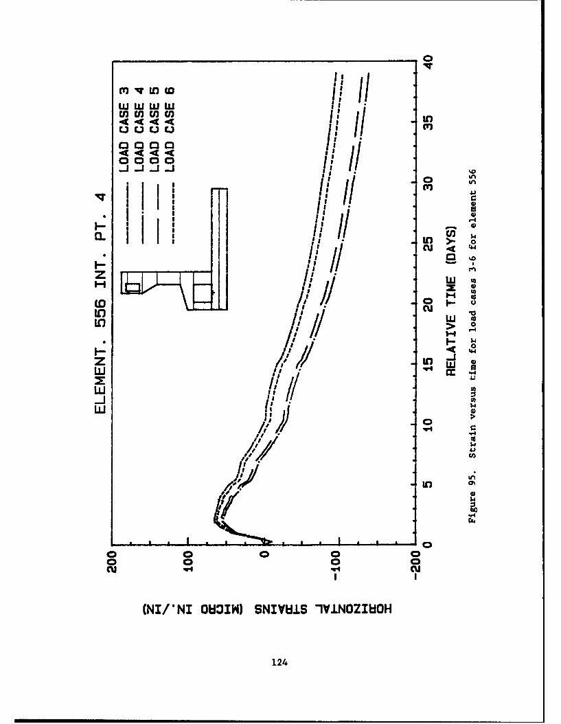
____ ___ ___ ___ ___ ___ ___ ___ 0
m~I .1Lr (II w w
0000 1/it 0 U,
Iiin
Iu, >-I oiI'!u 41
C3j.* liii 0%
to Ell
in Cu
/O 0
W14)00
1/',"ff 4)$4'. U,>
"-I
0
I I
(NI/ NI ONfOIN) SNIYW..S 1VINOZIldOH
124
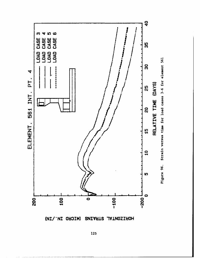
cn qqLn 0
U IL)U U n
0000 1-4
a.~H I U)
I-4
H c'J(0 1(1
1-4 0
1- 4z 1/
14)
Ii >
(NI/*N1 OHOIN) SNIVW.S IY±NOZhIMOH
125
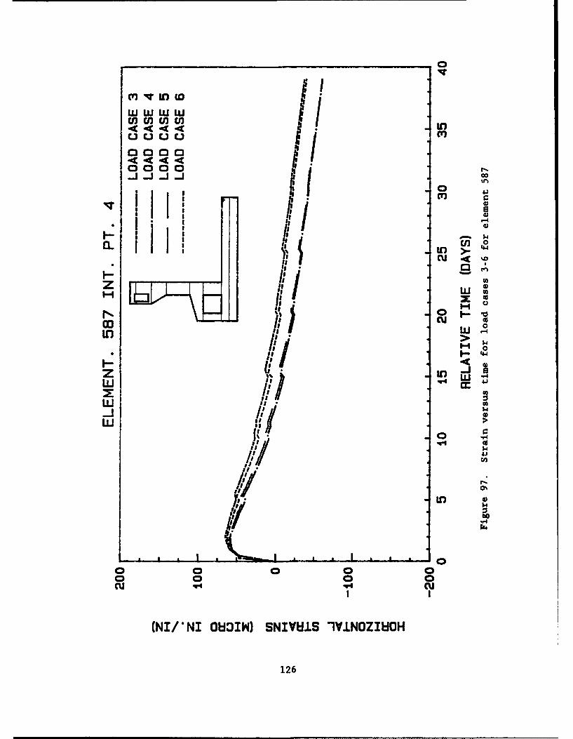
fi Iq n
0000
lii cv,
1- . 3 446
zo 0
ww
I,, 0w 141
'4'41.4
u~i 0
1a4
(NI! NI IONI) SNIVW.S IV.LNOZIEIOH
126
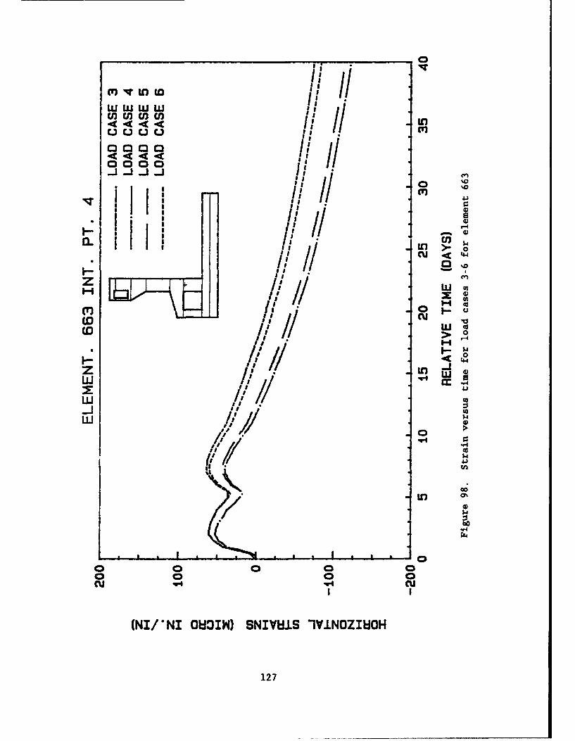
ET) Iq Lno to Iw w ww fitIi Ii InU 1-L0000 ii0000 I
~1~J~j~oil0
*r4)Hoil ii40 L
> 0
z Iiww mI
/oill
LbU
d ~4.
U) 0
114
(NI/ NI OldOIW) SNIVW.S 1YVINOZIEIOH
127
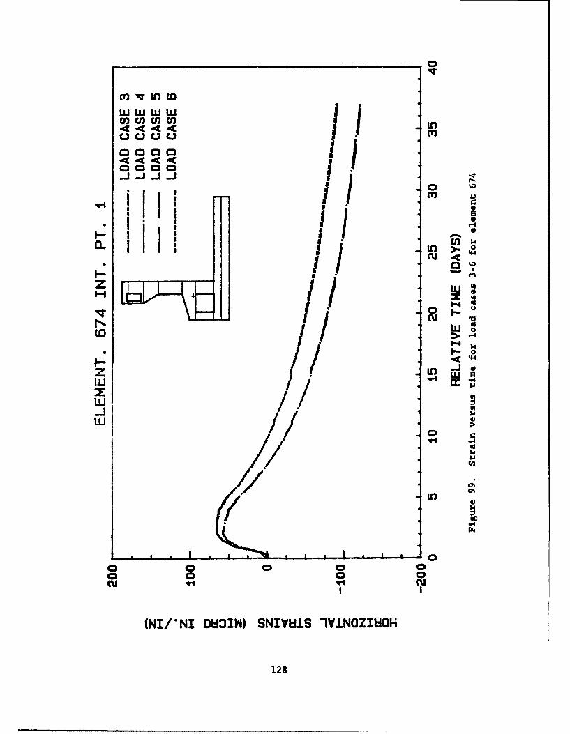
U) cn nU) U)
0000 3
53) 0
F- 4,I Ia. ill!F31
II 0o(D > r C.
z1tr-It 0 r "4
0 9
t 0
0000 0 0Cucu -w4 4c
I I
(NI/*NI 01:10Th) SNIVHLS IVLNOZIH:OH
128
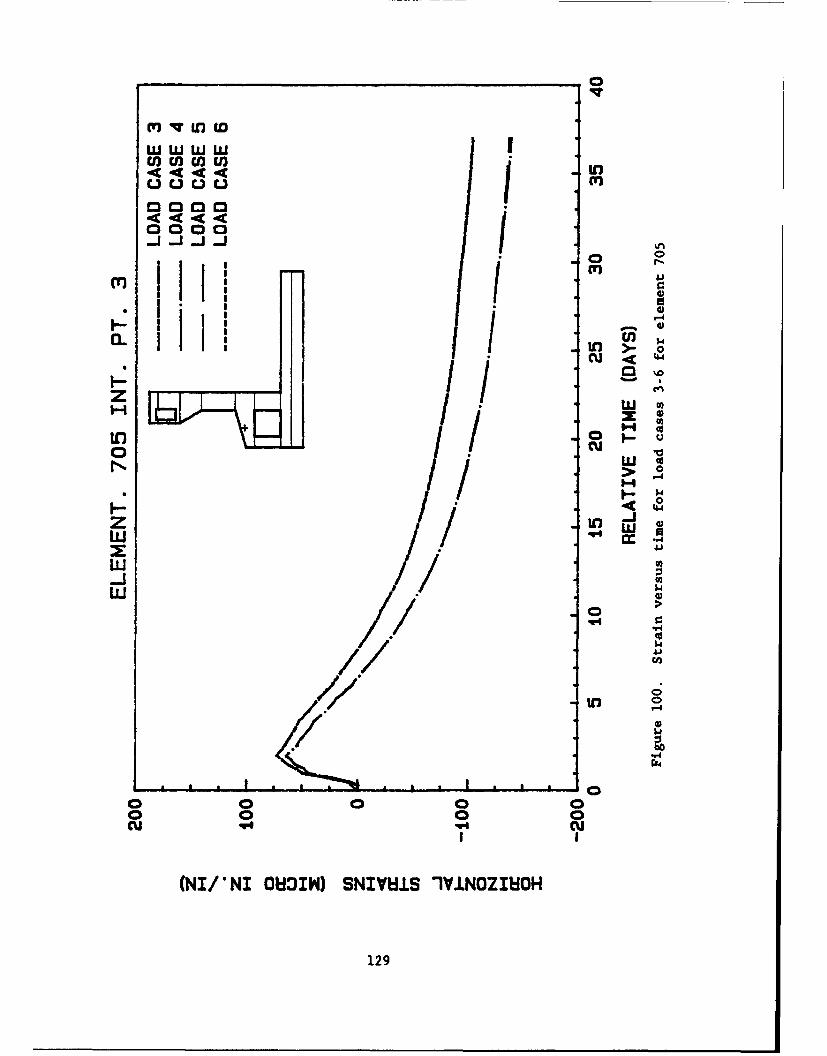
wwwI I)toJ
unncc IL
0000
0111 Cr
I W
LU
ii >0
Wi'4 .-.a
0 JJ
".40
Lu V40
(Nl*Nl0M3W) NIVIS IVIOZ~d 0
7/129**4
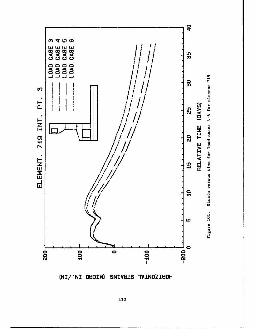
0000 1
(n IJ Jr J IDw. w -4uI u) n u
*IIT)
Coco 1
I-C /C 4 .4 0i
"-1 - -j O1 r
N 0DI, II I 44
w 0
// In
cr.
1/"4 '4
ml11/7
0 '4
cu V4 cu
(NI/ NI OMOIN) SNIVEI1S IVJ.NOZI~dOH
130
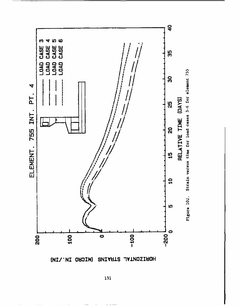
m IT 1r)
L)C.)C.)CU lot
0000 L
I, cr)
Iii:i 44 i
IH co
w r
0S.
02
LII,
V4 c
(NI! NI OkIWN) SNIVYW.S "1VINOZIWOH
131
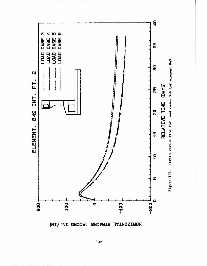
Ui I. I)C c'
CocoCJ0000 :1Go
9099 IIIIII 0lii C'
I- I ft 3-
a. fJ$4,'~i o ,>--
IiL > ,u %
II r
> I 4
3 0
z. Ir L W.4zL (
0 -I
/C54
"g~4
I I
(NI/ NI ONIW) SNIYW.IS "1VJNOZIHIOH
132
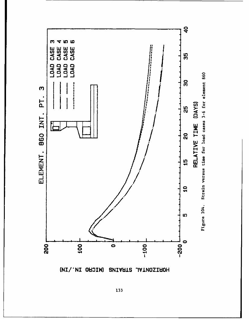
0
000 aq In
0000 1~ II
II 0 41
ii I m
I-. t I'I--* j !cu <%o
35~ 0'
z W ,4
LLJ:
II ý
Z I(NI NI OW )4.)LSIINZEO
133)
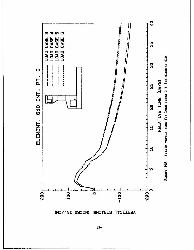
www1w Sf
DI II
cJC)~ I) L) C3cI
0000
'Unn
#- -i-!-
it 0
H c
-j-
LU
0 "0
1' b4
-1-- 0
(NI/*N1 08DIh) SNIVhJ..S 1YIVIIE1A
134
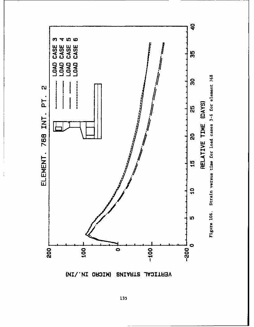
0
LU C.)C. C
0000 /0000
II F0
Cuc <il
* 03
9/, Cfl
zw W-k~1J lii
I,"4I-oZ Ii .4
.44
(NI/*/1 0W).1VEI -III3
135)
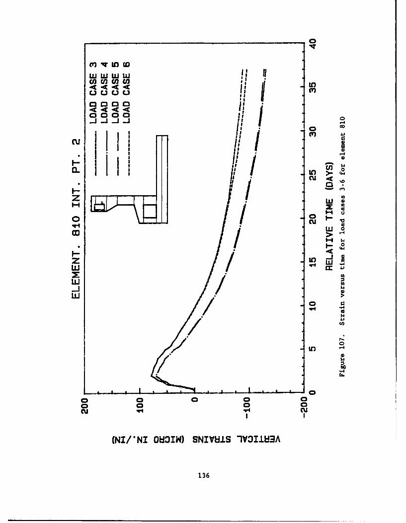
ccccn 'a4' w w
0000I: <
0000 0i~ Ii 0 J5
cu I r
1i- iii 0
w 0.co r
z If I',w Ir4
01
I q4
,1 0u /u
(NI/N1 MOMZI SNIVHIS IYOI1GA
136
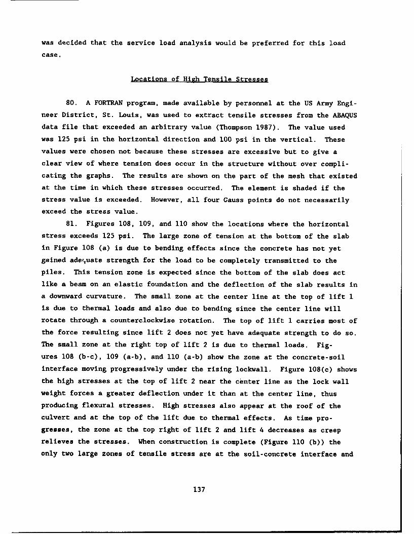
was decided that the service load analysis would be preferred for this load
case.
Locations of High Tensile Stresses
80. A FORTRAN program, made available by personnel at the US Army Engi-
neer District, St. Louis, was used to extract tensile stresses from the ABAQUS
data file that exceeded an arbitrary value (Thompson 1987). The value used
was 125 psi in the horizontal direction and 100 psi in the vertical. These
values were chosen not because these stresses are excessive but to give a
clear view of where tension does occur in the structure without over compli-
cating the graphs. The results are shown on the part of the mesh that existed
at the time in which these stresses occurred. The element is shaded if the
stress value is exceeded. However, all four Gauss points do not necessarily
exceed the stress value.
81. Figures 108, 109, and 110 show the locations where the horizontal
stress exceeds 125 psi. The large zone of tension at the bottom of the slab
in Figure 108 (a) is due to bending effects since the concrete has not yet
gained adequate strength for the load to be completely transmitted to the
piles. This tension zone is expected since the bottom of the slab does act
like a beam on an elastic foundation and the deflection of the slab results in
a downward curvature. The small zone at the center line at the top of lift I
is due to thermal loads and also due to bending since the center line will
rotate through a counterclockwise rotation. The top of lift 1 carries most of
the force resulting since lift 2 does not yet have adequate strength to do so.
The small zone at the right top of lift 2 is due to thermal loads. Fig-
ures 108 (b-c), 109 (a-b), and 110 (a-b) show the zone at the concrete-soil
interface moving progressively under the rising lockwall. Figure 108(c) shows
the high stresses at the top of lift 2 near the center line as the lock wall
weight forces a greater deflection under it than at the center line, thus
producing flexural stresses. High stresses also appear at the roof of the
culvert and at the top of the lift due to thermal effects. As time pro-
gresses, the zone at the top right of lift 2 and lift 4 decreases as creep
relieves the stresses. When construction is complete (Figure 110 (b)) the
only two large zones of tensile stress are at the soil-concrete interface and
137
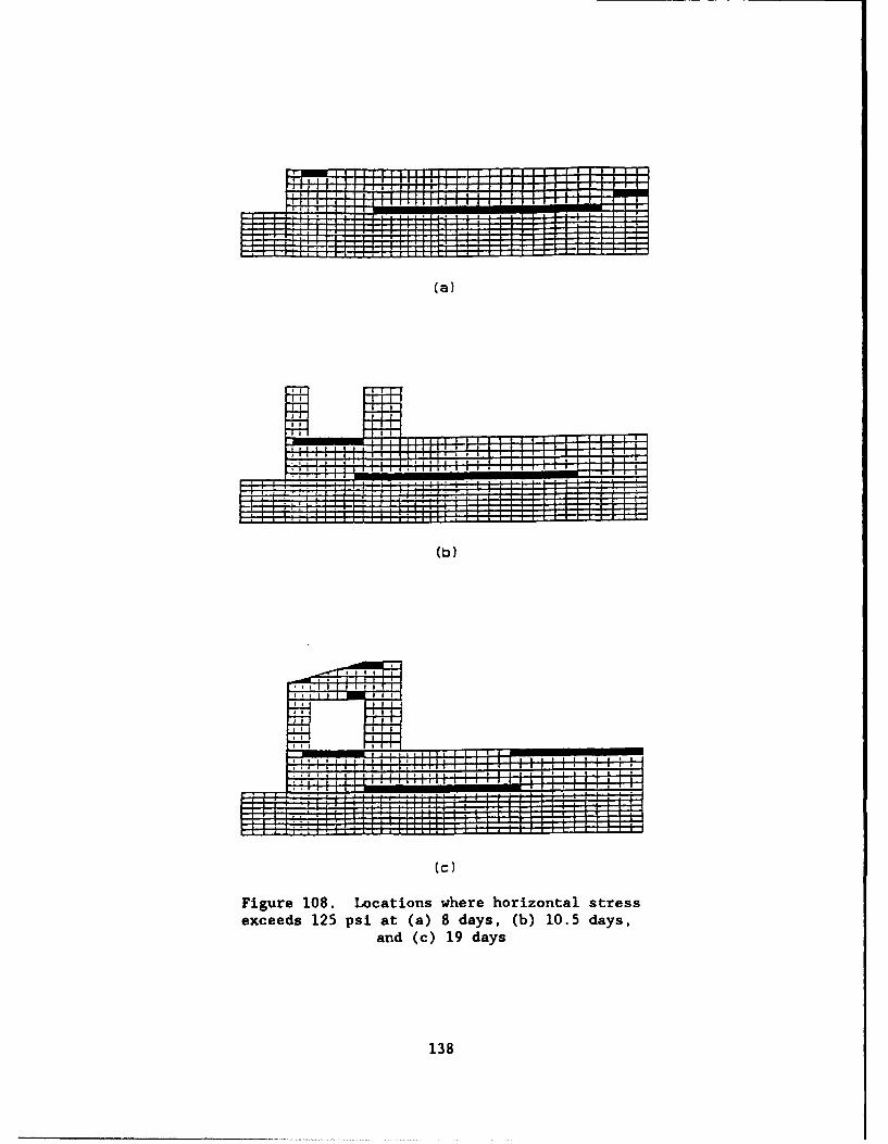
(a)
....... ...(b)
I I I ; ;: i - I , ,
I I i I . . . .'I
(C)
Figure 108. Locations where horizontal stressexceeds 125 psi at (a) 8 days, (b) 10.5 days,
and (c) 19 days
138
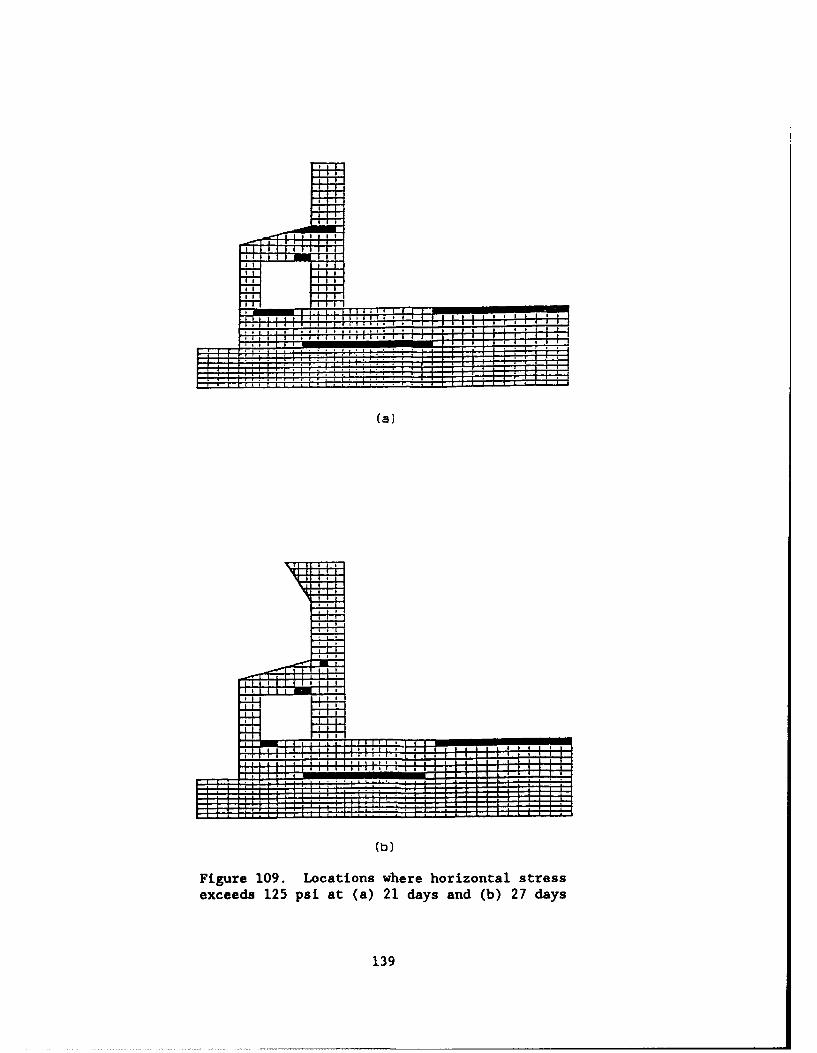
I I .
L, J IJ
.. . .. .. .. . . l I I II I !muL•,:• : I I i: ;- -
(a)
,;I I iIj, ______________,_________I, L I 11IL1
Z13 .......
(b)
Figure 109. Locations where horizontal stressexceeds 125 psi at (a) 21 days and (b) 27 days
139
LI
I . .. . .L I . . .I I, v .. . .i i . . . ' •
(a)
I IN'
!!!L. I! , &- L, ,
*l I IiI I n I
(b)
Figure 110. Locations where horizontal stressexceeds 125 psi at (a) 31 days and
(b) 35.25 days
140
at the center line of the top of lift 2 where primarily flexural stresses
exist.
82. Figures 111, 112, and 113 show the location where vertical stresses
exceed 100 psi. All of the resulting tensile stresses are obviously thermal
induced since, with gravity loads only, the stresses would be compressive.
Note in Figure 111 (b), the 8-ft-wide wall has tensile stresses; whereas,
5-ft-thick wall does not since the heat "build-up" is not as great in the
smaller member. Also note that, as more weight is placed on the structure,
the tensile zones change to compression since the thermal loads cannot contin-
ually keep the stresses in tension as the gravity loads increase--the excep-
tion being near the top of the structure where the eccentric weight produces
bending and tensile stresses on the chamber side of the chamber wall.
Summary
83. The results presented will now be briefly summarized to highlight
the significant findings. First, creep and shrinkage relax the stresses when
only internal restraint exists. At locations where external restraints are
present, creep and shrinkage will produce higher stresses. Most of the strain
plots show an increase in strain due to the thermal loads followed by a
decrease in a exponential fashion due to creep and shrinkage. The locations
where stresses were examined are in zones where stresses were found to be
excessive. Finally, load case 3 produces the highest tensile stresses;
whereas, load case 4 produces the lowest stresses when the effect of both
creep and shrinkage are included in the analysis. The difference in stress in
these two load cases is dependent on the location within the structure; how-
ever, the difference tends to be anywhere from approximately 25 psi up to
80 psi higher for load case 3 over load case 4.
141
(a)
(b)
(C)
Figure 111. Locations where vertical stressexceeds 100 psi at (a) 6 days, (b) 14 days,
and (c) 19 days
142
-I--
I I
1 1 1 1 1 l I iI
III
* II
. . .II+
(b)
Figure 112. Locations where vertical stressexceeds 100 psi at (a) 24 days and
(b) 29 days
143
a a L
144
PART VII: STATIC AND PARAMETRIC SERVICE LOAD ANALYSIS
Introduction
84. Load case 3 was determined from the results in Part VI to be the
worst load case when considering both creep and shrinkage and when investigat-
ing tensile stresses and the corresponding strains. Therefore, load case 3
was selected to be continued to service load conditions. The analysis was
continued for another 72 days after the last lift was placed, allowing the
structure to reach thermal equilibrium and to continue to creep and shrink.
At 102 days from start of construction (67 days from when the last lift was
placed), the service loads shown in Figures 11 and 12 were applied. A static
linear elastic analysis was also performed using these same loads plus the
dead weight of the structure.
85. In addition, the results will be compared with the results of the
parametric analysis of the refined mesh shown in Figure 114. Load case 3 was
again used when performing the analysis. The element dimensions are essen-
tially the same in this mesh as in the previous mesh except at the lift inter-
faces and the exposed surfaces where the element size was set at 1 ft wide in
the direction perpendicular to the exposed surface. The reason for using this
finer mesh was to obtain stresses closer to the surface since this is the
critical location for tensile stresses as shown in Figures 108-113. With this
mesh, stresses were obtained as close as 1.75 in. to the surface; whereas, for
the mesh in Figure 7, the stresses were obtained on the average of 3.5 in.
from the surfaces. The comparison will be made by looking at stress distribu-
tions at critical sections in the monolith. In addition, the pile forces as
determined from a static, linearly elastic analysis of the entire monolith and
the nonlinear incremental construction analysis including thermal loads will
be compared.
Stress Distributions
86. Figures 115-121 show the stress distributions when service loads
are also applied to the structure. Figure 115 shows a stress distribution for
the slab under the culvert. Figure 116 shows a flexural situation combined
with tension resulting from the hydrostatic force on the chamber wall, 0.1 of
145
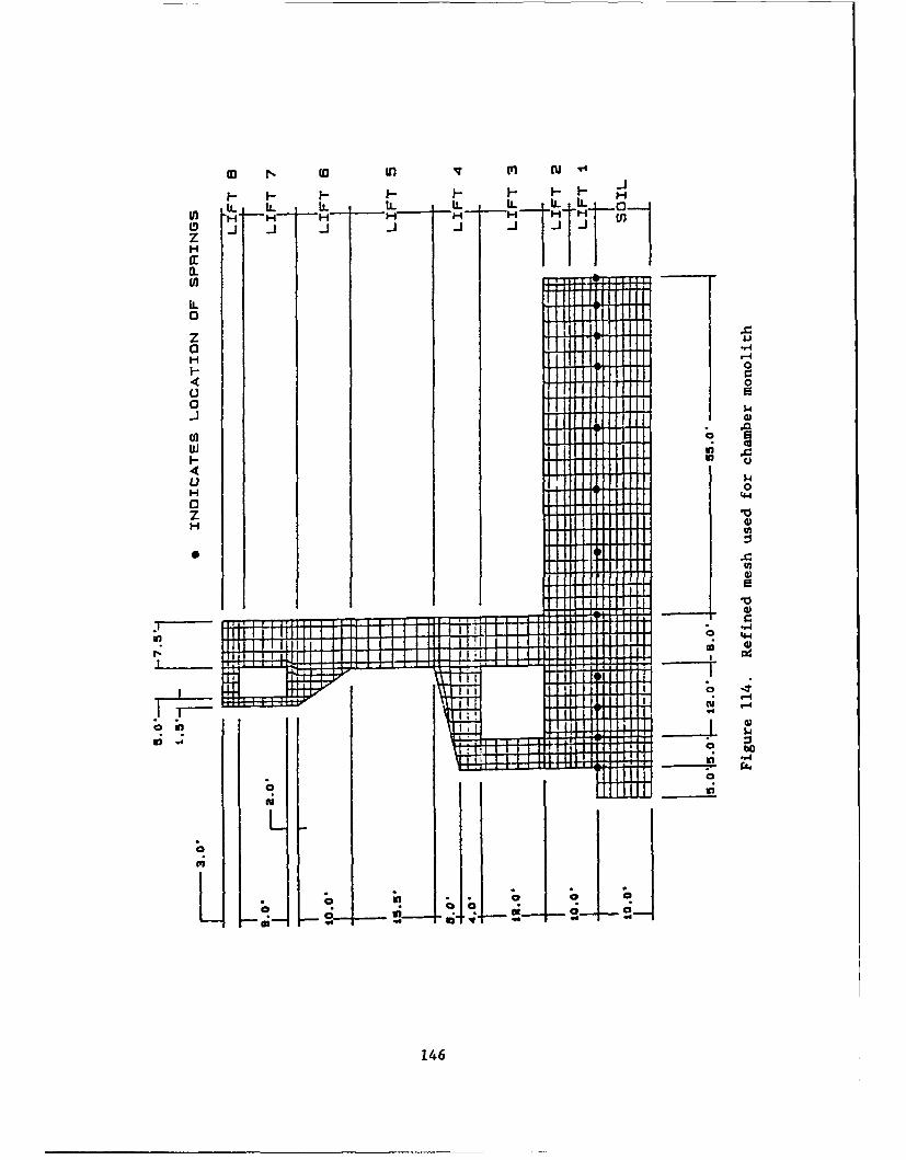
F- 1- 1-F-F- F
in L IL LLL L L L IL
zH
CE
00
4 40 0
ci40-
.0
w
U '-4
z
ZUE)
In -.
1464

LOAD CASE 3
STATIC ANALYSIS
FINE MESH (L. C. 3)
120
too/'
w so
z
S60
40 I
20 1-400 -200 0 200 400
SIGMA X (PSI)
Figure 115. Stress distribution at service loads under culvert
147
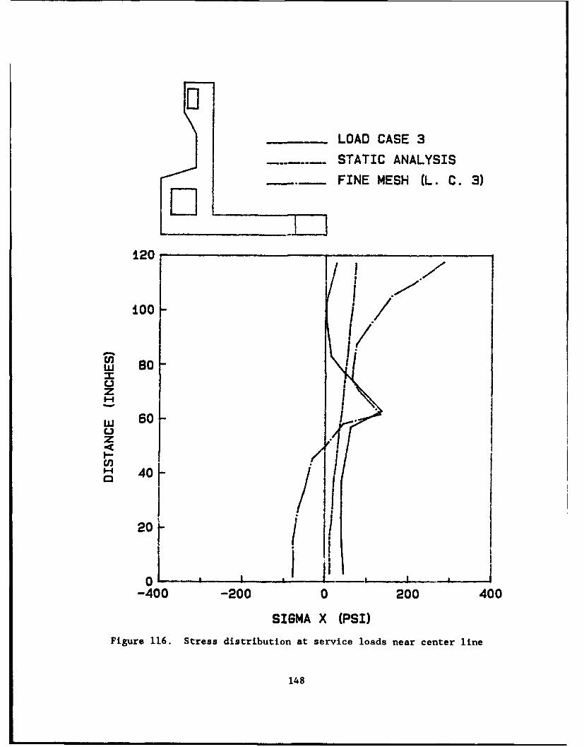
El
LOAD CASE 3
STATIC ANALYSIS
FINE MESH (L. C. 3)D ___
120'1
100 iO0 /
OP.%w 80mz
w 60
zop
'- 40
2 0
-400 -200 0 200 400
SIGMA X (PSI)
Figure 116. Stress distribution at service loads near center line
148
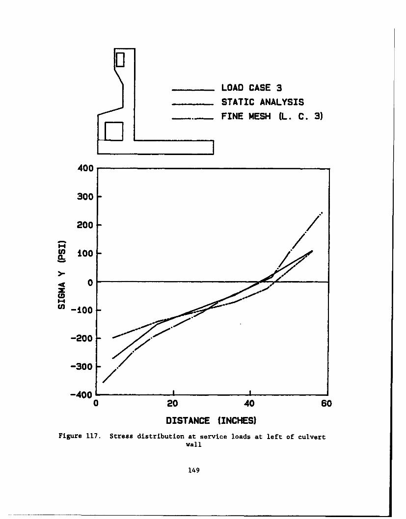
El
LOAD CASE 3
STATIC ANALYSIS
FINE MESH (L. C. 3)
400
300
200 -- /
__ 1000
0
S-noo -
-200-
-300 - /.
-400
0 20 40 60
DISTANCE (INCHES)
Figure 117. Stress distribution at service loads at left of culvertwall
149
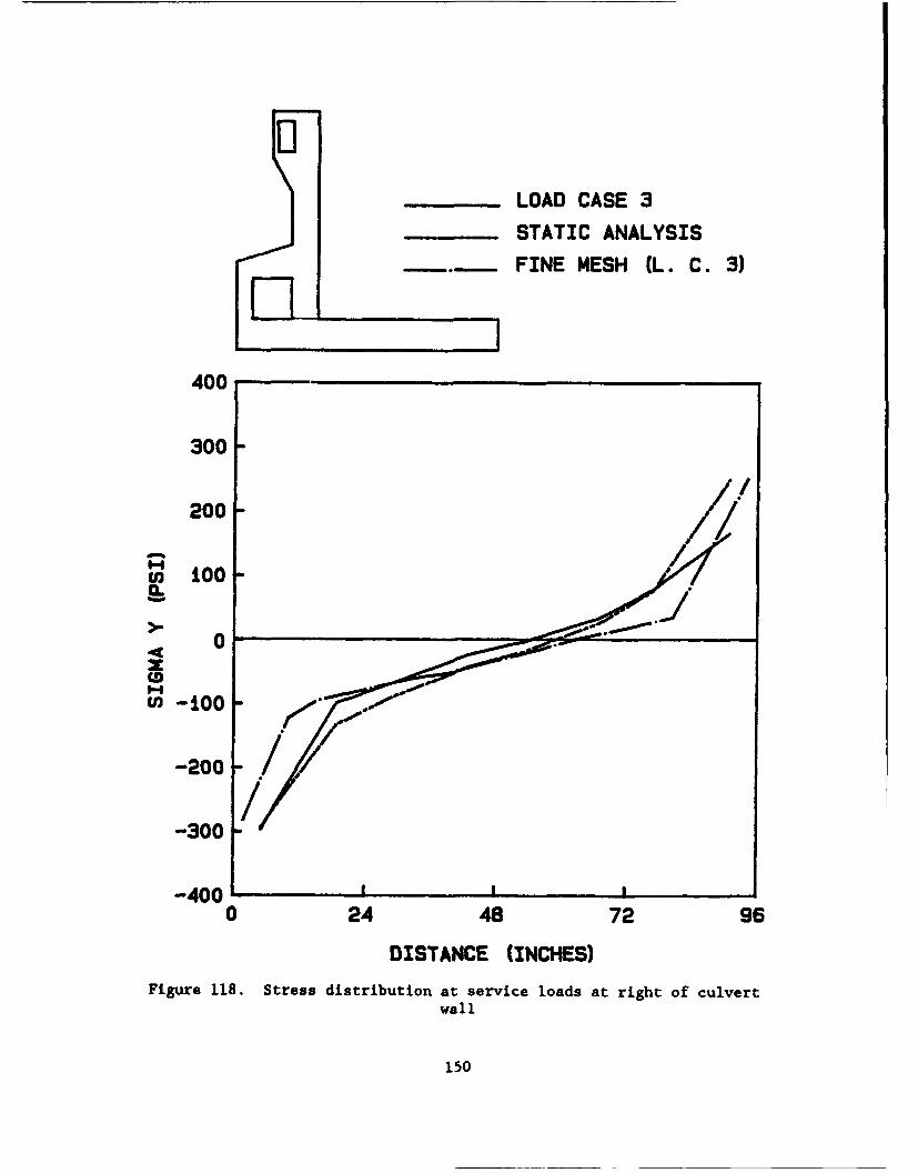
[I
LOAD CASE 3
STATIC ANALYSIS
FINE MESH (L. C. 3)
I
400
300
200 /a ./-200
w-00CL
>- 0
In -100
-300
-4001
0 24 48 72 96
DISTANCE (INCHES)
Figure 118. Stress distribution at service loads at right of culvertwall
150
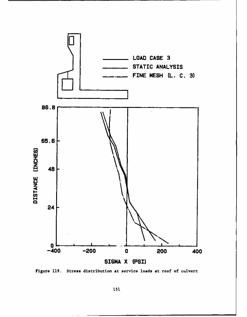
LOAD CASE 3
. STATIC ANALYSIS
FINE MESH (L. C. 3)
86.8 \I
65.6
0-rU
zLU 48
I-z
24
0-400 -200 0 200 400
SIGMA X (PSI)
Figure 119. Stress distribution at service loads at roof of culvert
151
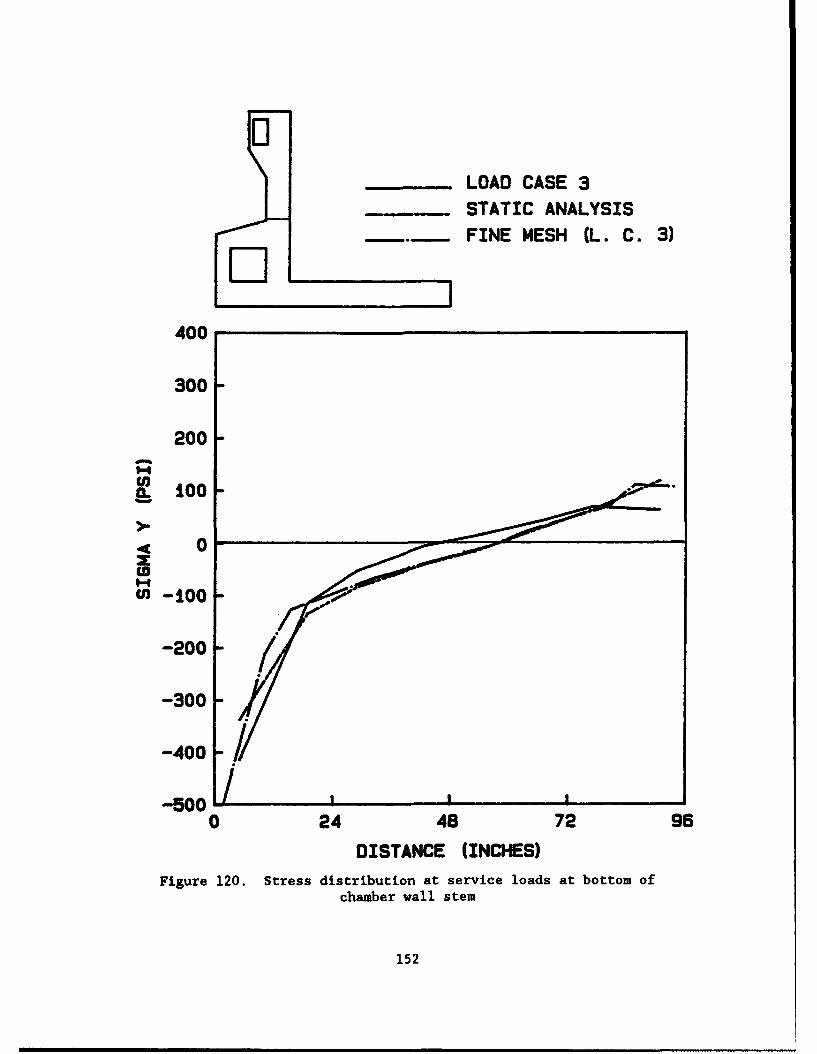
LOAD CASE 3
STATIC ANALYSISFINE MESH (L. C. 3)
I
400
300
200
I-I
0
U) -10 -
-200
-300
-400
-500-/1,
0 24 48 72 96
DISTANCE (INCHES)
Figure 120. Stress distribution at service loads at bottom ofchamber wall stem
152
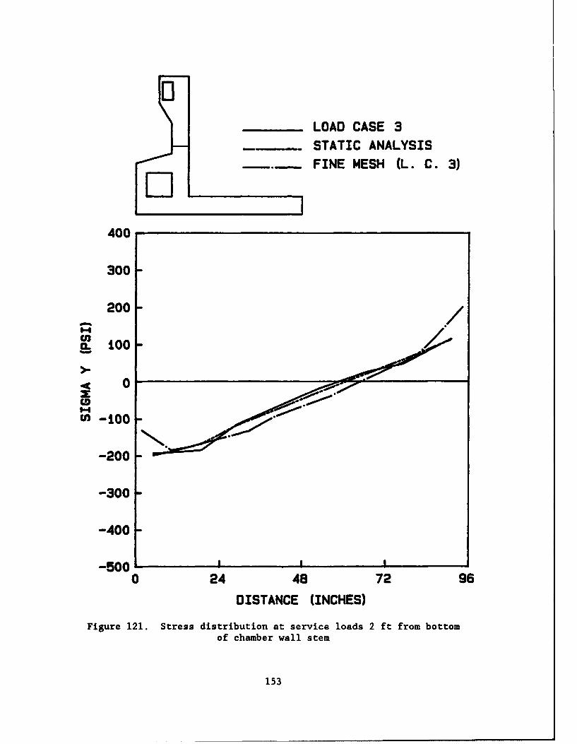
.,, LOAD CASE 3
STATIC ANALYSIS
FINE MESH (L. C. 3)
400
300
200
W O
0Ca
U) -100
-200
-300
-400
-5000 24 48 72 96
DISTANCE (INCHES)
Figure 121. Stress distribution at service loads 2 ft from bottomof chamber wall stem
153
the dead weight applied as an earthquake load, and the large vertical load
associated with the wall. The increase in stress in both Figures 115 and 116
at 60 in. followed by a decrease is related to the lift interface and the
residual thermal effects.
87. Figure 117 and 118 show the flexural stresses resulting in the lock
wall on both sides of culvert. These stresses are also due primarily to the
hydrostatic force on the chamber wall and the earthquake force. The right
culvert wall could act like a tension strut while the left culvert wall would
act like a compression strut, but, looking at the deflection plot for the
parametric analysis in Figure 122, it can be seen that the curvature of both
walls indicate the stress distributions are correct. A similar deflection is
obtained for the static analysis except that the left side of the lower part
of the structure does not have the displacement to the right which is caused
by shrinkage.
88. Figure 119 shows the stress distribution for a cut through the roof
of the culvert. The tensile stress at the bottom of the culvert roof is due
primarily to the dead weight of the concrete above the culvert.
89. Figures 120 and 121 show the stresses in the stem of the chamber
wall. Again, a flexural situation is a result of the hydrostatic force and
the earthquake force. Figure 121 is included to show that the high stresses
at the corner is a result of stress concentrations.
90. All of the figures show that the analyses produce similar results
especially in the sense that the resulting moments are in the same direction
and of the same relative magnitude. Thus, it is acceptable for a simple
static analysis to be performed when dimensioning the structure, saving the
engineer valuable time in the preliminary design phase. When the structure is
designed for service loads, a thermal analysis should then be performed to
check stresses resulting from the construction process especially resulting
from the heat "buildup." The results of the refined mesh give further con-
fidence in the results obtained from the original mesh.
Pile Forces
91. As was just shown, the engineer can perform a static analysis to
design the structure. It will now be shown that the same conclusion can also
be made for determining the pile forces for designing the pile layout.
154
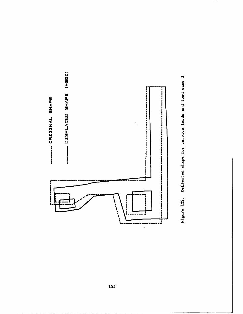
0
CU 0
z 4* aIii a
9 ILo
m H
0. ,a
00
4 -I 4
I'1 1
O 4I
o O
o i:I* CU
oWH J
t II I 0
1C14
I I I C4o
"014U.~~~~~ ........... 4
155
Table 6 shows the results of the spring forces for the static linearly elastic
analysis and the nonlinear, incremental construction analysis including ther-
mal loads. The results for the vertical component are nearly the same espe-
cially under the lock wall where the forces are the greatest. The horizontal
components are greatly different. This is because of the thermal loads which
cause the structure to shrink toward the center line. However, these forces
are not as significant since the H-plies, not battered, are selected to sup-
port the vertical load and checked for adequacy in the horizontal direction.
156
PART VIII: OVERVIEW, INTERPRETATION, AND VERIFICATION OF RESULTS
FOR MONOLITH AL-5
Introduction
92. The significant findings from the results will be further dis-
cussed. In addition, assessments will be made on what these results mean to
the overall structural response of the chamber monolith. Finally, the results
from the finite element program will be verified by checking internal and
external equilibrium.,
Overview. Significance and Interpretation of CalculatedTensile Stress Results
93. The major points of this investigation will now be highlighted.
First, it was found that the upper bound adiabatic curve produced higher tem-
peratures in the structure as would be expected. Next, three stress analyses
were made with creep and shrinkage fixed, and the adiabatic curve set at the
upper and lower bounds and neglected in the third analysis. From this series
of analyses, it was concluded that the upper bound adiabatic curve produced
higher tensile stresses. Consequently, the upper bound adiabatic curve was
used in the remainder of the analyses. In addition, the results of these
analyses also showed that thermal loads produced tensile stresses in locations
where a gravity turn-on analysis showed consistently compressive stresses. As
shown earlier, neglecting thermal loads produces lower stresses. Quite often
the nonthermal analysis predicts compressive stress; whereas, the thermal
analysis predicts tensile stresses. Thus, performing a thermal analysis is
important to locate potential areas for tensile reinforcing.
94. The results from the parametric analysis of creep and shrinkage
indicated that both creep and shrinkage tend to have a softening effect on the
stresses (i.e. creep and shrinkage reduce thermal induced stresses) when the
dominate mode of restraint is internal. Stresses near external restraints
show the opposite to be true, but the difference among the various load cases
for the stresses is not as significant (Figures 83 and 85). A major conclu-
sion is that the design engineer could generally neglect creep and shrinkage
to simplify the analysis without sacrificing any structural integrity.
157
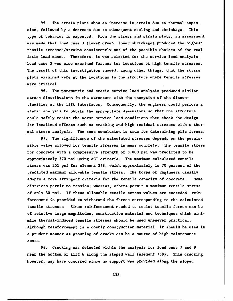
95. The strain plots show an increase in strain due to thermal expan-
sion, followed by a decrease due to subsequent cooling and shrinkage. This
type of behavior is expected. From the stress and strain plots, an assessment
was made that load case 3 (lower creep, lower shrinkage) produced the highest
tensile stresses/strains consistently out of the possible choices of the real-
istic load cases. Therefore, it was selected for the service load analysis.
Load case 3 was also examined further for locations of high tensile stresses.
The result of this investigation showed, among other things, that the stress
plots examined were at the locations in the structure where tensile stresses
were critical.
96. The parametric and static service load analysis produced similar
stress distributions in the structure with the exception of the discon-
tinuities at the lift interfaces. Consequently, the engineer could perform a
static analysis to obtain the appropriate dimensions so that the structure
could safely resist the worst service load conditions then check the design
for localized effects such as cracking and high residual stresses with a ther-
mal stress analysis. The same conclusion is true for determining pile forces.
97. The significance of the calculated stresses depends on the permis-
sible value allowed for tensile stresses in mass concrete. The tensile stress
for concrete with a compressive strength of 3,000 psi was predicted to be
approximately 370 psi using ACI criteria. The maximum calculated tensile
stress was 251 psi for element 378, which approximately is 70 percent of the
predicted maximum allowable tensile stress. The Corps of Engineers usually
adopts a more stringent criteria for the tensile capacity of concrete. Some
districts permit no tension; whereas, others permit a maximum tensile stress
of only 30 psi. If these allowable tensile stress values are exceeded, rein-
forcement is provided to withstand the forces corresponding to the calculated
tensile stresses. Since reinforcement needed to resist tensile forces can be
of relative large magnitudes, construction material and techniques which mini-
mize thermal-induced tensile stresses should be used whenever practical.
Although reinforcement is a costly construction material, it should be used in
a prudent manner as grouting of cracks can be a source of high maintenance
costs.
98. Cracking was detected within the analysis for load case 7 and 9
near the bottom of lift 6 along the sloped wall (element 758). This cracking,
however, may have occurred since no support was provided along the sloped
158
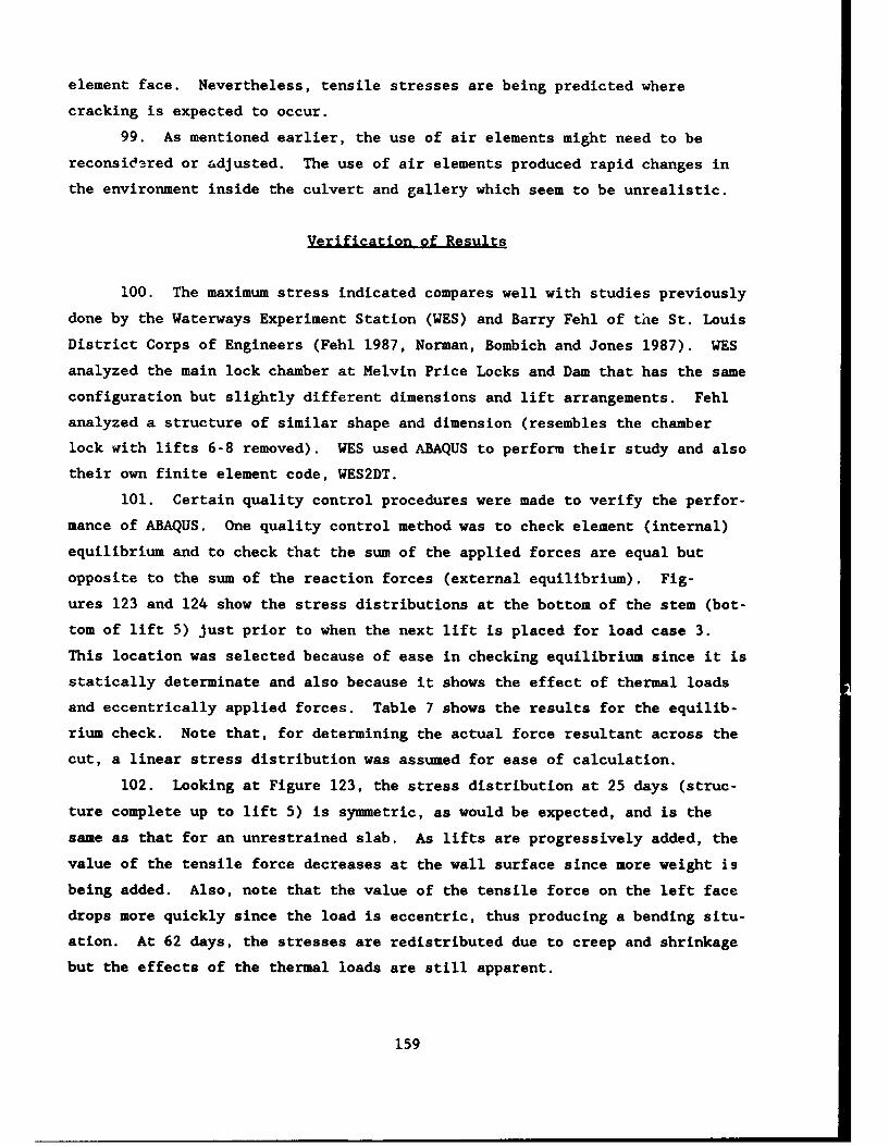
element face. Nevertheless, tensile stresses are being predicted where
cracking is expected to occur.
99. As mentioned earlier, the use of air elements might need to be
reconsidered or adjusted. The use of air elements produced rapid changes in
the environment inside the culvert and gallery which seem to be unrealistic.
Verification of Results
100. The maximum stress indicated compares well with studies previously
done by the Waterways Experiment Station (WES) and Barry Fehl of the St. Louis
District Corps of Engineers (Fehl 1987, Norman, Bombich and Jones 1987). WES
analyzed the main lock chamber at Melvin Price Locks and Dam that has the same
configuration but slightly different dimensions and lift arrangements. Fehl
analyzed a structure of similar shape and dimension (resembles the chamber
lock with lifts 6-8 removed). WES used ABAQUS to perform their study and also
their own finite element code, WES2DT.
101. Certain quality control procedures were made to verify the perfor-
mance of ABAQUS. One quality control method was to check element (internal)
equilibrium and to check that the sum of the applied forces are equal but
opposite to the sum of the reaction forces (external equilibrium). Fig-
ures 123 and 124 show the stress distributions at the bottom of the stem (bot-
tom of lift 5) just prior to when the next lift is placed for load case 3.
This location was selected because of ease in checking equilibrium since it is
statically determinate and also because it shows the effect of thermal loads
and eccentrically applied forces. Table 7 shows the results for the equilib-
rium check. Note that, for determining the actual force resultant across the
cut, a linear stress distribution was assumed for ease of calculation.
102. Looking at Figure 123, the stress distribution at 25 days (struc-
ture complete up to lift 5) is symmetric, as would be expected, and is the
same as that for an unrestrained slab. As lifts are progressively added, the
value of the tensile force decreases at the wall surface since more weight is
being added. Also, note that the value of the tensile force on the left face
drops more quickly since the load is eccentric, thus producing a bending situ-
ation. At 62 days, the stresses are redistributed due to creep and shrinkage
but the effects of the thermal loads are still apparent.
159
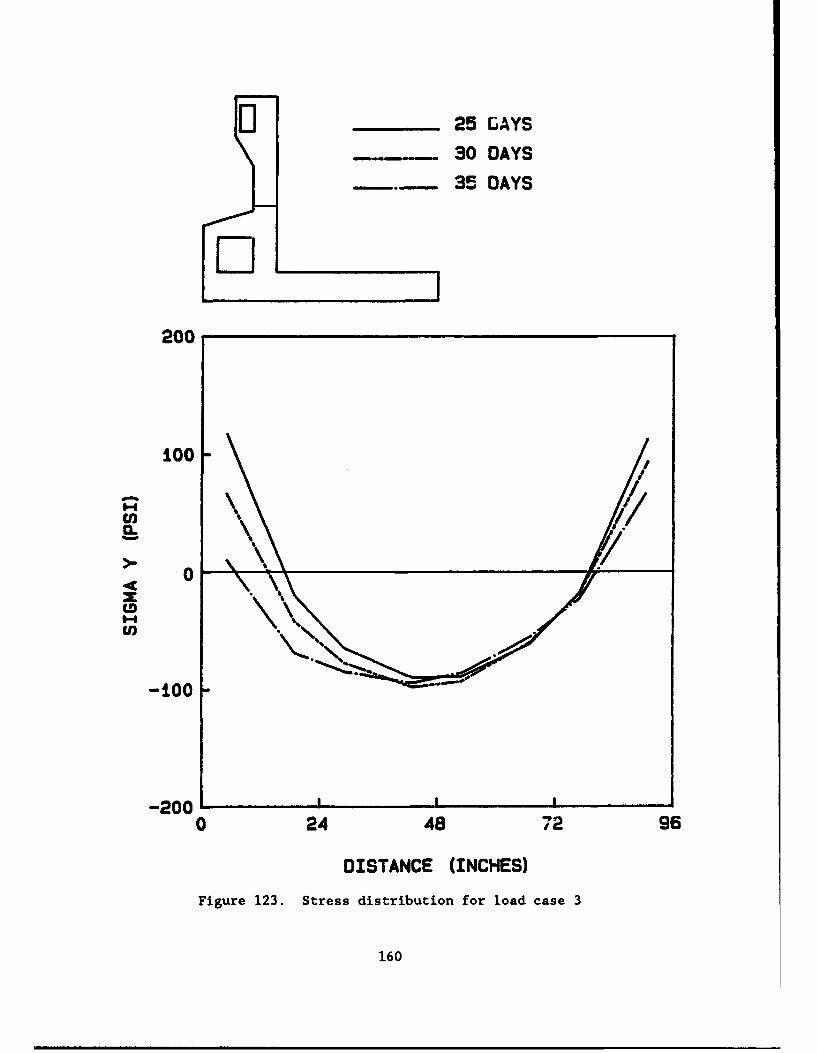
25 LAYS
30 DAYS
35 DAYS
200
100
U)
0
-200
0 24 48 72 96
DISTANCE (INCHES)
Figure 123. Stress distribution for load case 3
160
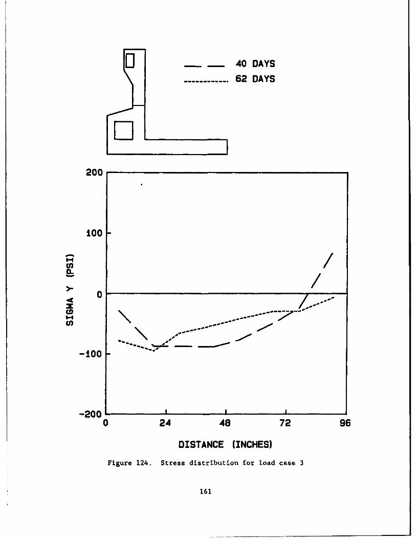
.__-..- 40 DAYS
------------- 62 DAYS
200
100
- /• /
-tO0 -
-2000 24 48 72 96
DISTANCE (INCHES)
Figure 124. Stress distribution for load case 3
161
103. The results in Table 7 show that internal equilibrium is satis-
fied. The largest difference between the internal force and externally
applied force is 8.4 percent at 25 days which is below the acceptable 10 per-
cent. The results at later times are within a few percent.
104. External equilibrium was checked for load case 3 at service loads.
Because the soil elements are iemoved, the calculations are simple as only the
spring forces and the reaction forces at the center line need to be summed and
compared with the sum of the applied forces. The results are shown in Table 8
and indicate external equilibrium is satisfied. Thus, the equilibrium checks
are satisfied and the results from the analysis can be accepted with
confidence.
162
PART IX: MODELING FOR MONOLITH AL-3
Introduction
105. Most of the modelling parameters for AL-5 are identical for AL-3.
The cement type, file coefficients, and finite elements used are the same for
both monoliths. Monolith AL-5 was used to fine tune the procedure and parame-
ters for the analysis of AL-3, but several other studies were performed rela-
tive to AL-3 such as determining the required soil depth and the use of
concrete-soil interface elements.
Finite Element Mesh
106. The finite element mesh and element used in the heat transfer and
stress analyses are shown in Figures 125 and 126. The mesh layout is con-
trolled by (a) the geometry of the structure, (b) the lift heights, and
(c) the maximum size of the elements as dictated by Equation 2. For the con-
crete, the maximum element size was satisfied in both directions. However,
for the soil, the maximum was exceeded in the direction perpendicular to the
heat flow--that is, the horizontal direction. Stretching the element sizes in
the horizontal direction to an aspect ratio of as large as 2:1 was verified,
as mentioned earlier.
Soil DeDth
107. For the heat transfer analysis, including a layer of the soil is
essential. It was thought that, to save computing time, one could replace the
soil with a heat transfer coefficient. However, after the investigation of
several values, it was concluded that a conduction coefficient could not
reflect the effect of the heat exchange between the soil and the concrete.
108. Having decided to include the soil, the soil depth and its initial
temperature were developed. The investigation is based on "how far" below the
surface temperature fluctuations occur and on the effects of changing the
depth of the soil on the temperature rise at the base of the slab.
109. Norman, Bombich, and Jones (1987) stated that the temperature of
the soil is stationary at a depth of 20 ft. However, with the imposed
163
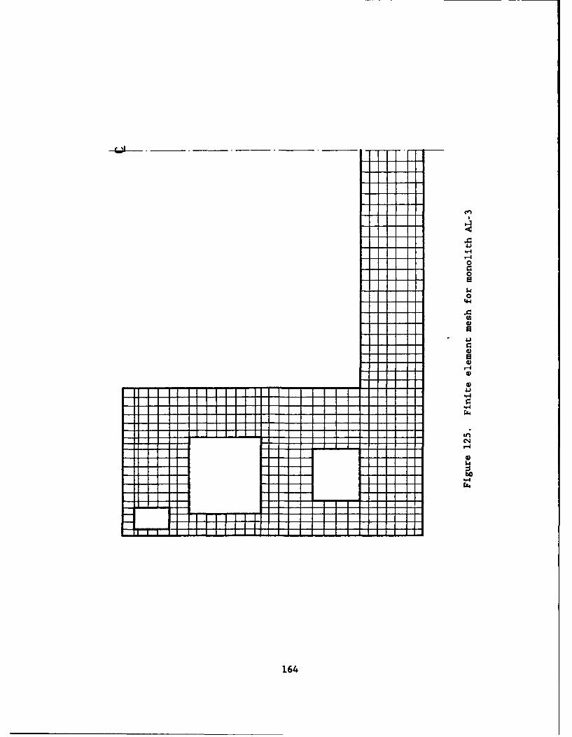
-44
'44
Sli
1644
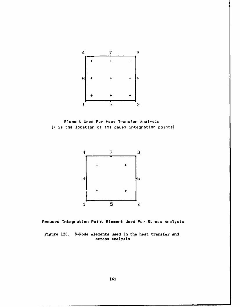
4 7 3
+ + +
8 + + + 6
+ + +
5 2
Element Used For Heat Transfer Analysis
(+ is the location of the gauss integration points)
4 7 3
+ +
8 6
I + +
5 2
Reduced Integration Point Element Used For Stress Analysis
Figure 126. 8-Node elements used in the heat transfer andstress analysis
165
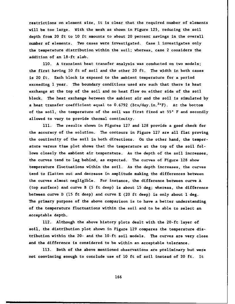
restrictions on element size, it is clear that the required number of elements
will be too large. With the mesh as shown in Figure 125, reducing the soil
depth from 20 ft to 10 ft amounts to about 20 percent savings in the overall
number of elements. Two cases were investigated. Case 1 investigates only
the temperature distribution within the soil; whereas, case 2 considers the
addition of an 18-ft slab.
110. A transient heat transfer analysis was conducted on two models;
the first having 10 ft of soil and the other 20 ft. The w1dth in both cases
is 20 ft. Each block is exposed to the ambient temperature for a period
exceeding 1 year. The boundary conditions used are such that there is heat
exchange at the top of the soil and no heat flow on either side of the soil
block. The heat exchange between the ambient air and the soil is simulated by
a heat transfer coefficient equal to 0.6792 (Btu/day.in. 2 °F). At the bottom
of the soil, the temperature of the soil was first fixed at 550 F and secondly
allowed to vary to provide thermal continuity.
111. The results shown in Figures 127 and 128 provide a good check for
the accuracy of the solution. The contours in Figure 127 are all flat proving
the continuity of the soil in both directions. On the other hand, the temper-
ature versus time plot shows that the temperature at the top of the soil fol-
lows closely the ambient air temperature. As the depth of the soil increases,
the curves tend to lag behind, as expected. The curves of Figure 128 show
temperature fluctuations within the soil. As the depth increases, the curves
tend to flatten out and decrease in amplitude making the differences between
the curves almost negligible. For instance, the difference between curve A
(top surface) and curve B (5 ft deep) is about 15 deg; whereas, the difference
between curve D (15 ft deep) and curve E (20 ft deep) is only about 1 deg.
The primary purpose of the above comparison is to have a better understanding
of the temperature fluctuations within the soil and to be able to select an
acceptable depth.
112. Although the above history plots dealt with the 20-ft layer of
soil, the distribution plot shown in Figure 129 compares the temperature dis-
tribution within the 20- and the 10-ft soil models. The curves are very close
and the difference is considered to be within an acceptable tolerance.
113. Both of the above mentioned observations are preliminary but were
not convincing enough to conclude use of 10 ft of soil instead of 20 ft. It
166
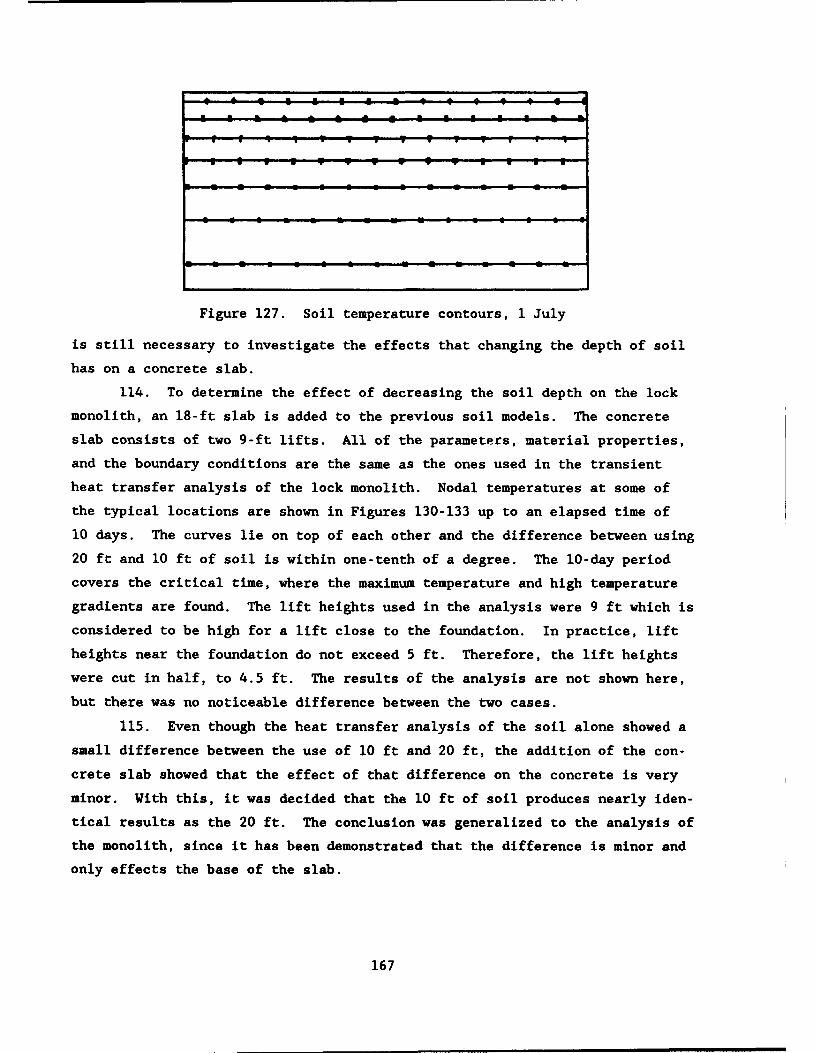
; ; ; ; I & 1 0 - - - - - 4
Figure 127. Soil temperature contours, 1 July
is still necessary to investigate the effects that changing the depth of soil
has on a concrete slab.
114. To determine the effect of decreasing the soil depth on the lock
monolith, an 18-ft slab is added to the previous soil models. The concrete
slab consists of two 9-ft lifts. All of the parameters, material properties,
and the boundary conditions are the same as the ones used in the transient
heat transfer analysis of the lock monolith. Nodal temperatures at some of
the typical locations are shown in Figures 130-133 up to an elapsed time of
10 days. The curves lie on top of each other and the difference between using
20 ft and 10 ft of soil is within one-tenth of a degree. The 10-day period
covers the critical time, where the maximum temperature and high temperature
gradients are found. The lift heights used in the analysis were 9 ft which is
considered to be high for a lift close to the foundation. In practice, lift
heights near the foundation do not exceed 5 ft. Therefore, the lift heights
were cut in half, to 4.5 ft. The results of the analysis are not shown here,
but there was no noticeable difference between the two cases.
115. Even though the heat transfer analysis of the soil alone showed a
small difference between the use of 10 ft and 20 ft, the addition of the con-
crete slab showed that the effect of that difference on the concrete is very
minor. With this, it was decided that the 10 ft of soil produces nearly iden-
tical results as the 20 ft. The conclusion was generalized to the analysis of
the monolith, since it has been demonstrated that the difference is minor and
only effects the base of the slab.
167
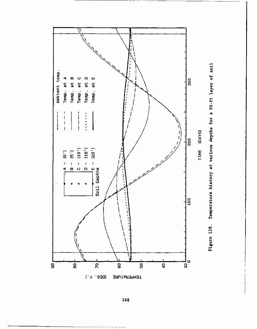
"-4
0
* 144
41 au m au m m 4)~
c:
:11
/ ~4-/C- - -. /P.
a) 01 1
I1 0 0
0. /0 * 0
*rI4
0 0
616
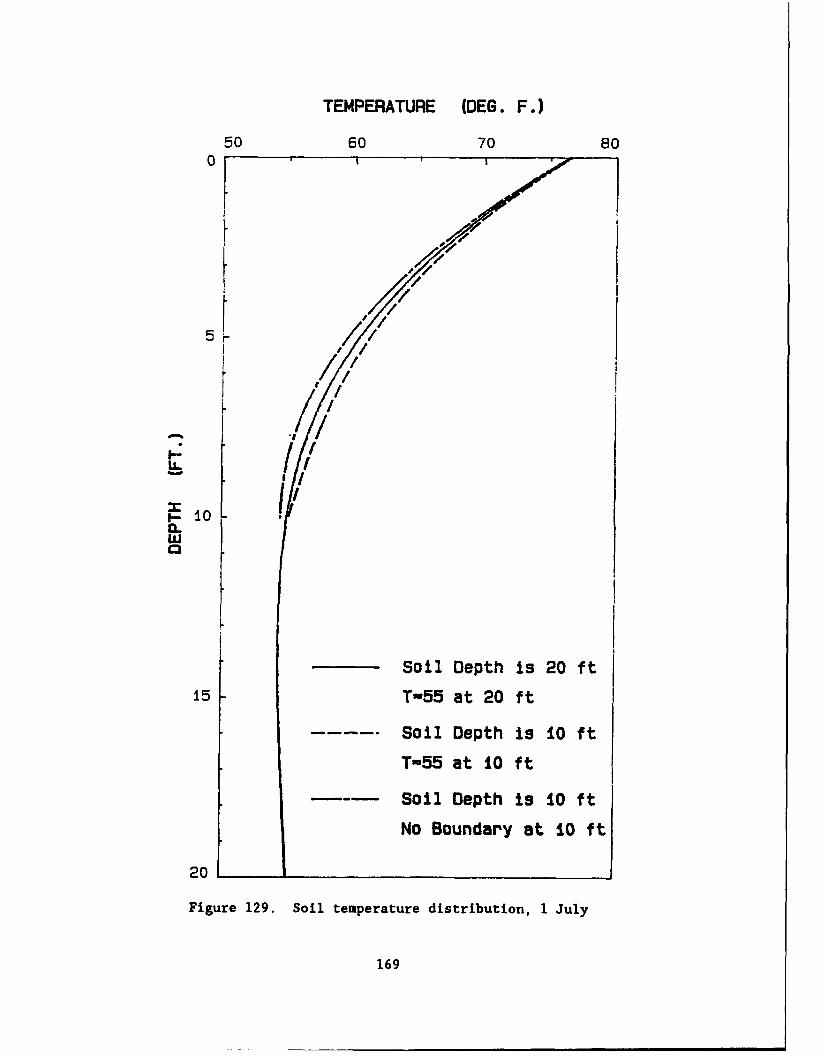
TEMPERATURE (DEG. F.)
50 60 70 800
//
5
/1/
LL 1
10w
Soil Depth is 20 ft
15 T-55 at 20 ft
Soil Depth is t0 ft
T-55 at 10 ft
Soil Depth is 10 ft
No Boundary at 10 ft
20
Figure 129. Soil temperature distribution, 1 July
169
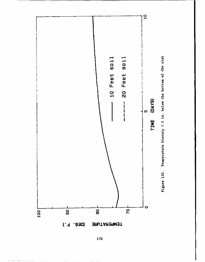
'-44
00 0a) U 0
41
0
4-)
1 > 4Lfl~.0
CA1- '9a 'nVWd
170
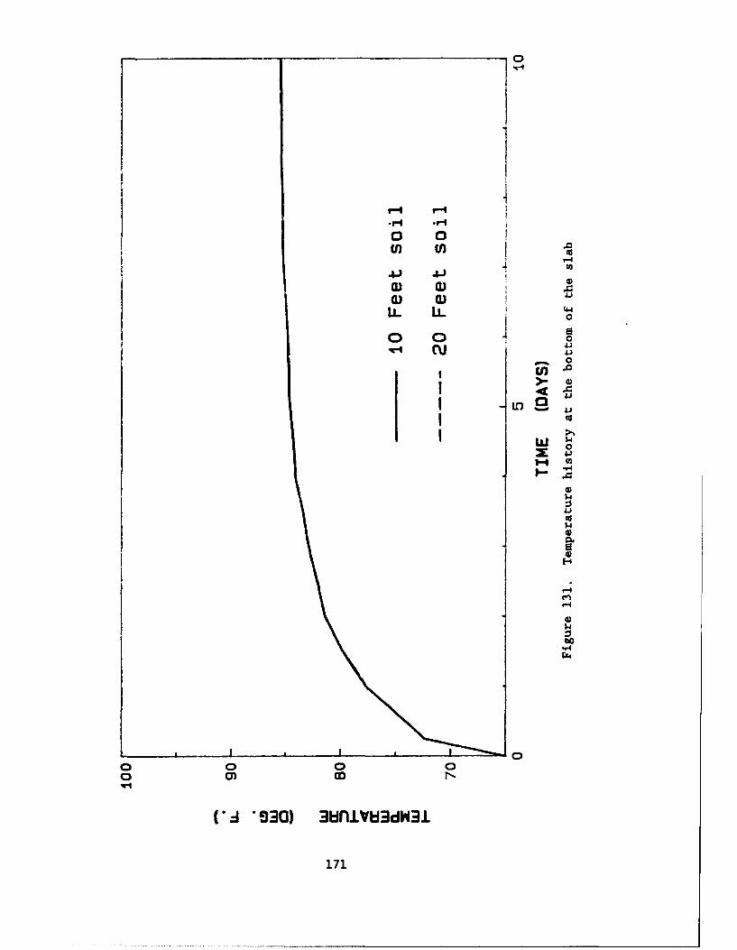
o 0(n U)
.4-I .4.J4-))
a) a) J
Li CUL'44
__0
cn.
'-4
w0
"f4
C..
.4 4
EL-I
on coN
Ad 930) 3bifl1VId3db131
171
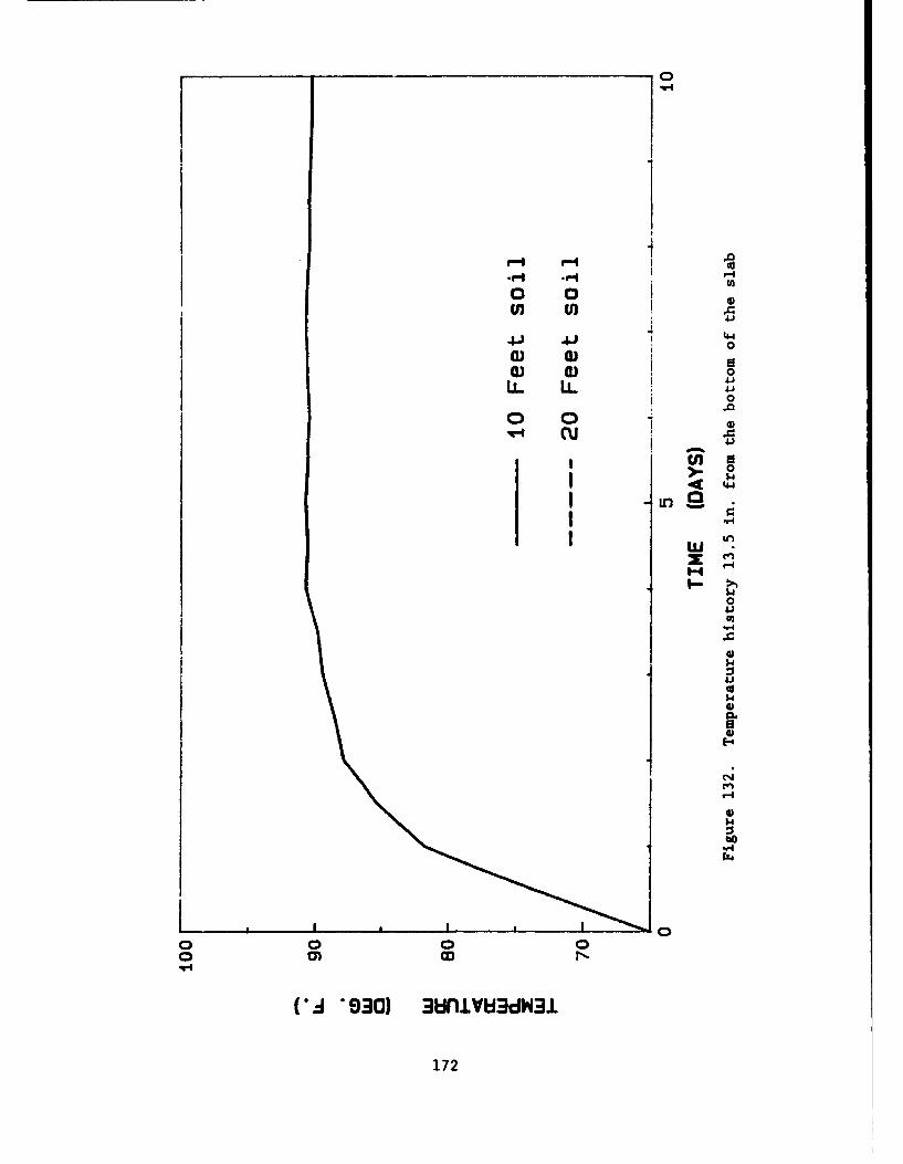
-o4
in o U
* ~4.
a) 03
.00.
o o 0
En.>.0I '.4
1-4
0
34.
E-4
a)en
bo
( 930) 3WifllVbd3dW3l
172
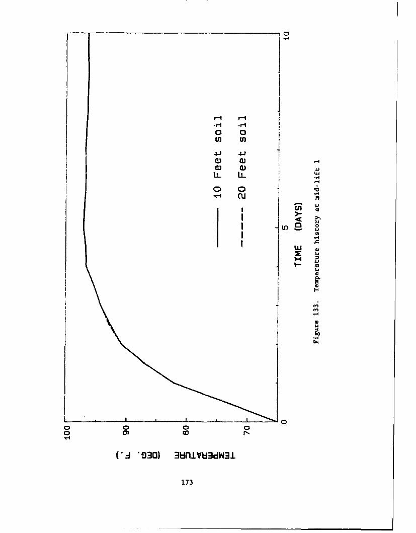
0 0
4ro C)
U) U)
0L 0
4)
1 4
'-4
.4 930) 3unlY1V3dWI43
173
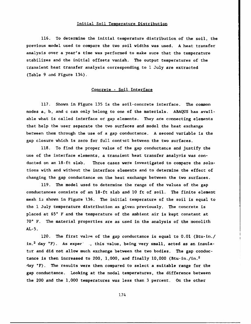
Initial Soil Temperature Distribution
116. To determine the initial temperature distribution of the soil, the
previous model used to compare the two soil widths was used. A heat transfer
analysis over a year's time was performed to make sure that the temperature
stabilizes and the initial offsets vanish. The output temperatures of the
transient heat transfer analysis corresponding to 1 July are extracted
(Table 9 and Figure 134).
Concrete - Soil Interface
117. Shown in Figure 135 is the soil-concrete interface. The common
nodes a, b, and c can only belong to one of the materials. ABAQUS has avail-
able what is called interface or gap elements. They are connecting elements
that help the user separate the two surfaces and model the heat exchange
between them through the use of a gap conductance. A second variable is the
gap closure which is zero for full contact between the two surfaces.
118. To find the proper value of the gap conductance and justify the
use of the interface elements, a transient heat transfer analysis was con-
ducted on an 18-ft slab. Three cases were investigated to compare the solu-
tions with and without the interface elements and to determine the effect of
changing the gap conductance on the heat exchange between the two surfaces.
119. The model used to determine the range of the values of the gap
conductances consists of an 18-ft slab and 10 ft of soil. The finite element
mesh is shown in Figure 136. The initial temperature of the soil is equal to
the 1 July temperature distribution as given previously. The concrete is
placed at 650 F and the temperature of the ambient air is kept constant at
70° F. The material properties are as used in the analysis of the monolith
AL-5.
120. The first valve of the gap conductance is equal to 0.01 (Btu-in./
in. 2 day *F). As expec ., this value, being very small, acted as an insula-
tor and did not allow much exchange between the two bodies. The gap conduc-
tance is then increased to 200, 1,000, and finally 10,000 (Btu-in./in. 2
day °F). The results were then compared to select a suitable range for the
gap conductance. Looking at the nodal temperatures, the difference between
the 200 and the 1,000 temperatures was less than 3 percent. On the other
174
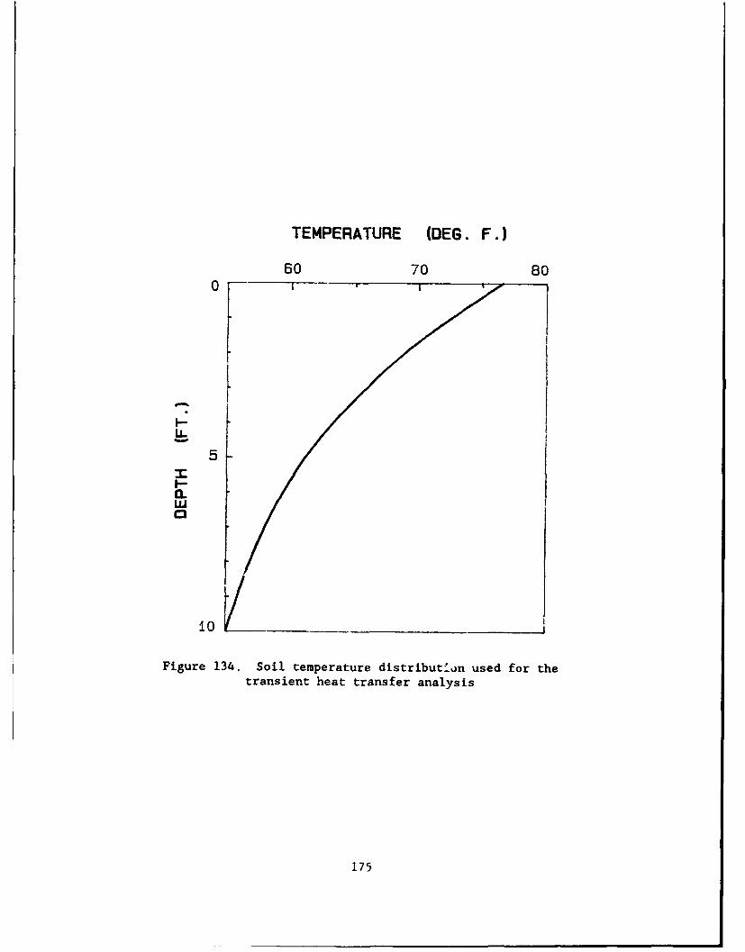
TEMPERATURE (DEG. F.)
60 70 80
"1.
U-
5I-r
0~
10
Figure 134. Soil temperature distribut"_n used for thetransient heat transfer analysis
175
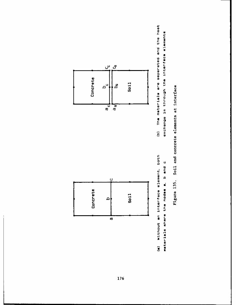
.C a
.0, Cc
'0us0 U
cLy LT2 L a
4J 4
0 -I c
0 m Q
o m c) 4
*m 0 4-)
0 ~ ~w Lf , j
ta I tL -
0 ID
0
0 4.4)
0u
fu
""4
0CO n
10SU En
C L,
L))
£3 a
LI~ wL 0b
(U LU
176-
CU
CONCRETECU
Cu*
- ISOILm.w
15 9 t6 -240" -!
Figure 136. Finite element model used in the interface element study
177
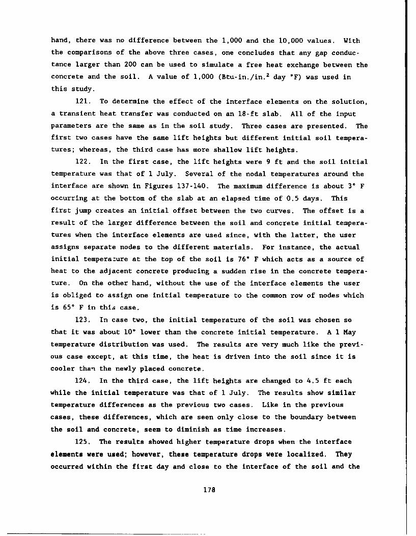
hand, there was no difference between the 1,000 and the 10,000 values. With
the comparisons of the above three cases, one concludes that any gap conduc-
tance larger than 200 can be used to simulate a free heat exchange between the
concrete and the soil. A value of 1,000 (Btu-in./in. 2 day °F) was used in
this study.
121. To determine the effect of the interface elements on the solution,
a transient heat transfer was conducted on an 18-ft slab. All of the input
parameters are the same as in the soil study. Three cases are presented. The
first two cases have the same lift heights but different initial soil tempera-
tures; whereas, the third case has more shallow lift heights.
122. In the first case, the lift heights were 9 ft and the soil initial
temperature was that of 1 July. Several of the nodal temperatures around the
interface are shown in Figures 137-140. The maximum difference is about 3P F
occurring at the bottom of the slab at an elapsed time of 0.5 days. This
first jump creates an initial offset between the two curves. The offset is a
result of the larger difference between the soil and concrete initial tempera-
tures when the interface elements are used since, with the latter, the user
assigns separate nodes to the different materials. For instance, the actual
initial temperature at the top of the soil is 76° F which acts as a source of
heat to the adjacent concrete producing a sudden rise in the concrete tempera-
ture. On the other hand, without the use of the interface elements the user
is obliged to assign one initial temperature to the common row of nodes which
is 650 F in this case.
123. In case two, the initial temperature of the soil was chosen so
that it was about 10* lower than the concrete initial temperature. A 1 May
temperature distribution was used. The results are very much like the previ-
ous case except, at this time, the heat is driven into the soil since it is
cooler than the newly placed concrete.
124. In the third case, the lift heights are changed to 4.5 ft each
while the initial temperature was that of 1 July. The results show similar
temperature differences as the previous two cases. Like in the previous
cases, these differences, which are seen only close to the boundary between
the soil and concrete, seem to diminish as time increases.
125. The results showed higher temperature drops when the interface
elements were used; however, these temperature drops were localized. They
occurred within the first day and close to the interface of the soil and the
178
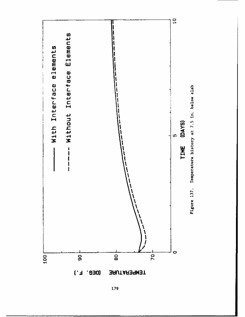
c0
U) )
4-1
a) aCE L
- 10 0)
.C r > .,r
I 04.)w U)n
I '- 4
'.4
0 C)
1794
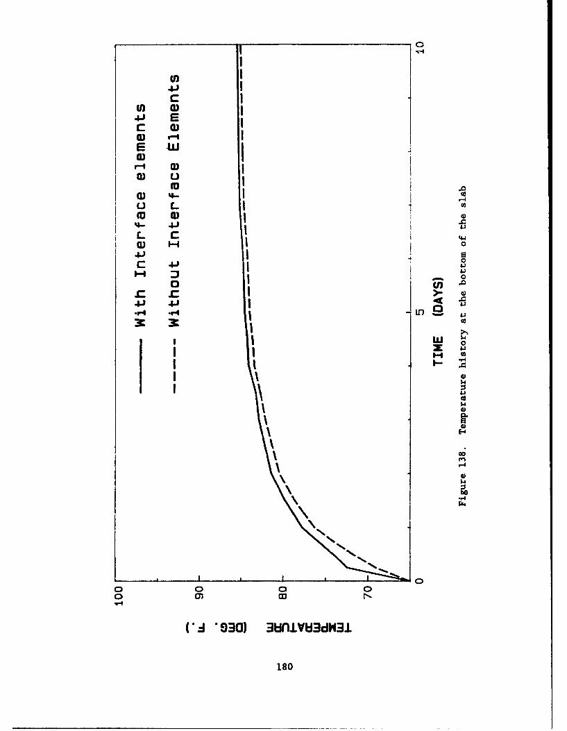
(I)I
(1) a,41 Ec a)Ia) r-
Ir-I a)a) 1)u
L c 4a) 14 0
.1 0
* 0
41 41
.r r 4- i14-
I 0)Ix
I ~4)
34
co'-4
1.4
44
NP
180
U)
4J Ec (DE WUa) *
a) 0
L L 4-
L 4-3-4-
03U)0
41 41 04
LA
It w
4.)
0)
$Z4
0 0~
(*i 0930) 3un.1v83dI43i
181
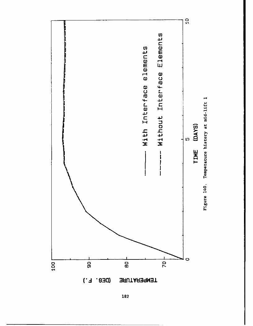
.41
U) a)4-P Ec lE WLa)r-I a)a) u.
CD 4--u L.
L c 4
4-)c 4)"
$4
a~I in2
*,-I *~-i&4)
$4
I*. 000 8VS 3
182
concrete. Thus, for very large massive concrete structures, where one is
interested in locations away from the support or interface or at a later time,
the interface elements are optional and omitting them may save some computing
effort.
126. However, in this study, all the transient heat transfer solutions
use interface elements between the soil and the concrete. Besides giving the
user better control over the input, the interface elements are though to give
a more realistic and better model for the heat exchange between the soil and
the concrete.
Lift Heights
127. For the construction of monolith AL-3, two lift schedules were
provided by the US Army Corps of Engineers, St. Louis District. Configuration
one, composed of 16 lifts, is shown in Figure 141. It is based on an average
lift height of 5 ft. In the slab, the lift heights range from 3 to 4.5 ft;
whereas, in the walls, where the sections are relatively thin, the lift
heights are as high as 6 ft. The second arrangement has only 11 lifts as
shown in Figure 141, which was a means for saving approximately $700,000 in
construction costs (US Army Corps of Engineers, St. Louis District 1988)).
This arrangement allows lift heights as large as 12 ft, eliminating construc-
tion joints and decreasing construction time.
Heat Transfer Analysis
128. For the transient heat transfer analysis conducted for this study,
the time interval between lifts is kept constant at 5 days. The forms were
considered to be removed at 2 days after the lift was placed. These are very
optimistic estimates, but were used since these times should produce the high-
est temperature gradients.
129. Figure 5 shows the mean ambient temperature corresponding to the
site location. The daily fluctuations are ignored to simplify the analysis.
130. Table 10 shows the various surface heat transfer coefficients used
in this study. The coefficients are based on a 0.75-in. plywood form and a
velocity reflecting the air flow through external surfaces and through open
and closed voids like the culvert and the gallery, as discussed earlier.
183
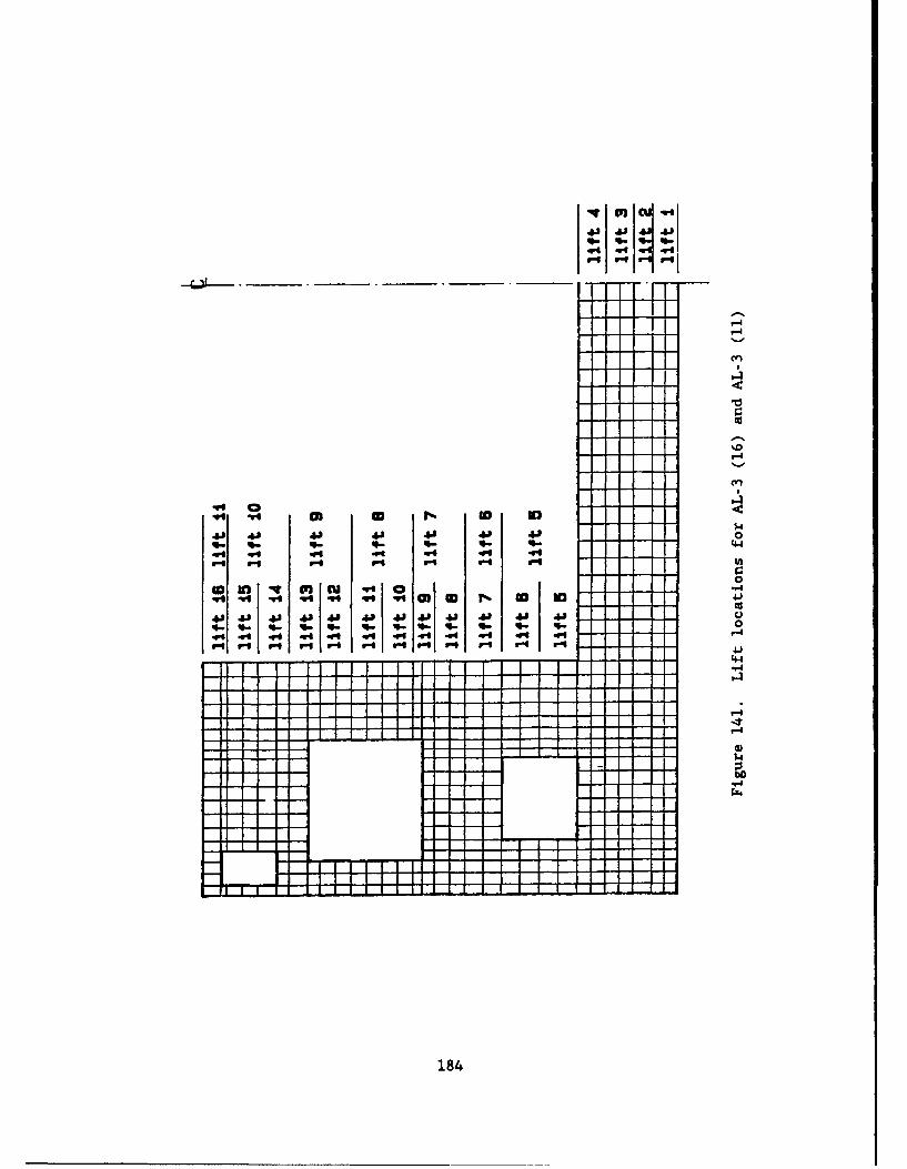
r-4r-4
'U
-4
4'41 ' 4 41 4' 0'4-q ~ q q- q-
0
In. .4 .4. cu -1 a 0 f.. E(U
414 V' W4 4' 4'41 4a 4P 4' 0%. %- %- %- %. %- W. 0
we. . M .4. .4 o .4.. .o -M we f-4-rq V" rq r" V-1 V-4r 0- P rl r4 u-I
-4
-4
441---
184
131. Forms are removed after 2 days in all locations except in roof
structures like the horizontal top surface of the openings. In these areas,
where support is needed, the forms are kept for a period of 7 days through the
use of multipoint constraints, MPC's. It should be noted that, in practice,
the forms used in most of the openings like the culverts and the galleries are
one-piece boxes that are placed at the start of the placement of lifts around
the openings and are not removed until 7 days after the opening is closed.
132. The openings are treated like exterior surfaces until they are
closed. As shown in Table 10, lower heat transfer coefficients are used after
closing because of the low air flow through the openings. Once the lift cov-
ering the opening is placed, the opening is then modelled as either closed,
where the air elements are activated, or open where heat transfer coefficients
are used to define the heat exchange between the concrete and the ambient air.
For the monolith under investigation, the machine room, which is referred to
as the void, is modelled as being closed with air properties assigned to the
enclosed space. On the other hand, the gallery and the culvert are modelled
as open since during construction or in service they are assumed to be open
with air flowing through them.
133. The properties used in all of the analyses are summarized in
Table 11. Lower and upper adiabatic temperature rise curves and heat of
hydration curves for two different types of cement, 53 cal/g and 70 cal/g, are
shown in Figures 8 and 9. In this study, only the upper adiabatic curve is
used for the heat transfer analysis, as discussed in Part IV. The material
properties presented here are as provided by the Waterways Experiment Station
(Norman, Bombich, and Jones 1987).
Stress Analysis
134. The stress analysis is dependent upon several of the modelling
parameters related to boundary conditions, soil strength, pile stiffness,
formwork (MPC), and material properties.
135. The stress related boundary conditions are of two types: (a) sym-
metry and (b) supports. The symmetry boundary condition is achieved by having
rollers along the plane of symmetry. The rollers are free to move vertically
but restrained in the horizontal direction. The supports, on the other hand,
include the soil, piles, and formwork.
185
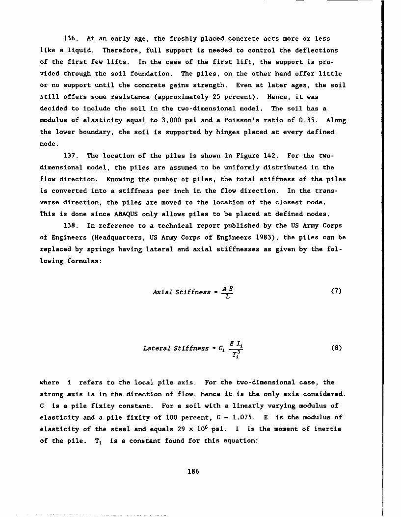
136. At an early age, the freshly placed concrete acts more or less
like a liquid. Therefore, full support is needed to control the deflections
of the first few lifts. In the case of the first lift, the support is pro-
vided through the soil foundation. The piles, on the other hand offer little
or no support until the concrete gains strength. Even at later ages, the soil
still offers some resistance (approximately 25 percent). Hence, it was
decided to include the soil in the two-dimensional model. The soil has a
modulus of elasticity equal to 3,000 psi and a Poisson's ratio of 0.35. Along
the lower boundary, the soil is supported by hinges placed at every defined
node.
137. The location of the piles is shown in Figure 142. For the two-
dimensional model, the piles are assumed to be uniformly distributed in the
flow direction. Knowing the number of piles, the total stiffness of the piles
is converted into a stiffness per inch in the flow direction. In the trans-
verse direction, the piles are moved to the location of the closest node.
This is done since ABAQUS only allows piles to be placed at defined nodes.
138. In reference to a technical report published by the US Army Corps
of Engineers (Headquarters, US Army Corps of Engineers 1983), the piles can be
replaced by springs having lateral and axial stiffnesses as given by the fol-
lowing formulas:
Axial Stiffness = E (7)
Lateral Stiffness = Ci E 1 (8)
where i refers to the local pile axis. For the two-dimensional case, the
strong axis is in the direction of flow, hence it is the only axis considered.
C is a pile fixity constant. For a soil with a linearly varying modulus of
elasticity and a pile fixity of 100 percent, C - 1.075. E is the modulus of
elasticity of the steel and equals 29 x 106 psi. I is the moment of inertia
of the pile. T1 is a constant found for this equation:
186
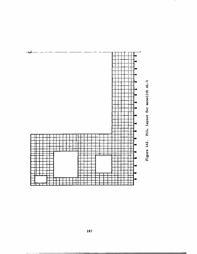
r40
0
0£44
0
-4
-,4
* I I t - -114
187
Ti r n.- (in.) (9)
where nh is the constant of horizontal subgrade reaction or the change in
the soil modulus with depth and was used as nb - 6 (lb/in. 3 ). Given the
above numerical values, the spring axial and lateral stiffnesses were com-
puted, then converted into stiffnesses per inch in the direction of flow as
axial stiffness of 19,750.8 lb/in, and lateral stiffness of 855.7 lb/in.
139. Due to the large size of the problem, assumptions were made to
reduce computing time and simplify the solution. For instance, the forms
offer full support along the surfaces. However, to do a finite element model
of 3/4-in. thick forms or to replace them with elastic -upports was unreason-
able at this time. Instead, it is assumed that, at the age of I day, the
concrete has more or less hardened and is able to support its own weight.
Before that, the weight of the freshly placed concrete is applied as a uniform
pressure to the previous lift. This assumption was found to work well. On
the other hand, for the roofs of the openings where supports are needed for
longer periods, the forms are replaced by MPC, as discussed earlier. The idea
is to have all the nodes at the roof displace following a prescribed function.
In this study, a linear function between the two end nodes of the opening roof
is imposed until 7 days after the placement of the lift closing the opening.
Material Properties
140. Conducting the proper testing to determine the properties of the
materials used is critical for defining the model of a massive concrete struc-
ture where creep, shrinkage, and aging modulus are to be considered. All of
the material properties used in this study were as provided by the Waterways
Experiment Station through the subroutine UMAT (Norman, Bombich, and Jones
1987; Anatech, Inc. 1987) and were discussed in Part III.
188
PART X: RESULTS FROM THE HEAT TRANSFER ANALYSIS FOR MONOLITH AL-3
Introduction
141. The temperature results are presented in forms of temperature
history plots and temperature distribution plots. The figures will show the
temperature variations and their relation to the monolith geometry and model-
ling techniques. Also, a comparison between the 16-lift and the 11-lift mono-
liths show the effects of increasing lift heights. The locations considered
are outside edge, nodes, nodes around the openings, and nodes that are either
at the top or the middle of the lifts shown in Figure 143. These locations
were chosen based on the results from AL-5. They provide an overall view of
typical temperature effects and distributions throughout the monolith AL-3.
General Trends
142. In general, the history plots for the 16-lift model show a sudden
temperature rise at early times, which is most severe for the embedded nodes.
This initial temperature rise does not last longer than 2-3 days. For the
edge nodes, the rise ranges from about 5° F to 100 F above the ambient air
temperatures. Nodes within thick sections and embedded within the lift pro-
duce a temperature rise as high as 30* F. Nodes at the top of the lift expe-
rience two temperature rises. The first is an initial rise that is 3 to
4 degrees higher than the ambient temperature, the second rise is due to the
heat generated from the new lift placed directly above the node. The rise is
as high as 20 degrees in several of the cases.
143. For the nodes along the edges, there is a sudden temperature drop
following the removal of the forms. This is due to the insulating effect of
the 3/4-in.-thick forms. Once the forms are removed, the hot concrete is
exposed to relatively cooler temperatures and hence the temperature drops to
the ambient temperature (see Figures 144-146). The second small temperature
rise shown in Figures 147 and 148 is due to the heat generated from the newly
placed lift. The temperature plot shown in Figure 149 is for a node on the
floor of the chamber. This resulted in a very small temperature increase
above the ambient temperature and a smooth transition instead of a sudden
drop.
189
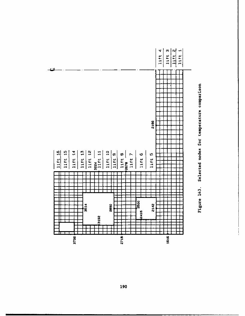
'q m Cu-t
V. 4.1 4.1 4.1
.4 .4- .4-4 4-4
-4 i-1 1-4 r-4
0
0
41.
1.4
04.1
10~~~ InII ' l-.41 1 1 1 1 1 4-0 4J 4-IJ 41Q 41 41
-f . P4 -4 (V. W, 4 m -1 v.4
W- v-I *m .4 -I0
m cu 41':~uijur-4
v-I
I t 4)
mc CU 4C
a' -- -
as In
1'1 Cu w
190
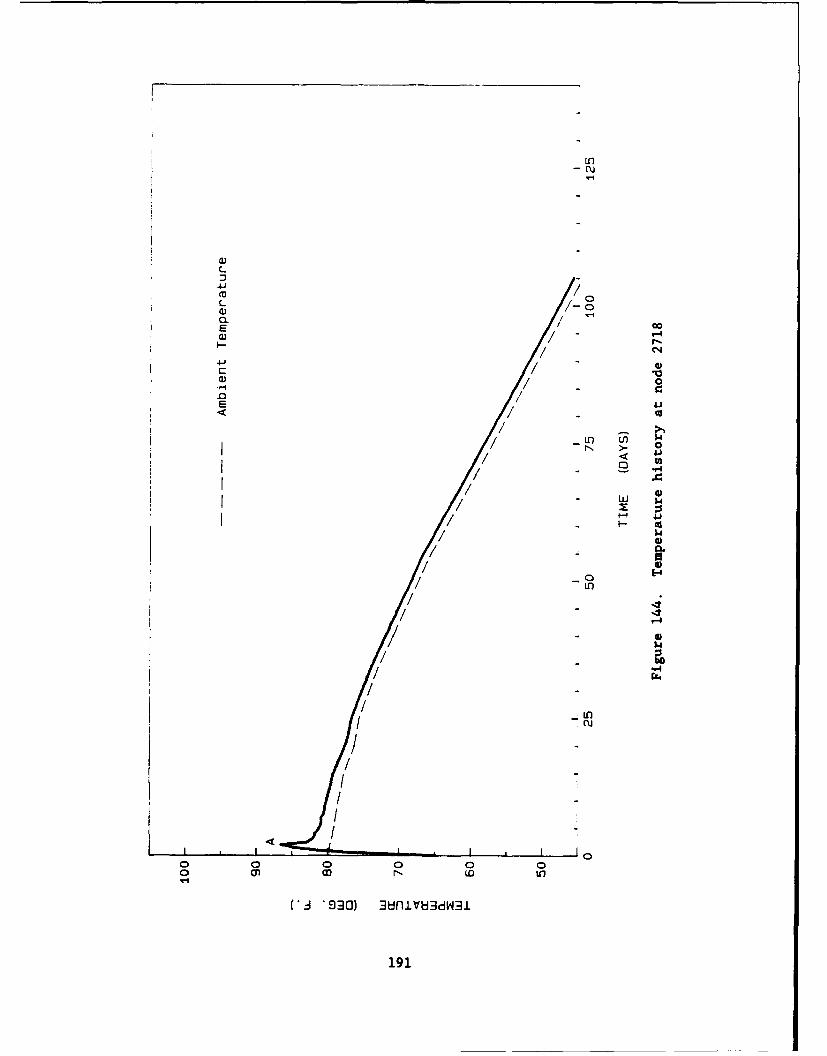
In
4 -J
L7-
/ Cl
c /o
c /0E/
4:5
E /-00
010
CA 3nlV8dW]/
1912
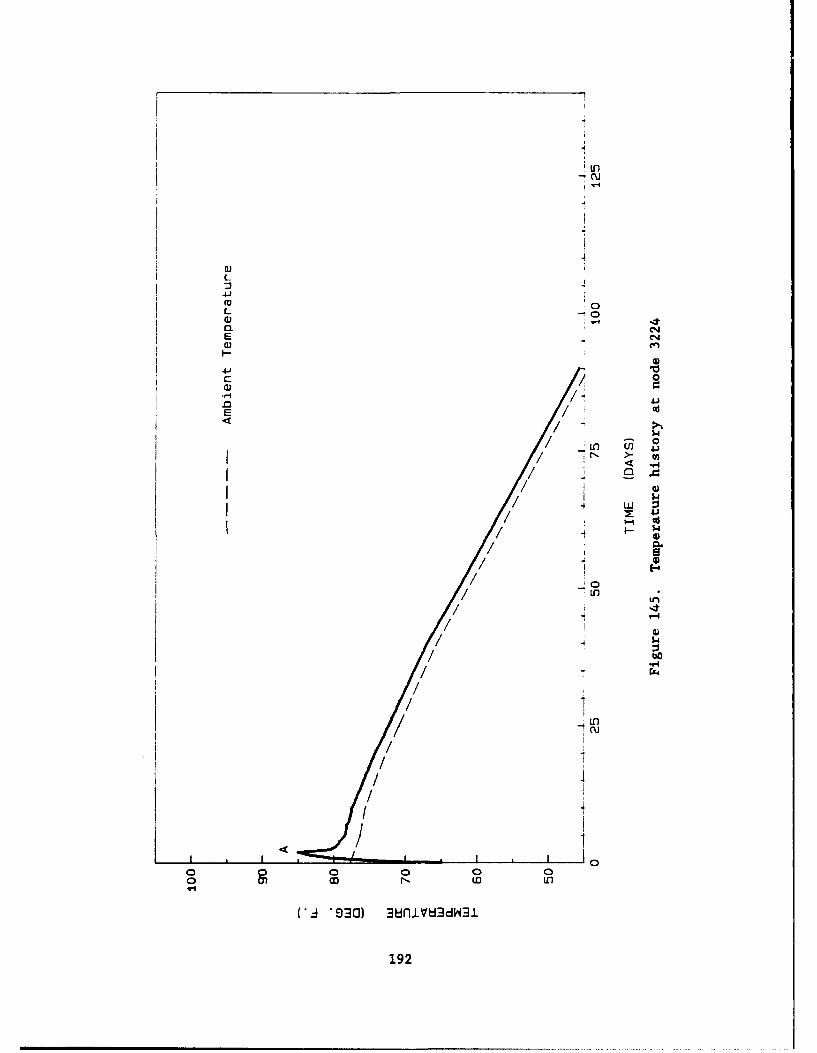
.4
CU)
L -
~ 4)
0.0
E C
I>-
m:. 4-I.0d4$
4 ~14/ -WI
I / 'r,. >-/ I
I /n m (
wlI
CA '00) 3iniV3dW)
192I
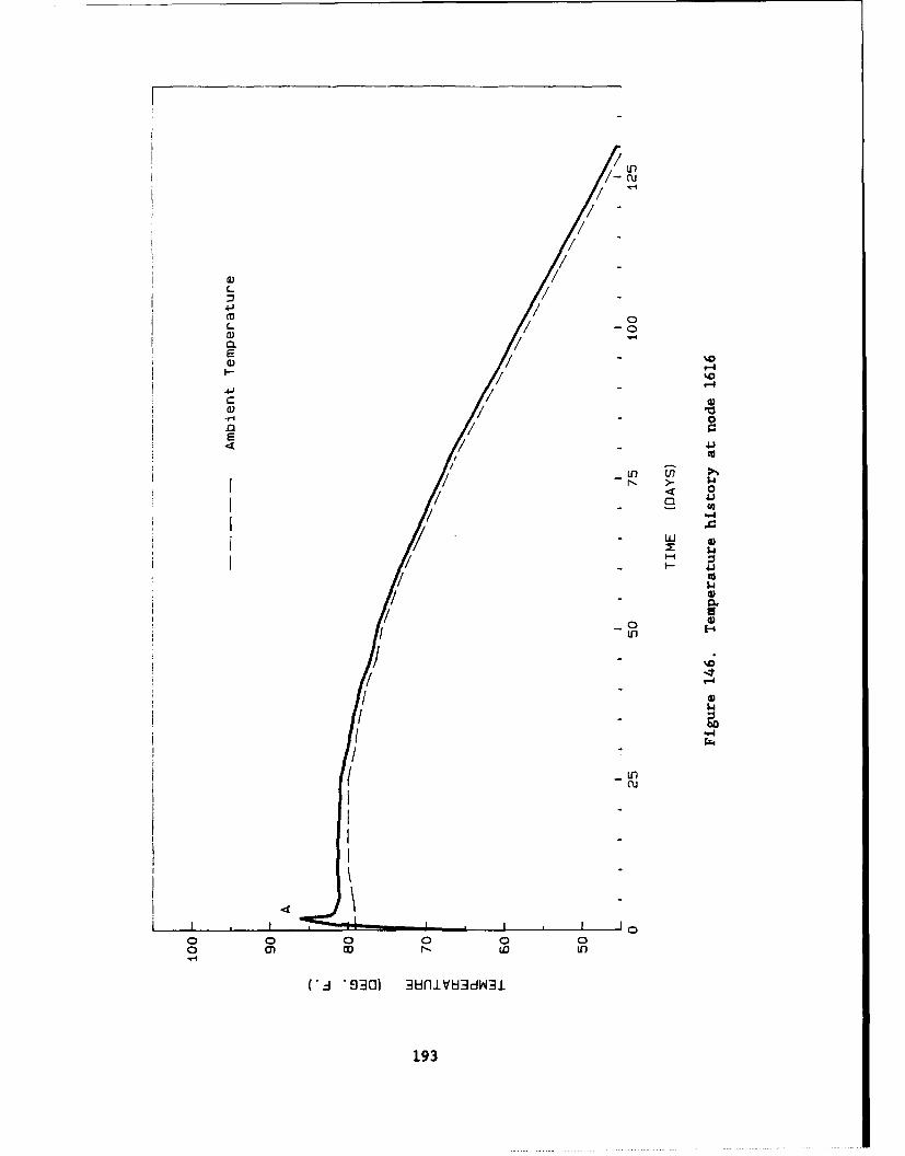
/ -0
I-/41J
/ 0
I->- '-4'
0
/ ~4-/ LUJ
/ 00
0 C) 0C) 0/0~~ wY O L
030) 8niV8dW3I
193-
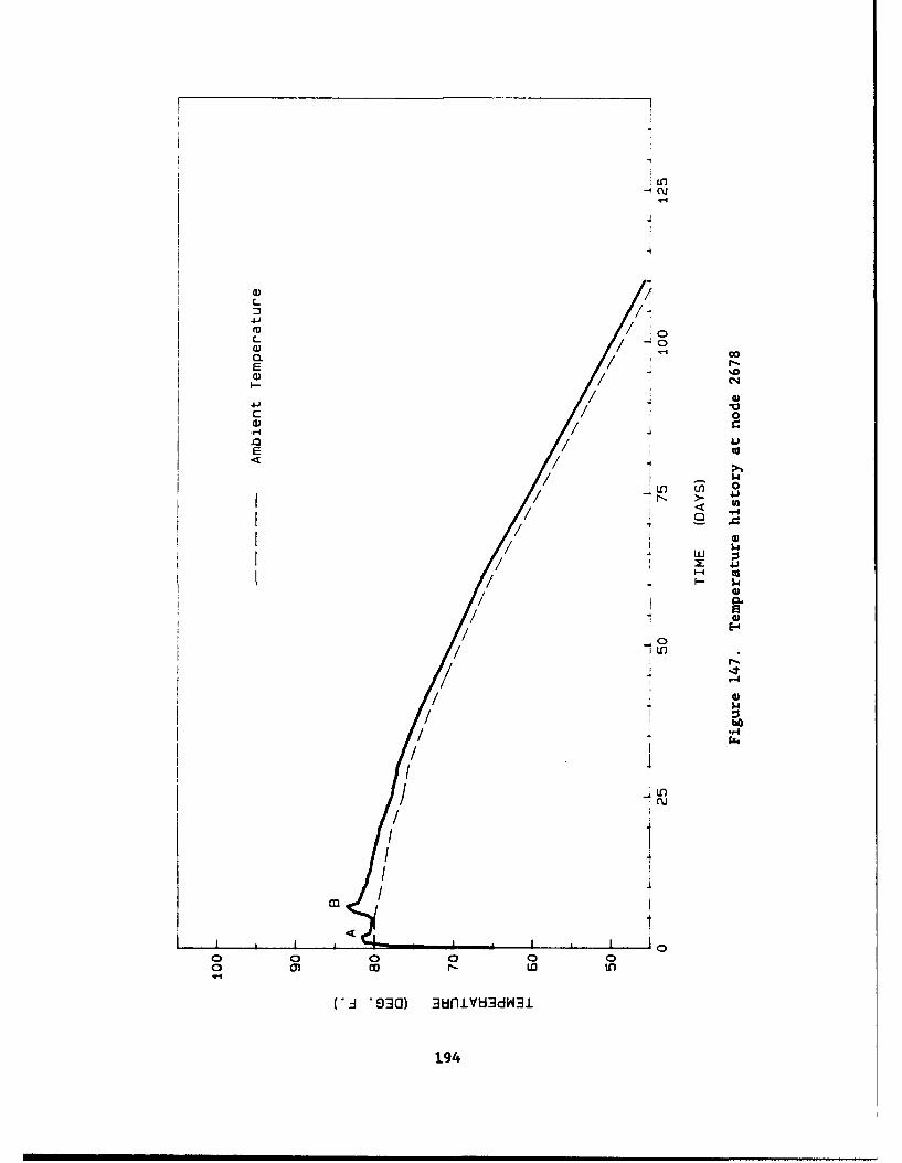
-(\j
a)4
L4
:3 -
a. /a c
/ 1-2 0U
U)L U 0
/ 4 1
-1 tI
0 0/ a)-LDi
/'z '90 ui8dI
194J
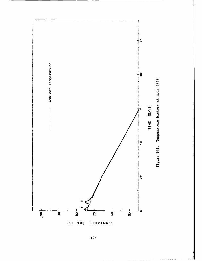
'U,
-c-
L
E -VI
nc
4J JU)c -0
0
0
2
r-4
"54
rz4
Cu
o0 0 0 00oY ci (0 In)
195
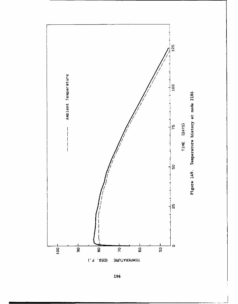
11
/D I
E / 4
c 100J / 0
/ 41
0/ -v .IJ02/r
/ I U4
j /F-4 / 1 @1
'-4
I *1I ~"4
I . O
CA O 38nliVH3dW31
196
144. Several of the curves representing temperature history plots
around the openings are presented to show the difference between the two
modelling techniques which are: (a) activating the air elements to represent
a closed void with no air flow and (b) using reduced heat transfer coeffi-
cients to simulate the heat exchange between the open void and the ambient
air. The difference between the two models is significant. Activating the
air elements creates a connection between the four sides of the opening,
allowing heat to flow freely from one side to the other.
145. An investigation of the temperature regime around the void and the
culvert was conducted. As expected, the use of the reduced heat transfer
coefficients resulted, in a small increase in the temperatures of the surround-
ing concrete. This increase labeled by point C is shown in Figures 150-152.
On the other hand, around the void, where air elements are activated, a jump
in temperatures of 15* F is seen. This is shown in Figures 153-154 at points
labeled D.
146. Figure 155 shows locations where different distribution plots were
made. A temperature distribution plot representing temperature at 5 days
after the placement of lift 9, just before the void is closed, and 15 days
after the void is closed is shown in Figure 156. The first two plots are
similar in shape but the second is lower since heat is lost during the 15-day
period. Figure 157 shows two curves. The dashed curve corresponds to a time
just before the closing of the void, and the solid curve corresponds to a time
15 days after closing the void. For each section on either side of the void,
the temperature distribution has a parabolic shape with the temperature being
low at the sides and increasing as the center of the section is approached,
similar to an unrestrained slab. On the other hand, the second curve, which
corresponds to 15 days after the void has been closed, shows higher tempera-
tures corresponding to the edges of the void. The same curve is plotted in
Figure 158 where the void is eliminated and the two edges are connected. The
curve has a parabolic shape showing that the two sections act more like a
single member with the combined dimensions once the void is closed.
147. Another way of interpreting the temperature results and checking
the heat transfer solution is to look at the temperature distribution plots
along sections as shown in Figure 155. Two sections are presented here. The
first is "cut through" the bed of the chamber, the second is through the mem-
ber between the culvert and the void. The plots are shown at 1/2 day and
197
LO
(D'
L/
E CIA011
031
.1 03
/- 0< 4)
/ ~4.
4 Ir4
/ 003
191
LL
L
40
L- -0
.4J
0)0
-41
>-0< 1C3
"4
U, 4x $4
I:I4
IC
199
(U~
Lc/
cu
/ 100
< Id< 03
/ 14
1.4
/ ~"4I4
I InCu
00 0 0 0 0 0
0n co N tD i
-A '930) flLnV8I3dW3i.
200
L
4.)
(D
.0 0
if) /0
/ r- >-
/ 00
$4
*14
r-4
U) 0
/ '-4
/t/l
0 0 0/0 ED ID ,
201
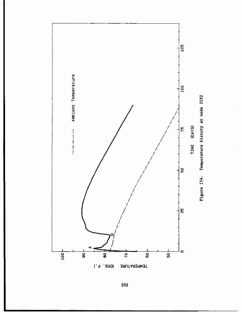
L
0l0
/ 0
/ .44J
/ -'-I
/ ww
/ 0 0 0I n m -E i
/ I- 4dW3
202-
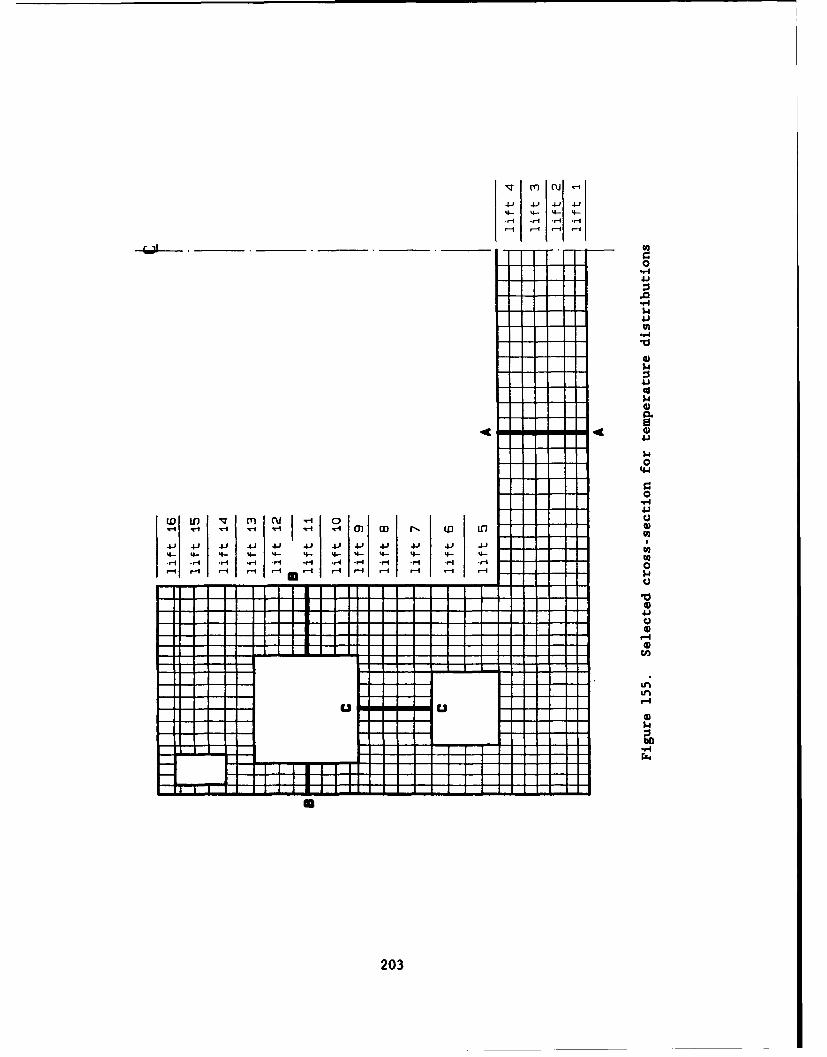
4J) 4J 4-) 4J
4- 4-4- 4
0
"4'$4
"-I
'.4
4.iU'
0
44
0
"4'
-rq 0
41
Ci)4' 4 4' ' 4' 4' ' 4' 4' 4 4' ' U
""4'
203
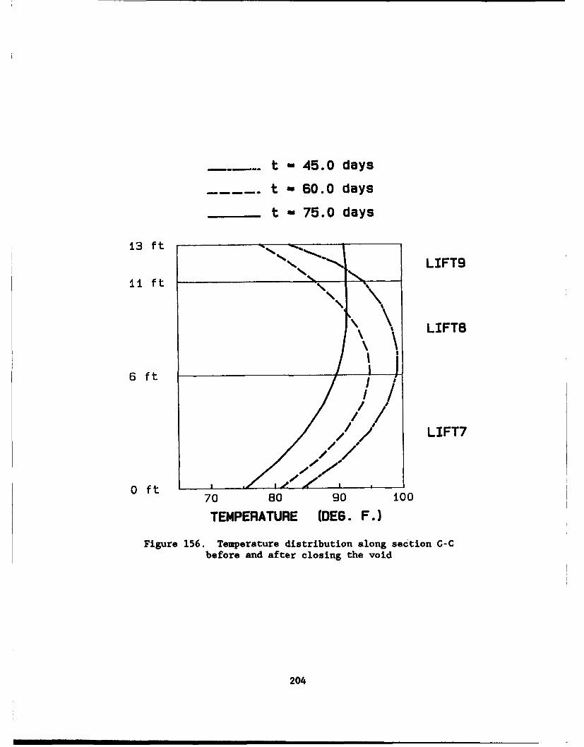
t = 45.0 days
t -60.0 days
t - 75.0 days
13 ft t
"LIFT9
ii ft N
", LIFTS\\ \
6 ft | /
/ // LIFT7,/ //
0 ft70 60 90 100
TEMPERATURE (DE6. F.)
Figure 156. Temperature distribution along section C-Cbefore and after closing the void
204
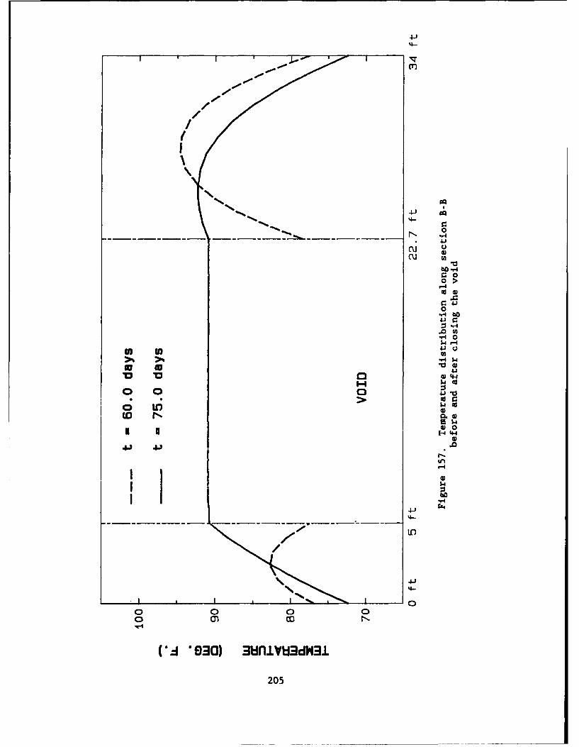
4-I-
oom
-4c,/c
N~ >J
0
.4b0
4J1> CU)
..4 0d
U)
0) 004-
I-Ino o a04
200
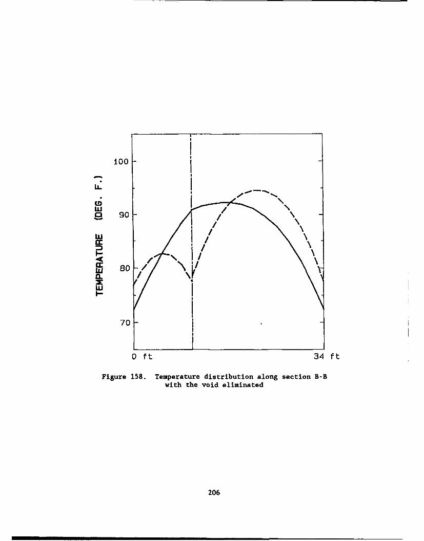
100W!
IL!
2 90
cc
CLu
I--
70 -
0 ft 34 ft
Figure 158. Temperature distribution along section B-Bwith the void eliminated
206
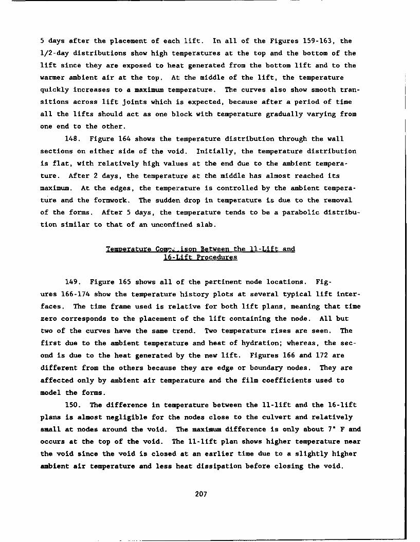
5 days after the placement of each lift. In all of the Figures 159-163, the
1/2-day distributions show high temperatures at the top and the bottom of the
lift since they are exposed to heat generated from the bottom lift and to the
warmer ambient air at the top. At the middle of the lift, the temperature
quickly increases to a maximum temperature. The curves also show smooth tran-
sitions across lift joints which is expected, because after a period of time
all the lifts should act as one block with temperature gradually varying from
one end to the other.
148. Figure 164 shows the temperature distribution through the wall
sections on either side of the void. Initially, the temperature distribution
is flat, with relatively high values at the end due to the ambient tempera-
ture. After 2 days, the temperature at the middle has almost reached its
maximum. At the edges, the temperature is controlled by the ambient tempera-
ture and the formwork. The sudden drop in temperature is due to the removal
of the forms. After 5 days, the temperature tends to be a parabolic distribu-
tion similar to that of an unconfined slab.
Temnerature Comx.e._ison Between the 11-Lift and16-Lift Procedures
149. Figure 165 shows all of the pertinent node locations. Fig-
ures 166-174 show the temperature history plots at several typical lift inter-
faces. The time frame used is relative for both lift plans, meaning that time
zero corresponds to the placement of the lift containing the node. All but
two of the curves have the same trend. Two temperature rises are seen. The
first due to the ambient temperature and heat of hydration; whereas, the sec-
ond is due to the heat generated by the new lift. Figures 166 and 172 are
different from the others because they are edge or boundary nodes. They are
affected only by ambient air temperature and the film coefficients used to
model the forms.
150. The difference in temperature between the 11-lift and the 16-lift
plans is almost negligible for the nodes close to the culvert and relatively
small at nodes around the void. The maximum difference is only about 7* F and
occurs at the top of the void. The 11-lift plan shows higher temperature near
the void since the void is closed at an earlier time due to a slightly higher
ambient air temperature and less heat dissipation before closing the void.
207
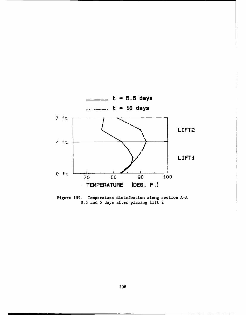
t - 5.5 days
t- i0 days
7 f t
LIFT2
4 ft
LIFTI
0 ft i , I I70 80 90 100
TEMPERATURE (DEG. F.)
Figure 159. Temperature distribution along section A-A0.5 and 5 days after placing lift 2
208
t = 10.5 days
t = 15 days
11.5 ft
LIFT3
7 ft
LIFT2
A ft
LIFTI
O ft70 80 90 i00
TEMPERATURE (DEG. F.)
Figure 160. Temperature distribution along section A-A0.5 and 5 days after placing lift 3
209
_t - 15.5 days
t - 20 days
16 ft
N LIFT4
11.5 ft
I IT
7 ftI1 LIFT2
4 ft
LIFT2
0 ft
70 80 90 100
TEMPERATURE (DEG. F.)
Figure 161. Temperature distribution along section A-A0.5 and 5 days after placing lift 4
210
t = 30.5 days
t w 32 days
t t 35 days
6 ft
/NI LIFT7
II
0 ft -,70 80 90 i00
TEMPERATURE (DES. F.)
Figure 162. Temperature distribution along section C-C0.5, 2, and 5 days after placing lift 7
211
t - 35.5 days
t - 37.0 days
t - 40.0 days
Ii ft N
K LIFT8
6 ft
LIFT7
0 ft --70 80 90 100
TEMPERATURE (DE6. F.)
Figure 163. Temperature distribution along section C-C0.5, 2, and 5 days after placing lift 8
212
4 -J
CT)
- -4
I.elI, Iii w
Cu
%0
4.)
0.
C- -490 3n.kad~
Ifl 0 lii 00213
vm !ru .
r-4
44'44r-4
C0,-4
P-4
bO
-4 o toLUR
411 I& 1 1 .4 1 1 4*. -- . .4 %.- 4-'
.11' -1 - II
-4 41
(D i q c cu0vU
.44
mC
2144
uL-Cu
'-4
'-)10
0
Uni) 0
- F- >- 4.LL L 4
0
-000 (7J -r-LO
2150
U-)
044
0
C.,
/ - 0
9/"/i $
x :3n/ N - 04.)
/c/$
/L - w 1-
/E
0 0 0
CA -930 38iV30~
/ 216
04
-oo
En I
02
x 01
4.)
-.0
IL I n
00-I CDwL
CA~"- '930 _ oV3d
217,
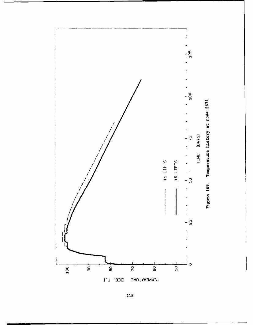
flu
0
-o
- ~ 0
c..
/ JJ
// -n w 0-to
/ -i83W3
/ U) U218
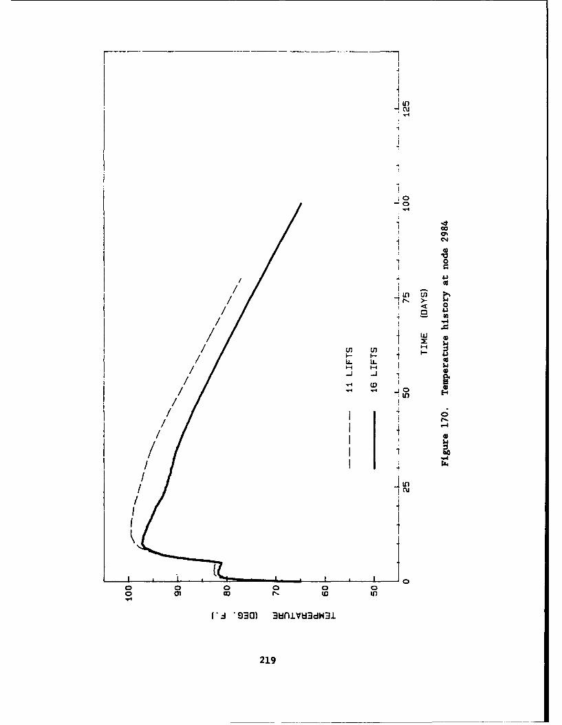
41
,00
-od
.03
L 0%
0
14 0
. 0
I1 1
/wcn w w L
('- '90 4 WV8d3
/ .4 .4 .jO219
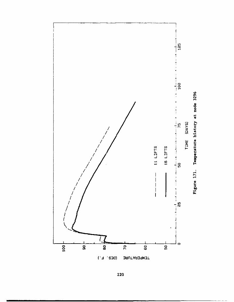
40
0
-oo
~044
m
'U* Lfl $.g
-1 4 -/t 4) '
/n -D weCD
-A '3)/inV1d3
/ j 220
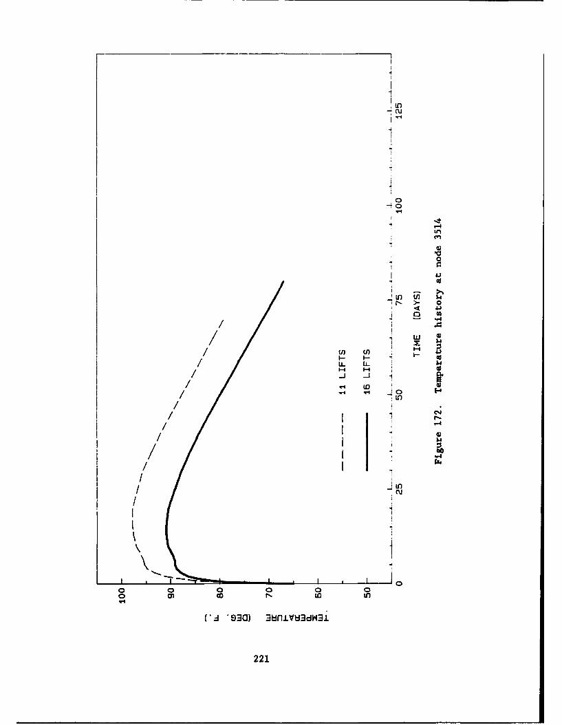
-(U
0.00
r-
I -4"
ui 0
.4$
N- )-
-0 06
/ I )
/C/ U) U)
N L i. In
221
~cu
0
-co
Ln
0
41
>-
En U)/- 10
0;
I- CU
0 00m aD w n
/*: 93) 3di4dd
22
.1
0
-oo
- 04'0
W,
U-- U-
N.) )- r-
030)~ ~ ~ 3u.~f~W.
22
151. Figure 175 shows the appropriate nodes and their locations. Fig-
ures 176-180 show the time history plots (real time) of some of the mid-lift
nodes. Since every proposed lift for the 11-lift schedule is a combination of
two of lifts used in the 16-lift schedule, every figure consists of three
curves. One is for the 11-lift plan labeled B plus the node number and the
other curves which are labeled A plus the node number are for the 16-lift
plan. This was done in order to have a good comparison of embedded nodal
temperatures. The difference is relatively small but it seems to increase for
the upper sections. The maximum difference is only about 5* F to 6° F occur-
ring above the void. Even though this section is relatively thick, the entire
difference in temperature should not be attributed to increasing the lift
height. The ambient temperature, which seen earlier to effect the temperature
rise, is not the same for the corresponding compared sections. For example
the ambient temperature is 79.1° F at the time the void is closed in the
11-lift plan and it is only 75.60 F in the case of the 16-lift plan. The
earlier closing of the void in the 11-lift plan is believed to be the largest
contributor to the difference in temperature between the two lift plans.
224
,q m I u(414J 41 4J
____ ____ ___ FT
4-4
"14
0 Id
r-4
1-4
"14
.4 41 4-1 -W 441
cn m NO L)
r r.1 4 .rI - 4 -H -41 H4 w)~'-4 14 -4 -I 11f rU 4 - ).41
01K~ImH~J.4 IWU
-40
11 H 1 )
w co 0cu m cu L N m4
m 0 l m rl %14Iq o 0 u I in o cm rl w mIq m cu 0 M N Iqm cm m in m m i cu u c cv u-4
4 < 4 m 4 < .4 m
225O
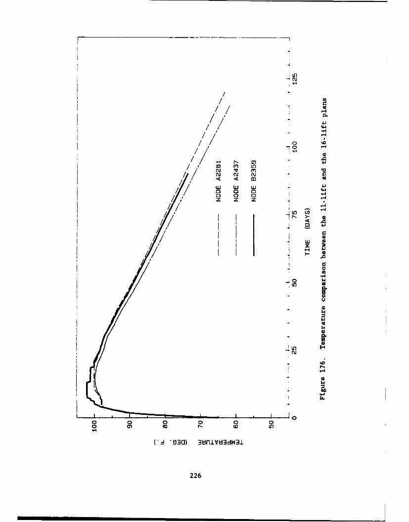
.44
"-4
/ 00
'-4
0)
cu v~ (T
wU w wU 4
'4-iFi
I, I 0/7 I - W
14)
CU
0 00 m ccN (D
930) 3ujvU~4Wi
2264
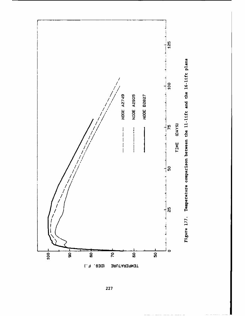
0I g4
4.i
0 41
r4
41
0L
ru w w/ 4 < c
004.
LI 0
I' 1 0
1227
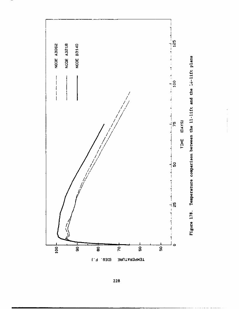
ED CU .4
m m c
wL wi w4o 0 04z z z .
'44.4 '-4-4
'-I
0
"4
/1 1 w 0
0 00~' 04.1r-toL
w7/C4 3un.V834.1
2728
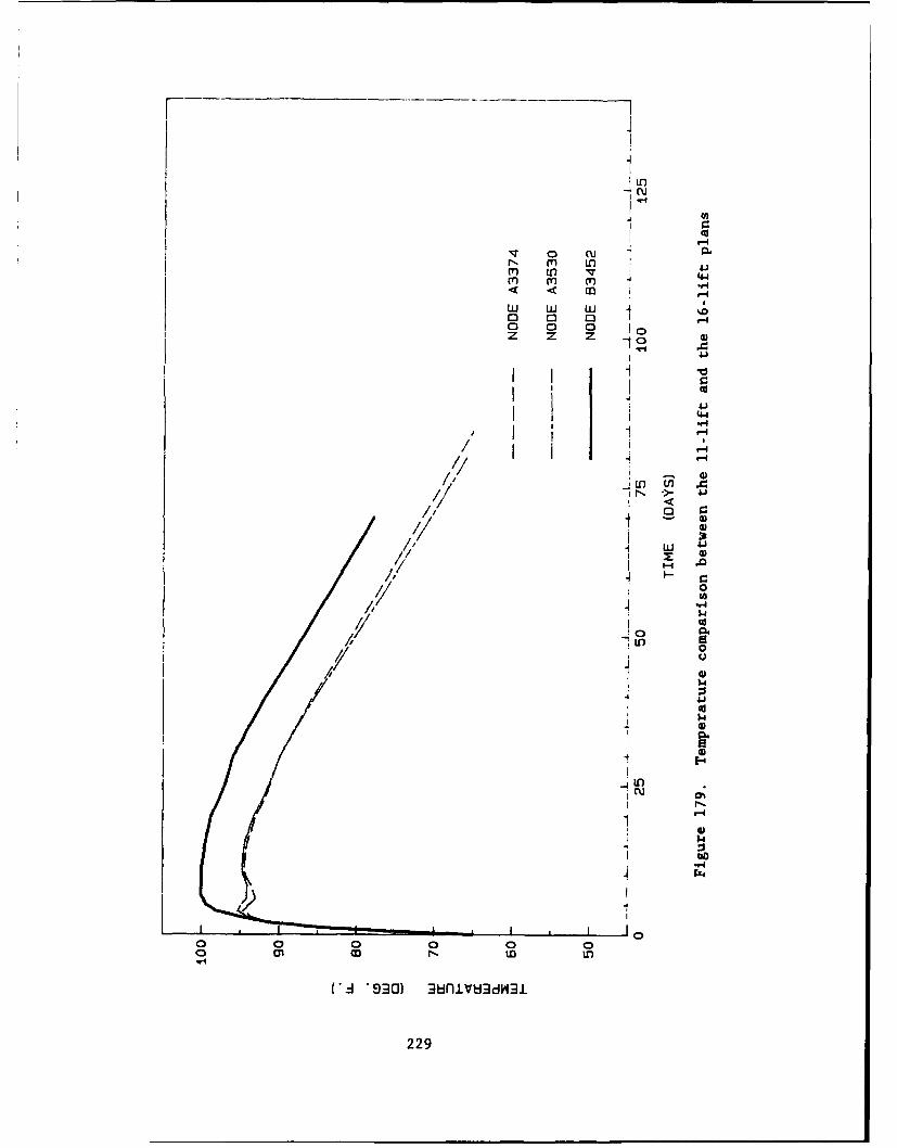
.4
.~ 0 cu a
rn LO n .mv m m 4
4 44
w wL w -Io 0 1 r4o 0 10z z z
4.1
44)
/7 -I, JU U) U.
/ I 0
ii)
$4
14.
E4
- -4
4)
- 4 w4
4$
o0 0 0 0 0on co W In
229
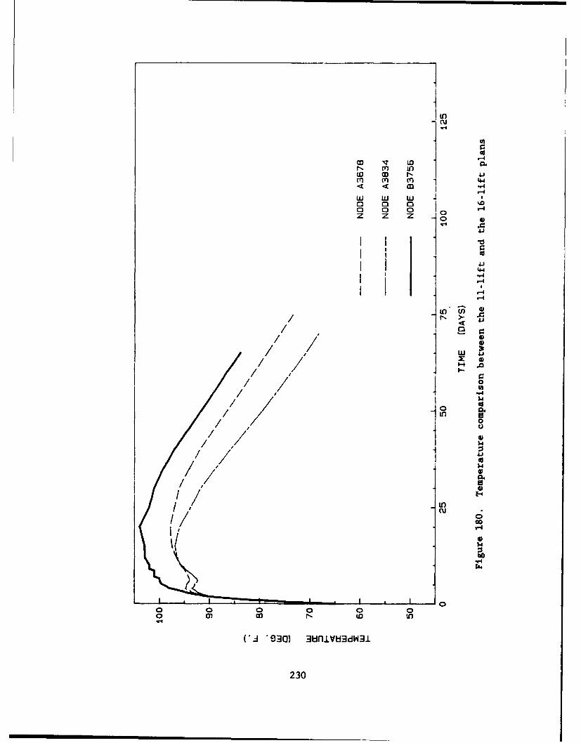
< < m "-
w w w 4
ii 10
/ 1 0// 0
w 43/9
/ / 0 0 0/ .Jc - DL
-/ '90 8iUfd3
/230
PART XI: RESULTS FROM THE STRESS ANALYSIS FOR MONOLITH AL-3
Introduction
152. The results of the stress analysis are presented in forms of his-
tory plots of the horizontal and vertical stresses in forms of stress and
strain distribution plots at some typical sections. The latter are to check
the modelling techniques while the former are mostly used to compare the two
lift schedules.
Incremental Construction
153. As a check to the incremental construction model used, horizontal
stress distributions across the slab were investigated for the 16-lift model.
Even though the stress variations seem to be well behaved within a lift, there
is a discontinuity at the lift interfaces.
154. Two sections are chosen, as shown in Figure 181, to illustrate
this discontinuity. Also, the two extreme load cases of lower creep-lower
shrinkage, LC, LS, UA, and the upper creep-upper shrinkage, UC, US, UA were
used. Section A-A is located about 23 ft to the left of the center line while
section B-B is underneath the culvert 13.6 ft from the left side of the mono-
lith. Both distributions, as shown in Figures 182 and 183, initially have a
parabolic shape which is typical for the newly placed lifts. Both the top and
the bottom of the lift are in tension while the middle is in compression.
This phenomenon is mainly due to the expansion of the slab with increasing
temperature.
155. Temperature rise, as shown in Part X, is not the only parameter
that needs to be considered to interpret the results shown in Figures 182-200.
The slab is supported by piles and by the soil which forms an elastic founda-
tion, coupled with the gravity loads produce bending along with the thermal
effect. This flexure phenomenon is seen clearly in the stress distribution
for section A-A in Figures 184-189. The bottom increases in tension as more
lifts are poured while the top becomes compressive. However, for later times,
as shown in Figure 190, the situation is reversed. Because of the added
weight on either side of the monolith, the slab stresses are reversing with
tension at the top and compression at the bottom. The stress distributions
231
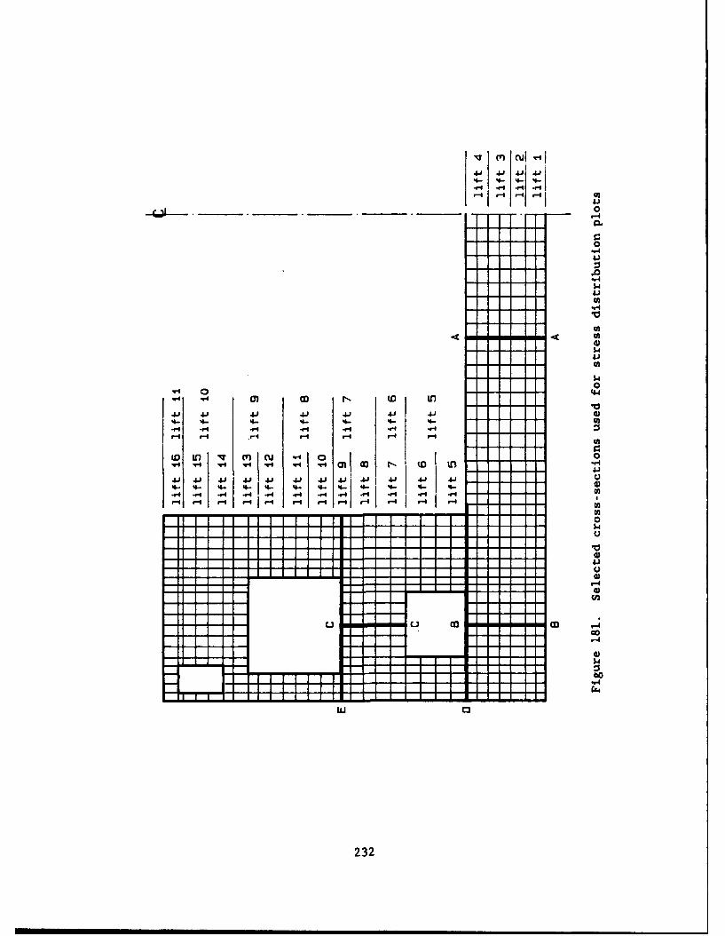
Cfl ('U c
-1-FT T fil
0
"$4
"-4
'.4413U)
"-4
4,cy) (D t- o .4
14
44 0
~4 '.4 1 CD 4
.4.9~ ~~~ .1- .43..1 .3 .3 43
.4- 4- .- .4 .4- .4- 4- U
.44w C3 f4 .4 4 4 4
- 232
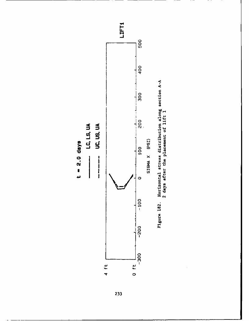
'"4
004
10"4:
KJ 0 404.
0 44 -C
uic 4j0
U) 4 )0o 41U
00
o Icx
'-4
41 4
ror
I
0
-0 cu
0
233
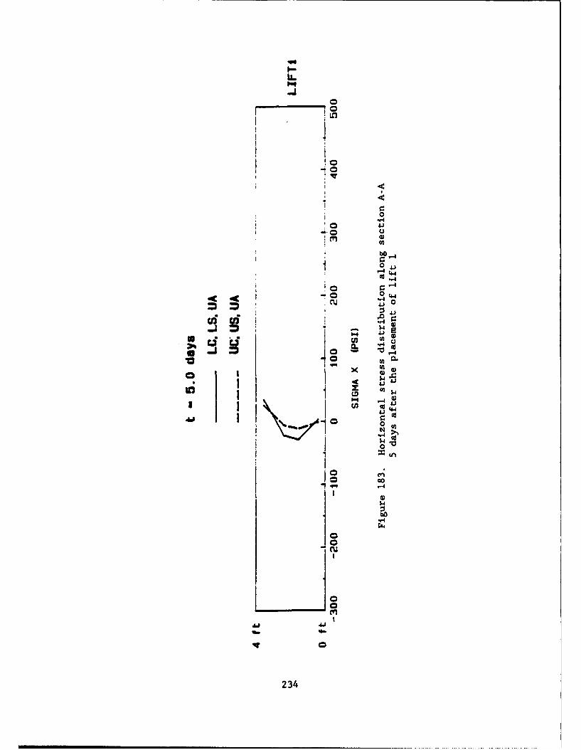
00
'0 44
4*)
jo '0.
0 Mg '2)011
"-4
'-4
00
-Cu
234
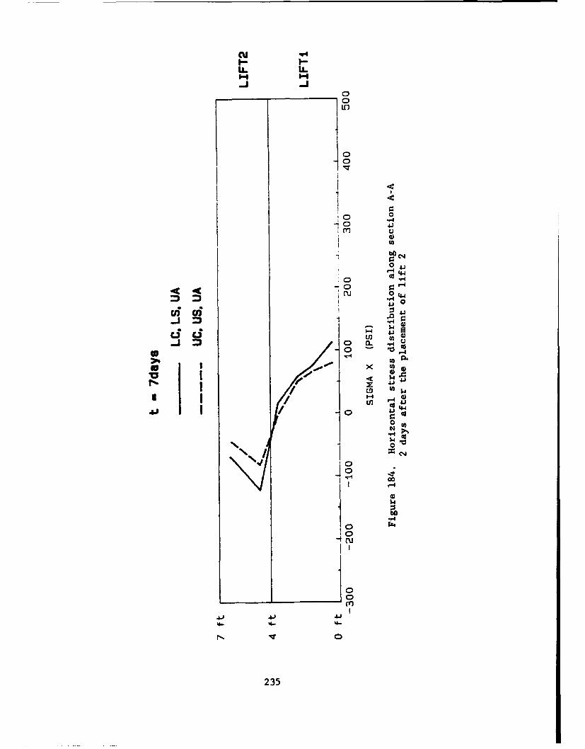
ILn
.0
-00
"-I
-404m4)
r 04
'0
4-,1
I.-.
0
235A
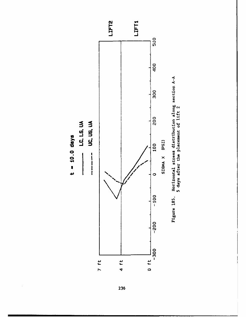
I-
U')
00
ohC)J
0 4
r4J
004
'-44
'-4
00
CD
0 u04.
00____= 0n
J~I
0
236
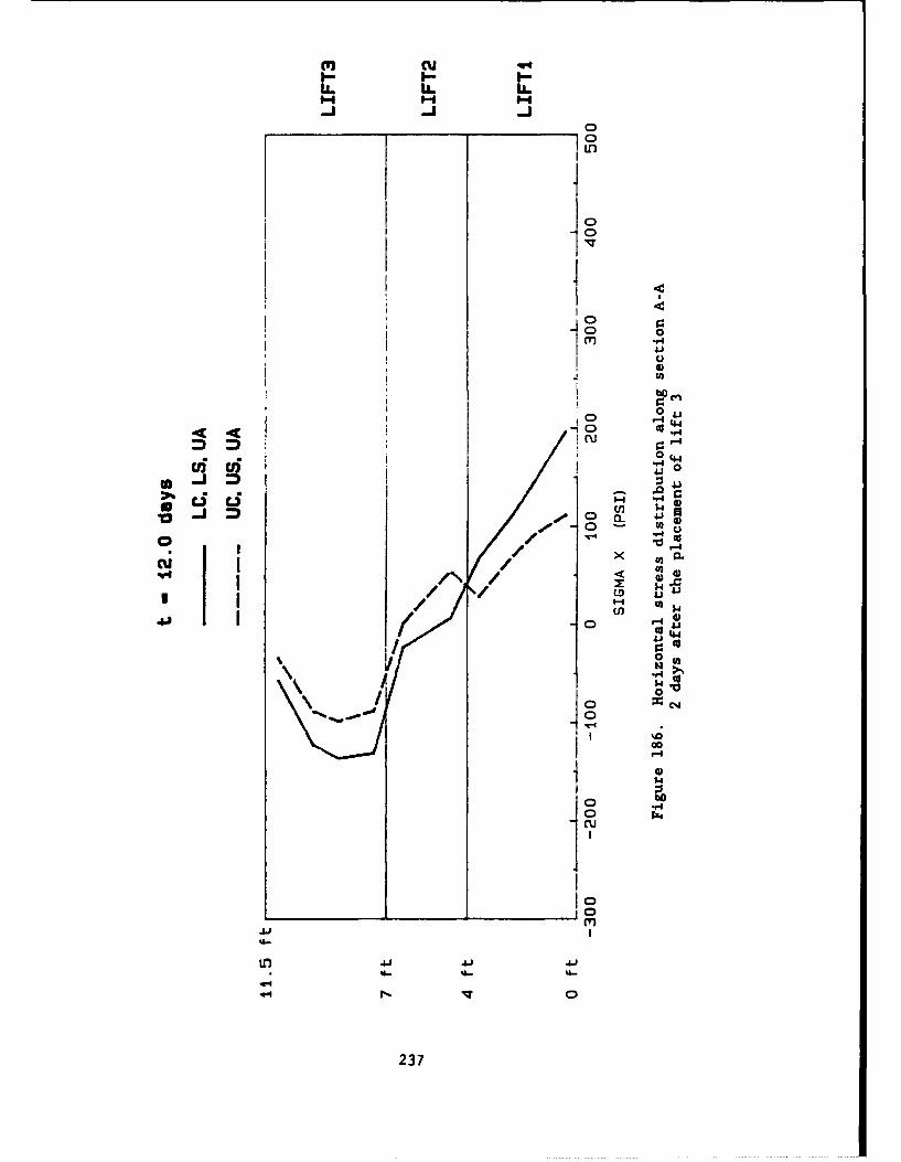
m cLIL LL U-
_ _ 0
- 0A
btoc
'-4 r-
C)
"U4 .
I~ 10
*1 a m
bO
(Zd
~~0
JGo r4
.aJ I
237
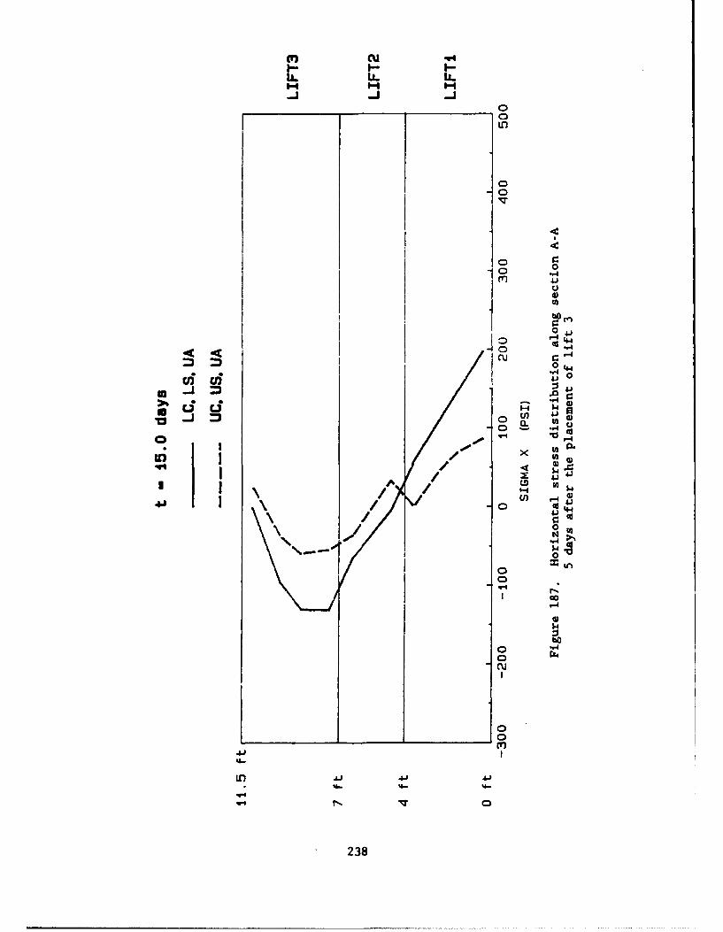
1-44 444I
CI ,
"0 400
in 4.)
0 10
(a )
04.
crco
u-ju
~I'h -* C 3 U '-
Q0LO0 4JA
238*.-
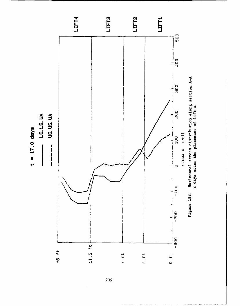
mn cLL LL LL IL.
-ij
O4j
-0 D0oo 44&, 4
* i ii Z '
"-4
r I 0 CL~J
xI IQ* 1'1
'-1
0 Il_ _ _ _ _ _ _ _N
2394
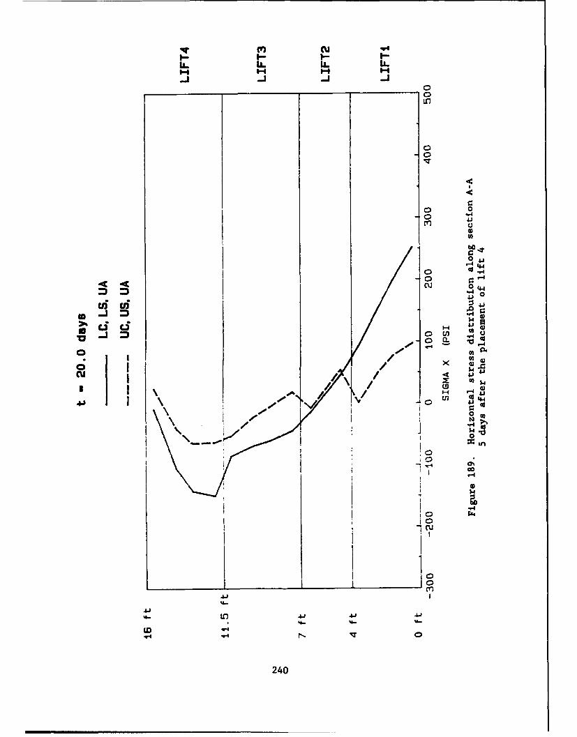
IL L IL IL
00
00
on U4)
0 41
"4 0
cui d4.
13 i o -En 4 )
0 ~rn0o 1l P.
Cu ,/\ ,cu D a
I .0
'-4
I00
'4-4
4-i4
240
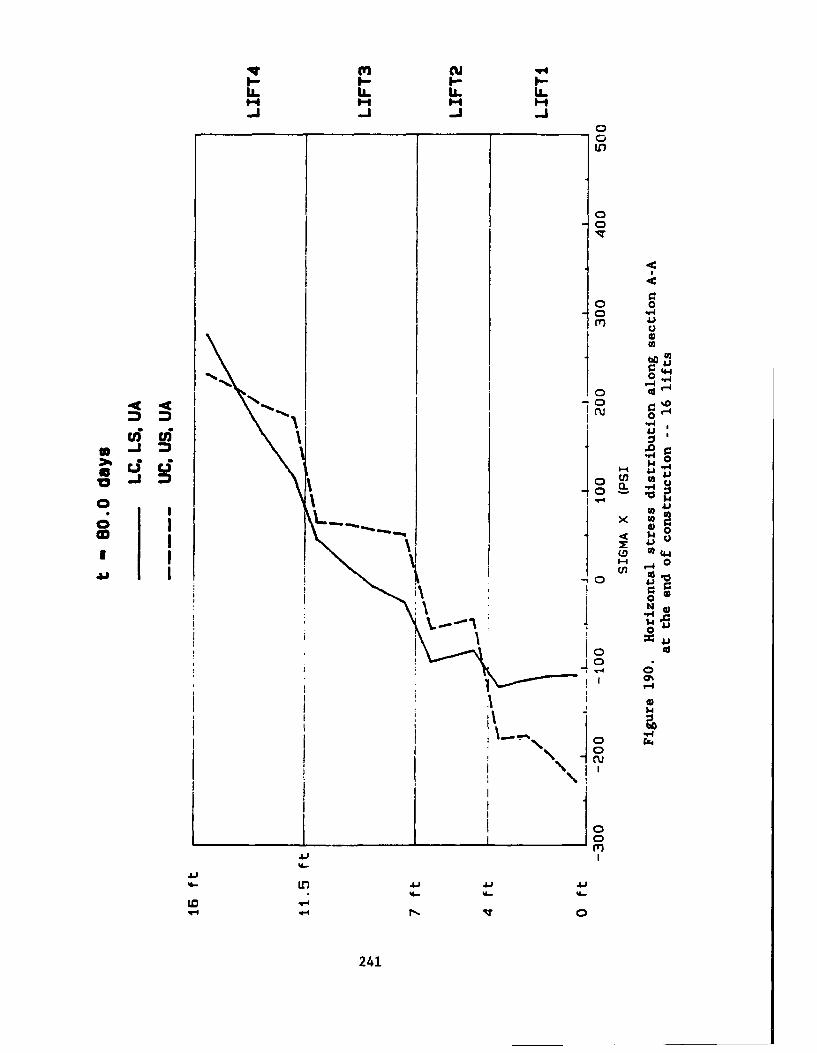
_____ 00 "
0.
o4 o
C.)
0 0
11~c3Li I :3
"4 0
02
"0 0
4.11
Nr 0
2414
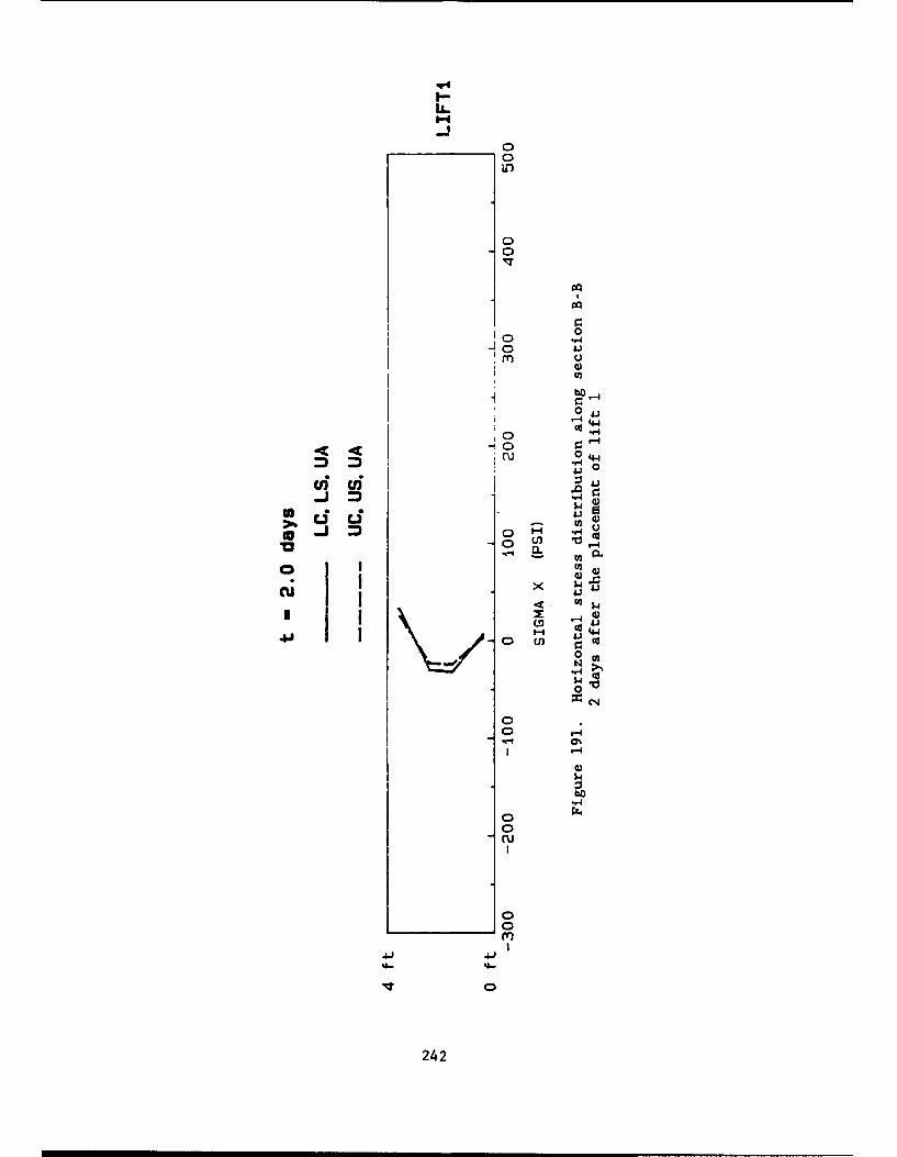
U.-
IL
000 "
-10
bH o
0 4,
4 4-0 -4 4
r 0 44.
cs Li 410 cd
-x w 41o I)* IA
4J0 to0 '
04.0%
bo
0mU
0
%&.- '4.-
242
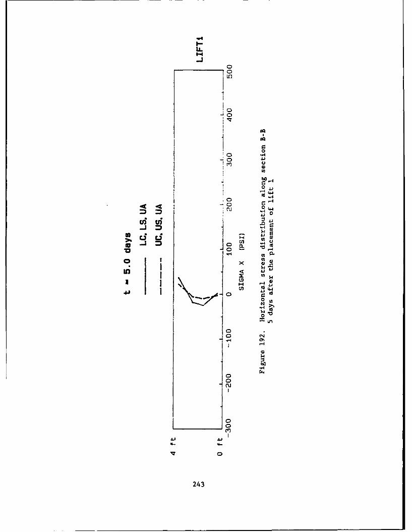
IL
0l
00C:)
m
-o-
0
-o- 44'CC -,
row-4
"40)
041
En -r
C3 -
0-o
CD 4
00oN-44
00
00
44"4
0
243
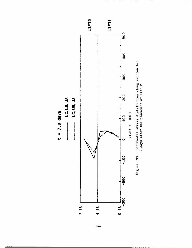
cu V4
¶00
s0 04
I~ 04.
I"-I
u~1n fo -4
4)0
I4
4104
14.0
0
2444
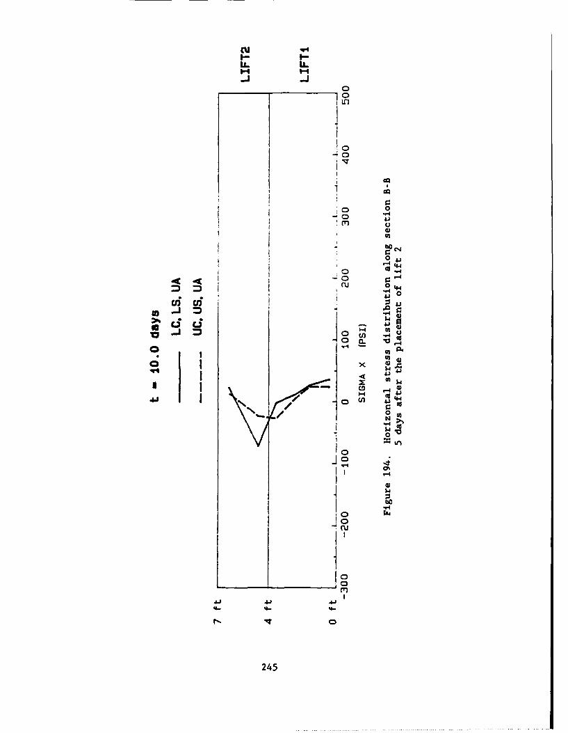
010
0
0 r
"4 0
1-4
o' 4ca
Ix
I, 'I
$4.
II
0b
I ~0 *~-V
245_ 1
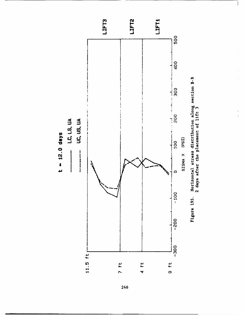
LL LL. U.
I-I1 q- -
'00-Coo
r4Ii -0
4$
xid 4) 0X 4j
W0 5
0
100
4-I4
'4-4
q-44
246
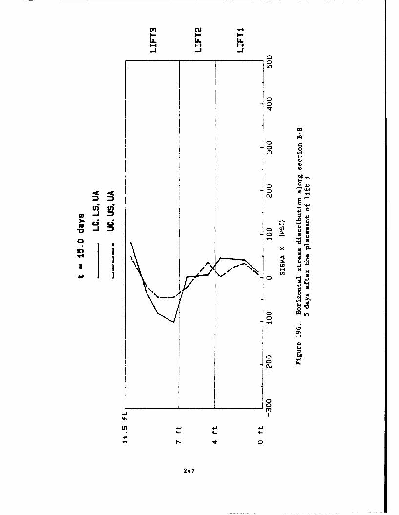
I--I
1 10-00
I 11100
0 t
C: c nJW Q
$ 4J
co 4
.44
.4-' I
247
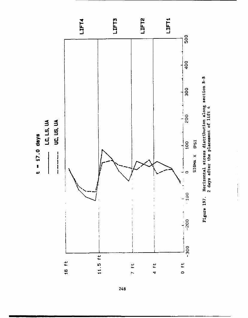
CU q4
0
10 04
"04
"0 4
uic 440
10 000
4J I,
Ln~
to 1-
m V-1
4248
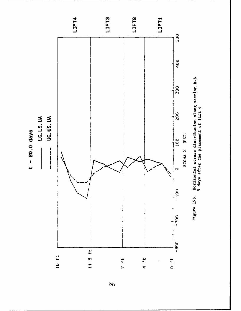
m cuLL LL U. IL
100
U))
Iobo0 -
*c ,
4J 41ow
"4 j,
a'SA)
cu 4)
D 41
(0 0
00
249
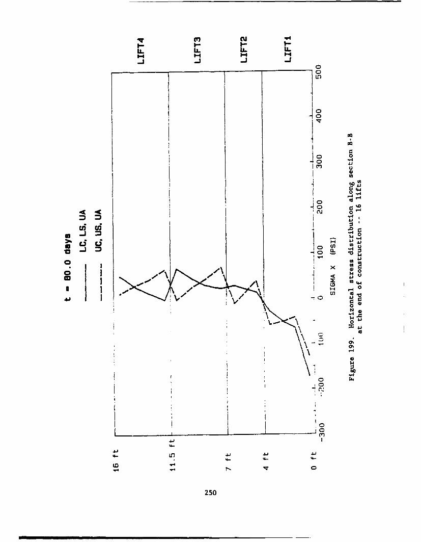
?-J
,e~J 0
r.)
0
00 "4~)41..
U;)
"40
'-4 ,
0 4
tt o
q.4~" x~
250
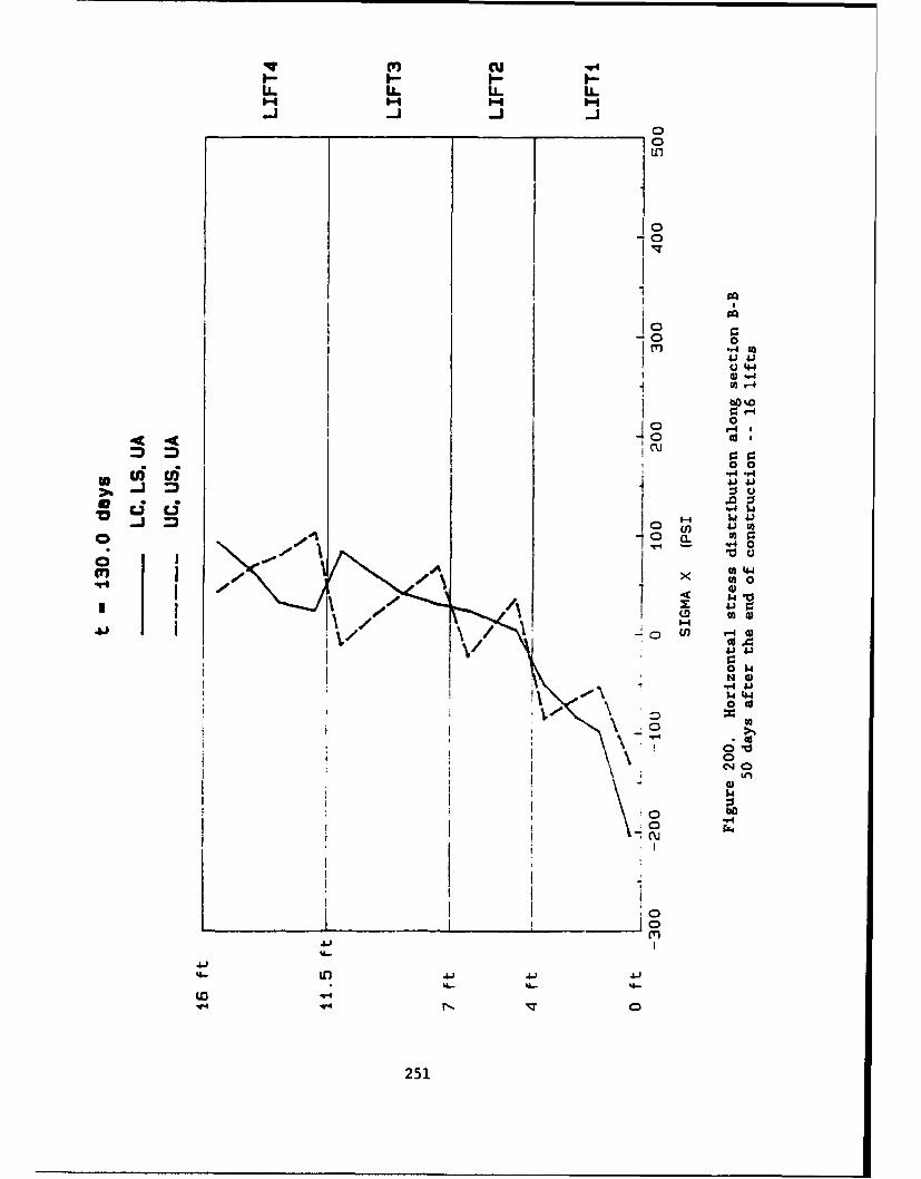
m, U.
00LO4
.r.0
.4. Ac c
0 00f Ed 4
"-4 00
.00
0Ico I
0 $4
0 CC)l
ru
.1251
are smooth within each lift. However, at many lift interfaces there is a
discontinuity in the horizontal stress that is more severe at later times.
The strain plots shown in Figures 201-209 clearly show that there is a strain
differential at the lift interfaces. Due to the difference in material prop-
erties and the nonhomogeneity of the lifts, residual stresses and strain
incompatibility might be expected. However, one would like to see these
diminish with time. At later times this seems to be most evident when the
upper creep and upper shrinkage material properties are used. Current inves-
tigations are being performed to try and interpret this phenomenon more
clearly.
156. As mentioned in the section on modelling, the top of the openings
are temporarily supported by multipoint constraints (MPC). The following is a
presentation and a discussion of the results related to the MPC and the model
used for the openings.
157. Figures 210 and 211 show horizontal stress and strain histories at
the bottom of the culvert. The sudden jump corresponds to the placement of
the lift closing the void. Through the investigation of the distributions,
shown in Figures 212-215 of the horizontal (Section B-B, Figure 181) and ver-
tical stresses (Section D-D, Figure 181) just below the bottom of the culvert
and also through the investigation of some displaced shape plots, (Figures 216
and 217), it is observed that once the lift closing the void is placed,
30 days--real time, the section to the left and below the culvert bends out-
ward. This mechanical action gives rise to the horizontal stresses at the
bottom of the culvert and mainly at the left corner. Both Figures 212 and 213
which are stress distribution through a vertical section below the culvert
(B-B) show the distribution as pivoting as if being bent. The distributions
are rotating about a point near the point of zero stress with increasing ten-
sion at the top and increasing compression at the bottom.
158. Figures 214 and 215 which represent stress distributions at a
horizontal section just below the culvert show an increase in the horizontal
stress following the placement of the lift closing the void. The vertical
stress distribution, on the other hand, shows that both sections on either
sides of the culvert tend to bend outward. The above phenomenon seems to be
related mainly to the incremental construction.
159. Initially, the two wall sections are nothing more than cantilevers
attached to the base slab, which are loaded by only gravity and thermal
252
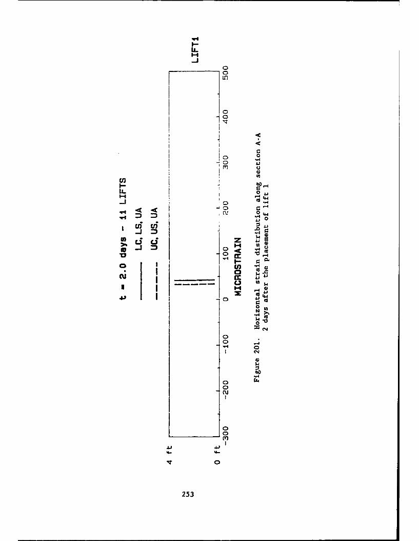
U-I
1-0
0010
cn bO
.4r.
U- 0
r4 4
0)0 4
in -n
"4-
0 wu..
41 4..
0)0
4J II0
114)
10
0c'J
'4-J
253
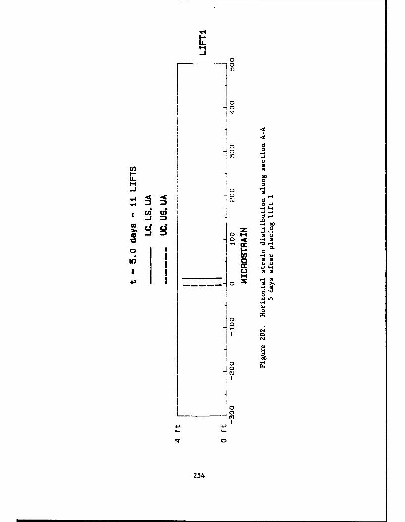
I-
00
-! 0
U)U
iL bo
I-4 0
.q-4 4 4 i"- -44
"4 b7-I
U) -, 3
,0
0~04 ",4c
1~ 4.(4.
cuu
00
2544
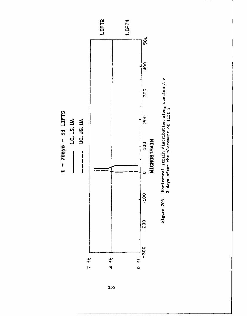
cu '
U. LIL
44
_____7 __ __ __ 0100
LLL
0 4
"*q 0
4 r 4,"4
:gC)
I-.0 U) 4 4to
04 $4 4gcicS
0 towcu14 .
00
C-4
4)
ob0
0
255
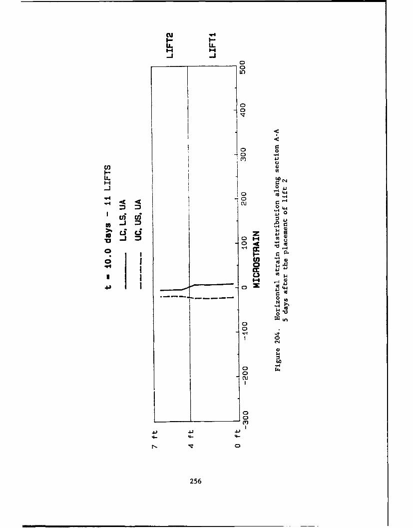
cu 'U- L-
LO
0
0 0
0 "
0 4
00
q-4 0)1>1 c'J o, z 41
.10jC) IO
o -4)
'44 1
r 0d
0
0
0 40
0
256
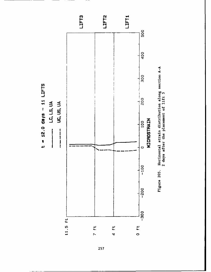
LL LL. IL
0U-,
10 0
0 4
0 I- 4
41 0
"04.
"o u
cu En " 4*14 0 t
44J
rtow
00
00
C)l
ob
0 "
sJ I
'4-
m1-
"-I 0
257
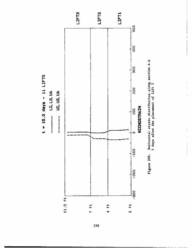
1LL U. IL
-i -j
0
0
0) 0
LL U
0 0
-040'4 <4
'cd ui0
o ,0 0
4'4r4.
U)
00
4-, I
'4-4
'-440- 9x0
258u
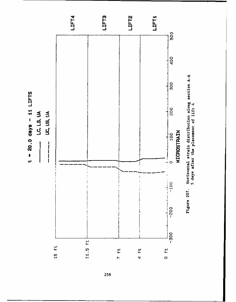
P1 ~cuI.LL 1- I- I
0
U))
LL
ohI 00 ~4104 `4 4.4
'cdc0 r-4.o
"0 4
o j M n IsCur 4
4.1o "4 4)-r c~
FA 1Nd4
I I -r.
4J )4-4
4-)4
N 10
259
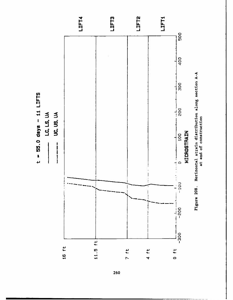
cu
U- LL LL L-
00
0 00 "
U)U
00 Ccd
"4 :
0 0
1 00 cc 0
-. 1- - -I
0 w
m4-,
4J- U, 41J4'4-r '4-'
(00
2600
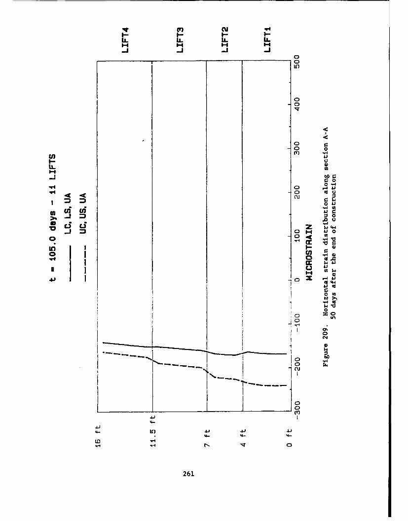
OJ q4
LL ILILl
0
00"
0 1
o V"U) U)
V- 0
Z 4q4V 0
".4 4)
20( goM w
IL, 1-*
0 V
0
'44-
261
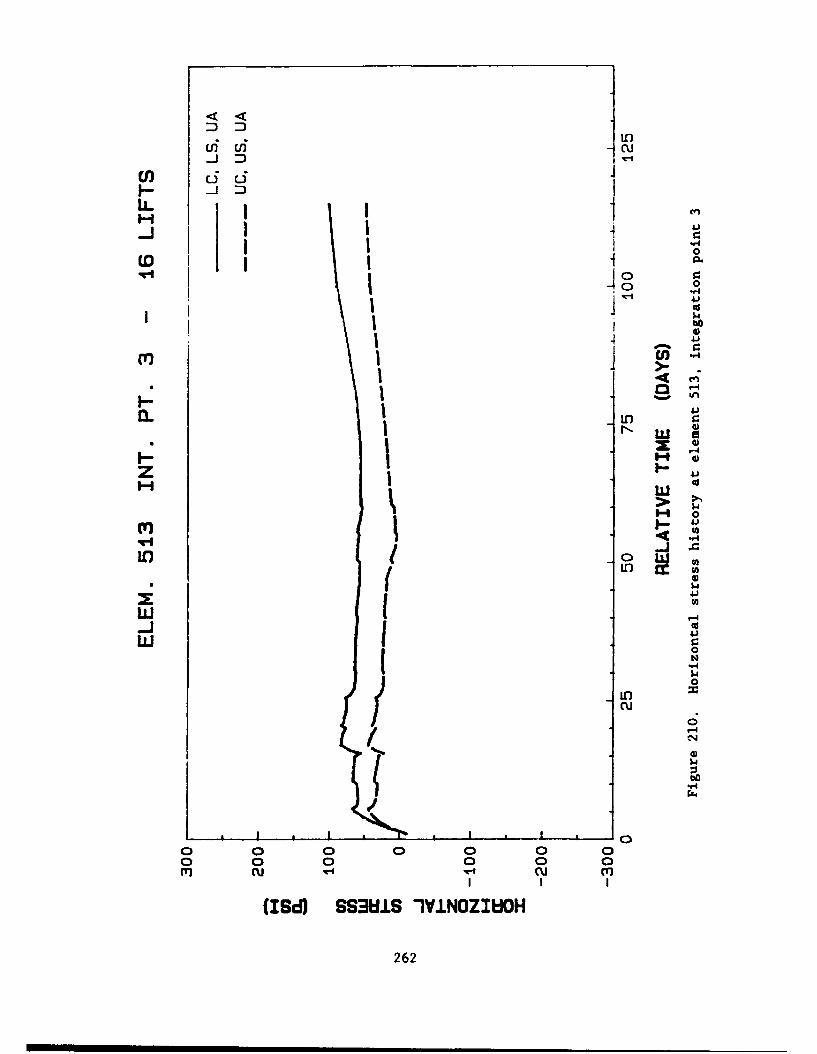
LL1
I 0
j 'a
I bo
ccv)
LM
I4- 1 In 'a
~~r4
* 1 0mI
I U)
w
0
LO
-40
00
II I
(ISd) SS3W.S 1V.LNOZI~hOH
262
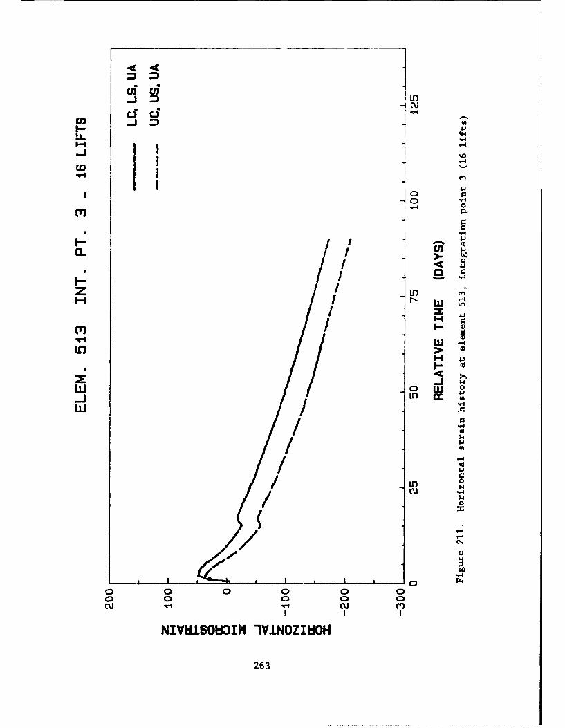
cuci cs
LL w14 r4
F-J
CDD
'4 1w In
Nw>- 4)
W 0(I') 1-
qi w 04
If) 1 >
-4
0
r4C14
0 0 0I I
NIVU OWINIVINZIHu
2634
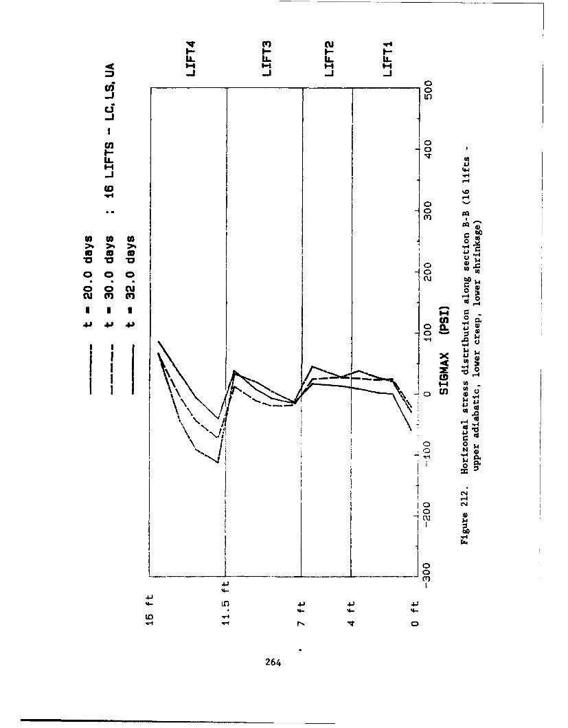
I---I-I
44
cd _ _ _ _40
4 0
Cn ~0cu m r-CdLr
x- 4J 4"'
-v-CD 1
EnI
%Ali V
100
:v'O
4.)4\O 414-Il 4-
2640
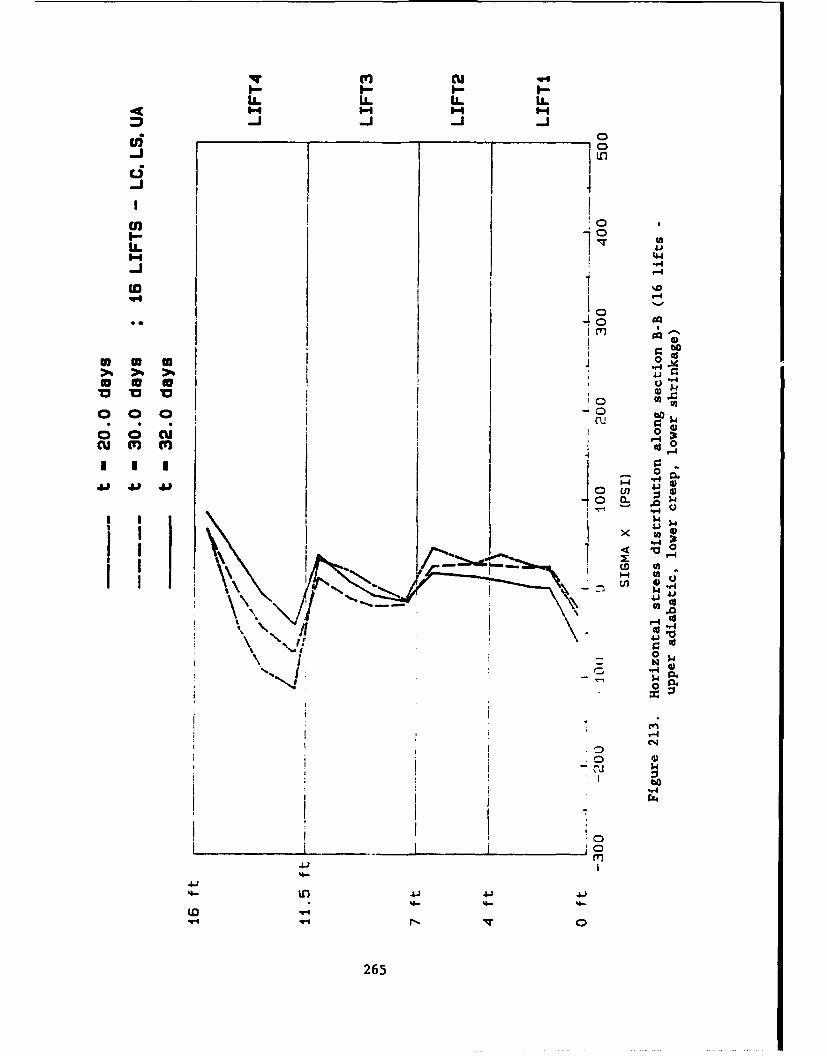
m cuI--J
.44I 0
-I1
.0,ro4
00W0
44 $4.
4J 4J U 4w 41U
*10-r4
\~i **~-o
\\, /j0
0 (
Ila,
C14E
'4-4
4-,4
"41
265
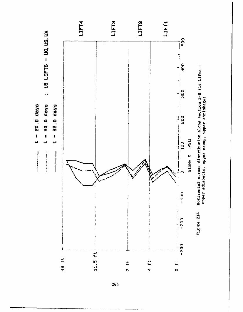
ui 0
LL~
cir
q.)
q4 I
cu m c CO o
I C'0
I I I III~ I
4 14
ICd
0 3 4
ii . 4
I r4'-I
I IN
I IT
266
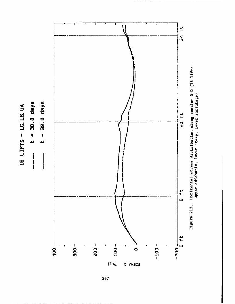
m
"4I
I (4"'
I qII"I$
U) '4)
00 0cs5c 0;C ur
U) 4 ..114J)
IL wI~j 10
I ~4J
"4j4
$4-- - - ---- 4 - - - - - - - -
C..4
0-
o o 00 0 0 0)o0 0 0 0)
Vcu cu
(ISd) X ~VWSIS
267
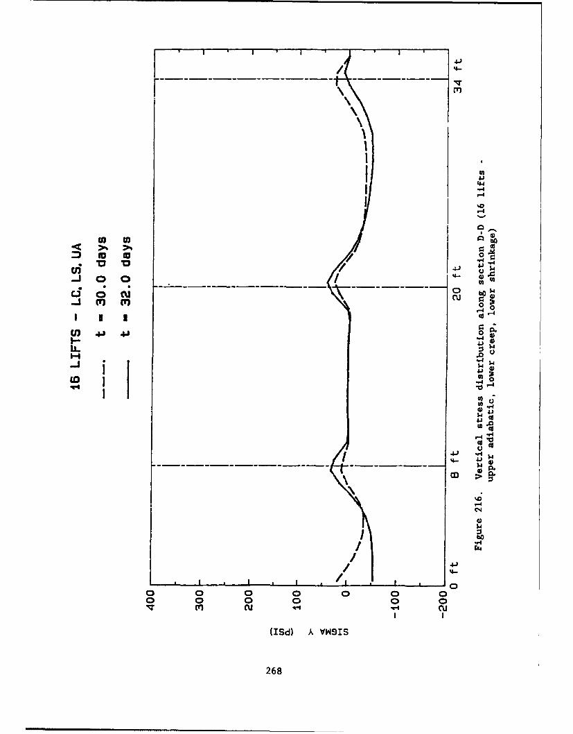
4-,
/ 4= 4
4.1
_j 4)-
4 0
r.-I
/ 4- 4
4~" $4m
Cl)4 .51)5.-- - - - - - -4 P4J0
.44CC-
-4)
0
I5-
(Isd) A VWSIS I
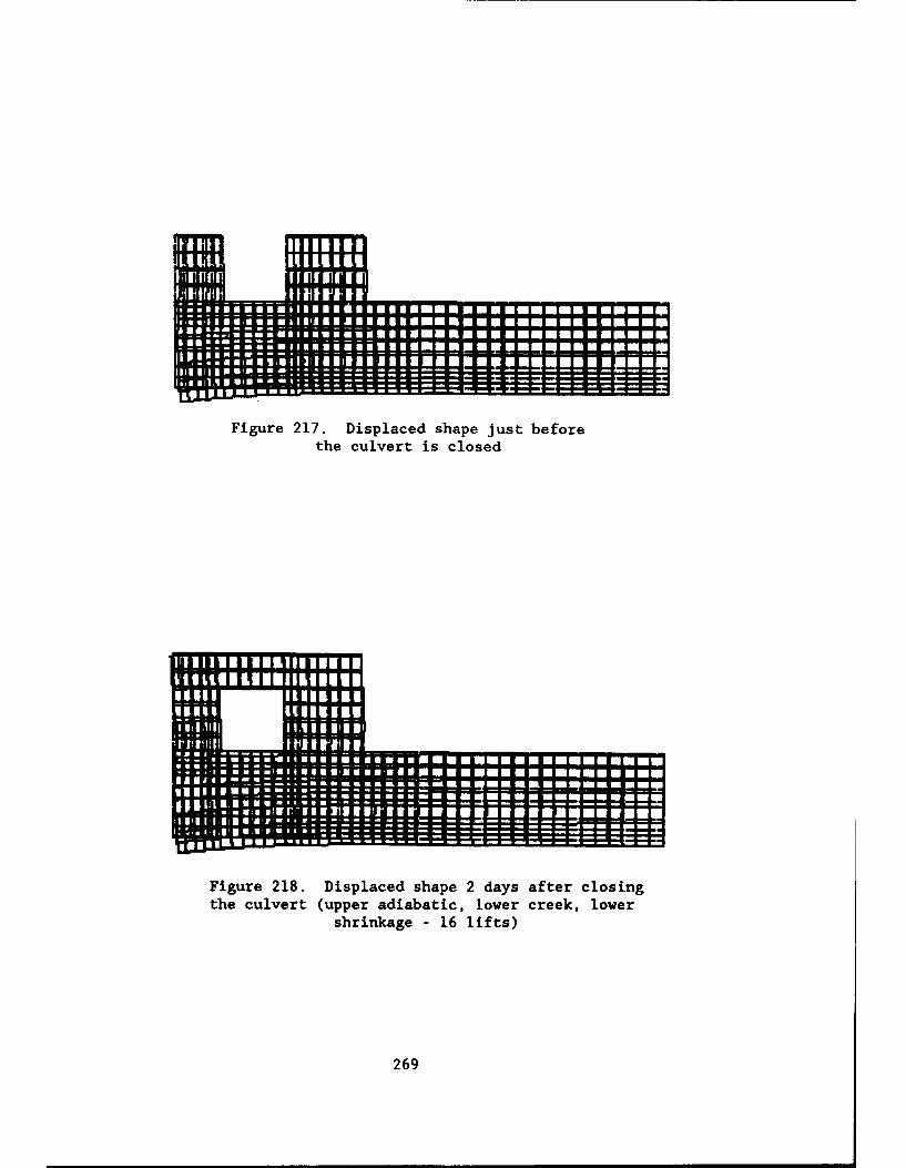
Figure 217. Displaced shape just beforethe culvert is closed
Figure 218. Displaced shape 2 days after closingthe culvert (upper adiabatic, lower creek, lower
shrinkage - 16 lifts)
269
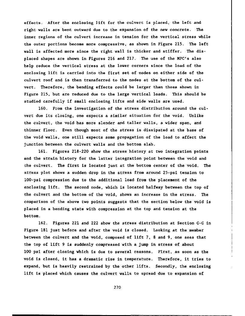
effects. After the enclosing lift for the culvert is placed, the left and
right walls are bent outward due to the expansion of the new concrete. The
inner regions of the culvert increase in tension for the vertical stress while
the outer portions become more compressive, as shown in Figure 215. The left
wall is affected more since the right wall is thicker and stiffer. The dis-
placed shapes are shown in Figures 216 and 217. The use of the MPC's also
help reduce the vertical stress at the lower corners since the load of the
enclosing lift is carried into the first set of nodes on either side of the
culvert roof and is then transferred to the nodes at the bottom of the cul-
vert. Therefore, the bending effects could be larger than those shown in
Figure 215, but are reduced due to the large vertical loads. This should be
studied carefully if small enclosing lifts and side walls are used.
160. From the investigation of the stress distribution around the cul-
vert due its closing, one expects a similar situation for the void. Unlike
the culvert, the void has more slender and taller walls, a wider span, and
thinner floor. Even though most of the stress is dissipated at the base of
the void walls, one still expects some propagation of the load to affect the
junction between the culvert walls and the bottom slab.
161. Figures 218-220 show the stress history at two integration points
and the strain history for the latter integration point between the void and
the culvert. The first is located just at the bottom center of the void. The
stress plot shows a sudden drop in the stress from around 25-psi tension to
100-psi compression due to the additional load from the placement of the
enclosing lift. The second node, which is located halfway between the top of
the culvert and the bottom of the void, shows an increase in the stress. The
comparison of the above two points suggests that the section below the void is
placed in a bending state with compression at the top and tension at the
bottom.
162. Figures 221 and 222 show the stress distribution at Section C-C in
Figure 181 just before and after the void is closed. Looking at the member
between the culvert and the void, composed of lift 7, 8 and 9, one sees that
the top of lift 9 is suddenly compressed with a jump in stress of about
100 psi after closing which is due to several reasons. First, as soon as the
void is closed, it has a dramatic rise in temperature. Therefore, it tries to
expand, but is heavily restrained by the other lifts. Secondly, the enclosing
lift is placed which causes the culvert walls to spread due to expansion of
270
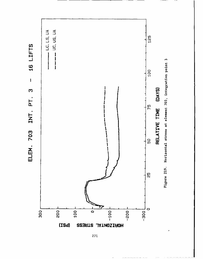
Eliui U-cu) riD
(.0.0
.4-
ý4-
zz
I~03w NI,-
ob
0 0 00w 0 )
I I
2714
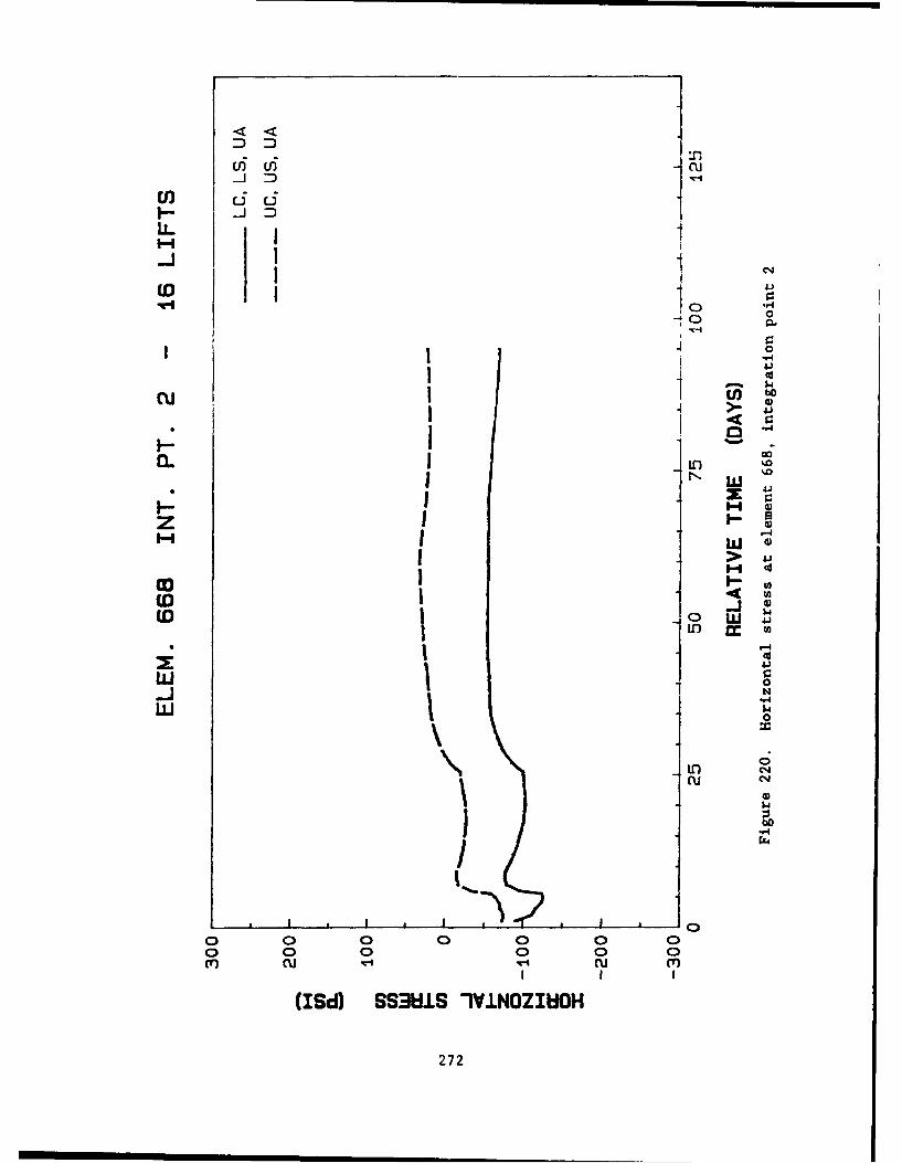
I--i -Pu1
(D-0
C)4 0
(N 1LJ
00
LOU
3E jr
wW
tow
ui 0
00
m nC1SS3UISc 1V.NVIO
272
:D VU) ui Ei -1 U
LL. LS Li--J 14
I - 41
I 0"-441'U
ý4.
II U)
44
'41
CD >-,(D ~04
(00
I JJ
"4J
00
I -I
NVL HO I IN I IO
273
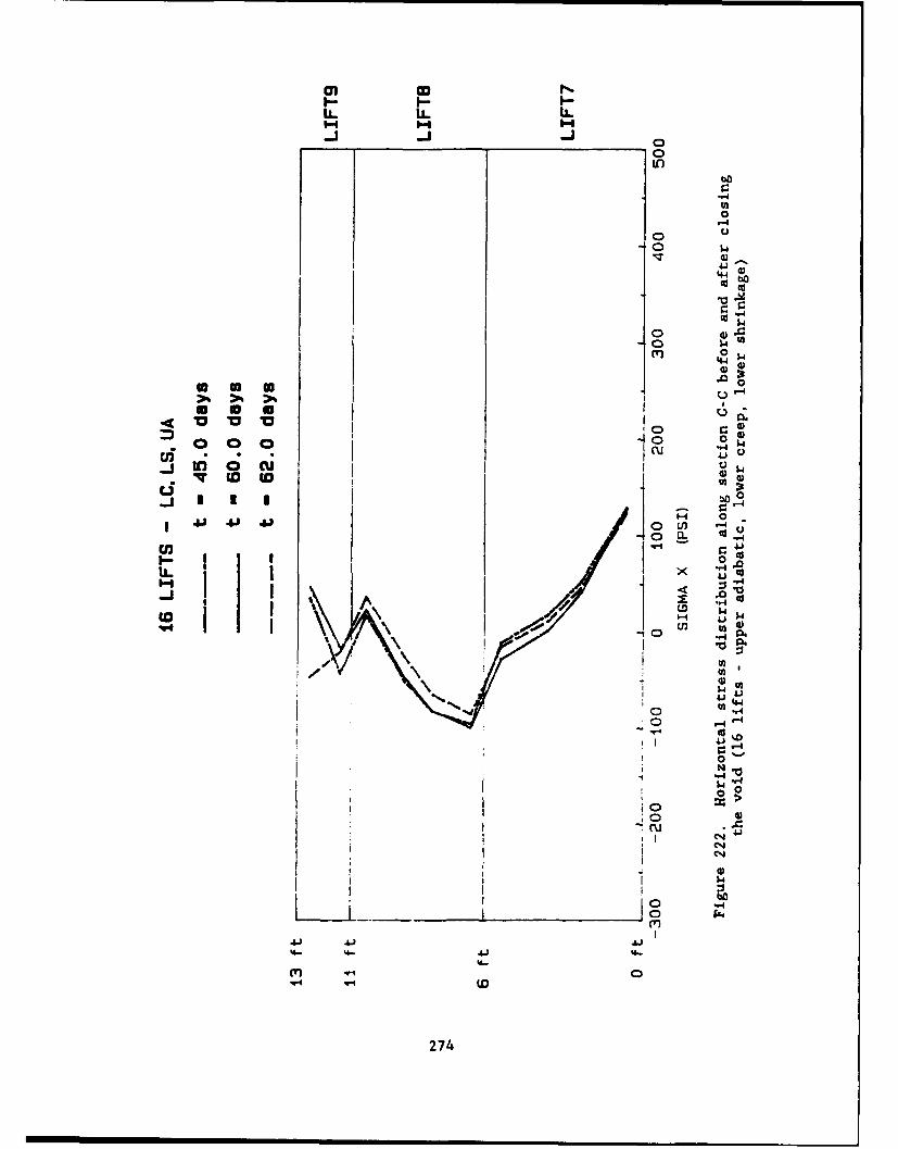
I---
bo
CA0
0 14
ok
ot0v
* 44 14~~4)
* U Uj a5
v It) CU*4
!o0~~~g ý44
0
"J 4J
0 c
IL 0
4-IW 44
'4-4cvi ~%
(00
2744
the lift, placing the intermediate member between the culvert and the void in
a slight bending situation.
163. Figures 223-226 show the horizontal and vertical stress distribu-
tions at a horizontal section just below the void, and the displaced shapes
before and after the closing of the void. The displaced shapes show that the
left side of the void is displaced to the outside and as expected downward
while the right side has hardly moved. The vertical section to the right of
the openings is much stiffer than the left. Figures 227 and 228 show the
effect that closing the void has on the stresses below the culvert. Closing
the void affects the left corner the most since the left wall is the weaker
section as far as lateral restraint is concerned.
Comparison Between the 16- and 11-Lift Schedules
164. To compare the two lift schedules, the results are grouped as
(a) horizontal stress history plots of nodes in the slab, (b) horizontal
stress history plots at the lift interfaces, (c) horizontal stress history
plots at mid-lift locations, and (d) vertical stress history plots at outside
edge nodes.
165. Figure 229 shows the locations for which the stresses are pre-
sented while Figures 230-238 shows the stress histories. Within the slab (see
Figures 230 and 234), the difference between the two lift arrangements is
small with the exception of points close to the center line. It was explained
earlier that the chamber floor arches as more loads are added to the wall
sections which results in high tension at the top of the slab and higher com-
pression at the bottom as seen in Figures 230 and 234 during the 11-lift con-
struction. The latter two figures show that the higher stress is only due to
the heavier lifts and earlier time of application. At later times the
stresses coincide. For every additional lift, the 11-lift curve shows a
higher jump or increase, due to the larger lift heights.
166. At several of the boundaries, the difference between the two lift
plans is noticeable (see Figures 233, 235, and 236). The highest difference
occurs at the bottom of the void and is shown in Figure 236. The maximum
horizontal stress for the 11-lift is about 180 psi; whereas, for the 16-lift,
it is only about 50 psi. This difference is primarily attributed to the large
thickness of the lift just below the void (lift 7). To explain this idea one
275
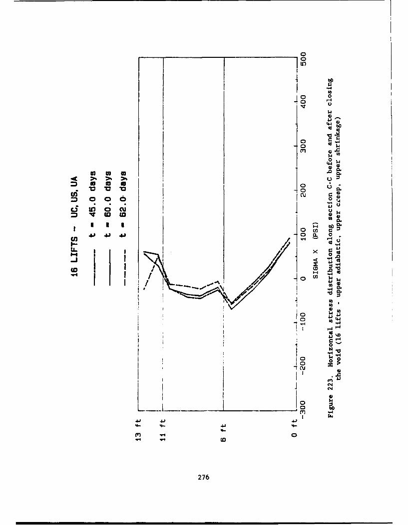
:30
110 $4
m 0 0 0 ! 0.s . C ýVU D
~ 000tn r.c
I-- d"/1 ii4oE/$
K ~ \ ON*0 IN a
ICdII4
7 CU
I j CýJ
'4-4
276
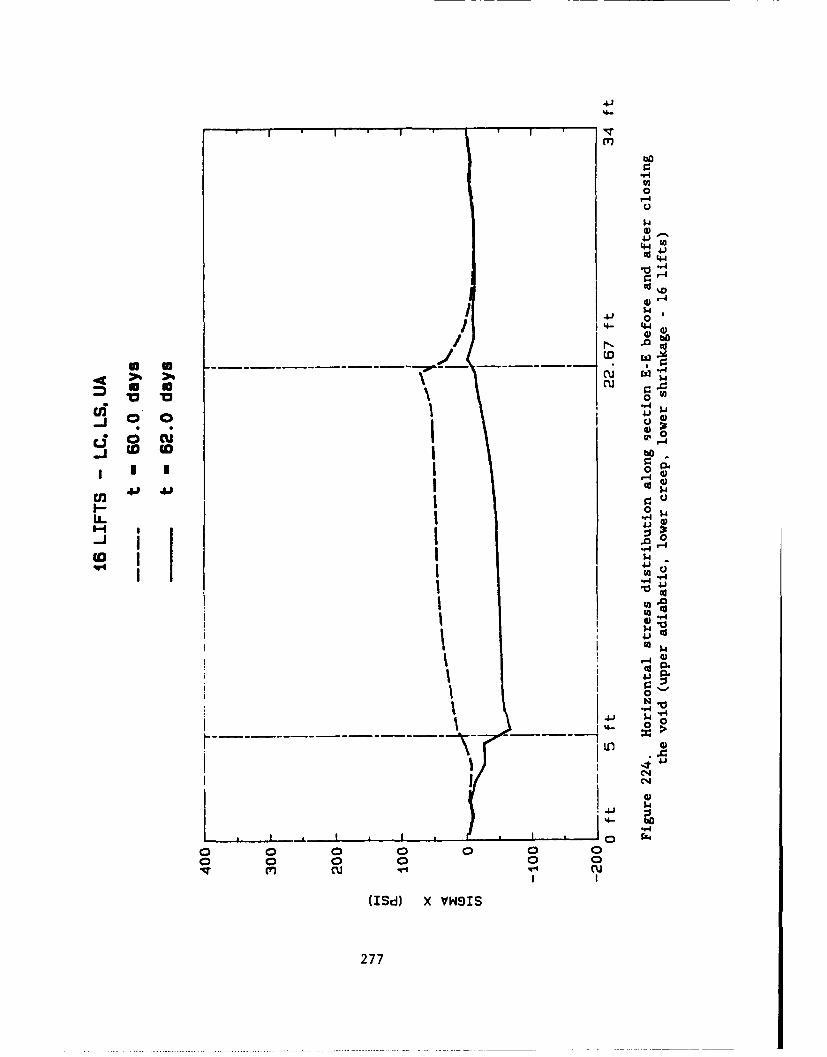
4J
0)
f41
0)
cuS Su
0041 4)
000
I *0
ciOd-0
L i "4 4
4~ jrII- owU-1 IM
I ~4J
~0)
I1 >
In 0
C14 4
C.,'
K )
277
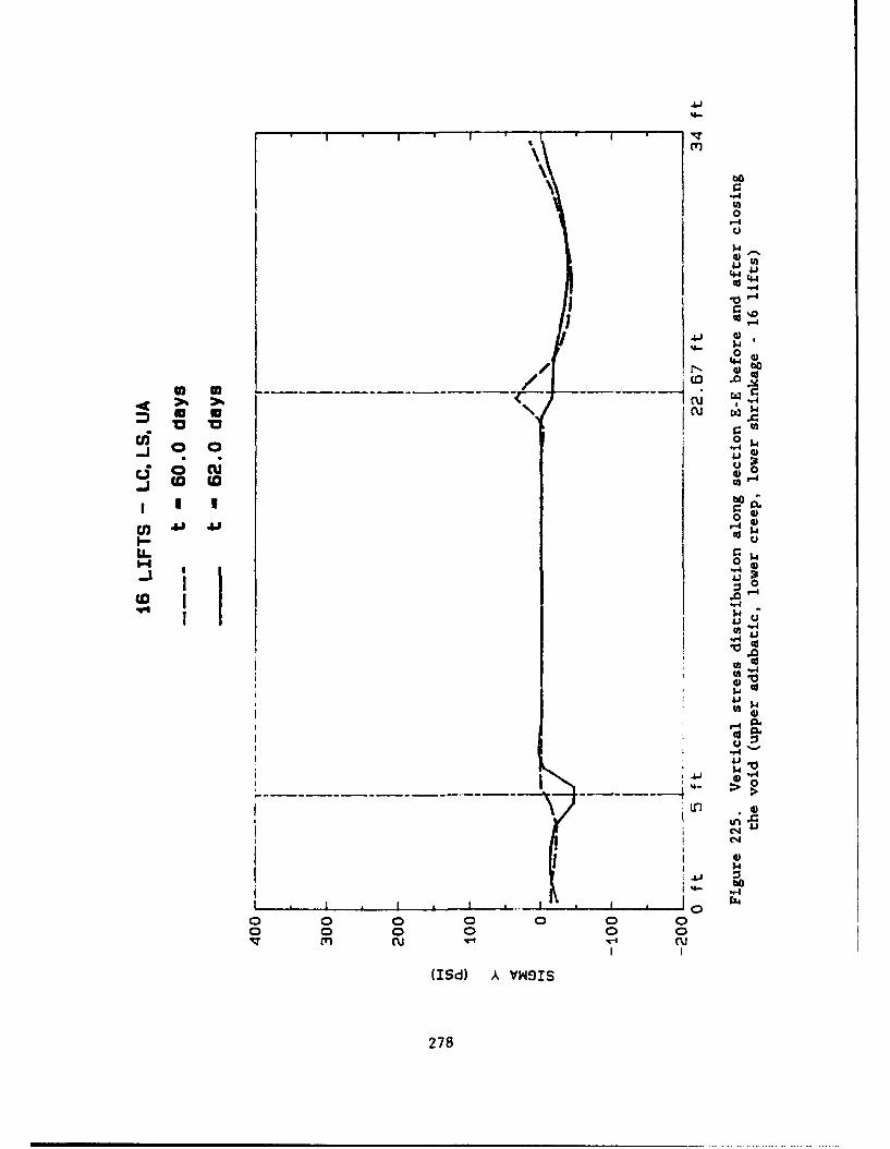
"4-
00
$4J
IGi/ c~41
/4
10 ) -o
cli
.0
.0
0 ),
j D
f I 0)
"-4
m~4 ru"-I Il
(I~~d) A41~9
278d
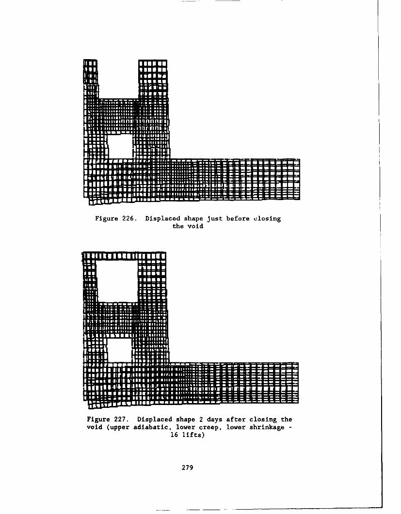
Figure 226. Displaced shape just before closingthe void
Figure 227. Displaced shape 2 days after closing thevoid (upper adiabatic, lower creep, lower shrinkage -
16 lifts)
279
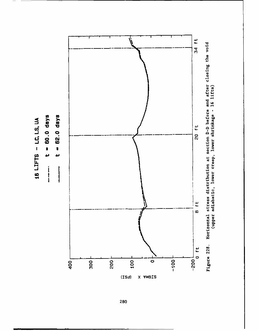
"4-
M 0
bO
"-4
0
$4 '0) W
'-4
Cd r
"~4b
#44
0 U)
41 XU 00
a) in-
)41 .61
I-4
0 u
"-4 0-
-W-4
I-4
0
"4-
0-,
a * I * I I * ~ 04
Cu ri cu "
(ISd) X VWSIS
280
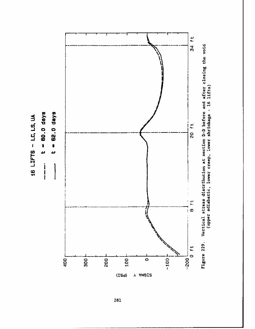
mr 0,,4)
bOU01-4
4)4-44 "-1ca -4-
ow)S 'bO
1010 0 1-4
ci w 0 0 r0
00.-
IU .- o
r.. U-
IL/
1-0 ~.4)
,.-i
L1 0
.00
"4 p
4-)-.0 0
m q-4r-4
4- m
(ISd) A V1HBIS
281
lift 16 lift ii
|_: "_lift 154lift 10
lift 14
-~ ' f , i t 13877-4 - lift 9
lift 12
Si f t 11i __ift_- lift 8
706-1.-3 lift 10- lift 9 lift 7
' lift a
lift 7 lift 6
lift 6lift 5
513-4 I lift 5 537-4
I~~~~~~~~~~~~ 1 If, I I I 41111111I it 3I I I I I I 1 1 1 I I I I I I I I I I I lift 2-
387-2 285-2. 411-2
Figure 230. Selected elements for horizontal stress comparisons
282
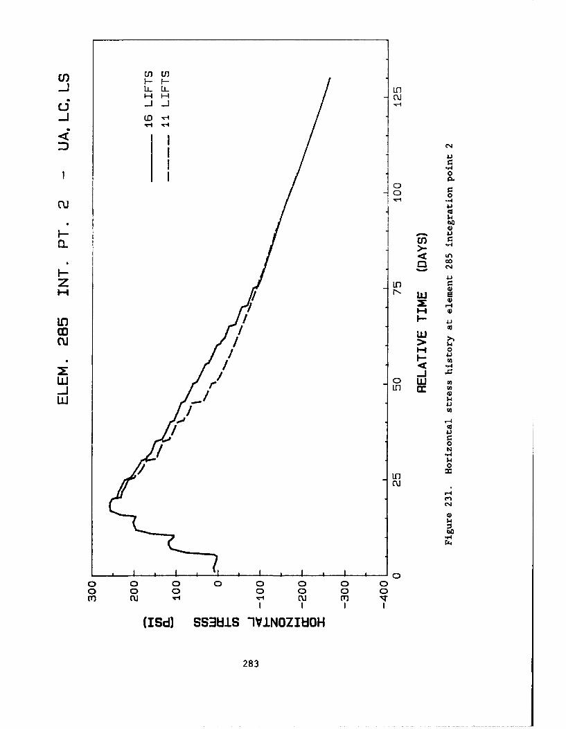
U, w
I 14
0
00
1141i
z In-3 N 0
04
00 w0
cu > ~-I 0
/L 0 WJ.
0LiiI "4)
0
4)i
/P00
0 0m clu u m u
I I I I
(I~d)SS381 -IVICvI80
283%
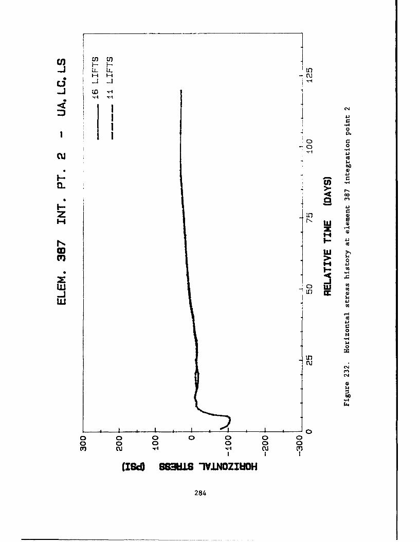
I
00
.41cu CbJO
1-* 1
000
> 44
I~4.)
r-4
03
~j~
.r4
284)
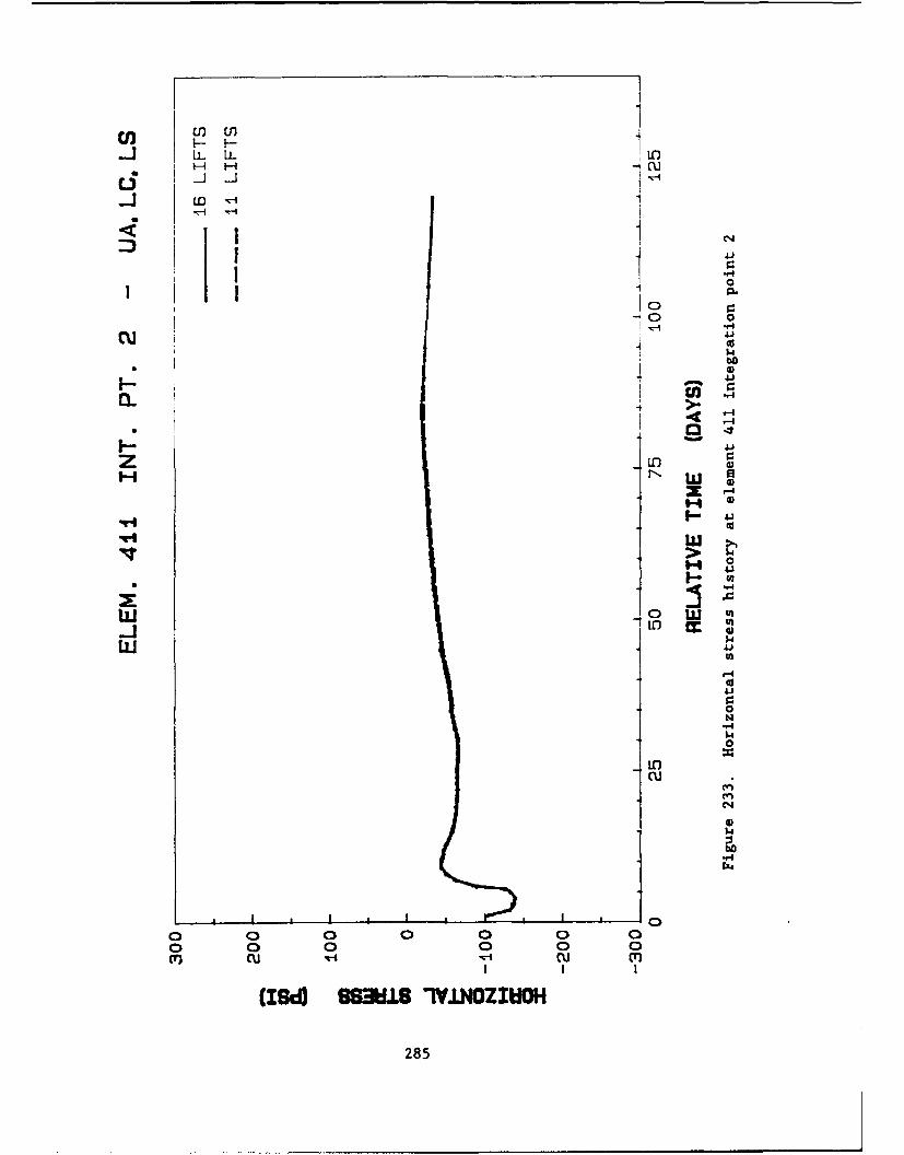
En t
Li- LL LO
""
L1
0
-o) 0
bC
4r
I 4JJz I'-,34> $4 L
0
0Ww
0
w C4J4)14"4J
00
cu cu(I~cD883MS IVIOC'W
285,
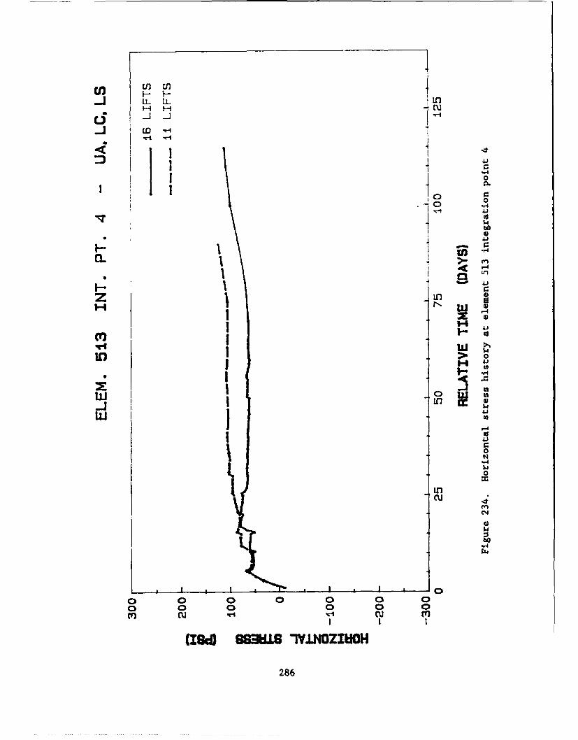
LL LL l
to
10 0.100
-o0
14)
Z 1 10
r-4
ILI 1U )
11r4-
1 0N
'.40
Inn
4)
1z4
0
SM GI IMI I
286
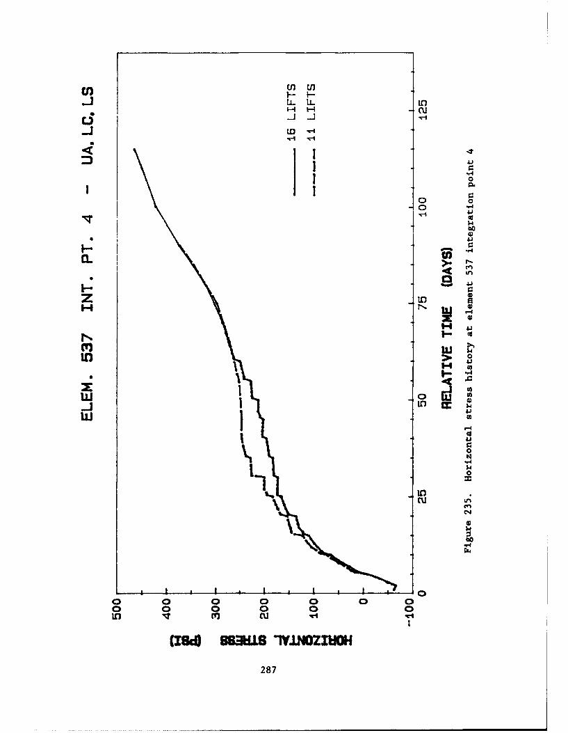
Cl) )- wLL L Lr
-4I- 0 U
ab
1 01
0 04
03
a. U)
z 0M0
If))
0 04 0
0 0 Cw Iu(I" S US -ww4.)
287I
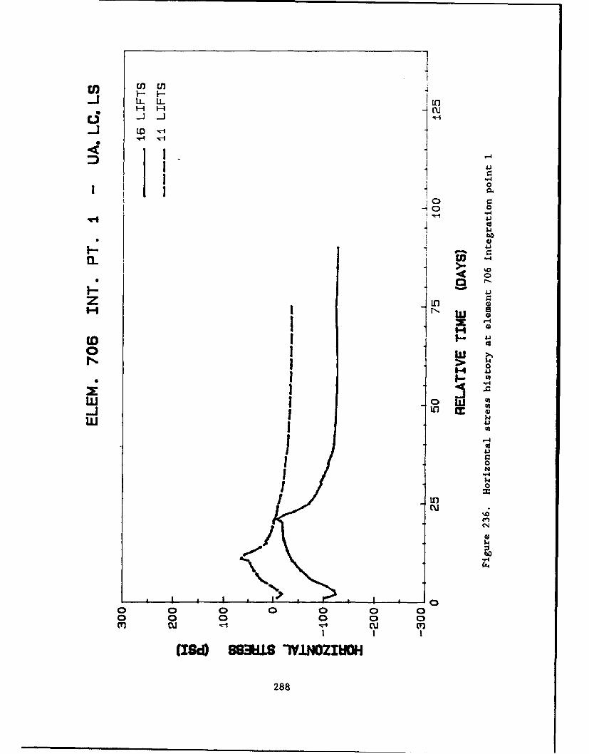
CD 4
4:4
00
w -0
ww
I-. o0~0
$O
0 0 0
in cu cu in-
UJ ~ QS8U W.NZW
288.
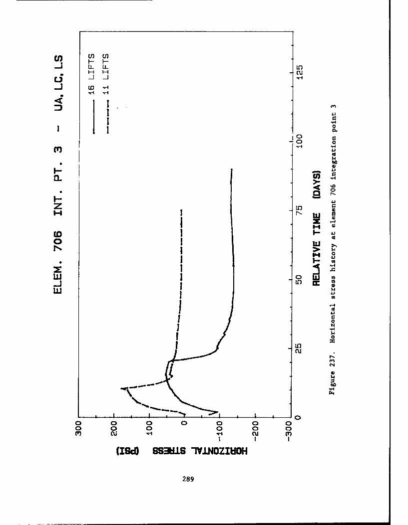
En HI-
LOOd
0
4 01
%0
I 1~4.4 10
0
I 4)
$4.
I 0I N
I 0
II
0 0 0
289.
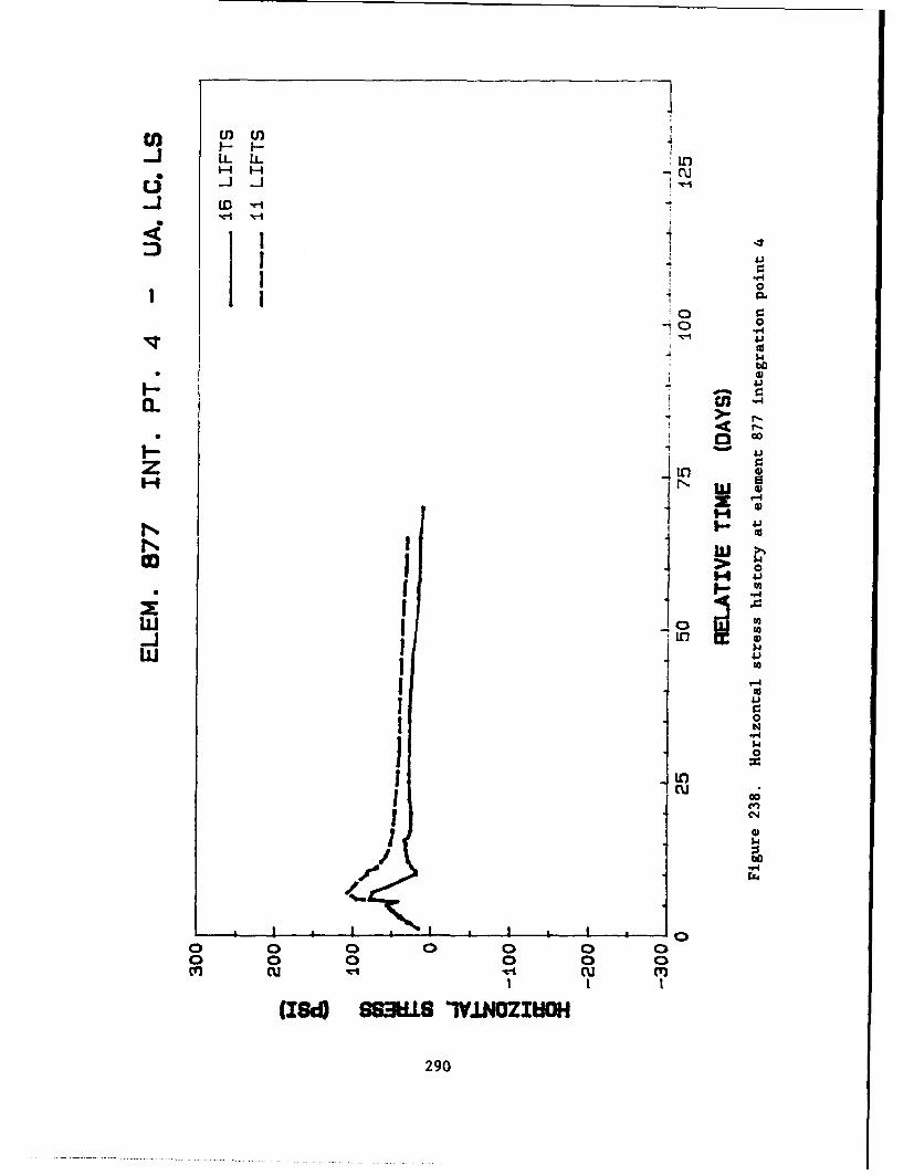
U)CU
41
ý4
44
*i 41
0~0* '-0
*C
0 1ac cu-4 4
(I S ISWGZH
w290
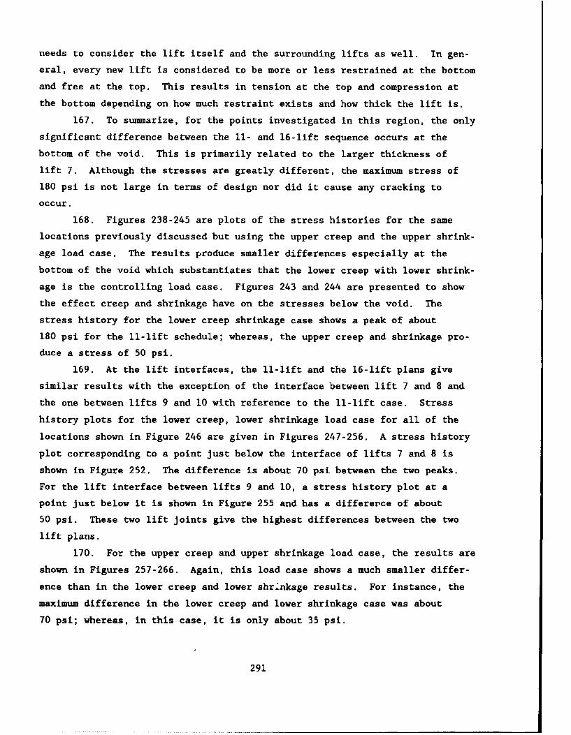
needs to consider the lift itself and the surrounding lifts as well. In gen-
eral, every new lift is considered to be more or less restrained at the bottom
and free at the top. This results in tension at the top and compression at
the bottom depending on how much restraint exists and how thick the lift is.
167. To summarize, for the points investigated in this region, the only
significant difference between the 11- and 16-lift sequence occurs at the
bottom of the void. This is primarily related to the larger thickness of
lift 7. Although the stresses are greatly different, the maximum stress of
180 psi is not large in terms of design nor did it cause any cracking to
occur.
168. Figures 238-245 are plots of the stress histories for the same
locations previously discussed but using the upper creep and the upper shrink-
age load case. The results produce smaller differences especially at the
bottom of the void which substantiates that the lower creep with lower shrink-
age is the controlling load case. Figures 243 and 244 are presented to show
the effect creep and shrinkage have on the stresses below the void. The
stress history for the lower creep shrinkage case shows a peak of about
180 psi for the 11-lift schedule; whereas, the upper creep and shrinkage pro-
duce a stress of 50 psi.
169. At the lift interfaces, the 11-lift and the 16-lift plans give
similar results with the exception of the interface between lift 7 and 8 and
the one between lifts 9 and 10 with reference to the 11-lift case. Stress
history plots for the lower creep, lower shrinkage load case for all of the
locations shown in Figure 246 are given in Figures 247-256. A stress history
plot corresponding to a point just below the interface of lifts 7 and 8 is
shown in Figure 252. The difference is about 70 psi between the two peaks.
For the lift interface between lifts 9 and 10, a stress history plot at a
point just below it is shown in Figure 255 and has a differerce of about
50 psi. These two lift joints give the highest differences between the two
lift plans.
170. For the upper creep and upper shrinkage load case, the results are
shown in Figures 257-266. Again, this load case shows a much smaller differ-
ence than in the lower creep and lower shrinkage results. For instance, the
maximum difference in the lower creep and lower shrinkage case was about
70 psi; whereas, in this case, it is only about 35 psi.
291
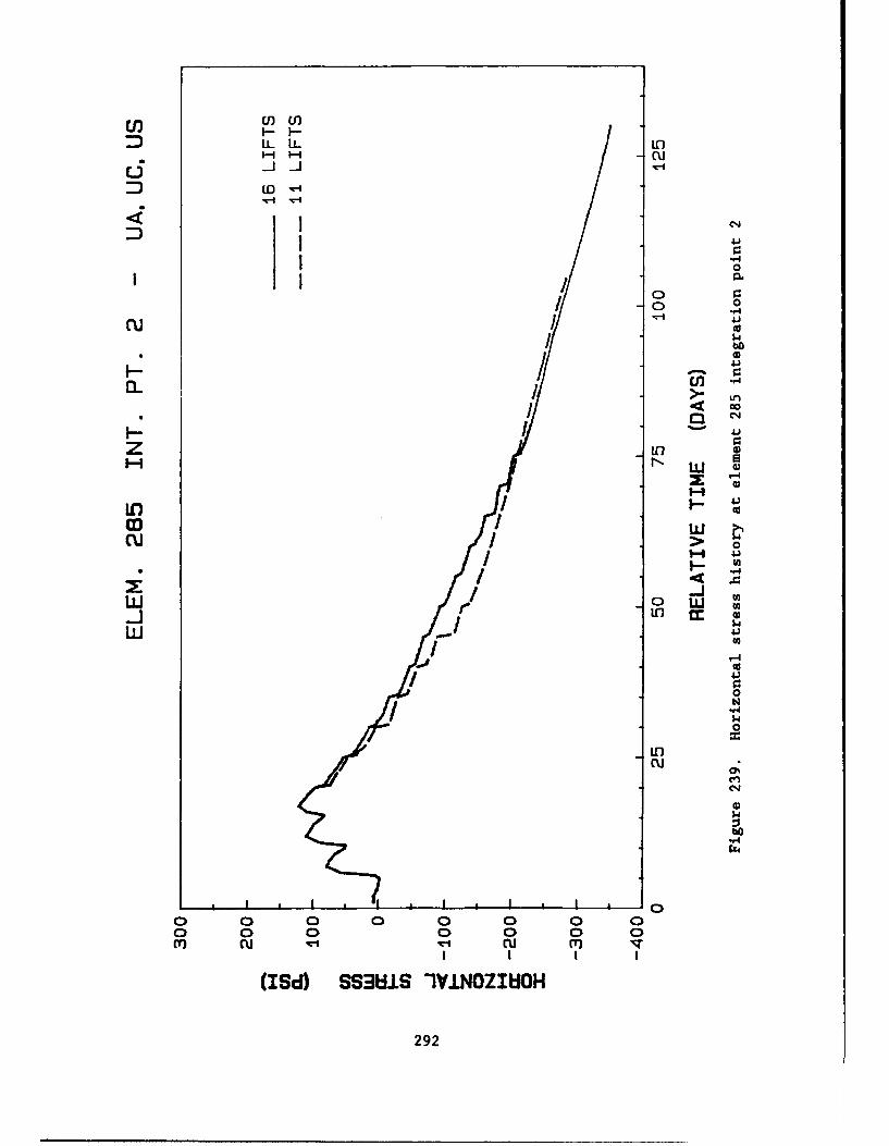
cn'
11
1 / 0/ 090
co II -t.
I- I4
0N-N
co uCU /4
0 0 0 0. 00f 0 0cu cu.
WId SI IIOIO
292)
En U) U
ciuL)I 1
D 4.)
0
I 10
cu 41)
I >-
1- 1Z ~Lf
a) 0)
i-i >NW40)
4.
w 0 wl0
02
0)
4.)
$4
b1:1
"4
0 0 0 0
I ** I I I
(ISd) SS3WIS 1IVINOZIEIOH
293
LOf
4 1 14 0
0
CLI '.4b3
> -4
* I 0 0
1-44
" "'4
0-4
4)$4
00
00
II
294
CCU
ww
IL -Cd
> 0
j WI 41
-00"LU
w
ItI
214.
IC)1 ~4.
0 0 d0j 0wu cu 4
(I~~d) SSM~IS-YN IEH
295-
U) (1 jl
10 H
0 4.)-J-J
ED o
54)
iainLA
F- 0)
100
>0
* 07
LI.n I~/ 1i
CD0C3 0 0 0
0 0 0 0LO Iq m -4
(Id) S3HS-WNLIO296n

cw w
II I-i
to~41
1040bo
I)~ILI<0
14to Id
0 I 4-I
14
IL 0IL I1
).1
0
$41 0
C14
o0 0 0 0 0 0o o0 0 C 0 0
(ISd) 6S3W.S 1Y.LNOZIUOH
297
U)C
1 11
0071 04
41i
Cfl *-
- '*
D nI-
4-i
<0
w rw*
0
"4.
$4-
0
0
(I~d) SMIS Yl.NOZIUOH
298
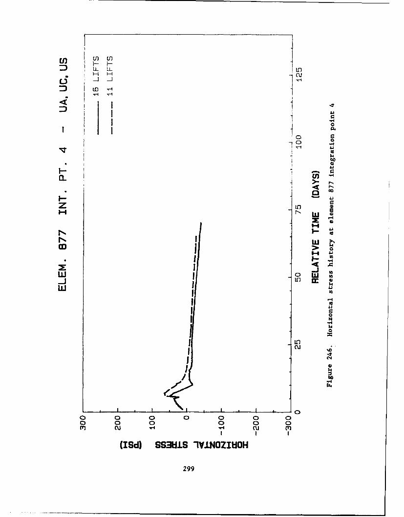
U] ) (U)C., i-
LL LL in
I I 0
jO 0
CL U)
C3 00
* I4J
Hw
0 W
1 >0
0
I-
(Id S IS -WLNZIO
299J
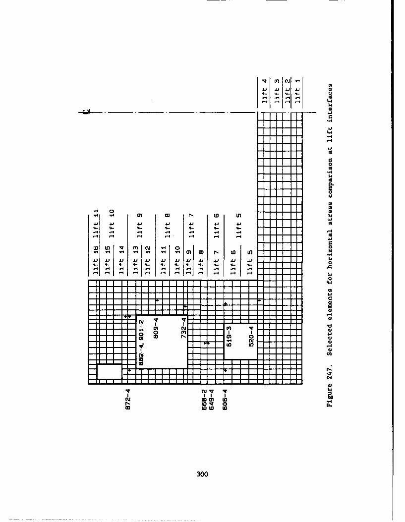
qqm cuH-
41 41 41 41 4)4-. 4- q-. %- 0
.44
$4
"44
$4-
0u
cn m rý ID I41 4141 -W4J F
wO 0 va)c
V1 41 V 41 -W v 41 4 41W.- W.6- W- W '4- 4-4- 06'r4 r4 r4 'M -4 'M W4 1-M
.4.r4 r-4 r-4 r4 P4 r-4 r" r4 r-4 I0 r-
0
644
w ch 0
4)
cu*
El 1. 1 1..
300
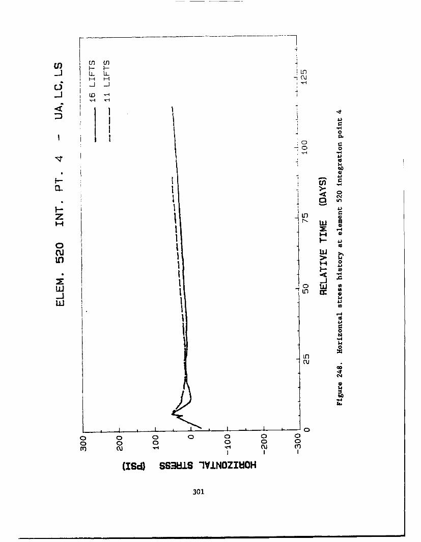
cnn U) cl
Lj~Cu
Lc
Ci ;~Ila.
to0
.~-i 54
:E2 II I I
cu 0
4l >
0
0 U J
Ii 0
r4-
o0Cu w
44
00
0 0 0
301

U3l
14
4 01
LOO
040
C:)
-4-i
CD I
14
0
Cu
1 4)
;34
o 0 0 0 0 0o 0 0 0 0
I ~I
302
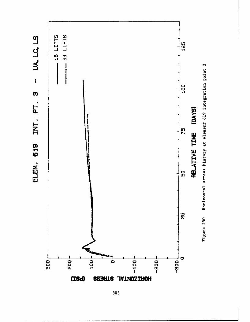
cnn Ell-I-- F-I
"*4
141
LOO
* r 0
1- 41
$4.0
0 1 I$I4I RU '4
2-4
"-4
w.
000 0 a
303
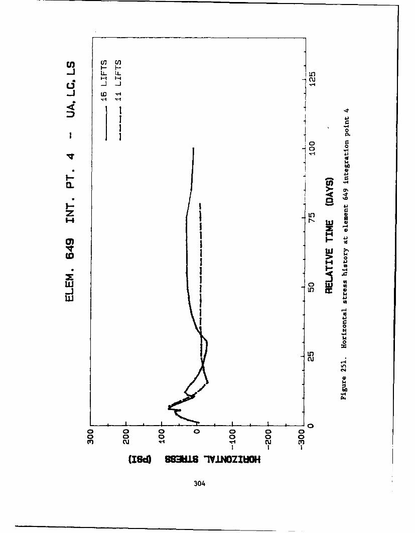
U) C)f
LL LL LO~cu
cs1
,0 0
-401
bo
"4-
* 0%o
> 0
0)13J
CD >0
Livi'-410$4-
II
304
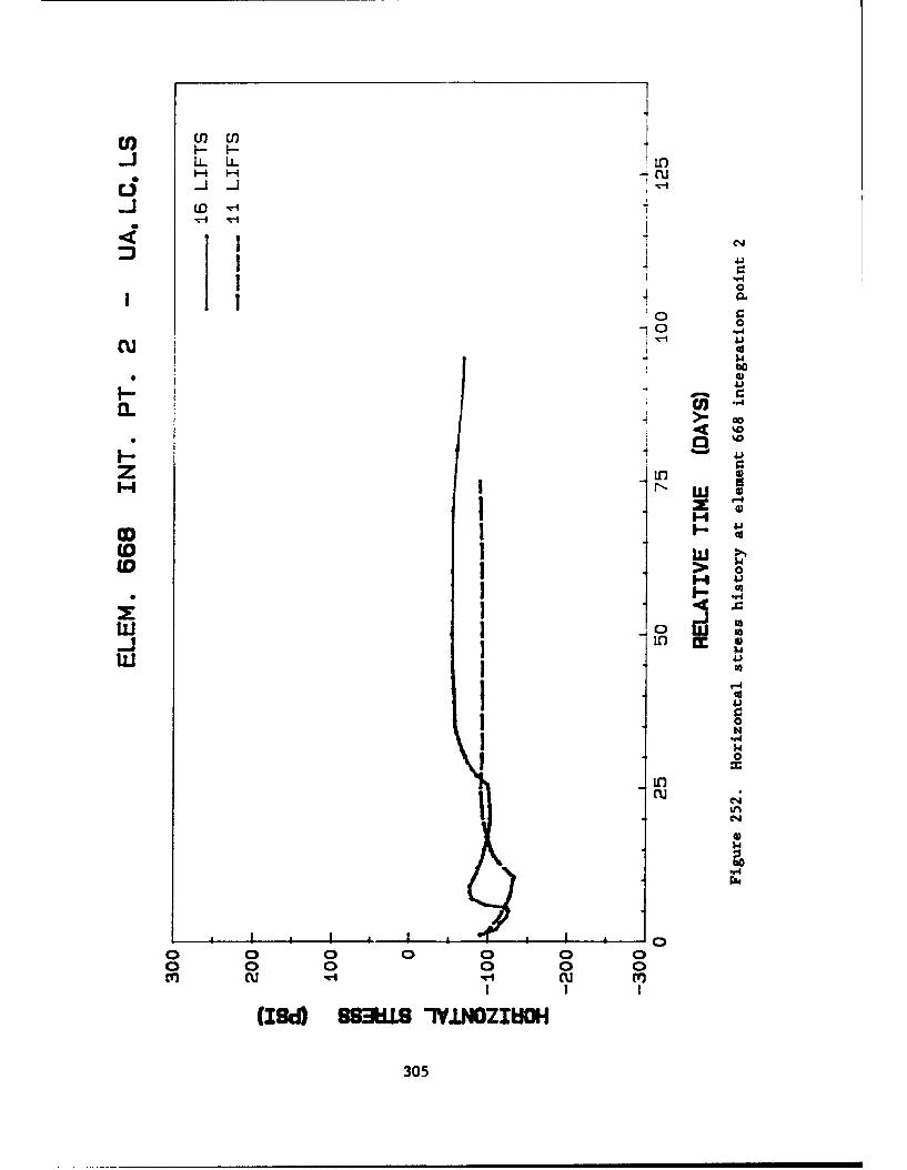
cn uL LL Ur)
LO4
I1 0
cu CbC
%0I-1
14II
I41
I U)
'-4I0C4
0
rtA
o 0 00 0 0o o 0 0 0 0
uclu m
(I~dO SSMILS IY±NOZIUMO
305
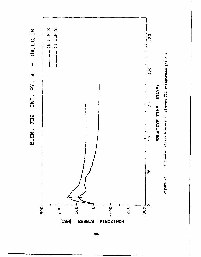
LLL Lfl
III '-4
bo
C4.
H ~4.
I-W
v4.
IIw 0w "w
j r=4
'U
4.1
1 0
1 0I cu m
(I~d 883IS -VINO~ldI
300
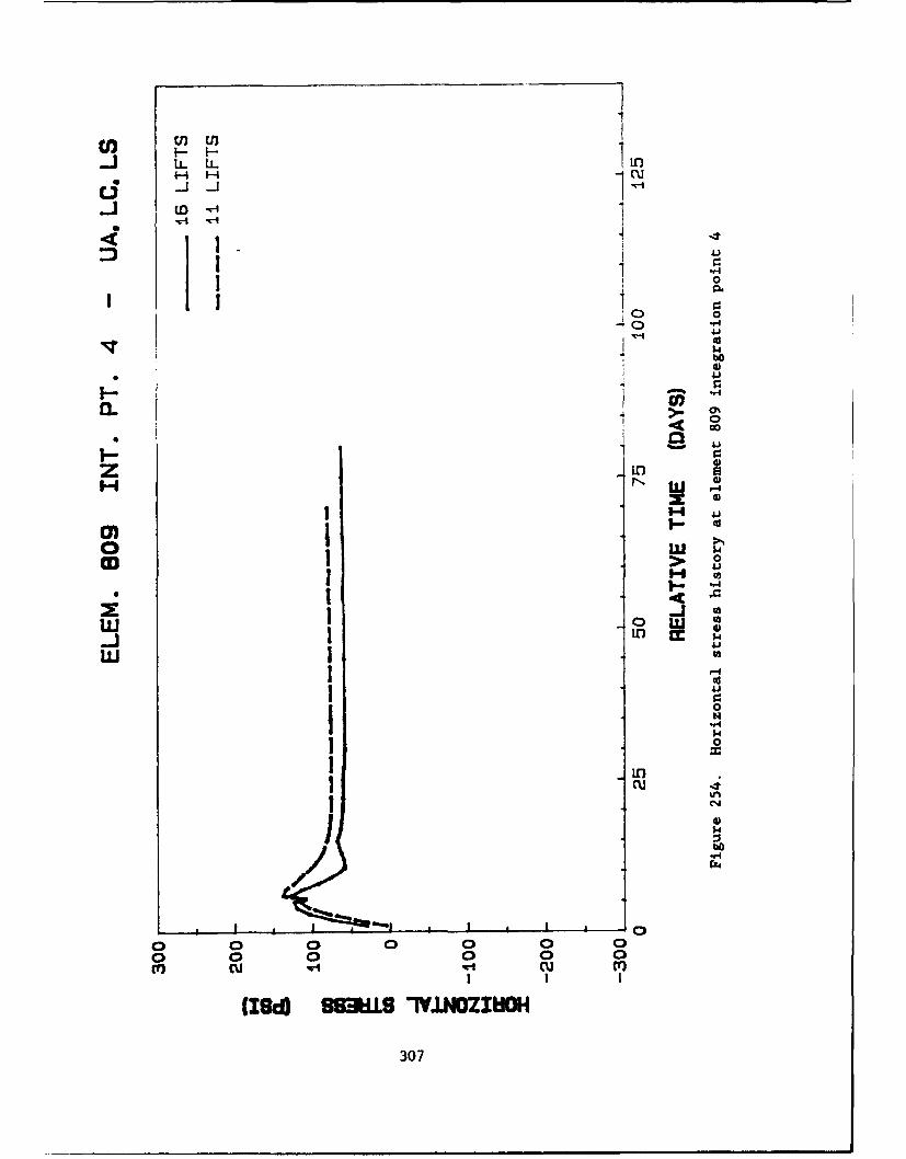
-I-
cid4 $4
.41
1 40IF:Iz
0
U 4 UU ~~o CJ@CI.
14I0100
Inn
C14I0".54
o 0 0 0 0o 0 0 0 0 0
307
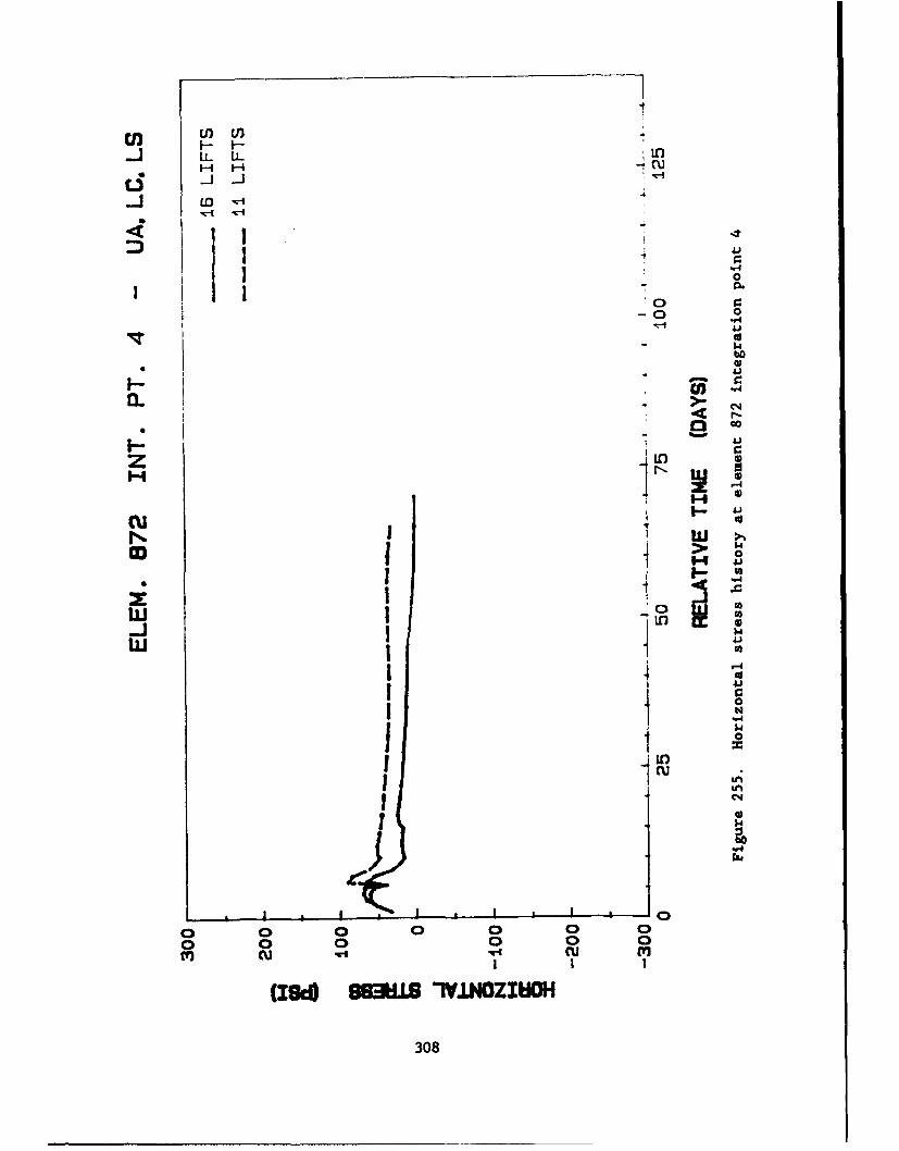
--7U) I-- F
1 41
.4j
IC-4 r,
Ir 4 )
1- '-4
cu cd
I 44
01 ~Ns~
I C."0
o 0 0 0 0 0
(I~d~883"L 1YI.NOZIUOH
308
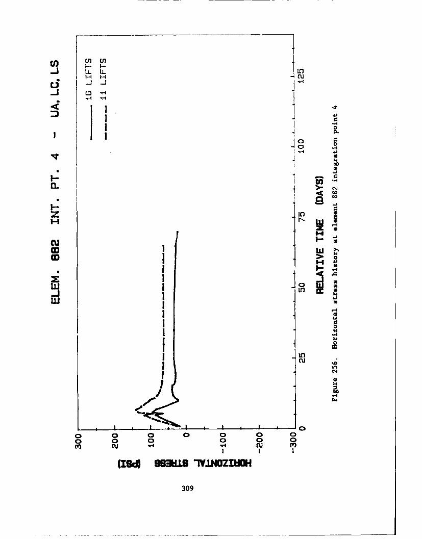
U) U4U)
LL LL
ci ucsD
VtV-4
00
4.)
40 UJ U
1.4
.4J
'A4IA
0
I I I
309
--- - -----
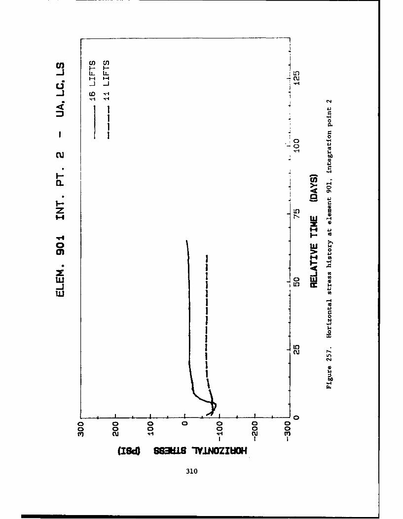
U) u) cfLL L
I "-4
0
I~0~t "-
00
cu bO
z 10
w -4
cn > 0
0)
"4-
4-I
-0-
0 0
310
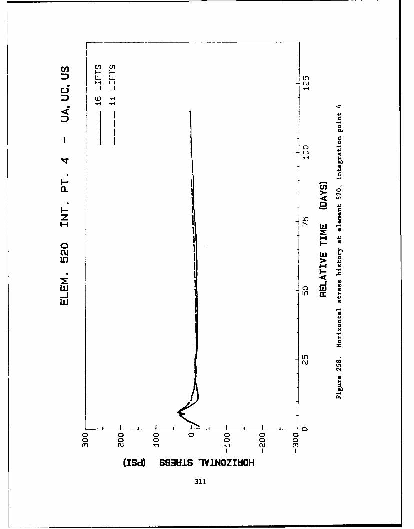
(flWU
LO~O1
r.41 0
4J
14
1- 0
0 m
wIS 4J
o 1 0
in I
* I42:)
$4.
0 0 00 0 00 0m cu '.4
(I~d)SSMUS-IVINZ'EIa
311
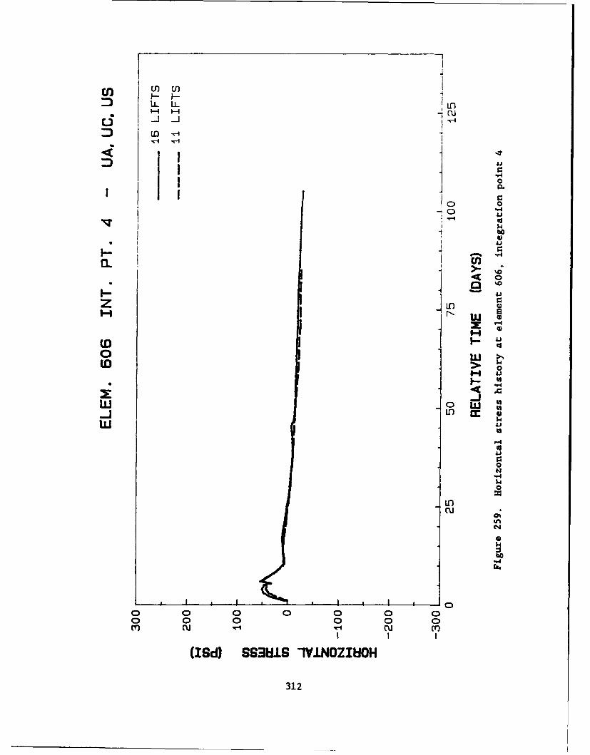
LI L L
10 0-0 "
1 bo
* I 4") )
1u1
0L w t
00
Iu c J
0 0m ru c
(I~d)SUNIS-IVIN'-40
310
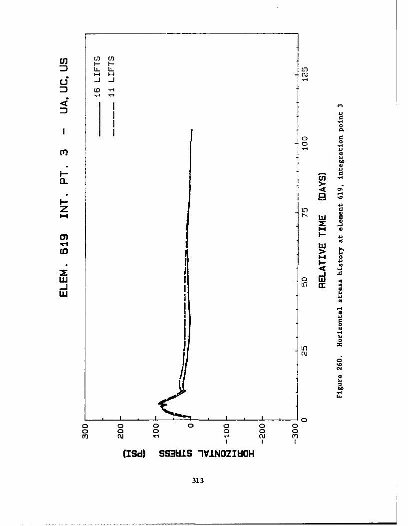
LL LL )- 1-4 1-4 -CU
I 11-D 0
41
be
_ 4.)
CLl* 40%
* 4 1S
0)) 1-
'41*) I-I
U: > $4
I 0
w 0 0 '
~0N
0o 0 0 0 0 0 0o 0 0 0 0 0
cu T Icu mVI I I
(ISd) SS3W.9 1VINOZIEIOH
313
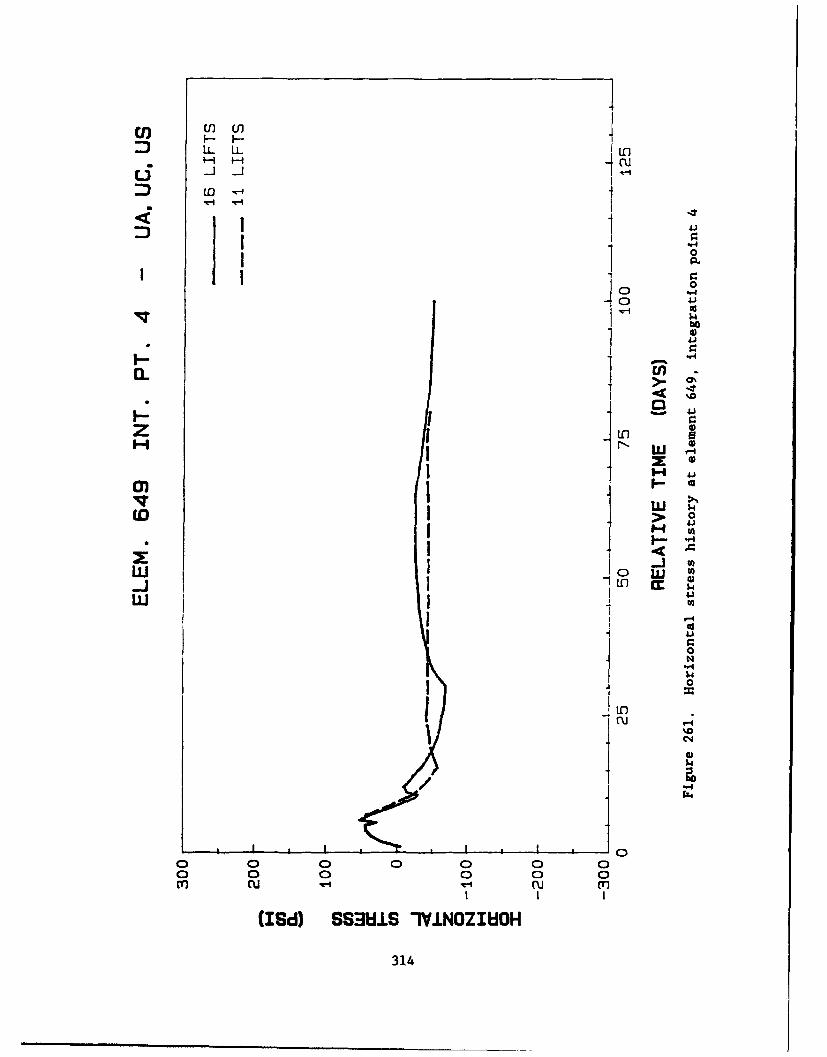
U) F-U0 LLL "I-'
~-' IC'ES~to4
W 0 U 0
w M
0V.4
0
I-, NW LL)I '-I ~m
9-I4
I W )
314i
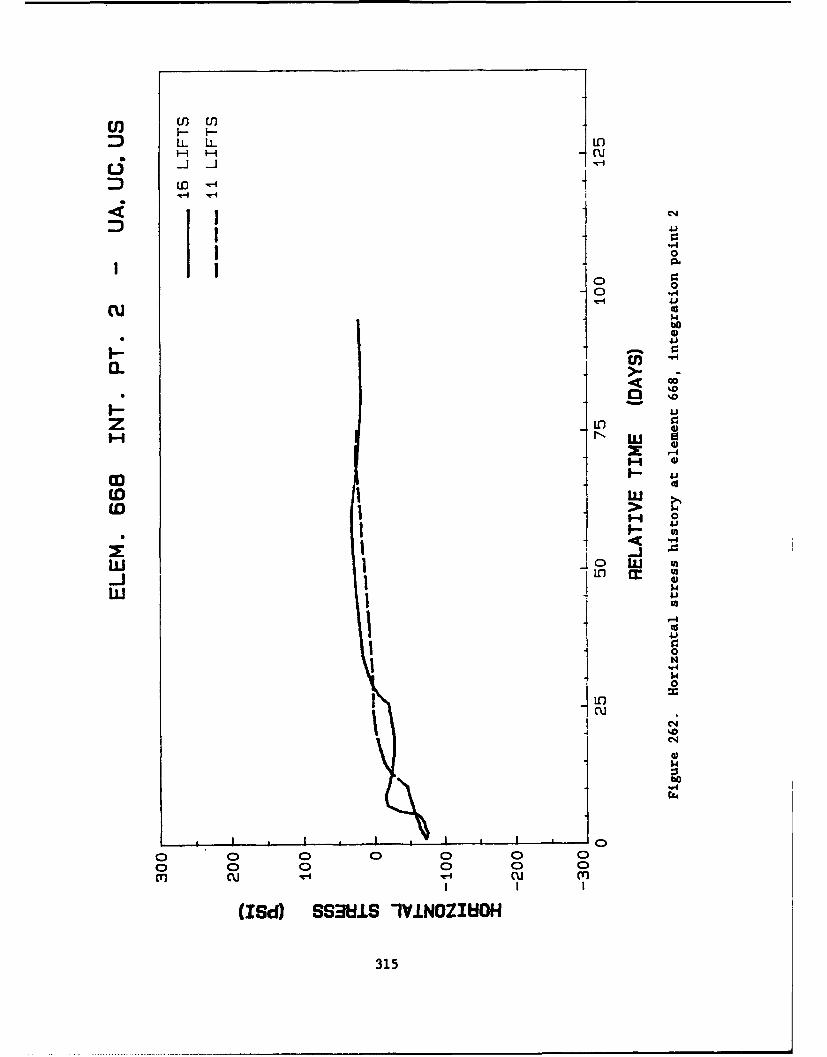
cnc cl) Cl
:3 LL L
cs
1 0"-441
cu CbD
0
4)
t-I
> $4-J I 0
I 0
I
0
1 .4
'.4
0 0 0 0 0 0 000 0 0 0 0
CU c-' CUC)I II
(ISd) SSMI.S IV.LNOZIMOH
315
44
1 ~41
F--
UJ
z U,
cu 4)
Jr 4UJ )
w 0".4
I U)
1 0N
0
cu
0 00
o 0 0 0 0 0m cu cu- '- Cn
I I I
(ISd) SSMUIS 1YINOZIUdOH
316
cn L
1n I--
0 041
< C)
%-w 41)z ILO
041
r14I Id
%0
/ It
I I(1d S8SI INZ~dl
317\
U)' U)-
j0 0
0 "-1
bo
1%- I in>.0
w V
0
1 0
2: -jw Iu
.44
1 0 0 0
cu cu m
(ISd) SS-W.S 1YINOZIUOH
318
0~ HL
tLO
0 00 04
1.4bo
I-.
F- 41z r.
0z43a-I)
Cu A
CDdI 0
I '.4
0 0
II
319~
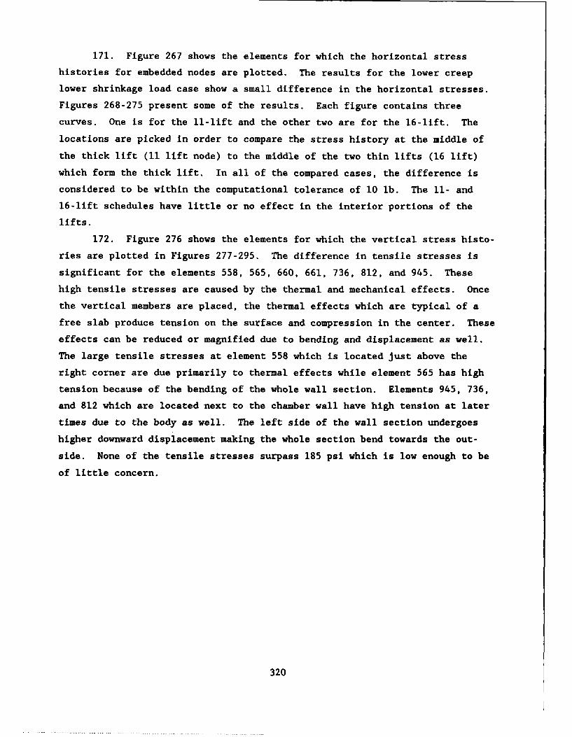
171. Figure 267 shows the elements for which the horizontal stress
histories for embedded nodes are plotted. The results for the lower creep
lower shrinkage load case show a small difference in the horizontal stresses.
Figures 268-275 present some of the results. Each figure contains three
curves. One is for the 11-lift and the other two are for the 16-lift. The
locations are picked in order to compare the stress history at the middle of
the thick lift (11 lift node) to the middle of the two thin lifts (16 lift)
which form the thick lift. In all of the compared cases, the difference is
considered to be within the computational tolerance of 10 lb. The 11- and
16-lift schedules have little or no effect in the interior portions of the
lifts.
172. Figure 276 shows the elements for which the vertical stress histo-
ries are plotted in Figures 277-295. The difference in tensile stresses is
significant for the elements 558, 565, 660, 661, 736, 812, and 945. These
high tensile stresses are caused by the thermal and mechanical effects. Once
the vertical members are placed, the thermal effects which are typical of a
free slab produce tension on the surface and compression in the center. These
effects can be reduced or magnified due to bending and displacement as well.
The large tensile stresses at element 558 which is located just above the
right corner are due primarily to thermal effects while element 565 has high
tension because of the bending of the whole wall section. Elements 945, 736,
and 812 which are located next to the chamber wall have high tension at later
times due to the body as well. The left side of the wall section undergoes
higher downward displacement making the whole section bend towards the out-
side. None of the tensile stresses surpass 185 psi which is low enough to be
of little concern.
320
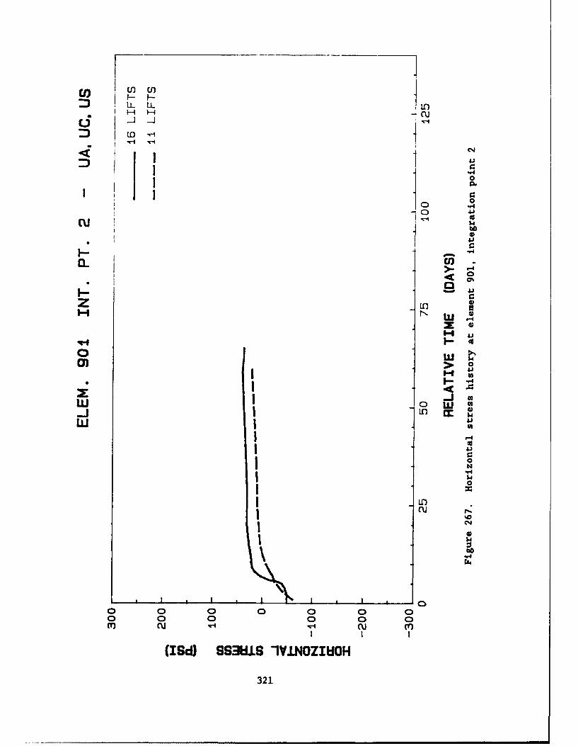
iwU3
Lo
I-c uc
I j j
> 0
I j44
ILl
.14
I- t
IIwId SSa IL! 02IUO
-j j 321
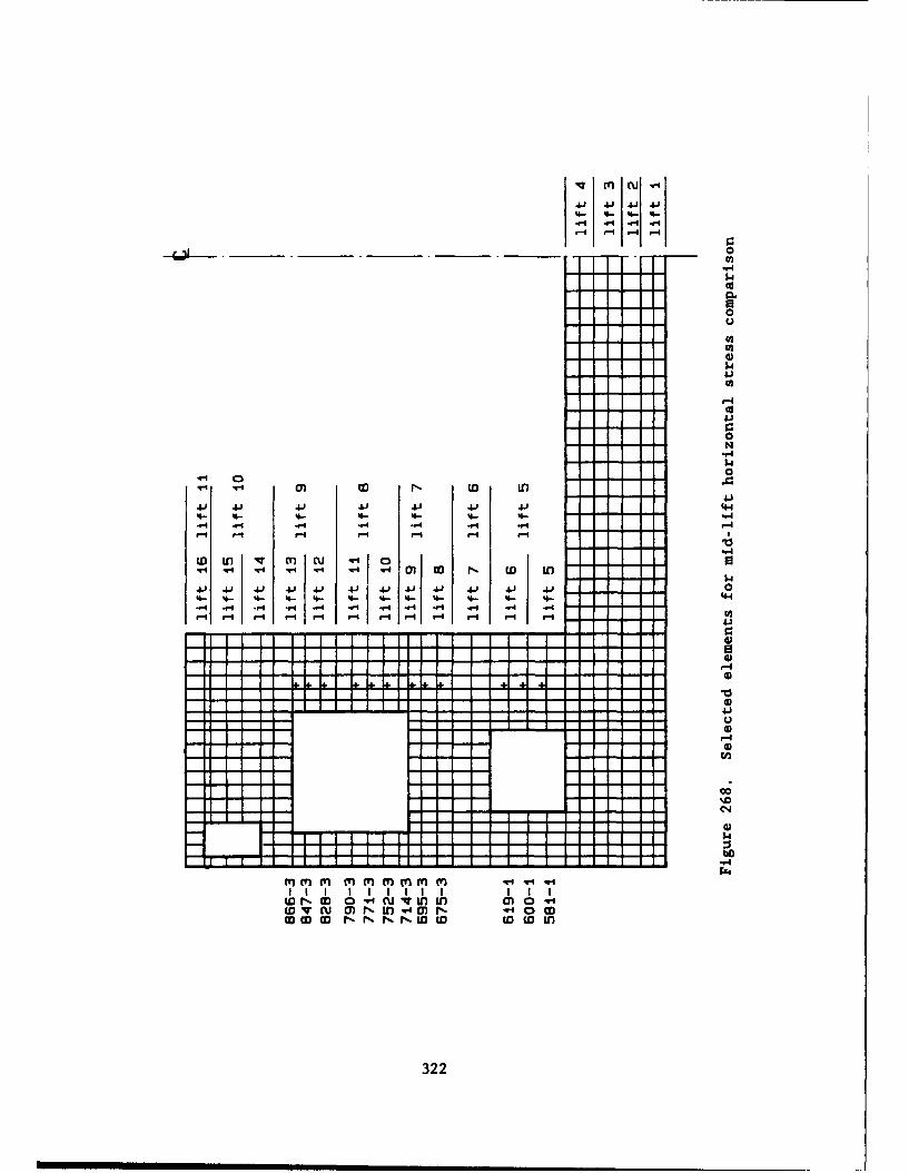
qq m cuJ.
43 44V343)
'0
0
cn LO
"43
-.4
.4 0
"4.
'-0- '4M V0 If) 0- a)- '0to4 IV .4 a) N .f 4 .4 N 4 0
.4. a4 OD. r-l40 NJ N. N CD(D In)
3223
o to
0 CC)
1i-i I
LI Id I
u, En EnIL LL LL
"-(lED I O
1 1 0
0
"4J
Er 011 N LI
II 0I-, 0
1-U4
4)14.
"IA
P4.
0 00 0
In cu cuI In
(I~d) SSMI IVINZI80
323%
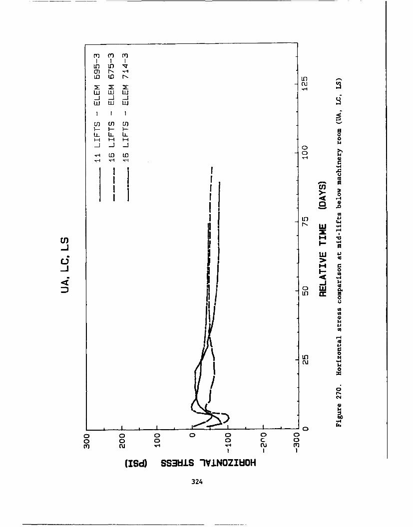
MT ri-i
U) In U
u O LO 0
in ininF- I- F-
l0"LU0 w C
Ln M RIi I0
1 ~4.NW 0
ICI4cn IIII-., *
IJ IIId S31 IVIN 'Ii0
13 1'324
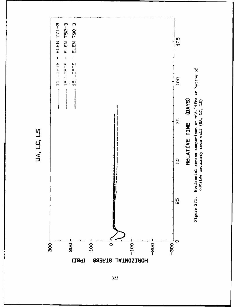
'm mI I I
" CU OLD
Lu Lu Lu
r- - In
LL LL LL 44
0041i
LO LO o4
"DqU
4-
0i 44 14 Iw
LO 1:1
'44)
Cz4
0o 0 0 0 0 0 0
o 0 00 0 0
(ISd) SS3W.1S IVINOZI80OH
325
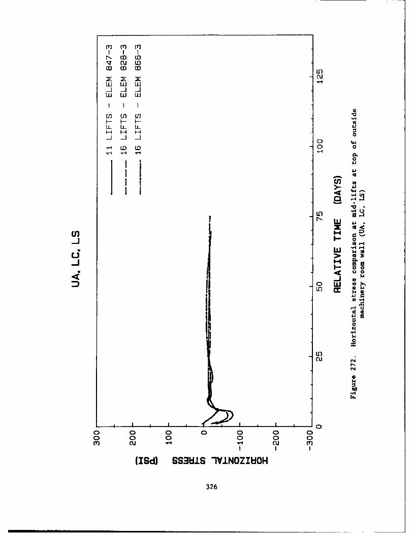
I I I
NW IW
Ui Lii Lu
0 44
~ 0
~~-i in in0~~>- 41~-
I L L i
> ccn )
6'a-o o
$4
cid- 00
4 00
0 0 0 UJ 0
(U cu m
3264
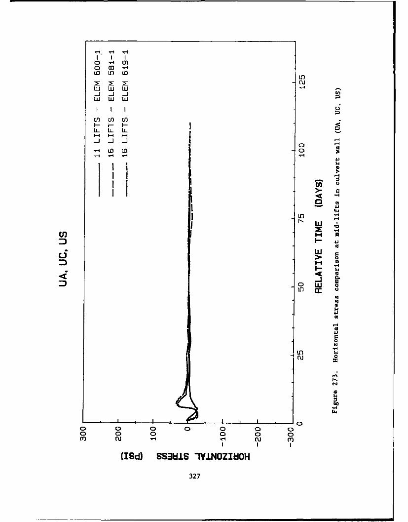
(LD U" 0I
~ Cuw w w-i I I -
I-i -H
~J ~J~4-4 on "vi (00 o C
> o
Ii- 1g.2o0
-4
(~) >0
""40cu 0
00
02
$4-02
"-4
C)u
(I~d)SSMIS-IV.LO"IWI
327).
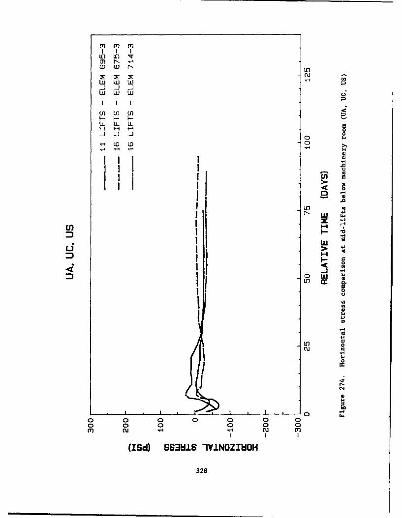
(T) (T) (7I I I
UnL) -4m N -- 4(D EDN LO
LI LI LI C
LI Ij IL
u) U) cn
LL LL IL
II I-A I-q 0
LO1 LO( 0
34J
0 -
IN Lu 4144
C3 co
W $
0
1.4
U) 0
cu cu 4II(I~d) SSAUS'IYINZIM4
328
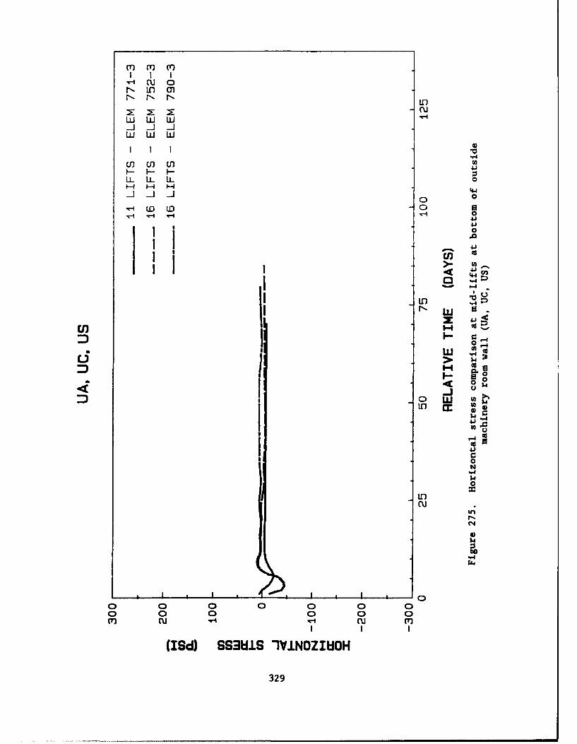
.~' cu 0r- Lfl 0nr- r- r- 10
I I I
U) inu) W)
Li. LL LL 0'4-1
0 0
-1LOWL 0 0
41)I ~41I .0
41)
ii~E I - nI 2 FA
'~~4
0I W 'd> 4
u $4
$4-
-41
2.4
0InN
LOO
.9.4
124
0o 0 0 0 0 0 0
o 0 0) 0 0 0cicu Cli (7
(ISd) SS3W.S 1IJ.NOZIWOH
329
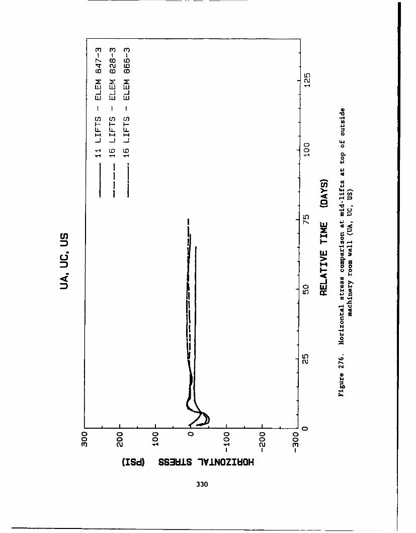
(r)m mI I I
r- W LOc u wo
L LU I IW
LL LL LLU:
ILO LO I
0
~~"4 C-4nr4
I JJ
w 4jUd
x'-4
(3 o
j _'
r-4
"-4
;24
00
o 0 0 0 0 0o 0 0 0 0 0mcu '~ ~cu
I II
(ISd) SS3W.S 1VJ.NOZI~dOH
330
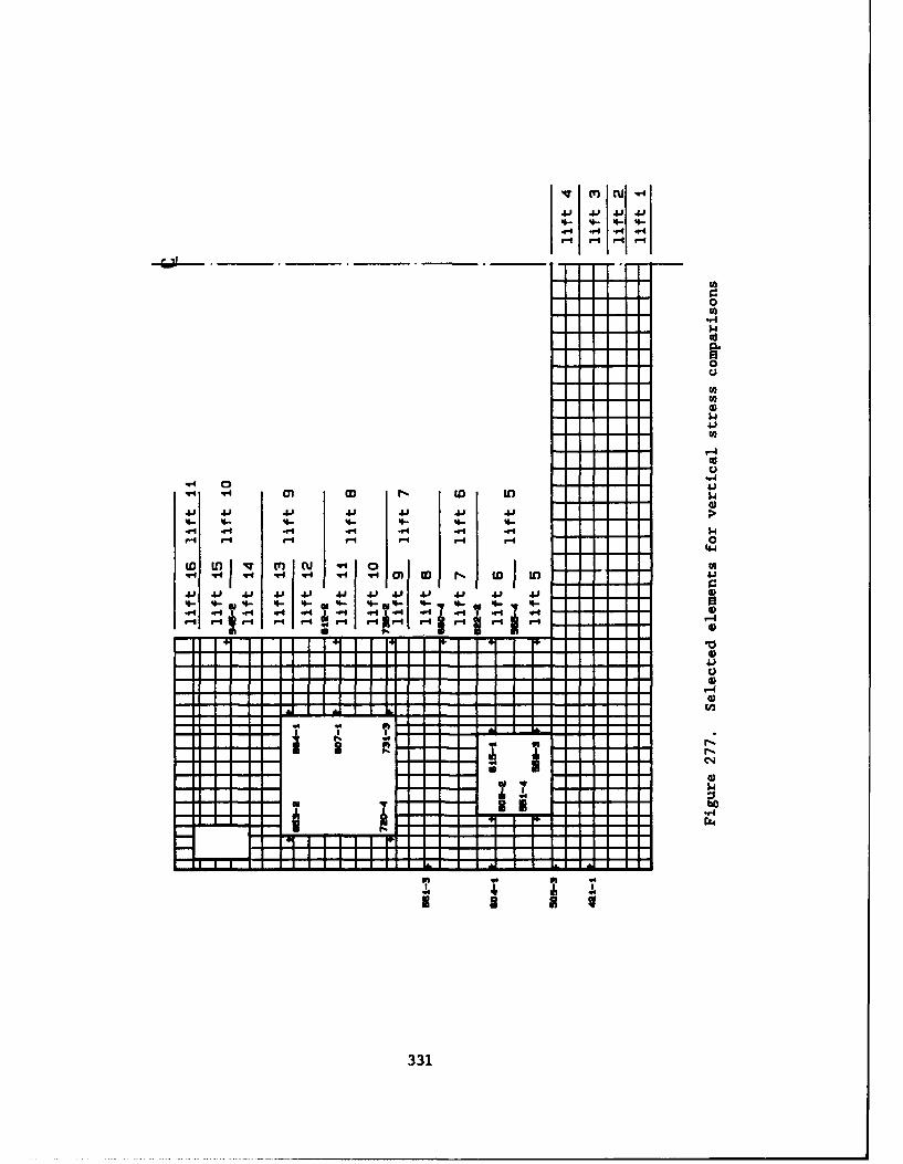
IVI m 1u -4
0
.94
41 >
.4 0 _
94I .4I r-4 r_ .4D .
r 4
CD Uq
3313
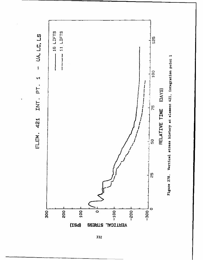
InH 1-.4
.bO
0J
0 H4I;1
1-1
IL aoj4J
Lii / 0
LJ / W)Lo)
(IO$4
1jcul
I I I
(ISd) SS3HIS 1Y31.LEMA
332
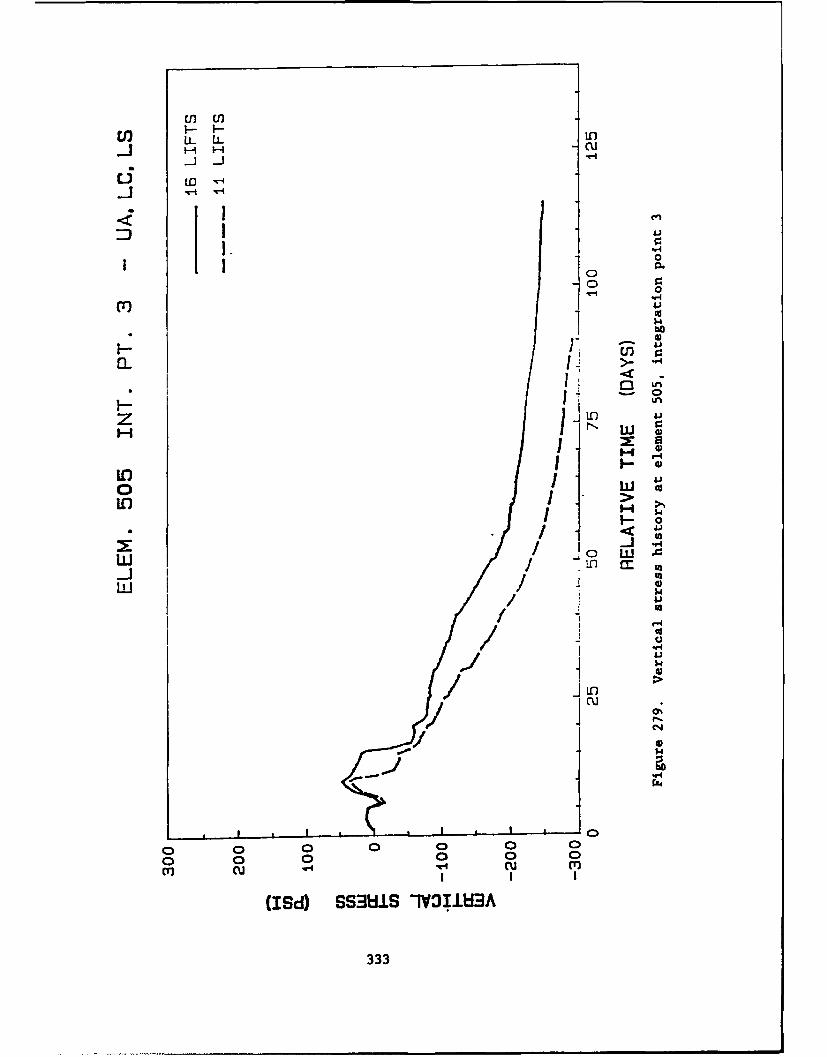
cn EnH
LL~b LL
(T))
4 bO
4)
LL -W
H Il
I a)
In I n cc
In
0-4
-0/ 0 C)cn cu W4.c
(I~d) SMIS -3IlU3
333a
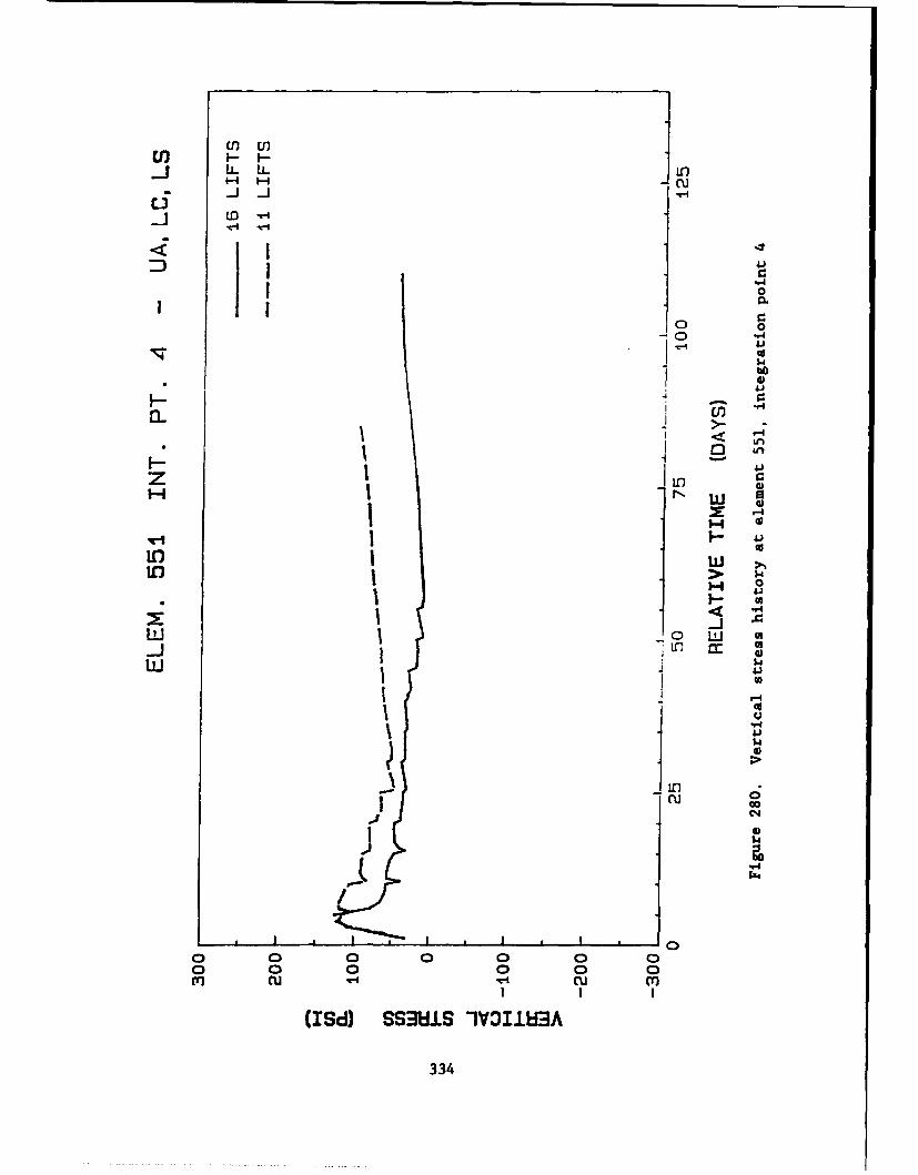
U) I--
LiL
0 00 o4
* 6)
LL n- -1
*L 0
0
Wn 0
U) 1)
I 0
I 0
3344
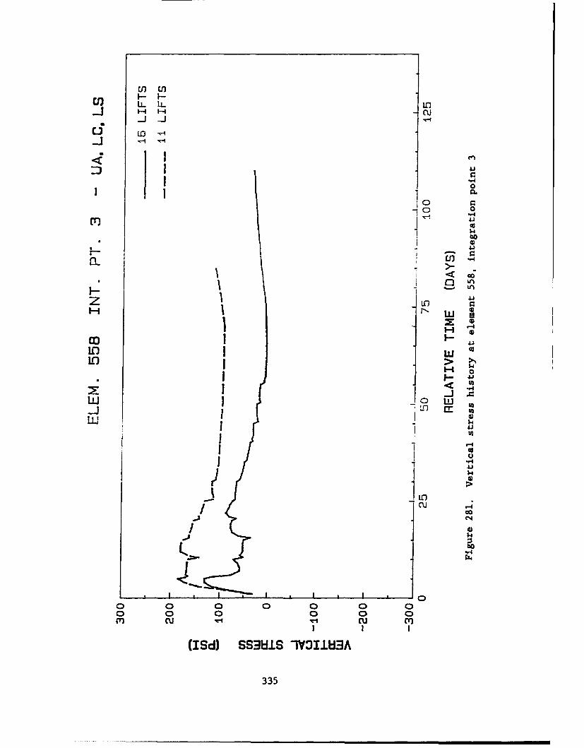
U, LO
c-;n
00
@bO2.
o-WI - Ul
I-I N <
LF)n
44)ww aQa)r 41
11 w c
LO > t.1
1 U
'-oI0
4)
bO
00 o 0 0rncu cu c
I ~II
(ISd) SS3W.S -W31183A
335
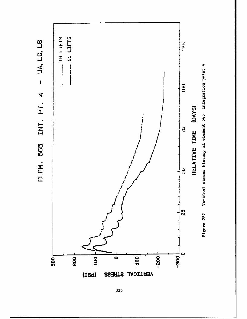
U, ILL U.
dc* 4)
LOO
41I
ED -L
II
/ r-40
to I $4J
LLO cI )
*1 / 0
".4
In 0ucu
(Id)SSH SIVIrG336n
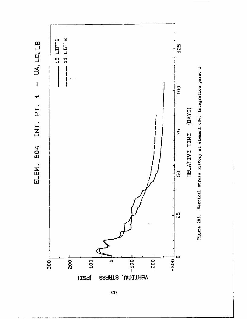
cnc
~ 1-4
II 4.)10 cod
Il40~ 1 4.
14
U)
C3
LOL
1~4)0
ED 4:02
/<
/ Ln
4)
00
o 0 00 0 0o 0 00 0 0CU cu cu In
II I
(ISd) SSMI1S 1Y21183A
337
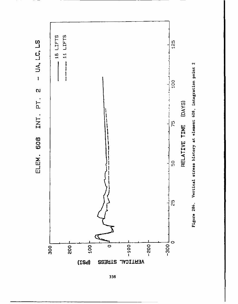
LO~
0
0 r1-0 0
* s-I
* 01cu _ o
1-4 0
IL 0)
m ~4*0 1 w
LD c
I- 4 0-
4.A
w LI dU
I 0 1W
'I
-~ 0
Z44
0
o 0 00 0 0 0o 0 00 0 0
(ISd) SSMUIS lV3118:3A
338
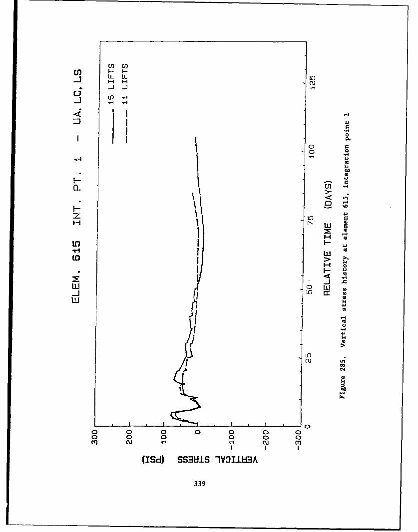
C,,dJ~ au
ob
14* 41
I L < U ,
*L I0 0 )
ww
U) 1 '-41
LLW
CD N
*-rd
W 0 -
0 0t 0 02(0uJ n 1u .1..
(I~d) SS381 -lV3l~f3
339W
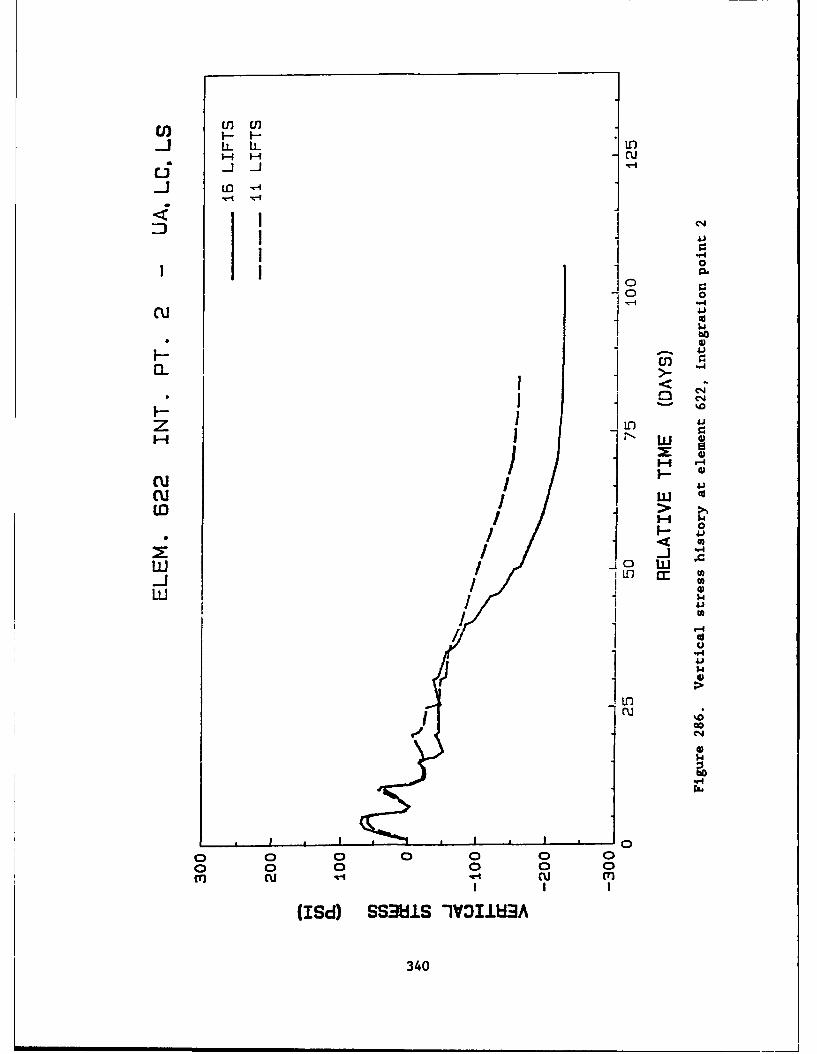
C, I--LL LL-"
LiLLD14
-. 0
0
cu 4* C)
* ~41I->-
z 41
Cu 4
~~0
'o IL A'
I ~4-
Cuu
i14
3404
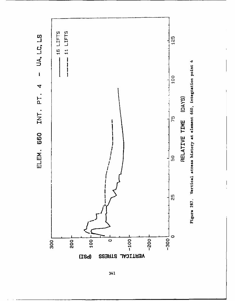
U) LO'
(D~
Ia0
.11
n "4
I- -% JJ
Do
C)LUA
COd
1.4
I El
3414
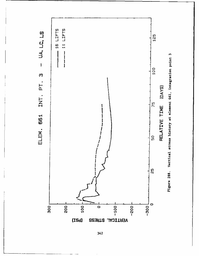
LLLL L
000 0ob
0
CD Iw 4J0
1-404)
-LJ I)
ci
1 U1
"(4
o0 0 0 0 0 0
(I7d CUMI CU C')3
342
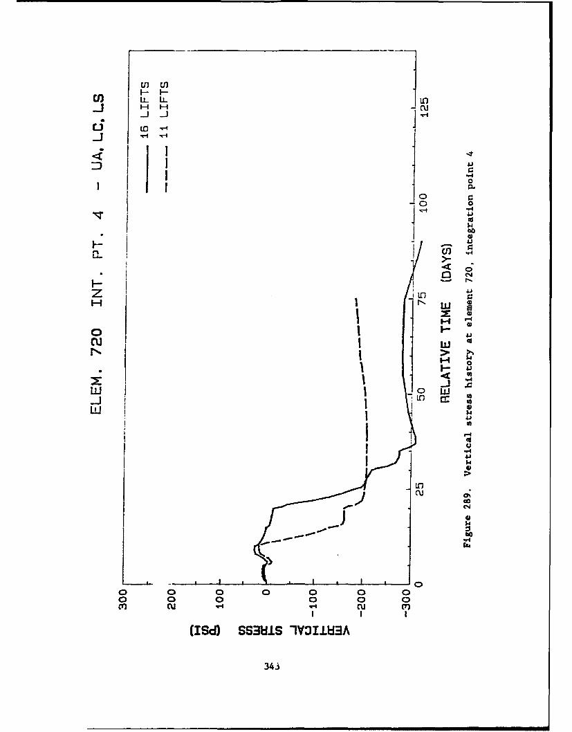
U, U)
bo
<0
I I -
0 W
I~4.)
U')'
0 0
0l 0 00
3434
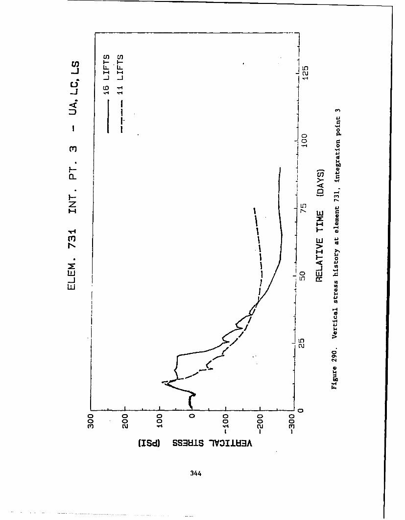
I-'--LL LL -cx
Ai-
1 0
j 0
-. 0 0
j~-l 0
(TJI$
-L '4
I- I, c
0 0.0 0 0 0
m cu clj r
3444
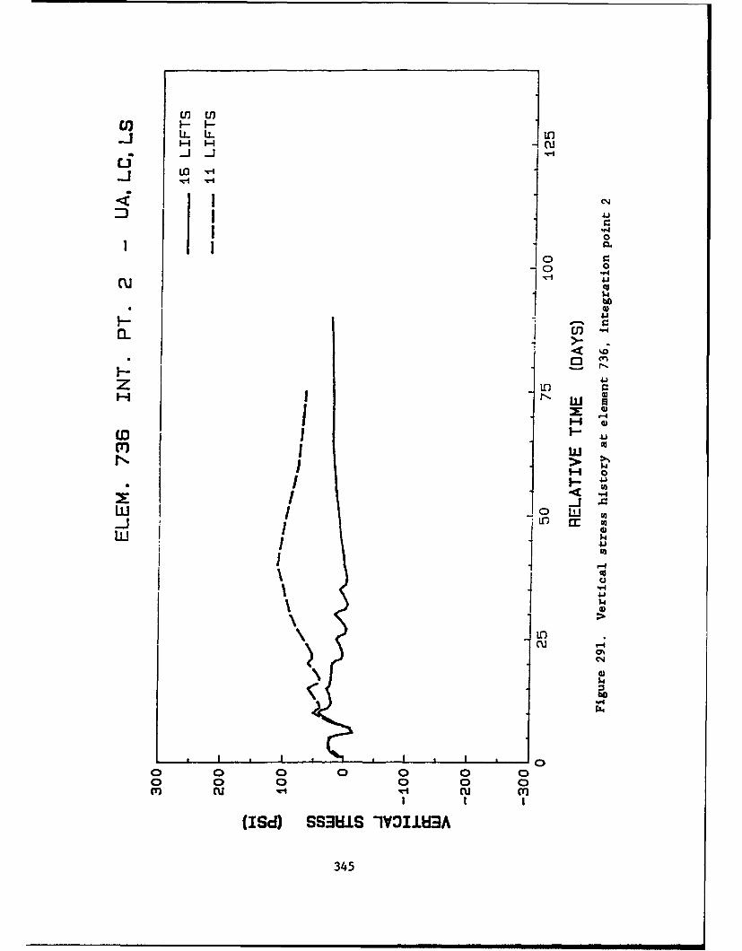
tn EL
0I 00
0 0
cu K L
-- r"
H LL EZ U)
M ~w c
> wý14
HoI<
1 141$4
)4C~4
).r
o o 0 00 0 0o o0 0 0 0m cu ' cu (n
(ISd) SSAWS V~3IfIH3A
345
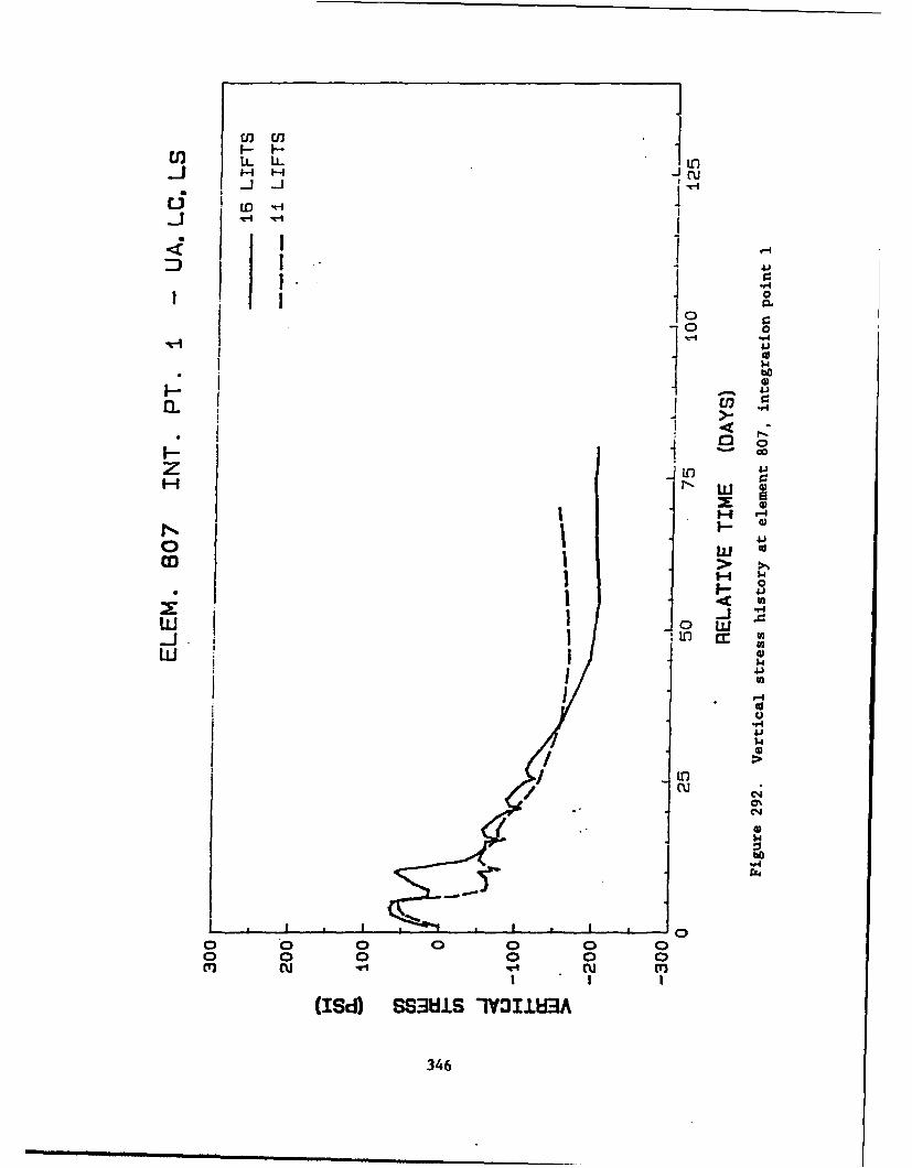
En nU) LL LLL
CJ Iwu
* 0
H 1 0
Z 'a
co > ,.
I $4
1~02
LOIcu 'a
2.4
/$I Lr.)/ PN
C)%
00 0 0 0 0 0
346
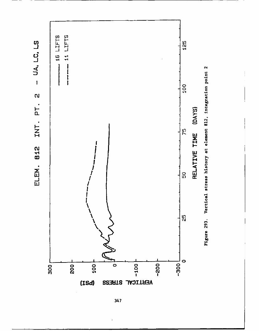
U) ItoL W
C.C3
1~".4
I bo
< C ;,
F- OuD .
cIii
wo >j0
w n a:
w 1 1
C4.
00
II
3474
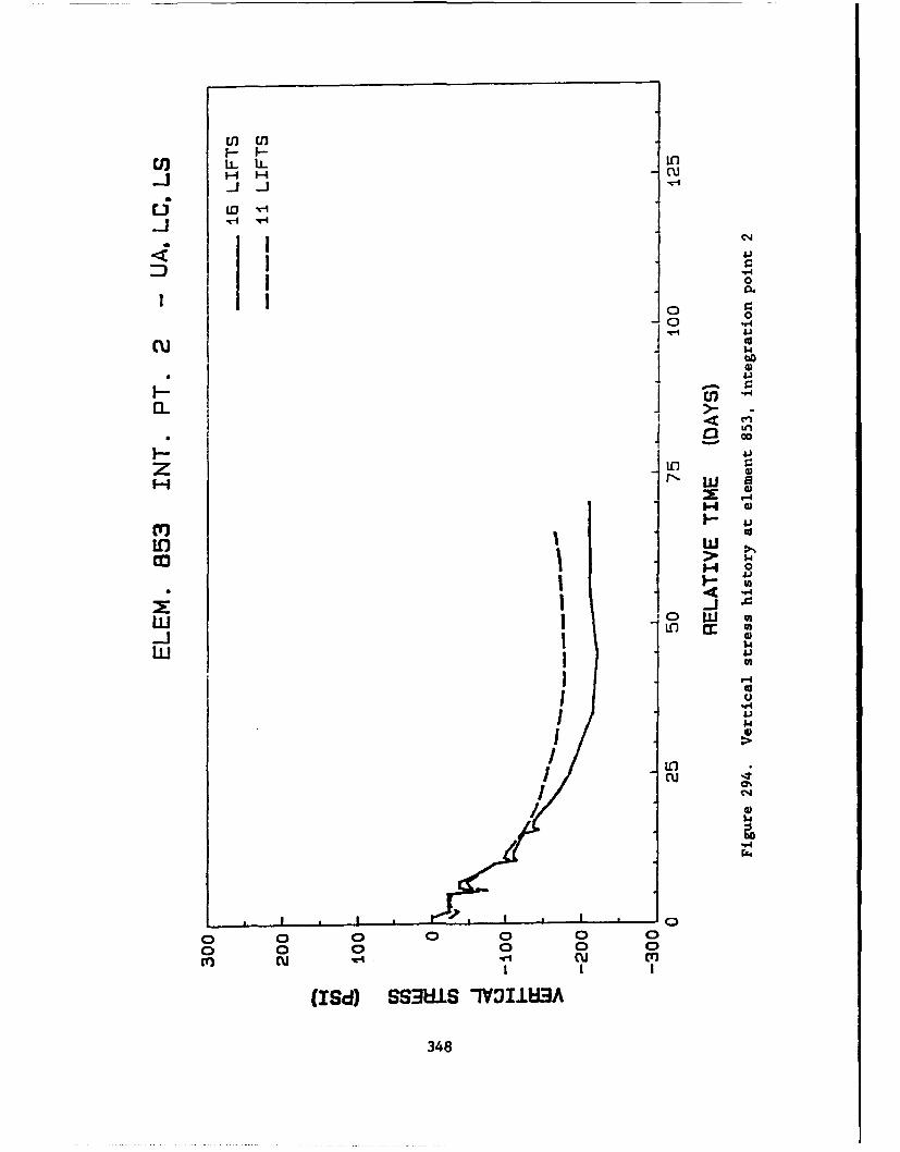
U) -L
C4.
I 0
0 01cu I o.
LOO
v44)
cn Cn> 34
.41iFA
1-4 2
C:) W A
U)U
1 ~4."5 40
1 2 1 0a0 0 0 0 00wu cu 'c
-Jd SEU YIG
3484
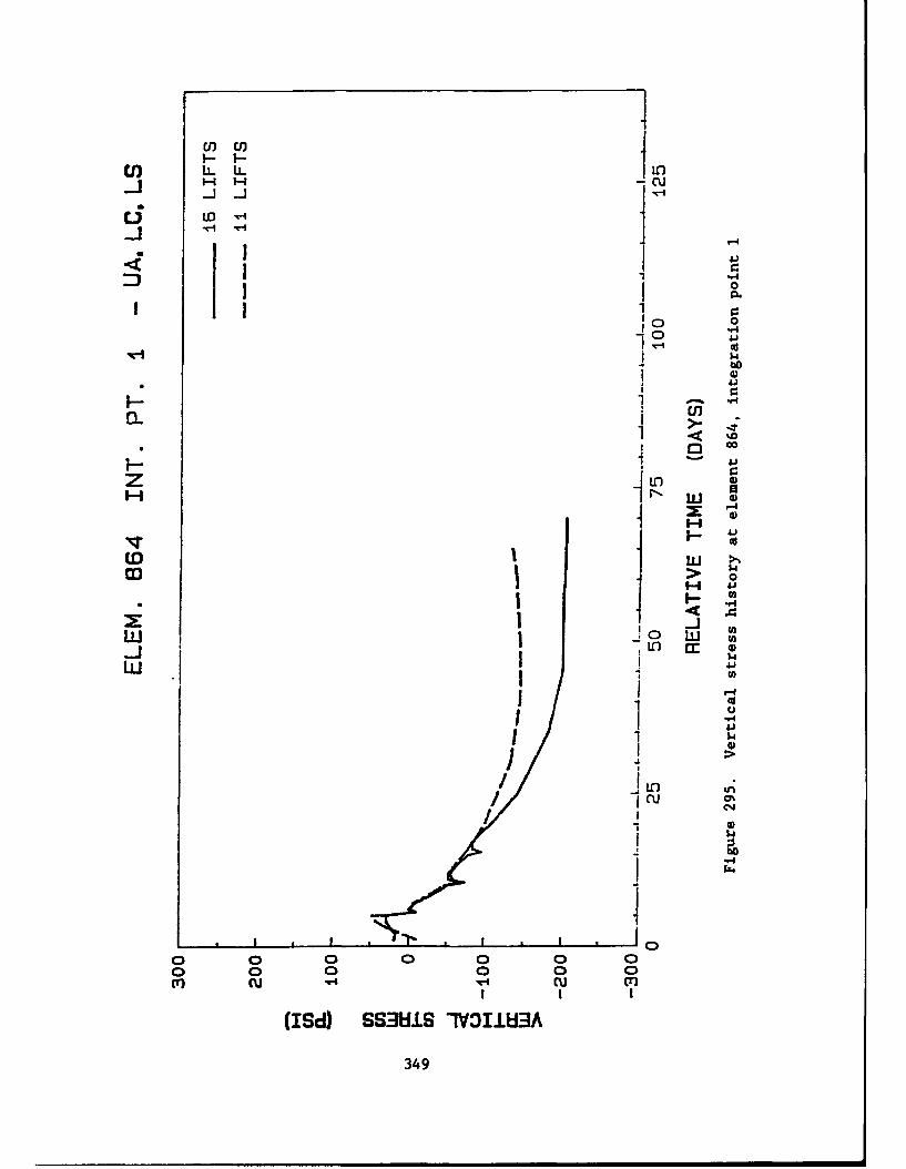
Es L
C) 0
1.4
cn
IL >-
CD 0
co o
I 04
I 0
o00 0 0 0CT) -W4 cu I
(ISd) SS3MLS 1V3I113A
349
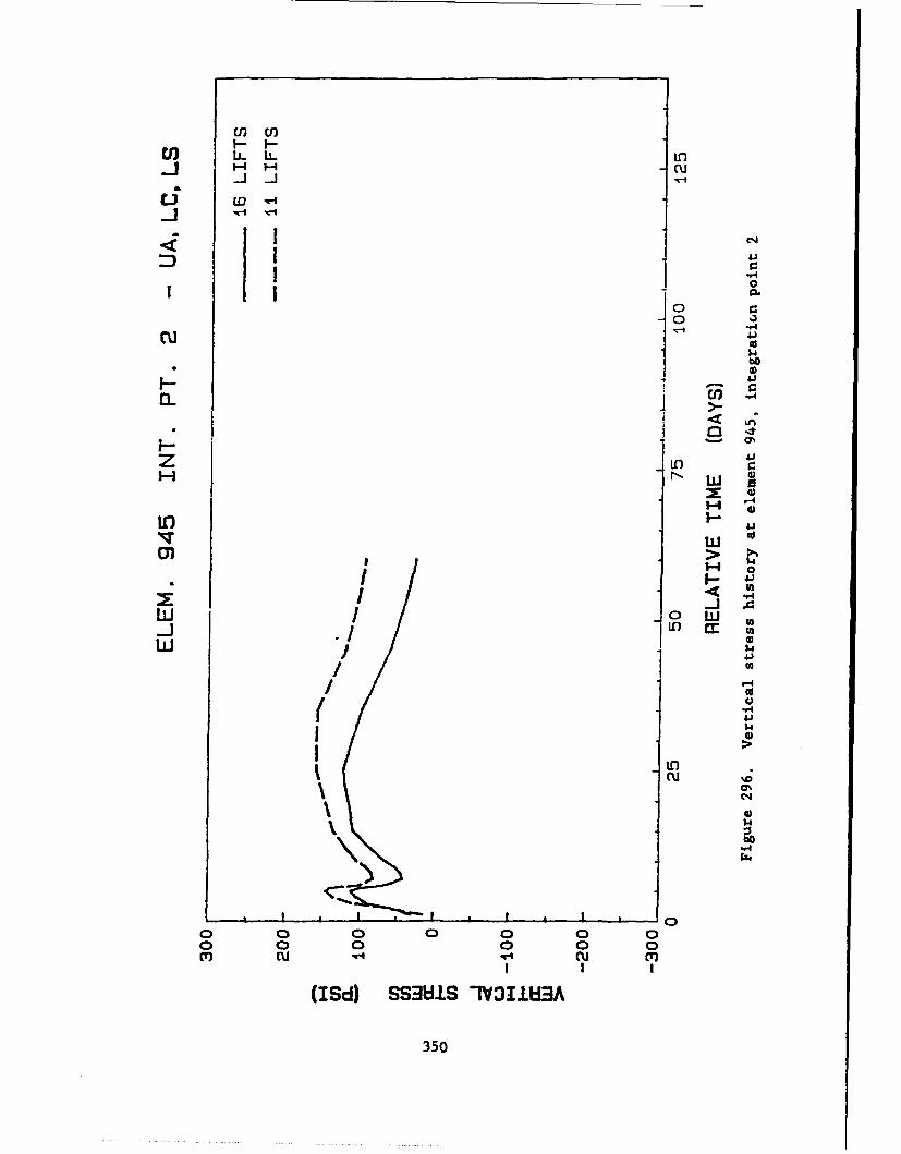
U) (I LL LLL
cu
C.,4
0
C~41
04
Z 1L0
LU
'-0
_jI .1 1( $4
cu
.44
0
(Ird SSMI '4 CU CT
350
PART XII: OVERVIEW, INTERPRETATION, AND CONCLUSIONS FOR MONOLITH AL-3
Introduction
173. The significant findings from the previously discussed results
will be restated. In addition, an assessment as to the meaning of these
results and any pertinent conclusions will be discussed.
Overview and Significance of the Results
174. First, the modelling procedure was explored both with respect to
the heat transfer and stress analyses. (The material model was supplied
through WES.) It was concluded that Equation 2 (limiting element size) could
be violated in the horizontal direction in the slab and soil since the heat
tended to flow perpendicular to that direction. In addition, the soil depth
could be cut from 20 ft to 10 ft and still produce nearly identical results.
This reduces the required number of elements by 20 percent.
175. The use of gap or interface elements was essential for the soil-
concrete interface if the results at this location are needed. If the results
near that interface or early time results are not required, interface elements
would not be needed.
176. The use of air elements and multipoint constraints (MPC) should be
analyzed further. The correct initial properties for the air elements are
essential to produce reasonable results. The initial temperature for the eir
elements can greatly affect the rise or lowering of the surface temperature in
the void. The MPC's are also of some concern, and more detailed study of the
load transfer at the end nodes should be explored to ensure that correct
results are being obtained at the upper corners of the openings.
177. The lower bound creep and shrinkage load case consistently pro-
duced the highest tensile stresses. The maximum tensile stress seen in the
monolith AL-3 was approximately 180-200 psi for vertical stresses on the cham-
ber face which is due to both thermal and mechanical effects. The other crit-
ical location is in the slab near the center of the chamber where the stresses
reach approximately 250 psi just prior to placing the first lift in the wall
section. Once the placement of the wall begins, the tensile stresses begin to
reduce due to the bending of the slab. (Eventually, this location has a
351
stress of approximately 250 psi in compression.) Also, the top of the slab
shows a stress of approximately 450 psi which is very large and undoubtedly
would cause cracking, but this appears to be primarily due to the bending of
the slab and could be controlled by placing tensile reinforcement in the top-
center of the chamber floor. This high stress is identical for both the
11-lift and 16-lift schedules and is, therefore, independent of the construc-
tion plan.
178. The most significant result is that the 11-lift and 16-lift con-
struction procndure produced nearly identical stresses and strains at most
locations. The maximum deviation in stress between the two models occurred at
the void floor surface and was 130 psi with the maximum stress being 180 psi
at this location. A stress of 180 psi is well below what would be considered
a critical tensile stress. The next worst case is a difference of 70 psi with
a maximum of 150 psi for a location at the lift interface. It can be con-
cluded that the 11-lift model produces no significant increase in the tensile
stresses compared with the 16-lift construction. Therefore, the 11-lift con-
struction should be used and could save a minimum of $700,000 as demonstrated
(US Army Corps of Engineers, St. Louis District 1988).
179. A three-dimensional model for a portion of AL-3 was developed.
The intent was to verify the two-dimensional results and provide guidance in
simulating the actual three-dimensional state with a two dimensional model.
Due to the enormous physical disk space and other complications associated
with the program ABAQUS and the three-dimensional material model, the analyses
could not be completed. These problems are being addressed and large scale
three-dimensional analyses of lock and dam monoliths will be possible in the
near future.
352
REFERENCES
American Concrete Institute Committee 207 (Mass Concrete Committee). 1973."Effect of Restraint, Volume Change and Reinforcement on Cracking of MassiveConcrete."
ANATECH Inc. 1987 (Oct). "Development of Two and Three Dimensional Aging andCreep Model for Concrete," US Army Engineer Waterways Experiment Station,Vicksburg, MS.
Fehl, Barry. 1987 (May). "Analytical Prediction of Thermal Stresses in MassConcrete," M.S. Thesis, University of Texas at Austin.
Fintel, Mark, ed. 1974. Handbook of Concrete Engineering. Van Nostrand Rein-hold Co., New York.
Headquarters, US Army Corps of Engineers. 1983 (Sep). "Basic Pile GroupBehavior," Technical Report K-83-1, Case Task Group on Pile Foundation, Wash-ington, DC.
_ 1987. "ABAQUS - Structural and Heat Transfer Finite ElementCode," User's Manual. Providence, RI.
Hibbitt, Karlsson, and Sorenso',A, Inc. 1987. "ABAQUS - Stru.•tural and HeatTransfer Finite Element Code," Theoretical Manual, Providence, RI.
Holman, J. P. 1981. Heat Transfer. Fifth Edition, McGraw-Hill Inc., NewYork.
Hughes, B. P. and Ghunaim, F. 1982. "An Experimental Study of Early ThermalCracking in Reinforced Concrete," Magazine of Concrete Research. Vol. 34,No. 118, pp. 18-24.
Norman, C. D., Bombich, T., and Jones, W. 1987. "Thermal Stress Analysis ofMississippi River Lock and Dam 26(R)," US Army Engineer Waterways ExperimentStation, Vicksburg, MS.
Rawhouser, Clarence. 1945 (Feb). "Cracking and Temperature Control of MassConcrete," Journal of American Concrete Institute, Vol. 16, No. 4, pp 305-346.
Thompson, Obbie. 1987 (Dec). "EXTRACT - FORTRAN Source Code for ExtractingData from ABAQUS Post Files," US Army Corps of Engineers, St. Louis District.
US Army Corps of Engineers, St. Louis District. 1988 (Sep). "Report to LowerMississippi Valley Division on Thermal Stress Analysis on Monoliths AL-3 andAL-5 of the Auxiliary Lock and Dam No. 26 (Replacement)."
353
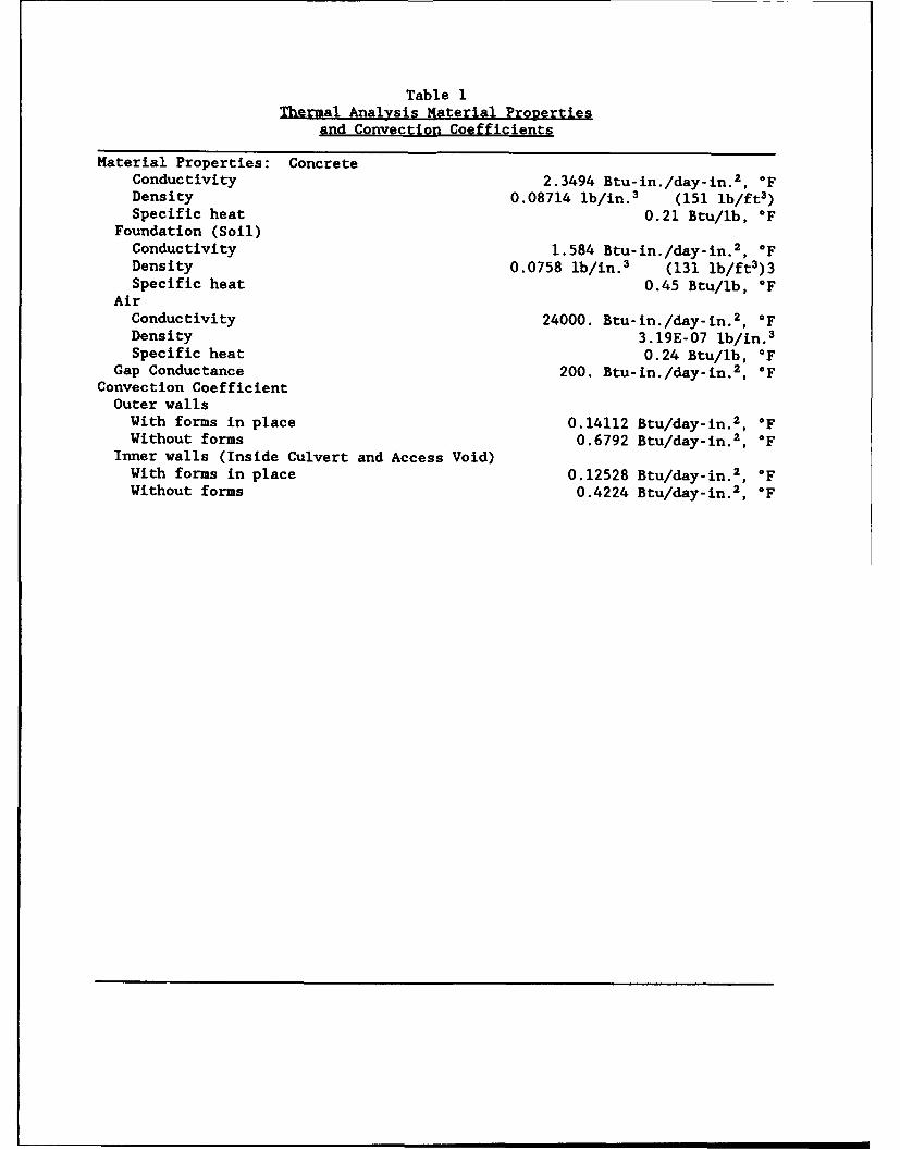
Table 1Thermal Analysis Material Properties
and Convection Coefficients
Material Properties: ConcreteConductivity 2.3494 Btu-in./day-in. 2 , OFDensity 0.08714 lb/in. 3 (151 lb/ft 3)Specific heat 0.21 Btu/lb, OF
Foundation (Soil)Conductivity 1.584 Btu-in./day-in. 2 , OFDensity 0.0758 lb/in. 3 (131 lb/ft 3)3Specific heat 0.45 Btu/lb, OF
AirConductivity 24000. Btu-in./day-in. 2 , OFDensity 3.19E-07 lb/in. 3
Specific heat 0.24 Btu/lb, °FGap Conductance 200. Btu-in./day-in. 2 , OF
Convection CoefficientOuter walls
With forms in place 0.14112 Btu/day-in. 2 , OFWithout forms 0.6792 Btu/day-in. 2 , °F
Inner walls (Inside Culvert and Access Void)With forms in place 0.12528 Btu/day-in. 2 , OFWithout forms 0.4224 Btu/day-in. 2 , OF
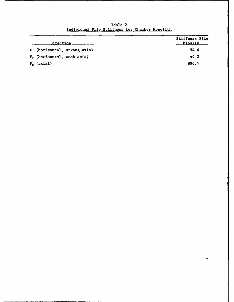
Table 2Individual Pile Stiffness for Chamber Monolith
Stiffness Pile
Direction kiDs/in.
F. (horizontal, strong axis) 54.6
F. (horizontal, weak axis) 44.2
F. (axial) 896.4
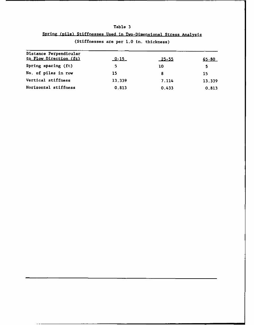
Table 3
Svrinz (Rile) Stiffnesses Used in Two-Dimensional Stress Analysis
(Stiffnesses are per 1.0 in. thickness)
Distance Perpendicular
to Flow Direction (ft) 0-15 25-55 65-80
Spring spacing (ft) 5 10 5
No. of piles in row 15 8 15
Vertical stiffness 13.339 7.114 13.339
Horizontal stiffness 0.813 0.433 0.813
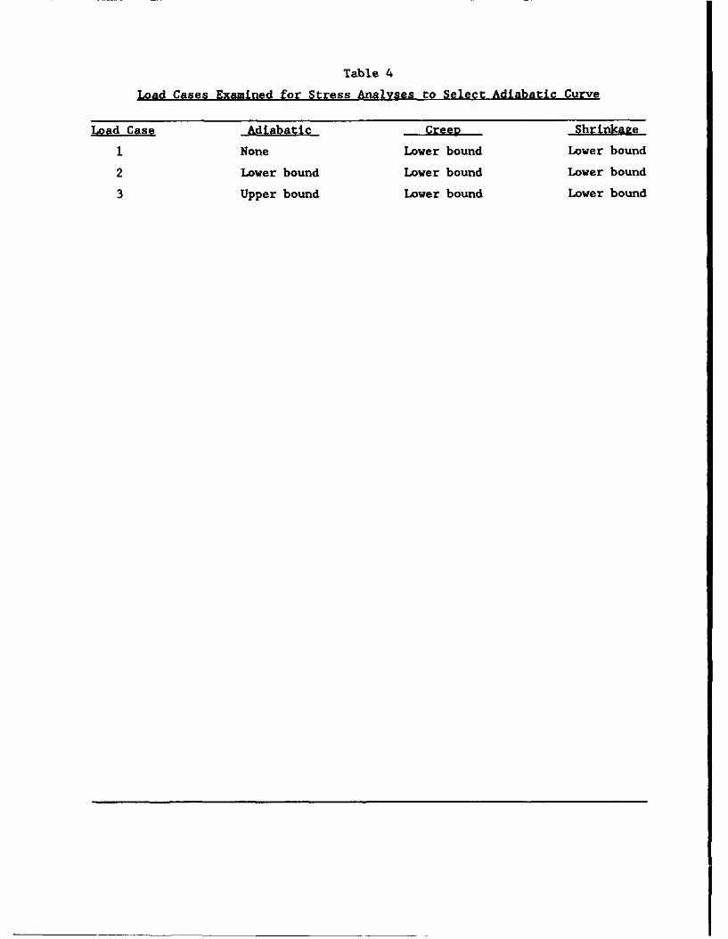
Table 4
Load Cases Examined for Stress Analyses to Select Adiabatic Curve
Load Case Adiabatic CreeR Shrinkage
1 None Lower bound Lower bound
2 Lower bound Lower bound Lower bound
3 Upper bound Lower bound Lower bound
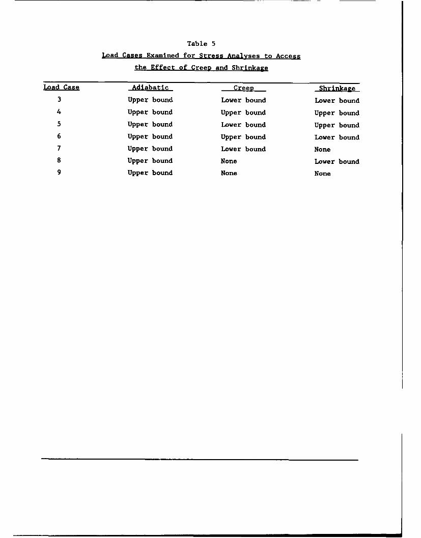
Table 5
Load Cases Examined for Stress Analyses to Access
the Effect of CreeR and Shrinkage
Load Case Adiabatic Creep Shrinkage
3 Upper bound Lower bound Lower bound
4 Upper bound Upper bound Upper bound5 Upper bound Lower bound Upper bound
6 Upper bound Upper bound Lower bound7 Upper bound Lower bound None
8 Upper bound None Lower bound9 Upper bound None None
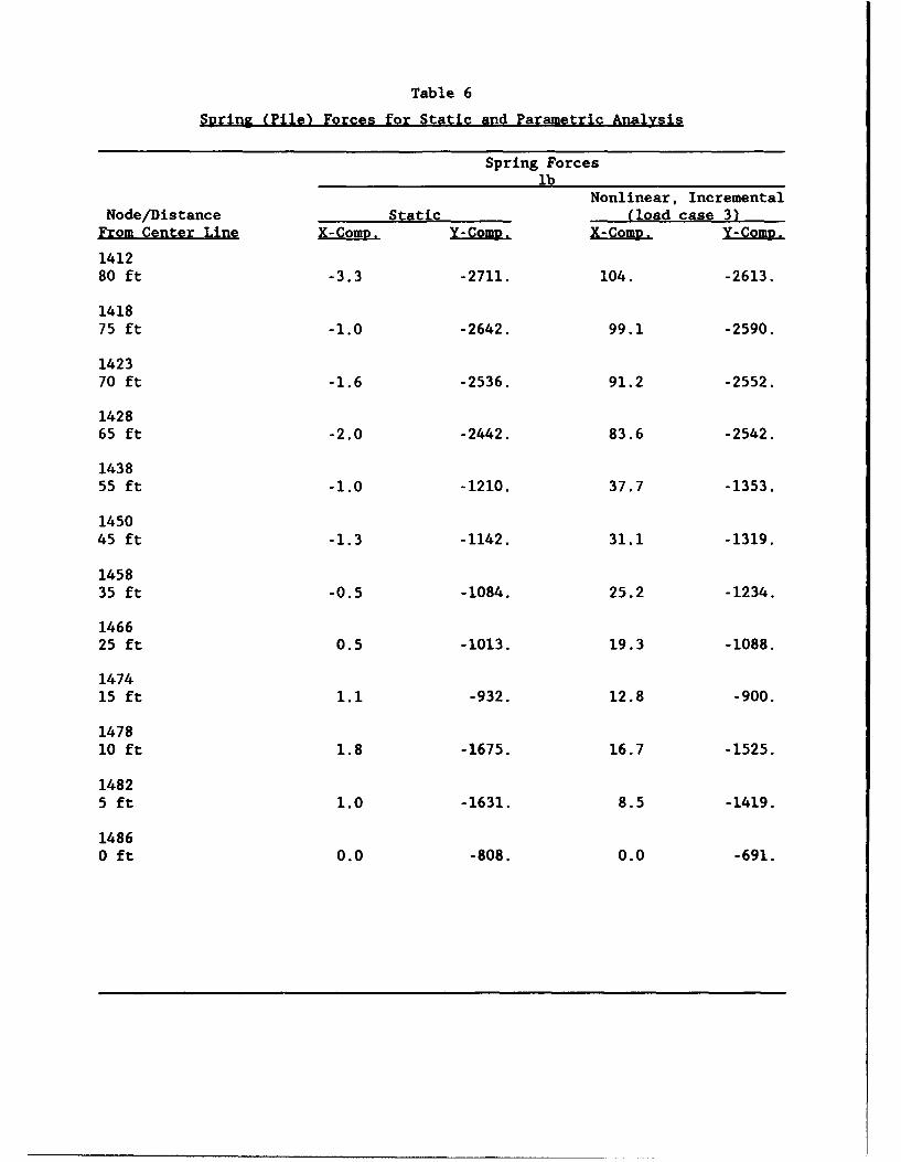
Table 6
Spring (Pile) Forces for Static and Parametric Analysis
Spring Forceslb
Nonlinear, IncrementalNode/Distance Static (load case 3)
From Center Line X-Comp. Y-ComR. X-ComR. X-ComR.
141280 ft -3.3 -2711. 104. -2613.
141875 ft -1.0 -2642. 99.1 -2590.
142370 ft -1.6 -2536. 91.2 -2552.
142865 ft -2.0 -2442. 83.6 -2542.
143855 ft -1.0 -1210. 37.7 -1353.
145045 ft -1.3 -1142. 31.1 -1319.
145835 ft -0.5 -1084. 25.2 -1234.
146625 ft 0.5 -1013. 19.3 -1088.
147415 ft 1.1 -932. 12.8 -900.
147810 ft 1.8 -1675. 16.7 -1525.
14825 ft 1.0 -1631. 8.5 -1419.
14860 ft 0.0 -808. 0.0 -691.
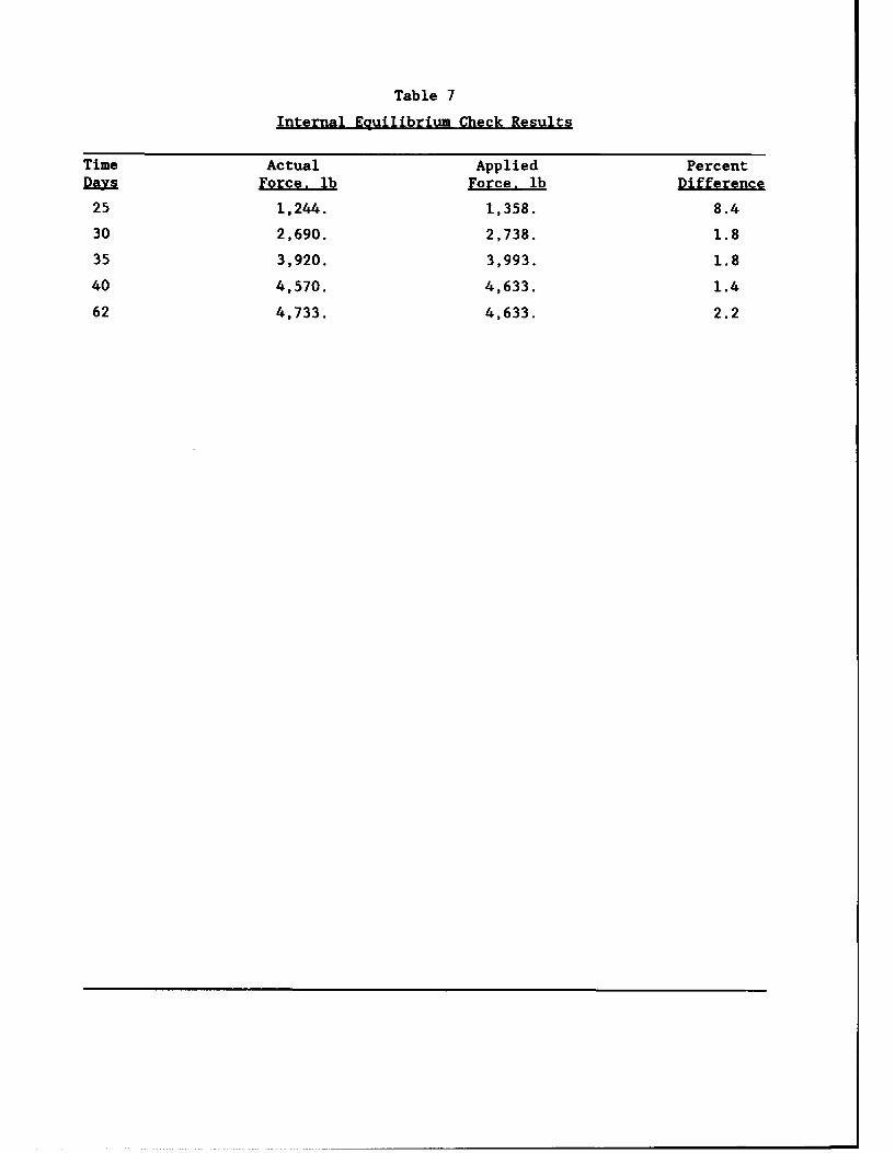
Table 7
Internal Equilibrium Check Results
Time Actual Applied PercentSForce. lb Force. lb Difference
25 1,244. 1,358. 8.4
30 2,690. 2,738. 1.8
35 3,920. 3,993. 1.8
40 4,570. 4,633. 1.4
62 4,733. 4,633. 2.2
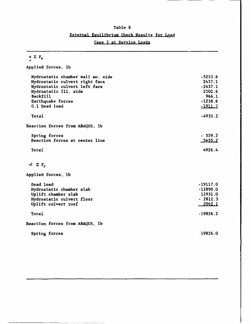
Table 8
External Eauilibrium Check Results for Load
Case 3 at Service Loads
Applied forces, lb
Hydrostatic chamber wall mo. side -5253.6Hydrostatic culvert right face 2437.1Hydrostatic culvert left face -2437.1Hydrostatic Ill. side 2502.6Backfill 966.1Earthquake forces -1238.60.1 Dead load -1911.7
Total -4935.2
Reaction forces from ABAQUS, lb
Spring forces - 529.2Reaction forces at center line 5455.2
Total 4926.4
+1 Z Fy
Applied forces, lb
Dead load -19117.0Hydrostatic chamber slab -12890.0Uplift chamber slab 12931.0Hydrostatic culvert floor - 2812.3Uplift culvert roof 2062.1
Total -19826.2
Reaction forces from ABAQUS, lb
Spring forces 19826.0
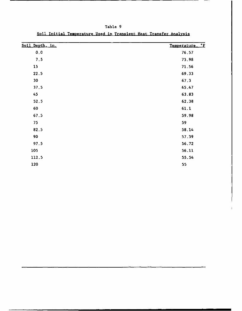
Table 9
Soil Initial Temperature Used in Transient Heat Transfer Analysis
Soil Depth, in, Temverature. *F
0.0 76.57
7.5 73.98
15 71.56
22.5 69.33
30 67.3
37.5 65.47
45 63.83
52.5 62.38
60 61.1
67.5 59.98
75 59
82.5 58.14
90 57.39
97.5 56.72
105 56.11
112.5 55.54
120 55
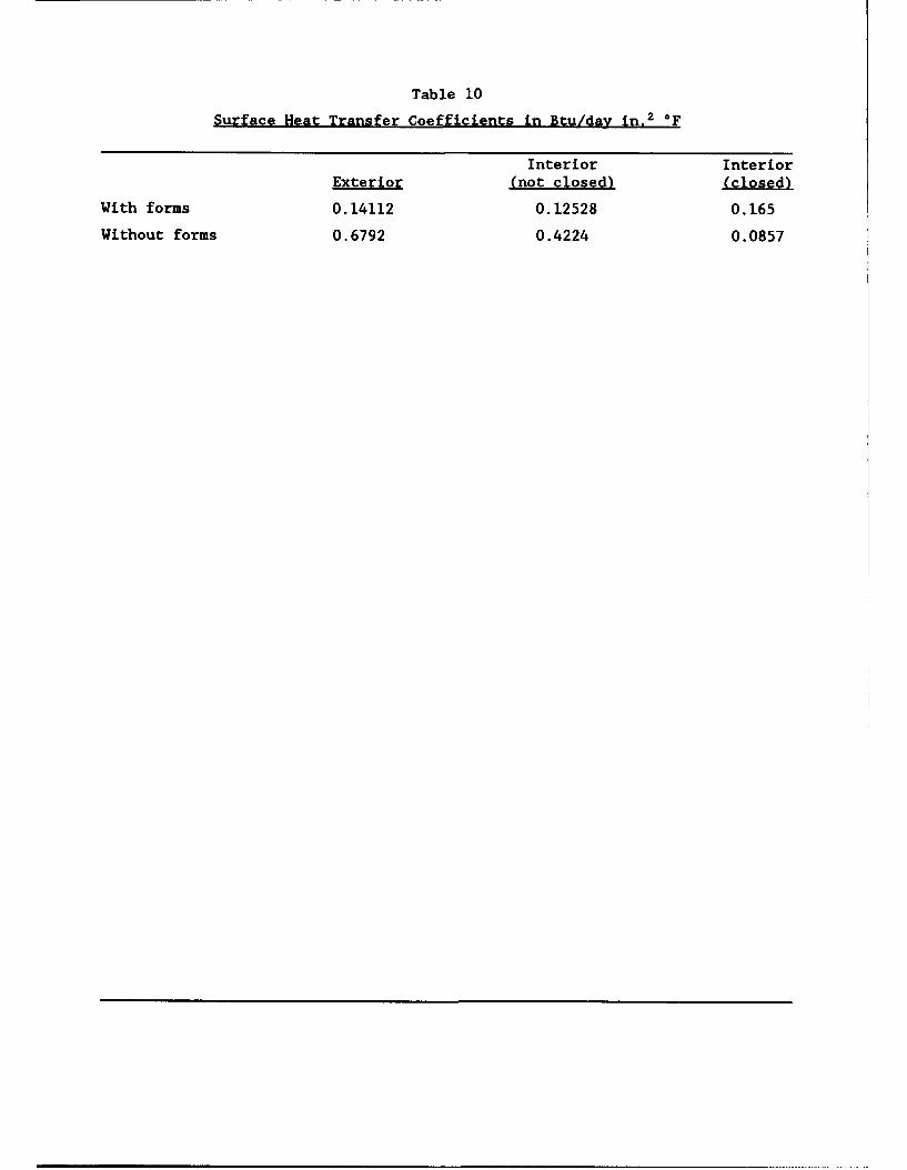
Table 10
Surface Heat Transfer Coefficients in Btu/day in. 2 oF
Interior Interior
Exterior (not closed) (closed)
With forms 0.14112 0.12528 0.165
Without forms 0.6792 0.4224 0.0857
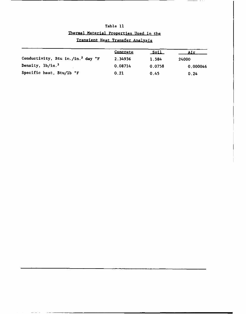
Table 11
Thermal Material Properties Used in the
Transient Heat Transfer Analysis
Concrete Soil Air
Conductivity, Btu in./in.2 day °F 2.34936 1.584 24000
Density, lb/in. 3 0.08714 0.0758 0.000046
Specific heat, Btu/lb °F 0.21 0.45 0.24
APPENDIX A: DEVELOPMENT OF TWO- AND THREE-DIMENSIONAL AGING
AND CREEP MODEL FOR CONCRETE (ANATECH, INC. 1987)
Purpose
1. The purpose of this work is to develop a computationally robust
constitutive model for aging concrete, considering creep, shrinkage, and
cracking for use in the ABAQUS code. The model parameters are quantified from
laboratory data for the elastic modulus as function of age, creep strain ver-
sus time, and shrinkage strain versus time. Two versions of this model are
considered: a two-dimensional version which can be applied to problems
involving plane stress, plane strain, and axisymmetric stress states; and an
unrestricted version for general three-dimensional stress states. The model-
ling of the cracking in both of these versions differ significantly from one
another--the three-dimensional case being far more complex in the computa-
tional details than its two-dimensional counterpart. This brief report
describes the main features of the constitutive model with respect to aging,
creep, and cracking.
Aging Effects in Concrete Creep
2. Figure Al shows a typical compliance curve (specific strain) for a
concrete cylinder loaded at age rO with stress ao . The vertical segment
of this curve represents the elastic strain per unit stress which is the
inverse of the elastic modulus. The curve represents the time-dependent
response of the cylinder which consists of a purely creep component (visco-
elastic) and a much smaller elastic component which is due to the aging elas-
tic recovery. It is impossible to separate these two components in the same
experiment; however, separate experiments for E(r) can be conducted and then
used to identify the purely creep part from the creep experiments. This,
however, is not usually done in practice, which becomes a source of error in
the predicted versus measured data. The measured curve J(t-r0 ) is usually
use directly in analysis for the creep component ec in the strain decomposi-
tion formula, which can be written as follows for the creep test:
Al
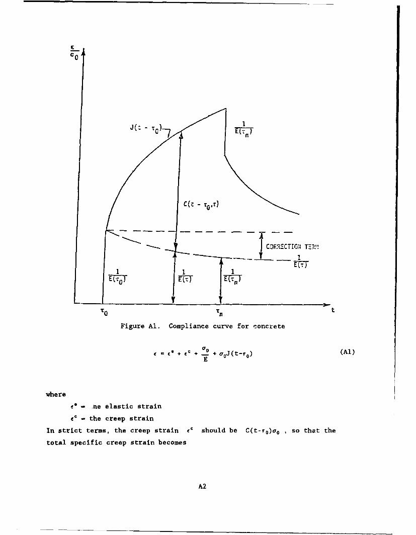
ECO
1
EJ( "
,TT)
""RRCTC TER t
E (
Figure Al. Compliance curve for concrete
= + e. + _ + o0J(t-.r) (Al)E
where
n ne elastic strain
e' the creep strain
In strict terms, the creep strain Ec should be C(t-r 0 )ao , so that the
total specific creep strain becomes
A2
1 1 + J(t-o) I + C(t-rO,) (A2)
As can be easily determined, J and C are the same for non-aging materials
and are nearly equal (within data scatter) for mature concrete. However, they
may differ significantly for very young concrete and, hence should be treated
separately.
3. If one plots in the same figure several creep curves for different
ages of loading, one obtains Figures A2 and A3. These curves differ from one
another in the elastic portion as well as the slope, as is illustrated in
Figure A3. Both of these differences are strictly due to aging, i.e., the
four curves shown in Figure A3 become one for nonaging materials and would
approach each other as the concrete's age increases.
Temperature Effects in Concrete Creep
4. Temperature affects concrete in a manner that is characteristic of
the so-called thermo-rheologically-simple material, but with the added effects
of aging. Thermo-rheologically-simple material is assumed to be nonaging.
For such material a creep curve at any temperature T , when plotted as func-
tion of log t, can be obtained from the creep curve at a base temperature To
by a simple shift along the log t axis as shown in Figure A4. The shift 0(t)
is usually referred to as the shift factor, and the log of 0(t) is called
the shift function.
5. The concept of thermo-rheologically-simple behavior is useful in
two respects: first, as a means to linearize the highly nonlinear strain-
stress hereditary integral; and second, as an extrapolation scheme to cover a
wide range of temperatures using only a few tests. It should be noted that,
in age of computer-based numerical analysis, numerical integration of nonlin-
ear integral equations can be c.complished just as easily in any form. How-
ever, the time-temperature equivalence principle can help explain the physical
behavior by illustrating the well-practiced concept of accelerated creep tests
in which long range creep data can be obtained by conducting creep tests at
higher temperature, but for a much shorter time.
A3
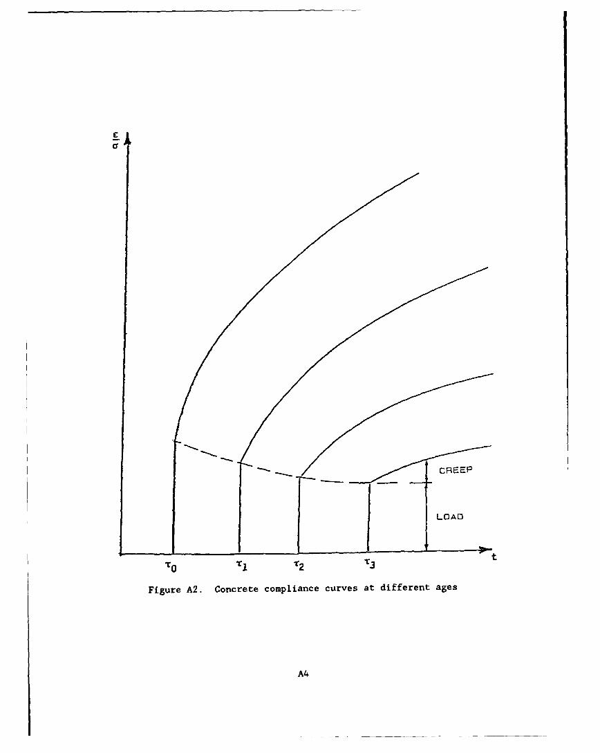
ýC R EEE-P
LOAD
T 0 Ti 2T
Figure A2. Concrete compliance curves at different ages
A4
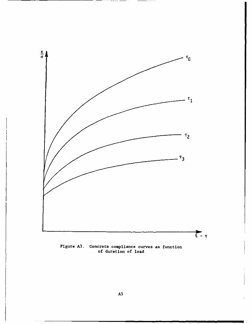
""I
Figure A3. Concrete compliance curves as functionof duration of load
A5
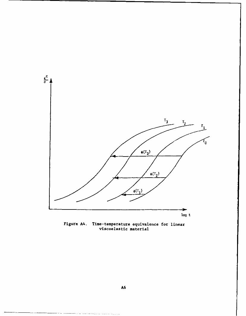
C
lo
TT
To
log t
Figure A4. Time-temperature equivalence for linearviscoelastic material
A6
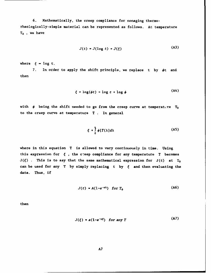
6. Mathematically, the creep compliance for nonaging thermo-
rheologically-simple material can be represented as follows. At temperature
To , we have
J(t) = J(log t) = J(Q) (A3)
where • - log t.
7. In order to apply the shift principle, we replace t by Ot and
then
= log(ot) = log t + log (A4)
with 4 being the shift needed to go from the creep curve at temperatcre To
to the creep curve at temperature T . In general
+ 4[T(X]dX (A5)0
where in this equation T is allowed to vary continuously in time. Using
this expression for ý , the creep compliance for any temperature T becomes
J(ý) . This is to say that the same mathematical expression for J(t) at To
can be used for any T by simply replacing t by ý and then evaluating the
data. Thus, if
J(t) - A(l-e-rt) for To (A6)
then
j(f) - a(l-e-r) for any T (A7)
A7
where
= [(A8)0
and 0 is obtained graphically from plots such as shown in Figure A4. This
process is not so straightforward for aging materials because the creep strain
depends not only on the duration of loading but also on the time at which the
load is applied. This implies that the shift factor becomes a function of
temperature and age.
8. Recalling the fact that temperature has a softening effect on
creep, which is akin to the rejuvenation of concrete, the time-temperature
equivalence principle can be extended to include the age of the material.
Assuming that aging of concrete is a logarithmically decreasing effect, we
introduce the concept of double shift: first shifting the base curve for
aging, and then shifting it again for temperatures. This is done as follows.
Let the base curve be J(t,r 0 ) for temperature To . If we plot this curve
on the log t axis, we have
J(t, To) = J1109 17] (A9)
where q - V(t-0).
9. We have now introduced the time shift factor q . Now introducing
the temperature shift factor, we have
J(t, ro, T) -f J [log 97(t-ro) + log 0(T)] J J[(t, ro)] (AIO)
where
ý(t,,r) - i7(t--ro)O(T) (All)
In general, for time varying temperature,
A8
t•(t, ) M O[T(A)] I8n(A-7) dA (A12)
and the creep compliance becomes
J(t,r,T) =J[et,t)] (A13)
The way to determine the time and temperature shift factor is: first place
the base curve obtained at age r0 on the log t-r axis: the curves for r,
r2 ,T3 ... plot below the base curve, as shown in Figure A5. The time
shift factor q(t-r) can then be determined by simply plotting the values of
q(t-r) , obtained graphically, versus r then fitting a formula to the curve.
Consider for example the formula:
J(t, r) - A(r)(1 - ert) (A14)
Then the curve for age r, becomes
J(t,Tl) - A(r 0 )(1 - e-rf(t•T)) (A15)
where e(t,r 1 ) - q(t - rj)
10. The next step is to determine the temperature shift factor O(T)
in the manner described previously. However, the assumption has to be made
that the temperature shift is independent of age, i.e., O(T) is the same for
all ages.
WES CreeR Relation
11. The creep relation for WES concrete is given below.
A9
mm mmm mm • amu u•mmI ~m In •ME • ON
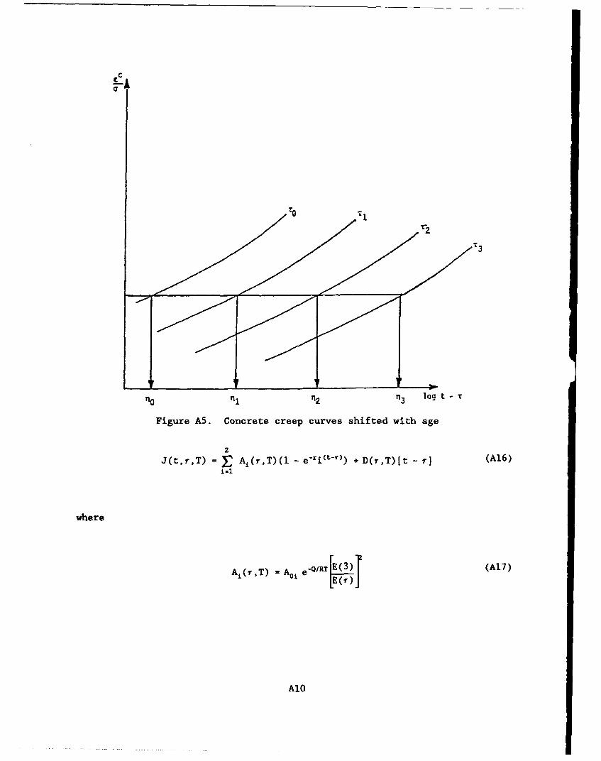
cc
no n n2 in3 log t -T
Figure A5. Concrete creep curves shifted with age
2
J(t,r,T) = • Ai(r,T)(I - e-ri(t-r)) + D(T,T)ft - r) (A16)I-1
where
Ai(r,T) - A0 1 e"Q/RT E (A17)
E()lJ
A10
E(r) - Eo + El(l - e-o1(r-1) + E2(1 - e-02(T-1) (A19)
Shrinkage is expressed as follows:
C= = C(1 - e Slt) + C2(1 - e-S2t) (A20)
The uniaxial strain-stress relation becomes
E(t) = d + J(t, r T dt + aT + (A21)Ir(W) JI a t)
The main features of the above relations are discussed below.
j. The creep formula is not the traditional logarithmic function,but it matches the available data. The linear term in Equa-tion A16 implies the presence of a viscous element which char-acterizes long term creep for metals. Its inclusion here ismotivated by accurate data fitting, not by physical consider-ations. Furthermore, the objection to this term is that it isnonaging. This is true only if the coefficient D is a con-stant, which is not the case here. The logarithmic formulafound its way in concrete creep because the term log(t - r+ 1) has a continuously deceasing slope; thus, it exhibits anaging phenomenon. The slope of the logarithmic formula isproportional to 1/(t -T + 1) , which is a decreasing functionof time. In our case, the slope of the linear term is propor-tional to l/E 2 (see Equation 19), which is an exponentiallydecreasing function of time. However, Equation 21 gives along-term strain that exhibits aging. It might be interestingin this regard to discuss Bazant's point and other workers inthe field who are similarly attached to the logarithmic for-mula. If we go back to Figure Al, we see that the measuredcreep compliance is J(t -to) , which is not the true creepcurve, although it is the curve that is usually plotted onsemi-log scale. However, as we discussed earlier, the truecreep compliance C(t - to) , which is usually ignored byexperimentalists, has an aging correction term as shown in thefigure. Notice that C(L - T0 ,r) is larger than J(t - o0)and the difference between the two curves become wider andwider with time. Therefore, if J(t - to) is a log function,then C(t-r 0 ,r) cannot be a log function any may in fact becloser to a linear function at long time. Also, there is evi-
All
dence that temperature eliminates the effect of aging, and atcertain temperatures concrete behaves like polymers. There-fore, it boils down to how one looks at the data. It shouldbe noted further that the present analysis is not limited bythe linear term in the creep formula and a third exponentialterm can be used instead. For example, the term (1 - e-
0.0 00 38
t)
can replace the linear term 3.8 x 10-It with little loss inaccuracy in the range of the data.
b. The first term in the series in Equation 16 governs the short-term creep for the first day; the second governs theintermediate-term creep, up to 30 days; and the last governsthe creep behavior beyond 30 days.
c. Aging is determined from the elastic modulus data and is rep-resented as an inverse square function, i.e., the creep strainis proportional to the square of the inverse of the elasticmodulus. This was determined by trial and error because oflack of data.
Crackinj
12. Cracking is assumed to occur when a cracking criterion is satis-
fied. This criterion consists of the following elements: (a) it is strain
driven but is modified by the stress, as will be shown later; (b) the crack
surface normal is in the direction of the principal strain; and (c) the crack-
ing criterion is interactive.
13. This criterion is implemented as follows. Consider a trace of the
two-dimensional failure surface shown in Figure A6 in principal stress space.
The ft and f. have the usual meaning, namely tensile and compressive
strength, respectively. For isotropic material, which describes concrete
prior to cracking, the principal strain and principal stress direction coin-
cide. Therefore, one could also express the cracking criterion in terms of
the principal strains. It is important to do so for concrete if we were to
predict cracking correctly. Consider, for example, a cube of material pres-
sure loaded with a2 . The cube will split, in the direction of the load,
under the effect of the el strain. The ai stress will be a small
A12
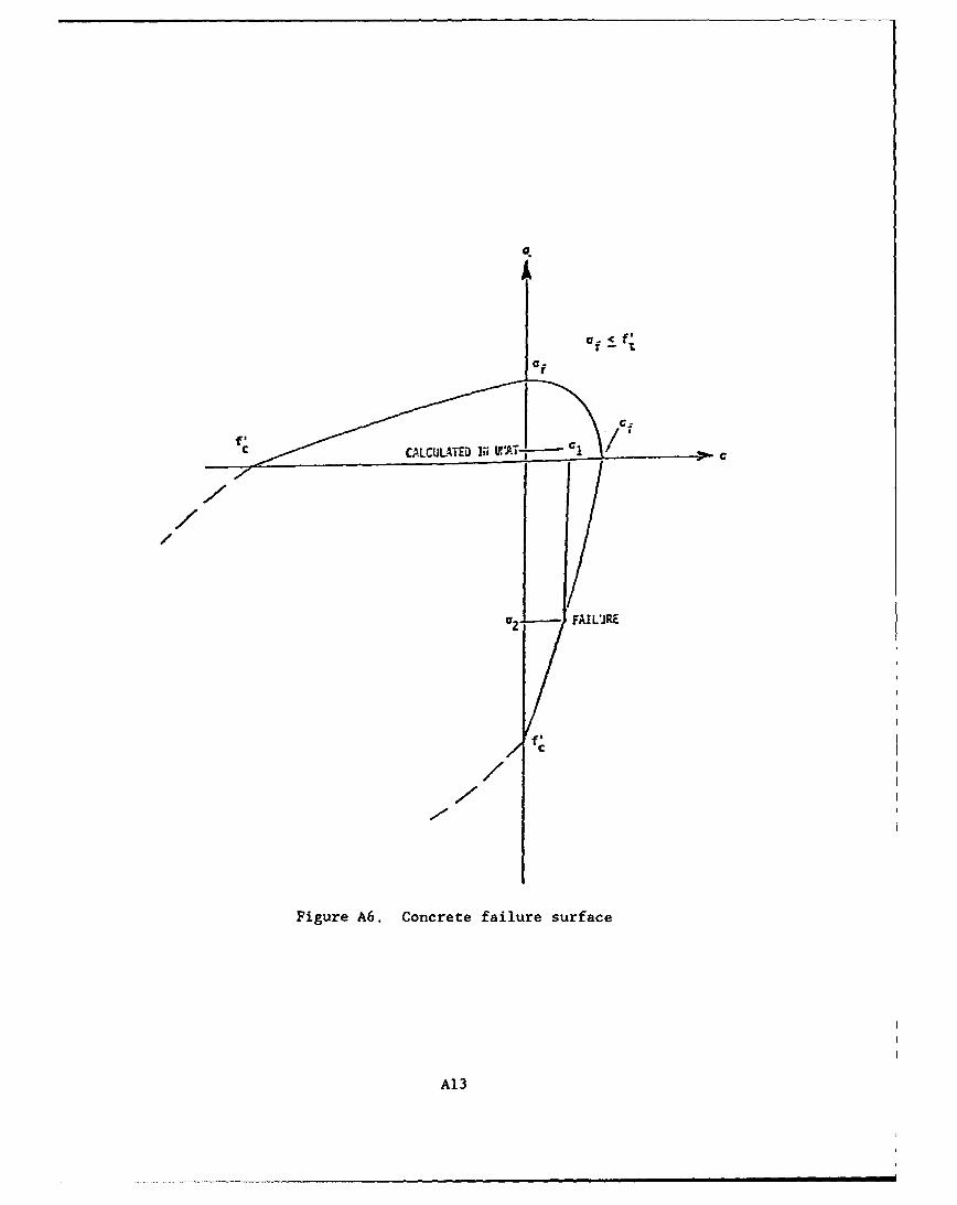
Of <fi
If
02 ' FAILIJPE
/ f •
//
Figure A6. Concrete failure surface
A13
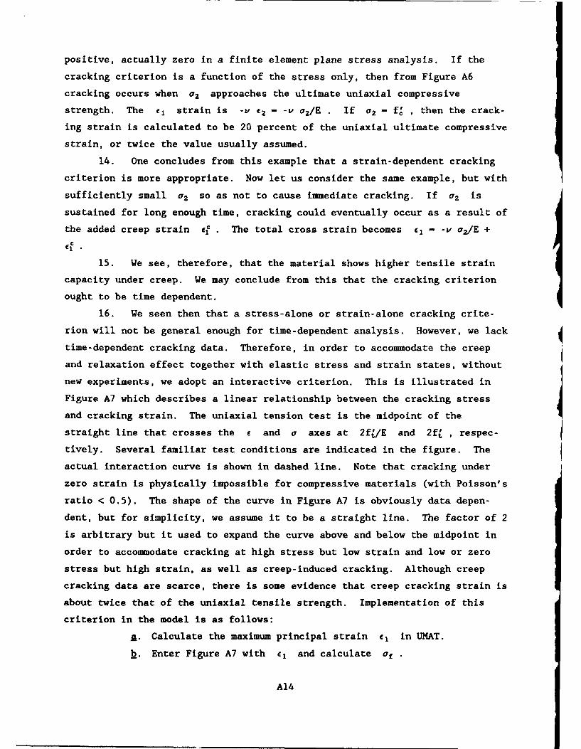
positive, actually zero in a finite element plane stress analysis. If the
cracking criterion is a function of the stress only, then from Figure A6
cracking occurs when 02 approaches the ultimate uniaxial compressive
strength. The el strain is -v C2 - -P o2/E . If a2 - f• , then the crack-
ing strain is calculated to be 20 percent of the uniaxial ultimate compressive
strain, or twice the value usually assumed.
14. One concludes from this example that a strain-dependent cracking
criterion is more appropriate. Now let us consider the same example, but with
sufficiently small a2 so as not to cause immediate cracking. If a2 is
sustained for long enough time, cracking could eventually occur as a result of
the added creep strain Ef . The total cross strain becomes el -v a2/E +
15. We see, therefore, that the material shows higher tensile strain
capacity under creep. We may conclude from this that the cracking criterion
ought to be time dependent.
16. We seen then that a stress-alone or strain-alone cracking crite-
rion will not be general enough for time-dependent analysis. However, we lack
time-dependent cracking data. Therefore, in order to accommodate the creep
and relaxation effect together with elastic stress and strain states, without
new experiments, we adopt an interactive criterion. This is illustrated in
Figure A7 which describes a linear relationship between the cracking stress
and cracking strain. The uniaxial tension test is the midpoint of the
straight line that crosses the c and a axes at 2ft/E and 2ft , respec-
tively. Several familiar test conditions are indicated in the figure. The
actual interaction curve is shown in dashed line. Note that cracking under
zero strain is physically impossible for compressive materials (with Poisson's
ratio < 0.5). The shape of the curve in Figure A7 is obviously data depen-
dent, but for simplicity, we assume it to be a straight line. The factor of 2
is arbitrary but it used to expand the curve above and below the midpoint in
order to accommodate cracking at high stress but low strain and low or zero
stress but high strain, as well as creep-induced cracking. Although creep
cracking data are scarce, there is some evidence that creep cracking strain is
about twice that of the uniaxial tensile strength. Implementation of this
criterion in the model is as follows:
A. Calculate the maximum principal strain el in UMAT.
k. Enter Figure A7 with el and calculate oa
A14
a
S 1 - ACTUAL
of = 2fI
(Assumed)
FCYLINDER SPLIT TEST
TRIAXIAL TENSION TEST
- BIAxIAL TENSiON TEST
(Oata)V f UNIAXIAL TENSILE STATIC TEST
f
UNIAXIAL COMPRESSIONfSPLIT TEST
\.•i /.- UNIAXIAL COMPRESSION,
/ SPLIT cREEP TEST
fi/E £j I f - 2fVE(Cal culated) (Ass "md)
in UMAT
Figure A7. Interactive fracture criterion for concrete
. Adjust the failure surface (Figure A6 amplitude, using af asthe intercept, instead of f.
d. Enter Figure A6 using the principal stresses a, and a 2 cal-
culated in UMAT, and calculate whether the (a,, a 2 ) point pene-
trates the failure surface. If so, introduce a crack whose
normal is in the principal strain direction and formulate theconstitutive matrix in the principal coordinate system.
e. Rotate the precracking stresses to the same coordinate system
and adjust these stresses to reflect the new cracking state.
f. Rotate the constitutive matrix and the stresses back to the
coordinate system of the structure.
g. The new constitutive matrix and stresses are then used byABAQUS to calculate the nodal forces and the tangent stiffness
matrix in the next step.
A15
Waterways Experiment Station Cataloglng-In-Publlcatlon Data
Truman, Kevin Z.Evaluation of thermal and incremental construction effects for mono-
liths AL-3 and AL-5 of the Melvin Price Locks and Dam / by Kevin Z.Truman, David J. Petruska, Abdelkader Ferhi ; prepared for Departmentof the Army, US Army Corps of Engineers.
382 p : ill.; 28 cm. -- (Contract report ; ITL-92-3)Includes bibliographical references.1. Structural optimization - Data processing. 2. Melvin Price Locks
and Dam (111.) 3. Concrete - Expansion and contraction. 4. Concrete --Creep. I. Petruska, David J. II. Ferhi, Abdelkader. III. United States.Army. Corps of Engineers. IV. U.S. Army Engineer Waterways Experi-ment Station. V. Computer-aided Structural Engineering Project. VI.Title. VII. Series: Contract report (U.S. Army Engineer Waterways Ex-periment Station) ; ITL-92-3.TA7 W34c no.ITL-92-3
WATERWAYS EXPERIMENT STATION REPORTSPUBLISHED UNDER THE COMPUTER-AIDED
STRUCTURAL ENGINEERING (CASE) PROJECT
Title Date
Technical Report K-78-1 List of Computer Programs for Computer-Aided Structural Engineering Feb 1978
Instruction Report 0-79-2 User's Guide: Computer Program with Interactive Graphics for Mar 1979
Analysis of Plane Frame Structures (CFRAME)
Technical Report K-80-1 Survey of Bridge-Oriented Design Software Jan 1980
Technical Report K-80-2 Evaluation of Computer Programs for the Design/Analysis of Jan 1980
Highway and Railway Bridges
Instruction Report K-80-1 User's Guide: Computer Program for Design/Review of Curvi- Feb 1980
linear Conduits/Culverts (CURCON)
Instruction Report K-80-3 A Three-Dimensional Finite Element Data Edit Program Mar 1980
Instruction Report K-80-4 A Three-Dimensional Stability Analysis/Design Program (3DSAD)Report 1: General Geometry Module Jun 1980
Report 3: General Analysis Module (CGAM) Jun 1982
Report 4: Special-Purpose Modules for Dams (CDAMS) Aug 1983
Instruction Report K-80-6 Basic User's Guide: Computer Program for Design and Analysis Dec 1980
of Inverted-T Retaining Walls and Floodwalls (TWDA)
Instruction Report K-80-7 User's Reference Manual: Computer Program for Design and Dec 1980
Analysis of Inverted-T Retaining Walls and Floodwalls (TWDA)
Technical Report K-80-4 Documentation of Finite Element AnalysesReport 1: Longview Outlet Works Conduit Dec 1980
Report 2: Anchored Wall Monolith, Bay Springs Lock Dec 1980
Technical Report K-80-5 Basic Pile Group Behavior Dec 1980
Instruction Report K-81-2 User's Guide: Computer Program for Design and Analysis of SheetPile Walls by Classical Methods (CSHTWAL)
Report 1: Computational Processes Feb 1981
Report 2: Interactive Graphics Options Mar 1981
Instruction Report K-81-3 Validation Report: Computer Program for Design and Analysis of Feb 1981
Inverted-T Retaining Walls and Floodwalls (rWDA)
Instruction Report K-81-4 Users Guide: Computer Program for Design and Analysis of Mar 1981
Cast-in-Place Tunnel Linings (NEWTUN)
Instruction Report K-81-6 User's Guide: Computer Program for Optimum Nonlinear Dynamic Mar 1981
Design of Reinforced Concrete Slabs Under Blast Loading(CBARCS)
Instruction Report K-81-7 User's Guide: Computer Program for Design or Investigation of Mar 1981
Orthogonal Culverts (CORTCUL)
Instruction Report K-81 -9 User's Guide: Computer Program for Three-Dimensional Analysis Aug 1981
of Building Systems (CTABS80)
Technical Report K-81-2 Theoretical Basis for CTABS80: A Computer Program for Sep 1981
Three-Dimensional Analysis of Building Systems
Instruction Report K-82-6 Users Guide: Computer Program for Analysis of Beam-Column Jun 1982
Structures with Nonlinear Supports (CBEAMC)
(Continued)
WATERWAYS EXPERIMENT STATION REPORTSPUBLISHED UNDER THE COMPUTER-AIDED
STRUCTURAL ENGINEERING (CASE) PROJECT
(Continued)
Title Date
Instruction Report K-82-7 User's Guide: Computer Program for Bearing Capacity Analysis Jun 1982of Shallow Foundations (CBEAR)
Instruction Report K-83-1 User's Guide: Computer Program with Interactive Graphics for Jan 1983Analysis of Plane Frame Structures (CFRAME)
Instruction Report K-83-2 User's Guide: Computer Program for Generation of Engineering Jun 1983Geometry (SKETCH)
Instruction Report K-83-5 User's Guide: Computer Program to Calculate Shear, Moment, Jul 1983and Thrust (CSMT) from Stress Results of a Two-DimensionalFinite Element Analysis
Technical Report K-83-1 Basic Pile Group Behavior Sep 1983
Technical Report K-83-3 Reference Manual: Computer Graphics Program for Generation of Sep 1983Engineering Geometry (SKETCH)
Technical Report K-83-4 Case Study of S;,5 Major General-Purpose Finite Element Programs Oct 1983
Instruction Report K-84-2 User's Guide: Computer Program for Optimum Dynamic Design Jan 1984of Nonlinear Metal Plates Under Blast Loading (CSDOOR)
Instruction Report K-84-7 User's Guide: Computer Program for Determining Induced Aug 1984Stresses and Consolidation Settlements (CSETT)
Instruction Report K-84-8 Seepage Analysis of Confined Flow Problems by the Method of Sep 1984Fragments (CFRAG)
Instruction Report K-84-11 User's Guide for Computer Program CGFAG, Concrete General Sep 1984Flexure Analysis with Graphics
Technical Report K-84-3 Computer-Aided Drafting and Design for Corps Structural Oct 1984Engineers
Technical Report ATC-86-5 Decision Logic Table Formulation of ACI 318-77, Building Code Jun 1986Requirements for Reinforced Concrete for Automated Con-straint Processing, Volumes I and II
Technical Report ITL-87-2 A Case Committee Study of Finite Element Analysis of Concrete Jan 1987Flat Slabs
Instruction Report ITL-87-1 User's Guide: Computer Program for Two-Dimensional Analysis Apr 1987of U-Frame Structures (CUFRAM)
Instruction Report ITL-87-2 User's Guide: For Concrete Strength Investigation and Design May 1987(CASTR) in Accordance with ACI 318-83
Technical Report ITL-87-6 Finite-Element MWhod Package for Solving Steady-State Seepage May 1987Problems
Instruction Report ITL-87-3 User's Guide: A Three Dimensional Stability Analysis/Design Jun 1987Program (3DSAD) Module
Report 1: Revision 1: General Geometry Jun 1987Report 2: General Loads Module Sep 1989Report 6: Free-Body Module Sep 1989
(Continued)
WATERWAYS EXPERIMENT STATION REPORTSPUBLISHED UNDER THE COMPUTER-AIDED
STRUCTURAL ENGINEERING (CASE) PROJECT
(Continued)Title Date
Instruction Report ITL-87-4 User's Guide: 2-D Frame Analysis Link Program (LINK2D) Jun 1987
Technical Report ITL-87-4 Finite Element Studies of a Horizontally Framed Miter Gate Aug 1987Report 1: Initial and Refined Finite Element Models (Phases
A, B, and C), Volumes I and IIReport 2: Simplified Frame Model (Phase D)Report 3: Alternate Configuration Miter Gate Finite Element
Studies-Open SectionReport 4: Alternate Configuration Miter Gate Finite Element
Studies-Closed SectionsReport 5: Alternate Configuration Miter Gate Finite Element
Studies-Additional Closed SectionsReport 6: Elastic Bucklinn of Girders in Horizontally Framed
Miter Gate,Report 7: Application and Summary
Instruction Report GL-87-1 User's Guide: UTEXAS2 Slope-Stability Package; Volume I, Aug 1987User's Manual
Instruction Report ITL-87-5 Sliding Stability of Concrete Structures (CSLIDE) Oct 1987
Instruction Report ITL-87-6 Cr; dfia Specifications for and Validation of a Computer Program Dec 1987for the Design or Investigation of Horizontally Framed MiterGates (CMITER)
Technical Report ITL-87-8 Procedure for Static Analysis of Gravity Dams Using the Finite Jan 1988Element Method - Phase 1 a
Instruction Report ITL-88-1 User's Guide: Computer Program for Analysis of Planar Grid Feb 1988Structures (CGRID)
Technical Report ITL-88-1 Development of Design Formulas for Ribbed Mat Foundations Apr 1988on Expansive Soils
Technical Report ITL-88-2 User's Guide: Pile Group Graphics Display (CPGG) Post- Apr 1988.processor to CPGA Program
Instruction Report ITL-88-2 User's Guide for Design and Investigation of Horizontally Framed Jun 1988Miter Gates (CMITER)
Instruction Report ITL-88-4 User's Guide for Revised Computer Program to Calculate Shear, Sep 1988Moment, and Thrust (CSMT)
Instruction Report GL-87-1 User's Guide: UTEXAS2 Slope-Stability Package; Volume II, Feb 1989Theory
Technical Report ITL-89-3 User's Guide: Pile Group Analysis (CPGA) Computer Group Jul 1989
Technical Report ITL-89-4 CBASIN-Structural Design of Saint Anthony Falls Stilling Basins Aug 1989According to Corps of Engineers Criteria for HydraulicStructures; Computer Program X0098
(Continued)
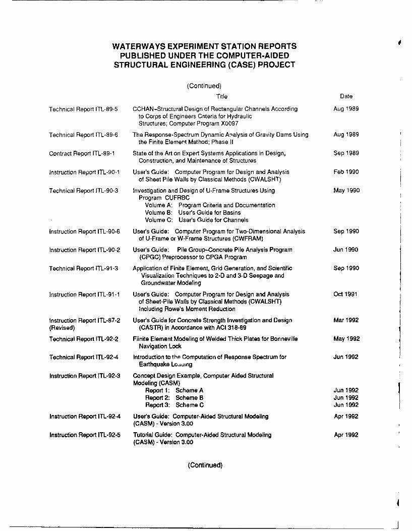
WATERWAYS EXPERIMENT STATION REPORTSPUBLISHED UNDER THE COMPUTER-AIDED
STRUCTURAL ENGINEERING (CASE) PROJECT
(Continued)
Title Date
Technical Report ITL-89-5 CCHAN-Structural Design of Rectangular Channels According Aug 1989to Corps of Engineers Criteria for HydraulicStructures; Computer Program X0097
Technical Report ITL-89-6 The Response-Spectrum Dynamic Analysis of Gravity Dams Using Aug 1989the Finite Element Method; Phase II
Contract Report ITL-89-1 State of the Art on Expert Systems Applications in Design, Sep 1989Construction, and Maintenance of Structures
Instruction Report ITL-90-1 User's Guide: Computer Program for Design and Analysis Feb 1990of Sheet Pile Walls by Classical Methods (CWALSHT)
Technical Report ITL-90-3 Investigation and Design of U-Frame Structures Using May 1990Program CUFRBC
Volume A: Program Criteria and DocumentationVolume B: User's Guide for BasinsVolume C: User's Guide for Channels
Instruction Report ITL-90-6 Users Guide: Computer Program for Two-Dimensional Analysis Sep 1990of U-Frame or W-Frame Structures (CWFRAM)
Instruction Report ITL-90-2 User's Guide: Pile Group-Concrete Pile Analysis Program Jun 1990(CPGC) Preprocessor to CPGA Program
Technical Report ITL-91-3 Application of Finite Element, Grid Generation, and Scientific Sep 1990Visualization Techniques to 2-D and 3-D Seepage andGroundwater Modeling
Instruction Report ITL-91-1 Users Guide: Computer Program for Design and Analysis Oct 1991of Sheet-Pile Walls by Classical Methods (CWALSHT)Including Rowe's Moment Reduction
Instruction Report ITL-87-2 Users Guide for Concrete Strength Investigation and Design Mar 1992(Revised) (CASTR) in Accordance with ACI 318-89
Technical Report ITL-92-2 Fiinite Element Modeling of Welded Thick Plates for Bonneville May 1992Navigation Lock
Technical Report ITL-92-4 Introduction to thp Computation of Response Spectrum for Jun 1992Earthquake Louing
Instruction Report ITL-92-3 Concept Design Example, Computer Aided StructuralModeling (CASM)
Report 1: Scheme A Jun 1992Report 2: Scheme B Jun 1992Report 3: Scheme C Jun 1992
Instruction Report ITL-92-4 User's Guide: Computer-Aided Structural Modeling Apr 1992(CASM) - Version 3.00
Instruction Report ITL-92-5 Tutorial Guide: Computer-Aided Structural Modeling Apr 1992(CASM) - Version 3.00
(Continued)
j
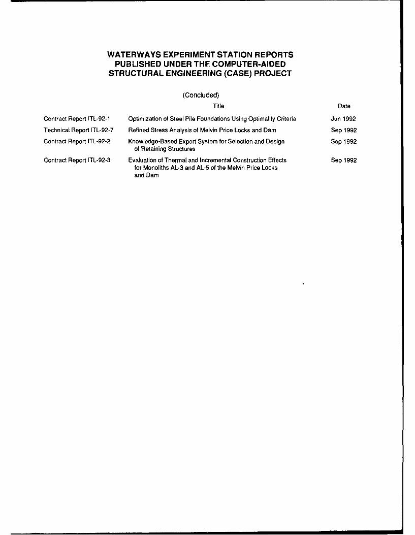
WATERWAYS EXPERIMENT STATION REPORTSPUBLISHED UNDER THE COMPUTER-AIDED
STRUCTURAL ENGINEERING (CASE) PROJECT
(Concluded)
Title Date
Contract Report ITL-92-1 Optimization of Steel Pile Foundations Using Optimality Criteria Jun 1992
Technical Report ITL-92-7 Refined Stress Analysis of Melvin Price Locks and Dam Sep 1992
Contract Report ITL-92-2 Knowledge-Based Expert System for Selection and Design Sep 1992of Retaining Structures
Contract Report ITL-92-3 Evaluation of Thermal and Incremental Construction Effects Sep 1992for Monoliths AL-3 and AL-5 of the Melvin Price Locksand Dam
Top Related