


Languages
Pages
Legal


1
Address Correspondence to:
Lowell L. Getz2113 Lynwood Dr.Champaign, IL 61821-6606Phone: (217) 356-5767
RH: Getz et al. – Home ranges of voles
Home range dynamics of sympatric vole populations: influence of food
resources, population density, interspecific
competition, and mating system
Lowell L. Getz*, Joyce E. Hofmann, Betty McGuire
and Madan K. Oli
Department of Animal Biology, University of Illinois, 505 S. Goodwin
Ave., Urbana, IL 61801, USA (LLG)
Illinois Natural History Survey, 607 E. Peabody Dr.,
Champaign, IL 81820, USA (JEH)
Department of Biological Sciences, Smith College,
Northampton, MA 01063, USA (BM)
Department of Wildlife Ecology and Conservation, 110 Newins-Ziegler
Hall, University of Florida, Gainesville, FL 32611, USA (MKO)
* Coresspondent: [email protected]
2
We studied variation in home range size in fluctuating populations of
Microtus ochrogaster and M. pennsylvanicus in alfalfa, bluegrass and
tallgrass habitats over a 25-year period in east-central Illinois. The
three habitats differed in food availability and vegetative cover.
Home range indices of both species were complexly related to abundance
of food resources. Home ranges of M. ochrogaster were smallest in the
high food habitat (alfalfa), largest in the low food habitat
(tallgrass) and intermediate in medium food habitat (bluegrass). M.
pennsylvanicus home ranges were largest in the low food habitat, but
did not differ between the high and intermediate food habitats. M.
ochrogaster did not have smaller home ranges in supplementally fed
medium and low food habitats; those of M. pennsylvanicus were smaller
only in the low food habitat. Home ranges of M. ochrogaster were
compressed only at population densities above 100/ha, irrespective of
food levels; those of M. pennsylvanicus were smaller at high densities
only in medium and low food habitats. Presence of the other species
did not influence size of home ranges of either species. Within-
habitat seasonal variation in home range indices indicated a
confounding response to cover (prey risk) and food. Home ranges of all
age classes of M. pennsylvanicus were larger than those of M.
ochrogaster in all three habitats. There was no obvious relationship
between home range sizes of adult males and females in relation to the
mating system of each species. For both species in all three habitats,
home ranges of adult males were larger than those of adult females.
Key words: home range, Microtus ochrogaster, Microtus pennsylvanicus,
voles
3
An understanding of variation in home range size of small
mammals, and factors responsible for such variation, is important to
demographic studies within and among habitats. The manner in which
individuals respond to environmental influences by increasing or
decreasing their range of movements provides evidence for the role of
given variables in demography of species. A number of factors
potentially influence the area over which an individual moves in its
day-to-day activities, i.e., its home range. Variation in distribution
and abundance of food and other resources (e.g., cover, nest sites) may
influence habitat-specific and seasonal differences in size of home
ranges.
At higher population densities, competition for space and
resources may result in compression of home range size (Mares et al.
1982; Vincent et al. 1995; Oli et al. 2002). When two competing
species occupy a site, interspecific interactions may result in
contraction of home ranges of one or both species.
The amount of area over which an individual must range to obtain
sufficient food is an especially important determinant of home range
size for many species (Meserve 1971; Slade et al. 1997; Abramsky and
Tracy 1980; Taitt and Krebs 1981; Ims 1987; Mares and Lacher 1987;
Boutin 1990; Desy et al. 1990; Jones 1990; Akbar and Gorman 1993;
Fortier and Tamarin 1998; Fortier et al. 2001). Further, several
studies have shown that as population density changes, presumably
altering levels of competition for space and resources, so too may home
range size (Abramsky and Tracy 1980; Gaines and Johnson 1982; Rodd and
Boonstra 1984; Ostfeld and Canham 1995; Fortier and Tamarin 1998; Hubbs
and Boonstra 1998). However, other studies (Lacki et al. 1984; Wolff
1985; Mares and Lacher 1987) found no such relationship between food
availability and population density.
4
Anderson (1986) and Desy et al. (1990) found home ranges of some
species of arvicoline rodents to be smaller in sites where the risk of
predation is greater, i.e., habitats with sparse cover.
Schmidt et al. (2002) reported a positive relationship between
home range size male, but not female, body mass in Dicrostonyz
groenlandicus. However, food availability confounded the relationship
between body mass and home range size of females.
Home range size also may vary with reproductive tactics of the
sexes. Gaulin and Fitzgerald (1988) found that in species displaying
promiscuous/polygynous mating systems (e.g., Microtus pennsylvanicus),
males had larger home ranges than did females, owing to male-male
competition for mates. They further found that home range sizes did
not differ between the sexes in monogamous/communal nesting species
(e.g., M. ochrogaster). On the other hand, Meserve (1971) and Swihart
and Slade (1989) found home ranges of male M. ochrogaster to be larger
than those of females. Getz et al. (1993) reported that 45% of the
adult males in M. ochrogaster populations were not residents at nests
of male-female pairs or communal groups, and wandered within the study
site. Inclusion of these males in the analyses may result in biased
results regarding home range sizes of male M. ochrogaster.
Reliable estimates of small mammal home ranges are difficult to
achieve. Considerable effort is required to delimit precisely the
boundaries of the area an individual occupies, whether by indirect
measures such as radio telemetry or by direct observation (Jones and
Sherman 1983; Ribble et al. 2002). A commonly employed alternative
method of estimating home range size includes plotting capture
locations from grid live-trapping and estimating the area encompassed
by the study animals (Hayne 1949, 1950). Because grid stations do not
correspond to the boundaries of individual home ranges, considerable
5
variability is inherent in such measures. All too often, trapping
protocols result in only 3-5 captures of a given individual, rendering
such data more or less anecdotal (Krohne 1986). Less precise indirect
means of estimating home range size include measuring distances between
captures, either between the first two captures or the maximum distance
between all captures during a given trapping session (Gaines and
Johnson 1982 Slade and Swihart 1983; Slade and Russell 1998). Because
most field studies of arvicoline rodents are of limited duration (1-5
years; Taitt and Krebs 1985), the quantity of data available for
estimating home ranges is limited. Small sample sizes, combined with
the imprecision of estimates and variability in home range size, limit
analyses of home range data.
In this paper we present home range data obtained during the
course of a 25-year study of the prairie vole, Microtus ochrogaster,
and meadow vole, M. pennsylvanicus (Getz et al. 2001). Populations of
the two species in three different habitats were monitored monthly,
year-round. The habitats differed in food availability and seasonal
changes in cover. As a result of the scope and duration of the study,
we obtained sufficiently large sample sizes of home range indices (M.
ochrogaster, >12,000; M. pennsylvanicus, >5,000) to test hypotheses
regarding variation in home range size and demographic implications.
In addition, we analyzed home range data from two shorter term
manipulative studies involving supplemental feeding and interspecific
interactions.
We tested the following predictions: (1) home ranges are smaller
where (habitats) and when (seasons) food is more abundant, (2) there is
a negative relationship between home range size and population density,
(3) interspecific competition between two sympatric species will result
in smaller home ranges of one or both, (4) home range sizes will be

6
smaller when risk of predation is greatest, and (5) home ranges reflect
mating tactics of the species. We also evaluated the importance of
variation in home range size in understanding the demography of the two
species.
Methods
Study sites.--The study sites were located in the University of
Illinois Biological Research Area (“Phillips Tract”) and Trelease
Prairie, both 6 km NE of Urbana, Illinois (40º15’N, 88º28’W). For the
long term study, populations of M. ochrogaster and M. pennsylvanicus
were monitored monthly in 3 habitats: restored tallgrass prairie (March
1972--May 1997), bluegrass, Poa pratensis (January 1972--May 1997), and
alfalfa, Medicago sativa (May 1972--May 1997; Getz et al. 1987, 2001).
Tallgrass prairie was the original habitat of both species in Illinois,
and bluegrass, an introduced species, represents 1 of the more common
habitats in which the 2 species can be found today in Illinois.
Alfalfa is an atypical habitat that provides exceptionally high-quality
food for both species (Cole and Batzli 1979; Lindroth and Batzli 1984).
We trapped study sites in 2 restored tallgrass prairies, 1
located in Trelease Prairie, the other in Phillips Tract (Getz et al.
1987). Trelease Prairie, established in 1944, was bordered by a mowed
lawn, cultivated fields, a forest, and a macadam county road. Relative
abundances of plants in Trelease Prairie were as follows: big bluestem,
Andropogon gerardii (17%); bush clover, Lespedeza cuneata (16%);
ironweed, Vernonia (12%); Indian grass, Sorghastrum nutans (10%);
milkweed, Asclepias (9%); goldenrod, Solidago (9%); Poa pratensis (5%);
switch grass, Panicum (5%); blackberry, Rubus (2%); little bluestem, A.
scoparius (2%); about 10 other species with relative abundances of <1%
(Getz et al. 1979).

7
The tallgrass prairie in the Phillips Tract was established in
1968. The site was bordered on 1 side by an abandoned field that
underwent succession from forbs and grasses to shrubs and small trees
by the time the study ended. Cultivated fields bordered the other 3
sides. When the Phillips Tract site was first trapped in September
1977, prairie vegetation was well-developed. Lindroth and Batzli
(1984) recorded relative abundances of the most prominent plant species
in that site: A. gerardii, (38%); Lespedeza cuneata (25%); Beard tongue
foxglove, Penstemon digitalis (16%); and S. nutans (19%). All other
species represented <1% relative abundance. Both prairies were burned
during the spring at 3-4 year intervals to retard invading shrubs and
trees.
The bluegrass study sites were established within a former
bluegrass pasture located in Phillips Tract. The pasture was released
from grazing in June 1971; dense vegetative cover existed by autumn
1971. Relative abundances of plants during that period were: P.
pratensis (70%); dandelion, Taraxacum officinale (14%); wild parsnip,
Pastinaca sativa (4%); goatsbeard, Tragopogon (3%); about 20 other
species with relative abundances of <1% (Getz et al. 1979).
To reduce successional changes, especially invading forbs, shrubs
and trees, the bluegrass sites were mowed during late summer every 2-3
years. The entire area was mowed at the same time. A rotary mower was
set to cut the vegetation about 25 cm above the surface. That height
resulted in suppression of growth of the invading forbs and woody
vegetation, but left the bluegrass uncut.
Two adjacent sites with M. sativa were trapped during the study.
A site was trapped until the M. sativa began to be crowded out by
invading forbs and grasses. One year before trapping was terminated in
1 site, M. sativa was planted in the other site so that the plants
8
would be fully developed when trapping commenced in that site. Sites
were separated by a 10-m closely mown strip. The strip reduced the
incidence of animals having home ranges that included parts of the two
study ssites when M. sativa was present in both fields. Initially, M.
sativa comprised 75% of the vegetation in each site. During the last
year of usage, other common plants included P. pratensis, Solidago,
Phleum pratense, Bromus inermis, clover (Trifolium repens and T.
pratense), and plantain (Plantago). A series of 3-m wide strips were
mowed (every 3rd strip) 25 cm above the surface periodically each summer
to control invading weedy forbs and promote new growth of M. sativa.
The first strips usually were mowed in early June; mowing normally
stopped in mid September. The subsequent strips were not mowed until
vegetation in the previously mowed strips was nearly full-grown. Times
of mowing were spaced so that at least two-thirds of the field had
vegetative cover at all times.
Trapping procedures.--A grid system with 10-m intervals was
established in all study sites. One wooden multiple-capture live-trap
(Burt 1940) was placed at each station. Each month a 2-day prebaiting
period was followed by a 3-day trapping session. Cracked corn was used
for prebaiting and as bait in the traps. We used vegetation or
aluminum shields to protect the traps from the sun during the summer.
The wooden traps provided ample insulation in the winter making
provision of nesting material unnecessary. We estimated trap mortality
to be less than 0.5% during the study.
Traps were set in the afternoon and checked at approximately 0800
h and 1500 h the following 3 days. All animals were toe-clipped at
first capture for individual identification (maximum of 2 toes on each
foot). Although toe clipping no longer is a recommended method of
marking animals, during most of the time of the study, few alternative
9
methods were available. Ear tags were available, but owing to frequent
loss of tags, toe clipping was deemed a more effective means of marking
individuals. The field protocol, including use of toe clipping, was
reviewed periodically by the University of Illinois Laboratory Animal
Resource Committee throughout the study. The committee approved the
field protocol based on University and Federal guidelines, as well as
those recommended by the American Society of Mammalogists, in effect at
the time
Species, grid station, individual identification, sex, and body
mass to the nearest 1 g were recorded at each capture. For analysis,
animals were grouped by age based on body mass: > 30 g, adult;
subadult, 20-29 g; and juvenile, < 19 g.
Manipulative studies
We conducted two manipulative studies to examine the influences
of food availability and interspecific interactions on demography and
population fluctuations of the two species. Home range indices were
calculated for these data sets. Trapping procedures were as described
above.
Supplemental feeding.--A 0.5 ha bluegrass study site was
supplementally fed from June 1977 through December 1983 (Getz et al.
1987). A 0.5 ha tallgrass site was supplementally fed from September
1977 through May 1987. Feeding stations, consisting of 0.5 liter glass
bottles, were placed at each trapping station. Purina rabbit chow (No.
5321), a high quality diet for both M. ochrogaster and M.
pennsylvanicus (Cole and Batzli 1979), was used as supplemental food.
The bottles were checked twice weekly and refilled as necessary to
ensure food was present in them and in good condition at all times.

10
Interspecific interaction.--Effects of presence of one species on
the other were examined in both bluegrass and tallgrass. All M.
pennsylvanicus were removed from a 1.0 ha bluegrass site each trapping
session from May 1977 through May 1997. M. ochrogaster were removed
from another 1.0 ha bluegrass site from May 1977 through May 1987.
Because M. ochrogaster populations were very low and M. pennsylvanicus
very high most of the time in tallgrass (Getz et al. 2001), only
effects of the latter on M. ochrogaster were tested in tallgrass. M.
pennsylvanicus were removed from a 0.5 ha tallgrass site from September
1984 through May 1997. All animals removed from a site were released
on the opposite side of an Interstate highway, approximately 1 km from
the study sites.
Data analysis
We used the minimum number alive method to estimate population
density for each trapping session (Krebs 1966). Previously marked
individuals not captured in a given trapping session, but captured in a
subsequent session, were considered to have been present during the
sessions in which they were not captured. Although the Jolly-Seber
index is recommended for estimating population density (Efford 1992),
at least 10 individuals must be trapped each session in order to obtain
reasonable estimates (Pollock, et al. 1990). During months voles were
present in the study sites, 10 or fewer M. ochrogaster were trapped
26%, 52% and 62% percent of trapping sessions in alfalfa, bluegrass,
and tallgrass, respectively. Ten or fewer M. pennsylvanicus were
trapped 55% of the sessions in alfalfa, 46% in bluegrass, and 24% in
tallgrass. Since the same index should be used throughout, we felt
justified in using MNA. Further, since we utilized prebaited multiple-
capture live-traps checked twice daily for 3 days each session, our
11
capture efficiency was very high. Of animals estimated to be present,
92% of the M. ochrogaster and 91% of the M. pennsylvanicus were
captured each session.
We calculated home range indices from the distances (in meters)
between the first two captures of individuals caught two or more times
during a 3-day trapping session (Gaines and Johnson 1982; Slade and
Swihart 1983). For comparing home range indices among habitats, we
analyzed home range indices for total adults, adult males and females,
subadults, and juveniles. Because of small sample sizes for subadults
and juveniles, all other comparisons involved only adult males and
females.
Seasonal analyses of home range sizes were based on the following
categories: spring, March-May; summer, June-August; autumn, September-
November; winter, December-February.
We used correlation analyses to investigate the influence of
population density on mean monthly home range indices for adult males
and females in all three habitats. Except for M. pennsylvanicus in
tallgrass, population densities were low for extended periods in all
three habitats and sample sizes small. Thus, we also tested for
effects of population density on home range size by grouping population
densities into four categories (1-25/ha, 26-50/ha, 51-100/ha, and >
100/ha), and compared home range indices among these categories.
Linear regressions were utilized to test relationship between adult
body mass and home range indices.
For the period during which voles in experimental plots were
supplementally fed, home range indices for the duration of the study
were compiled for the experimental and control sites. In the
interspecific competition study, populations of the two species
fluctuated out of synchrony in the removal and control sites. There

12
were extensive periods when the “removed” species was also absent from
the control site. We therefore compared home range indices for periods
when the potentially interfering species was present at population
densities above the mean for bluegrass (M. ochrogaster 18/ha; M.
pennsylvanicus, 14/ha; Getz et al. 2001). When this restriction was
applied, data were sufficient only for analysis of effects of M.
pennsylvanicus on home range size of M. ochrogaster in manipulated
bluegrass sites.
In addition, home range indices from the blue grass habitat of
the general study were compared to estimate potential interspecific
effects. Home range indices of adult males and females of each species
in bluegrass were compared during periods when population densities of
the other species were above and below the mean density of that species
for bluegrass
Data on resident and non-resident male and female M. ochrogaster
were compiled from results of a behavioral study conducted in alfalfa
habitat from March 1982-May 1987 (Getz et al. 1993). We calculated
home range indices for these animals as described above.
Statistical analyses
Because most variables did not meet the requirements for
normality (population densities and home range indices were non normal
at the 0.05 level; Kolmogorov-Smirnov test, Zar 1999), all variables
were log-transformed. Further, because some indices were zero (animals
caught at only one station), the data were log (X+1)-transformed
because the logarithm of zero is not defined. This allowed us to test
for differences using analysis of variance (ANOVA), independent-sample
t-tests, or Pearson’s correlation coefficient procedures, where
appropriate. One-way ANOVAs were followed by Tukey’s honestly
13
significant difference (HSD) post hoc comparisons. Sample sizes for
Pearson’s correlation coefficient procedures represent the number of
months in the sample, whereas those for ANOVA and t-tests represent the
number of individual home range indices in the samples. When degrees
of freedom (d.f.) for t-tests are given in whole numbers, variances
were equal (Levene’s test for equality of variances). When variances
were not equal, d.f. is given to one decimal place. We used SPSS
10.0.7 for Macintosh (SPSS, Inc. 2001) for all statistical analyses.
Results
Microtus ochrogaster.--Home range indices for all categories (all
adults combined, adult males and females, subadults, and juveniles)
averaged over the entire long-term study, were smallest in alfalfa,
intermediate in bluegrass and largest in tallgrass. Home range indices
in each habitat differed from those in other habitats (Tukey’s HSD,
<0.05; Table 1). Adult male home ranges were significantly larger than
those of adult females in all three habitats (alfalfa: t = 11.71, d.f.
= 5478.4, P < 0.001; bluegrass: t = 5.91, d.f. = 2453.4, P < 0.001;
tallgrass: t = 3.62, d.f. = 650.2, P < 0.001; Table 1).
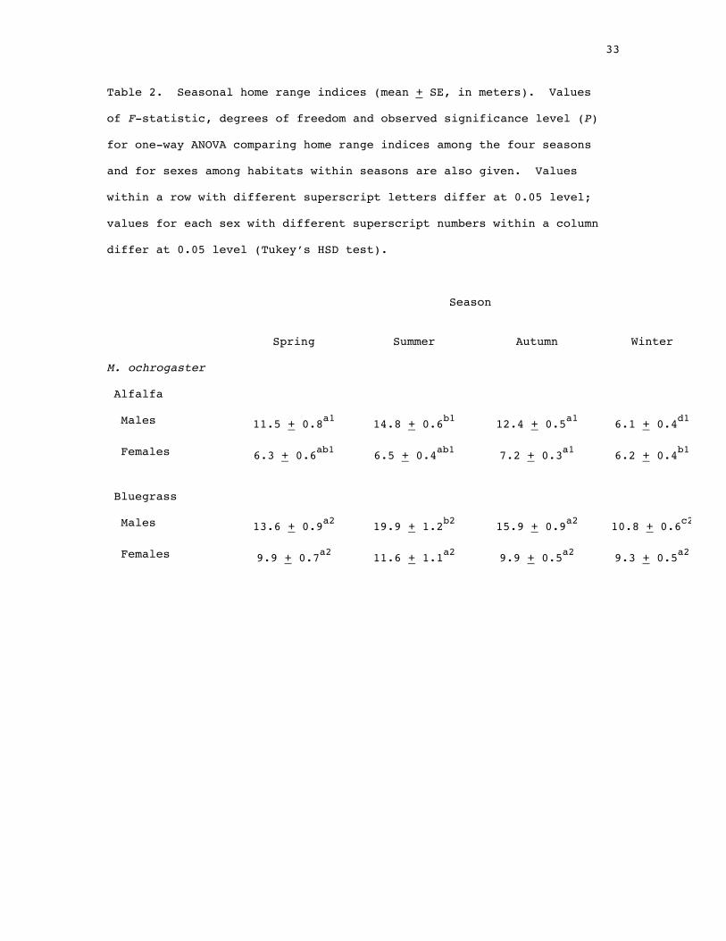
Home range indices of adult males were largest during the summer
and smallest during winter in alfalfa and bluegrass (Table 2). There
was no seasonal difference in adult male home range indices in
tallgrass. The only significant seasonal difference in home range size
of adult females involved larger indices during autumn than winter in
alfalfa. Among habitats, adult male and female indices were
significantly smaller in alfalfa than in bluegrass and tallgrass during
all seasons (Table 2). The only seasonal difference in home range
indices between the latter two habitats was larger adult male home
14
range indices in tallgrass than in bluegrass during winter (Tukey’s
HSD, < 0.05).
Population density and home range indices of adult male and
female M. ochrogaster were not correlated in alfalfa (r = 0.107, N =
213, P = 0.118 and r = 0.099, N = 212, P = 0.153, males and females,
respectively). In bluegrass there was a positive correlation between
population density and male home range indices (r = 0.242, N = 171, P =
0.001) and a negative correlation for female indices (r = -0.231, N =
160, P = 0.003). Home range indices and population density were not
correlated in tallgrass (r = 0.081, N = 90, P = 0.449 and r = 0.051, N
= 74, P = 0.663, males and females, respectively). When home range
indices were grouped into categories of population density, those of
adult males and females in all three habitats were significantly
smaller only during periods of very high population density, > 101/ha
(Table 3).
When compared within habitats over the entire 25 years, body mass
and home range indices of both adult male and female M. ochrogaster
were correlated in alfalfa (r = 0.070, N = 2771, P < 0.001 and r =
0.060, N = 2794, P = 0.001, respectively) and bluegrass (r = 0.074, N =
1938, P = 0.001 and r = 0.053, N = 2018, P = 0.017, respectively).
There was no relationship between body mass and home range indices in
tallgrass (r = 0.013, N = 947, P = 0.686 and r = 0.042, N = 871, P =
0.218, males and females, respectively). When seasonal comparisons
were made of body mass and home range indices within the three
habitats, only five (spring, females in bluegrass; summer, males in
alfalfa and bluegrass; autumn, males in alfalfa and females in
bluegrass) of the 24 possible season x sex x habitat comparisons were
significant.
15
Home range indices of males that were residents at nests of male-
female pairs or communal groups were larger than those of female
residents (9.1 + 1.0 and 5.6 + 0.5, respectively; t = 2.726, d.f. =
286.0, P = 0.007). Home range indices of resident males were smaller
than those of non resident males that wandered within the study sites
(9.1 + 1.0 and 15.8 + 1.8, respectively; t = 3.631, d.f. = 199.7, P <
0.001).
Microtus pennsylvanicus.--Home range indices of all adults
combined and adult females were significantly larger in tallgrass than
in alfalfa or bluegrass (Table 1); home range indices did not differ
between the latter two habitats. Home range indices of adult males,
subadults and juveniles were larger in tallgrass than in bluegrass, but
did not differ between tallgrass and alfalfa. Juvenile home ranges
were significantly smaller in bluegrass than in alfalfa. Adult male
home ranges were larger than those of adult females in all three
habitats (Alfalfa: t = 7.17, d.f. = 465.5, P < 0.001; Bluegrass: t =
698, d.f. = 949.4, P < 0.001; Tallgrass: t = 6.80, d.f. = 1026.4, P <
0.001).
Adult male home ranges were significantly smaller in winter than
during other seasons in alfalfa and bluegrass (Table 2). In tallgrass,
home range indices of adult males were significantly larger during
summer-autumn than winter-spring. The only seasonal difference in home
range indices of adult females within the three habitats was smaller
home ranges during winter than spring in alfalfa.
Although ANOVA analysis indicated there were differences in home
range indices among the three habitats for females during spring, and
males during summer and winter, HSD tests did not indicate which
habitats differed. Pair-wise comparisons of each of the three sets of
samples, using 2-sample t-tests, indicated that home range indices
16
differed between only tallgrass (larger) and bluegrass (smaller).
During winter, male home ranges were smallest in alfalfa, but the
difference from tallgrass only approached significance (t = 1.898, d.f.
= 204, P = 0.059). During autumn, home range indices of both males and
females were larger in tallgrass than in alfalfa or bluegrass. Home
range indices of females during winter were significantly smaller in
alfalfa than in either bluegrass or tallgrass.
Home range indices of male, but not female, M. pennsylvanicus
were positively correlated with population density in alfalfa (r =
0.309, N = 57, P = 0.020 and r = 0.200, N = 62, P = 0.119, males and
females, respectively); however home range indices were negatively
correlated with population density in tallgrass; those of males
approached significance (r = -0.140, N = 177, P = 0.063 and r = -0.194,
N = 163, P = 0.013, males and females, respectively). Home range
indices and population density were not correlated in bluegrass,
although those of females approached significance (r = 0.106, N = 112,
P = 0.265 and r = 0.181, N = 111, P = 0.058, males and females,
respectively). When grouped by categories of population density, there
was no relationship between home range indices and population density
of M. pennsylvanicus in alfalfa. In bluegrass and tallgrass, home
range indices of adult males and females were significantly smaller at
the higher densities; those of males became compressed at lower
densities in the lower food tallgrass than in bluegrass (Table 3).
The only significant relationship between body mass and home
range indices of M. pennsylvanicus within habitats over the 25 years
was for males in tallgrass (r = 0.101, N = 773, P = 0.005). Of the 24
season x sex x habitat comparisons, only female body mass during winter
in bluegrass was significantly negatively related to home range
indices.

17
Interspecific comparisons.--Home range indices of M.
pennsylvanicus (all adults combined, adult males, adult females) were
significantly larger (P <0.001) than those of M. ochrogaster in all
three habitats (Table 1). The differences were much more pronounced in
alfalfa than in bluegrass or tallgrass. Sample sizes of M.
pennsylvanicus were too small for interspecific comparisons of subadult
and juvenile home ranges.
Male M. pennsylvanicus home range indices in alfalfa were larger
than those of wandering male M. ochrogaster (20.3 + 1.3 and 15.8 + 1.8,
respectively; t = 3.135, d.f. = 147.9, P = 0.002).
Response to supplemental feeding.--There were no differences in
home range indices of adult males or females of either species in
supplementally fed and control bluegrass sites (Table 4). There also
were no differences in home range indices of adult male and female M.
ochrogaster in supplementally fed and control tallgrass sites. Home
ranges of adult male and female M. pennsylvanicus, however, were
significantly smaller in supplementally fed than in control tallgrass
sites (Table 4).
Seasonal sample sizes (adult males and females, combined) were
sufficient for comparison of home ranges in supplementally fed and
control sites during the winter only in tallgrass. There was no
difference in home range indices of M. ochrogaster (12.4 + 1.9 and 13.
2 + 1.8, supplementally fed and control respectively; t = 0.271, d.f. =
85, P = 0.787). Indices for M. pennsylvanicus during winter were
significantly smaller in the supplementally fed tallgrass site than the
control (8.7 + 0.9 and 12.9 + 1.4, respectively; t = 2.588, d.f. =
130.3, P = 0.011).
Interspecific interactions.--Overall, presence of one species had
little impact on home range indices of the other species. There was no
18
difference in the home range indices of adult male and female M.
ochrogaster when alone and when M. pennsylvanicus was present at
population densities above the mean density for bluegrass (14/ha) in
the control site (male indices: 9.8 + 1.0 and 10.4 + 1.6 when alone and
in the presence of M. pennsylvanicus, respectively, t = 0.682, d.f. =
214, P = 0.496; females: 9.1 + 1.0 and 7.9 + 0.8, respectively; t =
0.861, d.f. = 253, P = 0.390). When home range indices were estimated
for adult males and females of each species in bluegrass over the
entire 25-year period, relative to periods when population density of
the other species was below or above the mean for bluegrass, the only
significant difference concerned larger indices of female M.
ochrogaster when densities of M. pennsylvanicus were above mean
densities (males: 15.2 + 0.6 and 15.7 + 1.5; t = 0.415, d.f. = 1227, P
= 0.678; females: 10.7 + 0.5 and 12.4 + 1.1; t = 2.747, d.f. = 405.4, P
= 0.006; below and above the mean, respectively). There was no
difference in home range indices of either male or female M.
pennsylvanicus when densities of M. ochrogaster were below or above the
mean density for bluegrass (males: 17.6 + 0.8 and 18.7 + 1.4; t =
1.066, d.f. = 492, P = 0.287; females: 11.0 + 0.5 and 14.5 + 1.3; t =
1.680, d.f. = 613, P = 0.093).
Discussion
In this study, mean home range indices for Microtus ochrogaster
among the three habitats suggested home range size was inversely
related to food availability. For all sex and age categories, home
range indices were smallest in alfalfa (high food habitat),
intermediate in bluegrass (intermediate food habitat) and largest in
tallgrass (low food habitat). Seasonal comparisons of home range
indices of M. ochrogaster among the three habitats also reflected the
19
influence of food availability. Home range indices of adult male and
female M. ochrogaster were consistently smaller in alfalfa than in
bluegrass and tallgrass during all four seasons. Further, indices of
adult male home ranges during winter were larger in tallgrass than in
bluegrass.
Within-habitat seasonal variation in home range indices of M.
ochrogaster did not reflect presumed changes in food availability.
Food availability was presumed to be lesser during winter than other
seasons in all three habitats and greater in alfalfa during winter than
in bluegrass or tallgrass (Getz et al. In Review a). Home range
indices of adult males, on the other hand, were significantly smaller
during winter than other seasons in both alfalfa and bluegrass and
there was no seasonal difference in home range indices of males in
tallgrass. Home range indices of females did not differ seasonally in
any of the three habitats.
The association between food availability and home range indices
among the three habitats was less obvious for M. pennsylvanicus than
for M. ochrogaster. Only total adult and adult female home range
indices were significantly larger in the low food tallgrass habitat
than in high food alfalfa and intermediate food bluegrass. Further,
there was no difference between home range indices of adults in
intermediate food bluegrass and high food alfalfa. In addition, there
were few among-habitat seasonal differences in home range indices of M.
pennsylvanicus with respect to presumed food availability. As for M.
ochrogaster, within-habitat seasonal differences in home range indices
of M. pennsylvanicus were inconsistent in respect to food availability.
Variation in home range indices of M. ochrogaster in response to
supplemental feeding did not support our predictions. There was no

20
difference in home range indices of adult males and females in
supplementally fed and control sites in bluegrass or tallgrass.
Home range indices of both sexes of M. pennsylvanicus were smaller in
supplementally fed than in control tallgrass but did not differ between
supplementally fed and control bluegrass sites. When compared
seasonally, home range indices of M. pennsylvanicus in the
supplementally fed tallgrass site were smaller than those in the
control site during all seasons except autumn. However, only the
differences during spring were statistically significant. These
results suggest that while the abundance of food resources generally
may result in smaller home range sizes in M. pennsylvanicus, effects of
food availability on home range sizes may vary seasonally.
The results from the supplemental feeding study are consistent
with demographic responses of the two species to the addition of food
to bluegrass and tallgrass sites. Population densities of M.
ochrogaster did not change in response to supplemental feeding in
bluegrass and tallgrass. M. pennsylvanicus displayed higher population
densities in supplementally fed than control tallgrass, but not in
bluegrass sites (Getz et al. 1987, In Review b).
In the manipulative studies, presence of the other species, even
at high densities, did not result in differences in home ranges of
either M. ochrogaster or M. pennsylvanicus. This provides additional
evidence that there was little relationship between home range size and
food availability. Since the two species feed on the same plants, high
densities of one species should effectively reduce food availability
for the other. Accordingly, one would expect home ranges to be larger,
if there was no interspecific social interaction restricting movements
of the two species as food availability per individual became less. If
interspecific interactions restricted access of individuals of one or

21
both species to food, smaller home ranges would be displayed by one or
both species. However, home range sizes of neither species differed in
the presence of the other species.
Although home ranges of M. ochrogaster were positively associated
with body mass, such a response did not appear related to energy
requirements. The positive responses were observed in the higher food
habitats, alfalfa and bluegrass, but not in low food tallgrass.
Neither did the mating system appear to be involved, as was observed in
Dicrostonyx groenlandicus (Schmidt et al. 2002).
Our results regarding interactions between home range size and
presumed food availability agree only very generally with those of
Meserve (1971), Taitt and Krebs (1981), Boutin (1990), Jones (1990),
and Fortier and Tamarin (1998), who found home ranges to be smaller
where food availability is greater. Our results also do not agree
entirely with those of Swihart and Slade (1989), Abramsky and Tracy
(1980), Desy et al. (1990), Fortier et al. (2001), in which home range
sizes were found to be either the same or smaller in low food sites in
comparison to where food was more abundant.
Abramsky and Tracy (1980), Gaines and Johnson (1982), Ostfeld and
Canham (1995), and Fortier and Tamarin (1998) have shown home ranges to
be compressed as population density and competition for resources
increased. Our results indicated such a relationship either was
expressed only at very high densities (M. ochrogaster) or was not
consistent with predicted interactions with food availability (M.
pennsylvanicus). There was no direct interaction between population
density and food availability in relation to home range size of M.
ochrogaster. Home ranges of both adult males and females became
significantly smaller only at population densities > 101/ha,
irrespective of food availability, suggesting that only very high
22
population densities result in compression of home ranges. Similarly,
variation in home range sizes of M. pennsylvanicus did not display an
interaction between population density and food availability. Indices
of M. pennsylvanicus became compressed at lower population densities
where food was presumed to be less available, the opposite of what one
would anticipate if food were a major determinant of home range size.
We conclude elsewhere that among-habitat differences in
demography of M. ochrogaster and M. pennsylvanicus result from
differences in survival related to vegetative cover, not food
availability (Getz et al. In Review a). On first appraisal, our
analyses of home range indices appear to agree with these conclusions.
However, seasonal/habitat differences in home range indices are not
entirely consistent with conclusions regarding influence of cover.
Anderson (1986) and Desy et al. (1990) found home ranges of some
species of arvicoline rodents to be smaller in sites where the risk of
predation is greater, i.e., habitats with sparse cover. Our data
suggest a similar response to risk of predation, but the effect is
complicated by variation in food availability. Cover was less
throughout the year in alfalfa than in either bluegrass or tallgrass
and within alfalfa, less during the winter than other seasons; there
was little seasonal difference in cover in bluegrass and tallgrass
(Getz et al. In Review a). Although lower during winter than other
seasons within each of the three habitats, food availability during the
winter was greater in alfalfa than in bluegrass or tallgrass.
Overall home range indices of both species varied as would be
expected if cover/predation risk were mainly involved, i.e., smaller in
alfalfa than in bluegrass and tallgrass. Home range indices of males
of both M. ochrogaster and M. pennsylvanicus were smaller during the
winter than other seasons in alfalfa and bluegrass, but not in
23
tallgrass. This suggests food may be a more important factor than
cover in determining home ranges size. On the other hand, home range
indices of adult males of both species were smaller in alfalfa during
winter when food was comparatively low, than during other seasons, when
food was more abundant. This suggests a response to predator risk.
There was, however, no difference in home range indices of female M.
ochrogaster and only a tendency for smaller indices of female M.
pennsylvanicus during winter in alfalfa than in other seasons. This
suggests that, if predation risk were a factor in home range sizes,
only males display such a response. Desy et al. (1990) found no such
sex differences in relation to prey risk of M. ochrogaster.
We found that adult male home range indices of both M.
ochrogaster (monogamous) and M. pennsylvanicus (promiscuous) were
greater than those of adult females. Further, males of male-female
pairs and communal groups of M. ochrogaster had larger home range
indices than did resident females. Resient males make brief forays out
of the shared home range (Hofmann et al. 1984; Getz et al. 1986;
McGuire and Getz 1998; McGuire et al. 1990), and this may contribute to
their larger home range indices. On the other hand, resident male M.
ochrogaster had significantly smaller home range indices than did
wandering males, suggesting that the social status of males influences
their home range size. Thus, our results agree those of Swihart and
Slade (1989) who found male M. ochrogaster home ranges to be larger
than those of females. Our results agree only partially with those of
Gaulin and Fitzgerald (1988) who found home range sizes did not differ
between male and female M. ochrogaster. That our data were from a high
food habitat, while those of the latter two studies were from lower
food situations, may confound comparisons.
24
Home range indices for M. pennsylvanicus were larger than those
of M. ochrogaster. Larger body mass of M. pennsylvanicus (Getz et al.
In Review a) and presumed greater food requirements may, in part, be
involved. One would expect the same relative differences between home
range indices of the two species, irrespective of food level, if home
range sizes were influenced primarily by food availability. However,
differences were greatest in the high food alfalfa habitat, where the
home ranges of the two species would be expected to be more similar
than where food was less abundant.
It thus appears variation in home range size is complexly
involved in demography of M. ochrogaster and M. pennsylvanicus, and
that such interactions vary with species and habitat. Under some
circumstances, increased population density may result in smaller home
ranges and less food availability to individuals. Under other
conditions, however, home ranges are not compressed, except at very
high densities, and are not related to food availability.
In conclusion, we found only partial support for our original
predictions: (1) there was only a general correlation between food
availability and home range sizes, and such agreement was not
consistent with seasonal variation in food availability; (2) home range
size was compressed only at relatively high densities; (3) there was no
effect of interspecific interactions on home range sizes of either
species; (4) while risk of predation may have influenced home range
size, the effect was confounded by food availability; and (5) there was
little correlation between home range sizes of M. ochrogaster and M.
pennsylvanicus that could be explained by species differences in mating
system.
Acknowledgements

25
The study was supported in part by grants NSF DEB 78-25864 and
NIH HD 09328 to LLG and by the University of Illinois School of Life
Sciences and Graduate College Research Board. We thank the following
individuals for their assistance with the field work: L. Verner, R.
Cole, B. Klatt, R. Lindroth, D. Tazik, P. Mankin, T. Pizzuto, M.
Snarski, S. Buck, K. Gubista, S. Vanthernout, M. Schmierbach, D.
Avalos, L. Schiller, J. Edgington, B. Frase, and the 1,063
undergraduate “mouseketeers” without whose extra hands in the field the
study would not have been possible. C. Haun, M. Thompson and M.
Snarski entered the data sets into the computer.
Literature cited
Abramsky, Z., and C. R. Tracy. 1980. Relation between home range size
and regulation of population size in Microtus ochrogaster. Oikos
34:347-355.
Akbar, Z., and M. L. Gorman. 1993. The effect of supplementary
feeding upon sizes of the home ranges of wood mice Apodemus
sylvaticus living on a system of maritime sand dunes. Journal of
Zoology, London 231:33-237.
Anderson, P. K. 1986. Foraging range in mice and voles: the role of
risk. Canadian Journal of Zoology 64:2645-2653.
Boutin, S. 1990. Food supplementation experiments with terrestrial
vertebrates: pattern, problems and future. Canadian Journal of
Zoology 68:203-220.
Burt, W. H. 1940. Territorial behavior and populations of some small
mammals in southern Michigan. University of Michigan Museum of
Zoology Miscellaneous Publications 45:1-58.
26
Cole, F. R., and G. O. Batzli. 1979. Nutrition and populations of the
prairie vole, Microtus ochrogaster, in Central Illinois. Journal
of Animal Ecology 48:455-470.
Desy, E. A., G. O. Batzli, and J. Liu. 1990. Effects of food and
predation on behavior of prairie voles: a field experiment.
Oikos 58:159-168.
Efford, M. 1992. Comment-revised estimates of the bias in minimum
number alive estimator. Canadian Journal of Zoology 70:628-631.
Fortier, G. M., and R. H. Tamarin. 1998. Movement of meadow voles in
response to food and density manipulations: a test of the food-
defense and pup-defense hypotheses. Journal of Mammalogy 79:337-
345.
Fortier, G. M., M. A. Osmon, M. Roach, and K. Clay. 2001. Are female
voles food limited? Effects of endophyte-infected fescue on home
range size in female prairie voles (Microtus ochrogaster). The
American Midland Naturalist 146:63-71.
Gaines, M. S., and M. L. Johnson. 1982. Home range size and
population dynamics in the prairie vole, Microtus ochrogaster.
Oikos 39:63-70.
Gaulin, S. J., C. and R. W. Fitzgerald. 1988. Home-range size as a
predictor of mating systems in Microtus. Journal of Mammalogy
69:311-319.
Getz, L. L., F. R. Cole, L. Verner, J. E. Hofmann, and D. Avalos.
1979. Comparisons of population demography of Microtus
ochrogaster and M. pennsylvanicus. Acta Theriologica 24:319-349.
Getz, L. L., J. E. Hofmann, and L. Jike. l986. Relationship between social
organization, mating system and habitats of microtine rodents. Acta
Theriologica Sinica 6:273-285.

27
Getz, L. L., J. E. Hofmann, B. J. Klatt, L. Verner, F. R. Cole, and R.
L. Lindroth. 1987. Fourteen years of population fluctuations of
Microtus ochrogaster and M. pennsylvanicus in east central
Illinois. Canadian Journal of Zoology 65:1317-1325.
Getz, L. L.,B. McGuire, J. E. Hofmann, T. Pizzuto, and B. Frase.
1993. Social organization of the prairie vole (Microtus
ochrogaster). Journal of Mammalogy 74:44-58.
Getz, L. L., J. Hofmann, B. McGuire, and T. Dolan III. 2001. Twenty-five
years of population fluctuations of Microtus ochrogaster and M.
pennsylvanicus in three habitats in east-central Illinois. Journal of
Mammalogy 82:22-34.
Getz, L. L., J. E. Hofmann, B. McGuire, and M. K. Oli. In Review a.
Habitat-specific demography of sympatric vole populations. Canadian
Journal of Zoology.
Getz, L. L., J. E. Hofmann, B. McGuire, and M. K. Oli. In Review b.
Dynamics of sympatric vole populations: influence of food resources and
interspecific competition. Journal of Animal Ecology
Hayne, D. W. 1949. Calculation of size of home range. Journal of Mammalogy
30:1-18.
Hayne, D. W. 1950. Apparent home range of Microtus in relation to distance
between traps. Journal of Mammalogy 31:26-39.
Hofmann, J. E., L. L. Getz, and L. Gavish. l984. Home range overlap and
nest cohabitation of male and female prairie voles. The American
Midland Naturalist ll2:3l4-3l9.
Hubbs, A. H., and R. Boonstra. 1998. Effects of food and predators on the
home-range sizes of Arctic ground squirrels (Spermophilus parryii).
Canadian Journal of Zoology 76:592-596
28
Ims, R. A. 1987. Responses in spatial organization and behaviour to
manipulations of food resources in the vole Clethrionomys rufocanus.
Journal of Animal Ecology 56:585-596.
Jones, E. N. 1990. Effect of forage availability on home range size and
population density of Microtus pennsylvanicus. Journal of Mammalogy
71: 382-389.
Jones, E. N., and L. J. Sherman. 1983. A comparison of meadow vole home
ranges derived from grid trapping and radiotelemetry. Journal of
Wildlife Management 47:558-561.
Krebs, C. J. 1966. Demographic changes in fluctuating populations of
Microtus californicus. Ecological Monographs 36: 239-273.
Krohne, D. T. 1986. Sensitivity of home range estimates to sample
sizes in Peromyscus. Canadian Journal of Zoology 64:2873-2875.
Lacki, M. J., M. J. Gregory, and P, K. Williams. 1984. Spatial
response of an eastern chipmunk population to supplemental food.
The American Midland Naturalist 111:114-116.
Lindroth, R. L., and G. O. Batzli. 1984. Food habits of the meadow
vole (Microtus pennsylvanicus) in bluegrass and prairie habitats.
Journal of Mammalogy 65:600-606.
Mares, M. A., and T. E. Lacher, Jr. 1987. Social spacing in small
mammals; patterns of individual varation. American Zoologist
27:293-306.
Mares, M. A., T. E. Lacher Jr., M. W. Willig, N. A. Bitar, R. Adams,
and D. Tazik. 1982. An experimental analysis of social spacing
in Tamias striatus. Ecology 63:267-273.
McGuire, B., and L. L. Getz. 1998. The nature and frequency of social
interactions among free-living prairie voles (Microtus ochrogaster).
Behavioural Ecology and Sociobiology 43:271-279.

29
McGuire, B., T. Pizzuto, and L. L. Getz. 1990. Potential for social
interaction in a natural population of prairie voles (Microtus
ochrogaster). Canadian Journal of Zoology 68:391-398.
Meserve, P. L. 1971. Population ecology of the prairie vole, Microtus
ochrogaster, in the western mixed prairie of Nebraska. The
American Midland Naturalist 86:417-433.
Oli, M. K., H. A. Jacobson, and B. D. Leopold. 2002. Pattern of space
use by female black bears in the White River National Wildlife
Refuge, Arkansas, USA. Journal for Nature Conservation 10:87-93.
Ostfeld, R. S., and C. D. Canham. 1995. Density-dependent processes
in meadow voles: an experimental approach. Ecology 76:521-532.
Pollock, K. H., Nichols, J. D., Brownie, C., and Hines, J.E. 1990.
Statistical inference for capture-recapture experiments.
Wildlife Monogrographs 107:1-97.
Ribble, D. O., A. E. Wurtz, and E. K. McConnell. 2002. A comparison
of home ranges of two species of Peromyscus using trapping and
radiotelemetry data. Journal of Mammalogy 83:260-266.
Rodd, F. H., and R. Boonstra. 984. The spring decline in the meadow
vole, Microtus pennsylvanicus: the effect of density. Canadian
Journal of Zoology 62:1464-1473.
Schmidt, N. M., T. B Berg, and T. S. Jensen. 2002. The influence of
body mass on daily movement patterns and home ranges of the
collared lemming (Dicrostonyx groenlandicus). Canadian Journal
of Zoology 80:64-69.
Slade, N. A., and R. K Swihart. 1983. Home range indices for the
hispid cotton rat (Sigmadon hispidus) in northeastern Kansas.
Journal of Mammalogy 64:580-590.
30
Slade, N. A., L. A. Russell, and T. J. Doonan. 1997. The impact of
supplemental food on movements of prairie voles (Microtus
ochrogaster). Journal of Mammalogy 78:1149-1155.
Slade, N. A., and L. A. Russell. 1998. Distances as indices to
movements and home-range size from trapping records of small
mammals. Journal of Mammalogy 79:346-351.
SPSS, Inc. 2001. SPSS 10.0.7 for Macintosh. Chicago, Illinois
Swihart, R. K., and N. A. Slade. 1989. Differences in home-range size
between sexes of Microtus ochrogaster. Journal of Mammalogy
70:816-820.
Taitt, M. J., and C. J. Krebs. 1981. The effects of extra food on
small rodent populations: II. Voles (Microtus townsendii).
Journal of Animal Ecology 50:125-137.
Taitt, M. J., and C. J. Krebs. 1985. Population dynamics and cycles.
Pp. 567-620 in Biology of New World Microtus (R. H. Tamarin,
ed.). Special Publication, American Society of Mammalogists 8:1-
893.
Vincent, J. P., E. Bideau, A. J. M. Hewison, and J. M. Angibault. 1995.
The influence of increasing density on body weight, kid
production, home range and winter grouping in roe deer (Capreolus
capreolus). Journal of Zoology (London) 236:371-382.
Wolff, J. O. 1985. The effects of density, food, and interspecific
interference on home range size in Peromyscus leucopus and
Peromyscus maniculatus. Canadian Journal of Zoology 63:2657-
2662.
Zar, J. H. 1999. Biostatistical analysis. 4th Ed. Prentice Hall.
Upper Saddle River, New Jersey.

31
Table 1. Mean home range indices (mean + SE, in meters) by
habitat. Values of F-statistic, degrees of freedom, and
observed significance level (P) for one-way ANOVA comparing
home range indices among the three habitats are also given.
Values within a row with different superscript letters differ
significantly at 0.05 level (Tukey’s HSD test). Independent-
sample t-tests were used to compare paired means of total
adult, adult male and adult female M. ochrogaster and M.
pennsylvanicus; paired values in each column with different
superscript numbers differ at 0.001 level.
Habitat F; df
Alfalfa Bluegrass Tallgrass
M. ochrogaster
Total adults 8.9 + 0.2a1 13.2 + 0.4b1 15.5 + 0.6c1 158.383; 2,8689 <0.001
Adult males 11.1 + 0.3a1 15.3 + 0.6b1 17.5 + 0.9c1 62.5039; 2,4351 <0.001
Adult females 6.7 + 0.2a1 11.2 + 0.5b1 13.3 + 0.8c1 108.4464; 2,4335 <0.001
Subadult 7.7 + 0.6a 12.2 + 0.7b 17.7 + 1.9c 49.4942; 2,1616 <0.001
Juveniles 5.2 + 0.3a 8.3 + 0.8b 13.9 + 1.4c 34.1321; 2,991 <0.001

32
Table 1 (Cont.)
M. pennsylvanicus
Total adults 15.6 + 0.7a2 14.4 + 0.4a2 18.6 + 0.6b2 6.053; 2,2602 <0.001
Adult males 20.2 + 1.3ab2 17.7 + 0.8b2 22.8 + 1.0a2 6.9803; 2,1211 <0.001
Adult females 11.8 + 0.8a2 11.8 + 0.4a2 14.4 + 0.5b2 19.1112; 2,1388 <0.001
Subadult 14.2 + 1.8ab 10.7 + 0.7b 14.2 + 0.6a 12.8429; 2,667 <0.001
Juveniles 14.1 + 2.6a 8.1 + 0.8b 13.9 + 1.4a 8.7809; 2,194 <0.001
33
Table 2. Seasonal home range indices (mean + SE, in meters). Values
of F-statistic, degrees of freedom and observed significance level (P)
for one-way ANOVA comparing home range indices among the four seasons
and for sexes among habitats within seasons are also given. Values
within a row with different superscript letters differ at 0.05 level;
values for each sex with different superscript numbers within a column
differ at 0.05 level (Tukey’s HSD test).
Season F; df
Spring Summer Autumn Winter
M. ochrogaster
Alfalfa
Males 11.5 + 0.8a1 14.8 + 0.6b1 12.4 + 0.5a1 6.1 + 0.4d1 68.5839; 3,2768
Females 6.3 + 0.6ab1 6.5 + 0.4ab1 7.2 + 0.3a1 6.2 + 0.4b1 3.0212; 3,2791
Bluegrass
Males 13.6 + 0.9a2 19.9 + 1.2b2 15.9 + 0.9a2 10.8 + 0.6c2 25.051; 3,1935
Females 9.9 + 0.7a2 11.6 + 1.1a2 9.9 + 0.5a2 9.3 + 0.5a2 1.6710; 3,2015

34
Table 2 (Cont.)
Tallgrass
Males 16.0 + 1.0a2 15.5 + 1.1a2 15.1 + 1.0a2 13.0 + 0.8a3 2.5680; 3,94
Females 10.7+ 0.9a2 11.0 + 0.8a2 11.2 + 0.8a2 11.4 + 1.0a2 0.2617; 3,868
Males; F, df 15.164, 2,974 4.186, 2,1101 16.797, 2,1865 51.270, 2,1708
P < 0.001 0.015 < 0.001 < 0.001
Females; F, df 16.435, 2,820 22.717, 2,1203 35.571, 2,2204 25.788, 2,1447
P < 0.001 < 0.001 < 0.001 < 0.001
M. pennsylvanicus
Alfalfa
Males 22.6 + 2.5a1 19.4 + 2.4a1 21.6 + 2.1a1 9.6 + 1.5b12 3.796; 3,221
Females 17.0 + 2.6a12 11.5 + 1.7ab1 11.4 + 1.1ab1 7.6 + 1.1b1 3.6888; 3,261

35
Table 2 (Cont.)
Bluegrass
Males 19.8 + 1.0a1 18.3 + 1.3a1 18.3 + 1.3a1 14.2 + 2.0b1 10.925; 3,678
Females 12.4 + 0.8a1 11.8 + 1.1a1 12.9 + 0.8a1 12.5 + 1.3a12 0.6497; 3,850
Tallgrass
Males 18.6 + 0.9a1 22.5 + 1.5b1 30.1 + 2.2b2 18.0 + 1.3a2 12.8959; 3,770
Females 13.2 + 0.7a2 13.3 + 1.1a1 16.2 + 1.0a2 15.2 + 1.2a2 1.3996; 3,563
Males; F, df 1.383, 2,614 3.698, 2,315 6.924, 2,398 7.024, 2,306
P 0.252 0.026 0.001 0.001
Females; F, df 3.573, 2,486 1.496, 2,270 8.106, 2,595 6.147, 2,323
P 0.029 0.226 < 0.001 0.002

36
Table 3. Home range indices (mean + SE, in meters) in relation
to population densities. Values of F-statistic, degrees of
freedom and observed significance level (P) for one-way ANOVA
comparing home range indices among the population density
categories. Values within a row with different superscripts
differ significantly at 0.05 level.
Population density F; df
1-25/ha 26-50/ha 51-100/ha >101/ha
M. ochrogaster
Alfalfa
Males 17.2 + 1.1a 14.7 + 1.3a 13.2 + 0.6a 8.0 + 0.4b 71.788; 3,2750 <0.0001
Females 8.6 + 0.8a 8.3 + 0.9a 7.4 + 0.4a 5.6 + 0.2b 45.573; 3,3045 <0.0001
Bluegrass
Males 14.4 + 0.7a 15.6 + 0.8a 16.0 + 1.0a 11.2 + 0.7b 10.053; 3,1918 <0.0001
Females 10.5 + 0.7a 11.9 + 0.9a 10.6 + 0.6a 7.5 + 0.4b 10.599; 3,1998 <0.0001

37
Table 3 (Cont.)
Tallgrass
Males 18.7 + 1.2a 14.8 + 1.1a 16.6 + 1.1a 10.4 + 0.7b 10.914; 3,877 <0.0001
Females 13.6 + 1.0a 11.6 + 1.2a 12.0 + 0.9a 8.7 + 0.7b 7.980; 3,810 <0.0001
M. pennsylvanicus
Alfalfa
Males 17.5 + 22.4a 26.0 + 3.8a 17.8 + 2.0a 21.7 + 2.3a 1.971; 3,214 0.1193
Females 12.7 + 2.3a 13.1 + 2.5a 11.7 + 1.1a 11.1 + 1.5a 0.615; 3,265 0.183

38
Table 3 (Cont.)
Bluegrass
Males 21.6 + 1.9a 24.3 + 2.2a 18.4 + 0.9a 15.0 + 0.9b 5.982; 3,667 0.0005
Females 14.8 + 1.5a 14.9 + 1.4a 11.4 + 0.6b 10.6 + 0.8b 4.511; 3,836 0.0038
Tallgrass
Males 28.7 + 2.0a 20.5 + 0.9b 13.6 + 0.6c 14.5 + 0.9c 215.086; 3,944 <0.0001
Females 16.8 + 2.0a 14.9 + 0.6a 11.0 + 0.6b 9.1 + 0.6b 17.083; 3,785 <0.0001

39
Table 4. Home range indices (mean + SE, in meters) in supplementally fed and
control sites. Values of t statistic, degrees of freedom and observed significance
level (P) are given.
Study site t; df P
Supplementally fed Control
M. ochrogaster
Bluegrass
Males 18.4 + 2.0 14.0 + 1.1 1.27, 235 0.207
Females 9.0 + 1.7 9.9 + 0.9 1.46, 189 0.146
Tallgrass
Males 14.0 + 1.3 18.7 + 2.0 1.74, 281 0.096
Females 11.4 + 1.0 12.9 + 2.0 0.303; 173 0.763
M. pennsylvanicus
Bluegrass
Males 17.7 + 1.4 15.9 + 0.9 1.33, 341 0.183
Females 11.2 + 1.3 9.9 + 0.5 0.28, 356 0.782
Tallgrass
Males 13.2 + 0.6 16.4 + 0.7 3.17, 566 0.002
Females 10.2 + 0.5 12.6 + 0.6 3.32, 406.8 0.001
Top Related