Zhu Qualifier Solutions

Draft version June 20, 2012Preprint typeset using LATEX style emulateapj v. 5/2/11

QUALIFIER EXAM SOLUTIONS

Chenchong Zhu(Dated: June 20, 2012)

Contents

1. Cosmology (Early Universe, CMB, Large-Scale Structure) 71.1. A Very Brief Primer on Cosmology 7

1.1.1. The FLRW Universe 71.1.2. The Fluid and Acceleration Equations 71.1.3. Equations of State 81.1.4. History of Expansion 81.1.5. Distance and Size Measurements 8

1.2. Question 1 91.2.1. Couldn’t photons have decoupled from baryons before recombination? 101.2.2. What is the last scattering surface? 11

1.3. Question 2 111.4. Question 3 12

1.4.1. How do baryon and photon density perturbations grow? 131.4.2. How does an individual density perturbation grow? 141.4.3. What is violent relaxation? 141.4.4. What are top-down and bottom-up growth? 151.4.5. How can the power spectrum be observed? 151.4.6. How can the power spectrum constrain cosmological parameters? 151.4.7. How can we determine the dark matter mass function from perturbation analysis? 15

1.5. Question 4 161.5.1. What is Olbers’s Paradox? 161.5.2. Are there Big Bang-less cosmologies? 16


1.7.1. How can we possibly see galaxies that are moving away from us at superluminal speeds? 181.7.2. Why can’t we explain the Hubble flow through the physical motion of galaxies through space? 191.7.3. Can galaxies with recession velocities v > c slow down until v < c? 19

1.8. Question 7 191.8.1. How does nucleosythesis scale with cosmological parameters? 201.8.2. How do we determine primordial densities if D is easily destroyed in stars? 201.8.3. Why is there more matter than antimatter? 201.8.4. What are WIMPs? 20

1.9. Question 8 201.9.1. Describe systematic errors. 211.9.2. Describe alternate explanations to the SNe luminosity distance data, and why they can be ruled

out? 221.9.3. Can SNe II be used as standard candles? 23

1.10. Question 9 231.10.1. What is the fate of the universe, given some set of Ωs? 231.10.2. How do we determine, observationally, the age of the universe? 241.10.3. Is Λ caused by vacuum energy? 25

1.11. Question 10 251.11.1. What are the consequences of these numbers on the nature of the universe? 261.11.2. How do we determine Ωr from the CMB? 261.11.3. How are other values empirically determined? 261.11.4. What are the six numbers that need to be specified to uniquely identify a ΛCDM universe? 271.11.5. Why is h often included in cosmological variables? 27

1.12. Question 11 271.12.1. What are the possible fates the universe? 28

1.13. Question 12 29

[email protected]

mailto:[email protected]

2

1.13.1. How does the CMB power spectrum support the inflation picture? 311.13.2. Derive the horizon size at recombination. 311.13.3. Why is the CMB a perfect blackbody? 311.13.4. How is the CMB measured? 321.13.5. Why did people use to think CMB anisotropy would be much larger than it is currently known to

be? 321.13.6. What is the use of CMB polarization? 32

1.14. Question 13 321.14.1. Why is BAO often used in conjunction with CMB? 351.14.2. What is the BAO equivalent of higher-l CMB peaks? 35

1.15. Question 14 351.15.1. How is weak lensing measured? 361.15.2. Can strong lensing be used to determine cosmological parameters? 36

1.16. Question 15 361.16.1. What caused inflation? 371.16.2. How does inflation affect the large scale structure of the universe? 371.16.3. Is inflation the only way to explain the three observations above? 37

1.17. Question 16 371.17.1. Is the anthropic principle a scientifically or logically valid argument? 38

1.18. Question 17 381.18.1. Describe galaxy surveys. 391.18.2. What about three or higher point correlation functions? 39


1.20.1. What about He reionization? 41

2. Extragalactic Astronomy (Galaxies and Galaxy Evolution, Phenomenology) 432.1. Question 1 43

2.1.1. What does the Hubble sequence miss? 442.1.2. What is the Tully-Fisher relationship? 452.1.3. What is the fundamental plane? 452.1.4. What other criteria could be used for galaxy classification? 45

2.2. Question 2 452.2.1. Why can’t we simply use the inner 10 kpc data derived from 21-cm line emission and a model of

the halo to determine the mass of the halo? 462.2.2. How is the total mass of an elliptical galaxy determined? 46

2.3. Question 3 472.3.1. Is He and metals ionized? Is any component of the IGM neutral? 472.3.2. What are the properties of these neutral H clouds? Can they form galaxies? 48


2.5.1. How are SMBHs formed? 522.5.2. What correlations are there between the properties of the SMBH and the host galaxy? 52


2.7.1. What determines the emission spectrum of an AGN? 542.7.2. Are there backgrounds at other wavelengths? 54

2.8. Question 8 542.8.1. What are cold flows? 552.8.2. What is feedback? 552.8.3. What is downsizing? 56

2.9. Question 9 562.9.1. What are cooling flows? 57


2.11.1. Describe population synthesis. 602.11.2. What do the spectra of real galaxies look like? 60

2.12. Question 12 602.12.1. What have we learned about high-z galaxies from LBGs? 622.12.2. Are there other “breaks” that could be used to detect galaxies? 622.12.3. Can we find Lyman-break galaxies at low redshifts? 62

2.13. Question 13 622.13.1. What is the cause of the various emission features of AGN? 64

2.14. Question 14 64

3

2.14.1. Are there non-EM backgrounds? 662.15. Question 15 66

2.15.1. Where are most AGN located? 692.15.2. What evidence is there that AGN are powered by supermassive black holes? 69

2.16. Question 16 692.16.1. How are high-z cluster found? 71


2.18.1. What are SZ surveys conducted with? 742.18.2. What is the kinematic SZ effect? 74

3. Galactic Astronomy (Includes Star Formation/ISM) 753.1. Question 1 75

3.1.1. What is the IMF useful for? 753.1.2. Is there a universal IMF? 753.1.3. Why are the lower and upper limits of the IMF poorly understood compared to that of the

middle (several M stars)? What constraints are there? 763.1.4. What’s the difference between a field and stellar cluster IMF? 773.1.5. How do you determine an a present-day mass function (PDMF) from an IMF? 77

3.2. Question 2 773.2.1. What Orbits are Allowed in an Axisymmetric Potential? 783.2.2. How did each population of stars gain their particular orbit? 783.2.3. Orbits in Elliptical Galaxies 793.2.4. What are the different populations in the galaxy, and what are their ages and metallicities? 803.2.5. What is the spheroid composed of (globular clusters?)? 80

3.3. Question 3 803.3.1. What errors are in your analysis? 803.3.2. Can you give some real statistics for SNe Ia? 81

3.4. Question 4 813.4.1. What stars are collisional? 823.4.2. Gas is collisional. Why? 82

3.5. Question 5/6 823.5.1. How does H2 form? 823.5.2. Why is H2 necessary for star formation? 833.5.3. How do Population III stars form? 83

3.6. Question 7 843.6.1. What observational differences are there between GCs and dSphs? 843.6.2. What is a Galaxy? 84

3.7. Question 8 853.7.1. How does velocity dispersion increase over time? 853.7.2. Why is the mean [Fe/H] not -∞ at the birth of the MW? 86


3.9.1. Given a cross-section, how would you calculate the amount of extinction? 903.9.2. What percentage of the light is absorbed (rather than scattered) by the light? 903.9.3. Why is dust scattering polarized? 903.9.4. What is the grain distribution of the ISM? 91

3.10. Question 11 913.10.1. Under what conditions does the above formulation of dynamical friction hold? 923.10.2. Under what conditions does it not? 93

3.11. Question 12 933.11.1. How about for different galaxies? 94

3.12. Question 13 953.12.1. State the assumptions in this problem. 96

3.13. Question 14 963.13.1. What complications are there? 983.13.2. What triggers the collapse? 983.13.3. What causes these overdensities? 1003.13.4. Why do D and Li fusion occur before H fusion? Do they change this cycle? 1003.13.5. How does fragmentation work? 100

3.14. Question 15 1003.14.1. How do halo properties scale with the properties of luminous matter in late-type galaxies? 1013.14.2. How do we observationally determine the rotational profiles of galaxies? 1013.14.3. What is the difference between late and early type rotation curves? 101

4

3.15. Question 16 1023.15.1. Molecular Gas 1033.15.2. Cold Neutral Medium 1033.15.3. Warm Neutral Medium 1033.15.4. Warm Ionized Medium 1033.15.5. Hot Ionized Medium (Coronal Gas) 1043.15.6. Why Do the Phases of the ISM Have Characteristic Values At All? 104

3.16. Question 17 1053.16.1. The Galactic Disk 1053.16.2. The Galactic Bulge 1063.16.3. Open Star Clusters 1073.16.4. Globular Clusters 1073.16.5. (Ordinary) Elliptical Galaxies 1073.16.6. What do these properties tell us about the formation and evolution of these objects? 108

3.17. Question 18 1083.17.1. Details? 1093.17.2. How is density determined? 1103.17.3. How is abundance determined? 1123.17.4. Can you use the same techniques to determine the properties of other ISM regions? 112

4. Stars and Planets (Includes Compact Objects) 1144.1. Question 1 114

4.1.1. Describe protostellar evolution 1184.1.2. What does this look like on a ρ-T diagram 118

4.2. Question 2 1184.2.1. What other factors could change the mass-radius relation of an object? 119

4.3. Question 3 1204.3.1. How does radiative transfer occur inside a star? 121

4.4. Question 4 1224.4.1. What are the different classes of variable stars? 1244.4.2. Why do different stars have different pulsation frequencies? Describe the period-luminosity

relation. 1244.4.3. What kinds of pulsations are there? 124

4.5. Question 5 1254.5.1. What is the Virial Theorem? 1264.5.2. What is the instability criterion for stars? 1264.5.3. What about the convective turnover time? 126

4.6. Question 6 1274.6.1. Describe the dynamical evolution of a supernova. 1294.6.2. What are the energy scales and peak luminosities of these supernovae? Describe their light curves

and spectra. 1304.6.3. What is the association between supernovae and gamma-ray bursts? 1314.6.4. What are the nucleosynthetic processes involved? 1314.6.5. What is the spatial distribution of supernovae? 132

4.7. Question 7 1324.7.1. How are asteroids related to Solar System formation? 1334.7.2. How does rotation change things? 133

4.8. Question 8 1334.8.1. Derive the Ledoux Criterion. 1344.8.2. Describe convection. 1354.8.3. How does convective energy transport change radiative energy transport? 1354.8.4. What are the main sources of opacity in the stellar atmosphere? 1354.8.5. Why is convection ineffective near the photosphere? 1354.8.6. What is the Hayashi Line? 135

4.9. Question 9 1364.9.1. Compare the interiors of the inner planets. 1384.9.2. Why are there tectonic plates on Earth, but not other planets? 1384.9.3. Why has Mars lost its atmosphere while Venus has not? 1384.9.4. Why does Venus have a much thicker atmosphere than Earth? 139

4.10. Question 10 1394.10.1. What is the Eddington accretion rate? 1404.10.2. Under what conditions does the Eddington luminosity not apply? 140

4.11. Question 11 1404.11.1. What assumptions have you made, and how good are they? 140

5

4.11.2. Why are the centres of stars so hot? 1404.12. Question 12 141

4.12.1. Why do we use the radiative diffusion equation rather than a convection term? 1424.12.2. Where does this approximation fail? 1424.12.3. What about extreme masses on the main sequence? 1424.12.4. What is the scaling relation when the pressure support of the star itself is radiation-dominated? 143

4.13. Question 13 1434.13.1. Does more detailed modelling give better results? 143

4.14. Question 14 1444.14.1. Estimate the Chandrasekhar Mass for a WD. Estimate the equivalent for an NS. 1454.14.2. Why is proton degeneracy unimportant in a WD? 1454.14.3. What is the structure of a neutron star? 1464.14.4. How can rotational support change the maximum mass? 1464.14.5. Could you heat a WD or NS to provide thermal support? 146

4.15. Question 15 1474.15.1. What are the primary sources of line broadening? 1504.15.2. What is the curve of growth? 1514.15.3. How is a P Cygni feature produced? 1514.15.4. What are the main differences between supergiant and main sequence spectra, assuming the same

spectral classification? 1514.16. Question 16 152

4.16.1. What methods are there to detect planets? 1534.16.2. What are common issues when using radial velocities and transits? 1544.16.3. How do Hot Jupiters form? 154

4.17. Question 17 1544.17.1. How are YSOs classified spectroscopically? 1564.17.2. How do YSOs evolve on the HR diagram? 1574.17.3. What classes of PMS stars are there? 1584.17.4. How is this picture changed for massive star formation? 158

4.18. Question 18 1584.18.1. Why does the disk have to be flared? 159

4.19. Question 19 1604.19.1. Can you determine an order of magnitude estimate for Io’s heating? 161

4.20. Question 20 1614.20.1. What would change if the object were rotating? 1634.20.2. Charged Compact Objects 1634.20.3. What would happen if you fell into a black hole? 164

4.21. Question 21 1644.21.1. The CNO Cycle 1654.21.2. What about fusion of heavier nuclei? 1664.21.3. Why is quantum tunnelling important to nuclear fusion in stars?0 1674.21.4. What is the Gamow peak? 167

5. Math and General Physics (Includes Radiation Processes, Relativity, Statistics) 1695.1. Question 1 169

5.1.1. What happens if lensing is not done by a spherically symmetric object on a point source? 1705.1.2. What is lensing used for? 170

5.2. Question 2 1705.2.1. Complications? 1725.2.2. What is aperture synthesis? 1735.2.3. What is interferometry used for? 1735.2.4. Name some interferometers. 173

5.3. Question 3 1735.3.1. What if the lens or mirror is not perfect? 1755.3.2. How does adaptive optics work? Does it truly create diffraction-limited images? 176

5.4. Question 4 1765.4.1. How are supermassive black holes (SMBHs) formed? 176

5.5. Question 5 1765.5.1. Can the LHC produce microscopic black holes? 1775.5.2. What if there were more dimensions than 4 to the universe? 1775.5.3. Can you motivate why temperature is inversely propotional to mass for black hole

thermodynamics? 1775.6. Question 6 178

5.6.1. What is cyclotron radiation? 178

6

5.6.2. What are common sources of synchrotron radiation? 1795.6.3. What do the spectra of other major radiation sources look like? 179

5.7. Question 7 1795.7.1. Derive Einstein’s coefficients. 1805.7.2. How do atoms end up in states where they can only transition back out through a forbidden line?180

5.8. Question 8 1805.8.1. Why are polytropes useful? 1815.8.2. What numerical methods are used to for calculating polytropes? 1815.8.3. How is the Chandrasekhar Mass estimated using polytropes? 181

5.9. Question 9 1825.9.1. Why do we believe neutrinos have masses? 182

5.10. Question 10 1835.10.1. Why does the star expand homologously? 1845.10.2. What if you increased fusion tremendously inside a star? Would that not destroy it? 184


5.12.1. How can you tell if something is degenerate? 1855.12.2. Why are white dwarfs composed of an electron gas (rather than, say, a solid)? Are WDs pure

Fermi degenerate gases? 1855.12.3. Sketch the derivation of the Fermi pressure. 185

5.13. Question 13 1865.13.1. How will your results change if accretion was spherical? 1875.13.2. What is Bondi accretion? 187

5.14. Question 14 1875.14.1. What is the significance of only being able to find this coordinate system at P? 1885.14.2. What is the strong equivalence principle? 188

5.15. Question 15 1885.15.1. Which of these devices are photon counters? 190


5.17.1. What if the sky were non-negligible? What if dark current and readout noise werenon-negligible? 191

5.17.2. What if you were doing this in the radio? 1915.18. Question 18 191

5.18.1. What are Stokes’ parameters? 1935.18.2. Why is polarization useful in optics? 1935.18.3. Give some examples of linear and circular polarization in nature. 193

5.19. Question 19 1935.19.1. Derive the Etendue conservation rule. 194


5.21.1. Derive the propagation of uncertainty formula, Eqn. 295. 1975.21.2. What observational and instrumental simplifications have you made to answer this question? 197


5.23.1. What is hypothesis testing? 1995.23.2. In this problem, what could observationally go wrong? 200

7

1. COSMOLOGY (EARLY UNIVERSE, CMB, LARGE-SCALE STRUCTURE)

1.1. A Very Brief Primer on Cosmology

Just like in stars far too many question depend on the equations of stellar structure, in cosmology too many questionsdepend on the basic underpinnings of the FLRW universe. We will summarize the results below. This informationcomes from Ch. 4 and 5 of Ryden (2003).

1.1.1. The FLRW Universe

In accordance with the cosmological principle (that there be a set of observers that see the universe as homogeneousand isotropic), the spatial extent of the universe must have uniform curvature (unless we move to truly non-trivialgeometries). This restricts our metric to be of a form known as the Robertson-Walker metric

ds2 = cdt2 − a(t)2

(dx2

1− κx2/R2+ x2dΩ2

)(1)

where κ = −1, 0 1 and R scales κ. Another way of writing this metric (and making it perhaps more palatable) is

ds2 = cdt2 − a(t)2(dr2 + S2

κ(r)dΩ2)

(2)

where

Sκ =

R sin(r/R) if κ = 1r if κ = 0R sinh(r/R) if κ = −1

, (3)

Writing the metric in this form shows that if κ is non-zero, angular lengths are either decreased (for positive curvature)or increased (for negative). Just as importantly, this metric indicates that, like in Minkowski space, time is orthogonalto position (meaning we can foliate the spacetime such that each hypersurface slice can be associated with a singletime t) and radial distances are independent of curvature Sκ.

The solution to the RW metric is known as the Friedmann-Lemaıtre equation, and describes how the scale factora(t) changes with time: (

a

a

)2

= H2 =8πG

3ρ− κc2

R2

1

a2+

Λc2

3(4)

where ρ is the matter-energy density of the universe, κc2/R2 the curvature term, λ the cosmological constant and athe scale factor in the RW metric. This expression can also be derived (but becomes unscrutable because the termsmake little sense) by representing the universe by a homologously expanding sphere (i.e. an explosion at t = 0), andconsidering the dynamics of a test mass within this universe. If r = r0a (noting this automatically produces v = r0a,

so v/r = aa = H, reproducing Hubble’s law), we can integrate d2r

dt2 = 4πGrρ3

1 to get Eqn. 4 (with Λ subsumed into aconstant of integration). Even more easily, we can do the same with energy balance, K + U = E.

In a Λ-free universe, if a value of H2 is given, ρ and κ/R2 are linked, and there is a critical density

ρc =3H2

8πG, (5)

for which the universe is flat. We define Ω ≡ ρ/ρc. We can then rewrite the FL solution as 1−Ω = −κc2R2a2H2 . Note that

the right side cannot change sign! This means that if at any time ρ > ρc, the universe will forever be closed; if ρ < ρc,the universe will forever be open, and if ρ = ρc, the equality will hold for all time and the universe will be flat.

1.1.2. The Fluid and Acceleration Equations

From the first law of thermodynamics and an assumption of adiabaticity, dE + PdV = 0. V /V = 3aa, anddE/dt = ρc2dV/dt+ c2V dρ/dt. This gives us

ρ+ 3a

a(ρ+ P/c2). (6)

This can be combined with the FL equation to get

a

a= −4πG

3

(ρ+ 3

P

c2

)+

Λc2

3(7)

1 Recall that 2aa = ddta2.

8

1.1.3. Equations of State

Cosmologists generally use equations of state that look like

P = ωc2ρ. (8)

The ideal gas law, for example, has an ω that is dependent on temperature, and therefore time. “Dust”, which ispressure-free, has ω = 0 - stars exert little enough pressure to be considered a dust. A relativistic equation of state

always has P = 13ρc

2, including photons. Dark energy has ω = −1. In substances with positive ω,√

Pρ = cs ≤ c,

which restricts w ≤ 1.Combining Eqn. 6 with P = ωc2ρ gives us ρ = ρ0a

−3(1+ω). From this we determine that matter density ρ = ρ0a−3

and radiation density ρr = ρr,0a−4. We can compare the densities of any component to the critical density to obtain

Ω. For example, ρ/ρc = ρ/(3H2/8πG) = 8πG3 ρ/H2. We then note that 8πG

3 ρ = 8πG3 ρρ0

ρ0= H2

0 Ωm,0a−3 - conversions

such as this will be useful in the following section. Note that ρΛ = Λc2

8πG , giving ΩΛ = Λc2

3H2 .

Taking ratios of Ωs gives us the energy component that dominates (ex. radiation to matter is Ωr/Ωm = ρr,0/ρm,01a ≈

13600a if a0 = 1, indicating there was a time when radiation dominanted the energy of the universe.

A related question is how the radiation field temperature scales with time. Assuming adiabaticity, dQ = dE +PdV(the work is being done by the radiation field on the universe). Since P = 1

3U = 13aT

4 we obtain 1TdTdt = − 1

3V dV dT ,

which implies (through integration and the fact that V scales like a−3) that T ∝ a−1.

1.1.4. History of Expansion

Let us consider several possibilities:

• An empty flat universe is static. An empty, open universe goes like a = ct/R. An empty, closed universe isimpossible.

• A flat universe with a single component would have a2 = 8πG3 ρ0a

−(1+3ω). This gives a ∝ t2/(3+3ω).

• A Λ-dominated universe would have a2 = Λc2

3 a2, which gives a ∝ exp(√

Λc2/3t). We note we could have snuck

Λ into the energy density of the universe if we set ω = −1 and ρ0 = c2/8πG.

We may now consider a universe with radiation, stars, and a cosmological constant. Since κ/R2 =H2

0

a2 (Ω0 − 1) (so

that R may be written as cH0

√|Ωκ|), we can actually write the FL equation as H2 = 8πG

3 ρ − H20

a2 (Ω0 − 1), where ρ

includes radiation, matter and dark energy, and if we divided by H20 , we get

H2

H20

=Ωr,0a4

+Ωm,0a3

+ ΩΛ,0 +1− Ω0

a2(9)

where Ω0 = Ωr,0 + Ωm,0 + ΩΛ,0. Note how the curvature still responds to the total matter-energy density in theuniverse, but the expansion history may now be altered by Λ. Assuming that radiation is negligible, Fig. 16 describesthe possible fates and curvatures of the universe.

Using measured values of the Ωs, we find the universe to have the expansion history given in Fig. 2.

1.1.5. Distance and Size Measurements

The redshift z is given by

1 + z =λ0

λe=a0

ae(10)

where subscript e stands for “emitted”.Taylor expanding the current a, we obtain a(t) ≈ a(t0) + a|t=t0(t− t0) + 1

2 a|t=t0(t− t0)2. Dividing both sides by a0

(which is equal to 1) we get 1+H0(t− t0)− 12q0H

20 (t− t0)2. q0 = −a/aH2|t=t0 is known as the deceleration parameter,

and helps constrain the makeup of the universe, since q0 = 12

∑ω Ωω(1 + 3ω).

The comoving distance (interpretable as how distant the object would be today) to an object whose light we areseeing is given by

dc(t0) = c

∫ t0

te

dt

a, (11)

which can be converted into dc = c∫ z

0dzH . Since radial distances are not curvature-dependent, the proper (physical)

distance is simply given by (Davis & Lineweaver 2004)

dp(t) = a(t)dc (12)

9

Fig. 1.— Fate of the universe as a function of Ωm and ΩΛ. From Ryden (2003), her Fig. 6.3.

Fig. 2.— Fate of the universe, using measured values of Ωi. From Ryden (2003), her Fig. 6.5.

where a0 = 1 is assumed, and t represents time since the beginning of the universe. The luminosity distance is definedas

dL =

√L

4πF= Sκ(r)(1 + z). (13)

The second expression is due to two factors - first, the expansion of space drops energy with 1 + z, and increases thethickness of any photon shell dr by 1 + z as well. The area covered by the wave of radiation is 4πS2

κ(r) (Sκ = r fora flat universe), where r should be interpreted as the comoving distance dc. The angular diameter distance dA = l

dθ(l is the physical length of an object at the time the light being observed was emitted) is given by the fact thatds = a(te)Sκ(r)dθ. If the length l is known, then ds = l and we obtain

dA =Sκ

1 + z. (14)

Note that the angular diameter distance is related to the luminosity distance by dA = dL/(1 + z)2. For z → 0, allthese distances are equal to cz/H0, but at large distances they begin to differ significantly.

1.2. Question 1

10

QUESTION: What is recombination? At what temperature did it occur? How does this relate tothe ionization potential of Hydrogen?

Most of this information comes from Ryden (2003), filtered through Emberson (2012). Subscript 0 will representpresent-day values.

Recombination is when the universe cooled to the point at which protons combined with electrons to form hydrogenatoms. The resulting massive decrease in opacity caused the universe to become optically thin, and the photon fieldof the universe decoupled from its matter counterpart2. Recombination does not refer to a single event or process:the epoch of recombination is the time at which the baryonic component of the universe went from being ionized tobeing neutral (numerically, one might define it as the instant in time at which the number density of ions is equal tothe number density of neutral atoms). The epoch of photon decoupling is the time at which the rate at which photonsscatter from electrons becomes smaller than the Hubble parameter (at the time). When photons decouple, they ceaseto interact with the electrons, and the universe becomes transparent. Third, the epoch of last scattering is the time atwhich a typical CMB photon underwent its last scattering from an electron. The three processes are related becausehydrogen opacity is the driver of all three.

For simplification, let us assume the universe is made completely of hydrogen atoms. 4He has a higher first ionizationenergy significantly higher than that of H, and therefore helium recombination would have occured at an earlier time.

The degree of H ionization is determined by the Saha equation, which can be derived (especially for H, where it iseasy) from the grand partition function Ξ (Carroll & Ostlie 2006),

Ni+1

Ni=

2Zi+1

neZi

(mekBT

2π~2

)3/2

e−χi/kBT (15)

where i indicates the degree of ionization, χi is the ionization energy from degree i to degree i+ 1. Suppose we ignoreexcited internal energy states (note that Ryden does this, but does not make it explicit); then ZH+ = Zp = gp = 2and ZH = gH = 4, for all possible spin states of the nucleus and electron. This gives us (multiplying the lefthand sideof Eqn. 15 by V/V )

nHnp

= ne

(mekBT

2π~2

)−3/2

eχ/kBT (16)

where χ = 13.6 eV and ne = np. Using the fact that the number of photons is 0.243(kBT~c)3

and np = nγη, with

η ≈ 5.5× 10−10 (this does not change by much throughout the era of recombination), we may eliminate ne and solvefor when the left side is equal to one, i.e. when X, the ionization fraction, is equal to 1/2. This gives us T = 3740K, z = 1370 (0.24 Myr for a matter dominated and flat universe). Past this temperature, photons became too cold toionize H. The evolution of X with redshift is given in Fig. 3.

Fig. 3.— Change in ionized fraction X as a function of redshift. From Ryden (2003), her Fig. 9.4.

1.2.1. Couldn’t photons have decoupled from baryons before recombination?

Photons are coupled to baryons through photoionization and recombination, though in the very hot universe thedominant interaction would have been Thomson scattering off free electrons, with a rate given by Γ = neσec. Values

can be calculated using ne = 0.22m3

a3 (if a = 1 today) and σe = 6.65 × 10−29. Photons decouple (gradually) frombaryons when Γ exceeds H, equivalent to saying the mean free path λ exceeds c/H. The critical point Γ = H occuredat z ≈ 42, T ≈ 120 K, long past recombination.

2 Since atoms were always ionized before this, “recombination” is almost a misnomer!

11

If we perform the same calculation during the era of recombination, setting ne using the analysis above and obtaining

H from H(t) = H0Ωma3

0

a3 = H0Ωm1

(1+z)3 , we obtain z ≈ 1100 and T ≈ 3000 (exact answers are difficult without

modelling, since during the final stages of recombination the system was no longer in LTE).

1.2.2. What is the last scattering surface?

The last scattering surface is the τ = 1 surface for photons originally trapped in the optically thick early universe.The age t0 − t of this surface can be found using

τ = 1 =

∫ t0

t

Γ(t)dt (17)

In practice this is difficult, and so we again estimate that z ≈ 1100 for last scattering.

1.3. Question 2

QUESTION: The universe is said to be ”flat”, or, close to flat. What are the properties of a flatuniverse and what evidence do we have for it?

This information comes mainly from Emberson (2012), with supplement from Carroll & Ostlie (2006).As noted in Sec. ?, the FLRW universe may only have three types of curvature. When κ = 1, the universe is

positively curved, since R sin(r/R) < r (i.e. the actual size of the object would be smaller than its physical size,consistent with the fact that two straight lines intersecting on a circle will eventually meet again) and when κ = −1the universe is negatively curved, since R sinh(r/R) > r.

Fig. 4.— Schematic of two dimensional analogues to possible curvature in an FLRW universe. The behaviour of lines parallel at a pointP within each space is also drawn. A Euclidian plane has no curvature, a sphere has positive curvature and a saddle has negative curvature.From Carroll & Ostlie (2006), their Fig. 29.15.

Fig. 4 shows the two primary geometric features of a flat, closed and open universe. In open and closed universes,parallel lines tend to diverge (open) or converge (closed), while for a flat universe two parallel lines remain parallelindefinitely. Open and flat universes are infinite, while a closed universe may have a finite extent, since it “curvesback” on itself. In Λ = 0 universes, the geometry of the universe is intimately related to the matter-energy density ofthe universe.

Measurement of the curvature of the universe is difficult. In a Λ = 0 universe it actually is greatly simplified, sincecurvature and expansion history are linked, and the age of the universe, combined with H0, can be used to determinethe curvature (or H0 and q0). In a universe with a non-zero cosmological constant, however, the age of the universeis decoupled from the curvature. Instead, we use a standard ruler: the first peak of the CMB power spectrum. Thispeak, due to the length of the sound horizon at decoupling, is

rs(zrec) = c

∫ ∞zrec

csH(z)

dz (18)

where cs = (3(1 + 3ρbary/ρph))−1/2 (Vardanyan et al. 2009). Detailed measurements of higher order peaks and theirspacings in the CMB allow us to constrain both H(z) and cs, and obtain a preferred length scale (Eisenstein 2005).This is our standard ruler, and if we measure its current angular size θ, we can use Eqn. 14 alongside Eqn. 3 todetermine

θ

1 + z=

l

Sκ(19)

12

Note that l is known, but Sκ depends on the co-moving distance between us and the CMB. This requires someknowledge of the subsequent expansion history of the universe, or else there is a degeneracy between Ωm, ΩΛ and Ωκ(Komatsu et al. 2009). An additional constraint, such as a measurement of H0, or the series of luminosity distancemeasurements using high-z SNe, allows us to constrain Ωκ (Komatsu et al. 2009). See Fig. 5.

Fig. 5.— Joint two-dimensional marginalized constraint on the dark energy density ΩΛ, and the spatial curvature parameter, Ωκ. Thecontours show the 68% and 95% confidence levels. Additional data is needed to constrain Ωκ: HST means H0 from Hubble measurements,SN means luminosity distances from high-z SN, and BAO means baryon acoustic oscillation measurements from galaxy surveys. FromKomatsu et al. (2009), their Fig. 6.

1.4. Question 3

QUESTION: Outline the development of the Cold Dark Matter spectrum of density fluctuations fromthe early universe to the current epoch.

Most of this information is from Schneider (2006), Ch. 7.3 - 7.5.The growth of a single perturbation (described as one of the follow-up questions) in a matter-dominated universe

can be described in the following way. We define the relative density contrast δ(~r, t) = (ρ(~r, t) − ρ)/ρ; from thisδ(~r, t) ≤ −1. At z ∼ 1000 |δ(~r, t)| << 1. The mean density of the universe ρ(t) = (1 + z3)ρ0 = ρ0/a(t)3 from Hubbleflow. Like in the classic Newtonian stability argument of an infinite static volume of equally space stars, any overdenseregion will experience runaway collapse (and any underdense region will become more and more underdense). In thelinear perturbative regime, the early stages of this collapse simply make it so that the the expansion of the universe isdelayed, so δ(~r, t) increases. As it turns out, δ(~r, t) can be written as D+(t)δ0(~x) in the linear growth regime. D+(t) isnormalized to be unity today, and δ0(~x) is the linearly-extrapolated (i.e. no non-linear evolution taken into account)density field today.

The two-point correlation function ξ(r) (Sec. 1.18) describes the over-probability of, given a galaxy at r = 0, therewill be another galaxy at r (or x, here). It describes the clustering of galaxies, and is key to understanding the large-scale structure of the universe. We define the matter power spectrum (often shortened to just “the power spectrum”)as

P (k) =

∫ −∞−∞

ξ(r)exp(−ikr)r2dr (20)

Instead of describing the spatial distribution of clustering, the power spectrum decomposes clustering into characteristiclengths L ≈ 2π/k, and describes to what degree each characteristic contributes to the total overprobability.

Since the two-point correlation function depends on the square of density, if we switch to co-moving coordinates andstay in the linear regime,

ξ(x, t) = D2+(t)ξ0(x, t0). (21)

Likewise,

P (k, t) = D2+P (k, t0) ≡ D2

+P0(k), (22)

i.e. everything simply scales with time. This the evolution of the power spectrum is reasonably easily described.The initial power spectrum P0(k) was generated by the quantum fluctuations of inflation. It can be argued (pg. 285

of Schneider (2006)) that the primordial power spectrum should be P (k) = Akns , where A is a normalization factor

13

that can only be determined empirically. P (k) when ns = 1 is known as the Harrison-Zel’dovich spectrum, which ismost commonly used.

An additional correction term needs to be inserted is the transfer function to account for evolution in the radiation-dominated universe, where our previous analysis does not apply. We thus introduce the transfer function T (k),such that P0(k) = AknsT (k)2. T (k) is dependent on whether or not the universe consists mainly of cold or hot(kBT << mc2, where T is the temperature at matter-radiation equality) dark matter. If hot dark matter dominatesthe universe, they freely stream out of minor overdensities, leading to a suppression of small-scale perturbations. Sinceour universe is filled with cold dark matter, this need not be taken into account (and indeed gives results inconsistentwith observations). T (k) also accounts for the fact that a(t) ∝ t1/2 rather than t2/3 during radiation domination, andthat physical interactions can only take place on scales smaller than rH,c(t) (the co-moving particle horizon) - on scaleslarger than this GR perturbative theory must be applied.

Growth of a perturbation of length scale L is independent of growths at other length scales. The growth of a densityqualitatively goes like this:

1. In the early universe, a perturbation of comoving length L has yet to enter the horizon. According to relativisticperturbation theory, the perturbation grows ∝ a2 in a radiation-dominated universe, and ∝ a in a matter-dominated universe.

2. At redshift ze, when rH,c(ze) = L, the perturbation length scale becomes smaller than the horizon. If the universeis still radiation-dominated, the Meszaros effect prevents effective perturbation growth, and the overdensity stalls(Meszaros 2005).

3. Once the universe becomes matter dominated (z < zeq), the perturbation continues to grow ∝ a.

There is therefore a preferred length scale L0 = rH,c(zeq) ≈ 12(Ωmh2)−1 Mpc. The transfer function then has two

limiting cases: T (k) ≈ 1 for k << 1/L0, and T (k) ≈ (kL0)−2 for k >> 1/L0. This generates a turnover in P0(k)where k = 1/L0. Note that due to the dependence on the sound horizon on Ωmh

2 we often define the shape parameterΓ = Ωmh.

One last modification must be made to this picture: at a certain point growth becomes non-linear, and our analysismust be modified.

Fig. 6 shows the schematic growth of a perturbation, as well as both the primordial Harrison-Zel’dovich spectrumand the modern-day power spectrum for a series of different cosmological parameters.

Fig. 6.— Left: evolution of a density perturbation. The (aenter/aeq)2 line indicates the degree of suppression during radiation domination.Right: the current power spectrum of density fluctuations for CDM models. The various curves have different cosmological models (EdS,Ωm = 1, ΩΛ = 0, OCDM, Ωm = 0.3, ΩΛ = 0, ΛCDM, Ωm = 0.3, ΩΛ = 0.7). Values in paretheses specify (σ8, Γ). The thin curvescorrespond to power spectra linearly extrapolated, while the thick curves include non-linear corrections. From Schneider (2006), his Figs.7.5 and 7.6.

1.4.1. How do baryon and photon density perturbations grow?

This information is from Schneider (2006), pg. 288 - 289.Baryon and photon density perturbations grew alongside dark matter perturbations until ze, at which point baryon

acoustic oscillations began, stimying any growth until recombination, zr < zeq. Following this, the photon overdensitiesescaped while the baryon overdensities began to track the dark matter overdensities.

14

1.4.2. How does an individual density perturbation grow?

This is described in much greater detail in Schneider (2006), Ch. 7.2.If we assume a pressure-free ideal fluid, we can write the Euler’s and continuity equations in comoving coordinates

and linearize them to obtain ∂2δ∂t2 + 2a

a∂δ∂t = 4πGρδ. This means we can separate δ(~x, t) into D(t)δ0(~x); i.e. at all

comoving points ~x the overdensity rises in the exact same manner over time. Our equation of motion then becomes

D +2a

aD − 4πGρ(t)D = 0. (23)

There are two solutions to this equation, and we call the increasing one the growth factor, D+(a). In general D+(a)is normalized so that D+(1) = 1, so that δ0(~x) is the density distribution we would have today if no non-linear effectstake hold. We can show that the general increasing solution to this equation, when we switch from time to a, is

D+(a) ∝ H(a)

H0

∫ a

0

da′

(Ωm/a′ + ΩΛa′2 + Ωk)3/2(24)

For an Einstein-de Sitter universe, we can show, through an ansatz that D ∝ tq and Eqn. 23 that D+(t) = (t/t0)2/3.During matter domination, overdensities grew with the scale length.

Eventually D(t)δ(~x) approaches 1, and the linear approximation fails. Growth increases dramatically (Fig. 7).In the case of a uniform homogeneous sphere with density ρ = ρ(1 + δ), where δ is the average density perturbation

in the sphere, and we have switched back to proper distances rather than comoving. The total mass within the sphereis M ≈ 4π

3 R3comρ0(1 + δi), where Rcom = a(ti)R is the initial comoving sphere radius (R is the physical radius of the

sphere), and ρ0 = ρ/a3 is the present average density of the universe. We may then model the mass and radius of thesphere as a miniature universe governed by the Friedmann equations. If the initial density of the system is greaterthan critical, the sphere collapses. Because of the time-reversibility of the Friedmann equations, if we know the timetmax where Rcom is maximum, we know the time tcoll when the universe collapses back into a singularity.

This collapse is unphysical. In reality violent relaxation will occur - density perturbations in the infalling cloud willcreate knots due to local gravitational collapse; these knots then scatter particles, which create more perturbations,creating more knots. This creates an effective translation of gravitational potential energy to kinetic (thermal) energy,within one dynamical time. It turns out a virialized cloud has density

〈ρ〉 = (1 + δvir)ρ(tcoll), (25)

where 1 + δvir ≈ 178Ω−0.6m .

Fig. 7.— Growth of a density fluctuation taking into account non-linear evolution, versus the equivalent linear evolution. The singularitythat eventually forms in the non-linear case is not physical, as the dust approximation eventually fails and virialization occurs. In baryonicmaterial dissipative cooling also occurs. From Abraham (2011b).

1.4.3. What is violent relaxation?

This information is from Schneider (2006), pg. 235 and 290.Violent relaxation is a process that very quickly establishes a virial equilibrium in the course of a gravitational

collapse of a mass concentration. The reason for it are the small-scale density inhomogeneities within the collapsingmatter distribution which generate, via Poisson’s equation, corresponding fluctuations in the gravitational field. Thesethen scatter the infalling particles and, by this, the density inhomogeneities are further amplified.

15

This virialization occurs on a dynamical time, and once virialization is complete, the average density of the pertur-bation becomes, as noted earlier, 〈ρ〉 ≈ 178Ω−0.6

m ρ(tcollapse)

1.4.4. What are top-down and bottom-up growth?

This information is from Schneider (2006), pg. 286.In a universe dominated by hot dark matter, all small perturbations cease to exist, and therefore the largest structures

in the universe must for first, with galaxies fragmenting during the formation of larger structures. This top-down growthis incompatible with the fact that galaxies appear to have already collapsed, while superclusters are still in the linearoverdensity regime. In a universe dominated by cold dark matter, small overdensities collapse first, and this bottom-upgrowth is consistent with observations.

1.4.5. How can the power spectrum be observed?

The matter power spectrum, if one assumes that baryons track dark matter, can be determined observationallyrecovering the two-point correlation function from galaxy surveys (Sec. 1.18).

1.4.6. How can the power spectrum constrain cosmological parameters?

This information is from Schneider (2006), Ch. 8.1.The turnover of the power spectrum is determined by the wavenumber corresponding to the sound horizon at matter-

radiation equality. This allows us to determine the shape parameter Ωmh, which can be combined with measurementsof H0 to obtain Ωm. Detailed modelling of the power spectrum shows that the transfer function depends on Ωb as wellas Ωm. As a result, this modelling can also derive the baryon to total matter ratio.

One important use of the dark matter power spectrum is to determine the shape and frequency of the baryon acousticoscillations (Sec. 1.14).

1.4.7. How can we determine the dark matter mass function from perturbation analysis?

This information is from Schneider (2006), pg. 291 - 292.As noted previously, a spherical region with an average density δ greater than some critical density will collapse.

We can therefore back-calculate δ(~x, t) from the power spectrum3, smooth it out over some comoving radius R todetermine the average density, and determine using the critical density (given the redshift and cosmological model),the normalized number density of relaxed dark matter halos. Since the power spectrum has a normalization factorthat must be determined empirically, this normalized number density can then be scaled to the true number densityusing observations. The result is the Press-Schechter function n(M, z) which describes the number density of halos ofmass > M at redshift z. See Fig. 8.

Fig. 8.— Number density of dark matter halos with mass > M (i.e. a reverse cumulative model), computed from the PressSchechtermodel. The comoving number density is shown for three different redshifts and for three different cosmological models. The normalizationof the density fluctuation field has been chosen such that the number density of halos with M > 1014h1 M at z = 0 in all models agreeswith the local number density of galaxy clusters. From Schneider (2006), his Fig. 7.7.

3 This only works if P (k) alone is sufficient to describe δ, but because this distribution is Gaussian (for complicated reasons), P (k)completely constrains δ.

16

Since there is only one normalization, a survey of galaxy cluster total masses at different redshifts (using hot gas anda mass-to-light conversion, gravitational microlensing, etc) can be used to determine cosmological parameters. Thisis because the minimum overdensity for collapse δmin is dependent on both the growth rate of overdensities and theexpansion of the universe. Increasing Ωm, for example, decreases n(M, z)/n(M, 0), since massive halo growth is moreextreme the higher Ωm is. A large ΩΛ dampens massive halo growth.

1.5. Question 4

QUESTION: State and explain three key pieces of evidence for the Big Bang theory of the origin ofthe Universe.

This information is cribbed from Emberson (2012).The Big Bang theory is the theory that the universe started off in an extremely hot, dense state, which then rapidly

expanded, cooled, and became more tenuous over time. The Big Bang theory requires that at some point in the pasta). the universe was born, b). the universe was extremely hot and c). objects were much closer together. The threekey pieces of evidence are:

1. Hubble’s Law: galaxies isotropically recede from our position with the relationship

~v = H0~r (26)

known as Hubble’s Law. As it turns out, moving into the frame of another galaxy (~r′ = ~r − ~k, ~v′ = ~v −H0~k =

H0(~r − ~k) = H0~r′) does not change any observations. At larger distances, Hubble’s Law breaks down (see

Sec. 1.7), but the rate of expansion only increases with distance. Because of this isotropic radial motionoutward, we can back-calculate a time when all the galaxies ought to be together at one point. This time ist0 = r/v = 1/H0 ≈ 14 Gyr, the Hubble Time. This gives an age to the universe, and indicates that in the distantpast everything was closer together.

2. The Cosmic Microwave Background: the cosmic microwave background (CMB) is a near perfect isotropicblackbody with a (current) T0 ≈ 2.73 K. For a blackbody, λpeak = 0.0029 mK/T , U = aT 4 and n = βT 3, whichgives us n ≈ 400 cm−3, ε ≈ 0.25 eV cm−3, and λ ≈ 2 mm. In Big Bang cosmology, this microwave backgroundis the redshifted (T ∝ a−1) vestige of the surface of last scattering, when T ≈ 3000 K and the universe becameneutral enough for photons to travel unimpeded. This is evidence that the universe used to be hot.

3. Big Bang Nucleosynthesis: in the Big Bang theory, the lightest elements were created out of subatomicparticles when the temperature dropped enough that the average photon was significantly below the bindingenergy of light elements. A detailed calculation of nucleosynthetic rates of H, D, He and Li during the first fewminutes of the universe is consistent with the current abundances of light elements in the universe. See Sec. 1.8.

Additionally, no object has been found to be older than the currently accepted age of the universe, 13.7 Gyr. As welook back in time, we notice that the average galaxy in the universe looked considerably different - this evolution isconsistent with ΛCDM cosmology, which has small, dense cores of dark matter forming due to gravitational instability,and then merging to form larger cores.

1.5.1. What is Olbers’s Paradox?

Olbers’s paradox is the apparent contradiction one has when an infinitely old, infinitely large universe with a fixedstellar density is assumed. In such a universe every single line of sight would eventually reach a star’s photosphere.Since a typical photospheric temperature is ∼ 5000 K and surface brightness is independent of distance, we wouldexpect the entire sky to be at ∼ 5000 K, roasting the Earth. Setting a finite age to the universe is one solution to theparadox; another would be that stars only formed in the last several billion years, and light from more distant starshave yet to reach us.

1.5.2. Are there Big Bang-less cosmologies?

It is impossible to generate a matter dominated universe for which there is no Big Bang. It is possible, however, fora Λ-dominated universe to be infinitely old, since an exponential (see Sec 1.1.4) never goes to zero. This is consistentwith the steady state theory (Sec. 1.6).

1.6. Question 5

QUESTION: Define and describe the ”tired light hypothesis” and the ”steady state universe” asalternatives to the Big Bang. How have they been disproved observationally?

17

This information is cribbed from Emberson (2012).The tired light hypothesis was an attempt to reconcile the steady state theory of the universe with redshift. It

posited that as light travels across cosmological distances, it loses energy at a rate

d(hν)

dl= −H0hν, (27)

i.e. galaxies are not receding from us, but rather light itself “grows tired”. The CMB, and to a lesser extent the natureof galaxies at high redshift, are both strong evidence against the static universe the tired light hypothesis is in supportof.

A more direct argument against this hypothesis is that the flux received by an observer from a source of luminosityL should, in a tired light steady state universe, be f = L

4πd2c(1+z) , while in an expanding (curved) universe it is

f = L4πS2

κ(1+z)2 ; the second 1 + z is due to the stretching out of a shell of radiation with thickness dr. This can

be tested using standardizable candles, such as Cepheids and SNe Ia. Another direct argument is that in a tiredlight universe the angular size of an object should scale with the square of the co-moving distance, dΩ = dA/r2. Inan expanding universe, however, this value should be dΩ = dA(1 + z)2/S2

κ (which also means that surface brightnessdF/dΩ ∝ (1+z)−4 instead of remaining constant as in a static universe). Observations of elliptical galaxies at z ≈ 0.85have show that the angular size of objects dΩ is consistent with an expanding universe.

The steady state universe assumes the “perfect” cosmological principle, that the universe is spatially homogeneousand isotropic, as well as homogeneous in time. It does assume that the universe is expanding, though to keep theuniverse temporally homogeneous this would mean a/a = H0, i.e. the universe expands exponentially. To maintainthe same density over time, matter is thought to be created ex nihilo throughout the universe, and the exponentialexpansion of the universe would allow distant radiation and stellar material to be removed from the observable universe.

A number of observational evidence speak against this model of the universe as well. Galaxies evolve with redshift -z > 0.3 galaxies in rich clusters tend to be bluer than their counterparts at low redshift, indicating that the universehas had a variable star formation rate throughout its history. Even more series is the CMB. It is conceivable that theCMB is the result of either the radiation field, or the emission of stars downscattered to microwaves by intergalacticdust. The first is difficult to believe because the sum contribution of emission from the creation field at all redshiftswould have to precisely equal a blackbody. The second suffers from the same problem, as well as the issue that, becausethe universe is isotropic, this dust would have to exist locally. The densities required to produce a CMB would alsorequire τ = 1 by z = 2, meaning that we would not be able to see radio galaxies with z > 2. This is not the case,further invalidating the steady state universe.

1.7. Question 6

QUESTION: Sketch a graph of recession speed vs. distance for galaxies out to and beyond the Hubbledistance.

This answer is cribbed from Emberson (2012), with a helpful dallop of Davis & Lineweaver (2004).The expansion of the universe imparts a wavelength shift on the spectra of galaxies, denoted z = ∆λ/λ. In the

low-z limit the relationship between z and proper distance is c(1 + z) = Hd. This shift was originally attributed to a“recession velocity” (i.e. the galaxies are moving away from us at a velocity v) and called Hubble’s Law:

v = H0d (28)

From the RW metric, at any given moment in time an object has proper distance (from us) dp(t) = a(t)dc, giving us

d(dp)

dt= adc = H(t)dp(t). (29)

Therefore Hubble’s Law is universal, in that given some time t the universe undergoes homologous expansion as givenby H(t). If we sketched a graph of recession speed vs. comoving distance (i.e. proper distance today), it would be astraight line!

We, however, cannot measure the co-moving distance, so a more reasonable relationship to draw would be therelationship between recessional velocity and redshift z. We can calculate this by noting that v(t) = H(t)dp(t) =aaadc = ac

∫ t0tem

1adt′. t is separate from both the emission and reception times of the photon, and this is because there

is no unique recessional velocity (it changes over time!) that we could point to. Converting this expression to anintegration over redshift (da = −1/(1 + z)2dz = −dz/a2) and assuming a0 = 1, we obtain

v(t, z) = a

∫ z

0

c

Hdz′ (30)

18

and if we assume t = t0 (we want the current) recessional velocity, then v(t0, z) = 1H0

∫ z0dz′

H . This is plotted againstz in Fig. 9.

Fig. 9.— A plot of the recession velocity vs. redshift for several different FLRW cosmologies. How peculiar velocity would scale withredshift is also plotted. From Davis & Lineweaver (2004), their Fig. 2.

1.7.1. How can we possibly see galaxies that are moving away from us at superluminal speeds?

That nothing may move faster than the speed of light applies only to movement through space. Because it isspace itself that expands, there is no restriction on maximum “speed” (more specifically dcda/dt). Locally, galaxies(and light!) move in accordance with special relativity, but globally galaxies (and light!) can move away from us atsuperluminal speeds.

That being said, we can still see light being emitted by these objects from the distant past, so long as H is notconstant! Suppose at tem a photon is emitted by a galaxy at a critical distance dp,crit = c/H. The photon, whilemoving toward us in comoving space (and slowing down in comoving space) will initially have a fixed distance from usdp, and will remain so as long as H is constant. If H decreases, however, which is the case for any universe acceleratingless than exponentially, dp,crit will increase, and dp will be within the critical distance. The photon can then begin itsjourney toward us. In Fig. 10, notice how the light cone extends into the region where d = c/H.

Fig. 10.— A space-time diagram of ΛCDM concordance cosmology. Above, time is plotted against proper distance, and below, time isplotted against comoving distance. “Light cone” represents the cone within which light could have reached us by now, and “event horizon”represents the furthest distance from which we will ever receive information on events at time t. The “particle horizon” represents thefurthest distance objects that have ever been in in causal contact with us has gone. The “Hubble sphere” is the distance at which d = c/H,and the hatched region between the Hubble sphere and the event horizon represents events travelling superluminally away from us that wewill one day be able to see. From Davis & Lineweaver (2004), their Fig. 1.

19

1.7.2. Why can’t we explain the Hubble flow through the physical motion of galaxies through space?

If space were not expanding, but galaxies are moving away from us isotropically, then

v = c(1 + z)2 − 1

(1 + z)2 + 1. (31)

If we assume v = H0dc applies to find the co-moving distance (in SR we have no way of accommodating furtherredshifting after photon emission, so we assume the galaxy still has the same velocity today, and follows the Hubbleflow), we can use Eqn. 13 to determine the luminosity distance. We also use Eqns. 11 and 13 to determine theluminosity distance in GR. We compare this to the calculated luminosity distance using SNe Ia (any standardizablecandle allows one to properly calculate the luminosity distance). The result is plotted in Fig. 11, and shows a clearbias against the special relativistic model. The reason why in the figure SR does even worse than Newtonian is simplybecause as v → c, dc → c/H0, resulting in a linear relationship between luminosity distance and redshift. This is notthe case in either Newtonian or GR.

Fig. 11.— A plot of the magnitude-redshift relation, with a comparison between SR, Newtonian (v = cz) and several ΛCDM universes.Magnitude is calculated from luminosity distance. From Davis & Lineweaver (2004), their Fig. 5.

1.7.3. Can galaxies with recession velocities v > c slow down until v < c?

Certainly! v = H(t)dp(t) = a(t)dc, and therefore v/c = a(t)dc/c. For a matter-dominated universe a(t) ∝ t−1/3 andtherefore over time objects “slow down” (we cannot observe this, of course; light from these objects has yet to reachus!). This can be seen by the Hubble sphere expanding in Fig. 10.

1.8. Question 7

QUESTION: What happened in the first 3 minutes after the Big Bang? Why is only He (and tinytraces of Li) synthesized in the Big Bang?

A whole bunch of things happened in the first few minutes after the Big Bang, including inflation, CP symmetrybreaking, neutrino decoupling. These features are summarized in Sec. 1.12. This question speaks mainly, however, ofBig Bang nucleosynthesis (BBN).

The energy scale of BBN is set by the binding energy of nuclei - deuterium binding is about 105 times greater thanthe ionization energy of a hydrogen atom, and as a result BBN occured when T ≈ 4× 108 K. The universe grew toocold to maintain such temperatures when it was only several minutes old.

The basic building blocks of matter are protons and neutrons. A free neutron has 1.29 MeV more energy than aproton, and 0.78 MeV more than a proton and electron. n → p + e− + nue, then, is energetically (and entropically)highly favourable, and the half-life of a neutron is about 890 seconds.

At age t = 0.1 s, T ≈ 3 × 1010 K, and the mean energy per photon was about E ≈ 10 MeV, high enough toeasily begin pair production. Neutrons and protons will be at equilibrium with each other via n + νe p + e− andn+ e+ p+ nue, and given LTE, their densities will be given by the Maxwell-Boltzmann equation,

n = g

(mkT

2π~2

)3/2

exp

(− E

kBT

), (32)

20

where the energy scale we consider is the rest mass of a proton vs. a neutron. The relative balance of neutrons andprotons, then, is given by

nnnp

=

(mn

mp

)3/2

exp

(− (mn −mp)c

2

kBT

)≈ exp

(− Q

kBT

), (33)

where Q = 1.29 MeV, which corresponds to∼ 1.5×1010 K. This shows a high preference for protons at low temperatures.In truth, however, n+νe p+e− is a weak reaction and the cross-sectional dependence of a weak reaction is σw ∝ T 2.Since in a radiation-dominated universe T ∝ t−1/2, ωw ∝ t−1, and the neutron density is greater than ∝ t−3/2 (fromρ ∝ a−3 and the fact that neutron numbers are decreasing with temperature). As a result, Γw falls dramatically.When Γ ≈ H, the neutrinos decouple from the neutrons and protons. This occurs (empirically) at about 0.8 MeV, orTfreeze = 9× 109 K. Using Eqn. 33, we obtain 1 neutron for 5 protons.

The lack of neutrons prevented BBN from fusing to nickel. Proton-proton fusion is difficult due to Coulombicrepulsion, and in the Sun the pp-chain has a timescale of several Gyr. This means that in the several minutes whenthe temperature of the universe was sufficiently high for nuclear fusion to occur, p+ n D + γ dominated (neutron-neutron fusion has a very small cross-section). if every neutron binded to a proton, and the only nucleosyntheticproduct was 4He, the fraction of 4He/H would be (2 neutrons + 2 protons)/(6 free protons) = 1/3.

This fusion happened in several stages. The time of deuterium fusion (when nD/nn = 1) occured at T ≈ 7.6× 108

K, or t ≈ 200 s - this can be derived from the Saha equation (gD = 3). Deterium can then be fused into tritium (3H,half-life 18 years) or 3He, and from there quickly fused into 4He. 4He is very tightly bound (hence α-decay), and thereare no stable nuclei with atomic weight 5 or 8. Small amounts of 6Li and 7Li can be made via 4He +D 6 Li + γ and4He +3 H 7 Li + γ, which are fairly slow reactions. By the time the temperature has dropped to T ≈ 4 × 108 K att = 10 min, BBN is over, and neutrons are locked up in 4He and a small amount of Li.

1.8.1. How does nucleosythesis scale with cosmological parameters?

Nucleosynthesis depends critically on η, the baryon-to-photon ratio. A high ratio increases the temperature at whichdeuterium synthesis occurs, and hence gives an earlier start to BBN, allowing a greater conversion of D to 4He. 7Liis produced both by fusing 4He and 3He (decreases with increased baryon fraction) and by electron capture of 7Be(increases). Fig. 12 shows the nucleosynthetic products of BBN as a function of baryon density.

1.8.2. How do we determine primordial densities if D is easily destroyed in stars?

One way is to look at Ly-α transitions in the neutral, high-redshift ISM. The greater mass of the D nucleus shiftsslightly downward (i.e. more negative energy) the energy levels of the electron, creating a slightly shorter Ly-αtransition.

1.8.3. Why is there more matter than antimatter?

When the temperature of the universe was greater than 150 MeV, quarks would roam free, and photons could pair-produce quarks. The various flavours of quarks were in LTE with each other, and very nearly equal. CP violation,however, produced a ∼ 10−9 bias in favour of quarks, and when the temperature cooled enough that quark pairproduction was no longer favourable, the quarks and antiquarks annihilated, producing an enormous photon to baryonratio, and leaving only quarks. A similar situation occured for leptons.

1.8.4. What are WIMPs?

WIMPs (weakly interacting massive particles) are dark matter particle candidates that, due to their small cross-sections, would have stopped interacting with baryons at about the same time as neutrino decoupling. If WIMPs havemasses < 1 MeV, they would be ultrarelativistic today and would have the same number density as neutrinos. Thisgives ΩWIMPh

2 ≈ mWIMP

91.5 eV (this also applies to neutrinos). The mass of an individual WIMP, then must be < 100 eV.

If instead the WIMP is massive, then it is not relativistic, and, then ΩWIMPh2 ≈

(mWIMP

1 TeV

)2.

1.9. Question 8

QUESTION: Explain how Supernovae (SNe of Type Ia in particular) are used in the measurementsof cosmological parameters.

This is adopted from my own qual notes.Suppose a very bright standard candle exists throughout the history of the universe; since the luminosity of the

candle is known, we would be able to use it to measure the luminosity distance (Eqn. 13, using R = cH0

√|Ωκ| and

sinn to represent sin, sinh, etc.):

dL = (1 + z)c

H0

1√|Ωκ|

sinn

(√|Ωκ|H0

∫ z

0

dz

H

)(34)

21

Fig. 12.— BBN predictions of the primordial abundances of light elements as a function of todays baryon density. If a photon densityis known, then the x-axis scales with η. Rectangles indicate measured abundance values. Ωb can be obtained by determining the baryonfraction consistent with measured abundances. From Schneider (2006), his Fig. 4.14.

This allows us to measure the expansion history of the universe.As a (particularly appropriate) series of examples, let us consider the following. If the universe were empty, Ωκ = −1

and H = H0(1+z), giving us dL = (1+z) cH0

sinh(

1H2

0

∫ z0

dz1+z

). Assuming the universe is flat (Sec. 1.3), the luminosity

distance reduces to

dL = (1 + z)dc = (1 + z)c

∫ z

0

dz

H(35)

If ΩΛ = 0, thenΩm = 1, which gives H = 2/3t = H0(1 + z)3/2. A critical matter-dominated universe has on averagesmaller dL than an empty universe. If ΩΛ = 1, then H = H0 and while the comoving distance is much smaller thanthe curvature radius, dL will be larger than either the empty or the critical matter-dominated universe.

SNe Ia are standardizable candles: they have a maximum luminosity spread of σ ≈ 0.4 mag in B-band, whichis empirically correlated with the rise and decay times of the light curve. This “Phillips Relation” allows for thedetermination of the true peak absolute magnitude of any SN Ia. (It should be noted that colour is almost just asimportant as duration; see below.) Since redshift can easily be determined from SNe Ia spectra (Si II P Cygni profile,intermediate element absorption lines, etc.), and SNe Ia are visible out to enormous distances, a plot of luminositydistance vs. redshift, or luminosity distance modulus vs. redshift covering a large portion of the universe’s history isfeasible.

Fig. 13 shows the result, from Riess et al. (2004). The results strongly rule out the empty and critical universes dis-cussed earlier, in favour of a universe with a non-zero ΩΛ. These results are in agreement with the ΛCDM concordancecosmology values Ωm = 0.27 and ΩΛ = 0.73.

1.9.1. Describe systematic errors.

The two common methods used to determine the luminosity distance moduli to SNe are the stretch and multi-lightcurve method (MLCS). The stretch method fits a dataset of SNe Ia to a “stretch parameter” α (which adjusts the lightcurve based on the fall-off timescale equivalent to δm15) and a luminosity/colour slope β. The MLCS method uses alow-z set of SNe to determine the Phillips and colour relations, and then uses these values for high-z SNe. MLCS alsotreats intrinsic SNe reddening with extinction from the galaxy independently. Both features can add systematics intothe analysis. The two methods, however, give remarkably similar results.

22

Fig. 13.— Above: the difference in luminosity distance modulus (positive means more distant, since ∆(m − M) = 5 log(dL/10 pc))between observed values from SNe Ia and theoretical values in an empty universe, as a function of redshift. Various cosmological scenariosare also depicted. Below: the same data, except averaged in redshift bins for a cleaner fit. A best fit Ωm = 0.27, ΩΛ = 0.73 is alsodrawn. Note that at lower z the observed deviation is positive, indicating a greater luminosity distance (equivalent to reduced flux) thanexpected for an empty universe. Making Ωm non-zero only increases E(z) which decreases the luminosity distance, so this increase mustbe accounted for by a non-zero ΩΛ. At large z the curve approaches the same slope as the Ωm = 1 line, indicating matter dominancein the early universe. The “grey dust” lines are for a uniform extinction medium (dust that provides dimming without reddening) - the“replenishing grey dust” assumes a constant dust density even though the universe is expanding. The orange line assumes SNe Ia becomedimmer by a percentage monotonically increasing with z (i.e. early universe SNe Ia are much dimmer than modern-day SNe Ia). FromRiess et al. (2004), their Fig. 7.

There are a large number of systematic errors. They include:

1. Calibration: k-corrections require good knowledge of both the SED of a typical SN Ia as well as the filter systemused.

2. UV spread: SNe Ia have a higher spread in the UV than in optical or infrared (in the IR SNe Ia actually havean uncalibrated σ of 0.15!), which becomes problematic when redshift pulls the U band into the B band.

3. Reddening: intrinsic reddening of the SNe themselves and reddening due to dust should be handled separately,but in practice they are hard to deconvolve. Intrinsically fainter SNe Ia are redder than normal Ias, an effectalmost as important as the luminosity/falloff time relationship, but the same effect occurs with dust extinction.

4. Galactic evolution: fainter SNe Ia tend to be embedded in older stellar populations. This translates to a ∼ 12%brightness increase for z = 1 SNe Ia due to increased star formation. While this is not a problem if the stretchfactor corrects for light curves, it turns out that current fitting methods do not bring SNe Ia in high and low-massgalaxies to the same absolute magnitude (the difference is ∼ 0.08 mag).

5. Since the progenitors of SNe Ia are unknown, it is not known if the physical nature of SNe Ia changes withredshift.

1.9.2. Describe alternate explanations to the SNe luminosity distance data, and why they can be ruled out?

Alternate scenarios for why the luminosity distance appears to increase for mid-z values include a 20% drop in SNeflux due to a “grey dust” (uniform opacity dust). This does not work, since at higher redshift the obscuration wouldbe more significant, and this trend is not seen in the dataset. The idea that SNe Ia have fundamentally changedfrom the young universe to today is also difficult to support: the measured luminosity distance approaches what wewould expect for a critical matter dominated universe at high redshift (a consequence of Λ becoming prominent onlyrecently). It is not obvious how a change in the nature of SNe Ia could produce the same trend.

23

1.9.3. Can SNe II be used as standard candles?

Yes; in particular the recombination bump of SNe II-P can be used as a standardizable candle (Kasen & Woosley2009). In these SNe, there is a tight relationship between luminosity and expansion velocity (as measured from ∼5000AFe II absorption lines), explained by the simple behavior of hydrogen recombination in the supernova envelope (Kasen& Woosley 2009). There is sensitivity to progenitor metallicity and mass that could lead to systematic errors, andoverall SNe II are dimmer than SNe Ia, however (Kasen & Woosley 2009).

1.10. Question 9

QUESTION: Rank the relative ages of the following universes, given an identical current-day Hubbleconstant for all of them: an accelerating universe, an open universe, a flat universe.

Most of this information comes from Emberson (2012) and Ryden (2003).In general, the age of the universe can be determined (assuming a is normalized such that a0 = 1) by solving the

Friedman-Lematre equation, Eqn. 4. Equivalently, we note that H(z(t)) = a/a, which can be rewritten as

dt =da

aH(36)

There are, of course, time dependencies on both sides, but since a and z are simply functions of time (if a and z arenot positive-definite, then we can parameterize both t and a or z as a function of some parameterization θ) and wecan treat z as an independent variable to solve for t by rewriting this equation with Eqn. 9 to obtain:

t =1

H0

∫ ∞0

1

1 + z

1

(Ωr,0(1 + z)4 + Ωm,0(1 + z)3 + (1− Ω0)(1 + z)2 + ΩΛ,0)1/2dz. (37)

Needless to say, for non-trivial cosmologies this requires some kind of numerical simulation. (For true order-of-magnitude enthusiasts, however, the right side is ∼ 1, giving us the Hubble time.) Let us consider a few more trivialcosmologies.

As noted in Sec. 1.1.4, in a Λ-dominated universe, H = H0, and as a result a = CeH0t. Such a universe is eternally

old, since a never goes to zero. In an empty, Λ = 0 universe (which naturally would be open), H2 = c2

R21a2 , meaning

a = cR t, and H = 1/t. The age of the universe is then 1/H0. In a matter-dominated critical universe, κ = 0, which

results in a = H1/30

(32 t), which gives H0 = 2/3t, and therefore the age is 2/3H0. For a flat universe in general, we can

assume the energy density goes like a−(1+3w), and we obtain t = 23H0(1+w) - a critical radiation-dominated universe has

an age 1/2H0. The shorter time is due to the fact that in all matter dominated, non-empty universes H(t) decreasesover time, and for the same H0 today H(t) must have been much larger in the past, leading to a shorter amount oftime needed to expand the universe to its current size. Open universes will have ages that lie somewhere between1/H0 and 2/3H0, while supercritical universes, which cannot easily be calculated (see below), will have ages shorterthan 2/3H0 because the slowdown of H(t) becomes even more extreme than for a critical universe. See Fig. 15.

Our answer then, is that a flat universe is younger than an open universe, which is younger than an acceleratinguniverse, if we assume the open and flat universes are matter dominated, and the accelerating universe is Λ dominated.If H0 is fixed, then, in general, if Ωκ is kept fixed while OmegaΛ is increased, the age of the universe increases. If ΩΛ

is kept fixed while increasing Ωκ, the age decreases. (Ωm must vary to compensate for fixing one Ω while moving theother.)

From concordance cosmology, the universe is 13.7 Gyr.

1.10.1. What is the fate of the universe, given some set of Ωs?

In a matter-dominated universe, where Ωκ = 1− Ωm, we may rewrite the FL equation as

H2

H20

=Ωma3

+1− Ωma2

. (38)

Without solving for anything, we can easily see that if Ωm > 1 there will be a maximum size to the universe whenH2 = 0. This problem actually can be solved analytically (pg. 106 of Ryden) to yield a(θ) = 1

2Ωm

Ωm−1 (1− cos(theta))

and t(θ) = 12H0

Ωm(Ωm−1)3/2 (θ − sin θ). The universe, therefore, begins and ends in finite time. Similarly, an analytical

solution also exists for Ωm < 1, though from our previous discussion it is obvious that this universe expands forever.In matter-dominated universes, therefore, matter determines fate.

When Λ is added to the mix, we solve for

H2

H20

=Ωma3

+1− Ωm − ΩΛ

a2+ ΩΛ. (39)

24

Fig. 14.— Left: a plot of scale factor a as a function of time for a Λ-dominated, empty Λ = 0, critical matter-dominated and criticalradiation-dominated universe. Curves have been scaled so that they all correspond to H0 today. The point at which a = 0 is the age ofeach universe. Right: the scale factor a as a function of time for universes with Ωm = 0.3 and varying ΩΛ. From Ryden (2003), her Figs.5.2 and 6.4.

Fig. 15.— Age of the universe, scaled to the concordance cosmology value of 13.7 Gyr.

It is then possible for a closed universe to expand forever. This is because Λ has a constant negative energy density,and the negative pressure caused by the cosmological constant only increases with time. If ΩΛ is taken to extremevalues, it may be impossible for a to drop below a certain value (as H2/H2

0 becomes negative) - such a universe muststart and end with a → ∞, the “Big Bounce”. On the precipice of creating a Big Bounce, a universe can loiter ata fixed a (as curvature attempts to “fight” expansion from ΩΛ) for long periods of time. Fig. 16 summarizes thisdiscussion.

Concordance ΛCDM suggests the universe will continue to expand forever, approaching exponential expansion.

1.10.2. How do we determine, observationally, the age of the universe?

Lower limits on the age of the universe can be determined by looking at the ages of its contents. Globular clustermain sequence turnoff, for example, can be used to date GCs. These generally give ∼ 10 − 13 Gyr. 9Be, an isotope

25

Fig. 16.— A parameter space study of possible fates of the universe given an Ωm and an ΩΛ. Curvature is assumed to be 1−Ωm −ΩΛ.From Ryden (2003), her Fig. 6.3.

not created by the Big Bang (or fused in stars before main sequence turnoff), is produced through the spallation ofheavy elements due to galactic cosmic rays. Over time, the abundance of 9Be increases, and therefore it serves as aclock. Observations of 9Be content in GC MS turnoff stars suggest the MW is 13.6± 0.8 Gyr.

1.10.3. Is Λ caused by vacuum energy?

This information comes from Shaw & Barrow (2011).The contribution of vacuum energy to the energy-momentum tensor is −ρvacg

µν ; i.e. vacuum energy density is fixed(so total vacuum energy scales with volume), and therefore w = −1, and Eqn. 8 gives a negative pressure. Formally,the value of ρvac is actually infinite, but if quantum field theory is only valid up to some energy scale E, then ρvac ∝ E4.We know that QFT could be valid up to supersymmetry breaking (1000 GeV), the electroweak scale (100 GeV) orthe Planck scale (1018 GeV). The vacuum energy density is therefore anywhere between 1012 to 1072 GeV4. Actualmeasurements of ρΛ give 10−48 GeV4, meaning that the energy density of ρΛ is approximately 60 to 120 orders ofmagnitude smaller than the vacuum energy density.

This problem gets worse; see Sec. 1.17.WTF IS A LENGTH SCALE

1.11. Question 10

QUESTION: What are the currently accepted relative fractions of the various components of thematter-energy density of the universe? (i.e., what are the values of the various Omegai’s)

The relative fractions (with respect to the critical density 3H20/8πG) of Ωb (baryon density), Ωc (dark matter

density), ΩΛ (dark energy density), Ωr(radiation density), Ων (neutrino density) and Ωκ (curvature) are:

Ωb = 0.0458± 0.0016

Ωc = 0.229± 0.015

Ωm = 0.275± 0.015

ΩΛ = 0.725± 0.016

Ωr = 8.5× 10−5

Ων < 0.0032

Ω = 1.000± 0.022

Ωκ = 0.000± 0.022

These values, except for Ωr, come from Komatsu et al. (2011) and Jarosik et al. (2011) (for Ων), or are calculated fromthem (in the case of Ωm, Ω and Ωκ). In both papers, WMAP 7-year data, alongside BAO and H0, were used. Ωr was

26

calculated from Ωmarm, where arm. Additional parameters, such as SNe Ia measurements of luminosity distance, canhelp further constrain values such as Ωκ.

These values are for the relative fractions of various components today, and so should all have subscript 0 attachedto them (this has been ommitted for clarity). To determine what these values were at any time t, we evolve them inaccordance with their equation of state (i.e. a−(1+3w)) and divide by the critical density at the time 3H2/8πG. Thisis covered in depth in Sec. 1.1.3.

1.11.1. What are the consequences of these numbers on the nature of the universe?

The fact that Ω0 is 1 within error (i.e. Ωκ = 0) indicates that the universe is flat, and therefore adheres to standardEuclidean geometry, and is likely spatially infinite. The current Ωm and ΩΛ indicate that the universe was once matterdominated and in the future will be much more Λ-dominated (Ωm

ΩΛ= Ωm,0ΩΛ,0

1a3 ). This means that the expansion of

the universe was once ∝ t2/3 and in the far future will approach ∝ eHt. From a similar argument, we can find that inthe very distant past (since Ωm/Ωr = 1/a) the universe was dominated by radiation. See Fig. 2 for a schematic.

Using the concordance model, we can determine that the co-moving distance to the furthest galaxy within ourparticle horizon is 16 Gpc (46 Gly). Due to the Hubble sphere receding, this horizon is larger than one would expectif galaxies receding with vpec > c could never be seen (see Sec. 1.7)

1.11.2. How do we determine Ωr from the CMB?

This information comes from Dodelson (2003), pg. 40, but integrating the Planck function is better explained inHickson (2010), pg. 52.

The current photon energy density from the CMB can be calculated from the energy density of a blackbody:

U =4π

c

∫ ∞0

Iνdν (40)

where Iν is the Planck Function, 2hν3

c2(ehν/kBT−1). This integration gives U =

8π5k4B

15h3c3T4 = aT 4. If we input the COBE

FIRAS CMB temperature of 2.725± 0.002 K and divide by the current critical density of the universe 3H0/8πG, weobtain Ωr ≈ 4.7× 105 today.

The present-day galaxy luminosity is 2 × 108 L/Mpc3. From this the energy density of radiation from starlightcan be estimated, and it turns out to be about ∼ 3% of the CMB radiation. A more detailed estimate gives ∼ 10%.A miniscule amount of Ωb has been turned into Ωr.

1.11.3. How are other values empirically determined?

There are multiple techniques to determine the various Ωi values empirically. These techniques are complementary,and generally a method of fitting is used to constrain a universe with χ (usually 6) numbers of unknown variables.

Techniques include (Dodelson 2003, Ch. 2.4):

1. There are four established ways of measuring Ωb. The simplest way is to observe the luminosity of galaxies, andthe X-ray luminosity of the hot gas between clusters (which house the majority of baryons in the universe), andconvert to a mass. Another is to look at the column density of H from absorption in quasar spectra. The thirdis to use CMB anisotropy (see Sec. 1.13). Lastly, the matter density (or matter/radiation density ratio, sinceΩr is easily measured) helps determine the outcome of BBN.

2. The most obvious way of determining Ωm is to use observations sensitive to Ωb/Ωm and then use the apparentvalue of Ωb to determine Ωm. For example, the temperature of virialized IGM in a cluster is sensitive to thetotal mass of the cluster, and can be determined using X-ray observations or the Sunayev-Zel’dovich effect (Sec.2.18). Counting large clusters and matching the number to the expected number of large halos from N -bodysimulations also gives an estimate (Schneider 2006, pg. 314). Ωm can be also be determined through baryonacoustic oscillations (Sec. 1.14) and the cosmic peculiar velocity field (peculiar velocities of galaxies, discernableby redshift surveys, are related to the rate at which overdensities grow, which depends on Ωm).

3. The cosmic neutrino background remains unobserved. We know that Ων acts much like a radiation field (sinceneutrinos are relativistic), but they decoupled from baryons just before BBN, when temperatures were still highenough to generate electron-positron pairs. At the end of pair production, the radiation field inherited some ofthe annihilation energy, while the neutrinos did not. Nevertheless, a detailed calculation (Dodelson 2003, pg. 44- 46) can be used to show Ων ≈ 0.68Ωr (number from Ryden). The component is also constrained when otherΩ values, and the curvature of the universe, are known, hence why WMAP results, combined with HST H0 andBAO, can place upper limits on it.

4. ΩΛ can be constrained by observing the expansion history of the universe. Luminosity distances from SNe Iacan rule out to high precision that ΩΛ > 0. A combination of results from very different epochs (ex. CMB andSNe Ia out to z = 1) is necessary to properly remove the Ωκ/ΩΛ ambiguity (Sec. 1.3).

27

1.11.4. What are the six numbers that need to be specified to uniquely identify a ΛCDM universe?

The six numbers are the (current) baryon fraction, the dark matter fraction, the dark energy fraction (ΛCDMassumes that w = −1 for dark energy), the curvature fluctuation amplitude ∆2

R, the scalar spectral index ns and thereionization optical depth τ . From these values, all others can be derived.

1.11.5. Why is h often included in cosmological variables?

h is the dimensionless Hubble parameter, defined as H0/(100 km/(s Mpc)). It is often included in measurementsof cosmological parameters that depend on H0. Any error in the measurement of the current Hubble parameter canthen be removed from the variable in question by including h in the expression (ex. Ωch

2 for dark matter density),and relegating errors on H0 to h.

Current estimates give h = 0.72.

1.12. Question 11

QUESTION: Outline the history of the Universe. Include the following events: reionization, baryo-genesis, formation of the Solar system, nucleosynthesis, star formation, galaxy formation, and recom-bination.

This short chronology of the universe comes from Wikipedia (2011d), checked with Emberson (2012).

Fig. 17.— The history of the universe, with different cosmological eras, and their corresponding temperature and age ranges, labelled.From Robbins & McDonald (2006).

1. Planck Epoch (0 - 10−43 s?) - the Planck time is the time it takes light to travel one Planck length, or

tP = lP /c =√~G/c5, and gives the length of time over which quantum gravity effects are significant. A physical

theory unifying gravity and quantum mechanics is needed to describe this era. The four fundamental forces aremerged.

2. Grand Unification Epoch (10−43 - 10−36 s?) - gravity separates from electronuclear force, and the universecan now be described by some flavour of grand unified theory (GUT). Separation of the strong nuclear forcefrom the electroweak force at the end of the GUT Epoch produced magnetic monopoles in great quantity.

3. Inflation (10−36−10−34 s?) - at 10−36 (?) seconds (and 1015 GeV) cosmological inflation (Sec. 1.16) is triggered.While the true microphysical cause of inflation is not known, Carroll & Ostlie (2006) describes inflation as abubble of true vacuum (created via quantum fluctuation) surrounded by a false vacuum with a large energy

28

density (which can be described by a scalar “inflaton field”). For a cosmological constant-like vacuum energy,w = −1, and P = −ρc2; therefore the bubble of true vacuum expanded dramatically. Due to the high energydensity of the false vacuum the universe likely cooled to far below 1015 GeV by the end of inflation.

Note that the exact timespan over which inflation occured, and how long after the birth of the universe it occured,is not yet well-understood. Times for the Planck and GUT Epochs are those that would have passed assumingno inflation had occurred.

4. The Electroweak Epoch (10−34 - 10−12 s) - the start of inflation coincided with the separation of the strongnuclear and electroweak forces. When inflation ended, the release of potential energy corresponding to thedecay of the inflaton field reheated the universe and saturated it with a quark-gluon plasma. At the end of theElectroweak Epoch (10−12 seconds and 100 GeV) the weak nuclear force and electromagnetic force decoupledvia the Higgs mechanism. Particles gain mass.

5. Quark Epoch (10−12 - 10−6 s) - massive quarks and leptons mingle with gluons in the quark gluon plasma.Temperatures are still too high for hadron formation.

6. Hadron Epoch (10−6 - 100 s) - the universe cools to the point where quarks binding together into hadronsis energetically favourable. At 1 second (1 MeV) neutrinos decouple from other particles, creating a cosmicneutrino background analagous to the CMB. At the end of this epoch the universe becomes too cold to createhadrons/anti-hadron pairs, and all remaining pairs annihilate, leaving a small hadron excess due to baryogenesis.At some point before this the universe satisfied the Sakharov conditions for baryogenesis, resuting in the universebeing dominated by matter over antimatter. This likely occured much earlier in the Electroweak Epoch. Neutronnumber becomes set at neutrino decoupling.

7. Lepton Epoch (100 - 101 s) - hadrons and anti-hadrons annihilate, leaving lepton and anti-leptons. After ∼ 10seconds the universe cools to below the point at which lepton/anti-lepton pairs are created, and the remainingpairs annihilate (except for the small lepton excess due to baryogenesis).

8. Photon Epoch (101 - 3.8× 105 yr) - photons dominate the universe, interacting with charged particles. At ∼ 3minutes, nucleosythesis (creation of nuclei other than atomic hydrogen) begins, and lasts for ∼ 17 minutes, afterwhich the universe becomes too cold for fusion to take place. At 7×104 yrs the matter and photon energy densityequalize, and past this time the universe is matter-dominated. Recombination occurs at 3700 K, resulting in thedecoupling between matter and photons and the creation of the cosmic optical background (later redshifted intothe CMB) at 3000 K (3.8× 103 yr).

9. Dark Epoch (3.8 × 105 yrs - 500 Myr) - the universe is largely dark, except for the cosmic background and21-cm transition of neutral hydrogen.

10. Reionization Epoch (500 Myr - ∼ 1 Gyr) - the first stars and galaxies form around 500 Myr (z ∼ 10) afterthe Big Bang, initiating the reionization of neutral hydrogen across the universe. Reionization begins in pockets,which grow and merge, until the entire universe is reionized at around 1 Gyr (z ∼ 6). Once the first Pop IIIstars die, metals are injected into the universe which permit the formation of Pop II stars and planets.

11. The Modern Universe (∼ 1 Gyr - 13.7 Gyr) - our own galaxy’s thin disk likely formed about 8 Gyr ago. OurSolar System formed at about 4.5 Gyr ago.

1.12.1. What are the possible fates the universe?

These scenarios are obviously more speculative.

• The Big Freeze - (> 105 Gyr from today) the universe eventually runs out of new material to form stars,and the last stars die out. Black holes eventually evaporate. Some variants of grand unified theories predicteventual proton decay, in which case planets and black dwarfs will also eventually evaporate. The universeeventually turns into a cold bath of particles approaching thermal equilibrium. Under this scenario the universemay eventually approach “Heat Death” at 10141 Gyr.

• The Big Crunch - (> 100 Gyr from today) the universe recollapses. Unlikely to occur in the ΛCDM concordancemodel.

• The Big Rip - (> 20 Gyr from today) if the EOS of dark energy had w < −1, then the dark energy properdensity (i.e. measured in kg/m3) would increase over time, resulting in a runaway expansion.

• Vacuum Metastability - (?) if our current universe contains a scalar field that were to suddenly decay in someregion of space through quantum tunnelling (much like what occured during inflation), the result would be aninflation-like event where that region would rapidly expand into the rest of space.

29

1.13. Question 12

QUESTION: Explain how measurements of the angular power spectrum of the cosmic microwavebackground are used in the determination of cosmological parameters.

This information comes from Ch. 30.2 of Carroll & Ostlie (2006), Ch. 8.6 of Schneider (2006), and of courseEmberson (2012).

To first order, the CMB is a perfect blackbody peaked at 2.73 K, or 2 mm, a consequence of inflation (which generatednearly identical initial conditions) and the same evolution since (see below for why the blackbody is perfect). To higherorder, this is not true.

Following inflation, the quantum (matter, not just baryon) density fluctuations were expanded to much larger thanthe particle horizon. As these fluctuations come into the particle horizon, they could react to each other, communicatingtheir overdensities via acoustic waves (since photon propagation was stymied). The photons sloshed with the baryons,and therefore at the time of recombination there were characteristic overdensities of photons as well. Effects (“primaryanisotropies”) directly pertaining to inhomogeneities at the time of last scattering include:

• The Sachs-Wolfe effect: photons are redshifted due to passing out of an overdense dark matter region. Theyare also time dialated, and therefore do not cool as much as their surroundings. The combined effect, calledthe Sachs-Wolfe effect, is to make photons cooler in overdensities (compared to the mean) and hotter in theunderdensities.

• Peculiar velocities: velocities of individual regions of the universe Doppler shift the photons trapped in them.

• Enhanced baryon density: in regions of dark matter overdensity baryons are also overdense. On scales largerthan the horizon at recombination the distribution of baryons traces the distribution of dark matter. On smallerscales, the pressure of the baryon-photon fluid result in adiabatic heating when compressed.

• Silk damping: on small scales photons and baryons are not coupled as there is a finite mean free path ofphotons (set by time between Thompson scattering events). Temperature fluctuations is smeared out by photondiffusion below ∼ 5’.

The first three effects are highly coupled to one another. On scales larger than the sound horizon at recombinationthe first two effects partly compensate for each other. On scales smaller, dark matter densities drive enhanced baryondensities, while pressure in the baryon-photon soup act as a restoring force, creating forced damped oscillations. Theseare known as baryon acoustic oscillations (BAO), and are qualitatively described below.

Secondary effects include Thompson (decreases anisotropy) and inverse Compton (Sunayev-Zel’dovich effect) scat-tering of CMB photons, gravitational lensing of CMB photons, and the “integrated Sachs-Wolfe effect”. The last effectis due to photons falling into and out of a potential well. If the potential well did not change over time, the net effectis zero (possibly some lensing), but if the potential did change, the net effect is measureable.

The overall CMB anisotropy is written as δT (θ, φ)/T = T (θ,φ)−TT (T is the mean temperature):

δT (θ, φ)

T=

∞∑l=1

l∑m=−l

al,mYlm(θ, φ), (41)

where Y lm(θ, φ) is a spherical harmonic. To remove the arbitrary choice of where φ = 0, we average over all m values.We then define:

Cl =1

2l + 1

l∑m=−l

|al,m|2. (42)

Notice how Cl is positive even if al,m is negative - this means temperature peaks and troughs all contribute. The

angular power spectrum is then written out as∆2T

T = l(l + 1)Cl/2π or ∆T = T√l(l + 1)Cl/2π, as ∆T tells us the

contribution per logarithmic interval in l to the total temperature fluctuation (Ryden 2003, pg. 200). The result ofperforming such an analysis using, say, WMAP data, gives us Fig. 18.

Each region of the power spectrum describes some aspect of cosmological evolution. Note that we can convertbetween l and effective angular size simply through l ∼ 180/θ.

The region far to the left of the first peak represents scales so large as to not be in acoustic causal contact atrecombination. The anisotropy at these scales therefore directly reflects the matter fluctuation spectrum P (k). For aHarrison-Zel’dovich spectrum, we expect ∆2

T to approximately be constant for l < 50.THERE IS A REGION THAT IS IN GRAVITATIONAL CONTACT BUT NOT ACOUSTIC CON-

TACT - WHAT HAPPENS TO THOSE?The first peak is determined by the largest structure that could have been in acoustic causal contact at last scattering.

The soundspeed of a relativistic gas, from√P/ρ is cs = c/

√3, where c is the speed of light. We estimate the size of

30

Fig. 18.— WMAP 7 year data CMB power spectrum, alongside data from ground-based ACBAR and QUaD. Note that this is the squareof the CMB SED. The pink line is a best fit 6-parameter ΛCDM model. From Komatsu et al. (2011).

the horizon at about 1.8 (see below), which means the angular size of the first peak should be θ ∼ 1.04, or l ∼ 175.Since the system must react to the data it receives from the horizon, it is sensible that l = 200 is the true value (amore detailed calculation can show that l = 200/

√Ω0.

We can model, a la pg. 1265 - 1266 of Carroll & Ostlie (2006) baryon-photon soup oscillations as a vertical piston withtwo regions of material. The upper and lower regions of the piston both start out with the same density, but becausegravity pulls down, the lower region is compressed. The difference in densities between the two regions at maximumcompression is much greater than the difference in densities between the two regions at maximum rarefactions, sincethe equilibrium position of the piston is one in which the upper region is less dense than the lower region.

Likewise, in the CMB, the initial distribution of matter over/underdensities was centred around the average densityof the universe, not the equilibrium density configuration. As a result, a region that has just come into causal contactwill first adiabatically contract. Since the baryon-photon fluid is essentially a trapped glob of photons, P = 1

3U/V ,meaning that radiation pressure will increase dramatically, acting as a restoring force, and the gas eventually expandsagain. This oscillatory motion changes the temperature of the fluid - hottest at maximum compression, coldest atmaximum expansion (modulated by the Doppler effect, which also plays a role in shaping emission from these regions).Since the equilibrium position of the system is a (less extreme) compression, the compression will be stronger thanthe rarefaction. From all this, we conclude that the first peak in the CMB power spectrum is due to the maximumcompression, on the largest possible scale at last scattering, of baryon-photon fluid. When photons decoupled frombaryons at last scattering, the CMB retained the imprint of excess temperature at this scale.

The first trough is produced by an area somewhat smaller than the horizon. Its oscillation speed was faster thanthe first peak oscillation, and therefore it reached δT = 0 at time of last scattering.

The second peak is generated by rarefaction (recall that Cl included an absolute value!). As discussed earlier,rarefactions are weaker than compression because the equilibrium state is closer to compression, and so the first peakis greater in magnitude than the second peak, and the relative suppression of the second peak increases with Ωb. Thisis because increasing Ωb moves the equilibrium position to a greater compression, “loading down” the plasma (Hu& Dodelson 2002). WAIT AT SOME POINT WE’D EXPECT BARYONS TO OUTNUMBER DARKMATTER, AND THIS WOULDN’T BE TRUE! Indeed, all odd peaks are compressions, and all even peaksrarefactions, which accounts for, in our universe, the fact that odd peaks are slightly taller than even peaks.

The third peak, due to compression, is sensitive to the density of dark matter Ωc. This is because when photonscontribute substantially to the universe’s overdensities, their dilution during maximum compression due to the expan-sion of the universe, helps to amplify acoustic oscillations (Hu & Dodelson 2002). Since the low l modes were launchedwhen radiation dominated the most, they are the most amplified by this effect, explaining why the first peak of theCMB is taller than all those that follow it. When Ωc is increased, the position of matter-radiation equality is shifted,lowering most of the peaks. Increasing Ωc also increases baryon compression, however, which allows the odd peaks toretain some of their height. The relative height of the third to the second peak, then, helps pin down Ωc.

For l > 1000, Silk damping becomes significant, and the peaks die off.Fig. 20 shows detailed theoretical calculations of the power spectrum as functions of various cosmological parameters.

Ω0 is related to curvature, which serves to shift the peaks of the CMB (by changing the time of last scattering), anddisturb the spectrum on very large scales (the latter is a function of the integrated Sachs-Wolfe effect, which strengthenswith curvature). Changing ΩΛ serves to distort very large scales (because expansion rate modifies the integrated Sachs-Wolfe effect) and shift the peaks of the CMB (because it changes, slightly, the time of last scattering). Increasing Ωbincreases the odd-numbered peaks, and decreases the strength of Silk damping (since it decreases the photon meanfree path). Increasing Ωm dramatically decreases peak amplitudes for reasons described earlier, and slightly increasesthe l on peaks (from changing the time of last scattering).

31

Fig. 19.— CMB power spectrum as a function of cosmological parameters Ω0, ΩΛ, Ωb and Ωm. From Schneider (2006), his Fig. 8.24.

1.13.1. How does the CMB power spectrum support the inflation picture?

In general, a collection of random density perturbations would not be in phase, and we would not see regular peaksin the CMB power spectrum. Because of inflation, the entire universe received the same initial perturbation structure(i.e. statistically homogeneous initial conditions), and oscillations began at a certain scale when the sound horizonreached that scale.

1.13.2. Derive the horizon size at recombination.

See pg 170 - 171 of Schneider (2006).The proper distance of the particle horizon is rH = a(t)dc. At large z, if we assume matter domination, then

rH ≈ 2 cH0

1√(1+z)3Ωm

. If we assume radiation domination, then rH ≈ cH0

√Ωr

1(1+z)2 . Note that in our universe, matter

domination and flatness necessary gives rH ≈ 2 cH0

1(1+z)3/2 , which, since t = 2

3H0a3/2, gives rH = 3ct.

The angular size of the horizon is given by rH/dA, and Eqn. 14 can be modified to read da ≈ cH0

2Ωmz

for high redshift

and matter domination. This gives us θH ≈√

Ωm1.8, so the size of the horizon is about 1 across the present-day sky.This derivation is modified if ΩΛ is involved - instead of Ωm, Ωm + ΩΛ is used - , which gives ∼ 1.8 for the horizonsize.

1.13.3. Why is the CMB a perfect blackbody?

If we assume the universe is homogeneous, then there are no spatial temperature gradients. There is a temporaltemperature gradient, which could produce absorption lines (Sec. 4.3), but conveniently T ∝ 1/a ∝ 1 + z andλ ∝ 1 + z (and a redshifted blackbody looks like a blackbody), and therefore radiation produced during the entiretyof recombination has the same blackbody spectrum.

32

1.13.4. How is the CMB measured?

The CMB was first observed by Arno Penzias and Robert Wilson at Bell Laboratories, using a horn-reflectorradio antenna. Modern day observations are done using millimetre observatories situated in very dry regions (waterabsorption is strong at about 70 GHz). Examples include high altitude balloons such as Boomerang, ground-basedobservatories such as the South Pole Telescope, and spaceborne platforms such as COBE and WMAP.

Fig. 20.— The CMB power spectrum (written in “antenna temperature”, ∝ Iνν−2), with sources of noise superimposed. The fivefrequency bands of WMAP are also labelled. “Sky” is the summation of free-free, synchrotron and dust emission averaged over a certainfraction of the sky. From Schneider (2006), his Fig. 8.26.

When performing observations of the CMB, foreground sources from our Galaxy, namely synchrotron from relativisticelectrons, bremsstrahlung from hot gas, and thermal emission from dust, (Fig. 20) must be removed. There are twoways to do this. The spectral index of synchrotron is -0.8 (Iν ∝ ν−0.8, for bremsstrahlung it is 0, and for dust it is3.5. For the CMB it is 2 (Rayleigh-Jeans tail). With this knowledge, a large number of spectral measurements couldbe made in the microwave, and the spectral indicies of foreground sources (highly different than CMB) could be fitfor and eliminated. The other option is to use known tracers of each source of emission at other wavelengths wherethey dominate (radio for synchrotron, H-α for bremsstrahlung and FIR for dust), and use those measurements (and amodel of emission) to remove them from the CMB map.

1.13.5. Why did people use to think CMB anisotropy would be much larger than it is currently known to be?

In Sec. ?? we discuss the growth of matter overdensities, and noted that for an Einstein-de Sitter (flat, critical)universe the density D ∝ a, i.e. density grows with redshift. The average supercluster has δ ∼ 1, meaning that theircollapse histories are reasonably well-described by D ∝ a ∝ 1/(1 + z). This means that at z ≈ 1100, δ ≈ 10−3.CMB overdensities are of order 10−5, which does not match. The solution is to invoke the fact that baryons, becausethey have yet to decouple with photons, would have not had as strong overdensities as dark matter, which did haveoverdensities of 10−3.

1.13.6. What is the use of CMB polarization?

Polarization occurs due to Thompson scattering of CMB photons, and is a 1% effect. Since Thompson scatteringcannot produce polarization, it is the CMB anisotropy scattering off the surface of last scattering that must haveproduced it. This polarization will eventually be modified by reionization, and therefore measuring CMB polarizationgives information at the redshift that reionization occurred (10.5 according to WMAP).

Electron motion causes different patterns to appear in CMB polarization. E-modes are caused by bulk movementof electrons during baryon-photon fluid oscillation, while B-modes are caused by gravitational radiation compressiona ring of electrons. To date, B modes have not been observed.

1.14. Question 13

QUESTION: Explain how measurements of bayron-acoustic oscillations can be used in the determi-nation of cosmological parameters.

33

Most of this information comes from Bassett & Hlozek (2010).Oscillations of the baryon-photon fluid occur, as noted in Sec. 1.13, because the fluid is attracted to matter-energy

overdensities. Material streaming into these overdensities become adiabatically compressed, leading to their expansion.As this expansion is also adiabatic, the material cools as it expands, eventually losing radiation support. It then beginsto re-collapse.

This picture describes a parcel of material being oscillated in the plasma. The wave itself, however, manifests as anoutgoing overdensity of baryons, photons and neutrinos travelling at the sound speed cs = 0.577c.

Consider an overdensity of photons, baryons and dark matter. The photon-baryon fluid has high overpressure andas a result photons and baryons (and neutrinos) launch a sound wave into the surrounding medium. The dark mattermainly stays in place, though is partly gravitationally affected by the outgoing wave (see Sec. 2.2 of Eisenstein et al.2007 for details). The soundwave travels outward until recombination occurs, at which point the photons and baryonsdecouple. The photons become free to propagate outward, and become the first peak of the CMB, while the baryons,no longer affected by outward pressure, stall at the sound horizon at recombination, rH . Over time, gravitationalattraction to the central dark matter overdensity drives most baryons into the centre of the original overdensity. Sincegravitational attraction works both ways, dark matter also clumps rH , which then becomes permanently etched in thelarge scale structure of the universe.

Fig. 21.— A series of snapshots of evolution of an overdensity of point-like initial overdensity which is present in baryons, dark matter,neutrinos and photons. On the y-axis is radial mass profile, and on the x-axis comoving radius. The overpressure of the baryon-photonfluid immediately drives an outgoing sound wave. After recombination the photons and neutrinos stream away, while the baryons, havinglost outward pressure support, stall at a characteristic distance from the initial overdensity. Gravitationaly collapse now occurs, and mostof the baryons stream back into the dark matter overdensity, but the characteristic bump at large distance is maintained. From Eisensteinet al. (2007), their Fig. 1.

There were many such perturbations in the photon-baryon fluid before recombination, and so we expect many suchoutgoing waves. Since at high redshift perturbations can adequately be described by linear theory, we can simply addall these waves up to form a large series of outgoing waves overlapping each other. Statistically, then, there would still

34

be a preferred length, rH (comoving) at which galaxies prefer to be separated.The preferred length scale can be measured using the two-point correlation function ξ(r). The correlation function

and the power spectrum P (k) are related by the radial Fourier transform P (k) =∫ −∞−∞ ξ(r)exp(−ikr)r2dr. A δ-

function in ξ(r) due to the preferred length scale therefore results in a series of oscillations in P (k). These are whatare commonly called the baryon acoustic oscillations, or BAO (see Fig. 23).

Fig. 22.— Left: the baryon acoustic peak in the two-point correlation spectrum ξ. Points are from the SDSS LRG sample, and solid linesrepresent models with Ωmh2 = (from top to bottom) 0.12, 0.13, 0.14 and 0 (Omegabh

2 = 0.024 for all). Right: baryon acoustic oscillationsin the SDSS power spectrum. Magneta points are the main SDSS sample, and black points are the LRG sample. Lines represent ΛCDMfits to the WMAP3 data, while the dashed lines indicate non-linear corrections. From Bassett & Hlozek (2010), their Figs. 1.1 and 1.2.

Suppose we had the results of galaxy clustering (in Fourier space using spherical coordinates) from a large galaxysurvey. If we decompose the results into transverse (θ, φ) and radial (r) modes, we can inverse Fourier-transformthese modes back into physical space to determine the preferred radial and transverse lengths galaxies cluster at (seeBassett & Hlozek 2010, pg. 12, for complications), represented by ∆z and ∆θ, respectively. As seen in Fig. 23, wecan measure

H(z) =c∆z

s‖(43)

and4

dA(z) =s⊥

(1 + z)∆θ(44)

because we know the co-moving distance s‖ = s⊥ from the rH at last scattering and zrecomb ≈ 1100 from CMBmeasurements. We can then perform a simultaneous measurement of the Hubble parameter and the angular distanceat a given redshift.

Fig. 23.— A schematic of what cosmological parameters can be measured from a spherical object of known radius. From Bassett &Hlozek (2010), their Fig. 1.6.

4 Bassett & Hlozek (2010) write s‖(z) instead of s‖. I am not sure why.

35

The Hubble parameter is given by Eqn. 9, and so BAO can constrain the (present-day) density ratios Ωm, Ωk, Ωrand ΩΛ. Having H(z) is extremely important for determining the behaviour of dark energy over time (i.e. it is notobvious if the equation of state for dark energy does not change over time). Moreover, having both dA(z) and H(z)allows a much greater constraint on possible cosmologies, as the two values are related to one another. For example,having dA alone cannot constrain dark energy evolution due to a degeneracy between the dark energy EOS and Ωk/a

2,but having both dA and H(z) immediately allows us to determine Ωk. Theoretically, BAO can also constrain thegrowth of large-scale structure through changes in amplitude of the power spectrum.

1.14.1. Why is BAO often used in conjunction with CMB?

This answer comes verbatim from Emberson (2012).The complementary probes of the CMB and galaxy clustering observations can be combined to break each others’

parameter degeneracies in order to better constrain cosmological parameters. For instance, for a fixed primordialspectrum, increasing DM density shifts the matter power spectrum up to the right while shifting the CMB peaks downto the left. On the other hand, the addition of baryons boosts the amplitude of odd-numbered peaks in the CMBspectrum, but suppresses the power spectrum rightward of its peak as well as increasing its oscillation amplitude.Finally, increasing the abundance of hot dark matter (i.e. neutrinos) suppresses galaxy clustering on small scales whilehaving essentially no effect on the CMB.

1.14.2. What is the BAO equivalent of higher-l CMB peaks?

I have no idea.

1.15. Question 14

QUESTION: Explain how weak lensing measurements can be used in the determination of cosmo-logical parameters.

This information comes from Schneider (2006), Ch. 6.5 and 8.4.Weak lensing is when a gravitational lens only moderately distorts the image of a background object. Typically, these

background objects are at larger angles to the lens than strongly lensed objects. The distortion, or shear, is sufficientlysmall that it cannot be distinguished in a single image (since we do not know the true shape of any background object),but since the shear is over a large number of background objects, it can be detected statistically.

The distortion is known as a shear because it reflects the contribution of the tidal forces to the local gravitationalfield of the lens. The shear results from the derivative of the deflection angle (since the background object is tiny!),and the deflection angle is an integral over the surface density Σ of the lens,

θ(~ξ) =4G

c2

∫Σ(~ξ′)

~ξ′ − ~ξ|~ξ′ − ~ξ|2

d2ξ (45)

where we have projected the geometry of the system onto the sky (i.e. flattening along the radial axis) and are

representing the 2D vector position of objects on the sky as ~ξ. ~ξ′ is the impact parameter vector of the light beinglensed. measuring weak lensing, then, gives us a parameter-free method of determining the surface mass density ofgalaxy clusters, dark matter included. This method can also be used to search for clusters alongside the Sunayev-Zel’dovich effect.

According to Nick Tacik’s qualifier notes, microlensing also features “convergence”, which is a slight magnificationof the background object.

There are a number of uses of weak lensing:

• Cosmic shear is microlensing due to the large-scale structure of the universe. This effect is extremely subtle(1% on angular scales of a few arcminutes). Mapping cosmic shear gives us statistical properties about thedensity inhomogeneities of the universe, much like galaxy surveys do. Indeed, we can determine the two-pointcorrelation function of ellipticities, and relate this to the matter power spectrum P (k). The matter powerspectrum is directly related to cosmological parameters (Fig. 24). Microlensing is advantageous because noassumptions need to be made about whether or not dark matter and baryons track each other.

The most significant result from cosmic shear has been Ωm combined with the normalization σ8 of the powerspectrum. The two values are almost completely degenerate, and for an assumed Ωm = 0.3 we can obtainσ8 ≈ 0.8.

• One obvious cosmological usage of this is to determine the mass to light ratio of galaxy clusters, whichplaces constraints on the baryon-dark matter ratio, if reasonable theoretical models for mass-to-light of baryonicobjects can be created.

•

36

Fig. 24.— Left: computer simulation of gravitational microlensing of distant galaxies. Right: measurement of cosmic shear dispersionas a function of angular scale from multiple teams, overplotted on shear dispersion curves of universes with varying properties (labelled onthe upper left; numbers mean Ωm, ΩΛ, h, shape parameter Γ and power spectrum normalization σ8). From Schneider (2006), his Fig. 6.35and 8.15.

1.15.1. How is weak lensing measured?

This information comes from Schneider (2006), Ch. 6.5.To measure weak lensing we require a large number of well-resolved background objects, meaning we need a deep and

wide image. Systematic observations of weak lensing have only become feasible in recent years due to the developmentof wide-field cameras, improvement of the dome seeing at many telescopes and development of dedicated analysissoftware.

Because measurement of cosmic shear requires high precision, one major source of error is actually insufficientknowledge of the redshift distribution of background galaxies needed for microlensing. High-redshift galaxy surveysare therefore needed to help reduce errors.

1.15.2. Can strong lensing be used to determine cosmological parameters?

Strong lensing tends to generate multiple images (culminating in an Einstein Ring if the source is directly behind thelens), and the photons from each image have different travel times (due to both having to move through a gravitationalpotential well and due to the geometric differences between different paths). The differences in travel time ∆t can bemeasured because luminosity variations of the source are observed at different times in different images. ∆t linearlyscales with the current size of the universe, and therefore scales with H−1

0 due to the Hubble law. See Fig. 25.

Fig. 25.— Schematic of how ∆t can constrain H0. Above is a large H0 universe, while below is a small H0 universe (larger because

v = H0d), with all other observables kept constant. The ∆t is larger for the small H0 universe, and hence is ∝ H−10 . From Schneider

(2006), his Fig. 3.44.

1.16. Question 15

QUESTION: Describe cosmological inflation. List at least three important observations which it isintended to explain.

37

Most of this solution was from Ryden (2003).Classical Big Bang theory (i.e. without inflation) has three significant problems

1. The horizon problem: the CMB we view is isotropic to one part in 105, and since we are just receiving thesephotons right now, the two “sides” of the universe could not have communicated with each other. In fact, theHubble sphere at the time of last scattering has a diameter 2c/H(tls) ≈ 0.4 Mpc, approximately 2 degrees onthe sky. There should, therefore, have been no prior communciations between various patches of the sky beforelast scattering.

2. The flatness problem: we may rewrite Eqn. 4 as

1− Ω(t) =−κc2

R2a2H2= −H

20 (1− Ω0)

H2a2(46)

From Sec. 1.11, we know that |1−Ω0| . 0.02, but Eqn. 46 requires, then, that for earlier times the universe beeven flatter (in fact, 1 − Ω(t) ≤ 10−60 during the Planck era). Classical Big Bang theory does not explain thisfine-tuning.

3. The monopole problem: various GUT theories predict that as space cooled to below 1012 TeV, spontaneoussymmetry breaking between the electroweak and strong forces occured. This phase trasition created varioustopological defects, including pointlike defects (magnetic monopoles), linelike defects (cosmic strings) and so on.These objects would have been highly non-relativistic, and therefore would have begun to dominate the evolutionof the universe at around t = 10−16 s. This did not occur, and we do not observe monopoles or other topologicaldefects today.

The solution to all three problems is to invoke a short period of exponential a increase very early in the history of

the universe. As an example, suppose H2 = H2i = Λc2

3 during inflation (before and after, the universe is radiationdominated). Then:

a(t) =

ai(t/ti)1/2 if t < ti

ai exp (Hi(t− ti)) if ti < t < tfai exp (N)(t/tf )1/2 if t > tf

(47)

This gives a(tf )/a(ti) = eN , where N = Hi(tf − ti). Let us also assume tf − ti = 100/Hi (i.e. 100 Hubble times); thisis a reasonably short time during the GUT Epoch, since 1/Hi ∼ 10−36 s. This means N = 100. e100 = 1043, so lengthscales in the universe increased by 43 orders of magnitude. This easily allows the last scattering surface to have oncebeen in causal contact5. We may perform a more detailed calculation by noting that the particle horizon distance isthe proper (co-moving times a) distance travelled by a photon from t = 0 to t = ti or tf (before or after inflation), andthis shows that the horizon increased from 10−27 m to 1 pc. The flatness problem is easily addressed as well, since1−Ω(tf )1−Ω(ti)

= a(ti)2

a(tf )2 . Using Eqn. 47, we see that1−Ω(tf )1−Ω(ti)

= e−2N , meaning that the universe was much, much flatter after

inflation, whatever its initial curvature. Lastly, since a increased by 43 orders of magnitude, volume increased by 129orders of magnitude. As it turns out, we would expect one magnetic monopole for every 1061 Mpc3.

1.16.1. What caused inflation?

There is no general consensus as to what caused inflation. The energy density of dark energy today is ∼ 0.004

TeV/m3, while ρΛ =3H2

i

8πG (since H2 = Λc2

3 during inflation) gives a ridiculous 10105 TeV/m3.Suppose, then, there was a scalar field φ(~r, t) known as an “inflaton field”, associated with a scalar potential V (φ).

From the derivation in (Ryden 2003, pg. 247 - 248), if V changes very slowly, then it is in what is known as a“metastable false vacuum”, and as a result Pφ ≈ −Vφ, which, like a cosmological constant, would drive inflation.When φ finally changes sufficiently to minimize V , inflation ends. We note that inflation also significantly cools downthe universe (T ∝ 1/a); minimization of V may release enough energy to reheat the universe.

1.16.2. How does inflation affect the large scale structure of the universe?

Aside from flattening the universe and homogenizing it, inflation also carried Planck-scale energy fluctuations (10−35

m) to macrophysical scales (in our example, 108 m). This could be what seeded the initial spectrum of densityfluctuations in the universe.

5 One might wonder why all points were not in causal contact at the Big Bang in any universe. This is because H =∞ when t = 0 foruniverses with a Big Bang.

38

1.16.3. Is inflation the only way to explain the three observations above?

This information is from Wikipedia (2012a).The horizon problem can be solved by increasing the speed of light. The monopole problem exists primarily because

the GUT is well-accepted - since no topological defects have ever been produced in experiment, it may be that theydo not exist. Penrose recently found that, from a purely statistical standpoint, there are many more possible initialconditions in the universe which do not have inflation and produce a flat universe, than there are which do haveinflation and produce a flat universe, suggesting that using inflation to solve the flatness problem introduces a farlarger fine-tuning problem than leaving it be.

1.17. Question 16

QUESTION: Define and describe the ’fine tuning problem’. How do anthropic arguments attemptto resolve it?

Fine-tuning refers to circumstances when the parameters of a model must be adjusted very precisely in order toagree with observations (Emberson 2012).

One major cosmological fine tuning problem is the ΩΛ fine-tuning problem. WMAP 7-year results give Ω = 0.725;if we were to backtrack this to the Planck Era, we would get a remarkably tiny number. As a first order estimate,

assume the universe is radiation dominated; then ΩΛ = ΩΛ,0H2

0

H2 = ΩΛ,0T 4

0

T 4 , and at the Planck scale T0/T = 1.88×10−32

ΩΛ ≈ 10−127 (Dodelson 2003, pg. 392).This is related to the problem elucidated in Sec. ??, that the vacuum energy density is about 100 orders of magnitude

higher the observed ρΛ. If QFT is correct, then vacuum energy exists and should greatly accelerate the universe, andthe fact that it does not indicates that the true cosmological constant Λt is actually negative and cancels with thevacuum energy constant Λv (to 60 - 120 decimal places of accuracy !) to produce the effective Λo (“observed Λ”) wesee (Shaw & Barrow 2011).

A related issue is the coincidence problem, which asks why the timescale tΛo ∼ Λ−1/2o is approximately the age of

the universe (or the nuclear timescale of stars), rather than much smaller (Shaw & Barrow 2011). In my view, this isa rewording of the problem, since saying that the Λo timescale is of order the nuclear timescale is equivalent to askingwhy the observed ΩΛ = 0.725 and not nearly 1 at present, which then requires that ΩΛ be tiny during the PlanckEpoch.

The fine-tuning of Λo to be nearly zero is problematic because we know of no known physical principle that constrainsit (it is a fundamental constant of the universe) except for the vacuum energy density, which it is clearly not equal to.There are a number of possible solutions to this question (from Page (2011)):

1. Λt − Λv = Λo simply by chance. This seems highly unsatisfactory: if we assume Λo is completely randomlydistributed (or perhaps distributed with a peak near Λt) it seems highly unlikely Λo would be so close to zero.This claim is impossible to disprove, however.

2. Λt − Λv = Λo (or is highly likely to be Λo) for a fundamental physical reason that we have yet to discover. Forexample, it may be required by the laws of physics that Λt −Λv = 0, and the nonzero Λo comes from a separatephysical principle (Shaw & Barrow 2011). While there is no way to disprove this claim either, it becomes moreunattractive.

3. There is a multiverse, and Λt−Λv equal various values in different universes. We inhabit a universe where Λo isnearly zero because if it was even just a few orders of magnitude larger, atoms would disintegrate and life (thatwe know of) would not form.

4. The universe is fine-tuned so that life (that we know of) will form, and because of this Λo is nearly zero.

The cosmological constant fine-tuning problem is one of several fine-tuning problems, as apparently changing anyone of the fundamental constants in the universe (those constants that are not constrained by any physical theory,ex. the relative strength of gravity to the other four forces) may lead to wildly different-looking universes. The fouroptions above may apply to any one of them.

The last two options are variations of the anthropic principle, which is a philosophical consideration that observationsof the physical universe must be compatible with the conscious life that observes it (Wikipedia 2012a). The fact,therefore, that we observe ourselves living in a fine-tuned universe or an unlikely member of the multiverse is becauseif the universe were different, we would not exist to live in it.

Indeed, Ωκ was once among the ranks of fine-tuned universal constants. A small variation in the curvature wouldbe greatly amplified (the flatness problem in Sec. 1.16) so that either the universe would quickly become empty,preventing the formation of large scale structure, or collapse in on itself. This issue was solved by option 2 - inflationwas developed as a physically plausible mechanism to create a very flat universe.

39

1.17.1. Is the anthropic principle a scientifically or logically valid argument?

Page claims that one variant of the anthropic principle, that cosmological principles are fine-tuned to maximize theamount/chance of life coming into being, is in principle testable (at least theoretically through modelling differentuniverses).

My issue with the anthropic principle is that it mistakes cause for effect. The fact that we are here to observe theuniverse requires that Λt −Λv = Λo, not the other way around. The reverse would be true only if the existence of theuniverse requires observers that think like us, which in itself requires a corroborating physical principle (ex. collapseof the “existence” wave function requires a specific “observer” operator that corresponds to physical “intelligence”).If this were the case, the anthropic principle would simply be a stepping stone to a physical principle that sets thecoefficients of the universe, and not a final explanation.

1.18. Question 17

QUESTION: Define the two-point correlation function. How is it related to the power spectrum?How is the Cl spectrum of the CMB related to low redshift galaxy clustering?

Most of this information comes from Schneider (2006).Suppose we chose a patch of space dV centred at a point in space ~x; we wish to determine the probability that

we will find a galaxy in dV . We cannot (due to chaos) actually describe the density structure of the universe excepton a statistical level, which in this case means the probability of finding a galaxy in dV centred on ~x, averaged overall possible universes with the same statistical properties (this washes out random inhomogeneities; see ?, pg. 282).If the universe were statistically homogeneous, then this probability would be P1 = ndV (i.e. without gravity, allinhomogeneities are random), where n is the average number density of galaxies in the universe. We now considerthe probability that a galaxy will be found in dV centred around ~x and a galaxy will be found in dV centred aroundanother point ~y (again, in the statistical sense). If galaxy scattering were completely uncorrelated, then we wouldobtain

P = n2dV 2 (48)

i.e. uncorrelated probabilities simply multiply. Since galaxies gravitationally cluster, however, this cannot be the case.We therefore modify the above equation into

P = n2dV 2(1 + ξ(~x, ~y)) (49)

The term ξ(~x, ~y) is known as the two-point correlation function. Correspondingly, the correlation function for matterdensity 〈ρ(~x)ρ(~y)〉 = ρ(1 + ξ(~x, ~y)). If the universe obeyed the cosmological principle, then ξ(~x, ~y) = ξ(r), wherer = |~x− ~y|.ξ(r) is related to the power spectrum P (k) by a spherical Fourier transform, as noted in Sec. 1.4:

P (k) =

∫ −∞−∞

ξ(r)exp(−ikr)r2dr (50)

(this is equivalent to P (k) = 2π∫ −∞−∞ ξ(r) sin(kr)

kr r2dr). We recall that this is the method by which we can determine

the matter power spectrum of the universe (if dark matter and baryons are coupled). Fig. ?? shows the relationshipbetween the two functions.

We can now see the primary connection between the two-point correlation function and the CMB power spectrum,since there is an intimate connection between the matter power spectrum P (k) and the CMB power spectrum ∆T .Perhaps most importantly, the first peak of the CMB anisotropy spectrum corresponds to the sound horizon at lastscattering. The co-moving preferred length of galaxy clustering as measured from the two-point correlation function,∼140 Mpc, is a relic of the stalled baryon oscillation at the sound horizon at last scattering. In general, how the initialHarrison-Zel’dovich spectrum shifts over time to the current matter power spectrum depends on the expansion historyof the universe and the fraction of baryons to dark matter. The expansion history depends on Ωm, Ωk and Ωr, whichall affect the CMB. Ωb/Ωc changes the amplitude of the BAO, as well as the height of the first peak of the CMB.

The CMB power spectrum has also been modified by secondary anisotropies, many of which are related to galaxyclustering. The integrated Sachs-Wolfe effect, for example, is due to the growth of dark matter halos, which also iswhat seeds the formation of galaxy clusters. At small angular scales, the image of the CMB is warped by microlensingfrom particuarly concentrated halos. Hot gas in the centres of galaxy clusters inverse Compton-scatter CMB photons(the Sunayev-Zel’dovich effect), which changes the overall thermal structure of the CMB along the line-of-sight tothese clusters.

1.18.1. Describe galaxy surveys.

This information is from Schneider (2006), Ch. 8.1.

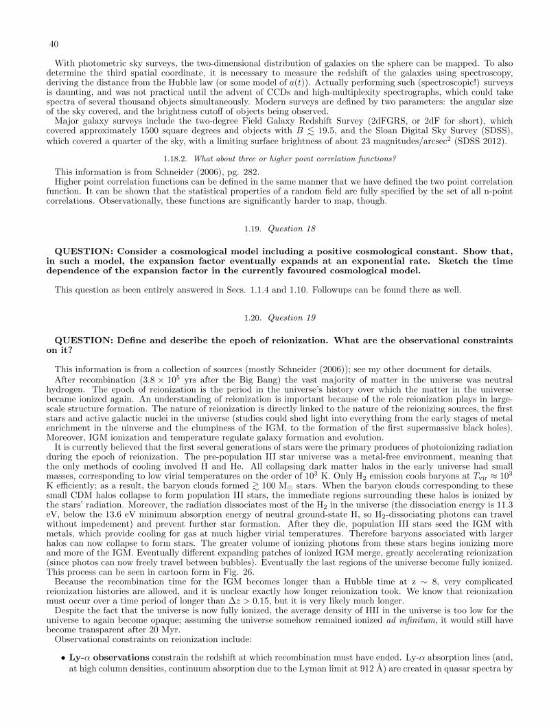
40

With photometric sky surveys, the two-dimensional distribution of galaxies on the sphere can be mapped. To alsodetermine the third spatial coordinate, it is necessary to measure the redshift of the galaxies using spectroscopy,deriving the distance from the Hubble law (or some model of a(t)). Actually performing such (spectroscopic!) surveysis daunting, and was not practical until the advent of CCDs and high-multiplexity spectrographs, which could takespectra of several thousand objects simultaneously. Modern surveys are defined by two parameters: the angular sizeof the sky covered, and the brightness cutoff of objects being observed.

Major galaxy surveys include the two-degree Field Galaxy Redshift Survey (2dFGRS, or 2dF for short), whichcovered approximately 1500 square degrees and objects with B . 19.5, and the Sloan Digital Sky Survey (SDSS),which covered a quarter of the sky, with a limiting surface brightness of about 23 magnitudes/arcsec2 (SDSS 2012).

1.18.2. What about three or higher point correlation functions?

This information is from Schneider (2006), pg. 282.Higher point correlation functions can be defined in the same manner that we have defined the two point correlation

function. It can be shown that the statistical properties of a random field are fully specified by the set of all n-pointcorrelations. Observationally, these functions are significantly harder to map, though.

1.19. Question 18

QUESTION: Consider a cosmological model including a positive cosmological constant. Show that,in such a model, the expansion factor eventually expands at an exponential rate. Sketch the timedependence of the expansion factor in the currently favoured cosmological model.

This question as been entirely answered in Secs. 1.1.4 and 1.10. Followups can be found there as well.

1.20. Question 19

QUESTION: Define and describe the epoch of reionization. What are the observational constraintson it?

This information is from a collection of sources (mostly Schneider (2006)); see my other document for details.After recombination (3.8 × 105 yrs after the Big Bang) the vast majority of matter in the universe was neutral

hydrogen. The epoch of reionization is the period in the universe’s history over which the matter in the universebecame ionized again. An understanding of reionization is important because of the role reionization plays in large-scale structure formation. The nature of reionization is directly linked to the nature of the reionizing sources, the firststars and active galactic nuclei in the universe (studies could shed light into everything from the early stages of metalenrichment in the uinverse and the clumpiness of the IGM, to the formation of the first supermassive black holes).Moreover, IGM ionization and temperature regulate galaxy formation and evolution.

It is currently believed that the first several generations of stars were the primary produces of photoionizing radiationduring the epoch of reionization. The pre-population III star universe was a metal-free environment, meaning thatthe only methods of cooling involved H and He. All collapsing dark matter halos in the early universe had smallmasses, corresponding to low virial temperatures on the order of 103 K. Only H2 emission cools baryons at Tvir ≈ 103

K efficiently; as a result, the baryon clouds formed & 100 M stars. When the baryon clouds corresponding to thesesmall CDM halos collapse to form population III stars, the immediate regions surrounding these halos is ionized bythe stars’ radiation. Moreover, the radiation dissociates most of the H2 in the universe (the dissociation energy is 11.3eV, below the 13.6 eV minimum absorption energy of neutral ground-state H, so H2-dissociating photons can travelwithout impedement) and prevent further star formation. After they die, population III stars seed the IGM withmetals, which provide cooling for gas at much higher virial temperatures. Therefore baryons associated with largerhalos can now collapse to form stars. The greater volume of ionizing photons from these stars begins ionizing moreand more of the IGM. Eventually different expanding patches of ionized IGM merge, greatly accelerating reionization(since photos can now freely travel between bubbles). Eventually the last regions of the universe become fully ionized.This process can be seen in cartoon form in Fig. 26.

Because the recombination time for the IGM becomes longer than a Hubble time at z ∼ 8, very complicatedreionization histories are allowed, and it is unclear exactly how longer reionization took. We know that reionizationmust occur over a time period of longer than ∆z > 0.15, but it is very likely much longer.

Despite the fact that the universe is now fully ionized, the average density of HII in the universe is too low for theuniverse to again become opaque; assuming the universe somehow remained ionized ad infinitum, it would still havebecome transparent after 20 Myr.

Observational constraints on reionization include:

• Ly-α observations constrain the redshift at which recombination must have ended. Ly-α absorption lines (and,at high column densities, continuum absorption due to the Lyman limit at 912 A) are created in quasar spectra by

41

Fig. 26.— A cartoon of the two-step reionization process. At z & 12 population III stars form in low-mass halos, ionizing the nearbyuniverse and dissociating H2 across the universe. When these stars die, they seed the IGM with metals, allowing more metal-rich stars toform in much more massive halos. These metal-rich stars eject many more ionizing photons, and are primarily responsible for reionizingthe entire universe. From Schneider (2006), his Fig. 9.30.

the H i floating in the line-of-sight between us and the quasar (neither free-free absorption nor scattering producesabsorption lines). The n = 1 to n = 2 transition for a neutral H atom translates to a photon of λLyα = 1216 A,meaning that for a QSO at z = zQSO, we could expect any QSO emission between λLyα(1+zQSO)−1 and λLyα topotentially be absorbed by lines. If there were a large amount of H i at all redshifts from 0 to zQSO, the absorptionlines would merger together into a trough - the fact that we do not see this at z <∼ 5 (despite there being enoughhydrogen density) indicates that the universe is currently ionized (the Gunn-Peterson test); otherwise the variouspockets of overdense HI would create a “forest” of absorption lines (Schneider 2006). However, for spectra ofQSR at z & 6, we see signs of strong Gunn-Peterson troughs, indicating that dense patches of H i still existedat z & 6. From this we can set the lower limit for the completion of reionization at z ∼ 6. Unfortunately, Ly-αemission cannot penetrate past regions with neutral fractions greater than about 10−3, meaning that it cannotbe used to probe the era of reionization itself. See Fig. 27.

• The proximity effect is when the QSO ionizes nearby H i clouds, reducing the Ly-α absorption at redshiftsclose to the emission redshift of the QSO spectrum. The size and shape of this damping can tell us the fractionof hydrogen that is neutral in the space around the QSO (giving us an indication of how far reionization hasprogressed).

• CMB polarization measurements can be used to constrain the start of reionization. H ii region electrons havea tendency to Thomson scatter incoming CMB photons. Since this scattering is isotropic, Thomson scatteringblends photons from different regions of the CMB together, washing out anisotropies. Thomson scattering alsohas a natural polarization axis. If in the electron rest frame the CMB were isotropic, no net polarization wouldbe created, but since the CMB itself is anisotropic, CMB radiation can become polarized. The degree of CMBpolarization is directly related to the Thomson scattering optical depth, which is related to when a significantamount of H ii existed in the universe. WMAP three-year observations of CMB polarization suggest the depthis fairly large, indicating that reionization may have started quite early. Because it is measuring an integratedquantity (degree of polarization along the line of sight) WMAP results cannot easily constrain the period of timeover which reionization occured - if it was instant, WMAP gives z = 11.3; if it occurred over an extended periodof time from z ∼ 7 onward, reionization could have begun closer to z = 15.

• 21-cm line emission and absorption from H i could prove an invaluable tool to studying reionization. In

42

Fig. 27.— UV spectra of QSOs near z = 6. Each spectrum contains a prominent and broad Ly-α emission line (intrinsic to the quasaremission spectrum (CHECK) THIS), preceded by a Ly-α forest at lower wavelengths. Near z = 6 the forest is thick, and overall absorptionalong the line of sight is significant. Note in some cases there is slightly less absorption right near the Ly-α emission line - this is due tothe proximity effect, where the QSO ionizes it surrounding IGM (this effect can be used to separate the ionizing flux of photons from theparticular QSR and from the background). The forest flattens near z = 6, indicating the creation of significant Gunn-Peterson troughspast that redshift from passing the emission through thick HI regions. This indicates the universe became fully ionized around z = 6. FromSchneider (2006), his Fig. 9.28.

the late (z . 9) reionization epoch, the 21-cm line intensity is simply proportional to the ionized fraction, andtherefore it is straightforward to translate fluctuations in 21-cm emission to the progression of reionization.While QSO observations are restricted to z . 6 and CMB observations are integrated, 21-cm line emission andabsorption could probe to much higher redshifts while maintaining fidelity in both time and space.

1.20.1. What about He reionization?

This information is from ?.HeII has an ionizing potential energy of 54.4 eV, and the soft emission from population III stars is unable to ionize it

(in contrast, population III stars can easily ionize HeI, with an ionizing potential of 24.6 eV) (Furlanetto & Oh 2008).As a result He only fully ionizes when the quasar population is large enough for large numbers of hard quasar-emittedphotons to percolate the universe, which occurs at z ∼ 3. The most significant observation evidence for reionizationcompletion at z ∼ 3 comes from far-UV studies of the He Ly-α forest along lines of sight to bright quasars, whichshow a significant increase in HeII optical depth near z ∼ 3. Other, more controversial evidence also exists (such asa decrease in the HI recombination rate (which corresponds to a change in HI opacity), a change in the hard photonopacity in the universe, and a change in IGM temperature; observations of these effects are not as conclusive as theLy-α studies). Despite the lack of theoretical studies done on He reionization, it should be noted that the universe atz = 3 is easier to understand and observe than z & 6, and therefore the physics of reionization can be constrained byfurther study of He reionization.

44

2. EXTRAGALACTIC ASTRONOMY (GALAXIES AND GALAXY EVOLUTION, PHENOMENOLOGY)

Due to time constraints all these solutions are based off of Emberson (2012) and last year’s qualifiernotes, including figures, unless specifically cited otherwise.

2.1. Question 1

QUESTION: Sketch out the Hubble sequence. What physical trends are captured by the classificationsystem?

Fig. 28.— The Hubble sequence of galaxy classification. From Emberson (2012).

Hubble produced an empirical morphological classification scheme of galaxies; this is now known as the Hubblesequence (Fig. 28). According to the scheme, these main types of galaxies exists:

• Elliptical Galaxies: These have nearly elliptical isophotes, contours along which their surface brightness isconstant. They are without any clearly defined structure. They are subdivided according to their ellipticityε = 1− b/a, where a and b denote the semimajor and the semiminor axes, respectively. Ellipticals are found overa relatively broad range in ellipticity, 0 ≤ ε . 0.7. The notation En is commonly used to classify the ellipticalswith respect to ε, with n = 10ε (e.g., an E4 galaxy has an axis ratio of b/a = 0.6, and E0’s have circular isophotes.In reality, elliptical galaxies are triaxial in nature, so ε is a function of viewing angle. Misaligned isophotes (i.e.isophotes not concentric with one another) is evidence of triaxiality. Ellipticals vary in size from 10 to 1000 kpc,have MB from -8 to -25, and have masses between 107 and 1014 M. They are deficit in dust and gas, and donot form many new stars.

• S0 (Lenticular) Galaxies: These are a transition between ellipticals and spirals, subdivided into S0 and SB0,depending on whether or not they show a bar. They contain a bulge and a large enveloping region of relativelyunstructured brightness which often appears like a disk without spiral arms. They may also have dust, which isparameterized by subscript numbers running from 1 to 3 (S01 has no dust, S03 has a lot of dust).

• Spiral Galaxies: These consist of a disk with spiral arm structure and a central bulge. They are divided intotwo subclasses: normal spirals (S’s) and barred spirals (SB’s). In each of these subclasses, a sequence is definedthat is ordered according to the brightness ratio of bulge and disk, and that is denoted by a (a bulge-to-diskluminosity ratio of about 0.3), ab, b, bc, c (bulge-to-disk luminosity ratio of 0.05), cd, d. Spirals vary in sizefrom 5 to 100 kpc, have MB from -16 to -23, and have masses between 109 and 1012 M.

• Irregular Galaxies: These are galaxies with only weak (Irr I) or no (Irr II) regular structure. In particular,the sequence of spirals is often extended past Sd to the classes Sdm, Sm, Im, and Ir, and the sequence of barredspirals equivalently so (m stands for Magellanic; the Large Magellanic Cloud is of type SBm). Irregulars vary insize from 0.5 to 50 kpc, have MB from -13 to -18, and have masses between 108 and 1010 M.

Ellipticals and S0 galaxies are often referred to as early-type galaxies, spirals as late-type galaxies. While Hubblehimself believed this to be an evolutionary track (which could make sense if one assumed that spirals are collapsedellipticals), we now known this is not at all the case.

45

Fig. 29.— B − V colour as a function of galaxy morphology. From Roberts & Haynes (1994), their Fig. 5.If we look at the various differences in galaxy properties as a function of morphology, like Roberts & Haynes (1994)

did, we would find the strongest trend to be colour (Fig. 29), and a trend past Sbc galaxies of later-type spiralsgenerally being less massive, less bright, and slightly smaller. The colour trend broadly describes the average age ofstars in the galaxies, which describes their star formation history. Since bulges tend to contain older, redder stars,while disks contain regions of active star formation, the fact that spiral galaxies are bluer than ellipticals is at leastpartly a function of bulge-to-disk luminosity ratio (it is also partly a function of metallicity, since metallicity makesstars redder). Bulges are also held in equilibrium via velocity dispersion σ rather than bulk rotational velocity v, andtherefore later-type galaxies tend to be more v-supported rather than σ-supported. For spirals, later-type galaxies alsotend to have less loosely wound spirals.

2.1.1. What does the Hubble sequence miss?

Fig. 30.— The extended Hubble sequence, plotted as a function of both morphology and luminosity. From Abraham (2011c).

One substantial feature missed in a classification system based only on morphology is luminosity (Fig. 30). As anexample, elliptical galaxies would encompass

• Normal ellipticals: (with a range of MB from -15 to -23, itself divided into giant ellipticals (gEs), intermediateluminosity ellipticals (Es) and compact ellipticals (cEs).

46

• Dwarf ellipticals: much smaller surface brightnesses and lower metallicity than cEs.

• cD galaxies: MB ∼ 25 and R . 1 Mpc galaxies only found near the centres of clusters. They appear to beellipticals (with a de Vacouleurs profile) with an extended exponential envelope.

• Blue compact dwarf galaxies (BCDs): small ellipticals with a relatively blue population and significantamounts of gas.

• Dwarf spheroidals (dSphs): low luminosity and surface brightness (MB & −8).

There are direct correlations between luminosity and other properties of galaxies; see below for the Tully-Fisherrelationship and the fundamental plane.

The Hubble sequence also misses out a large number of galaxy types. The classic sequence neglected irregulars, cDs,BCDs, dSphs, and other very small objects, which make up the vast majority of all galaxies (by number, not by mass).Active galactic nuclei (AGN), starburst galaxies (including luminous infrared galaxies, LIRGs, and ultra-luminousinfrared galaxies, ULIRGs) are also neglected. Galactic evolution is also neglected: merging galaxies make up about3% of all galaxies today, and are not accounted for by the Hubble sequence. At high redshift, however, they make upalmost half of all galaxies (and the rest look more like irregulars than spirals and ellipticals).

2.1.2. What is the Tully-Fisher relationship?

The Tully-Fisher relation is a relationship between a late-type galaxy’s luminosity and the maximum velocity of itsrotation curve (roughly the the value of v in the flat region of the curve):

L ∝ vαmax (51)

where α ≈ 4. This scaling can easily be derived by noting that v2max ∝M/R and L ∝M and assuming L/R2 is roughly

a constant. The Tully-Fisher relationship exists so long as the mass-to-light ratios and the surface brightnesses of late-types is roughly constant (the latter is related to Freeman’s Law, an empirical statement that the central surfacebrightnesses of disks have a very low spread amongst sprials). This is of course not always true, and we can see shiftsin the Tully-Fisher relationship from Sa to Sc due to changing M/L.

2.1.3. What is the fundamental plane?

The Faber-Jackson relation is a relationship between an early-type galaxy’s luminosity and its central velocitydispersion σ0:

L ∝ σ40 . (52)

This can also easily be derived, using the same assumptions as was used to derive the Tully-Fisher relationship exceptfor replacing the centripetal motion equation with the virial theorem, T ∝ σ2 ∝M/R. As it turns out, if we actuallyplotted real early-type galaxies on an L vs. σ4

0 plot, we would obtain a fairly large dispersion, and the situation ismore complicated.

Empirically, Re ∝ 〈I〉−0.83e , where the averaging for I is done over the area of galaxy interior of Re. If we use this

additional piece of information, we can find that L ∝ R2e 〈I〉

−0.83e , which gives us 〈I〉e ∝ L−1.5. Luminosity is also

somehow related to σ0, as we noted earlier with the Faber-Jackson relation. We therefore have a relationship betweenRe, 〈I〉e and σ0, though if we plotted these relationships using real data, we would obtain large dispersions for each.

The true relationship between the three values, derived observationally, is known as the fundamental plane,

Re ∝ σ1.40 〈I〉

−0.85e , (53)

and can be modelled if we assume that the mass-to-light ratio for early-type galaxies increases slightly with mass.

2.1.4. What other criteria could be used for galaxy classification?

Besides morphological criteria, colour indices, spectroscopic parameters (based on emission or absorption lines), thebroadband spectral distribution (galaxies with/without radio and/or X-ray emission), as well as other features mayalso be used for galaxy classification.

2.2. Question 2

QUESTION: What is the total mass (in both dark matter and in stars) of the Milky Way galaxy?How does this compare to M31 and to the LMC? How is this mass determined?

From Binney & Tremaine (2008), pg. 18, the mass of the various components of the MW are: 2+3−1.8× 1012 Mfor the dark matter halo, 4.5± 0.5× 1010 M for the disk, and 4.5± 1.5× 109 M for the bulge, with approximately

47

1/3 of the baryonic mass in gas. The dark matter dominates, by far, and its error is enough to wash out all othercontributions to the galactic mass. The current consensus is that the Andromeda Galaxy (M31) has roughly the same,with M31 probably the slightly more massive of the two. The mass of the LMC is approximately 1 − 2 × 1010 M,which includes its dark matter halo.

For massive nearby galaxies, as well as our own, the total mass is constrained within the first few tens of kpc usingthe Doppler-shifted 21-cm radio emission of the H i disk to determine rotational velocities. If we estimate the entiresystem, including the dark matter, as being axisymmetric out to the furthest extent of H i, then the interior massM(r) can be determined by determining the H i velocity at r

v(r)2 =GM(r)

r(54)

Past the edge of the H i disk, kinematics of particularly bright objects, such as planetary nebulae, globular clustersand satellite galaxies are used instead. Unfortunately, the uncertainties in such techniques are plagued by low samplesizes as well as the fact that there is seldom knowledge of the proper motions of the objects to complement their observedradial velocities and distances (because with low sample size higher order velocity moments cannot be determined).Because of the latter, assumptions must be made on the eccentricities of the satellite orbits thereby affecting the massdetermination. (This is an incarnation of the “mass-anisotropy” degeneracy, where highly elliptical orbits will shiftmass estimates.) As a sketch of how such an estimate is made, let us assume that, over the sampling of objects used,the total enclosed mass does not change significantly. Then, since GM = v2r, the mass can be estimated by

M =C

G

1

N

N∑i

v2r,iri. (55)

vr,i is the radial velocity of object i, C ≈ 32π(3−2〈e2〉) is a corrective term that accounts for the fact that v2

rr/G samples

the projected mass and not the true mass, and⟨e2⟩

can be calculated if the population distribution of eccentricities

is known. This expression converges to the true mass as 1/√N . This method was used to constrain MMW ≈ 3× 1012

M and MM31 ≈ 1× 1012 M using satellite galaxies.To get the mass of the non-dark matter components of a galaxy, we can use photometry and spectroscopy. Pho-

tometry is used to determine the total luminosity of the galaxy, while spectroscopy is used to determine the stellarpopulation, and therefore give a theoretical estimate for the mass-to-light ratio. A stars-to-gas ratio must also bedetermined.

These methods can also be used with smaller galaxies like the LMC, but as an irregular galaxy significantly affectedby the MW’s gravity the LMC does not have a very well-defined rotation curve. Another method of determining themass of satellite galaxies is its tidal radius: since the LMC is gravitationally affected by the MW, past a certain distancefrom the “centre” of the LMC, stars and gas that originally belonged to the LMC would have been cannibalized bythe MW. This distance can be determined by

rt = RLMC

(MLMC

2MMW(RLMC)

)1/3

(56)

where RLMC is the distance to the LMC from the MW, about 50 kpc, and MMW(RLMC) is the mass enclosed withinRLMC. The tidal radius, estimated from the distribution of stars associated with the LMC, is ∼ 10 kpc, and from theabove equation we can determine MLMC ≈ 0.01MMW. Note that we have assumed sphericity of both galaxy potentialwells, which is likely untrue.

2.2.1. Why can’t we simply use the inner 10 kpc data derived from 21-cm line emission and a model of the halo to determinethe mass of the halo?

While an NFW halo6 or isothermal sphere is often assumed as the distribution of dark matter, as we have no realunderstanding of the nature of dark matter it would be foolish to assume that we do not require observations at largedistance to more fully constrain the halo. Moreover, in lenticular and elliptical galaxies, the inner 10 kpc is oftendominated by stellar mass, making it difficult to obtain good estimates of the dark matter halo properties.

2.2.2. How is the total mass of an elliptical galaxy determined?

This answer is mainly from my own work with Anne-Marie.The 21-cm line is often non-existent in early-type galaxies, and satellite galaxy/PNe kinematics have the same low

S/N issues as they do when used on the MW or Andromeda. As hinted at by Eqn. 55, the eccentricity and orbitalorientations of a population of objects can change the enclosed mass estimate substantially. To obtain this information,higher-order terms in the line-of-sight velocity distribution (vr and σr being the first two moments, skew and kurtosisbeing the third and fourth) are required. These cannot easily be obtained through satellite/PNe kinematics (due to

6 Note that the NFW halo profile gives infinite mass if integrated out to infinity. A cutoff (usually the radius at which density drops to200 times the critical density of the universe) is generally imposed to obtain a mass.

48

low S/N), but they can be using stellar kinematics. Early-type galaxies have their matter dominated by stars outto at least 1 Re, and have low surface brightness outside 1 Re. To probe the dark matter halo, therefore, requireseither extensive long-slit spectroscopy or the use of an integral-field spectrograph (and tons of binning). For details,see Weijmans et al. (2009).

2.3. Question 3

QUESTION: How do we know that the intergalactic medium is ionized?

Fig. 31.— A cartoon of how pockets of neutral hydrogen absorb Ly-α from a quasar. From Emberson (2012).

This question is intimiately related to Sec. 1.20 and Sec. 2.14, and indeed are partially answered in those questions.We know the universe’s hydrogen is ionized for two primary reasons:

• Lack of Ly-α absorption: the spectra of high-redshift quasars always display a large number of narrowabsorption lines superimposed on the quasar’s continuous spectrum; these lines are in addition to any broadabsorption lines that are associated with the quasar itself. These narrow lines are formed when the light form aquasar passes through clouds of material in the line of sight between us and the quasar (Fig. 31). The reasonwhy a forest of lines appears is that as the light propagates the entire spectrum, along with any absorption linesformed, redshift. Each absorption line corresponds to the redshifted Ly-α wavelength of an intervening clouds.

Past z = 6, we see the development of a Gunn-Peterson trough, indicating that all light above about 1216 Aisbeing absorbed by intervening clouds. This indicates that a fraction of the IGM is neutral past z = 6. Becausethe Ly-α cross-section is enormous, an extremely low column density (nHI & 10−13 cm−37 is already sufficientto generate a Gunn-Peterson trough. We do not see this for nearby quasars, indicating that almost all hydrogenin the universe is ionized.

• Temperature of the IGM: the temperature of the IGM today is between 105 and 107 K. This requires thatH i be almost completely ionized.

We can also perform an order of magnitude theoretical estimate, a la Jeffrey Fung. There are 1011 galaxies in theobservable universe, with on average 109 stars in them, and let us assume 0.1% of these are O and B stars. Theirluminosity is about 103 L and their emission peaks in the UV, so we can assume all their 2× 1047 photons generatedper second ionize hydrogen. This is a total ionizing photon flux of 2×1063 s−1. There are 1080 H-atoms in the universe,so it takes 1.6 Gyr to completely ionize the universe.

2.3.1. Is He and metals ionized? Is any component of the IGM neutral?

Absorption of quasar emission by He II and partly and totally ionized metals, primarily C and Mg, together with Si,Fe, Al, N, and O. The mix of elements is similar to that found in the interstellar medium of the MW, indicating thatthe material has been processed through stars and enriched in heavy elements. These lines are though to be formedin the extended halos or disks of galaxies found along the line of sight to the quasar.

From a theoretical standpoint, it takes 2.176× 10−18 Z2 J to completely ionize an element with atomic number Z.Setting kBT = 2.176 × 10−18 Z2, and T = 107 K, we obtain Z ≈ 8. This suggests that heavy elements such as Fe orU are not completely ionized.

7 This can be determined using τ = 4× 1010h−1 nHI (z)

(1+z)√

1+Ωmz, where nHI is in units of cm−3. We set τ = 1.

49

2.3.2. What are the properties of these neutral H clouds? Can they form galaxies?

We deduce the size of the intergalactic clouds by comparing the Ly-α forest in the spectra of pairs of lensed quasars.Many of the absorption lines are seen in both spectra, but some are not. This indicates that the clouds are, on average,about the size of the lensing galaxy. From the total calculated column density of hydrogen (ionized plus neutral), themass of atypical cloud is somewhere around 107 M. At the temperate estimated for a typical cloud (T ∼ 3× 104 K,its self-gravity would be too weak to keep it from dispersing. It may be held together by the pressure of less dense(but hotter) external IGM or by the presence of DM within the cloud.

The clouds are placed into three categories. The low column density Ly-α forest absorbers (ΣHI < 1016 cm−2)are associated with the diffuse IGM. These systems probe low-density, highly ionized gas and are thought to tracethe dark matter distribution throughout the IGM as well as contain the bulk of the baryons at high redshift and asignificant amount of the baryons even today. At the other end, the high column density damped Ly-α absorbers(DLAs, ΣHI > 1020 cm−2) appear associated with the main bodies of galaxies. These high-density, predominantlyneutral systems serve as neutral gas reservoirs for high redshift star formation. The intermediate column densitysystems, known as Lyman Limit Systems, mark the transition from the optically thin Ly-α forest to the opticallythick absorbers found in and around the extended regions of galaxies. Typically these absorbers are easy to identifyin QSO spectra due to the characteristic attenuation of QSO flux by the Lyman limit at ∼ 912 A in the rest frame.In addition, they are optically thick enough to be harbouring neutral hydrogen cores.

2.4. Question 4

QUESTION: Describe as many steps of the distance ladder and the involved techniques as you can.What are the rough distances to the Magellanic Clouds, Andromeda, and the Virgo Cluster?

This is mostly from my own notes.The cosmic distance ladder consists of a large number of means to determine (luminosity, for the most part) distances

to objects. They are listed below, and extragalactic ones in Fig. 32. The differing techniques are generally calibratedto one another (to provide consistency), and therefore it is highly advantageous for differing rungs of the ladders tooverlap.

Fig. 32.— Plot of various extragalactic distance-determining techniques, with their maximum effective luminosity distance measureslocated to the left. The various colours represent applicability to different classes of object (but can effectively be ignored). Solid blacklines indicate good calibration between two steps on the ladder; dashed lines indicate poor calibration. “GCLF” is the globular clusterluminosity function, “PNLF” is planetary nebula luminosity function, and “SBF” is surface brightness function. From Wikipedia (2011a).

Solely Galactic distance determining techniques:

• Geometric parallax is the measurement of the position of a distant objects from two different observationpoints separated by some physical distance called a “baseline”. The baseline divided by the angle by which theobjects shifts when moving between the two points of observation gives a distance estimate. The technique isusually only applicable to nearby stars (the Gaia satellite will change this). Commonly the baseline used is the

50

diameter of the Earth’s orbit around the Sun, but the proper motion of the Sun can be used to create longerbaselines.

• The moving cluster method uses the proper motion of cluster members, as well as cluster member radialvelocities, to determine distance to the cluster.

• Dynamical parallax uses measurements of the period (or a related orbital value) and angular semi-major axisof binary stars to determine their distance. By plugging in the period, angular semi-major axis and a mass-luminosity relation into Kepler’s Third Law, one obtains an equation solvable for the distance to the binary.

• Main sequence fitting* of stars in a cluster onto an HR diagram, and comparison of that fit with a similar fitto the Hyades cluster, can be used to determine open cluster distances up to 7 kpc.

• Spectroscopic parallax is the determination of the luminosity of a star from a combination of spectral class andline-broadening (the 2-dimensional Morgan-Keenan luminosity class). Combined with the apparent magnitude,this can be used to determine a distance modulus to the star. Technically spectroscopic parallax is useful up to10 Mpc, but in practice it is only used up to 105 pc.

• Expansion velocities of SNe ejecta proper motion measurements, combined with measurements of radialvelocity from Doppler shifts and the assumption that expansion is spherically symmetric can be combined toobtain distances.

Extragalactic distance determining techniques (some can also be used in our own Galaxy):

• The Wilson-Bappu effect (up to 0.1 Mpc) is a spectroscopic parallax effect where the width of a smallemission line housed in the K absorption line of calcium is correlated to absolute magnitude for G, K and Mstars. Calibrated to geometric parallax, the Wilson-Bappu effect is mostly used for distances up to the LMC.

• Bright red supergiants (up to 7 Mpc) which appear to have the same absolute V and bolometric magnitude.Requires distingishing individual stars, giving it the same range as spectroscopic parallax.

• Tip of the RGB (up to 7 Mpc) is a similar method that uses the tip of the red giant branch star luminosityfunction. Stars travelling up the RGB will eventually experience an He flash and transition off the RGB tothe zero-age horizontal branch. An He flash occurs when the He core of an RGB reaches ∼ 0.5 M, and theluminosity prior is dependent on properties of the H-burning shell, which in turn is dependent on the He core;this means that the most luminous a red giant can get is an almost constant value. A distance, then, can beestimated from the brightest RGB stars in a galaxy (since they will be very near the RGB tip).

• Novae (up to 20 Mpc) have, like their SNe Ia cousins, a luminosity vs. light curve decline time relationship thatallows them to be calibrated into standard candles using Mmax

V = −9.96 − 2.31log10m, where m is the averagerate of decline over the first 2 mag in magnitudes per day. This relationship comes from the fact that moremassive WDs tend to accrete smaller amounts of matter before a nuclear runaway occurs (i.e. producing lessbright an explosion), and this thinner layer is ejected more easily.

• Variables (up to 29 Mpc) have a correlation between pulsation and luminosity8, allowing determination of adistance modulus (assuming extinction is also known). Classical Cephids have been seen up to 29 Mpc away,while RR Lyrae and W Virginis stars are generally fainter and therefore can only be used for closer distances.

• Globular clusters* (up to 50 Mpc) follow an empirical luminosity function. Because the function has aturnover, fitting a sampling of globular clusters around a distant galaxy with the luminosity function can be usedto derive a relative distance.

• Planetary nebulae* (up to 50 Mpc) also appear to follow a luminosity function9 with a rapid cutoff at around-4.6 mag. Fitting, and comparing to a fit with a known distance, provides a distance measure; alternatively,finding the brightest PN in a galaxy and assuming they reside near the cutoff also gives a distance. As the cutoffmethod uses brighter PN, it can be to larger distances (the fitting method only goes up to 20 Mpc).

• The surface brightness method* (up to 50 Mpc) is based on the fact that the number of bright stars (whichcontribute the majority of the brightness) per area element in a galaxy fluctuates by Poisson noise. Since agalaxy further away will subtend a smaller area on the sky, there will be more bright stars per angular area, andtherefore less fluctuation in the surface brightness (since the fluctuation goes like

√N/N).

8 MV = −3.53log10(Pd)− 2.13 + 2.13(B − V ).9 Here the measured luminosity is Lλ at λ = 5007 A.

51

• The Tully-Fisher relation* (> 100 Mpc) is a relation between a spiral galaxy’s luminosity and its maximumrotational velocity described in Sec. 2.1. The analagous relation for ellipticals is the Faber-Jackson relation, andis much noisier and more difficult to use as a standard ruler. Physically, the Tully-Fisher relation means that themass-to-light ratio and mean surface brightness of spirals is fairly constant. In fact, due to the changing fractionof baryons in gas instead of stars for lower mass spirals, the mass-to-light ratio does change - adding a correctionterm to the Tully-Fisher relation results in a much tighter relationship.

• The D − σ relation* (> 100 Mpc) is a relation between an elliptical galaxy’s angular diameter D out to aconstant surface brightness (20.75 B-mag per arcsec) and its velocity dispersion. Since surface brightness isindependent of distance, D is inversely proportional to the distance to the elliptical galaxy. Physically, thisrelation is a natural outcome of the fundamental plane and the (fairly good) assumption that all ellipticals areself-similar.

• Masers (> 1000 Mpc) are amplified microwave emissions coming from regions of interstellar media where popu-lations (due to very low densities) can become inverted. Cosmic masers exist around some galactic nuclear regionswith line luminosities up to 104 L; these maser sources orbit the supermassive black hole, and observations ofboth the radial and proper motions of these sources can be made. If we assume circular orbits, these two valuescan be combined to give a distance. Source radial velocities can also be combined with an independent measureof the black hole mass to determine distances.

• Supernovae Ia (> 1000 Mpc) have (or at least a sub-class of them have) a strong relation between light curvedecay time and peak luminosity, the Phillips relation (Sec. 1.9). While most optical and infrared observations canbe used, this relation is has the smallest spread in the infrared. Other supernovae have similar relationships thatcould be used to determine luminosity (ex. SNe IIP plateau longevity is correlated with maximum luminosity),though these relationships are generally not as well defined and/or studied, and SNe Ia are brighter in the opticaland IR and other SNe.

• Brightest galaxies in clusters* (> 1000 Mpc) fits a luminosity function to the galaxy cluster, and determinesa distance modulus from the fit. It assumes that the luminosity function of galaxies remains fixed over time.

• Cosmological redshift (> 1000 Mpc) requires finding characteristic spectral features (lines, bumps, etc.).Redshift can be made to correspond to a physical distance through Hubble’s Law (v = H0d) at low redshifts,and to dc (assuming a cosmological model) at large redshift. Use of this measure must take into account peculiarvelocities of objects.

All techniques denoted with a * are secondary distance indicators, which only give distance scaling, and thereforerequire a calibration galaxy with a distance known by other means (primary distance indicators can be used on theirown because they give absolute luminosity distances).

The distance to the LMC can be determined from the Wilson-Bappu, RGB tip/supergiants, and variable starmethods, giving a distance of ∼ 48 kpc (the same answer can be obtained by “going backwards” by taking the NGC4258 maser distance as a baseline for other distance measures). The most accurate distance for an object, however,was found using the light echo of SN1987A off of a nearly perfectly circular ring of material (ejected during the SNprogenitor’s AGB phase) to determine a distance. The ring is inclined to us, and so while light from the SN shouldimpact all sections of the ring at the same time, due to the inclination and light delay we see different sections of thering light up at different times. The light delay can be used to determine the physical size of the ring, while its angularsize is easily observed, and from these two measurements we can obtain a distance of 51.8± 3 kpc to the SNR.

The distance to Andromeda has been measured with variable stars, surface brightness fluctuations, RGB tip/supergiants,the Wilson-Bappu effect and measurements of eclipsing binaries; the current accepted distance is ∼ 770 kpc.

The distance to the Virgo Cluster can be determined by using a large number of these methods, including variablestars, novae, luminosity function methods, surface brightness fluctuations, the Tully-Fisher and D − σ relations andType Ia supernovae, applied to its component galaxies; all methods agree that it is ∼ 17 Mpc away.

2.5. Question 5

QUESTION: What evidence is there that most galaxies contain nuclear black holes? How do thoseblack holes interact with their host galaxies?

For most observational purposes, a black hole (BH) is defined as a mass-concentration whose radius is smaller thanthe Schwarzschild radius rS of its corresponding mass. This value is about rS ∼ 107 km ∼ 15 R for the SMBH in theGalactic centre (GC). Since we cannot even resolve the supermassive black hole (SMBH) in our own galactic centre(which spans 10−5”) in order to show that other galaxies contain SMBHs we must find indirect evidence of a massivecompact object at the centres of galaxies.

52

For many galaxies, we can detect stellar kinematics around the galactic centre. The radius of influence of a blackhole is defined as

rBH =GMBH

σ2≈ 0.4 pc

(MBH

106 M

)(σ

100 km/s

)−2

(57)

where the inherent velocity dispersion of the material being affected by the black hole is σ. The equivalent angularscale is

θBH =rBHD≈ 0.1′′

(MBH

106 M

)(σ

100 km/s

)−2(D

1 Mpc

)−1

. (58)

The presence of an SMBH inside rBH is revealed by an increase in σ; σ ∝ r−1/2. If the centre of the galaxy rotates,we would also expect v ∝ r−1/2. The challenge here is to obtain stellar kinematics at resolutions substantially smallerthan θBH ; moreover, the kinematics of stars can be complicated, and the observed values of σ and v depend on thedistribution of orbits and on the geometry of the distribution.

Nevertheless, we have made measurements of the stellar kinematics of nearby normal galaxies, and have found whatappear to be ∼ 107 M highly concentrated masses in approximately 35 of them. In general, the kinematics areincompatible with the r−2 isothermal profile of a star cluster; it is especially well-constrained for our own galaxy. Insome cases, water masers orbiting very close to the galactic centre were used to determine the existence of an accretiondisk around the point masses.

For our own MW galactic centre, we can track individual stars, and we have found stars with proper motionsexceeding 5000 km/s. Combining σ and the trajectories of individual stars, we are able to determine that the enclosedmass M(r) ≈ 4× 106 M down to ∼ 0.01 pc. The closest approach of a star to the object is even smaller, 0.0006 pc.This is not within the Schwarzschild radius (3× 10−7 pc).

We also have active galactic nuclei, and we know that the radio lobes in some of these AGN reach & 1 Mpc, indicatingthat the central power source is long-lived. Luminous QSOs have luminosities of up to L ∼ 1047 erg/s. Combiningthese two numbers gives us E ∼ 1061 erg. Lastly, luminosity variations in some AGN can be up to 50% on the timescaleof days. This means that R . 0.0008 pc. The radio lobes are fairly straight, indicating that the generator must be avery stable rotator. In many AGNs, X-ray observations of a (both special and general) relativistically broadened Feline indicate emission in the inner regions of an accretion disk, with a radius of just a few Schwarzschild radii.

All these observations are not proof of the existence of a SMBH in these galaxies, because the sources from which weobtain the kinematic evidence are still too far away from the Schwarzschild radius. The conclusion of the presence ofSMBHs is rather that of a missing alternative; we have no other plausible model for the mass concentrations detected.We may postulate an ultra-compact dark star cluster with a density profile steeper than r−4, but such a cluster wouldevaporate within 10 Myr due to frequent stellar collisions. The case for AGN being due to SMBHs is stronger. Nosource of energy other than accretion onto a black hole can realistically explain so much energy being generated in avolume of space so small10. Moreover, the Fe line is entirely consistent with an accretion disk that extends down to afew Schwarzschild radii.

Black holes affect their host galaxies in a number of ways, primarily through the outflows they generate when theaccrete:

1. Black holes can quench star formation in the galaxy by generating very strong outflows (i.e. quasar jets) duringrapid accretion (Page et al. 2012; Faucher-Giguere & Quataert 2012). These outflows expel the ISM. It is possiblethat this is why there is a relationship between the mass of the bulge and the mass of the SMBH (Page et al.2012).

2. Closely related to the previous point, black holes limit the growth of massive galaxies. The current luminosityfunction cutoff L∗ corresponds to a halo mass considerably lower than the mass scale above which the abundanceof dark matter halos is exponentially cut off. We also know that massive galaxies were already in place at highredshift, and so should have grown considerably since then via cooling flows. The solution is to invoke AGN- they heat the cooling, infalling material, heating it up and preventing it from forming stars. (Black holestherefore both expel and heat matter, both of which quench star formation.)

3. More dormant black holes can blow x-ray cavities filled with relativistic plasma in the centres of galaxies (Sijackiet al. 2007).

4. Black holes (AGN feedback) may solve cosmic downsizing.

5. Black holes tend to fling hypervelocity stars out of the galaxy through 3-body interaction. A binary systempassing very close to the black hole may result in one star being flung into the black hole, and the other starobtaining an enormous velocity to conserve momentum. A few of these stars (generally early types, as that isthe population of stars near the Galactic centre) have been seen in the MW.

10 Black holes have an accretion efficiency of ∼6 - 29%; a star at the Schwarzschild radius has Egrav ∼ 1053 erg, so to power an AGNrequires some 10−6 M/yr worth of accretion.

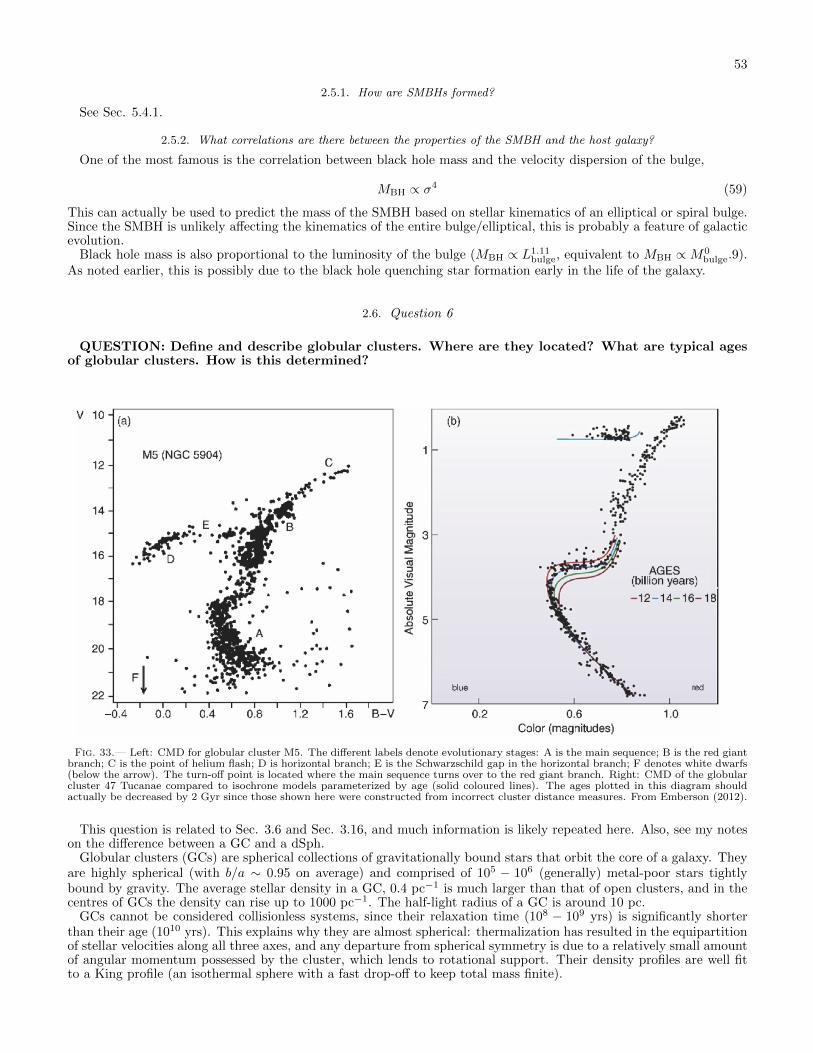
53

2.5.1. How are SMBHs formed?

See Sec. 5.4.1.

2.5.2. What correlations are there between the properties of the SMBH and the host galaxy?

One of the most famous is the correlation between black hole mass and the velocity dispersion of the bulge,

MBH ∝ σ4 (59)

This can actually be used to predict the mass of the SMBH based on stellar kinematics of an elliptical or spiral bulge.Since the SMBH is unlikely affecting the kinematics of the entire bulge/elliptical, this is probably a feature of galacticevolution.

Black hole mass is also proportional to the luminosity of the bulge (MBH ∝ L1.11bulge, equivalent to MBH ∝M0

bulge.9).As noted earlier, this is possibly due to the black hole quenching star formation early in the life of the galaxy.

2.6. Question 6

QUESTION: Define and describe globular clusters. Where are they located? What are typical agesof globular clusters. How is this determined?

Fig. 33.— Left: CMD for globular cluster M5. The different labels denote evolutionary stages: A is the main sequence; B is the red giantbranch; C is the point of helium flash; D is horizontal branch; E is the Schwarzschild gap in the horizontal branch; F denotes white dwarfs(below the arrow). The turn-off point is located where the main sequence turns over to the red giant branch. Right: CMD of the globularcluster 47 Tucanae compared to isochrone models parameterized by age (solid coloured lines). The ages plotted in this diagram shouldactually be decreased by 2 Gyr since those shown here were constructed from incorrect cluster distance measures. From Emberson (2012).

This question is related to Sec. 3.6 and Sec. 3.16, and much information is likely repeated here. Also, see my noteson the difference between a GC and a dSph.

Globular clusters (GCs) are spherical collections of gravitationally bound stars that orbit the core of a galaxy. Theyare highly spherical (with b/a ∼ 0.95 on average) and comprised of 105 − 106 (generally) metal-poor stars tightlybound by gravity. The average stellar density in a GC, 0.4 pc−1 is much larger than that of open clusters, and in thecentres of GCs the density can rise up to 1000 pc−1. The half-light radius of a GC is around 10 pc.

GCs cannot be considered collisionless systems, since their relaxation time (108 − 109 yrs) is significantly shorterthan their age (1010 yrs). This explains why they are almost spherical: thermalization has resulted in the equipartitionof stellar velocities along all three axes, and any departure from spherical symmetry is due to a relatively small amountof angular momentum possessed by the cluster, which lends to rotational support. Their density profiles are well fitto a King profile (an isothermal sphere with a fast drop-off to keep total mass finite).

54

GCs are ubiquitous: they can be found in the halos of almost all galaxies of sufficient mass (including many dwarfgalaxies) are known to have GCs, with the Milky Way having about 150. For our galaxy, they come in two differentpopulations: the metal poor population ([Fe/H] < - 0.8) is spherically distributed, while the more metal rich population([Fe/H] > - 0.8), with the notable exception of 47 Tucana, is primarily distributed near the galactic thick disk, andmay actually be associated with it (both populations having a scale height of 1 kpc and similar rotations about thegalactic centre). GCs can be found from 500 pc to 120 kpc from the galactic centre, though the majority of themare within 40 kpc of the galactic centre. It is not clear whether or not the field stars and some GCs form a unifiedpopulation of halo members.

GC formation history is still not well-understood. They are believed to have formed from the collapse and fragmenta-tion of a single molecular cloud. As a result, the stars within the cluster formed with essentially identical compositionsand within a relatively short period of time. In the MW, tight superclusters like Westurland 1 may be their precursors.

The stellar population of a GC is roughly coeval (though there are exceptions, like NGC 2808, that contain multiplegenerations of stars), i.e. all stars in the cluster have the same age. This allows the stellar population to be fit toan isochrone, a snapshot in time of the evolution of a line of coeval stars. Since isochrones are time-dependent, theage of the best-fitting isochrone gives an estimate of the mass of the GC (there are various methods of doing this; see(Binney & Merrifield 1998, Ch. 6.1.4)). Fig. 33 gives two examples.

The mean age of the oldest globular clusters around the MW is 11.5±1.3 Gyr, though absolute ages are often greatlyaffected by errors on GC distances and reddening (De Angeli et al. 2005). The dispersion in ages of metal-poor MWGCs is about 0.6 Gyr De Angeli et al. (2005). Higher-metallicity clusters are on average 1 - 1.5 Gyr younger, thougha rare few are younger stil De Angeli et al. (2005).

An interesting feature evident in the colour-magnitude diagrams of young globular clusters is the Hertzsprung Gap.This is the paucity of stars located between the turn-off point of the MS and the RGB. This feature arises because ofthe rapid evolution that occurs just after leaving the MS. The evolution of this stage is largely damped for low massstars (1.24 M) and so this gap does not appear for old globular clusters where the turn-off point is located at lowmass scales. Another interesting feature seen in some globular clusters is the existence of a group of stars, known asblue stragglers, that can be found above the turn-off point (i.e., still on the MS). Although our understanding of thesestars is incomplete, it appears that their tardiness in leaving the MS is due to some unusual aspects of their evolution.The most likely scenarios appear to be mass exchange with a binary star companion, or collisions between two stars,extending the star’s MS lifetime.

2.7. Question 7

QUESTION: What is the X-ray background and how is it produced?

This information is mostly from my own notes.

Fig. 34.— Left: comparison of SED measurements of the CXB. Here E2dF/dE, which is dimensionally equivalent to λFλ. Right: SEDof cosmic background radiation, plotted as νIν versus λ. Besides the CMB, background radiation exists in the radio domain (cosmic radiobackground, CRB), in the infrared (CIB), in the optical/UV (CUVOB), in the X-ray (CXB), and at gamma-ray energies (CGB). With theexception of the CMB, probably all of these backgrounds can be understood as a superposition of the emission from discrete sources. Theenergy density in the CMB exceeds that of other radiation components. From Emberson (2012).

In the 1960s and 1970s, rocket and satellite-based x-ray observatories began discovering strong galactic and extra-galactic x-ray sources. In addition to these sources, however, they also detected an isotropic x-ray background that(at first) did not seem to be caused by any known source - this background has come to be known as the cosmicx-ray background (CXRB, or CXB). It was hypothesized early on that the background was due to a large number of

55

unresolved point-source AGNs, but AGN spectra have power laws Sν ∝ ν−0.7 (Sν is the source function) while theCXB can roughly be parameterized by Iν ∝ E0.3 exp(−E/E0), where E0 ≈ 40 keV.

Later, deep (i.e. able to distinguish faint sources) ROSAT observations showed that at least 80% of CXB emission inthe 0.5 - 2 keV band can be attributed to discrete sources (predominantly AGN, but also starburst and normal galaxies,and galaxy clusters at large distance); later XMM-Newton observations would confirm this. Because of their spectralindex AGN could not account for the CXB at high energy even if they contributed 100% of 0.5 - 2 keV CXB emission.Instead, the high energy CXB could be dominated either by enshrouded AGN (whose intrinsic spectrum would bemodified by interactions with the shrouding material) or by pockets of superheated gas in the IGM with energieskT ≈ 30keV (a popular hypothesis, since the CXB spectrum, subtracted by the AGN contribution from ROSAT,gave a very hard (i.e. flat) spectrum reminiscent of thermal bremmstrahlung). This same gas, however, would inverseCompton scatter CMB photons, producing distortions to the CMB blackbody. Hot IGM gas was therefore eliminatedas a high-energy CXB contributor when COBE observations showed negligible blackbody distortion.

More recent observations from Chandra in the 2 - 10 keV range have shown at least 75% of the CXB at this energyrange can be resolved as descrete x-ray sources, most of which are AGN with strong self-absorption. AGN with strongself-absorption are Type 2 AGN, which have only been detected with Chandra (indicating why the high-energy CXBmystery was not resolved until its launch).

It is currently believed that a large population of AGN are believed to have column densities larger than NH ≈1.5 × 1024 cm−2, corresponding to τ = NHσT ≈ 1 (where σT is the Thomson scattering cross-section). Known as“Compton-thick” AGN, they are extremely difficult to detect, as much of the x-ray spectrum is downscattered byCompton scattering. At very high energies, these systems can still be detected, and form part of the CXB. Sincetelescope resolution is poor, the CXB then currently forms the primary means by which we can constrain the spacedensity of Compton-thick AGN. Ultimately, however, discrete sources must be found, and their summed emissioncompared to the CXB; recent and near future hard x-ray surveys, as well as attempts to find high-redshift AGN inthe IR (highly shrouded AGN will have their black hole UV emission reprocessed into the IR) will likely provide thediscrete source densities needed to explain the high-energy CXB.

2.7.1. What determines the emission spectrum of an AGN?

See Sec. 2.13.

2.7.2. Are there backgrounds at other wavelengths?

Fig. 34 shows a large number of different cosmic backgrounds. As discrete sources were not removed from the figure,discrete sources such as galaxies and quasars are included in all the backgrounds.

The cosmic infrared background (CIB) was first discovered in the far-IR by COBE. It, like the CXB, is most likelydue to a large unresolved population of discrete sources (such as high-redshift starburst galaxies). Unfortunately theCIB is very difficult to detect due to instrument cooling limitations and the fact that the CIB is much fainter than thegalactic infrared background. As of 2006 most of the sub-mm CIB has been determined to be due to dusty star-formingregions and other discrete sources, while the ISO satellite has managed to resolve about 10% of ∼ 2 µm emission asdiscrete sources.

Indeed, the other cosmic backgrounds are likely entirely due to discrete sources, as well, since we do not expect high-energy backgrounds to have cosmological origin. The CRB is likely due to a combination of the CMB and radio-loudgalaxies, the CUVOB entirely due to stars, and the CGB from compact objects, AGN and cosmic ray-ISM interactions.

See Sec. 2.14.

2.8. Question 8

QUESTION: Describe the currently accepted model for the formation of the various types of galaxies.What are the lines of evidence to support this model?

As noted from Sec. 1.4, in concordance cosmology halos of lower mass form first, and massive halos form later. Sincethese massive halos will have smaller halos embedded in them, the formation of a massive halo can be thought of asdue to the merging of smaller halos - this is known as hierarchical structure formation, or the “bottom-up” scenarioof structure formation. If stars formed in these smaller halos, the mergers would be visible.

The formation of spiral galaxies can easily be explained by this picture. Suppose that gas in a halo can coolsufficiently for stars to form (see the cold flows follow-up for discussion). Cooling is a two-body process (∝ ρ2), sothe most efficient coolers will be dense clumps. These dense clumps will have some non-zero angular momentum, andwill therefore settle onto a disk, and thus a small disk galaxy is formed. This process may look like a small-scaleversion of the “monolithic collapse” hypothesis of how the MW formed (Sec. 3.16). Spiral arms are formed by densityperturbations in the disk, which generates waves of star formation in the galaxy. The galaxy can then grow by mergingwith other galaxies. We note, however, that there is no reason to simply expect mergers to continue building the disk(one can imaging various scenarios in which the total angular momentum of the system is much smaller than the spinangular momentum of each galaxy), and disks can be warped and destroyed by merger. Semi-analytical models ofgalaxy formation suggest that the bulge of a spiral is first formed through a major merger, and then the disk is formedthrough gas-rich minor mergers and accretion of cold flows from the IGM.

56

Several proposals have been made on how ellipticals can form. It is possible that ellipticals form by truncatedmonolithic collapse. In the MW monolithic collapse scenario, early star formation lead to the creation of the galactichalo and globular clusters. If all stars were to form this quickly, then an elliptical would be formed before any of thegas could settle onto a disk. It is not obvious how this could occur, however.

Currently ellipticals are generally thought to be formed out of major mergers of disk galaxies. The merger woulddestroy the disks of both initial galaxies, and shock the gas, generating a starburst. Due to the violence of suchmergers, stars and gas are ejected from the system, and remaining gas becomes strongly heated, quenching furtherstar formation after the starburst. Because the stars within ellipticals are generally old, it is suspected that mostmergers that form ellipticals are gas-poor (“dry”), in order to minimize the effect of the starburst.

Evidence for this model:

• We see a plethora of small, irregularly shaped blue galaxies at high redshift, as well as substantial numbers ofgalaxy mergers11.

• Ellipticals tend to show signs of complex evolution that might be produced by mergers.

• The model provides a partial explanation for the Butcher-Oemler effect (clusters contain more blue galaxies athigh redshift)12.

• The model also provides an explanation for the morphology-density relation, where ellipticals are much moreabundant in the centres of dense clusters, while spirals dominate in less dense clusters and in the periphery ofdense clusters.

• Detailed simulations of merging disk galaxies have shown they can produce ellipticals. Simulations indicate thatdry mergers can preserve the fundamental plane (i.e. if, pre-merger, the merging galaxies obey the fundamentalplane, then so will the merger remnant).

• High-luminosity ellipticals tend to have boxy isophotes and are slowly rotating. Low-luminosity ellipticals tendto be more rapidly rotating and have disky isophotes. This can be explaind by dry-mergers generating massiveellipticals and more gas-rich mergers between late-type galaxies generating lower-luminosity ellipticals (early-typegalaxies tend to be more massive than late-type galaxies).

2.8.1. What are cold flows?

This information is from the introduction and conclusion of Brooks et al. (2009).The classic model for galaxy formation, loosely describe above, has the dark matter violently relaxing and virializing

very quickly during the non-linear collapse phase. This process shock-heats the infalling baryons to virial temperaturesas well. Given some kind of density profile, a cooling radius can be calculated, and in the interior gas radiates awaythermal energy while maintaining its angular momentum. Recent numerical studies have shown evidence to thecontrary: that much of the infalling baryonic matter is never shock-heated to virial temperatures, and flows onto acold disk without out the need for substantial dissipation. Brooks et al.’s simulations find that early disk growthcan largely be attributed these cold flows, even if most of the inflowing gas is shock-heated to virial temperatures.This gas does heat up somewhat from loss of its own gravitational potential energy, but still substantially below virialtemperatures. For an MW mass galaxy, only ∼25% of the accreted gas comes from acquiring other galaxy halos, andso most of the stars are formed out of cold flow material. This picture allows large disks to be built at much higher zthan the classical model.

2.8.2. What is feedback?

Shortly after the formation of stars, the most massive of them explode as supernovae, which reheat the ISM aroundthem. This reduces the cooling rate of the gas (and also blows some gas away). AGN and stellar winds from OBassociations provide similar “feedback” mechanisms that help regulate star formation. Without this, the amount ofstar formation predicted by numerical simulations would far outpace the rate observed in nature. Indeed, massivegalaxies would likely be much more massive, and luminous, without feedback, a fact suggested by the L∗ turnofftranslating to a much smaller halo mass than the M∗ turnoff predicted by evolution of the matter power spectrum.

The combined efforts of AGN and starburst feedback mechanisms are also responsible for maintaining the highionization level in the IGM, which serves to maintain a high kinetic and excitation temperature in the IGM. Largehalos are more affected by their own internal radiation output than intergalactic ionizing radiation. For smaller halos,however, this effect is important, and suppresses star formation as well as lowers the baryon fraction (by makingbaryons escape the potential well). Since these small halos are also disproportionately affected by their own feedbackmechanisms (SNe are not less powerful because they are in less massive galaxies!). This is a potential solution forthe “missing satellites problem”, where there are far fewer small galaxies in the universe than there should be given aPress-Schechter DM halo distribution.

11 This is buoyed theoretically: D+(z) evolution suggests that cosmic evolution slows substantially after z = 1, meaning the rate ofmergers slows.

12 The other part of the explanation is that ram-pressure stripping removes gas from galaxies over time.

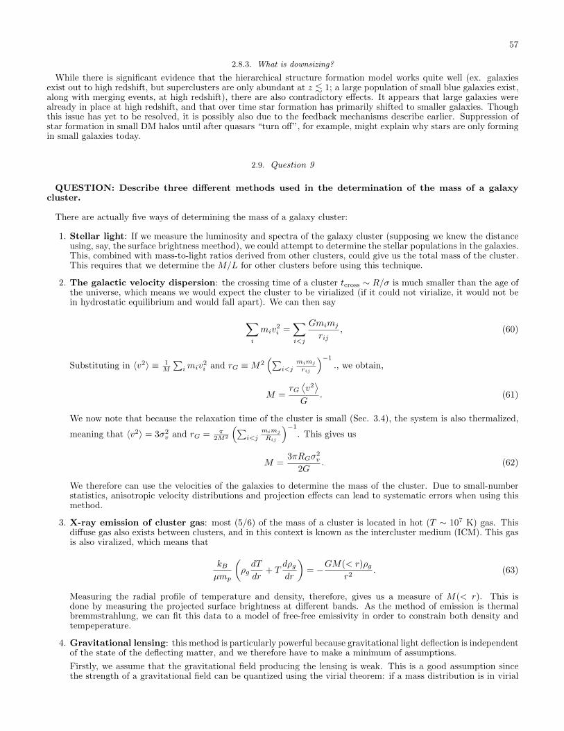
57

2.8.3. What is downsizing?

While there is significant evidence that the hierarchical structure formation model works quite well (ex. galaxiesexist out to high redshift, but superclusters are only abundant at z . 1; a large population of small blue galaxies exist,along with merging events, at high redshift), there are also contradictory effects. It appears that large galaxies werealready in place at high redshift, and that over time star formation has primarily shifted to smaller galaxies. Thoughthis issue has yet to be resolved, it is possibly also due to the feedback mechanisms describe earlier. Suppression ofstar formation in small DM halos until after quasars “turn off”, for example, might explain why stars are only formingin small galaxies today.

2.9. Question 9

QUESTION: Describe three different methods used in the determination of the mass of a galaxycluster.

There are actually five ways of determining the mass of a galaxy cluster:

1. Stellar light: If we measure the luminosity and spectra of the galaxy cluster (supposing we knew the distanceusing, say, the surface brightness meethod), we could attempt to determine the stellar populations in the galaxies.This, combined with mass-to-light ratios derived from other clusters, could give us the total mass of the cluster.This requires that we determine the M/L for other clusters before using this technique.

2. The galactic velocity dispersion: the crossing time of a cluster tcross ∼ R/σ is much smaller than the age ofthe universe, which means we would expect the cluster to be virialized (if it could not virialize, it would not bein hydrostatic equilibrium and would fall apart). We can then say

∑i

miv2i =

∑i<j

Gmimj

rij, (60)

Substituting in 〈v2〉 ≡ 1M

∑imiv

2i and rG ≡M2

(∑i<j

mimjrij

)−1

., we obtain,

M =rG⟨v2⟩

G. (61)

We now note that because the relaxation time of the cluster is small (Sec. 3.4), the system is also thermalized,

meaning that 〈v2〉 = 3σ2v and rG = π

2M2

(∑i<j

mimjRij

)−1

. This gives us

M =3πRGσ

2v

2G. (62)

We therefore can use the velocities of the galaxies to determine the mass of the cluster. Due to small-numberstatistics, anisotropic velocity distributions and projection effects can lead to systematic errors when using thismethod.

3. X-ray emission of cluster gas: most (5/6) of the mass of a cluster is located in hot (T ∼ 107 K) gas. Thisdiffuse gas also exists between clusters, and in this context is known as the intercluster medium (ICM). This gasis also viralized, which means that

kBµmp

(ρgdT

dr+ T

dρgdr

)= −GM(< r)ρg

r2. (63)

Measuring the radial profile of temperature and density, therefore, gives us a measure of M(< r). This isdone by measuring the projected surface brightness at different bands. As the method of emission is thermalbremmstrahlung, we can fit this data to a model of free-free emissivity in order to constrain both density andtempeperature.

4. Gravitational lensing: this method is particularly powerful because gravitational light deflection is independentof the state of the deflecting matter, and we therefore have to make a minimum of assumptions.

Firstly, we assume that the gravitational field producing the lensing is weak. This is a good assumption sincethe strength of a gravitational field can be quantized using the virial theorem: if a mass distribution is in virial

58

equilibrium then v2 ∼ Φ where Φ is the gravitational potential. Weak fields are then characterized by v2/c2 1and with v ∼ 1000 km/s for galaxies in clusters this is well justified. Next, we assume that the deflecting masshas a small extent along the line-of-sight, as compared to the distances between the observer and the lens and thelens and the source. A system satisfying this configuration is known as a geometrically thin lens. Since clustersare typically 8 Mpc across, this assumption is justified for sufficiently distant clusters.

If we approximate both the background object and lens as points, we can use Eqn. 214 to determine masses.Since neither the lens nor the mass distribution will be symmetric, the analysis needed is more complicated. Ingeneral, lensing models are constructed and fitted to observed arcs. The more images spread over a greater area,the better the precise distribution of masses in the lens can be determined.

5. The Sunyaev-Zel’dovich effect: described in Sec. 2.18.

Exactly what galaxy clusters are is described in Sec. 2.16.

2.9.1. What are cooling flows?

The outer regions of clusters have very long cooling times, so our assumption of hydrostatic equilibrium for deter-mining the temperature and density of hot gas, above, is valid. Near the centres of galaxies, however, the free-falltime and cooling timescale are of the same order of magnitude. Since cooling (equivalently the free-free emissivity)is a function of ρ2, the collapsing process is a runaway. These “cooling-flows” have been observed at the centres ofmassive clusters, in the form of a sharp peak of X-ray emission.

2.10. Question 10

QUESTION: What is the density-morphology relation for galaxies? How is that related to what weknow about the relationship between galaxy density and star formation rates in galaxies?

The density-morphology relation is the observation that in denser environments, such as galaxy clusters, there is ahigher ratio of elliptical galaxies versus spiral compared with field galaxies. This is true between different clusters, aswell as within a cluster: the central regions of a cluster have a high fraction of elliptical galaxies, while the outskirtshave a relatively lower fraction. See Figs. 35 and 36. The density-morphology relation is also seen in galaxy groups,though for these groups, the increase in the fraction of S0 galaxies as a function of redshift is much more dramaticthan in clusters.

This relationship between morphology and density can (see Sec. 2.1) be translated into a colour-density relation.Galaxies exist in two groups: the blue clump and the red sequence. Since earlier-type galaxies are redder, we expectthe red sequence to dominate over the blue clump at the centres of clusters, and the blue clump to dominate the redsequence in low-density regions. This is indeed the case.

Fig. 36 suggests a physical cause for the effect. For R & Rvir, the fraction of the different galaxy types remainsbasically constant. In the intermediate regime, 0.3 . R/Rvir . 1, the fraction of S0 galaxies strongly increasesinwards, whereas the fraction of late-type spirals decreases accordingly. Below R . 0.3Rvir , the fraction of S0 galaxiesdecreases strongly, and the fraction of ellipticals increases substantially. This can be explained in the following way: inthe intermediate regions of clusters, a variety of interactions between galaxies and their environment, including ram-pressure stripping, encounters with other galaxies and gas evaporation, turn spiral galaxies into S0 galaxies. Deeperinside the cluster, the merger rate becomes very large due to the high galaxy density, which efficiently generatesellipticals out of other galaxies.

This relation suggests that star formation in a galaxy is a function of the galaxy’s environment: namely, starformation of galaxies in dense environments is either halted or accelerated, in order for the gas within these galaxiesto be quickly be depleted. As a result, the stellar populations in these galaxies look much redder than those of theirpeers in the outskirts of the cluster. We can identify a number of effects:

• Ram pressure stripping: caused by the fast motion of a galaxy through the ICM, which causes a pressurefront to build up at the leading edge of the galaxy. This pressure front heats gas within the galaxy, and, if it isstrong enough, also ejects gas from the galaxy.

• Galaxy strangulation: occurs as a galaxy falls into the cluster for the first time. The gravitational potentialof the cluster creates tidal effects that launch gas out of the galaxy.

• Galaxy interactions: these tend to disturb or radically alter the morphologies of galaxies. Interactions cantidally induce starbursts, generate warps and bars in disks, and eject mass. A long series of slow interactionsare believed to the main driver for turning spirals into S0 galaxies through the thickening of their disks and thetriggering of starbursts in their bulges. Fast interactions are nicknamed “galaxy harrassment”.

• Galaxy mergers: these are more extreme versions of interactions. They tend to both eject gas (through heatingit and pulling it into tidal tails) and trigger starbursts. Indeed, in dense environments, repeated mergers tend

59

Fig. 35.— Fraction of E, S0 and S galaxies as a function of projected galaxy density (units of galaxies/Mpc2). From Emberson (2012).

Fig. 36.— Left: same as Fig. 35, except from SDSS data. Note the point at which the lines begin to curve over is around 1 galaxy/Mpc2.“Intermediates” are mainly S0 galaxies, and “early disk” Sa galaxies. Right, morphology fractions for clusters, as a function of radius fromthe centre of the cluster. From Emberson (2012).

to transfer most of the kinetic energy of the bulk motion of galaxies into kinetic energy of stars and gas. Thisis the reason why the velocity dispersion of very luminous (and therefore more massive and denser) clusters islower than that of less luminous clusters.

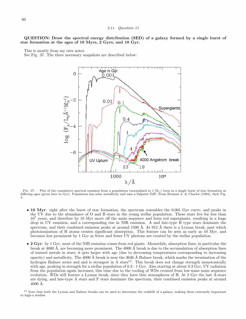
60

2.11. Question 11

QUESTION: Draw the spectral energy distribution (SED) of a galaxy formed by a single burst ofstar formation at the ages of 10 Myrs, 2 Gyrs, and 10 Gyr.

This is mostly from my own notes.See Fig. 37. The three necessary snapshots are described below:

Fig. 37.— Plot of the cumulative spectral emission from a population (normalized to 1 M) born in a single burst of star formation atdiffering ages (given here in Gyr). Population has solar metallicity and uses a Salpeter IMF. From Bruzual A. & Charlot (1993), their Fig.4.

• 10 Myr: right after the burst of star formation, the spectrum resembles the 0.001 Gyr curve, and peaks inthe UV due to the abundance of O and B stars in the young stellar population. These stars live for less than107 years, and therefore by 10 Myr move off the main sequence and form red supergiants, resulting in a hugedrop in UV emission, and a corresponding rise in NIR emission. A and late-type B type stars dominate thespectrum, and their combined emission peaks at around 1500 A. At 912 A there is a Lyman break, past whichphotoionization of H atoms creates significant absorption. This feature can be seen as early as 10 Myr, andbecomes less prominent by 1 Gyr as fewer and fewer UV photons are created by the stellar population.

• 2 Gyr: by 1 Gyr, most of the NIR emission comes from red giants. Meanwhile, absorption lines, in particular thebreak at 4000 A, are becoming more prominent. The 4000 A break is due to the accumulation of absorption linesof ionized metals in stars; it gets larger with age (due to decreasing temperatures corresponding to increasingopacity) and metallicity. The 4000 A break is near the 3646 A Balmer break, which marks the termination of thehydrogen Balmer series and and is strongest in A stars13. This break does not change strength monotonicallywith age, peaking in strength for a stellar population of 0.3 - 1 Gyr. Also starting at about 0.3 Gyr, UV radiationfrom the population again increases, this time due to the cooling of WDs created from low-mass main sequenceevolution. WDs still feature a Lyman break, since they have thin atmospheres of H. At 2 Gyr the last A-starsare dying, and late-type A stars and F stars dominate the spectrum; their combined emission peaks at around4000 A.

13 Note that both the Lyman and Balmer breaks can be used to determine the redshift of a galaxy, making them extremely importantto high-z studies.

61

• 10 Gyr: not much has changed since 2 Gyr. Late-type G stars and K stars dominate the spectrum, which nowpeaks at around 6000 A.

These snapshots are created using population synthesis, which requries knowledge of the stellar initial mass functionand stellar evolution. Of the two, the form has much more uncertainty.

2.11.1. Describe population synthesis.

Let SλZ(τ)(t) be the spectral emission, normalized to 1 M, of a stellar population (determined using an initial massfunction; see Sec. 3.1) with zero-age metallicity Z(τ) and age t. We note that τ = tage− t, where tage is the time sincethe first stars were born in the entire population 14. Multiplying this with the star formation rate ψ(τ) (ψ is definedsuch that star formation starts at τ = 0) gives us ψ(tage − t)SλZ(tage−t)(t) the spectra emission from all stars in thepopulation of age t. The spectral luminosity of a stellar population with age tage can then be found using:

Fλ(tage) =

∫ tage

0

ψ(tage − t)Sλ,Z(tage−t)(t)dt. (64)

Practically, such an integral is done numerically. Moreover, finding both ψ and S are difficult to achieve, and un-der/overestimating the formation of even a single class of stars can significantly change Fλ.

H ii emission, the primary contributor of line emission to galaxies, is generally also added to spectra. After about107 yrs the emission from gas nebulae becomes negligible.

There are very few places in the universe where one can view an isolated stellar population created from a singleburst of star formation - certainly, galaxies look more complex. A more realistic star formation history is

ψ(t) = τ−1 exp(−(t− tf )/τ)H(t− tf ), (65)

where H is the Heaviside function and tf is the time of star formation. τ , the characteristic duration of star formation,as a large effect on the spectrum, because continuous star formation replenishes the supply of hot blue stars that tendto dominate the spectrum. For the same reason, an impromptu burst of star formation can significantly change theoverall shape of the spectrum.

It is practically far more difficult to obtain spectra of galaxies than photometric observations, especially in deep-field surveys. Quite often, then, theoretically calculated spectra are reduced to colours by multiplying them with thetransmission curves of colour filters.

Currently population synthesis can explain the colours of present-day galaxies, but not uniquely - a number ofpossible star formation histories all fit empirical data. Moreover, there is an age-metallicity degeneracy: contours ofconstant colour in an age/metallicity plot have the form

d ln(T )

d ln(Z)≈ −3

2, (66)

i.e. smaller values of Z result in bluer looking spectra and a smaller mass-to-light ratio. Intrinsic dust absorptionwill also redden galaxies.

2.11.2. What do the spectra of real galaxies look like?

From our analysis above we would expect that younger stellar populations have blue spectra, strong emission lines,small 4000 A breaks and weaker absorption lines. Indeed, this is what we see in Fig. 38. Different galaxy types forma continuum from irregulars, which are dominated by blue continuum emission and emission lines, to E0s, which haveprominent absorption lines below 5000 A (in particular the 4000 A break is prominent), no emission lines, and has redcontinuum emission.

2.12. Question 12

QUESTION: What are Lyman-Break Galaxies and how do we find them?

High-redshift galaxies are very faint, and therefore difficult to resolve spectroscopically. As a result, it was nearlyimpossible until recently to actually conduct surveys for high-redshift galaxies. A major breakthrough in findinghigh-z objects is the Lyman-break method, which allowed the discovery of substantially redshifted galaxies throughbroad-band photometry15.

14 This can easily be seen: the first stars in the entire population to be born had metallicity Z(τ = 0), but are currently age t; stars thatare just being born have age t = 0, but have metallicity Z(τ = tage).

15 Narrowband photometry had also been used, specifically to look for the Ly-α emission line. This proved difficult because no one knewhow faint galaxies are at z = 3, and how relatively the Ly-α line would be (Schneider 2006, pg. 357).

62

Fig. 38.— Spectra of galaxies of different types, ranging from very late (Irr) to very early (E0). Flux is plotted in arbitrary normalizedunits, and if my understanding is correct each spectrum has been artificially normalized to fit on the plot. From Schneider (2006), hisFig. 3.50.

Fig. 39.— Principle of the Lyman-break method. The histogram shows the synthetic spectrum of a galaxy at z = 3.15, while the solidspectrum belongs to a QSO at slightly higher redshift. The dotted lines represent three different broad-band filteres. Both galaxies wouldbe seen prominently in G and R, but not in Un; equvialently G−R would be be negative, while Un−G would be positive. From Schneider(2006), his Fig. 9.2.

Since H i is abundant and its ionization cross section is large, we expect photons with λ < 912 A have a low probabilityof escaping from a galaxy without being absorbed. Intergalactic absorption also contributes (as evidenced by the Ly-αforest), absorbing photons with rest-frame wavelengths beyond Ly-α. From this, we expect that galaxies, especiallyhigh-redshift galaxies where the IGM may be partly neutral, are far less bright at wavelengths below 912(1 + z) A,where z is the redshift of the galaxy.

We therefore can formulate an observing strategy to detect high-redshift galaxies (Fig. 39). We choose several

63

broad-band filters λi (three at minimum) with differing central wavelengths. If we find a source which can be seenin all filter images i + 1 and beyond, but is not visible in all filter images before and including i, then we wouldsuspect that we have found a galaxy at redshift z, such that λi . 912 A(1 + z) . λi+1. The z we find is known as a“photometric redshift”. We can equivalently compare colours between filters, and would find that the colour would bevery red between filters i and i + 1. To make sure this is truly a break, we can also test to see if the colour betweenfilters i + 1 and i + 2 is relatively blue. The galaxy candidate detected is known as a Lyman-break galaxy (LBG) ordrop-out.

This method has been used to detect galaxies out to z ∼ 10.

2.12.1. What have we learned about high-z galaxies from LBGs?

Since we require the colour between filters i+ 1 and i+ 2 to be blue, we tend to select for high-z galaxies undergoingactive star formation.

Surveys for LBGs can be used to determine their spatial distribution, and therefore their clustering, as a functionof redshift. Comparing this distribution to the distribution of dark matter halos at the same redshift. We find LBGstend to correspond to high-mass dark matter halos, and tend to be assembled in proto-clusters. LGBs tend to havestrong, blueshifted absorption lines, which could be evidence of feedback outflows from the many SNe generated byhigh star formation rates.

2.12.2. Are there other “breaks” that could be used to detect galaxies?

The Lyman-break technique is a special case of a general method of estimating the redshift of an object usingdrop-out in a photometric band. Though less strong than the Ly-α break, the 4000 A break can also be used forphotometric redshift measurements (this break is particularly strong in early-type galaxies). In general, a series ofstandard spectra can be convolved with the response of different colour filters, thus producing a template that can beused with photometric surveys. In general, photometric redshifts are estimates - to get an accurate redshift detailedspectroscopic follow-up must be performed.

2.12.3. Can we find Lyman-break galaxies at low redshifts?

The Lyman-break at low redshifts lies in the UV. The recent influx of GALEX data has been quite useful in the searchfor low-redshift analogs to LBGs. The result was the discovery of two populations: one composed mostly of normallate-type spirals, and the other composed mainly of compact galaxies with few stars, but the same star formation rateas much larger galaxies. Correspondingly, their stellar populations are more metal-poor. These compact galaxies arelikely related to LBGs.

2.13. Question 13

QUESTION: Draw a spectrum of a high-redshift quasar. What do quasar emission lines typicallylook like? Explain what we see in the spectrum at rest wavelengths bluer than 1216 A.

Quasars belong to a class of objects known as AGN, which is described in more detail in Sec. 2.15. Due to the angleat which we view their cores, the majority of observed luminosity comes from the compact, parsec-sized core of thegalaxy.

The spectrum of a quasar can be found in Figs. 40 and 41. A number of notable features exist:

• The continuum spectrum of a quasar at long wavelengths can be parameterized by

Sν ∝ ν−α. (67)

α ≈ 0.7 for quasars in the radio regime, indicating optically thin synchrotron emission, though if one looks atthe compact core α is much closer to zero due to synchrotron self-absorption.

• There is a substantial increase in emission over this power law (Fig. 41) in the IR, optical and UV. These aredue to thermal emission of the various heated components of the AGN (warm dust in the IR, the accretion diskin the UV).

• The optical and UV spectra of quasars are dominated by numerous strong and very broad emission lines. Thewavelengths are what we would typically expect in an H ii region. The broadening is due to Doppler shifting ofthe gas rapidly orbiting around the black hole at several hundred rs with speeds v ∼ 104 km/s. The gas residingat these distances from the SMBH constitute a broad-line region (BLR) for line emission. Quasars also shownarrow line emission, with Doppler widths suggesting v ∼ 500 km/s. This is due to gas in the narrow-line region(NLR) for line emission, which extends to up to 100 pc from the centre of the AGN. These narrow lines are notdue bulk velocities of the gas, but rather heating: AGN jets heat this region up to 1.6× 104 K.

64

Fig. 40.— Combined spectrum of a sample of 718 individual quasars transformed into rest wavelengths of the sources. The most prominentemission lines are marked. From Emberson (2012).

Fig. 41.— Spectrum of QSO PKS0405-123 (“sum”) broken up into multiple labelled pieces. The accretion disk continuum emission isfurther broken down into the outer, middle and inner disk contributions. The higher frequency bump on the accretion disk is the “big bluebump”. The Balmer continuum is the continuum created by a forest of H line emission from n = 2 to various higher states. Line emissionis from the BLR and NLR. The “power law” is due to accretion jet synchrotron radition. From Schneider (2006), his Fig. 5.20.

• By the x-rays, the intrinsic spectrum of the AGN drops back down to a power law with α ≈ 0.7. Most of theemission in the soft x-rays comes from the inner accretion disk, while most of the harder x-rays come from anon-thermal source (hence the power law).

• Emission short of the rest-frame 1216 A of the AGN may be absorbed, both by pockets of H i in the AGN itself, aswell as the IGM on its way to us. This produces the Ly-α forest, and the lines in the forest can either be narrow,of intermediate width (due to Lyman Limit Systems) or broad (Damped Lyman Limit Systems). If a substantial

65

amount of neutral H i exists in between the quasar and us, we will obtain severe damping at wavelengths above1216 A(1 + z) (where z is the redshift of the quasar); this is known as a Gunn-Peterson trough.

2.13.1. What is the cause of the various emission features of AGN?

AGN intrinsic emission is shaped by the AGN’s various different regions. Thermal emission from the accretiondisk provides the broad IR to UV continuum that peaks in the “big blue bump” in the UV (this bump is usually notdirectly observed; its empirical existence is extrapolated from UV and soft x-ray observations). For blazars, the opticalcontinuum is dominated by power-law continuum emission, likely due to synchrotron radiation from the accretion jets.Warm dust contributes a second bump in the mid-IR.

The broad IR to UV excess is caused by emission from different parts of the accretion disk. Suppose a parcel of massdm at a radial distance r from the black hole drops by distance dr. Taylor expansion of the gravitational potentialenergy gives us dE = GMdmdr/r2. If half (from the virial theorem) of this liberated energy is expelled as heat(radiation), this gives dL = GMmdr/2r2. We can assume the disk is a blackbody, radiating from the top and bottomsurfaces of the disk, in which case dL = 2× 2πrdrσSBT

4. Equating the two dLs together gives us (see Sec. 5.13)

T (r) =

(3GMm

8πσSBr3

)1/4

. (68)

We can rewrite this (see Schneider pg. 187) as

T (r) =

(3c6

64πσSBG2

)1/4

m1/4M−1/2

(r

rS

)−3/4

. (69)

From this we can easily see that for a large enough range of r we obtain a large range of T . Emission from the accretiondisk can then be described, at least to first order, by a superposition of blackbodies (see Fig. 41).

Overlaid on top of this broad thermal emission is a power law, ostensibly from synchrotron radiation. Because ofbeaming effects, the strength of this power law is highly dependent on viewing angle. The spectral index will alsochange with viewing angle - α ∼ 0 is seen with blazars, while α ∼ −1 quasars, and so on.

AGN spectra also contain broad and narrow emission lines. No broad forbidden transition lines are observed,indicating that atoms emitting broad emission lines only have time to perform allowed and semi-forbidden transitionsbefore suffering a collision with another atom - from this we obtain a density on the order of n ∼ 109 cm−3 forthe gas clouds doing the emitting. From line strength ratios, we know the clouds are at T ∼ 2 × 104 K, and, fromline-broadening, they are travelling at around 104 km/s. Comparing the emission measure (photons per unit volumeof the emitting gas) with the line strengths we note that these clouds are fairly small. The space covered by thiscollection of clouds constitutes the “broad line region” (BLR). Reverberation mapping studies 16 of this region showthat these clouds occupy a significant range of radii from the supermassive black hole, and consequently differentdistance clouds have different emission properties (in accordance with their temperature). Not very much is knownabout the kinematics of these clouds, or why their high temperatures do not result in them disintegrating (that couldeither be due to them constantly being replaced, or due to magnetic, pressure or gravitational stabilization.

The narrow (emission) line region (NLR) rotates at a significantly slower rate (∼ 400 km/s) than the BLR, andthe abundance of forbidden transitions indicates a much lower density (∼ 103 cm−3); line strength ratios give T∼ 1.6× 104 K. The region extends out to 100 pc (and is not homogeneous throughout), and because of this large sizecan be resolved - the NLR is cone-shaped, rather than spherically symmetric.

X-ray emission comes from the innermost part of the accretion disk, indicated by the extremely short time periods forvariability. Spectrally, the emission can be characterized as Sν ∝ ν−0.7 to first order; to second order, this functionalform does not account for the big blue bump at low energies, and the spectrum flattening out at high. In additionthere are a number of x-ray emission and absorption lines. For details on these lines, see Sec. 2.15

Some AGN have large H column densities that enshroud the AGN along our line of sight (these are known as Seyfert2 and type-2 QSOs; they are likely the same objects as their type 1 counterparts, seen from different viewing angles).X-rays can photoionize H, and because photoionization absorption decreases with increasing frequency (i.e. energy),lower energy emission is attenuated while higher energy emission is not as affected. These objects are consequentlyvery difficult to detect in the soft x-rays, and type-2 QSOs have only recently been found by (higher resolution hardx-ray observations from) Chandra and XMM-Newton.

2.14. Question 14

QUESTION: Sketch the SED from the radio to gamma of extragalactic radiation on large angularscales. Describe the source and emission mechanism for each feature.

16 Reverberation mapping uses the coupling between the AGN SMBH and the dense clouds to determine the extent of the BLR. Due tolight lag the coupling will naturally have a delay, which can be measured by careful timing of variations in the AGN continuum emissionversus the strengths of different lines. Different lines will show different couplings, since hotter clouds will tend to have more high-energyemission lines.

66

Kissin (2012) gives good information on this topic.

Fig. 42.— The background radiation SED of the universe: (1) radio, (2) CMB, (3) FIRAS excess, (4) DIRBE background (points witherror bars), (5) optical background, (6) UVB, (7) the ISM photoionization optical depth (right-hand scale) for 1019, 1018, and 1017 Hatoms cm−2, (8) soft X-ray background, and (9) high-energy background. From Emberson (2012).

The cosmic background is due to a combination of a uniform background and a large number of point sources. Itcan be seen in Fig. 42, but a better, labelled picture can be found in Fig. 34, right. The cosmic background hasnumerous peaks and troughs, each of which pointing to a different emission mechanism and source.

The cosmic background is split up into:

• The cosmic radio background (CRB): follows a power law in its spectral flux density, with α ≈ 0.6. Thissuggests synchrotron radiation. Since normal galaxies are not strong radio emitters, and diffuse IGM wouldsubstantially inverse Compton scatter the CMB (not seen), it is likely this emission is due to quasars, radiosupernovae and star-forming regions in galaxies. Current estimates (from counting discrete sources) suggestquasars and radio supernovae are minor contributors. To account for the rest of the CRB, star-forming regionswould produce a much larger far-IR background than observed. This suggests another, hitherto unknown,component of the CRB, or a fundamental shift in the nature of the sources at higher redshift.

• The cosmic microwave background (CMB): this is due to photons escaping during last scattering at z ≈ 1100.It has been redshifted from its original λ ≈ 1 µm to today’s 1.1 mm. The CMB is a near-perfect blackbodycentred at 2.73 K.

• The cosmic infrared background (CIB): traditionally difficult to observe because of strong IR absorptionin the atmosphere and emission from the MW, the CIB is likely thermal emission from heated dust in regulargalaxies at low redshifts, LIRGs (1011 L . LIR . 1012 L) at z ∼ 1−2 and ULIRGs (LIR & 1012 L) at z & 2.Obscured AGN provide a minor component as well.

• The cosmic optical background (COB): traditionally difficult to see because of airglow and zodiacal light.Most of it is likely thermal emission from ordinary stars in galaxies with z < 10. AGN accretion, supernovaeand particle decay make up minor components.

• The cosmic ultraviolet background (CUVB): difficult to see for the same reasons as for the COB, as well asreflection of UV light from stars off of the ISM. Extragalactic UV is actually quite low. The main contributor islikely UV light scattered off the ISM in other galaxies, and hot IGM (thermal bremmstrahlung), though somespeculate that redshifted Ly-α emission from recombination might contribute somewhat.

• The cosmic x-ray background (CXRB): discussed in Sec. 2.7.

• The cosmic γ-ray background (CGB): produced by a combination of blazars (beamed synchrotron) andcosmic ray/ISM interactions in star forming galaxies (pion production). Dark matter annihilation may also bea source.

67

2.14.1. Are there non-EM backgrounds?

The cosmic neutrino background is predicted from neutrino decoupling at z ∼ 1010. Because they were never heatedby electron-positron annihilation at the end of lepton pair production, their current temperature, ∼ 1.9 K, is evenlower than that of the CMB. Because neutrinos at these energies have tiny cross-sections, they are nearly undetectable.

The cosmic gravitational wave background is predicted from a combination of discrete sources (inspiralling binaries,mergers, supernovae) and primordial GWs.

2.15. Question 15

QUESTION: What are AGNs? Describe different observational classes of them and how they mayrelate to each other.

This is mostly from my own notes.An active galactic nucleus is a small region at the centre of a galaxy that shows highly luminous non-thermal emission

that is strong over a broad range of the EM spectrum (often clear from radio to gamma). This is significant becauseif one were simply superimpose the spectra of the stellar population in these galaxies, the resulting spectrum wouldgenerally only stretch from 4000 A to 20,000 A (modulo recent star formation, which would add more UV, and dustextinction, which would bump up the far-IR). Moreover the luminosity of these central regions are often on the sameorder of magnitude as all other sources of radiation in the galaxy, making the source of this luminosity unlikely to bedense stellar populations.

The various classes of AGN are unified by the idea that all AGN emission is ultimately caused by accretion ofmaterial by supermassive black holes (SMBHs). Observational differences between AGNs can be explained due toorientation and line-of-sight extinction between their respective SMBHs and observers.

Galaxies are said to have AGN based on the following properties:

• Variability across the spectrum, with amplitude and frequency of variation increasing with respect to time.

• Extended radio emission, often in the form of jets.

• Continuum emission broadly described by a single power law (Sν ∝ ν−α). Emission is often highly polarized (inthe core not as much, but in the extended regions up to 30%)- this fact, combined with the spectral indicies,suggests relativisitc synchrotron emission. This component decreases with weaker AGN.

• Extremely broad emission lines: the broad-line emission regions of AGN cores often have line FWHMs of ∼10000 km/s, while the “narrow’-line region line FWHMs are still around ∼ 100 km/s. These components becomedifficult to observe with weaker AGN.

• Low local space density: Seyferts make up ∼ 5% of spirals, while quasars are extremely rare locally.

AGN contain the following subclasses:

• Seyfert galaxies are ordinary spiral galaxies that also appear to have very luminous nuclear regions with muchbroader emission lines than expected from normal spirals.

– Seyfert 1 galaxies contain both broad and narrow lines. Their overall spectra resemble those of QSOs,and Seyfert 1 and weaker QSOs form a continuum (with the only difference between the two classes beingtheir total luminosity; QSOs are 21 magnitudes brighter than Seyfert 1s).

– Seyfert 2 galaxies contain only narrow lines. Seyfert 1 and 2 galaxy sub-classes form a continuum; Seyfert1.5 or 1.8 galaxies are sometimes referred to.

• Radio galaxies are ordinary ellipticals that have particuarly strong radio emission. They spectroscopicallyresemble radio-loud Seyferts.

– Broad-line radio galaxies (BLRGs) contain both broad and narrow lines. A continuum exists betweenBLRGs and quasars.

– Narrow-line radio galaxies (NLRGs) contain only narrow lines. A continuum exists between NLRGSand BLRGs.

• Quasars are point-like in the optical (originally misidentified as galactic stars), with a very blue spectrum andbroad emission lines. They tend to have high redshift, meaning they are extremely bright, especially for theirsize.

– Radio-loud quasars (or quasi-stellar radio sources; QSRs) have strong radio emission.

68

– Quasi-stellar objects (QSOs) are identical to quasars in the optical, but have very little radio emission.Found (on purpose) by photometric surveys looking for quasars in the optical. A continuum exists betweenquasars and QSOs, leading to the two terms sometimes being used interchangeably.

• Blazars are very similar to OSOs, except they appear to have very rapid (often over days) and greatly varyingoptical emission. This emission is also significantly more polarized (several % polarized) compared to that ofQSOs (. 1%).

– Optically violent variables (OVVs) are QSOs that show substantial variation in the optical over veryshort periods of time.

– BL Lacertae objects (BL Lacs) resember OVVs (fast, extreme variation in the optical, polarized emission)but have spectra completely devoid of emission lines. During their epochs of low luminosity, some BL Lacswill actually appear to morph into OVVs, suggesting a continuum between OVVs and BL Lacs.

• LINERs (low ionization nuclear emission regions) are not traditionally considered AGN (they, for example, areleft out of Schneider), but are still characterized by line strengths that are hard to reproduce with a superpositionof stellar spectra, combined with a slight UV excess. LINERs appear to be lower-luminosity versions of AGN,and there perhaps is a continuum between LINERS and Seyferts or radio galaxies. They are fairly common inthe universe: over half the all local spirals show LINER activity.

See Fig. 43.

Fig. 43.— A comparison of optical (∼ 300 - 600 nm) spectra of various classes of AGN. From Keel (2002).

Since AGN are all dominated by their SMBHs, it is to be expected that all AGN can be described by some combinationof accretion rate ratio m/mEdd and mass of the black hole M . M can explain the transition from Seyfert Is to QSOS,and BLRGs to quasars.

Discussion above also suggest a high degree of anisotropy in emissions, which suggests that absorption and scatteringcan explain the transition between certain AGN types. This is further reinforced by polarization measurements, whichshow narrow-line AGN will often also have fainter, highly polarized broad line emission hidden within their SEDs(which can be isolated using a polarizer). This suggests that the difference between a narrow-line radio galaxy orSeyfert and their broad-line counterparts is the obscuration of the broad-line emitting regions by dust and gas. Wewould also expect “type 2” quasars and QSOs. Chandra and XMM Newton recently discovered QSOs enshrouded

69

in regions with high hydrogen column density (as a result soft x-rays suffer high amounts of extinction); these QSOscontribute to the cosmic x-ray background issue described earlier. ULIRGS (ultra-luminous infrared galaxies) mayalso be type-2 QSO candidates, as they have similar luminosities but emit almost entirely in the IR.

Relativistic beaming affects AGN jets. If we suppose rest frame emission is isotropic (and for a cloud of electronsit should be) and the jet moving along some direction at velocity v, an observer viewing the jet at an angle φ withrespect to the jet direction of motion will see the emission boosted by:(

1

γ(1− β(1− cosφ)

)2+α

, (70)

where β = v/c and α is the rest frame emission spectral index. This boosting greatly increases the flux we recievefrom an incoming jet, and equivalently decreases the flux we recieve from a jet moving away from us. This explainswhy, in general, only one jet can easily be detected 17. This beaming is what makes blazars so bright, and fact thatblazars can be divided into OVVs and BL Lacs is due to the strong dependence on angle near φ = 0. Synchrotron(as noted earlier) is also polarized, which explains why blazars have polarized emission. Relativistic beaming alsoamplifies changes in luminosity, so any minute change in the AGN (which can occur quickly) equals a large change inthe resulting emission.

AGN jets plow through their host galaxies, eventually dispersing into enormous radio lobes. It is believed that thesynchrotron from the extended lobes is due to electrons being accelerated to relativistic speeds by shock-heating ofthe ISM and IGM by the jets.

How to connect radio loud and radio quiet systems is not entirely resolved, since there is more than one way to unifyAGN. Schneider suggests that it may be due to galactic morphology (radio galaxies are ellipticals, while Seyferts arespirals). While there is a link between galactic and AGN luminosity, it is not obvious what morphology has to do withanything. Another proposal (also seen in Schneider, and Fig. 44 is suggestive of this as well) is that radio-loud/quiethas something to do with spin of the black hole - since accretion jets are created by the winding of magnetic fields,this is an understandable relation.

Fig. 44.— Scheme for unifying AGN. The progression from narrow-line galaxies to strong line to quasar/QSO to blazar depends onviewing angle. The difference between Seyferts and radio galaxies is explained as a matter of a lack of synchrotron emitting accretion jets(perhaps due to the spin of the SMBH?). From Abraham (2011a).

17 The same is true at the kpc scale; the (still relativistic) jet coming toward us is far brighter than the jet going away. This is corroboratedby the fact that in cases where two jets are seen, the faint jet appears to have undergone additional Faraday rotation compared to thebright jet, indicating it went through more of the galactic ISM to reach us.

70

2.15.1. Where are most AGN located?

Quasars and QSOs in particular have a space density vs. redshift distribution that peaks at z ∼ 3.3, and tails off oneither side. The reason for this is likely galactic evolution of some kind (ex. at higher redshifts there are fewer largeblack holes, at closer redshifts these black holes are not fed as well).

2.15.2. What evidence is there that AGN are powered by supermassive black holes?

This is covered in other questions as well, but we will treat it in detail here.The size and structure of the jets/lobes of AGN requires an enormous power source that “points” in a constant

direction for a time on the order of 107 yr. Bright AGN have luminosities up to 1047 erg/s; if this were constant for107 yr 1061 erg is required, an enormous source of energy. AGN luminosity may change significantly on the timescaleof hours; since information propagates at the speed of light global variations in emitted power must be the result ofchanges in a very compact source (R ≈ 1015 cm if we use ∆t = R/c, where ∆t is the variation timescale.

It is essentially impossible for this nuclear source to come from, for example, a dense star cluster. Fusion, at best,can derive 0.008mPc

2 worth of energy per nucleon - this translates to > 109 M required if one assumes an AGNlifetime of > 107 yr. The Schwarzschild radius of a 109 M system is RS ≈ 1015 cm, the same order of magnitudeas the compact source radius derived above (and much larger than the RS of a 106 M SMBH). Strong gravitationaleffects cannot, then, be avoided even if a black hole is not assumed.

The only other reasonable power source is gravitational potential energy via accretion. Accretion onto a black hole,for example, has an efficiency ε (i.e. in εmc2) of anywhere between 6% (for non-rotating BHs) and 30% (BH withmaximum allowed angular momentum). Luminosity from steady-state accretion is Eddington luminosity limited; if weassume L = LEdd, we obtain, by inverting Eqn. ??, a mass estimate of 106 M for Seyferts and 108 for QSOs. Such alarge mass in a region so small would require that the mass be contained in a supermassive black hole (SMBH); thisconclusion is also consistent with the fact that using gravitational potential energy would still require the dumping of109 M into a tiny region of space.

An SMBH power source is also consistent with a number of other observations. Firstly, the “big blue bump”mentioned in a previous question can be explained as blackbody radiation from the superheated accretion disk. Thebulk motion of radio jets is also highly relativistic (from direct observations and the requirement for shock-heatedelectrons to produce synchrotron radiation in the lobes), and in many astrophysical processes the velocity of ejectedmaterial is on the same order of magntude as the escape velocity of the system. Also, relativistic jets suggest escapefrom a black hole. Rotating SMBHs naturally act like gyroscopes, allowing them to create straight jets. X-ray emissionline profiles can also be explained by emission conditions near the SMBH event horizon; see Fig. 45.

Fig. 45.— Line emission from near the event horizon of the SMBH, and how the emission is modified by both special relativity (theemitter is moving relativistically) and general relativity (the emitter is near the SMBH event horizon). From Schneider (2006), his Fig.5.16.

2.16. Question 16

QUESTION: What are galaxy clusters? What are their basic properties (eg, mass, size). List andexplain three ways they can be detected.

71

Galaxies are not uniformly distributed in space, but instead show a tendency to gather together into gravitationallybound collections known as galaxy groups and galaxy clusters. The transition between groups and clusters of galaxiesis smooth. The distinction is made by the number of their member galaxies. Roughly speaking, an accumulation ofgalaxies is called a group if it consists of N . 50 members within a sphere of diameter D . 2 Mpc. Clusters haveN & 50 members and diameters between 2 and 10 Mpc. Typical values for the mass of a cluster are M ∼ 1014 M formassive clusters, whereas for groups M ∼ 1013 M is characteristic, with the total mass range of groups and clustersextending over 1012 M .M . 1015 M. Alongside the cluster there is a substantial amount of intercluster medium(diffuse gas), and due to the massive gravitational potential a cluster this gas is hot, and the galaxies have high pecularvelocities (∼ 1000 km/s). In fact, on average galaxies make up only a few percent of the total mass of a cluster, whileICM makes up about 10% and dark matter about 90% (Wikipedia 2012e).

Methods of detecting galaxies include:

• Looking for clustering in the optical: pioneered by Abell in the 1950s. Clustering is detected by requiringa large number (in Abell’s case, ≥ 50) of galaxies in a magnitude range (m3 ≤ m ≤ m3 + 2, where m3 is theapparent magnitude of the third brightest galaxy in the cluster) within a certain angular radius (θ = 1.7′/z).Abell determined redshift by assuming that the 10th most luminous galaxy in any given cluster has the sameluminosity as one in any other. While Abell was limited by the sensitivity of photographic plates, modernsurveys such as SDSS can probe up to significant redshifts using this method. Redshifts are then determinedphotometrically for each galaxy to disentangle projection effects and determine true 3D clustering.

• X-ray emission: hot gas inside clusters have characteristic thermal bremsstrahlung luminosities of 1043 erg/sin the x-ray alone, spread over a size of several Mpc. X-ray surveys looking for such emission are not mired byprojection effects like optical surveys are (i.e. redshifts are unecessary).

• The Sunyaev-Zel’dovich effect (SZ effect): inverse-Compton scattering of the CMB by hot electron gas. Thiseffect is not redshift-dependent, and therefore is extremely useful (if it can be measured, which is difficult) fordetermining the locations of high-redshift clusterse. See Sec. 2.18.

• Weak gravitational lensing: weak lensing is often used to map the matter distribution of known clusters, orto look for cosmic shear (Sec. 1.15), but it can also be used to find clusters. The advantage to using lensing isthat it traces the true mass of the cluster; if a cluster contained very few stars and gas, it could still be detectedby lensing. Lensing is subject to projection effects: it may not always be reasonable to assume only one lensalong the line of sight.

• Red cluster sequence (RCS): early-type galaxies belonging to a cluster have very similar colours, only weaklydepending on their luminosity (this is a metallicity effect - more massive galaxies are more metal-rich). Thesecolours become bluer at higher redshifts - this correlation is so good that redshift can actually be determinedusing it. This relationship exists because the stars contained in the centres of clusters finished forming soon afterthe birth of the universe, and star formation has been minimal since. Strips of galaxies in CMDs of galacticsurveys therefore indicate clusters. See Fig. 46.

Fig. 46.— Colour-magnitude diagram of the cluster of galaxies Abell 2390, observed with the HST. Star symbols represent early-typegalaxies, identified by their morphology, while diamonds denote other galaxies in the field. The red cluster sequence is clearly visible. FromEmberson (2012).

72

2.16.1. How are high-z cluster found?

RCS and the SZ effect are largely redshift-invariant, and therefore work well to find clusters at high z. It can also beassumed that AGN track clustering, and deep imaging using narrow-band photometry centred around 1216 A(1 + z)(to pick out rest-frame Ly-α emission from galaxies) have found high-z clusters.

2.17. Question 17

QUESTION: Describe and give results from simulations of large scale structure in the universe. Whatrole do they have in understanding the formation of large scale structure and Galaxy formation? Whatare their limitations?

Simulations have, in recent years, been instrumental in understanding large-scale structure formation in the universe.This is because, as a whole, gravitational dynamics is far too complicated to be explored fully with analytical or semi-analytical methods. In recent years, computers have achieved enough processing power for hydrodynamics to also beaccounted for, and modern smoothed-particle hydrodynamics (SPH) simulations are routinely used to simulate theevolution of large-scale structure in the universe.

In a typical SPH code, we insert a series of particles, representing dark matter, gas and stars, into a box of comovinglength L with periodic boundaries (often, dark matter alone is used, but modern simulations will also add in gasand stars). Each particle represents a certain mass, and so density is easily obtained by determining the number ofneighbours within a certain volume around one particle. The choice of L limits the scale of the largest features thesimulation can resolve (and so generally L > 200h−1 Mpc). The periodic boundaries means that that we assume oneside of the box connects to the opposite side (and particles that pass through one side of the box reappear on the otherside) - in this way, we can estimate the forces due to objects outside the box. Forces are generally calculated usingNewtonian physics, with the addition of a softening length (i.e. F = GM2/(r + a)2, where a is the softening length)to prevent artifical close-encounters between particles (since in reality we do not expect our matter to be composed ofmassive point sources). Calculating forces on a particle p is a process that takes an amount of time ∝ N2, where Nis the number of particles. As a result, methods such as the Barnes-Hut tree or the particle-particle-mesh are used.Both methods bin masses at large distances from p18. Pressure forces can be calculated by using the particles as anirregular mesh to determine bulk properties of the fluid; the number of particles used in this mesh define a “smoothinglength” - detailed variations in fluid properties cannot be captured at smaller resolutions. The initial conditions tothe simulation can be determined by placing particles in accordance with a Gaussian random field with the powerspectrum P (k, z).

We can clearly see some limitations to the physical model described above:

• We have to make approximations to calculate gravity with reasonable speed. We also have to define a smoothinglength to prevent gravity calculations from diverging. We have to interpolate over multiple particles to deter-mine hydrodynamic forces. All these effects collectively set resolution limits on our simulation, and we cannotdetermine details more fine than this limit. If these details affect evolution on larger scales, we will not capturethe evolution, either.

• A related problem is that we have defined set masses for our particles, which are much larger than the trueindividual masses of dark matter particles. This sets a mass limit - we cannot describe associates of less massiveobjects.

• We cannot discern phenomena that occur only on scales larger than L; if these affect smaller scales, we will notcapture them.

• We generally use Newtonian dynamics. This is often fine, since typical speeds in simulations are << c, andtypical densities are below those where GR would significantly change things.

• Perhaps most importantly, it is extremely difficult to simulate magnetohydrodynamics, turbulence, feedback,radiation transport, and other physics (that generally act on small scales) in these simulations. The effectsof them can be characterized by ad hoc insertions and simplifications, but this may generate biases in thesimulations.

These simulations have shown that matter tends to form Mpc-spanning high density filaments that link togetherto form a web of material across the universe. Between them are large voids with densities much lower than thecosmological average.

18 The tree code determines the nearest neighbours to a particle, which generates a network of neighbours from which closer and moredistant objects to p can be determined; the particle-particle-mesh method determines the distribution of masses by binning masses into a3D grid, and then taking a fast Fourier transform. This gives a smoothed mass distribution that can replace interparticle force calculationsat large distances.

73

Fig. 47.— Simulation by the VIRGO Consortium using 2563 particles in box of side length 240 Mpc/h for different cosmological models:Ωm = 0.3, ΩΛ = 0.7 (ΛCDM), Ωm = 1.0; ΩΛ = 0.0 (SCDM and τCDM); Ωm = 0.3, ΩΛ = 0.0 (OCDM). The two Einstein-de Sitter modelsdiffer in the shape of their power spectra. Simulation parameters were chosen so that large scale structure at z = 0 is statistically identicalbetween them - their differences lie at high redshift. From Emberson (2012).

On large scales simulations have allowed us to test ΛCDM cosmology against other universes. Fig. 48 shows thatvarying cosmological parameters will result in statistical differences between the matter power spectrum (and thereforecorrelation between galaxies) of the universe. This can be tested against observations of high-redshift galaxy clustering,and results have borne out in favour of ΛCDM.

Large scale simulations can also be used to test the Press-Schechter model for dark matter halo growth (by binninghalos found in simulations by mass); simulations to date have shown Press-Schechter to, as a whole, be quite accurate,with numerically derived fitting formulae being only slightly different. This is astonishing, since Press-Schechter doesnot take into account non-linear evolution, while simulations do. Press-Schechter tended to underestimate the numberof high-mass halos, and overestimate the number of low-mass ones. These very high mass halos collapse early inthe simulations, and often continue to grow until they become the centres of massive galaxy clusters. If these halosrepresent quasars, they would support the claim that rare objects such as quasars can be formed in a ΛCDM universe.

Simulations can also be used to determine the two-point correlation function of galaxies, and how well this functiontraces the dark matter correlation function. As it turns out, there is a deviation at small scales.

On smaller scales, simulations have shown that dark matter halos have a universal density profile. Averaged overspherical shells, they resemble the Navarro-Frenk-White (NFW) profile:

ρ(r) =ρs

(r/rs)(1 + r/rs)2. (71)

The two free parameters ρs and rs work together to determine both the total mass (inside r200, the radius at whichρ(r) = 200ρcrit) and how concentrated the halo is. Other simulations have slightly different profiles, possibly due totheir treatment of small scales. There is yet no analytical explanation for this profile; moreover, observations of stellarkinematics disagree with the NFW profile near the centres of galaxies (this is known as the “cusp-core war”). Another

74

issue with small scale numerical simulations is that for a given halo, a large number of sub-halos appear embedded init. So far, despite efforts with microlensing, halo substructure within a galaxy has not been observationally confirmed.Moreover, one interpretation of these sub-halos is that they are satellite galaxies. If this were the case, the number ofsatellite galaxies around the MW and other local galaxies is far lower than expected from simulations (the “missingsatellite problem”).

2.18. Question 18

QUESTION: What is the Sunyaev-Zel’dovich effect and where is it detected? What are some chal-lenges in using SZ measurements to determine the values of the cosmological parameters?

The Sunyaev-Zel’dovich (SZ) effect occurs when high-energy electrons (often from the ICM, which, as we have notedin other questions has temperatures around 107 K; high-energy electrons can also be found in the diffuse IGM, andnear the MW) inverse Compton scatter low-energy CMB photons to higher energies. Since this scattering is isotropic,the number of photons headed toward us from the CMB remains fixed; it is the energy of each photon that differs.See Fig. 48.

Fig. 48.— The influence of the SunyaevZeldovich effect on the cosmic background radiation. The dashed curve represents the Planckdistribution of the unperturbed CMB spectrum, the solid curve shows the spectrum after the radiation has passed through a cloud of hotelectrons. The magnitude of this effect, for clarity, has been very much exaggerated in this sketch. From Emberson (2012).

In the Rayleigh-Jeans domain of the CMB, the change imposed by the SZ effect can be parameterized by

∆IRJν = −2yIRJν (72)

where y is the Compton-y parameter, y ∝ TgneL (very roughly; see Eqn. 6.45 of Schneider (2006)), where L is thetransverse length of the hot gas. Suppose we can also determine the x-ray emission intensity IX , which is ∝ Ln2

e. Wecan therefore eliminate ne, and obtain

∆IRJν ∝ IRJν√LIX . (73)

If the cloud of hot gas is spherical, then its radius, R = L. Interferometry in the submillimetre can now spatiallyresolve the SZ effect, which allows us to determine the angular diameter distance

dA =R

σ≈ L

σ∝ ∆IRJν

IRJν

1

IXθ(74)

dA can then be used to determine the Hubble parameter, and therefore the expansion history of the universe, if the

75

redshift of these clusters is also known. At small redshift dA is a function of the deceleration parameter, which allowsus to constrain Ωm and ΩΛ.

Since the SZ effect is proportional to the electron number density, if we also knew a cluster’s total mass, we couldmeasure the baryon fraction of the cluster. SZ surveys could therefore determine Ωb/Ωm.

Difficulties with using this method include:

• The SZ effect is a weak signal (∆T ∼ 1mK) that dominates the CMB only at small angular scales associatedwith secondary anisotropies.

• The SZ effect can only be identified using multiple band photometry, which is costly in the sub-millimetre. Thecombination of this and the above issue make SZ surveys time and resource-intensive.

• Assumptions made about the ICM itself, such as its column density and temperature structure, will change theresults we obtain.

There are enough inherent inaccuracies with this method that it cannot compete with CMB angular fluctuationscoupled with BAO in determining H0. This method, and other lower-accuracy methods, are more useful as consistencychecks.

2.18.1. What are SZ surveys conducted with?

This information is from Wikipedia (2012f).The first attempted measurements were with single-dish telescopes in the 1970s. Recent efforts to conduct full-scale

SZ surveys have been done with the Planck satellite, the South Pole Telescope (SPT) and the Atacama CosmologyTelescope (ACT).

2.18.2. What is the kinematic SZ effect?

The kinetic SZ effect is caused by Doppler shifting of CMB photons that Thomson scatter off ionized gas cloudspossessing some non-zero bulk velocity relative to the CMB rest frame. This leads to temperature fluctuations corre-sponding to hotspots in the CMB if the ionized gas is moving toward the observer, and cold spots if the gas is movingaway. The kSZ maintains the blackbody shape of the CMB, and is dependent on the peculiar velocities in the IGMrather than temperature of the gas. As a result, the kSZ can be used to trace the overall structure of the IGM. ISTHIS POSITION OR ALSO VELOCITY? The kSZ is much weaker than the thermal SZ effect described above.Recently, ACT made the first detection of kSZ.

76

3. GALACTIC ASTRONOMY (INCLUDES STAR FORMATION/ISM)

3.1. Question 1

QUESTION: What is a stellar Initial Mass Function (IMF)? Sketch it. Give a couple of examples ofsimple parametric forms used to describe the IMF.

The stellar initial mass function is the function describing the number of stars of mass M formed per unit mass(sometimes per unit volume or area) of a patch of stars, denoted φ = dN

dM . The function is normalized so that∫mhml

Mφ(M)dM = 1 M, i.e. one solar mass of stars is formed per solar mass of star-forming material. Sometimes,

the cumulative IMF is also used, which describes the number of stars formed per unit mass of molecular cloud belowor above a certain mass. The IMF assumes no star die-off (hence the “initial”), but is cumulative, i.e. n =

∫φdM

is the number density of stars that have ever formed per solar mass of stars that have ever formed (Chabrier 2003).Under conditions when the IMF does not change with time, then the mass distribution, per Solar mass that goes intoforming stars, of stars formed at a particular time t can also be represented by the functional form of the IMF, sincethe two will differ only by a scaling factor (Chabrier 2003). If the distribution of star masses being born changes overtime, however, the present-day IMF would take into account the entire history of starbirth in the galaxy.

The classic Salpeter IMF is

φ(M) = AM−2.35 (75)

where A is a constant of integration. This is useful and well-known for stars above 0.5 M (from looking at clusters),but terrible for stars below this number (“bottom-heavy”). Most modern IMFs used have at least two regimes (oneabove and one below ∼1 M).

The MS79, Scalo and KTG93 IMFs in Fig. 49 were based on galactic disk measurements, which cannot be usedto accurately infer the high-mass end because of the complicated SFH of the galaxy (“top-heavy”). Measured IMFswithin star clusters generally give a shallower IMF close to the Salpeter value. The Kennicutt, Kroupa01, BG03 andChabrier IMFs in Fig. 49 are the best bet for reasonable mass-to-light ratios and galaxy colors. The BG03 analysisfavoured a slope shallower than Salpeter at the high-mass end based on constraints from local luminosity densitiesand cosmic star-formation history; IMFs with high-mass slopes steeper than Kennicutt’s were ruled out as a universalIMF.

The Chabrier IMF, commonly used today, is a lognormal distribution:Kroupa et al. (2011) claims that since no stochastic process exists in star formation, the IMF should not be thought

of as a probability distribution.

3.1.1. What is the IMF useful for?

The IMF is an integral part of population synthesis, which is a fundamental aspect of a very, very large numberof fields. These include galaxy formation and evolution, transient frequency prediction, cosmology (especially reion-ization) and dark matter searches. It is also used for understanding star formation (i.e. the end result of all starformation is to determine how to generate a ZAMS population consistent with nature; or, in reverse a good handle onthe IMF can constrain star formation theories).

3.1.2. Is there a universal IMF?

Theoretically one does not expect the IMF to be universal for any possible molecular cloud condition. There aretwo simple reasons, given by Kroupa et al. (2011):

• The Jeans mass of a low metallicity cloud is ceteris paribus larger than the Jeans mass of a high metallicitycloud. This is due to the fact that metals act as an important source of opacity for a molecular cloud, and thusmetal-poor clouds are more inefficient at cooling.

• Adams & Fatuzzo reject the Jeans mass argument, claiming that a turbulent cloud has no preferred Jeans mass.They instead suggest that the zero-age main sequence mass of a star is set by the balance of the accretion rateonto the protostar and its circumstellar disk, and feedback from the star. As it turns out, in low metallicityenvironments photon-gas coupling is not as strong, decreasing the effective amount of feedback and resulting inhigher-mass stars being formed. An increased temperature from reduced cooling alos increases the soundspeed,which increases the accretion rate.

In the most extreme case of metal-free population III stars, the IMF is expected to be extremely top-heavy, withaverage stellar masses in the hundreds of M.

Strong observational evidence, however, does not yet exist for IMF variation. The first tentative evidence came withDe Marchi et al. 2007, which found that higher metallicity, less densely concentrated globular clusters had a paucityof low mass stars, contrary to what would be expected from stellar evaporation. The most reasonable explanationis that because metal-rich gas couples better to radiation, gas ejection in metal-rich GCs is more efficient than inmetal-poor GCs. Also, metal-poor clusters form more compactly, while metal-rich clusters form more loosely due to

77

Fig. 49.— Comparison of a select sample of IMFs, normalized so their integral from 0.1 to 120 M is 1. Note that the y-axis isdn/d(logM), and not dn/dM , which accounts for why the more modern functions actually have a positive slope. From Baldry (2008).

increased fragmentation, making metal-rich clusters less gravitationally bound. These two effects combined suggestthat to generate enough feedback for gas expulsion in metal-poor GCs, a top-heavy IMF, predicted by theory, isrequired. While De Marchi et al. formulated their conclusions from observations of 20 MW GCs, a survey of 200 GCsin Andromeda gives similar results. Work done on ultra-compact dwarves yield similar conclusions (Kroupa et al.2011, pg. 131 - 132). Observations of entire galaxies suggests the Milky Way’s IMF should be top-light if the stellarIMF were to remain invariant.

Note also that there are a large number of ways to “hide” changes to the IMF, including uncertainties in stellarevolution, external forces (such as tides) that make the IMF unobservable in clusters (see below) and instrumentallimitations - it is, for example, difficult to observe the light from stars less massive than 0.5 M in globular clusters.

3.1.3. Why are the lower and upper limits of the IMF poorly understood compared to that of the middle (several M stars)?What constraints are there?

IMFs are generally created by observing the luminosity of individual stars, or the integrated luminosity of a regionof space, and inferring masses from stellar evolution models. Direct mass determination can be used (ex. in thecase of binary systems), but generally do not provide IMFs of good accuracy (Chabrier 2003, pg. 11). Therefore,uncertainties in stellar evolution translate to uncertainties in the IMF. Even with an IMF that does not change withtime, a measurement of a field of stars (or even clusters, since clusters tend to eject stars and do not completelyform before their most massive stars die) necessarily measures the present-day mass function (PDMF, below). This isreferred to, tongue-in-cheek, as the “IMF Unmeasurability Theorem” by Kroupa et al..

We do not yet understand how extremely massive stars form. While both star formation and hydrostatic equilibriumbecome problematic past the Eddington luminosity, and runaway pulsational instability has been estimated to veryroughly become catastropic at ∼ 100 M, stars with ∼ 150 M have been observed (Kroupa et al. 2011). The lack ofmore massive stars in many star forming regions suggests that a drastic dropoff in φ(M) exists at ∼ 150 − 300 M,though the exact number is not well constrained (Kroupa et al. 2011). Note that massive stars in close-in binaries canmerge to form even more massive stars (Kroupa et al. 2011). (Star clusters will, of course, have limits set by the massof the molecular cloud they were birthed from, and the star forming efficiency.)

The substellar IMF has, until recent years, been extremely difficult to probe because of low detection efficiencyfor M-dwarfs, and a complete lack of detection of brown dwarfs (BDs). In more recent years, observations of BDpopulations, along with N-body simulations, have shown that brown dwarfs are a distinct population from low massstars, likely evidence of a formation history different than that of stars (Kroupa et al. 2011). The BD IMF, which

78

roughly connects with the stellar IMF at the H-burning limit, has a shallow slope of about -0.3, as opposed to the -1.3of low mass stars (see Fig. 22 of Kroupa et al.).

3.1.4. What’s the difference between a field and stellar cluster IMF?

Assuming the IMF is universal, there should be no difference between the IMF of a cluster and the IMF of a fieldstars.

In open clusters, differences arise due to intra-cluster dynamics such as the ejection of a large fraction of the clusterpopulation, along with residual gas, early in a cluster’s lifetime, and the density-dependent disruption of primordialbinaries (Kroupa et al. 2011, pg. 13-14).

Globular clusters may also experience this gas expulsion, which might ejected less massive stars, early in their lives.GCs additionally have a tendency to sink massive stars to their centres, and eject lighter stars (this is known asevaporation), leading to a flatter mass function today than the cluster’s IMF (Kroupa et al. 2011, pg. 70). (Thisobviously is not a problem for open clusters, which are not gravitationally bound and dissipate long before the severalGyr it takes for this effect to become significant.)

Gas expulsion and secular effects do not constitute changes in the IMF - they are changes in the PDMF of theclusters. These effects, however, make it so that the IMF never corresponds to any distribution of stars in the clusterat any time.

3.1.5. How do you determine an a present-day mass function (PDMF) from an IMF?

We define C(M, t)dMdt, where C(M, t) is the creation function, as the number of stars per volume/mass formedthat have masses from M to M + dM during time t to t + dt. This means that, assuming an area of space has beenforming stars since time τF , the minimum and maximum stellar mass that can be formed is fixed, and no stars havedied, the current number density of stars is

n =

∫ Mmax

Mmin

∫ τF

0

C(M, t)dtdM. (76)

If we integrate along M , we obtain the birth rate

B(t) =

∫ Mmax

Mmin

C(M, t)dM. (77)

Following Chabrier (2003) we define b(t) = B(t)1τF

∫ τF0 B(t)dt

= B(t)τFn , noting that

∫ τF0

b(t)dt = τF . Now, we shall suppose

the creation function can be separated into two components, the initial mass function φ(M) and the birth rate B:

C(M, t) =φ(M)B(t)

n= φ(M)

b(t)

τF. (78)

Integrating over time from 0 to τF gives us the initial mass function

φ(M) =

∫ τF

0

C(M, t)dt. (79)

This is where the “all stars ever formed” comes from. Note that because of time separability, the mass function froma single period of star formation varies from the IMF only by a scaling factor - hence, the mass function of a singleperiod of star formation is proportional to the IMF.

We now add in star death to the equation - a star of mass M only lasts for a lifetime τ(M) on the main sequence.This means that the total number of stars from mass M to M + dM to be around currently is

Φ(M)dM = dM

∫ τF

τF−τ(M)

C(M, t)dt = dMφM

n

∫ τF

τF−τ(M)

B(t) = dMφ(M)

τF

∫ τF

τF−τ(M)

b(t)dt. (80)

This equation defines Φ(M), the present day mass function. Note that Φ(M) ∝ φ(M)B(t).

3.2. Question 2

QUESTION: Describe the orbits of stars in a galactic disk and in a galactic spheroid.

The orbits of stars in the galactic disk are nearly circular, perturbed by some minor radial and z-axis oscillations.The orbits of stars in the spheroid (i.e. the Galactic halo) are randomly oriented, not restricted to travelling on a disk,and can be highly elliptical orbits that plunge through the disk. Orbits in the bulge are similar. See Fig. 50.

79

Fig. 50.— Characteristic stellar orbits in different regions of a standard disk galaxy. Green orbits are for halo stars, yellow are for diskstars, and red are for bulge stars. The disk stars orbit in roughly circular orbits, with some vertical oscillitory motion, while the bulge andhalo stars do not have a standard inclination, and have orbits whose orientations precess. The figure is labelled, though fairly unhelpfully,as this is from a book for non-science students. From Bennett et al. (2007), their Fig. 19.2.

Fig. 51.— Left: a typical non-closed orbit in a spherically symmetric potential (the shape is commonly referred to as a “rosette”). Right:a typical orbit in an axisymmetric potential, commonly called a “loop” orbit. Both orbits were determined numerically. From Binney &Tremaine (2008), their Figs. 3.1 and 3.8.

3.2.1. What Orbits are Allowed in an Axisymmetric Potential?

Orbits within a spherical potential will in general not be closed, and will trace out a rosette (see Fig. 51, left panel).Stars confined to the equatorial plane of an axisymmetric galaxy have no way of perceiving that their potential isnot spherically symmetric, and they will trace out rosette. A way of describing a nearly circular rosette is using theepicycle formulation. There exists no general orbital solution for an axisymmetric potential. If we restrict the potentialof our galaxy to that of a flattened spherical potential, then, qualitatively, orbits exactly on the z = 0 will trace out arosette. If the orbit carries the star slightly off the z = 0 plane, the rosette is augmented with an oscillitory motion inthe z-direction (see section below). If the orbit is significantly above the z = 0 plane, then it can achieve a significantrange of z-values.

3.2.2. How did each population of stars gain their particular orbit?

Halo and disk stars form two stellar populations that were birthed under different conditions.

80

Thin disk formation involves a dark matter halo forming gravitationally and then virializing; infalling baryonicmatter then begins collecting in this potential. Since this matter loses copious amounts of gravitational potentialenergy, the baryons are shock-heated to high temperature. Radiative dissipation (ex. through bremsstrahlung) reducesthe thermal motion of the baryons during and after collapse. Due to conservation of angular momentum, the coolinggas forms a centrifugally supported thin disk. Individual star formation will vary between galaxies, but for our galaxythe observational finding that most stars are moving at their circular motion velocity is consistent with most starsbeing formed after the formation of the disk. (Thick disk formation is not yet well understood; it potentially can comefrom perturbations of the galactic disk from infalling satellite galaxies.)

Modern heirarchical formation simulations suggest that halo stars come from two distinct populations. Outer halostars likely originate in satellite galaxies that were accreted by the parent galaxy early in its history (indeed, thedistribution of stars in the halo bears little resemblance to the distribution of satellite galaxies long after the creationof the halo). Individual tidal tails are short lived as identifiable structures, and as they overlap and cross (as thereneed not be any common axis of accretion for protogalaxy mergers), a halo is formed. Since they retain the orbitalcharacteristics of their progenitor population, they may have highly eccentric orbits. The inner halo is comprised of aroughly equal mix of stars obtained through merger, and stars that formed either in-situ within the halo early in thegalaxy’s history, or in the disk, migrating out due to interactions with satellite galaxies. The in-situ star formationwould occur not due to monolithic collapse of the proto-galactic cloud (as was once thought), but due to gas richmergers early in the galaxy’s history.

3.2.3. Orbits in Elliptical Galaxies

Fig. 52.— Four examples of orbits found numerically in the triaxial potential common to elliptical galaxies. The upper left orbit is a boxorbit, the upper right a short-axis tube orbit (resembling a loop orbit from axisymmetric potentials), the lower left an inner long-axis tubeorbit, and the lower right an outer long-axis tube orbit. From Binney & Tremaine (2008), their Fig. 3.46.

Elliptical galaxies are in general triaxial, with a potential that can be thought of as a spherically symmetric potentialflattened along two axes. They therefore admit a wider range of orbits than the approximately planar, precessing,rosette loop orbits found for oblate spheroidal potentials. Elliptical orbits come in four general types: box and threetypes of tube orbits. Box orbits have no particular sense of circulation about the centre, and their angular momenta

81

average out to zero. The three-dimensional shape they trace out in space resembles a distorted box (see Fig. 52).Tube orbits do have a sense of circulation, and therefore have an axis of rotation they will never approach, i.e. alltube orbits trace out a shape with a hole in the middle. The most prominent tube orbits are those with the potential’sshortest axis as their axis of rotation; these are slightly distorted versions of the loop orbits in axisymmetric potentials.The other two types of tube orbits are outer and inner long-axis orbits, which are oriented along the long axis ofthe potential (see Fig. 52). Orbits with the potential’s intermediate axis as their axis of rotation are unstable. Thepopulation of short and long-axis tube orbits is be different.

Triaxial potentials also admit chaotic, or irregular, orbits. These orbits can be created by adding a cusp or core tothe potential, or by adding a central black hole - all these features tend to deflect orbits, adding random motions totheir trajectories. Addition of a cusp also increases the number of orbits trapped in resonances. Irregular orbits havea tendency to wander through phase space, in a process that is still not well-understood known as Arnold diffusion.Arnold diffusion is thought to possibly have significant effects on galactic evolution.

The tensor virial theorem requires that velocity dispersion in a triaxial system be larger parallel to the longestaxis. Black holes have the tendency to make velocity distributions isotropic, robbing the triaxial elliptical of thermalsupport. If the potential loses its triaxiality as a result, stellar orbits will acquire a non-zero pericentric distance (forspherical potentials this should be obvious), robbing the black hole of material.

3.2.4. What are the different populations in the galaxy, and what are their ages and metallicities?

See Sec. 3.16

3.2.5. What is the spheroid composed of (globular clusters?)?

See Sec. 3.16

3.3. Question 3

QUESTION: Every now and then a supernova explosion occurs within 3 pc of the Earth. Estimatehow long one typically has to wait for this to happen. Why are newborn stars likely to experience thiseven when they are much younger than the waiting time you have just estimated?

Two distinct populations of stars exist that can generate a supernova: stars greater than ∼8-10 but less than ∼50solar masses end in core-collapse supernovae, and stars from ∼2 - 8 solar masses can form WDs, which may eventuallygenerate thermonuclear supernovae if they exist in binaries. We will assume that the number of stars so massive as togenerate a pair-instability supernova.

The rate at which supernovae occur (the death rate of stars) is approximately the same as the birth rate of stars, sowe can use the IMF and the MW star formation rate (assume this rate is constant for the entire lifetime of the MW)of ∼ 1 M per year.

The number of stars between 8 and 50 solar masses per solar mass of stars formed is (using Salpeter):

f8−50M =

∫ 50

8φ(M)dM∫ 120

0.1Mφ(M)dM

≈ 1

143. (81)

The number of stars between 2 and 8 solar masses in a binary per solar mass of stars formed is:

f2−8M,bin. =2∫ 8

2φ(M)dM

3∫ 120

0.1Mφ(M)dM

≈ 1

36, (82)

where the extra factor of 23 is due to 2

3 of stars forming in binaries. Only a fraction of these (say, 10%) end up in

close-in binaries, reducing the fraction further to 1360 .

The Milky Way thin disk has a radius of ∼ 15 kpc and a height of 300 pc. This means the fraction of the MW our3 pc neighbourhood covers is 5 × 10−10, and assuming star formation is uniformly spread throughout the MW, thismeans 2× 1011 years between SNe events.

3.3.1. What errors are in your analysis?

While core-collapse occurs for single stars (on their own), and while stars in binaries might be somewhat affected bytheir companions, by and large our estimated value should be reasonably accurate. Our estimate for thermonuclearsupernovae is likely an overestimate, since it assumes all CO WDs lead to explosions. The amount of star formationin our local neighbourhood is also much smaller than that for star clusters, since most young, hot stars that are liableto end in CC SNe are born within clusters. This is also why a star within a cluster is more likely to be in the vicinityof an SN long before the estimated time given here.

There are no known supernova remnants within 3 pc of Earth.

82

3.3.2. Can you give some real statistics for SNe Ia?

3.4. Question 4

QUESTION: Galactic stars are described as a collision-less system. Why?

Stars do not physically collide with each other - in the MW disk there are about 0.3 stars/pc3, and the radius of anaverage star is some 2 × 10−8 pc. The mean free path for a collision, then, is λ = 1

nσ ∝1

nR2 , netting us about 1015

pc, longer than the observable universe. Considering the average speed of a star in the MW disk is about 10−4 pc/yr,we will have to wait a very long time before a head-on collision occurs. Even if we include major deflections due toclose passes between stars as collisions, R should not increase by more than three orders of magnitude, and so thetime between direct collisions is still exceedingly long. Note that this is not the case in globular cluster cores, where nis about 104 stars/pc3 and a low velocity dispersion means that gravitational focusing effects increase σ by up to 105

(Raskin et al. 2009).A system is considered collisional when gravitational two-body interactions between its constitutent members be-

comes a significant factor in its secular evolution. The force on a star with mass m experiencing a glancing deflectionfrom a field star, also of mass m, is

F⊥ =Gm2

b2 + x2cos θ =

Gm2b

(b2 + x2)3/2=Gm2

b

(1 +

(vt

b

)2)−3/2

(83)

Integrating this over time gives us

δv =1

m

∫ ∞−∞

F⊥dt =2Gm

bv. (84)

Note that the total deflection becomes large (δv ∼ v) when b = blim ∼ 2GM/v2 - the approximation breaks down inthis regime.

The surface density of stars is approximately N/πR2, where R is the radius of the galaxy. The star therefore suffersδn = N

πR2 2πbdb = 2NR2 bdb collisions with impact parameter b each time it passes through the galaxy. The mean change

in v2 (the mean change in v is 0) is

Σδv2 ≈ δv2δn =

(2Gm

bv

)22N

R2bdb. (85)

The integral over all impact parameter is then

∆v2 =

∫ bmax

bmin

Σδv2 ≈ 8N

(Gm

Rv

)2

ln

(bmax

bmin

)(86)

To reasonable approximation (since we are using logarithms), bmax ≈ R and bmin = blim. Lastly, we assume v2 ≈ GNmR ,

which is a good approximation for real galaxy orbital speeds. This gives

∆v2

v2≈ 8 ln (bmax/bmin)

N(87)

The number of collisions it takes for the change in v2 to reach v2 is the inverse of ∆v2/v2. The time it takes istrelax ≈ nrelaxtcross = nrelaxR/v (there is one “collision” per crossing time, since our calculation gives the deflection∆v2 per pass through the field of stars), which gives us the relaxation time. We can estimate bmax/bmin = R/blim byusing the approximation N ≈ Rv2/Gm (the same formula we used to estimate the orbital speed). From all this weobtain

trelax ≈0.1N

lnNtcross (88)

We interpret this relaxation time as the time before which collisions must be accounted for in the system.For an ordinary, reasonably sized galaxy, the relaxation time is far in excess of the age of the universe. This allows us

to use the collisionless Boltzmann equation to describe the dynamics of stars in large galaxies. This include ellipticals,which are held up by “thermal” pressure (i.e. velocity dispersion σ), but are not themselves thermalized (if theywere thermalized, equipartition would result in them losing the σ anisotropy that gives them their elliptical shape)(Schneider 2006). Other systems, such as galactic centres, globular clusters, open clusters and galaxy clusters, however,are collisional systems and thermalize to some degree over the course of their lives.

83

3.4.1. What stars are collisional?

As noted above, galaxy centres, globular clusters and open clusters are all collisional systems. This owes to the factthat they have very short crossing times and relatively few numbers of particles. Galaxy clusters actually have verylong crossing times, but there are so few galaxies in each cluster that the relaxation time becomes quite small.

A perhaps counterintuitive issue is the fact that the relaxation time becomes greater as N increases, rather thandecreases - one would expect that a huge number of objects, given the same volume, would increase the chances forcollisions. The reason for this is the coupling of R and v in Eqn. 88 from the assumption that N ≈ Rv2/Gm, which,rewritten as v2 = GNm/R, is a statement that each star is virialized with respect to the potential it is in. Higher speedsmean that there is less time for glancing collisions to impart velocity, resulting in a large number of collisions necessaryto thermalize the system. This formulation breaks down, however, in the limit where blim ∼ 2GM/v2 becomescommonplace, since under those conditions major deflections become significant to the system, and thermalizationbecomes more efficient as a result.

(Note that fixing the number of objects N and compressing the volume without decreasing velocity (i.e. shorteningtcross) does decrease the relaxation time, as expected.)

3.4.2. Gas is collisional. Why?

The important difference between a gas and a self-gravitating system like a galaxy or galaxy cluster is that gasesdo not have any long range forces. The only timescale, therefore, that affects gas is the thermalization timescale,by which through collisions a gas acquires a uniform temperature. In astrophysical systems this translates to localthermodynamic equilibrium only - on global levels gravity, radiation and magnetic fields will also have strong effectson the gas.

3.5. Question 5/6

QUESTION: Given that only a tiny fraction of the mass of the ISM consists of dust, why is dustimportant to the process of star formation? The ISM mainly consists of hydrogen and helium which arevery poor coolants. How, then, do molecular cloud cores ever manage to lose enough heat to collapseand form stars? Why are H and He such poor coolants?

The average density of the universe (∼ 10−30 g/cm3) is about 30 orders of magnitude less density than the centreof the average star (∼ 103 g/cm3), and the average dark matter particle can only collapse to the point of forming avirialized halo with a characteristic scale of several tens of kpc across. Unlike dark matter, however, baryons can emittheir energy through radiative dissipation.

For optically thin hot gas, the strength of radiative dissipation is dependent on the number of line transitionsmultiplied by the frequency at which they can occur. For this reason, metal-polluted gas (especially polluted withcomplex molecules) does a much better job of cooling than pristene, metal-free gas. Fig. 53 shows the cooling curveof hot plasma past the ionization temperature of H at about 104 K. While two orders of magnitude increased heatingcan be achieved by populating the gas with metals, pristene H ii still can act as an effective coolant.

This picture changes below (Fig. 54) 104 K - in the dense H2 regions that will form stars, metals and dust playan essential role in cooling the gas to 10 K. H2 has a weak, non-permanent dipole moment, which can only performelectric quadrupole transitions (J = 2 → 0). These transitions are both slow and have a large ∆E, and as a resultis not only easily suppressed by collisional de-excitation when the gas is > 104 g/cm3, but cannot cool the gas below∼ 100 K (because not enough of the gas will be high-energy for an appreciable fraction of molecules to enter the J = 2excited state). As a result, pristene H2 will loiter at 100 K and 104 g/cm3 indefinitely.

The addition of metals and dust allows for a greater number and diversity of possible atomic transitions. In metalrich gas at temperatures below 100 K, singly ionized carbon (C+) is the primary coolant of H2 below ∼ 100 g/cm3, CO(which has a significant dipole moment) the primary coolant from ∼ 100 - ∼ 105 g/cm3, and FIR thermal emission fromdust grains coupled to the gas the primary coolant past ∼ 105 g/cm3. As inferred from Fig. 54, H2 itself contributesa negligible amount of the total cooling, with metals boosting the rate by more than two orders of magnitude.

Once the cloud is collapsing, cooling also governs the fragmentation of the cloud. During collapse, the Jeans massMJ ∝ T 3/2ρ−1/2 decreases for an isothermal cloud and increases for an adiabatic cloud. This means if the entirecollapse were adiabatic, which should be the case if cooling is highly inefficient, fragmentation is suppressed.

3.5.1. How does H2 form?

H2 forms in two ways. The most efficient means is grain catalysis, where H i is trapped in the potential wells of adust grain. When two bound H atoms meet, they combine to form an H2 molecule, and the energy liberated (from anincreased negative binding energy) in the reaction is enough to eject the H2 from the surface of the dust grain.

A far more inefficient process (but essential for forming molecular hydrogen in pristene gas) is

H + e− → H− + γ (“radiative association′′)

H− +H → H2 + e− +KE (“associative detachment′′). (89)

84

Fig. 53.— The cooling curve (in units of luminosity density) for a 1 particle/cm3 astrophysical plasma at various temperatures. Differentcurves represent different metallicities. At high temperatures, thermal bremsstrahlung dominates over all other radiation processes, whileat lower temperatures recombination becomes dominant. For the primordial, zero-metallicity curve, the two humps are due to ioniza-tion/recombination radiation of H (at ∼ 104 K) and singly-ionized He (at 105 K). Below 104 K all hydrogen is assumed to be in its neutralstate. From Longair (2008), his Fig. 16.2.

Fig. 54.— A cosmic cooling curves, indicating the difference between metal-free hydrogen (solid line) and metal-enriched hydrogen(10−3Z (dotted), 10−2Z (dashed), 10−1Z (dot-dashed), Z (dot-dot-dashed), and 10Z (dot-dash-dashed)) at nH = 1 cm−3. H2

cooling has not been included, but Smith et al. gives Λ = 10−32 g/cm3 at 100K and nH = 1 cm−3, contributing less than 1% to the overallcooling. From Smith et al. (2008), their Fig. 2.

This process is limited by the popuation of H− ions, which are easily destroyed.

3.5.2. Why is H2 necessary for star formation?

In short, it is not necessary at all. Simulations have shown that if H2 formation is artificially suppressed, C+

becomes the dominant cooling mechanism for H i at low temperatures until densities become high enough that dustFIR emission becomes significant. The reason H2 is associated with star forming regions is because both H2 formationand star formation needs shielding from the interstellar radiation field (ISRF) (star formation requires shielding inorder for gas to cool). When properly shielded, cold, dense gas preferentially forms stars, and preferentially turns intoH2, creating a correlation between the two.

3.5.3. How do Population III stars form?

Simulations have suggested that gravitational instability of a ∼ 100 K, 104 g/cm3 cloud will eventually drive it tocollapse. Cooling governs fragmentation, and with very little cooling, the collapsing cloud does not fragment at all,

85

resulting in the formation of massive stars.It is not obvious, once gravitational instability sets in, what causes the cloud to collapse - an adiabatic gas equation

of state has γ = 5/3, meaning that a gas cloud that cannot cool is stable against collapse.

3.6. Question 7

QUESTION: What’s the difference between a globular cluster and a dwarf spheroidal galaxy?

The following are similarities between GCs and dSphs:

• Similiar range in luminosities and number of stars

• Metal-poor

• Satellites of larger galaxies

• Spheroidal in shape (though dSphs have much greater ellipiticity)

The following are differences:

• dSphs are spheroidal, while GCs are nearly spherical

• dSphs are heavily dark matter dominated while GCs have almost all their mass in stars

• dSphs have complex star-forming histories, evidenced by a spread in metallicities, while most GCs do not

• dSphs are formed independently, while GCs are formed in star forming regions in their parent galaxies

• dSphs are much larger than GCs

• dSphs are often more luminous and larger

• dSphs have longer relaxation times than GCs (as they are larger and have many more dark matter “particles”)

3.6.1. What observational differences are there between GCs and dSphs?

a number of these features are difficult to use for classification. Size and luminosity, for example, cannot seem to beused to distinguish between the two as a continuous Mv vs. rh relationship exists from GCs to dSphs. The presence ofdark matter, particularly for dim dSphs, is the most reliable distinguishing feature between the two classes of object,but radial velocity curves are not always easily obtained. Using the spread in metallicities is likewise time-consuming.A somewhat more reliable method than appealing to Mv vs. rh is to use ellipticity - according to van den Bergh (2008)∼ 85% of dSphs have ellipticities ((a− b)/a) greater than 0.25, while almost no GCs do.

3.6.2. What is a Galaxy?

As it turns out, no official definition of a galaxy exists, as noted by (Forbes & Kroupa 2011). This problem isexacerbated more by ultra-compact dwarf galaxies (UCDs) than dSphs because UCDs are compact enough that usingsize/stellar density is problematic, and it is more difficult to determine dark matter fractions of compact galacticobjects. (Forbes & Kroupa 2011) suggest a definition of a galaxy that includes i). the system is gravitationally boundand ii). contains stars. Since this would include globular clusters, an additional criterion is needed. Requiring complexstar formation may not remove massive GCs from being called galaxies (though since these might be stripped coresof dwarf galaxies, that might be apt). Requiring high concentrations of dark matter will remove tidal dwarf galaxies(formed from the collapse of tidal tails) and possibly some dwarf ellipticals from being called galaxies. Requiring thegalaxy have its own system of globular clusters would remove many low-stellar mass galaxies. If a relaxation timegreater than the Hubble time is used, everything that currently considered a galaxy would remain so, and everythingcurrently not would also.

One additional problem is that such observational classifications do not directly take in the histories of the objects- Ω-Cen, for example, is often classified as a globular cluster (and would be under some of the above classifications),but is likely the nucleus of a disrupted dwarf galaxy.

86

3.7. Question 8

QUESTION: The stars in the solar neighbourhood, roughly the 300 pc around us, have a range ofages, metallicities and orbital properties. How are those properties related?

As star formation progresses in a galaxy, the ambient environment is polluted with metals, which are then incorpo-rated into future generations of stars. In this manner, as the galaxy ages, newly formed stars become more and moremetal rich. This age-metallicity relationship is roughly an inverse relation, though it flattens 5 Gyr ago, indicating thatthe regional star-formation rate was much lower (combined, possibly, with the addition of gas poor material rainingonto the disk) before 5 Gyr ago. The burst of star formation at 5 Gyr may be due to mergers and other interactionswith other galaxies in the Local Group (Marsakov et al. 2011). Likewise, while in a galaxy gas is collisional andradiative, stars are collisionless and non-radiative (they radiate via nuclear fusion and do not tap into their reservoirof orbital kinetic energy). As a result, gravitational kicks obtained during scattering events (scattering off of GMCs,accretion of satellite galaxies, gas, etc.; see below) tend to increase the velocity dispersion of stars, which then have nomeans to re-equilibrate or radiate away the excess energy. There should then be an age-σ relation, whereby older starshave higher velocity dispersions. To first order this relation is roughly linear, though in our own galaxy it appears tobe a power law (or set of power laws) with exponent < 1.

These simple relations are complicated by the fact that star formation and mergers are inhomogeneous in both spaceand time, and stars will migrate out of their place of birth over time. The overall star formation and merger history ofthe galaxy will determine the functional forms of the age-metallicity and age-σ relations, while the spread in any givenregion of the galaxy will be due to migration of different stellar populations. There are, for example, populations ofold, metal-rich stars in our solar neighbourhood.

Fig. 55.— Age/average metallicity relation for thin disk stars in the Geneva-Copenhagen catalogue that are within 70 pc of the Sun.Note that for very old stars the metallicity dispersion becomes very high. From Marsakov et al. (2011), their Fig. 6.

3.7.1. How does velocity dispersion increase over time?

The stellar population of the thin disk, initially with a low velocity dispersion (because they were formed from lowvelocity dispersion gas), can have its dispersion boosted by scattering stars against external bodies such as GMCsembedded in the thin disk, black holes from the halo or “dark clusters” (the latter two have no observational evidence

87

Fig. 56.— Age/velocity-dispersion relation for thin disk stars in the Geneva-Copenhagen catalogue. Stellar streams are included, butexcluding them does not change the relationship significantly. 1, 2 and 3 correspond to U, V and W, while V corresponds to the totaldispersion. The x-axis is time, in units of 2 Gyr. From Koval’ et al. (2009), their Fig. 3.

to their name) (Seabroke & Gilmore 2007). Minor mergers with dwarf galaxies and Lindblad resonances with theGalactic bar may also provide kicks to a stellar population (Seabroke & Gilmore 2007).

Depending on which mechanism dominates over the others, the velocity dispersion vs. time relation for the galaxy willbe different. To complicate matters different processes increase the dispersion along the U (galactic radial coordinate),V (azimuthal angle) and W (perpendicular to the disk plane) directions by different degrees. Scattering off of GMCsand spiral structure (De Simone et al. 2004 have shown spiral structure scattering to dominate over scattering fromGMCs) for example, should be a less effective heating process for σW over time because GMCs and spiral structureare localized on the thin disk (Seabroke & Gilmore 2007). Once a star’s epicyclic amplitude becomes large enoughthat the star crosses more than one spiral arm as it radially oscillates, spiral structure heating along σU and σV mayalso saturate (though this is uncertain). Heating from minor and major mergers does not have such restrictions.

It is also possible to envison creating an age-σ relation without heating stars after they form. Kroupa (2002),for example, suggest evaporating star clusters are the progenitors of the the current high-σ star population (Houseet al. 2011). It is also possible that older stars were born in hotter disks. This could be due to a turbulent ISM,where the turbulence itself may be due to cold flows, SNe feedback or mergers. A related complication is whethera distinction needs to be made between the thin and thick disks. The high-dispersion thick disk could come aboutfrom the kinematic heating of younger thin disk stars, but could also have been formed back when the ISM was moreturbulent, or could even be formed out of stars from merged satellite galaxies.

The current observational data of velocity dispersion and age in the Solar neighbourhood is insufficiently detailedto pick out a single channel as the correct evolutionary history of the MW disk. While some evidence exists that theage-σ relation is a power law with no cut-off, it seems most likely (due to a lack of mechanisms that can increase σW )that minor mergers (and possibly major mergers) played a significant role in increasing σW until about 3 Gyr ago,after which GMCs became the primary means of scattering.

3.7.2. Why is the mean [Fe/H] not -∞ at the birth of the MW?

88

Fig. 57.— Velocity-dispersion/metallicity relation for thin disk stars in the Geneva-Copenhagen catalogue. Stellar streams are included.For σ, 1, 2 and 3 correspond to U, V and W, while V corresponds to the total dispersion. The x-axis is [Fe/H] metallicity. From Koval’et al. (2009), their Fig. 4.

Stars that formed in the early MW have a relatively high average metallicity ([Fe/H] ≈ -0.2), but have also asignificant dispersion of metallicities. The high average metallicity is likely due to the fact that regions of the ISMwith the highest metallicity have the greatest rate of star formation. The fact that these metals exist at all in theISM suggests an era early in the evolution of our galaxy that produced substantial amounts of metals and whenlow-mass star formation was simultaneously suppressed. The dispersion of metallicities suggests the ISM was highlyinhomogeneous early in the life of the MW, and that over time mixing homogenized the MW, reducing the dispersionin star metallicities.

3.8. Question 9

QUESTION: What are the main sources of heat in the interstellar medium?

A good reference for this is (Dyson & Williams 1997, pg. 32 - 45), as well as scattered passages throughout Draine(2011).

The main sources of heat in the ISM include

• Photoionization: a photon is absorbed by a bound electron, and the electron is given enough energy to beliberated from the atom:

A+ hν → A+ + e−. (90)

This free photoion contributes its thermal energy to the gas via collisions with ions and other free electrons.Contact with ions may result in recombination, contact with bound electrons may result in the bound electron be-coming excited, then re-radiating the excitation energy, and contact with free electrons produces bremsstrahlung(nearly elastic collisions are, therefore, the most desired, since they transfer the least energy into heat). Never-theless, overall heating of the cold ISM is achieved through photoionization of C, Si and Fe, and overall heatingof H ii regions through H ionization. Overall, 2.1 eV is deposited into the ISM per ionization for a gas of cosmicabundance.

• Photodissociation of H2: photons of 11.2 eV ≤ hν ≤ 13.6 eV may dissociate molecular hydrogen via

H2 + hν → H +H. (91)

When H2 absorbs a photon, it is promoted via permitted transition to the first or second excited electronic state(with some vibrational and rotational, or “rovibrational” substate). 85% of the time, this excited state will, viaelectric dipole transition (the state itself has an electric dipole, while ground state H2 and the excited rotational

89

states mentioned in H2 cooling do not) move back to a ground state (with some excited rovibrational substate).15% of the time, however, the system falls on the vibrational continuum, and H2 dissociates to form two Hatoms. 0.4 eV is released per dissociation. In the case of decay to a rovibrational excited electronic ground state,the remaining energy can be harvested by collisional de-excitation for ∼ 2 eV is this per dissociation?.

• Cosmic ray excitation and ionization: high energy (non-thermal) protons and electrons ejected from adistant energetic source are known as cosmic rays. Interactions between cosmic rays and bound electrons canresult in the ejection of an energetic secondary electron, i.e.

p+ +H → p+ +H+ + e−, (92)

where p+ can be substituted with e− for electron cosmic rays. The mean kinetic energy of the newly liberatedelectron is ∼ 35 eV, regardless of the speed of the incoming cosmic rays (as long as they are fast compared withthe Bohr speed, c/137). The liberated may further ionize other atoms and promote H, H2 and He into excitedstates, which then radiatively de-excite (resulting in no heating). Interactions between the liberated electron andother free electrons result in scattering. In a completely neutral medium, about ∼ 0.2 of the cosmic ray’s energyeventually goes into ISM thermal energy (the rest is lost by radiation), while in a completely ionized medium,most of the cosmic ray’s energy is lost through elastic collisions with other free electrons, resulting in all of theelectron’s energy being retained.

• X-ray photoionization: x-rays emitted by compact objects or the hot ISM may ionize hydrogen, which ingeneral results in very energetic free electrons, which cause more secondary ionization and heating than cosmicray ionization. Since the H cross-section for x-ray absorption is small, x-ray penetration into sources opticallythick to UV/visible/IR photons is significant, and allows for heating of shielded ISM. The He and metal cross-section for x-ray ionization is much larger, and therefore ionization of ISM pollutants contributes significantlyto the overall heating from x-rays. The x-ray background is sparse compared to cosmic rays, and as a result,despite greater heating per ionization, x-ray photoionization is much less significant than cosmic ray ionization.

• Dust photoelectric emission: when an energetic photon is absorbed on a dust grain, it may excite an electronand allow the electron to escape the dust grain. This process requires > 8 eV photons, and is most effective forsmall grains, such as PAHs, since electrons have an easier time of escaping if they are liberated at the surface ofthe grain, and smaller grains have a larger surface area to volume ratio (Pogge 2011, Ch. 5). This mechanism isthe dominant source of heating in the diffuse neutral ISM.

Less important sources of heat include collisional and frictional heating through damping of MHD waves and shock-waves (this occurs in regions of considerable gas flow). Transient events (stellar superwinds, supernovae, etc.) will alsoheat their surroundings.

3.9. Question 10

QUESTION: Draw an interstellar extinction curve (ie, opacity), from the X-ray to the infrared. Whatare the physical processes responsible?

Interstellar extinction is a wavelength-dependent process by which light, which would otherwise travel unimpededfrom a source to an observer, is scattered by the interstellar medium.

The two physical processes that determine the nature of the interstellar extinction curve are scattering by dust (aclassical electrodynamic effect with significant quantum corrections for more complex molecules) below the Lymanlimit (912 A) and photoionization of atoms above (Ryter 1996). We can describe classical scattering through MieTheory. Let us assume dust is spherical, and therefore has a cross-section σg = πa2, where a is the sphere’s radius.Mie assumed an elastically scattered incoming electromagnetic plane wave, and using a scattering formalism (similarto that presented in Ch. 11 of Griffiths’ Introduction to Quantum Mechanics). The resulting scattering cross-sectionσλ is some multiple of σg

19, an proportional to (Carroll & Ostlie 2006; Hahn 2009)

σλ ∝a6

λ4(λ a)

σλ ∝a3

λ(λ ≈ a)

σλ ∝ a2 (λ a) (93)

19 We may define the dimensionless parameter Qλ = σλσg

, where σλ is the scattering cross-section.

90

The work necessary to determine these proportionalities is from classical electromagnetic theory, and is beyond thescope of this document. The common analogy used is of water waves attempting to cross a set of vertically orientedcylindrical barriers. If the physical size of the wave (equivalent to its wavelength) is much larger than the object,the waves will be negligibly affected. If the physical size of the wave is about the same as the cylinders, diffractionbecomes significant. If the physical size of the wave is much smaller than the cylinders, the cylinders will physicallyblock the wave from propagating. This result also shows that most scattering is in the Mie regime or above - the λ−4

dependence of Rayleigh scattering makes it difficult to affect anything.

Fig. 58.— Galactic mean extinction curve from ∼ 10 µm to 100 nm, based on colour excess. The black line is the mean result ofFitzpatrick & Massa (2007), and the dark grey shaded area is the variance. Other lines are from other works, for comparison. FromFitzpatrick & Massa (2007), their Fig. 9.

The extinction curve can be parameterized using a ratio of extinction Aλ to some reference extinction (ex. AV ),

colour excess ( Aλ−AVAB−AV = E(λ−V )E(B−V ) ) or cross section. Fig. 58 plots the interstellar extinction curve from the near-IR to

100 nm. While most of the curve roughly reproduces Mie scattering wavelength dependency, suggesting that dust isprimarily composed of . 0.01 µm particles, so that scattering up to the UV limit is always in the regime 2πa/λ < 1(Draine 2011, pg. 240), there are significant deviations as well. The most prominent are (Carroll & Ostlie 2006; Draine2011, Ch. 23):

• The 2175 Abump: since this feature is a bump, it strongly suggests a form of resonance scattering, ratherthan scattering as predicted from Mie theory. The origin of the bump is not entirely understood, but candidatescattering sources include graphite (though it is not known how graphite would form in the ISM) and polycyclicaromatic hydrocarbons (also responsible for a series of molecular emission bands from 3.3 to 12.7 µm).

• The 3.4 µm bump: this is due to C-H stretching in hydrocarbons.

• The 9.7 and 19 µm bumps: these are caused by absorption bands at 9.7 and 18 µm from the stretching ofthe Si-O molecular bond and the bending of Si-O-Si bonds in silicates, respectively. Neither this bump nor the3.4 µm bumps can easily be observed in Fig. 58; see Fig. 21.1 and 23.2 in Draine.

• Diffuse Interstellar Bands (DIBs): exist throughout the optical and IR. None have convincingly beenidentified.

• Dark cloud absorption features: O-H stretching (3.1 µm) and features caused by CO (4.67 µm), CH3OH(3.53 µm) and CO2 (15.2 µm) only appear in dense molecular clouds, possibly because shielding is needed forthese compounds to survive.

At 912 A, hydrogen is ionized, and as a result the extinction curve shoots up dramatically. The ground-statephotoionization cross section of H and one-electron ions follows the proportionality σph ∝ ν−3 for ν greater than theground state energy of the electron Ei and σph = 0 for ν smaller than Ei - this hard cut-off at Ei is known as an

91

Fig. 59.— Galactic mean extinction curve from ∼ 10 µm to 0.1 nm, based on extinction cross-section per H atom in the ISM. 5%ionization is assumed. To the left of 912 Athe dotted lines represent the extremes in variation from looking at differet regions of the sky.To the right of 912 Athe dotted lines represent the curve if 20% ionization is assumed. This curve includes the ionization of H (the peakat 912 A) and multi-electron atoms (the peaks above 912 A). From Ryter (1996), their Fig. 1.

“absorption edge”. For H2 and more complicated systems the ground-state photoionization cross-sections are morecomplicated and do not have to begin with an absorption edge; they, however, do have an absorption edge at the Eiof their lowest energy electron (in the 1s shell) (see Draine, pg. 129 - 130). The σph of multi-atom elements at theirlowest energy electron absorption edge can be up to a factor of 104 larger than the σph of H at the same photon energy.As a result, these additional peaks are quite prominent in Fig. 59 despite there being much less metal in the ISM thanH. Increasing the ionized fraction in the ISM lowers extinction due to photoionization.

3.9.1. Given a cross-section, how would you calculate the amount of extinction?

The equation of radiative transfer is

dIνds

= −ανIν + jν (94)

where jν is the emission coefficient and αν = nσ = κρ is the absorption coefficient. If we assume light scattering intothe line of sight can be neglected (which is not the case for reflection nebulae) then scattering can be subsumed intoα. If we also neglect emission (which does occur for dust in the far-IR), then

Iν = I0,ν exp(−∫ s

s0

ανds′) (95)

τν =∫ ss0ανds

′, and therefore Iν/I0,ν = e−τν . Now,

Aν = −2.5 log1 0(Iν/I0,ν) = 2.5τν log1 0(e) = 1.086τν . (96)

Extinction is therefore directly related to the optical depth.

3.9.2. What percentage of the light is absorbed (rather than scattered) by the light?

3.9.3. Why is dust scattering polarized?

ISM scattered light is polarized to a few percent, and this polarization is dependent on both wavelength and positionin the sky. This suggests that interstellar dust is not completely spherical, on average, and locally has a preferreddirection of orientation. This is likely caused by weak local magnetic fields, which tends to force dust grains to rotate

92

with their long axes perpendicular to the magnetic field (Draine 2011, pg. 242). Polarization goes down in the UV,suggesting that the population of dust particles that do cause scattering are of size ∼0.1 µm; light with λ < 0.3 µmwill geometrically scatter at the “geometric limit”, where both polarization modes suffer the same extinction. Dustthat is smaller than ∼0.1 µm must then not be aligned.

3.9.4. What is the grain distribution of the ISM?

Currently it is impossible with observational data to uniquely constrain the grain size and shape distribution. Amodel assuming that dust consists of amorphous silicate, carbaneceous material and PAHs, along with some assumedshape, can replicated both the interstellar extinction curve and the polarization of scattered light. Fig. 60 shows threepossible models.

Fig. 60.— Size and composition distributions of dust that reasonably replicate the ISM extinction curve and polarization. The modelscome from a). Weingartner & Draine 2001, b). Zubko et al. 2004 and c). Draine & Fraisse 2009. The tick mark indicates the half-massradius for each kind of grain. From Draine (2011), his Fig. 23.10.

3.10. Question 11

QUESTION: What is dynamical friction? Explain how this operates in the merger of a small galaxyinto a large one.

This information comes from (Binney & Tremaine 2008, Sec. 8.1), (Carroll & Ostlie 2006, pg. 1001 - 1005) and(Schneider 2006, pg. 235 - 236).

Dynamical friction is a means by which the kinetic energy of stellar systems colliding with each other can betransferred into the kinetic energy of their constituent particles, i.e. thermal energy. Suppose two galaxies (or othercomparable system made of constituent particles) are colliding with each other. As they pass through each other, theirconstituents gravitationally attract each other, but because both galaxies are moving relatively quickly, by the timethe constituents react to the gravitational pull and clump, both galaxies have moved. As a result, overdensities formin the wake of each galaxy, creating a net drag on both galaxies. This drag lowers the group velocity of the stars ineach galaxy, but at the same time it increases the peculiar velocities of individual stars.

93

This effect is most easily seen in the case of a minor merger between a small system of mass M and a large systemmade of constituent particles of mass m M . We approximate the small system as a point mass with velocity ~vM ,and the large system as an initially uniform density field of particles with mass m. Under these circumstances thephase space diffusion of M simplifies to an acceleration proportional to the Laplacian of the velocity distribution ofthe field particles and pointed in the opposite direction of ~vM , i.e.

d~vMdt

= D∆v (97)

This can be expanded using the equations derived in Ch. 7 of Binney & Tremaine. If we further assume an isotropicvelocity distribution for the field particles, then we obtain Chandrasekhar’s dynamical friction formula,

d~vMdt≈ −16π2

3G2Mm ln(Λ)

~vMv3M

∫ vM

0

v2af(va)dva, (98)

where Λ is the “Coulomb logarithm” (Λ ≈ Ma

MRRa

), subscript a represents properties of the field particle system andf is the distribution function of field particles. We now assume that the distribution function is a Maxwellian withvelocity dispersion σ. Under these conditions, and Eqn. 98 reduces to

d~vMdt

= −4πG2Mρ ln(Λ)

v3M

[erf(X)− 2X√

πe−X

2

]~vM , (99)

where X = vM√2σ

. In the limit of vM σ, erf(X) = 2√π

(X −X3/3

)and e−X

2 ≈ 1−X2, and so

d~vMdt


√2

9π

~vMσ3

, (100)

and the limit of vM σ

d~vMdt


v3M

~vM , (101)

which is in the same form as Eqn. 26.1 of Carroll & Ostlie,~fdM ≈ C(vM , σ)G

2Mρv2M

vM . The various terms have simple

motivations: the force depends obviously on the mass density of background stars, since a greater density would entaila greater gravitational force on M . M factors into the acceleration (and therefore M2 factors into the force) since alarger mass will stir up more of a wake of particles. In the case where vM σ, a factor of two ~vM increase meansmaking the gravitational deflections between M and the field particles more glancing, halving the impulse given tofield particles. Since the field particles now take twice as long to create an overdensity, M is twice as far away, and thegravitational pull goes down by a factor of four. In the case where vM σ, more velocity creates a greater densitygradient between the space “in front” of M and the space “behind” M .

Let us calculate the inspiral time of a satellite galaxy into its much more massive parent, what is known as a “minor

merger”. The dark matter halo of a (large) galaxy can roughly be approximated by the density gradient ρ(r) =v2M

4πGr2 .

In this scenario, vM σ, so we use~fdM ≈ C(vM , σ)G

2Mρv2M

vM , and we substitute in ρ(r) to obtain fd = C(vM , σ)GM2

4πr2 .

A torque rfd is being applied on the satellite due to dynamical friction, which will lead to a loss in L = MvMr. For aflat rotation curve v(r) ≈ vM , and we therefore obtain

MvMdr

dt≈ −rCGM

2

4πr2, (102)

(assuming σ is constant in space). Solving this first-order ODE from some initial radius r = ri to r = 0 gives us

tc =2πvMr

2i

C(vM , σ)GM. (103)

If we plug in tc = Tgal, the age of the galaxy, and invert for ri, we can determine the maximum distance satellitescould have been accreted from via dynamical friction. A refined version of this estimate (Binney & Tremaine, pg. 650)that includes an estimate for tidal stripping of the satellite during its infall (see below) finds that a satellite galaxy ina circular orbit around the Milky Way at 30 kpc will have merged with the MW in 10 Gyr.

3.10.1. Under what conditions does the above formulation of dynamical friction hold?

Both satellite galaxies and globular clusters can be accreted by dynamical friction, and despite the fact that theyare not point masses, and approximations were made in the derivation sketch above (most importantly we neglectedthe gravity an overdensity of field particles would have on their neighbouring field particles), the dynamical friction

94

equations for a point mass in a field of much less massive particles gives a good approximation to the true dynamicalfriction felt by satellites and GCs (see Binney & Tremaine, pg. 646 - 647 for detailed arguments). A further refinementcan be made (Binney & Tremaine 2008, pg. 649 - 650) to account for tidal stripping of the galaxy or cluster during itsinfall. From such a calculation, the LMC and SMC will merger with the MW in about 6 Gyr (note that Andromedawill merger with the MW in 3).

Dynamical friction is also the reason supermassive black holes cannot linger in the outer regions of a galacticpotential, but rather must approach the galactic centre and form a binary with the SMBH already there - for an MW-like spiral the inspiral time is ∼ 3 Gyr (Binney & Tremaine 2008). Unlike for isolated stellar black hole binaries, after asupermassive black hole binary is formed dynamical friction continues to act on each black hole, which may eventuallydrive the SMBH binary close enough that gravitational radiation takes over as the primary angular momentum lossmechanism.

Dynamical friction also affects galactic bars (Binney & Tremaine 2008).

3.10.2. Under what conditions does it not?

The physical motivation behind dynamical friction is the same used to transfer a system’s kinetic energy into thermalenergy in general and is applicable to system interactions in general. The formalism describe above, however, does notwork under all conditions.

Major mergers, or mergers between two stellar systems of comparable size, cannot be described by the particulardynamical friction formalism described above (for obvious reasons - the “field” is the same size as the object!). Evidenceof major mergers exist in the form of elliptical galaxies, which are much more common in the centres of clusters, wheremore mergers are expected.

During the major merger of two galaxies, gravitational deflections between individual stars will be rare (the relaxationtime is far longer than the merger time) but the significant changes in the overall potential of the system will result intransferral of the kinetic energy of the galaxies moving with respect to each other into the kinetic energy of individual,randomly moving stars - a tranferral of galactic kinetic energy into thermal energy (Binney & Tremaine 2008). Gas iscollisional, and so during the merger shock compression from colliding gas flows will serve to greatly enhance the starformation rate of both galaxies.

A simple random-walk argument for collisions suggests that major mergers should occur once every 106 Gyr, anduntil the 1970s most astronomers did not believe mergers played a major role in galaxy evolution (Binney & Tremaine2008). This is incorrect for two reason. First, the true size of a galaxy is the size of its dark matter halo, whichwill merger with other halos. Once this occurs, dynamical friction brings the baryonic components of the galaxies tothe centre of the merging halos. Second, the peculiar velocities of galaxies are not randomly oriented, but in generaloriented toward each other - this is a consequence of the fact that these peculiar velocities were originally generatedby inter-galaxy gravitational attraction.

High-speed encounters between two galaxies of roughly equal size (such as the first pass of a major merger) willnot produce significant slowing through dynamical friction, but will increase the overall kinetic energy of each galaxy(Carroll & Ostlie 2006). Here, “high-speed” refers to the interval during with mutual gravity between the two galaxiesis significant being much shorter than the crossing time within either galaxy (Binney & Tremaine 2008). As the galaxiesvirialize once again, this increase in kinetic energy will serve to puff up each galaxy as a whole, or eject gas and starseach galaxy (the Cartwheel Galaxy is an extreme example of a rapid head-on collision; its circle of star formationcomes from an expanding ring of material ejected from an interaction with another galaxy) (Carroll & Ostlie 2006).

Extended bodies will also tidally strip streams of gas and dust off of each other. This tidal stripping is the causeof “polar-ring” galaxies (disk galaxies with a ring of material significantly deviated from the plane of the disk) and“dust-lane ellipticals” (ellipticals with a dust disk) (Carroll & Ostlie 2006).

3.11. Question 12

QUESTION: Sketch the SED, from the radio to Gamma, of a spiral galaxy like the Milky Way.Describe the source and radiative mechanism of each feature.

The SED of a galaxy is composed of the combined SEDs of the emitting bodies within that galaxy. For spiralgalaxies, the majority of their emission is from the infrared to the optical, and is caused, directly or indirectly, bystars. Minor contribution comes from more exotic objects such as x-ray binaries and cosmic rays, but because thesecontributions are in regions (radio and gamma) where stars, hot gas and dust do not emit in great amounts, they alsodisproportionately affect the SED. The full breakdown:

• Radio: synchrotron emission from relativistic electrons interacting with ISM magnetic fields (exceptionallystrong near SNR), and free-free radio emission from H ii regions. The H i 21 cm line is also of note.

• Millimetre/sub-millimetre: line emission from cold molecular gas (such as CO).

• Far-IR: Warm dust blackbody emission - responsible for the 100 µm bump in Fig. 61 upper left panel.

95

• Mid-IR: Polycyclic aromatic hydrocarbon (PAH) and other complex organic molecule emission - responsible forthe complex forest of lines between the two bumps in Fig. 61 upper left panel.

• Near-IR: Cold star blackbody emission.

• Optical: Star blackbody emission and line emission from H ii regions - responsible for the optical bump in Fig.61 upper left panel. Significant absorption also exists at these wavelengths - this light is reprocessed into mid-and far-IR radiation.

• Ultraviolet: Blue star blackbody emission. Emission lines from metals.

• X-rays: Hot, shocked gas and accretion onto compact objects.

• Gamma rays: Cosmic ray/ISM interactions, accretion onto compact objects.

Fig. 61 gives a visual description of νFν (a metric for spectral energy, since E = hν) for four different types ofgalaxies.

Fig. 61.— A comparsion between the SWIRE templates of an Sb SED (representative of the Milky Way), a 5 Gyr old elliptical, a ULIRG(Arp 220) and a type-1 QSO. Based on data from Polletta (2006).

3.11.1. How about for different galaxies?

Elliptical galaxies tend to have a large number of older stars, and very little gas and dust. Because of this, theelliptical SED is to first order a single blackbody. ULIRGS, on the other hand, have copious amounts of dust, and aretherefore tremendously bright in the far-IR. QSOs have a nearly flat emission spectrum over a large portion of their

96

emission due to most of their emission coming from thermal emission of the accretion disk and synchrotron emissionfrom the relativistic jet of the central AGN.

The same basic SED building concepts for the MW can be used for any galaxy. A dSph, for example, would lookroughly equivalent to an elliptical due to having mostly stars (though of varying populations) and very little gas anddust.

3.12. Question 13

QUESTION: How many stars does one expect to find within 100 pc of the Sun? If all stars aredistributed evenly across the galaxy, how many of these will be B spectral type or earlier? How manyof these are younger than 100 Myrs?

The Milky Way contains some N = 1011 stars that are roughly distributed in a disk of radius Rdisk ∼ 10 kpcand thickness of hdisk ∼ 1 kpc. Assuming a uniform distribution of stars (not a terrible approximation consideringthat open clusters are gravitationally unbound, there are about 106 stars within 100 pc of the Sun. This is roughlyconsistent with there being about 1 star/pc in the Solar neighbourhood, which is indeed the case.

To determine the number that are B stars, we need to consider the evolutionary history of the Milky Way. Supposewe assume a Salpeter initial mass function φ(M, t) = φ(M) ∝ M−2.35 that stretches from the H-burning limit at∼ 0.1M to 100M and does not change with time, and a constant star formation rate ψ, the present-day massfunction (PDMF) is given by Φ(M), where

Φ(M) =

∫ tnow

tMWbirthφ(M, t)ψ(t)Hdeath(tnow − t,M)dt∫ 100

0.1

∫ tnow

tMWbirthφ(M, t)ψ(t)Hdeath(tnow − t,M)(t)dtdM

=φ(M)min(T, Tgal)

Tgal

∫Mc

0.1φ(M)dM +

∫ 100

Mcφ(M)T (M)dM

(104)

where tMWbirth is the time of the birth of the Milky Way, Hdeath(tnow − t,M) is a Heaviside step function to representthe death of stars of a certain mass, T (M) is the star’s age, and Mc is the mass of a star with a lifespan the sameas the age of the Milky Way. The best way to think of this equation is that the top times dM is proportional to thenumber of stars in question, while the bottom is proportional to the number of stars ever formed in a clump of theMilky Way, and both top and bottom have the same coefficient of proportionality. We have removed the Heavisidestep function by noting that it basically nullified the integrand for all values of tnow − t > T (M), and that φ and ψ

are, in our case, time-independent. Then∫ tnow

tMWbirthHdeath(tnow − t,M)dt = tnow − (tnow − T (M)) = T (M). M is in

solar masses. Further simplification comes from the fact that main sequence lifetime T ∝ M/L, and we known thatL ∝M−∼3.5, giving us T = 10GyrM−2.5. We then get

Φ(M) =M−4.85∫Mc

0.1M−2.35dM +

∫ 100

McM−4.85dM

(105)

noting that all normalizations wash out because they appear in both the numerator and denominator. We can assumetnow − tMWbirth ≈ 10 Gyr (Chabrier 2003), giving us Mc = 1. Appendix G of Carroll & Ostlie (2006) gives B stars tobe ∼ 3 M or above. All this gives

f =

∫ 100

3M−4.85dM∫ 1

0.1M−2.35dM +

∫ 100

1M−4.85dM

=− 1

3.85 (100−3.85 − 3−3.85)

− 11.35 (1− 0.1−1.35)− 1

3.85 (100−3.85 − 1)

= 2.35× 10−4

≈1

3.853−3.85

11.350.1−1.35

= 2.3× 10−4 (106)

(107)

Since there are 106 stars in our Solar neighbourhood, this gives about 200 B stars within 100 pc of the Sun.To determine the number of stars that are 100 Myr or younger (these may or may not be long lived, so long as they

97

were born recently), we modify Eqn. 104 slightly:

f =0.1∫

0.1Mc2φMdM +

∫ 100

Mc2φ(M)T (M)dM

10∫Mc

0.1φ(M)dM +

∫ 100

Mcφ(M)T (M)dM

(108)

where Mc2 is the mass of a star with a lifespan of 100 Myr and all times have been converted to Gyr (meaningT (M) = 10M−2.5). From T = 10GyrM−2.5, Mc2 = 6.31 ≈ 6, so

f =0.1∫

0.16M−2.35dM + 10

∫ 100

6M−4.85dM

10∫ 1

0.1M−2.35dM + 10

∫ 100

1M−4.85dM

=− 0.1

1.35 (6−1.35 − 0.1−1.35)− 103.85 (100−3.85 − 6−3.85)

− 101.35 (1− 0.1−1.35)− 10

3.85 (100−3.85 − 1)

= 1.03× 10−2

≈0.11.350.1−1.35

101.350.1−1.35

= 1× 10−2 (109)

(110)

One in a hundred stars is younger than 100 Myr.

3.12.1. State the assumptions in this problem.

A number of assumptions have gone into this problem:

• We used the Salpeter IMF for simplicity. The Salpeter, unfortunately, greatly overestimates the amount of starsless massive than 1 M, a fact first pointed out by Miller & Scalo (1979). Chabrier’s current galactic disk IMFfurther lowers the number of stars less than 1 M.

• We assumed the IMF was independent of time. From 3.1, we know this to potentially be untrue.

• We assumed a constant star formation rate. The cosmic star formation rate density (SFRD) can observationallybe determined by observing the luminosity of galaxies at different redshifts - since short-lived massive starscontribute disproportionately to the total luminosity of a galaxy, making luminosity a function of the starformation rate (it is also common to look only at the UV luminosity, since this is where the largest change willoccur). From such observations we know that the cosmic star formation rate is not constant, and increases pastz = 1, turns over, and decreases after z = 3 out to reionization (Shim et al. 2009; Cucciati et al. 2012). Theexact turning point around z ∼ 2 is still not particularly well constrained (Cucciati et al. 2012). See Fig. 62.

• Stellar mass loss is not accounted for.

• No binary systems are assumed. Binaries allow for the possibility of mass transfer between stars, which canproduce very odd looking stars.

3.13. Question 14

QUESTION: Describe what happens as a cloud starts to collapse and form a star. What is thedifference between the collapse and contraction stages? What happens to the internal temperature inboth? When does the contraction phase end, and why does the end point depend on the mass of theobject?

Most of this information comes from (Kippenhahn & Weigert 1994, Ch. 27 - 28) and (Carroll & Ostlie 2006, Ch.12)

The criterion for hydrostatic collapse is that P ∝ ρΓ where Γ ≤ 4/3. Because clouds with efficient cooling areroughly isothermal, meaning Γ = 4/3, we expect collapse to be inevitable once a cloud becomes unstable to collapse(see below for a more precise definition). The resultant collapse is isothermal, and occurs on a free-fall time, Eqn. 111.

tff =

√32π

Gρ. (111)

This number is approximately several million years. Since the free fall timescale near the centre of the cloud is shorterthan that near the outskirts, the core of the cloud collapses faster. From Kramer’s rule, that opacity κ ∝ ρT−7/2, the

98

Fig. 62.— The cosmic star formation rate out to z = 8, as measured by a large number of deep, high-redshift galaxy surveys. FromCucciati et al. (2012), their Fig. 5 (which has more information on the specific objects observed for each survey).

core of the cloud must at some point become optically thick. This results in the equation of state becoming adiabatic,and since an equilibrium γ of 7/5 is stable to collapse, the core pressure increases until the core is in quasi-hydrostaticequilibrium; this core is now known as a protostar. Thermal energy escapes as radiation, and so without any avenueof (rapid) emission, we now have γ = 7/5 and ρ ∝ T 5/2 (from diatomic gas ideal equation of state), and the stargreatly heats up and pressure support increase. In the outer regions of the cloud matter is still falling in on a free-falltimescale, resulting in a shockwave forming at the surface of the of the protostar.

When the temperature reaches approximately 1000 K, the dust within the developing protostar vaporizes and theopacity drops. This substantially decreases the optical depth, resulting in a smaller photosphere, and therefore highereffective temperatures.

When temperatures reach past 2000 K, dissociation of H2 begins. A fraction of the work done by collapse will go intoionizing H2 rather than heating the system, and γ briefly drops below 4/3, resulting in another collapse. Once this iscompletely finished, γ = 5/3, and equilibrium is re-established. A second shock front forms at the surface of this core,which quenches the first shock, above. Soon after equilibrium is reached, deuterium fusion occurs (2

1H + p→3 He + γ),and while it does contribute to the total luminosity, it does not stop the collapse (as there is too little deuterium).

Fig. 63 shows the collapse of the cloud on a ρ-T diagram, and the collapse of a number of different clouds on theHR diagram.

Eventually, the accretion timescale increases significantly, due to the thinning out of the disk. At this point, themass of the protostar becomes fixed (to first order), and subsequent evolution occurs on a Kelvin-Helmholtz timescaleas the protostar contracts - this evolution is charted in Fig. 64. From virial theorem, T ∝ R−1, and of course ρ ∝ R−3,which nets us T ∝ ρ1/3. This is significant because the degeneracy line ρT ∝ Pideal ≈ Pdegeneracy ∝ ρ5/3 have T ∝ ρ2/3,and so it is possible for contraction to eventually be stopped by degeneracy before nuclear fusion begins. This occursfor objects less than ∼0.08 M, who never see significant amounts of fusion. They are known as brown dwarfs.

During the contraction phase, heavy elements ionize, leading to a population of H− ions in the upper atmosphere.The resulting large opacity drives convection, which extends deep into the star. As luminosity decreases WHY???, theconvective star’s effective temperature grows slightly, as it is near the Hayashi line. Meanwhile, the central temperatureis increasing, which for &1 M stars leads to a more radiative core and allowing energy to escape more readily into theconvective envelope, increasing luminosity. At the bottom of the downward Hayashi track, the central temperaturebecomes hot enough to begin nuclear fusion. For M stars the first two steps of the PP I chain, and the CNO reactionsthat turn 12C into 14N dominate the nuclear energy production, while for less massive stars only the PP I chain isignited. Over time these reactions begin to dominate over gravitational contraction as an energy source, and theluminosity increases substantially. The CNO cycle establishes a steep temperature gradient, and causes the core toexpand slightly, which drops the luminosity and temperature slightly (in Fig. 64 this occurs near the dotted line). InM stars 12C is eventually exhausted, while the core temperature becomes hot enough to ignite the entire PP chain.In more massive stars 12C reaches its equilibrium value on the main sequence as the temperature becomes hot enoughto ignite the entire CNO cycle. Either way, the star moves onto its zero-age main sequence (ZAMS) position on theHR diagram.

99

A 1 M star takes approximately 40 Myr to complete the contraction phase, the same order of magnitude as givenby the Kelvin-Helmholtz time of the star.

Fig. 63.— Left: evolution of a collapsing cloud on a ρ-T diagram. Adiabatic collapse begins due to increased opacity, while H2 dissociationreduces the temperature increase. Adiabatic collapse ends when the thermal adjustment time is smaller than the mass accretion timescale.During the left/upward travel near 100 K, most of the luminosity is accretion-powered. Once the flat region is reached, accretion hasdiminshed enough that most of the energy comes from deuterium fusion and gravitational contraction (Kippenhahn & Weigert and Carroll& Ostlie disagree on which dominates). The beginnings of evolution along the Hayashi line can be seen on the far left. From Kippenhahn& Weigert (1994), their Fig. 27.3, and Carroll & Ostlie (2006), their Fig. 12.9.

3.13.1. What complications are there?

If we plug the density of a GMC core into the free-fall time equation, we get of order only 105 yrs; dense molecularcores, however, are commonly observed. This suggests we are missing important aspects of cloud collapse.

Neglecting the spherical symmetry approximation, the cloud may have initial velocity, rotation and turbulence. Weneglect radiative transfer as well. Importantly, we neglect magnetic fields. Since magnetic fields resist a change in flux,fields buoy clouds against collapse. If magnetic fields are the only pressure against collapse, the critical mass neededfor collapse is estimated to be

MB ≈ 70M

(B

1 nT

)(R

1 pc

)2

. (112)

If the cloud Jeans Mass exceeds this value, then the cloud is “magnetically supercritical” and can collapse.A molecular cloud is neutral, and retains most of its magnetic buoyancy through coupling between neutral and

charged particles. Since the coupling is not absolute, it is possible for neutral matter to drift away from ions ina process called ambipolar diffusion. Suppose the neutral material has a net velocity ~v such that the force due tocollisions between charged particles (with velocity 0) and neutral particles is balanced out by the Lorentz force. Thecharged material can then prevent itself from moving, while the neutral material moves through it - this allows for arelative reduction in magnetic flux within a collapsing cloud.

Other magnetic effects include Parker Instability, which arises from the presence of magnetic fields in a plasma in agravitational field, wherein the magnetic buoyant pressure expels the gas and causes the gas to move along the fieldlines. Magnetic fields can expel angular momentum from a collapsing cloud, helping it collapse further.

Observationally, dense molecular cores are in hydrostatic equilibrium, suggesting that the very beginning of a collapseis quasi-static. They are also quite small (∼0.1 pc), and physical size is not taken into account in our model above.

Massive star formation may become so luminous during their pre-main sequence evolution that they interfere withtheir own accretion through stellar feedback. This has led to suggestions that massive stars form not through thechannel above, but through mergers of multiple small protostars, or through an accreting protostellar disk.

3.13.2. What triggers the collapse?

The collapse is triggered by density perturbations to a cloud in an unstable equilibrium. Consider a cold, thinisothermal cloud, assume spherical symmetry, and rope off a section of it. From the virial theorem with an externalP ,

ξEi + Eg = 4πR3Pext (113)

ξ = 2, and Ei = 3MkT/µmH for ideal gases, while Eg = − 35GM/R for an isodensity cloud. If we take the derivative

of P with respect to R, we obtain a characteristic maximum in Pext at Rm. For lower radii, dPext/dR > 0, while for

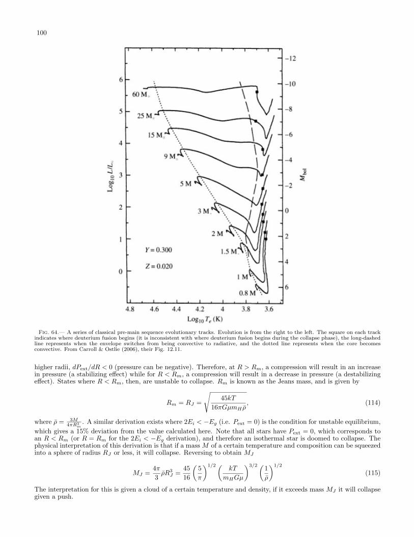
100

Fig. 64.— A series of classical pre-main sequence evolutionary tracks. Evolution is from the right to the left. The square on each trackindicates where deuterium fusion begins (it is inconsistent with where deuterium fusion begins during the collapse phase), the long-dashedline represents when the envelope switches from being convective to radiative, and the dotted line represents when the core becomesconvective. From Carroll & Ostlie (2006), their Fig. 12.11.

higher radii, dPext/dR < 0 (pressure can be negative). Therefore, at R > Rm, a compression will result in an increasein pressure (a stabilizing effect) while for R < Rm, a compression will result in a decrease in pressure (a destabilizingeffect). States where R < Rm, then, are unstable to collapse. Rm is known as the Jeans mass, and is given by

Rm = RJ =

√45kT

16πGµmH ρ, (114)

where ρ = 3M4πR3

m. A similar derivation exists where 2Ei < −Eg (i.e. Pext = 0) is the condition for unstable equilibrium,

which gives a 15% deviation from the value calculated here. Note that all stars have Pext = 0, which corresponds toan R < Rm (or R = Rm for the 2Ei < −Eg derivation), and therefore an isothermal star is doomed to collapse. Thephysical interpretation of this derivation is that if a mass M of a certain temperature and composition can be squeezedinto a sphere of radius RJ or less, it will collapse. Reversing to obtain MJ

MJ =4π

3ρR3

J =45

16

(5

π

)1/2(kT

mHGµ

)3/2(1

ρ

)1/2

(115)

The interpretation for this is given a cloud of a certain temperature and density, if it exceeds mass MJ it will collapsegiven a push.

101

3.13.3. What causes these overdensities?

In general, density perturbations in the ISM are caused by turbulence (Nguyen 2012). Turbulence can generated byany of the following: magnetorotational instability in galactic disks, spiral arm instabilities, accretion of extragalacticgas, colliding flows in molecular clouds, and expanding HII regions (Nguyen 2012).

3.13.4. Why do D and Li fusion occur before H fusion? Do they change this cycle?

Deuterium and lithium fusion both occur before stars reach the ZAMS. D burning was described above as occuringnear 2000 - 3000 K sometime during the accretion to homologous contraction transition phase. Li burning (both 6Liand 7Li have large cross-sections for proton capture) occurs at around 2 × 106 K, which is achieved just before theprimary H-burning nuclear processes begin to dominate (Nelson et al. 1993). Since there is very little of either elementin protostars, burning Li and D do not change significantly the overall evolution of protostars onto the main sequence.Objects destined to become brown dwarfs can actually burn D (for masses &0.013 M) and Li (&0.06 M), but doingso does not stop them from passing the degeneracy line and cooling.

3.13.5. How does fragmentation work?

Consider the Jeans mass, Eqn. 115, which is MJ ∝ T 3/2ρ−1/2. If the equation of state is isothermal, then MJ ∝ρ−1/2. If however the equation of state is adiabatic, then PV γ ∝ P 1−γT γ is a constant, giving P ∝ T 5/2, which,combined with P ∝ ρT (ideal gas law), gives us T ∝ ρ2/3 and MJ ∝ ρ1/2.

What this means is that during the initial collapse, the Jeans mass decreases (as it decreases with increasing density),allowing local regions of collapsing material to themselves collapse independently, leading to fragmentation of the cloud.Once the cloud becomes optically thick, however, fragmentation must end, since the Jeans mass now increases withdensity. A rudimentary means (Kippenhahn & Weigert 1994, pg. 254 - 255) of calculating the MJ at which thecloud collapses is to equate the energy loss rate (gravitational potential energy divided by the free fall time) with theStefan-Boltzmann law (since a blackbody maximizes the amount of light the object can emit). This gives us (assuminga 1000 K cloud at the time the system becomes optically thick) MJ is of order 1 M.

3.14. Question 15

QUESTION: Sketch the rotation curve for a typical spiral galaxy. Show that a flat rotation curveimplies the existence of a dark matter halo with a density profile that drops off as 1/r2.

If we approximate the movements of disk stars as circular and on the plane of the galactic disk, then uniform circularmotion gives (Schneider 2006, pg. 100 - 101)

v2(r) = GM(r)/r. (116)

If dark matter did not exist, we may use M(r) = Mlum and assume some mass to light ratio to convert surfacebrightness to mass. While the M/L can indeed be adjustable (one can either determine it by determining the stellarpopulation in a region of the galaxy and the finding the M/L from stellar evolution models, or simply use M/L as afitting parameter), the rotation curves of spiral galaxies are, at large r, flat, which is wholly incompatible with anyscaled M/L as we shall see below.

The dark matter can be determined by (Schneider 2006, pg. 100 - 101)

Mdark(r) =r

G(v2(r)− v2

lum(r)) (117)

Suppose mass is distributed in our galaxy with a ρ = A/r2 profile. From dM/dr = 4πr2ρdr, M(r) = 4πAr. Pluggingthis into Eqn. 116 gives us a flat velocity profile.

The reason this flat velocity curve implies the existence of dark matter is because observationally the rotation curveremains flat to as large an r as H i kinematics (Rmax = 30h−1 kpc) or satellite galaxy orbital statistics (Rmax = 100h−1

kpc) allow us to probe (Schneider 2006, pg. 101). Since for an 1/r2 density profile M ∝ r, the only thing limitingthe halo mass is the extent of the halo. This, however, is not the case for the density of stars in the galactic halo,which has ρ ∝ r−3.5. The stellar halo therefore has a definite maximum mass (assuming the central density is a finiteconstant) and cannot produce a flat velocity profile out to very large radii. We therefore must supplement luminousmatter with a large body of dark matter.

Fig. 65 shows a number of rotation curves for different spiral galaxies. The decomposition of the rotation curve ofNGC 3198 into a disk and halo component is not unique, and in this case it has been assumed that the entirety of theinnermost rotation curve is due to luminous matter (this is known as the “minimal mass halo”).

The innermost region of the rotation curve has velocity v ∝ r, indicating rigid body rotation due to a M(r) ∝ r3

(i.e. constant density). This suggests that the bulge and inner halo have a large constant mass density that dominatesover the mass contribution of the disk and dark matter halo (see Carroll & Ostlie (2006), pg. 919, Fig. 24.28).

102

Fig. 65.— Left: the rotation curves of a number of spiral galaxies, all of which asymptote to some roughly constant value at large radii.Right: the rotation curve of NGC 3198, and a decomposition of that curve into a disk and halo component assuming a minimal mass halo.From Schneider (2006), his Figs. 3.15 and 3.16.

Cosmological simulations by Navarro et al. (1996) give the following profile for a dark matter halo:

ρ(r) =ρ0

(r/a)(1 + r/a)2(118)

Despite no longer diverging because of the asymptote at the centre, the NFW profile is still divergent if r → ∞, andso an outer limit for the disk must be defined.

3.14.1. How do halo properties scale with the properties of luminous matter in late-type galaxies?

This information is from Schneider (2006). More luminous galaxies tend to have more massive halos. For thecharacteristic values of the various Hubble types, one finds vmax ∼ 300 km/s for Sa’s, vmax ∼ 175 km/s for Scs,whereas Irrs have a much lower vmax ∼ 70 km/s. Given the same overall luminosity, vmax is higher for earlier types ofspirals, reflecting an increase in bulge mass. The overall shape of the rotation curve does not change, indicating thatdark matter (with a common density profile) dominates spiral galaxy rotation curves after several kpc.

3.14.2. How do we observationally determine the rotational profiles of galaxies?

Observations of the rotation of our own Galaxy are done mostly by using long-wavelength (to sidestep extinction)gas tracers, or, with stars very close to the Sun, by measuring the Oort constants. In the region of the galaxy interiorof our own orbit, this can be done using the “tangent point” method if we assume orbits are circular (they should bedue to dissipation) - measuring maximum Doppler shift along one line of sight will give us the rotational velocity ofthe galaxy at one radius (see (Schneider 2006, pg. 62)). In the region exterior to our galaxy, this is mainly done bylooking at the radial velocity of objects with known distance measurements.

The rotation profiles of other galaxies are much easier to observe. Doppler shift observations of the H i disk and thestars, combined with inclination information obtained by disk inclination, allow us to probe the rotation profiles ofspirals and lencticulars. Early-type galaxies often lack an H i disk, and astronomers instead rely on observing stellarkinematics, and then binning large swaths of the galaxy together to increase signal-to-noise (integral field spectrographsare useful here, since they can create 2D spectral maps of the galaxy, which can then be binned). Alternatively, themotions of other objects, such as planetary nebulae and satellite galaxies, or the temperature of embedded hot gascan be used (Schneider 2006, pg. 101).

3.14.3. What is the difference between late and early type rotation curves?

While late-type galaxies get most of their pressure support from rotation, early-type galaxies obtain much of theirsupport from the velocity dispersion (equivalent to a “thermal pressure” in a gas). The observational means ofdetermining this support is absorption line spectroscopy in order to determine the line-of-sight velocity distribution(LOSVD), which can be written out as the velocity v, (Gaussian) dispersion σ and a series of Gauss-Hermite momentsstarting with h3.

A good first order measurement for the support against gravity is the RMS velocity vRMS =√v2 + σ2. Much like

spiral galaxies, the vRMS along the major axis of an early-type galaxy could be compared to the expected vRMS froma set (or fit-for) M/L and the surface brightness profile of the galaxy. vRMS, however, assumes that the absorptionline profile is a Gaussian, or, equivalently, that the distribution of stellar kinetic energies is isotropic. In general thisis not true, and results in the “mass-anisotropy degeneracy” (Binney & Merrifield 1998, pg. ). As an example (Fig.in Binney & Merrifield (1998)), let us define a cylindrical coordinate system for an early-type galaxy with z along the

galaxy’s minor axis. Suppose σ is greater along the θ direction than the r direction. An σ measurement of the lineof sight crossing the galactic centre would be sensitive to σr, but not σθ, while the reverse would be true for a line

103

TABLE 1Thermal phases of the ISM, from Table 1.3 of Draine (2011) with additional information from elsewhere in Draine and

from Ferriere (2001) and (Pogge 2011, Ch. 1). The total mass of hydrogen in the galaxy (R < 20 kpc) that is locked in theISM 4.9× 109 M, and the total mass of helium is 1.8× 109 M (Draine 2011, pg. 5). Ferriere (2001) gives slightly theslightly different number of 1× 1010 M (including He), though her mass fractions are similar. Molecular clouds is

separated by density into diffuse and dense H2 in Draine (2011). The fraction of the ISM that is in H i is 0.6 (Draine 2011,Table 1.2), and the CNM and WNM fractions are from (Draine 2011, pg. 331).

Phase Temperature(K)

Densitycm−3

fV fM Heating Mechanisms Cooling Mechanisms

Molecular clouds (H2) 10 - 50 102 - 106 0.001 0.17 Dust photoelectrons, cos-mic rays, starlight

Fine structure (especiallyCI), CO line emission

Cool H i (CNM) 100 30 0.01 0.24 Dust photoelectrons, cos-mic rays, starlight

Fine structure

Warm H i (WNM) ∼5000 0.6 0.4 0.36 Dust photoelectrons, cos-mic rays, starlight

Fine structure, opticallines

H ii (WIM) 104 0.3 - 104 0.1 0.23 forall H ii

H and He photoelectrons Optical lines, fine-structure, bremsstrahlung

H ii coronal gas (HIM) & 105.5 ∼ 0.004 ∼0.5 SN/stellar wind shock-heating

Adiabatic expansion, X-ray emission

of sight that crossed through the galactic outskirts. To break this degeneracy, the higher order h3 and h4 moments,which probe these anisotropies, must be fit for (Binney & Merrifield 1998, pg. ). To do this, however, requires goodS/N, and as a result extensive long-slit spectroscopy or integral field spectroscopy must be performed (Weijmans et al.2009).

3.15. Question 16

QUESTION: What thermal phases are postulated to exist in the interstellar medium? Describe thedominant mechanism of cooling for each phase.

Most of the information in this section comes from a combination of Draine (2011), (Pogge 2011, Ch. 1) and Ferriere(2001).

Interstellar matter accounts for ∼10 15% of the total mass of the Galactic disk. It tends to concentrate near theGalactic plane and along the spiral arms, while being very inhomogeneously distributed at small scales. Roughly halfthe interstellar mass is conned to discrete clouds occupying only ∼1 2% of the interstellar volume. These interstellarclouds can be divided into three types: the dark clouds, which are essentially made of very cold (T ≈ 10 20 K) moleculargas and block off the light from background stars, the diffuse clouds, which consist of cold (T ≈ 100 K) atomic gas andare almost transparent to the background starlight, except at a number of specic wavelengths where they give rise toabsorption lines, and the translucent clouds, which contain molecular and atomic gases and have intermediate visualextinctions. The rest of the interstellar matter, spread out between the clouds, exists in three different forms: warm(mostly neutral) atomic, warm ionized, and hot ionized, where warm refers to a temperature of ∼ 104 K and hot atemperature of ∼ 106 K.

Mixed in with all but the very hottest phases is interstellar dust. Dust grains are an important source of interstellarextinction, gas-phase element depletion, sites of interstellar chemistry, etc. This is solid-phase rather than gas-phasematerial. Dust grains range in size from a few microns down to macromolecular scales (clumps of 50 - 100 atoms orless).

The interstellar medium is in general not in any sort of thermal equilibrium. Nevertheless, it can be classifiedinto a number of different thermal phases, characterized by differing thermodynamic properties. A summary of theseproperties can be found in Table. 1. Draine also cites “cold stellar outflows” as a component of the ISM, but this isnot echoed in the other two works.

The temperature of the ISM is given by the Maxwellian distribution of velocities established by ISM gas and dustparticles colliding elastically with one another (this is known as the “kinetic temperature”, distinguishable from theeffective temperature obtained by observing line strengths when the ISM is not in LTE) (Pogge 2011, Ch. 1). Sincekinetic energy is distinct from internal energy, in order to [gain/lose] energy the ISM must [absorb/emit] a photon,[followed by/preceded by] a collisional [de-excitation/excitation] to bring a particle [out of/into] an excited state.In this manner, the kinetic energy is coupled with the internal energy and therefore the radiation field. In localthermodynamic equilibrium (LTE), the radiation field is completely coupled to the matter, meaning that a singletemperature can describe them both. In non-LTE (i.e. low-density) conditions, the distribution of excited states isgoverned by collision and radiative rates, and may either be described by departure coefficients nstate/n(LTE)state orby an “excitation temperature”. An extreme example of a non-thermal distribution of excited states is an invertedpopulation, which may exist due to optical or collisional pumping, and produces a maser or laser from stimulatedemission.

Which cooling mechanisms dominate, therefore, is dependent on which process:

104

• Collide frequently

• Results easily in excited states

• Can be reached at the medium’s particular kinetic temperature

• Results in photon emision before collisional de-excitation

• Emits a photon that can most easily escape the system

3.15.1. Molecular Gas

Diffuse molecular gas is similar to the cool H i clouds, but with sufficiently large densities and column densitiesso that H2 self-shielding allows molecules to be abundant in the cloud interior. Dense molecular gas is composedof gravitationally bound clouds that have achieved nH & 103 cm3 . These clouds are often “dark” - with visualextinction AV & 3 mag through their central regions. In these dark clouds, the dust grains are often coated with“mantles” composed of H2O and other molecular ices. It is within these regions that star formation takes place. Itshould be noted that the gas pressures in these “dense” clouds would qualify as ultrahigh vacuum in a terrestriallaboratory.

Molecular gas is primarily composed of H2, but H2 is not directly observable in the radio 20; this feature of H2

emission is also what prevents it from being a good coolant. Instead CO rovibrational line emission (particularly 2.6mm) acts as the primary tracer.

As noted in Question 3.5, the primary means of cooling for an H2 region is C+ fine structure line emission at lowdensities and reasonably high temperatures (∆E/k for the transition is 92 K, or 168 µm). At other densities andtemperatures, CO rovibrational line emission contributes the majority of cooling.

Photodissociation Regions (PDRs) are the warm, partially ionized surfaces of molecular clouds. The UV radiationfield impinging upon the cloud may be either a discrete UV source, like O or B stars, or the diffuse interstellar radiationfield (ISRF). The principal ionic state in a PDR is C+, which is why they are sometimes referred to as “C+” or “C II”regions. They get their name from the fact that this is the region in which H2 is dissociated by UV photons into H i.Since dust and molecular gas are closely related (much of the dust in the Galaxy is in molecular clouds, since significantshielding is required for both to exist (Glover & Clark 2012)), PDRs are also significant sources of FIR emission fromhot dust. PDRs are heated by photoelectric heating from dust grains and UV emissions from the interstellar radiationbackground. They are cooled by emission of collisionally excited FIR fine structure lines, including C+ or [C II] (158µm) and [O I] (63 µm), CO rovibrational transitions, collisionally excited NIR H2 rovibrational lines and collision ofmolecules with dust grains. If the surface of the PDR is hot enough to be partially ionized, NIR/optical lines frompartially ionized metals will also contribute.

3.15.2. Cold Neutral Medium

Cold neutral hydrogen (H i) gas is distributed in sheets and filaments occupying by volume ∼1 - 4% of the ISM withtemperatures of ∼80 - 100 K and densities of ∼30 - 50 cm−3. The main tracers are UV and optical absorption linesseen towards bright stars or quasars, and 21 cm line emission (and absorption if a bright object is in the background).Indeed, mapping of the 21-line emission works to pick out both the warm and cold neutral medium: narrow peaksseen in both emission and absorption are due to the CNM, while broader features seen in emission only are due to theWNM. The CNM is approximately in pressure equilibrium with its surroundings.

Cooling is accomplished primarily through the [C II] (158 µm) fine structure transition, and from the [O I] (63 µm)fine structure transition at higher temperatures (see Fig. 66). The critical densities for [C II] and [O I] are ∼ 4× 103

cm3 and ∼ 105 cm3, respectively, implying that collisional deexcitation of these levels is unimportant in the diffuseISM of the Milky Way.

3.15.3. Warm Neutral Medium

Warm neutral atomic hydrogen occupies ∼ 30 − 40 % of the volume of the ISM, and is located mainly in pho-todissociation regions on the boundaries of HII regions and molecular clouds. It has characteristic temperatures of∼5000K and densities of ∼0.5 cm−3 and is traced by H i 21-cm line emission. The WNM is approximately in pressureequilibrium with its surroundings.

WNM cooling is generally the same as CNM cooling. In the 1000 K range of temperatures [O I] emission generallyis a better coolant than [C II]. As 104 K is approached, H atom excited states become populated, and Ly α becomesa significant coolant.

3.15.4. Warm Ionized Medium

Diffuse gas with temperatures of 6000 - 12000 K, and densities ∼ 0.1 cm−3, occupying about ∼ 10 - 25 % of thevolume of the ISM. While primarily photoionized (it requires about 1/6th of all of the ionizing photons emitted by theGalaxy’s O and B stars), there is some evidence of shock or collisional ionization high above the plane of the Galaxy.

20 It can be detected as absorption lines in the UV/optical, but extinction in dense molecular clouds prevents this from being a usefulprobe (Ferriere 2001).

105

Fig. 66.— An H i cooling curve for nH = 0.6 cm−3 and ne/nH = 1.7× 10−2. From Draine (2011), his Fig. 30.1.

It is traced by low-surface brightness Hα (6563 A) emission. Nearly 90 % of the H+ in the Galaxy resides in the WIM,with the remaining 10 % in the bright high-density H ii regions that occupy a tiny fraction of the ISM. The WIM isassociated with regions of recent massive-star formation and planetary nebulae (the ejected outer envelopes of AGBstars photoionized by the cooling WDs at their centres).

The UV, visible and IR spectra of H ii regions are very rich in emission lines, primarily collisionally excited lines ofmetal ions and recombination lines of H and He. H ii regions are also observed at radio wavelengths, emitting radiofree-free emission from thermalized electrons and radio recombination lines from highly excited states of H, He, andsome metals.

The WIM cools through recombination radiation, where an electron recombines with an ion and therefore no longercontributes its kinetic energy to the medium, and free-free emission, where free electrons accelerate off of each otherto produce bremmstrahlung. Most importantly, however, metal-polluted H ii regions are generally at temperatures atwhich metals such as O may be collisionally excited (this is difficult to achieve with He or He+, as their first excitedstates are highly energetic). Table 27.2 of Draine lists principal collisionally excited lines. In metal-depleted H iiregions (0.1 × the metallicity of the Orion Nebula) the cooling rate from collisionally excited (forbidden) line emissionis several times larger than the radiative recombination and free-free rates (which are roughly comparable). For anOrion-metallicity cloud it is about an order of magnitude.

The balance between heating and cooling provides, given a certain density, the temperature of an H ii region. InH ii regions photoionization provides the primary means of heating the gas, and balancing that against the coolingmechanisms described above, and assuming nH = 4000 cm−3 nets us ∼8000 K.

3.15.5. Hot Ionized Medium (Coronal Gas)

Hot, low-density gas heated by supernovae, with temperatures > 105.5 K and very low densities of < 0.004 cm−3

occupy ∼50 % of the ISM. The vertical scale height of this gas is ∼3 kpc or larger, so it is sometimes referred to in theliterature as the hot corona of the galaxy. This hot gas is often buoyant and appears as bubbles and fountains highabove the disk. Its primary tracers are absorption lines seen towards hot stars in the far-UV (e.g., O IV, N V, and CIV) in gas with T ≈ 105 K, and diffuse soft X-ray emission from gas hotter than 106 K.

Coronal gas is primarily heated and collisionally ionized by the violent interaction between the ISM and rapidlyexpanding gas from supernovae. At high temperatures, Compton heating becomes important as well. Coronal gascooling is dominated by neutral H and He collisional excitation, with collisional excitation of He+ becoming importantat 4× 105 K. UV collisionally excited lines (mainly forbidden lines at lower and allowed lines at higher temperatures)also play a role. At extremely high temperatures, free-free continuum radiation, appearing at EUV and soft X-rayenergies, dominates.

3.15.6. Why Do the Phases of the ISM Have Characteristic Values At All?

Simply put, phases of the ISM exist when the various phenomena that affect ISM temperature and density balanceout and form a stable equilibrium. H ii regions, for example, only exist in the vicinity of a strong UV source, such asa young cluster or association. Molecular hydrogen, on the other hand, can only form in regions of high self-shielding,where the amount of dissociation radiation and heating are minimized.

As an example, consider the Two-Phase Model for describing why there is a warm and cold neutral medium (pg.341 - 343 of Draine and Ch. 1 of Pogge). The generalized loss function L is defined as the net cooling subtracted by

106

the net heating per unit volume. We may calculate equilibria between heating and loss (L = 0) given some averagedensity of the medium and the need to exert a certain pressure. At this equilibrium, if ∂L/∂S < 0, the equilibrium isunstable (heating is an increase in entropy, and so if ∂L/∂S > 0 entropy is increased for some reason, the net coolingeffect will, over time, bring the system back to equilibrium).

Fig. 67.— Steady state temperature as a function of thermal pressure. Since p is proportional to the inverse of Γ/nT , left of the line,Λ < Γ/nT the system will heat up until it reaches equilibrium, and right of the line Λ > Γ/nT resulting in net cooling - the directionof heating/cooling is shown by the vertical arrows. Either a temperature or a pressure perturbation in the dashed-line region results inmovement away from the equilibrium. From Draine (2011), his Fig. 30.2.

Suppose loss is due to collisionally excited line emission. Then L = n2Λ − nΓ (Λ is cooling from collisions, Γ isheating). Fixing nT for an ideal gas means fixing the pressure, and for both dust photoions and cosmic rays Γ isindependent of the ISM properties, for a given p, i.e. a given nT , we can find the temperature at which Λ = Γ/nT(Pogge, Ch. 1, pg. 21). Therefore the heating/cooling balance can also be plotted in pressure-temperature space(another way of putting it is that given a pressure p, we find equilibria points). This is plotted in Fig. 67. As notedin the figure caption, the dashed-line region represents an unstable equilibrium, resulting in two unjoined regions ofequilibrium - hence, a two-phase ISM.

The fact that more than two phases exist in reality is a reflection of the fact that additional physics must be included,such as H2 grain catalysis and H i ionization. The standard picture of the ISM is a three-phase model (where coldincludes molecular clouds and warm includes H ii regions) - the hot phase is the coronal gas, shock heated by SNebubbles, though this model is likely an oversimplification. See Ch. 1, pg. 23 - 24 of Pogge for details.

3.16. Question 17

QUESTION: Characterize the stellar populations in the following regions: i) the Galactic bulge ii) theGalactic disk, outside of star clusters iii) open star clusters iv) globular clusters v) a typical ellipticalgalaxy.

Unless otherwise noted, the information in this section comes from Carroll & Ostlie (2006), Ch. 24.2 and Schneider(2006), Ch. 2.3. Information on open clusters comes mainly from Binney & Merrifield (1998), Ch. 6.2.

Table 24.1 neatly summarizes much of the information required for this question. It is reproduced here as Fig. 68.

3.16.1. The Galactic Disk

The disk is roughly 40 - 50 kpc in diameter, with an ellipticity of about 0.9. It is composed of two major components.The younger think disk has a scale height of ∼350 pc and contains star formation regions. The thin disk dust and

107

Fig. 68.— Properties of different components of the Milky Way. From Carroll & Ostlie (2006), their Table 24.1.

H2 gas lane (sometimes called the “young thin disk”) has a scale height of ∼90 pc, while H i has a scale height rangefrom 160 to 900 pc depending on distance from the centre of the galaxy. The less well-defined thick disk likely has ascale height of ∼1000 pc and is an order of magnitude less dense than the thick disk. Combined, the two disks haveroughly the following profile:

n(z,R) = n0(e−z/350 + 0.085e−z/1000)e−R/hR (119)

where all values are in pc and hR, the disk scale height, is > 2.25× 103 pc.As a general rule, thick disk stars are more metal poor than thin disk stars. Popular means of measuring metals

include Z, the mass fraction of the star composed of elements heavier than He, and the metallicity, [Fe/H], defined as

[Fe/H] = log10

[(NFe/NH)star

(NFe/NH)

]. (120)

Metallcity values in our galaxy range from 0.6 to -5.4, and more negative numbers generally represent older stars,though as noted in Sec. 3.7 significant challenges exist in relating metallicity to stellar age. The metallicity range inthe thin disk is from -0.5 to 0.3, and in the thick disk from about -0.6 to -0.4, though the dispersion is higher. Thissuggests the thin disk began forming about 8 Gyr ago, while the thick disk formed 10 - 11 Gyr ago.

Spiral arms are associated with the thin disk (since they form out of star-forming regions in the young thin disk).As a result, young OB associations are associated with the thin disk, and die before they become part of the thickdisk.

3.16.2. The Galactic Bulge

The galactic bulge occupies the innermost ∼0.7 kpc of the galaxy, and has a scale height of 100 - 500 pc, dependingon the age of the stellar population being measured. Its light follows roughly a Sersic profile of index 4, i.e. a de

108

Vaucouleurs profile:

I(R) = Ie exp(−7.669((R/Re)1/4 − 1)) (121)

where Ie is the intensity at Re, the radius enclosing half of the light from the bulge. Integrating I(R) gives us therelation L = 7.215πIeR

2e.

The chemical enrichment of the bulge is strange: the range of metallicities ranges from -2 to 0.5, and suggest threedistinct stellar populations: one with age just 200 Myr, another between 200 Myr and 7 Gyr, and a third older than 7Gyr. The age-metallicity relation works in reverse, however - the most metal-rich stars are also the oldest, while theyoungest stars have a range of metallicities. This may be due to rapid enrichment of the bulge through CC SNe earlyin its life combined with metal-poor gas inflow later in the evolution of the bulge. It is also possible that some metalrich stars are actually members of the inner galactic disk.

A bar extends outward from the bulge, and is responsible for perturbing the 3-kpc spiral arm outward.

3.16.3. Open Star Clusters

Open clusters are coeval21 groups of stars that form out of a single giant molecular cloud. They are distributed closeto the galactic thin disk. They consist of anywhere between a few to several thousand stars, with a spatial extent ofseveral pc and a density ranging from 0.1 to 103 pc−3 (very low-density open clusters are known as “associations”).Unlike globular clusters, they do not have “simple”, well-ordered structures, though King density profiles (see below)can provide reasonable fits. The relaxation time for open clusters is small enough that most older clusters are expectedto be thermalized. Some evidence of this exists in the form of observations of mass segregation (if all objects havethe same energy, more massive objects will have lower characteristic velocities and sink to the centre of the potential),though direct measurements of stellar kinematics contradict these observations (see Binney & Merrifield, pg. 388 -389).

Open clusters often contain significant amounts of ISM gas and dust, as well as a population of hot, blue stars, bothindicators of the youth of the average open cluster. The distribution of known open cluster ages peaks at ∼100 Myrand drops off sharply, though a few open clusters > 3 Gyr or older have been observed. Metallicity is generally aroundsolar, but older clusters may be as metal poor as [Fe/H] ≈ -0.75 and younger cluster as rich as [Fe/H] ≈ 0.25.

Open cluster lifetimes are limited by close encounters with GMCs - only rich, densely populated clusters (which havesignificant gravitational potentials) and clusters born on the upper and lower fringes of the thin disk (where there arefew GMCs) may avoid tidal destruction.

Since kinematic parallax can be used to determine their distance, and their stellar populations are coeval and fairlyyoung, they (like their globular cluster cousins) are useful laboratories for stellar evolution.

3.16.4. Globular Clusters

The globular cluster system is connected to the Galactic halo. Stellar members of the halo are distinguished frommembers of the disk by a high velocity component perpendicular to the plane of the disk. As a whole, this galactichalo can be represented by either a density profile of

n(r) = n0(r/a)−3.5 (122)

where n0 = 4 × 10−5 pc−3 (roughly 0.2% of the thin disk’s midplane value) and a ∼ 1000 pc. Halo field stars havebeen found as far as 50 kpc away, while GCs arguably extend out to 120 kpc. It is not clear whether or not the fieldstars and GCs form a unified population of halo members, as there is some evidence to suggest that the field starsoccupy a flattened volume with c/a ∼ 0.6, rather than the spherical volume occupied by GCs.

Globular clusters (GCs) are compact (∼ 10 pc), highly spherical (b/a ∼ 0.9) collections of 105 - 106 metal-poorstars. GCs have a King density profile (an isothermal sphere with a fast drop-off to keep total mass finite; Binney &Tremaine, pg. 307 - 308), and the core stellar densities of GCs can be massive, up to 1000 pc−3. Because they are oldand coeval, most of the more massive stars have already evolved off the main sequence; from isochronal fitting of this“main sequence turnoff”, GCs have an age range from 11 - 13 Gyr. The & 150 GCs of our Milky Way come in twodifferent populations: the metal poor population ([Fe/H] < - 0.8) is spherically distributed, while the more metal richpopulation ([Fe/H] > - 0.8), with the notable exception of 47 Tucana, is primarily distributed near the galactic thickdisk, and may actually be associated with it (both populations having a scale height of 1 kpc and similar rotationsabout the galactic centre). GCs can be found from 500 pc to 120 kpc from the galactic centre, though the majority ofthem are within 40 kpc of the galactic centre. It is debatable whether or not GCs past 70 kpc were actually formedalongside the MW, or were captured from, or formed out of, satellite galaxies.

3.16.5. (Ordinary) Elliptical Galaxies

Ordinary elliptical galaxies, at least to first order, resemble the bulges of spiral galaxies. Their brightness profileis well-described by the de Vaucouleurs profile (Eqn. 121). Their total mass ranges from 108 - 1013 M and their

21 Open clusters are young enough that they cannot be considered purely coeval. A commonly observed mismatch between the age ofthe cluster as determined by the main sequence turnoff and as determined by low mass protostar cooling suggests low-mass stars formearlier than high-mass stars (Binney & Merrifield 1998, pg. 384).

109

physical extent ranges from 1 - 100 kpc (Carroll & Ostlie 2006, pg. 985). The stellar population in an average ellipticalis red, and little (but non-zero) mass in gas and dust. Ellipticals hold their shape by velocity dispersion anisotropyrather than bulk rotational velocity - more orbits are oriented along the elliptical’s shortest axis than along ather axes.While thermalization of the stellar population will lead to a roundening of the system (ex. with globular clusters), therelaxation times of ellipticals are an order of magnitude greater than their age. For lower mass ellipticals, rotationalsupport due to an overall galactic spin also plays a significant role (these ellipticals also have more “disky” isophotes).

The centres of elliptical galaxies have redder stellar populations than their outskirts, suggesting either that metallicityis highest at the centre, or that the central stellar population is older22 (Schneider 2006; Binney & Merrifield 1998,pgs. 193, 320). The same issue confounds our ability to determine an absolute metallicity for ellipticals. Efforts todisentangle the two effects have lead to the determination that most ellipticals formed their stars at z & 2 - 3 in aperiod of star formation inversely proportional to the mass of the galaxy (the most massive galaxies formed their starsin . 1 Gyr) (Renzini 2006).

3.16.6. What do these properties tell us about the formation and evolution of these objects?

This information comes from Ch. 26.2 of Carroll & Ostlie (2006).The earliest attempt at explaining the properties of these different regions of the MW, and other large late-type

galaxies, was the Eggen/Lynden-Bell/Sandage homologous collapse model, where a massive proto-galactic cloud col-lapsed to form a single galaxy. In this model, the oldest (pop II) halo stars were formed when the cloud was nearlyspherical and collapsing radially, which explains their current trajectories. The younger disk stars were formed afterthe kinetic energy of the infalling cloud was dissipated through thermalization of the cloud constituents, followed byradiation. This process is spherically symmetric, and therefore no angular momentum is lost; this angular momentuminstead generates a disk. This disk is metal enhanced from the first generation of stars that exploded back during theperiod of radial collapse, and so new stars formed after disk formation are metal rich.

This model fails to explain a number of features of our galaxy: first, the halo has no sense of rotation at all (whilethe homologous collapse model posts the cloud as having some initial angular momentum). The spread of ages in thehalo population is about 2 Gyr, an order of magnitude longer than the free-fall time of a giant proto-galactic cloud.Homologous collapse also would not explain a multi-component disk with varying ages.

The modern conception of the formation of an MW-like galaxy combines the homologous collapse model with abottom-up process of gas-rich mergers. Following inflation, a series of (dark and baryonic) matter-energy overdensitiesformed that were bottom-heavy, i.e. 106 - 108 M overdensities were much more common than 1010 M overdensities.Following recombination, these overdensities began to attract one another while gas began to fall into the potentialsof these overdensities. The initial collapse of these gas clouds (first on a free-fall timescale and then on a dissipativetimescale) generated the first stars and clusters, and the first dwarf galaxies were born. The degree of star formationwas different for different overdensities, so each dwarf galaxy had its own chemical history. As fragments combined toform larger galaxies, many of these dwarf galaxies were tidally destroyed, possibly leaving globular clusters that wereat their cores. The stars and clusters form the modern-day halo of massive galaxies. At the centre of the budding,the potential well is deepest, and as a result significant chemical processing occurred, a possible explanation for themetal-rich stars in the MW bulge. The globular cluster mass distribution was also formed out of the merging process- massive GCs were towed into the bulge through dynamical friction, while lightweight GCs were destroyed throughtidal disruption. Since there does not need to be any global sense of spin in the initial grouping of overdensities, thenet angular momentum of the halo is negligible. Not all the overdensities merge with the galactic DM halo within aHubble time, and the MW today features an extensive collection of dSph galaxies around it.

Since the relaxation time for stellar systems far exceeds the dissipation time for gas, the halo stars achieved fixedorbits (which they retain today), while the gas collapsed onto a thick disk with a temperature of ∼ 106 K. A burstof star formation followed, which simultaneously polluted the ISM from [Fe/H] < -5.4 to [Fe/H] ≈ -0.5 and generatedfeedback to prevent further star formation. (An alternate theory postulates that the thick disk of our MW was actuallyformed cold, but a major collision with another galaxy 10 Gyr ago puffed up the disk.) The gas continued to dissipateand form new stars. Stars forming out of the thin disk provided some feedback, but as gas was depleted from theISM, star formation slowed, and dissipation exceeded energy injection from feedback. The disk scale height eventuallyachieved the present-day scale height of the young thin disk.

Mergers continued after the formation of the galactic disk. New material streaming into the bulge from dwarfgalaxies, or kicked into the bulge due to bar instabilities, generated new populations of metal-poor stars.

Ellipticals are believed to have formed in one of two ways: either through rapid star formation (the overdensities formstars so quickly that little gas remains by the time they merge to form the dark matter halo) or through major mergersof late-type galaxies. The latter hypothesis has support from N-body simulations and observed stellar kinematics, andneatly explains the morphology-density relation (elliptical galaxies are preferentially found near the centres of clusters).At the same time, however, it is possible that deep potential wells favour rapid star formation (and independentlyalso favour clustering), and it is difficult to reconcile the existence of ellipticals with extensive globular cluster systemswith the merger picture (unless those GCs are the result of the major merger, or subsequent minor merger).

3.17. Question 18

22 This is known as the age-metallicity degeneracy, and is quantitatively given by Worthey (1994) as d ln td lnZ colours

≈ − 32

.

110

QUESTION: How can you determine the temperature of an H ii region?

Most of the information in this section comes from (Draine 2011, Ch. 18).There are three primary methods of determining the temperature of an H ii region: nebular line diagonstics, the

recombination continuum and dielectric recombination lines.Line diagnostics use ions with two excited levels that are both “energetically accessible” at the temperatures of

interest, but with an energy difference between them that is comparable to kT , so that the populations of these levelsare sensitive to the gas temperature. The level populations are normally observed by their line emission.

Line diagnostics are also useful for determining the density of an H ii region. To do this, ions with two or more“energetically accessible” energy levels that are at nearly the same energy are used, so that the relative rates forpopulating these levels by collisions are nearly independent of temperature. The ratio of the level populations willhave one value in the low-density limit, where every collisional excitation is followed by spontaneous radiative decay,and another value in the high-density limit, where the levels are populated in proportion to their degeneracies. Ifthe relative level populations in these two limits differ (as, in general, they will), then the relative level populations(determined from observed emission line ratios) can be used to determine the density in the emitting region.

During recombination, atoms with EK ≥ 0 become bound, meaning that the recombination continuum will peri-odically contain sharp drops, corresponding to the energy released when EK = 0 electrons become bound (they aredrops because EK < 0 free electrons do not exist). The strength of the jump is related to the population of negligibleKE electrons, and therefore is a function of the cloud density and temperature, or, more precisely, a function of theemission measure23 multiplied by T−3/2. To remove the emission measure dependence, we may use a recombinationline as scaling, so long as the line has a different temperature dependence than the amplitude of the drop. For example,the drop most commonly used to measure temperature is the “Balmer jump” at λ = 3645.1 A24. We can scale it withthe n = 11→ 2 (λ = 3769.7 A) hydrogen recombination line, which is proportional to the rate of recombination ontolevels n ≥ 11, which turns out to be ∝ EM × T−0.8. The ratio between the two measurements is ∝ T−0.7.

For some ions, it is possible to observe both collisionally excited lines and lines emitted following dielectronicrecombination 25. For example, electrons colliding with C IV can produce collisionally excited levels of C IV, butcan also produce excited levels of C III by dielectronic recombination. Because the rate coefficients for collisionalexcitation and for dielectronic recombination will have different temperature dependences, the ratio of dielectroniclines to collisionally excited lines will be temperature-sensitive, and therefore useful as a temperature diagnostic.Examples of useful line ratios are C III 2297/C IV 1549 A, O II 4705/O III] 1665 A, and C II 4267/C III] 1909 A.

3.17.1. Details?

Like hydrogen, a unified spin state for a multi-electron ion can be written in the form

2S+1LJ (123)

where S is the vector sum of the spin angular momenta and L the vector sum of the orbital angular momenta of allvalence electrons, and J = L+S . L is often written in SPDF notation (i.e. S is L = 0, P is L = 1, and so on) (Wood2011). Since these are conglomerate spins, there is no real reason that P must be higher energy than S, and so forth26.

Atoms or ions with six electrons have 2p2 as their lowest configuration. Their ground state is 3P, and the first twoexcited states are 1D and 1S. So long as the 1S term is sufficiently populated (which occurs when E/k . 7×104 K andthe ion is sufficiently abundant), then there will be observable emission from both excited states. Since these levelsare at very different energies, different temperatures will affect how the different states are populated. For example,consider the ion N II in Fig. 69, and assume that densities are below the critical density for both excited states. Inthis case, most N II ions are in their ground state, and as soon as a collision excites an electron, it will radiativelydecay back to the ground state. The power going from state 4 to 3 is E43n0C04

A43

A43+A41, while the power going from

state 3 to 2 is E32

(n0C03 + n0C04

A43

A43+A41

)A32

A32+A31. The collisional excitation rate Clu ∝ Ωlu

gle−Eul/kT , where Ωlu is

the (roughly of order unity and weakly dependent on temperature) collision strength and gl is the degeneracy of state

23 The emission measure EM ≡[

nenpκfree−free,ν

]Tτν is a measure of the column density of the cloud, scaled to how well it absorbs radiation

(Draine 2011, pg. 96).24 The inverse of the Balmer jump can be used to determine the temperature of stellar atmospheres - because ionization of n = 2 electrons

becomes possible with any photon with λ < 3647 A, there is a sharp drop in the spectrum of stars at that wavelength. The magnitude ofthis drop is dependent on the number of n = 2 excited hydrogen atoms, which, since the stellar atmosphere is in LTE, is dependent on theBoltzmann equation, and therefore the temperature (Carroll & Ostlie 2006, pg. 247).

25 Dielectronic recombination occurs when a free electron approaches an ion that contains one or more valence electrons. Instead ofinitiating a radiative recombination, the free electron transfers energy to one of the bound electrons, promoting the bound electron to anexcited state and losing enough energy to become bound to the ion. The two excited electrons can then drop to the ground state, orexchange energy to re-ionize one of them. See (Draine 2011, pg. 151 - 153).

26 For alkali atoms/ions, L and S individually do not contribute any changes in energy - the most prominent correction to the n-governedenergy level is fine splitting, caused by a relativistic correction and spin-orbit coupling (J)

111

l. As a result, the ratio of line emission power is

j4→3

j3→2∝ e−E43/kT

1 +Xe−E43/kT(124)

where X = A43Ω04

(A43+A41)Ω03, and there is an obvious dependence on temperature. See pg. 205 of Draine for details. Fig.

70 shows the line ratio as a function of temperature and density.Candidate 2p2 ions are C I, N II, O III, F IV, Ne V, and so on. C I is easily photoionized, and will have very low

abundance in an H II region. The ionization potentials of F IV, Ne V, and so on exceed 54.4 eV, and we do not expectsuch high ionization stages to be abundant in H II regions excited by main-sequence stars with effective temperatureskTeff ¡ 5 eV. This leaves N II and O III as the only 2p2 ions that will be available in normal H II regions. The samesituation exists for 2p4 ions and above (O I, F II, and Ne III being appropriate temperature diagonstics for 2p4, P IIand S III 3p2, and Cl II, Ar III, and K IV 3p4). Atoms/ions with seven (O II, F III, and Ne IV are usually used) andfifteen (S II, Cl III, and Ar IV are usually used) electrons have different energy levels, but the same principle applies.

Fig. 69.— Energy level diagram for temperature diagnostic 2p2 ion N II. From Draine (2011), his Fig. 18.1.

Note that it is assumed collisional excitation is the only way to achieve an excited state. This is not true if asubstantial contributor of excited states comes from recombination from the next ionized state.

3.17.2. How is density determined?

Density can be determined through collisionally excited optical/UV lines or near/far-IR fine structure lines.Ions with 7 or 15 electrons have 2s22p3 and 3s23p3 configurations, with energy-level structures that make them

suitable for use as density diagnostics: the ground state is a singlet 4S3/2 , and the first excited term is a doublet2Do

3/2,5/2. Let us consider OII (Fig. 71) and again assume low densities, so that a radiative decay immediately follows

from a collisional excitation. The relative intensity of the 2 → 0 and 1 → 0 lines (3727.1 and 3729.8 A; see Fig. 71)are, at low density

j2→0

j1→0=

Ω20

Ω10

E20

E10e−E21/kT ≈ Ω20

Ω10(125)

where the approximation comes from the fact that the fine-splitting energy is tiny, i.e. E21 kT . At high densities,the levels are thermalized (LTE), meaning

j2→0

j1→0=g2

g1

E20A20

E10A10e−E21/kT ≈ g2

g1

A20

A10. (126)

These two expressions involve fundamentally different microphysics, and as a result have different values. The sensi-tivity range for the diagnostic is the transition between the low density to LTE regime, which usually spans an orderof magnitude below to the same order of magnitude as the critical density.

112

Fig. 70.— Line ratio as a function of temperature for temperature diagnostic 2p2 ion N II’s 5756.2 and 6585.3 Alines. This is thecharacteristic shape of a temperature line diagnostic. From Draine (2011), his Fig. 18.2.

Fig. 71.— First five energy levels of the 2p3 ion O II. Of interest are the 2 → 0 and 1 → 0 (3727.1 and 3729.8 A) lines, which can beused as a density diagnostic. From Draine (2011), his Fig. 18.3.

Ions with triplet ground states - in particular, the 3P0,1,2 terms for np2 and np4 configurations - allow densitydetermination from the ratios of mid-infrared and far-infrared fine-structure lines. Examples are the 2p2 ions N II,OIII, and Ne V, the 2p4 ion Ne III and the 3p2 ion S III. If we treat the system as a three-level system (i.e. we do not

care about decays from higher energy states), the intensity ratio j2→1

j1→0has to first order no temperature dependence so

113

long as Eul kT , which is the case here (we need not worry about 2→ 0 transitions because ∆J = 2 is a forbiddentransition).

In both cases, collisional de-excitation of ions is dominated by electronion collisions, with rates that scale asneΩij/

√Te (“e” stands for electron). If the collision strengths Ωij were independent of temperature, and the electron

temperature is sufficiently high that E21/kTe, the line ratio would be dependent solely on ne/√Te, and a plot of the

line ratio vs. ne/√Te would bridge the low and high density extremes in the manner shown in Fig. 72. This is often

not the case, and there is some dependence on Te as well.

Fig. 72.— [S III] 33.48 µm / [S III] 18.71 µm as a function of ne/√Te and Te. This is the characteristic shape of a density line diagnostic.

From Draine (2011), his Fig. 18.6.

Densities can also be determined using the “Balmer decrement” (the set of ratios that includes Hβ to Hα emission,Hγ to Hβ emission, and so on). At low densities these ratios are used to measure extinction, but at high densities theline ratios are affected by collisional effects, with systematic enhancement of the high-n levels relative to Hα and Hβ,and these line ratios can therefore be used to constrain the electron density when ne > 104 cm3.

3.17.3. How is abundance determined?

The abundance of He relative to H is determined from comparison of the strengths of radiative recombination lines ofH and He in regions ionized by stars that are sufficiently hot (Teff > 3.9× 104 K) so that the He is ionized throughoutthe H ii zone. The abundances relative to H of elements heavier than He can be inferred by comparing the strengths ofemission lines excited by collisions between electrons and ions heavier than He to emission resulting from recombinationof electrons with H+, since the former is dependent on the density of these ions, while the latter is dependent on thedensity of H+. There generally is also a significant dependence on temperature, which must be determined separately.Fine-structure lines can also be used to determine abundances of ions with fine-structure splitting of the ground state.

To determine the total abundance, one must sum over all important ion stages. In an H ii region ionized by a B0star, most of the oxygen will be O II, because there will be few photons above the O II→ O III ionization threshold of35.1 eV. However, in H ii regions ionized by hotter stars, or in planetary nebulae, much of the oxygen may be presentas O III.

Optical recombination lines resulting from radiative recombination of X+r+1 have similar temperature and elec-tron density dependencies as H+ recombination lines. The ratios of these lines, therefore, are a probe of elementalabundances that is not highly dependent on temperature.

3.17.4. Can you use the same techniques to determine the properties of other ISM regions?

It is difficult to determine properties of the ionized medium that are beyond the effective ranges of particular nebulardiagnostics, as described above. Use of different species may help widen this range, but it is still theoretically possibleto have an H ii region that is too dense, for example, for diagonostics to probe.

H2 itself does not have line emission at the temperatures and densities found in the ISM, but embedded CO does,and the ratio of peak intensities of CO lines can be used to determine the temperature of the cloud (Ferriere 2001,pg. 1037). The low-J levels are very optically thick SO HOW DO THEY CONTRIBUTE TO COOLING?, and if thelines are thermalized, measuring the line strength gives the excitation temperature, and hence the kinetic temperatureof the H2 (Pogge 2011, Ch. 5, pg 7). NH3 can also be used (though it is optically thin). Molecular fine structurelines, such as those of CO, NH3, CS, and HCO+, generally have different critical densities, and therefore comparisonsbetween line strengths can be used to determine density (Pogge 2011, Ch. 5, pg. 6 - 8). Ideally a set of multiple lines

114

from non-thermal (n < ncrit) states of a single molecule are used, but cross-species comparisons may also be done.These diagnostics involve molecules that are not in LTE, and therefore detailed quantum-mechanical calculations areneeded to interpret them. Density can be more simply estimated by observing extinction, translating it to a columndensity, and dividing it by the length-scale of the cloud. An extremely crude method involves obtaining a linewidthfor the cloud, assuming that the velocity derived is the virial velocity needed to keep the cloud in equilibrium, andthen dividing the virial mass by the volume.

A number of temperature probes exist for H i. In the radio regime, the classical method consists of observing the21-cm line in absorption towards a bright radio continuum source; this, in conjunction with observations of the emissionspectrum along a nearby line of sight allows one to measure the spin temperature of the H i (Roy et al. 2006). Whilethe H i spin temperature, strictly speaking, characterizes the population distribution between the two hyperne levelsof the hydrogen atom, it is often used as a proxy for the kinetic temperature of the gas, as it is tightly coupled to thekinetic temperature via collisions in high-density regions, and coupled through Ly α photons at low densities (Roy et al.2006). UV observations of the Lyman and Werner bands of H2, which determines the distribution between para andortho H2, a temperature-dependent quantity (Roy et al. 2006). H i column density can directly be probed by 21-cmline emission (Ferriere 2001, pg. 1039), but since a large fraction of H i is diffuse and spread throughout the ISM, onlya rough estimate of the average density can be determined. Measurement of the fine-structure excitation of speciessuch as C I and C II can be used to constrain the density and temperature in the H I (Draine 2011). For example, for agiven gas composition (fractional ionization and H2 fraction), temperature and density, we can theoretically calculatethe ratio of C I ions that are in the 3P0, 3P1 and 3P2 states; observationally determining these values allow us to pindown the temperature and density (or temperature and pressure) (Draine 2011, pg. 198 - 202).

Note that line width is not an accurate probe of ISM temperature, since turbulence as well as thermal motion canbroaden lines (Ferriere 2001, pg. 1037).

115

4. STARS AND PLANETS (INCLUDES COMPACT OBJECTS)

4.1. Question 1

QUESTION: Sketch out an H-R diagram. Indicate where on the main sequence different spectralclasses lie. Draw and describe the post main-sequence tracks of both low- and high-mass stars.

The Hertzsprung-Russell diagram is a plot of a measure of stellar luminosity versus a measure of stellar effectivesurface temperature. Observers have generally used absolute (or apparent, if all stars are known to be of a very similarradial distance from Earth) magnitude as a measure of luminosity, and colour as a measure of temperature (hence theoft-used term “colour-magnitude diagram”, or CMD). Theorists generally just use luminosity and temperature. Figs.73 and 74 show three examples of HR diagrams. Fig. 75 shows a more artistic depiction of an HR diagram.

Fig. 73.— Two HR diagrams. Left - an observer’s HR diagram of ∼3700 Hipparcos catalog stars, where populations with differentluminosity classifications have been labelled. Right - a stellar evolution theorist’s HR diagram, with different spectral types along the mainsequence labelled. Contours of costant stellar radius, and contours From Carroll & Ostlie (2006), their Figs. 8.13 and 8.14.

Important features include:

• The main sequence: the population of stars burning hydrogen in their cores. Field HRDs will have most oftheir points along this line, because stars’ nuclear timescales are at their longest. To first order, both temperatureand luminosity are governed by the star’s mass, and the slope of the main sequence can be recovered from R andL homology relations from zero-age main sequence stellar models (see Kippenhahn & Weigert (1994), Ch. 22.1).The main sequence stretches from ∼60 M (stars more massive than this are exceedingly short-lived) to ∼0.08M (stars less massive than this never achieve steady core hydrogen fusion, and become brown dwarfs). Thethickness of the main sequence is governed by higher-order processes, namely small changes stars make over thecourse of their lives on the main sequence and metallicity differences between stars of the same spectral type.

The OBAFGKM(LT) Harvard spectral classification system is a spectal line-based method of differentiatingstars. Table 2 describes physical properties and spectral features of different classes of stars. Each type/divisionof star can be divided into ten subdivisions, where 0 is most like the previous, hotter, division, and 9 most likethe next, cooler, division (ex. A0 is the closest A subdivision to B, while A9 is the closest to F). Types L and Tare used for substellar objects.

• The horizonal branch is a group of giant stars (the large clump of stars directly to the right of the mainsequence and resting on the Luminosity Class III line, in Fig. 74) that have hydrogen shell and core heliumburning.

• The Hertzsprung gap is the region directly to the right of the main sequence, and directly to the left of thehorizontal branch, in Fig. 74. The lack of stars in this region is caused by rapid evolution of massive stars fromthe main sequence to the red giant branch.

• The red giant branch and and horizontal branch cannot be seen in these figures, but can be more easilyspotted in HR diagrams of globular clusters.

• The main sequence cutoff is also a feature that can only be seen in stellar populations that are (roughly)coevol (born at the same time; ex. globular clusters) - it exists because, due to the population’s age, some stars

116

Fig. 74.— An observer’s HR diagram composed of 23,000 stars from the Hipparcos and Gliese catalogues. Luminosity classes are labelled.From Wikipedia (2011c).

(those above the cut-off) have already evolved off the main sequence, while other stars (those below) have yetto. The cutoff is a useful way of determining the age of a coevol stellar population (known as spectroscopicparallax).

• The white dwarf cooling curve is the rough track formed by white dwarfs cooling. The white dwarf massdistribution is fairly sharply peaked (and He WDs cannot be made by single star evolution in a Hubble time);this implies that the vast majority of white dwarfs have the same initial mass, and therefore the same initialradius (from the mass-radius relationship of degenerate matter). The Stefan-Boltzmann equation then fixes theluminosity/temperature relation, resulting in a line.

In less massive stars, the core’s hydrogen is depleted from inside out, while for more massive stars (due to convection)the core’s hydrogen is depleted at once. As the hydrogen is exhausted, the star switches from core hydrogen burningto shell hydrogen burning, leaving an inert helium core left at the centre of the star. The core is roughly isothermal,and assuming roughly solar metallicity, the maximum stable mass of the core is 0.08 times the mass of the star - this isknown as the Schonberg-Chandrasekhar limit, and its functional derivation is identical to the derivation for the Jeansmass in Sec. 3.13 (modulo adding “core” to the subscriptm, and a 3/5 in front of GM/R). Once this value is reached,the core either collapses on a thermal timescale until helium fusion begins, or another source of pressure becomes moreimportant.

For low mass stars, evolution off the main sequence works like:

1. The core becomes degenerate before the Schonberg-Chandrasekhar limit is reached, a nuclear burning shelldevelops, and the star moves toward the Hayashi line on a nuclear timescale. During this time, luminosityremains constant while temperature decreases (Fig. 32.2 and 32.3 in Kippenhahn & Weigert). Something about

117

Fig. 75.— An artist’s rendition of the HR diagram, with well-known stars depicted. From Nitschelm (2011).

TABLE 2Harvard Spectral Classification of main sequence stars.

Type Teff [K] L [L] Mass [M] R [R] ApparentColour

Features

O & 33,000 & 105 & 20 & 10 Blue Strong He ii absorptionlines

B 10, 000− 33, 000 50− 105 3− 20 2.2− 10 Blue white Strong He i absorptionlines

A 7, 500− 10, 000 6− 50 1.8− 3 1.5− 2.2 White Strong Balmer absorptionlines

F 6, 000− 7, 500 1.5− 6 1.05− 1.8 1.1− 1.5 Yellow-white

Neutral metal absorptionlines (Fe i and Cr i)

G 5, 200− 6, 000 0.6− 1.5 0.8− 1.05 0.94− 1.1 Yellow Ca ii and other neutralmetal lines becomingstronger

K 4, 000− 5, 200 0.1− 0.6 0.52− 0.8 0.7− 0.94 Yellow-orange

Ca ii H and K linesstrongest

M . 4, 000 . 0.1 . 0.52 . 0.7 Orange-red Dominated by molecularabsorption bands, espe-cially TiO and VO

the outer atmosphere, possibly an opacity runaway increase, results in the system becoming much more opaque,and the star balloons and cools.

2. Once the shell develops, the star runs up the RGB, straddling the Hayashi line. For a shell, Tshell ∝ P/ρ ∝1ρGMcρHR2c∝Mc/Rc (where shell scaleheight H ∝ Rc), meaning that for a degenerate core Tshell ∝M4/3

c . Nuclear

fusion is highly dependent on temperature, leading to an extreme dependence of L on Mc. The shell then thins

118

and heats. The star moves up the Red Giant Branch of the HRD. First dredge-up occurs soon after the base ofthe RGB is reached.

3. When the core reaches 0.45 M (independent of the star mass because the shell temperature, which is coredependent, is what ignites He fusion), a He flash is triggered, which results in stable He burning at the core.

4. Helium flash evolution is not well understood, but following it, the star burns with stable core helium fusion,combined with hydrogen shell fusion. Its place on the HR diagram depends on its metallicity - solar metallicitystars end up as red clump stars, which stay near the Hayashi line, while lower metallicity stars end up on thehorizontal branch.

5. When core He runs out, a degenerate C core will form, surrounded by an He burning shell. The star moves upthe Asymptotic Giant Branch. Mass loss becomes important. During this time, thinning of the He shell leadsto thermal pulses (since thin shell burning is inherently unstable).

6. Eventually the luminosity becomes high enough to drive a superwind. When the hydrogen-rich envelope reaches1% of the star’s mass, the entire star contracts, resulting in a fast journey toward the blue end of the HR diagram(at constant luminosity). The outgoing UV radiation is enough to ionize the surrounding material (ejected earlierfrom the star), creating a planetary nebula. What is left is a 0.55 - 0.6 M CO white dwarf.

For intermediate mass stars (which start core He fusion non-degenerately, but do not start C fusion):

1. A non-degenerate isothermal core is generated at hydrogen exhaustion, and is built up by H shell burning. Whenthe core exceeds the Schonberg-Chandrasekhar limit it contracts on a thermal timescale, and the star rapidlymoves toward the Hayashi line. On the HRD, the star crosses the Hertzsprung Gap.

2. The star runs up the Hayashi line slightly.

3. The contraction stops when He is ignited non-explosively.

4. The He core expands slightly (H-burning stars do the same on the MS), reducing shell luminosity and partlyreversing the process that made a red giant. The star moves along the “blue loop”

5. Once central He is exhausted, a non-degenerate CO core is produced, and reaches 0.08 the mass of the helium+ CO part of the star, and the star once again moves rapidly to the Hayashi line. The He-burning shell, carriedalong by this contraction, becomes much more luminous (Tshell ∝Mc/Rc and L depends on T ), driving anotherexpansion of the outer regions of the star, and quenching H-fusion (by reducing the density). This creates asecond dredge-up. The core stops contracting when it becomes sufficiently degenerate.

6. When the He shell approaches the extinguished H shell, the H shell is reignited.

7. The star moves up the Asymptotic Giant Branch. Mass loss becomes important. During this time, thinning ofthe He shell leads to thermal pulses (and a possible third dredge-up).

8. Eventually the luminosity becomes high enough to drive a superwind, which blows off a lot of mass (this is whya carbon flash never occurs). When the hydrogen-rich envelope reaches 1% of the star’s mass, the entire starcontracts, resulting in a fast journey toward the blue end of the HR diagram (at constant luminosity). Theoutgoing UV radiation is enough to ionize the surrounding material (ejected earlier from the star), creating aplanetary nebula. What is left is a 0.55 - 0.6 M CO white dwarf.

For massive stars:

1. A non-degenerate isothermal core more massive than 0.08 the mass of the star is formed at hydrogen exhaustion.The core subsequently contracts on a thermal timescale until helium fusion begins.

2. A carbon core is produced, and contracts on a thermal timescale until carbon fusion begins.

3. The process continues until an onion-like structure is achieved. An iron core is formed, and must begin to collapseto account for neutrino losses.

4. When collapse is sufficient to make iron fusion energetically preferred, the entire iron core collapses on a dynamicaltime, triggering a core-collapse supernova.

For massive stars mass loss (poorly understood) is significant, and may force the HRD track of a massive star to shiftto the left due to the complete loss of the hydrogen envelope. Observationally, a nearly complete deficit of stars existin the upper-right of the HR diagram (this is known as the Humphrey-Davidson limit), and mass loss is the likelycause.

119

4.1.1. Describe protostellar evolution

See Sec. 3.13 for details.

4.1.2. What does this look like on a ρ-T diagram

See Fig. 76. On a ρ-T diagram, the main sequence is located on the hydrogen ignition line, and evolution is generallytoward high pressures and densities.

Fig. 76.— ρ-T diagram of stellar evolution. The left plot is a detailed subset of the right plot. More massive stars have tracks on theupper left of diagrams, while less massive on the lower right. &120 M stars may cross through the pair-instability region, losing pressuresupport and resulting in a pair-instability supernova. Note that the carbon flash does not occur due to mass loss. From Kippenhahn &Weigert (1994), their Figs. 33.6 and 34.1.

4.2. Question 2

QUESTION: Sketch a plot of radius versus mass for various ”cold” objects, including planets, browndwarfs and white dwarfs. Explain the mass-size relationship for rocky and gaseous objects.

Most of this information was derived by ourselves. It is consistent with the information presented in Chabrier et al.(2009).

The radius of an object is determined from a combination of the equation of hydrostatic equilibrium (with possiblerotational correction), the energy generation equation, the opacity of the material, and the equation of state. In otherwords, the relevant equations are:

∂m

∂r= 4πr2ρ

∂P

∂r= −Gmρ

r2

∂l

∂r= 4πr2ρ

(εnuc − εν − cP

∂T

∂t+δ

ρ

∂P

∂t

)∂T

∂r= −GmTρ

r2P∇ (127)

For order of magnitude scaling relations, we can

120

M ∝ R3ρ

P ∝ Mρ

R∝ M2

R4

L ∝ R3ρε ∝Mε

T 4 ∝ ρL

R∝ M

R4L (128)

These scaling terms are generally useful for objects with spherical symmetry in hydrostatic equilibrium.Rocky planets are held up by the lattice structure of rock, and to rough approximation can be assumed to be

incompressible. Therefore, M is simply proportional to R3, giving us

R ∝M1/3 (129)

Brown dwarfs and white dwarfs are supported mostly by electron degeneracy pressure. For most white and browndwarfs, the non-relativistic degenerate equation of state can be approximated by P ∝ ρ5/3. Combining this with thehydrostatic equilibrium and the fact ρ ∝M/R3 gives us

R ∝M−1/3 (130)

Near the Chandrasekhar mass, the Fermi sea becomes filled to the point that the most energetic electrons are rela-tivistic. Under these conditions P ∝ ρ4/3. R, then, is roughly independent of mass.

Gaseous planets have degenerate cores, and extensive envelopes of non-degenerate gas. Since there should be acontinuum of objects from Uranus/Neptune to 0.05 M brown dwarfs (barring compositional differences which wedo not take into account), we would assume that R is roughly independent of mass. A more physical explanation isthat for gas giants, Coulomb repulsion between ions dominate over electron degeneracy, and since pressure is thendependent on the square of charge density (charge density is proportional to mass density), the equation of state canbe approximated as P ∝ ρ2 (a polytrope of n = 1), which naturally results in radius being independent of mass.Detailed calculations (see Fig. 77) show this to indeed be the case, with the turnover point at around 3 Jupiter masses(Chabrier et al. 2009).

Fig. 77.— A plot of the mass-radius relation of objects from 1 to 100 Jupiter masses. Mass-radius relation regimes are labelled, as aretheir equivalent polytropic indices n = 1/(γ − 1). Different lines represent different times during the evolution of the objects, which are

assumed to be in isolation. Below 1 Jupiter mass, an R ∝M1/3 relationship develops. At ∼85 Jupiter masses, protostars are able to stablyignite the PP chain. From Chabrier et al. (2009), their Fig. 1.

4.2.1. What other factors could change the mass-radius relation of an object?

While the question asks for essentially zero temperature objects (all the forces above are loosely independent oftemperature), in reality planets and brown dwarfs are not at zero temperature, especially if they are young and stillbeing heated by gravitational contraction. The objects also rotate and, for brown dwarfs and low-mass stars, can bestrongly magnetized, and both processes can act to puff the object up, or stymie convection (i.e. energy transport)through the object.

121

A detailed calculation of the radius of a gas giant must take into account a temperature gradient, changing elementalcomposition (i.e. where metals are located vs. where H/He are located) and changing phase of material throughoutthe star. Irradiation from the host star may also be important. Even taking all these complications into account, thereis an ongoing mystery as to why certain planets, including a few at large distances from their parent planets, tend tobe overly puffed up (Chabrier et al. 2009). Explanations range from increasing opacity to oscillatory convection to tryand allow the planet to retain their primordial heat for longer periods of time (Chabrier et al. 2009).

Simulations of the mass radius relationship taking into account varying elemental compositions with respect to heightcan be found in Fig. 78.

Fig. 78.— Left: mass radius relationships for planets of varying pure compositions. The top curve is pure ice, the middle pure rock(Mg2SiO4), and the bottom iron. The thin curves between the lines of pure material indicate mixtures of the material above and below.Error is shown on the upper left. Two orders of magnitude change in mass gives about a half order of magnitude change in radius, indicatinga slightly shallower than R ∝ M1/3 relationship. Right: planetary radii at 4.5 Gyr as a function of mass. Models are calculated at 0.02,0.045, 0.1, 1.0, and 9.5 AU and are color coded at the bottom of the plot. The black curve is for a heavy element planet of half ice andhalf rock. The groups of colored curves above the black curve is for planets that are 90%, 50%, 10% and 0% heavy elements. The opencircles are solar system planets and the diamonds are extrasolar planets. From Fortney et al. (2007), their Figs. 4 and 7.

4.3. Question 3

QUESTION: Describe the physical conditions which lead to the formation of absorption lines in stars’spectra. What leads to emission lines?

When emission and absorption lines can be seen can be summed up by Kirchhoff’s laws:

1. A hot, dense gas or hot solid object (can be generalized to any optically thick object in internal thermal equilib-rium) produces a Planck continuum without any lines.

2. A diffuse gas produces emission lines. Emission lines are produced when an electron transitions from a higherenergy state (bound or free) to a lower energy state (bound, or else the emission is not quantized). Transitionsbetween bound states come in two types: allowed, which occur on a timescale of 10−8 s and follow selectionrules calculated from time-dependent perturbation theory for electric dipole radiation (ex. for hydrogen δl = ±1and δm = 0,±1), and forbidden, which occur on much longer timescales (they will be allowed by higher-ordermultipole expansions of the electric and magnetic field; see Griffiths 2006, pg. 366). Since excited atoms areneeded to generate emission lines, the gas must either be sufficiently hot kinetically so that collisions bring atomsinto excited states, or be irradiated by photons at the appropriate wavelengths to bring atoms into excited states.The gas must also be tenuous enough that collisional de-excitation or multiple absorptions do not occur, as thesewill blur out the emission lines.

122

3. A colder, diffuse gas in front of a hotter continuous spectrum will produce absorption lines in that spectrum.These absorptions are due to electron transitions equivalent to the emission lines described above. Excited atomsspontaneously emit photons in random directions, and so the diffuse gas will have (generally weak) emission lineswhen viewed from other angles. The situation becomes complicated when a hot gas is in front of a hot body, inwhich case a combination of absorption and emission (sometimes at the same wavelength) will be seen.

For stars, the absorption lines are caused by scattering and absorption of the diffuse gas in the stellar atmosphereon top of the optically thick hot dense gas of the star. Another, more physical way of looking at the picture is toconsider that when we view a star we are essentially looking at the last scattering/absorption surface, which, by theEddington approximation, exists at an optical depth of τ ≈ 2/3. Atoms more readily absorb photons with energiesclose to the atoms’ electron transition energies, and therefore the opacity κλ has resonant peaks near these transitions.The last scattering/absorption surface is less deep for photons near these resonant peaks than for other photons, andsince temperature increases with depth into the star, when we look at the star at these resonant wavelengths we see acolder (i.e. less bright) spectrum than when we look at the star at other wavelengths27. This is the cause of absorptionlines.

A similar explanation exists for solar limb darkening. When we observe the centre of a stellar disk, we are lookingin the same direction as the radial direction of the star, but when we observe the edge of a disk, our line of sight has aperpendicular to the radial direction of the star. As a result, we are looking at a cooler, and therefore darker, regionof the star if we observe its edge.

-Is there a middle ground between blackbody and emission lines? -Why do we not consider collisional de-excitationwhen calculating Einstein coefficients.

4.3.1. How does radiative transfer occur inside a star?

See (Carroll & Ostlie 2006), Ch. 9.2.Consider a beam of photons with intensity Iλ passing through a cloud of material. Due to absorption and scattering

of the light, photons can be removed from the beam (we will use “absorption” as the blanket term for this removal).The amount of absorption per unit mass is given by the absorption coefficient κλ, and

dIλ = −κλIλds. (131)

κλ can be due to a host of physical phenomena, including bound-bound transitions, photoionization, free-free absorptionand electron scattering (Thompson/Compton). In stars later than F0 the majority of absorption comes from the H−

ion, as it can serve as the ionic component for free-free absorption (reverse bremsstrahlung requires two chargedparticles to conserve momentum and energy) and has a very low (0.754 eV, or 1640 nm) ionization threshold. Dust isalso important in cool stellar atmospheres, since dust generally has a large number of molecular transitions. For earlierstars H-ionization and free-free absorption dominate opacity, and for O stars electron scattering becomes important.In a constant density medium with fixed κλ and no emission, the length over which Iλ drops to 1/e its initial value isknown as the mean free path

l =1

κλρ=

1

nσ(132)

while the differential κλρds = dτλ is known as the optical depth (we have flipped sign to indicate that we are lookingbackward along the line of sight). In cases where detailed microphysics can be aggregated, we may use the Rosselandmean opacity, which is a harmonic average of κλ:

1

κ=

∫∞0

1κν

∂Bν(T )∂T dν∫∞

0∂Bν(T )∂T dν

(133)

Rosseland bound-free and free-free opacities have the functional form κ ∝ ρ/T 3.5, which is known as a Kramers opacitylaw. The κ of H− absorption is proportional to ρ1/2T 9.

The plane-parallel approximation greatly simplifies the equation of radiative transfer, dIλdτλ

= Iλ − Sλ, by assumingthe atmosphere only changes along the ±z direction. In this case, we can define a vertical optical depth τλ,v, where

τλ = τλ,v/ cos θ, where θ is the angle between the line of sight and the z-axis; this nets us cos θ dIλdτλ,v

= Iλ − Sλ.

Integrating both sides with respect to Ω gives us (Carroll & Ostlie 2006, pg. 261)

dFrad

dτv= 4π (〈I〉 − S) , (134)

while integrating both sides by cosθdΩ nets us dPrad

dτv= 1

cFrad, which can be rewritten as dPrad

dr = − κρc Frad. In a

plane-parallel atmosphere, Frad is a constant (σT 4e ) at equilibrium, netting us Prad = 1

cFradτv + C and the fact that

27 The specific intensity Iλ, defined as the flux per unit steradian per unit wavelength, decreases, but not the total luminosity of thestar. The deficit in intensity at resonant wavelengths is compensated by a larger total radiating surface.

123

〈I〉 = S. Lastly, we make the approximation that intensity only changes in the vertical direction. At any given point,then, 〈I〉 = 1

2 (Iout − Iin) (“in” refers to lower z, while “out” higher), and from the general definitions of Frad and Prad

(i.e. as integrals of I) we obtain their values as functions of Iout − Iin. From this, we find C = 23cFrad. We know what

Frad is equal to (it is a constant), and for LTE S = B = σT 4

π . Putting this all together finally gives us

T 4 =3

4T 4e

(τv +

2

3

). (135)

This equation is what sets the fact that the temperature we see is that of the photosphere where τv = 2/3.The angular dependence for limb darkening can be determined by assuming a plane-parallel atmosphere (so that τv

can be used) and integrating the general equation for radiative transfer, then assuming some simple functional formfor the source function as a function of τv.

4.4. Question 4

QUESTION: Why do some stars pulsate while some others do not? Consider Cepheids as an example.

This information comes from (Carroll & Ostlie 2006), Ch. 14.

Fig. 79.— An HR-diagram with representative post-main sequence evolution tracks for stars of differing masses. Regions where pulsatingstars can be found are shaded and labelled. From Carroll & Ostlie (2006), their Fig. 14.8.

Cepheids are a type of pulsating star, which in general tend to brighten and dim periodically. On the HR diagram anumber of regions feature pulsational instability, most prominently the “instability strip”, which passes from the WDline, through A and K MS stars to the AGB tip. Stars residing in the instability strip and above the main sequenceinclude Cepheids and their W Virginis and RR Lyrae cousins reside. Since this region is not on the main sequence,stars that are currently Cepheids have only been so for a short period of their lives.

For stars to pulse, an instability in the stellar structure is needed as a driver, or else the vibrations would be dampedon a Kelvin-Helmholtz timescale as heat leaks into the surroundings (Kippenhahn & Weigert 1994, pg. 408 - 409).If not damped, nuclear reactions (the “ε mechanism”) can act as a spring - a compression of the core would lead to

124

Fig. 80.— Similar to Fig. 79, but with more populations. LBV stands for luminous blue variables, YHG for yellow hypergiants, BL forBL Herculis, W for W Virginis, RV for RV Tauri, RR for RR Lyrae, SPB for slowly pulsating B stars, LPV for long period (Mira) variables,DAV for WDs with pure H atmospheres (also known as ZZ Ceti variables), DB for He atmosphere WDs, PG for PG 1159 stars and Flarefor flaring M-dwarfs. From Kaler (2006).

increased nuclear reactions, driving an expansion that decreases nuclear reactions. The decrease again contracts thecore, which increases nuclear reactions again. This instability may be important to preventing &90 M stars fromforming.

Another method is for opacity to increase when a star is compressed - this would heat up and drive an expansion of thestar, which would then decrease opacity, leading to less radiation retention, a cool down, and a contraction of the star.Generally this does not happen, since κ ∝ ρT−3.5 by Kramers law (for adiabatic compression of an ideal monatomicgas T ∝ ργ−1 = ρ2/3), but in regions of partly ionized material, a compression will drive increased ionization, sappingsome of the thermal energy generated by the compression and allowing κ to increase. Roughly speaking, for this tooccur T must be proportional to ρ2/7, meaning the system is roughly isothermal due to ionization (WHICH ALSOMEANS SYSTEM IS UNSTABLE TO COLLAPSE, BUT MIGHT NOT MATTER EXCEPT TO PREVENT THEEXPANSION FROM BEING HALTED DURING THE IONIZATION). Eventually ionization becomes less prominent,κ increases again, and drives an outward expansion. During the expansion, recombination reduces κ, allowing theenvelope to cool, fall back down and restart the cycle. This is the reason why Cepheids pulsate.

Two ionization zones exist in stars: the first is a broad region where neutral H and He are ionized (1 − 1.5 × 104

K) known as the hydrogen partial ionization zone, while the second is a more narrow region centred around 4 × 104

K where He is doubly ionized, known as the helium partial ionization zone. Proper driving of vibrational modesrequires a sufficient amount of mass that undergoes the instability (the rest of the star damps such motions, since κdecreases from compression in those regions), and so these regions must be deep in the star. As a result, the surfacetemperature of the star cannot be & 7000 K. If the surface temperature is too low, the star skirts the Hayashi line and

125

TABLE 3Pulsating Stars

Type Range of Periods Pop. (Non-)Radial NotesLong-Period Variables (Miras) 100-700 days i, ii R RG or AGB stars

Cepheids 1-50 days i R Produced by instability in partial ionization zonesW Virginis 2-45 days ii R Metal-deficient Cepheids with smaller luminositiesRR Lyrae 1.5-24 hrs ii R HB stars found in globular clusters. Used as standard candlesδ Scuti 1-3 hrs i R, NR Evolved F stars found near the MSβ Cephei 3-7 hrs i R, NR Similar to Cepheids, but due to iron partial ionization zone

ZZ Ceti (DAV) 100-1000 s i NR Pulsating WDs on the instability strip

convection (which is more efficient with high compression) prevents the heat buildup due to compression required forthe instability.

The helium partial ionization zone is more important than the hydrogen partial ionization zone. The hydrogenpartial ionization zone generates a luminosity lag between minimum radius and maximum luminosity (see Carroll &Ostlie, pg. 498).

4.4.1. What are the different classes of variable stars?

Most variable stars are located on the instability strip in the HR diagram, and pulsate due to the κ-mechanisminduced by partial He ionization. From most to least luminous, these members are Cepheids, W Virginis (pop IICepheids four times less luminous), RR Lyraes (pop II horizontal branch stars, usually found in globular clusters), δScutis (and γ-Doraduses) and DBs (WD variables with He atmospheres). See Table 3 for details.

Some populations of variables rely on other mechanisms. Long-Period Varibles (Miras) pulsate due to the κ-mechanism induced by partial H ionization, complicated by dust formation, thermal pulses and mass loss. ZZ Cetislie on the instability strip, but it is partial H ionization that drives their pulsation as well. PG variables are extremelyhot versions of ZZ Cetis, and possibly pulsate due to partial metal ionization. Partial Fe ionziation is responsible forβ Cepheis and slowly pulsating B stars (iron has many transition lines, making it significant despite being a minorpollutant in stars). Yellow hypergiants are semi-regular variables subject to huge dips as a result of dusty outburstsKaler (2006). Flare stars pulse from reconnection/collapse of magnetic fields (Kaler 2006).

4.4.2. Why do different stars have different pulsation frequencies? Describe the period-luminosity relation.

We can obtain a rough estimate of the pulsation period by considering the adiabatic soundspeed

vs =

√γP

ρ(136)

If the density were roughly constant through the star (a horrifying assumption, but good for order of magnitude),dPdr = − 4

3πGρ2r, which can be integrated to P = 2

3πGρ2(R2 − r2), where R is the star radius. We can then find, by

determining the time it takes for sound to travel from r = 0 to r = R and back, i.e. the period:

Π ≈√

3π

2γGρ. (137)

This is a fair approximation to the period/mean density relation (at least for radial oscillations - non-radial ones havelonger periods). Gas giants are less dense than white dwarfs, and so have longer pulsation periods. This is the reasonwhy, along the instability strip, more luminous stars have longer periods.

4.4.3. What kinds of pulsations are there?

Radial modes are radial standing waves (since r = 0 is tied down, the frequencies at which waveforms can propa-gate without destructively interfering are quantized). The fundamental mode involves the entire star expanding andcontracting, while higher order modes have different regions of the star alternating in their expansion and contraction(see Fig. 14.9 and 14.10 in (Carroll & Ostlie 2006)). Radial modes disproportionately change the structure of thestellar outskirts, with the interior largely unchanged. Most classical Cepheids and W Virginis stars pulsate in thefundamental mode. RR Lyraes pulsate in the fundamental or first overtone, as (likely) do Miras.

We can mathematically describe radial pulsation by modifying the equation of hydrostatic equilibrium to include

radial accelerations (i.e. by adding a ρd2rdt2 term after the dP

dr . While the full treatment of such a problem would involveheat transfer and non-linearity, we can simplify substantially by taking a first order perturbation of the equation,assuming some reasonable polytrope (combined with ρ ∝ M/R3 this allows us to determine δP

P = −3γ δRR ) to obtain

a simple equation (Carroll & Ostlie 2006, pg. 501 - 502), d2(δR)dt2 = −(3γ − 4)GMR3 δR, that has a sinusoidal solution.

More complex pulsation involve travelling waves that move across the star with a period of mΠ28 (where m is the

28 This is because a non-radial pulsation is written as Y ba (θ, φ)e−iωt; using a non-zero m nets us an expression that ends with eimφ−iωt.Analagous to eikx−iωt, the speed of propagation is ω/m.

126

azimuthal number), and can be described using spherical harmonics. Non-radial pulsations can either be mediated bypressure (p-modes) or surface gravity (f-modes, which only significantly shift the surface of the star). The pulsationperiod of p-modes can be estimated by the time it takes for a sound wave to travel one spatial wavelength λh = 2πr√

l(l+1),

modulo the effect of moving pulsations with nonzero m. Deep inside the star, gravity can also act as a restoring force fornon-radial modes known as g-modes, produced by competition between gravity and the buoyancy of piece of material.The physical process behind this oscillatory motion can be thought of as “failed convection”, and so the material isphysically “sloshing” back and forth at the Brunt-Vaisala frequency (see Carroll & Ostlie, pg. 507 - 508). G-modesinvolve significant movement in the deep interior of a star.

Pulsations are probes of stellar internal structure. The pulsation period above, for example, depends on averagestellar density, while

4.5. Question 5

QUESTION: Define the terms ”thermal equilibrium” and ”hydrostatic equilibrium”. How do theyapply to stars? If a solar-type star is out of dynamical equilibrium, how long does it take to restore it?What is the time scale to restore thermal equilibrium?

Thermal equilibrium occurs when a system has uniform temperature throughout, such that the net transfer ofthermal energy between any two regions in the system is zero. A stronger condition, thermodynamic equilibrium,also exists, where the object which thermal equilibrium, mechanical equilibrium, radiative equilibrium, and chemicalequilibrium. Hydrostatic equilibrium is a condition in fluid mechanics where a volume of fluid is either completely atrest or moving with uniform and constant velocity - i.e. each fluid element feels no acceleration.

Stars are, in general, in hydrostatic equilibrium. Taking a spherically symmetric approximation, this means

dP

dr= −GMrρ

r2, (138)

i.e. a difference in (thermal, Coulomb, degeneracy, etc.) pressure holds a slice of material up against gravity. There are,however, many cases in which only quasi-hydrostatic equilibrium is maintained, such as with pulsating stars. At certainstages of their lives stars experience significant mass loss, during which they are not in hydrostatic equilibrium at all(since they are expelling mass). Stars are never in global thermal or thermodynamic equilibrium, as they do not haveuniform particle or radiation field temperature throughout their entire structure, or the same level of ionization (sincethe H and He ionization temperatures are higher than the surface temperatures, but lower than the core temperatures,of many stars). The mean free path of a photon or particle is something like ten orders of magnitude smaller than thescale height of temperature variation (T/ |dT/dr|)29, and locally the internal, kinetic energies of the particles and theradiation field are coupled so that they can be defined by a single temperature. As a result, stars are in local thermaland thermodynamic equilibrium.

Stars out of hydrostatic equilibrium restore equilibrium on a dynamical timescale, while stars out of thermal equi-librium restore equilibrium on a thermal timescale. The dynamical time is derived from the equation of motion

14πr2

∂2r∂t2 = − ∂P

∂m −Gm4πr4 . Suppose we were to suddenly turn of the pressure. If we approximate the acceleration

∂2r∂t2 ∼ R/τ2

ff , where R is the stellar radius and τff is the free-fall time, we obtain R/τff ∼ g, or τff ∼ (R/g)1/2. If we

suddenly turn off gravity, a similar argument gives us τexplosion ∼ R(ρ/P )1/2. These two terms give the timescale overwhich their respective processes work. If the star were near thermal equilibrium, we would expect the two timescalesto be of the same order of magnitude. Taking g ∼ GM/R2 and the equation for τff , we obtain the dynamical time

τdyn ∼(R3

GM

)1/2

∼ 1

2√Gρ

. (139)

This is the timescale over which a star moved out of hydrostatic equilibrium will restore it, and is of the same orderof magnitude as the sound crossing time, Eqn. 137. For the Sun, it is about 27 minutes; for a red giant, 18 days, andfor a WD, 4.5 seconds.

Assuming the star is approximated by an ideal gas, the timescale for thermal fluctuations to travel through a staris generally given by

τKH ∼cV TM

L=Einternal

L(140)

where the specific heat cV is per unit mass. This happens to be the same timescale that Kelvin and Helmholtz gavefor the “lifetime” of the Sun, before nuclear fusion was determined to be the primary source of stellar energy; hence,

29 See Kippenhahn & Weigert, pg. 27 - 28 for estimates. The temperature gradient can be estimated by (T (0) − T (R))/R, while themean free path by the mean density of the Sun, and κ ≈ 1 cm2/g.

127

this timescale goes by the name Kelvin-Helmholtz timescale. For the Sun this value is ∼ 107 yrs, much longer thanthe dynamical time, but much smaller than the nuclear burning timescale of 1011 years.

The fact that the thermal adjustment time is usually30 the Kelvin-Helmholtz timescale can be argued thusly: thephoton diffusion process that takes the thermal energy of the star and turns it into blackbody radiation is a globalthermal process, and therefore the KH timescale indicates how quickly the star as a whole can transfer energy fromsomething hot (the stellar interior) to something cold (space). A more nuanced argument converts the radiative transfer(diffusion) equation to a form resembling the heat transfer equation, and then uses the thermal adjustment time inthat equation to derive the equivalent adjustment time for stars. This time turns out to be, of order magnitude, theKH timescale.

4.5.1. What is the Virial Theorem?

Stars in hydrostatic and thermal equilibrium obey the virial theorem, which can be derived in the following manner.Begin with

∂P

∂m= − Gm

4πr4. (141)

Take the left side of Eqn. 141, and multiply by 4πr3, then integrate over mass shells:

∫ M

0

dP

dm4πr3dm =

[4πr3P

]M0− 3

∫ M

0

P4πr2 dr

dmdm

= −3

∫ M

0

P

ρdm. (142)

The last line was obtained by using dmdr = 4πr2ρ, r(0) = 0 and P (M) = 0. The right side of Eqn. 141 nets us

∫ M

0

dP

dm4πr3dm = −

∫ M

0

Gm

4πr44πr3dm = Egrav. (143)

The virial theorem is then the statement

Egrav = −3

∫ M

0

P

ρdm (144)

To obtain a more familiar formulation, we use the ideal gas to determine P : PV = NkBT = Mµ kBT , which gives

Pρ = (cP − cV )T = 3(γ − 1)cV T , where cV is the heat capacity per unit mass. If we define Einternal = cV T , we obtain

Egrav = 3(γ − 1)Einternal. (145)

Setting γ = 5/3, for a non-relativistic monotonic gas, gives us the familiar Egrav = 2Einternal. Since any system atequilibrium will obey the virial theorem, we are afforded a powerful tool that can be used to determine how the internalenergy of a system changes due to its changing shape.

4.5.2. What is the instability criterion for stars?

The instability criterion states that for a polytrope P = Kργ a star will be unstable to collapse if γ ≤ 4/3. This canbe shown reasonably easily. The scaling relation for hydrostatic equilibrium is P ∝ M2/R4. The scaling relation forthe polytrope is P ∝Mγ/R3γ . Fixing mass, we require P ∝ R−4 and we have P ∝ R−3γ . If γ ≤ 4/3, pressure cannotincrease quickly enough to maintain hydrostatic equilibrium, and the star is unstable to collapse.

A more nuanced argument would resemble the effort to determine the Schonberg-Chandrasekhar mass or the Jeansinstability - at a certain critical mass, the star will be unable to provide increased pressure support in the event of amomentary contraction. As a result, it is liable to collapse.

4.5.3. What about the convective turnover time?

The convective thermal transport timescale is orders of magnitude faster than the KH timescale. An upper limitcan be found through the convective velocity, which is about 10−4vs for an M-star (see derivation in Ch. 10.5 ofCarroll & Ostlie). This makes the convection timescale several orders of magnitude longer than the dynamical time,but much shorter than any other energy transport timescales in the star.

While convection can effectively transport energy through the interior of a star, the star as a whole will still have athin radiative shell around its convective zone (even if the star is “completely”) convective. Since the photon transport

30 Usually, but not always! Consider the isothermal He core of an evolved star.

128

time in this shell is much longer than the time it takes to convect energy from the star’s core, this radiative envelopesets the energy transport time of the entire star, given by the KH timescale31.

4.6. Question 6

QUESTION: Define and describe Type Ia, Type Ib, Type Ic, and Type II supernovae.

Most of the information here comes from Carroll & Ostlie (2006) Ch. 15 and 18.5, and Arnett (1996) Ch. 13 (citedwherever used).

Supernovae are divided into the following observational subclasses:

• Type Ia supernovae do not exhibit any hydrogen lines in their spectra. They have strong Si II (615 nm) lines,and also lack He I lines (most prominently at 587.6 nm) (Pastorello 2012).

• Type Ib have no hydrogen lines, and strong He I lines, but lack Si II lines.

• Type Ic have no hydrogen lines, no He lines. They do have strong Ca II and O I lines (Pastorello 2012). Themost luminous of these have broad-lined spectra and are sometimes associated with gamma-ray bursts (Pastorello2012).

• Type II-P exhibit hydrogen lines, and have significant ∼50-day “bump” in the light curve following maximumlight. The luminosity may still decline over the course of the bump, but at a much reduced rate. Typically, theirspectra show broad H Balmer lines with prominent and quasi-symmetric P-Cygni proles (Pastorello 2012).

• Type II-L exhibit hydrogen lines, and have no 50-day bump (they instead have a linear increase in magnitude asa function of time following peak light). In general, the spectra are dominated by prominent and broad H lines,usually with the emission components dominating over the absorptions (Pastorello 2012)

• Type IIn show narrow H emission lines superimposed on broader components. Normally, the photometricevolution of SNe IIn is slower than that of other SN types (Pastorello 2012).

• Type IIb transition between II and Ib. Their spectra show simultaneously He I and (sometimes weak) H lines.The photometric evolution is fast and similar to that of type I SNe (Pastorello 2012).

Many of the lines described here have a characteristic P Cygni profile during the early phase of the supernova, whichis an extended and blueshifted dip in the absorption, followed by a redshifted emission bump (see Fig. 82). Thedip is from absorption due to blushifted outward-expanding material (as well as more stationary material expandingperpendicular to the line of sight), and the bump due to emmission from redshifted material. See Fig. 12.17 in Carroll& Ostlie for the emission variant of the a P Cygni profile.

Note that these subclasses are entirely observational in nature, and betray no information regarding the progenitorobject or process. To determine, for example, nucleosynthetic yields, late-time spectra of the nebular phase of emission(i.e. after the entire supernova becomes optically thin) is required.

There are two different physical mechanisms for creating canonical supernovae: core collapse of a massive star andthermonuclear detonation of a white dwarf.

Core collapse occurs after a massive star developes an “onion-shell” structure of material (H burns to He burnsto C burns to O burns to Si; to extract the same amount of luminosity from heavy element fusion requires muchgreater fusion rates, leading to short lifetimes (2 days for Si burning!)) with an iron core at the centre. Since ironfusion is not energetically viable, and the core loses energy through neutrino emission, the core contracts. Iron fusionitself may occur, but since it is energetically favourable for its products to dissociate, trans-iron elements are notfused in abundance. Eventually temperatures in the core reach 5× 109 K, which is enough to destroy heavy nuclei inphotodisintegration (56Fe + γ → 134He + 4n and 4He + γ → 2p+ + 2n). This reduces thermal support, furtheringcontraction. At even higher temperatures and densities electron capture, p+ + e− → n + νe, becomes energeticallyfavourable. This release of neutrinos has five orders of magnitude greater luminosity than the luminosity of the starat the time. This robs the core of its main support, electron degeneracy pressure, and as a result a dynamical collapsebecomes inevitable.

A white dwarf, normally inert, can be driven into thermonuclear detonation in several ways. The first is by com-pressing the white dwarf until pyconuclear fusion (fusion due to particles being so close-packed that the probability forquantum tunnelling increases) is ignited. This can be accomplished by driving the WD to close to the Chandrasekharmass (equilibrium near-Mch models have extremely high density), or by using a external shockwave to compress theinterior. The second is by adiabatically compressing the WD until the core material becomes hot enough to ignitecarbon fusion. In either case fusion ignited inside a degenerate object is a runaway process, since pressure does notincrease with increasing temperature (the fusion timescale is far shorter than the KH timescale).

31 The diffusion time will be shorter than if the star were completely radiative, since there is less matter for the photons to diffusethrough, but that will be reflected in an increased luminosity, and the KH time still applies

129

It is the chemical composition of the atmosphere that differentiate different SNe. Type II supernovae must occurin hydrogen-rich objects, while type Ib and Ic in Wolf-Rayat stars that have lost their hydrogen and helium outerenvelopes, respectively. Type Ia supernovae, because they occur in CO WDs, generate explosions devoid of bothhydrogen and helium in their spectra, and have a large amount of intermediate mass (i.e. between He and Ni) materialin their out envelopes, such as Si and Mg. See below for more.

Aside from these, a number of odd outliers exist, including underluminous supernovae, which lie between the max-imum magnitude for novae, Mv ≈ −10, to the minimum magnitude for canonical supernovae, Mv ≈ −16, andultra-bright SNe. The following comes from Pastorello (2012).

• Under-luminous SNe II-P, which look like bolometrically dimmed SNe II-P with especially narrow lines duringthe nebular emission phase (line broadening is a function of ejecta velocity). There is evidence these SNe aredue to core collapse of 8 - 10 M stars.

• SN 2008S-like transients, which look like weak SNe IIn (luminous blue variable outbursts have similar charac-teristics to very weak SNe IIn, and therefore SN 2008S-like transients can be considered a IIn/LBV outbursthybrid). They have peak magnitudes in the range between -12.5 and -14, type IIn-like spectra evolving withtime to redder colors and showing the characteristic narrow emission lines. These are possibly electron captureSNe (core-collapse due to a degenerate core exceeding the Chandrasekhar mass).

• SN 2008ha and 2002cx-like SNe, which have narrow P Cygni features (indicating low expansion velocities) noH and He I features, and only very weak Si II and S II lines. It is possible these objects are failed SNe Iathat exploded as either pure deflagrations (for the brighter members of the class) or failed deflagrations (for thedimmer members). Pastorello speculates they may be related to SN 2005E-type calcium rich SNe.

• SN 2005E-like SNe, which are fast, low-luminosity type Ib SNe that produce very little 56Ni have low ejectamasses and have moderate ejecta velocities, and spectroscopically show strong lines of He, Ca and Ti (SN 2005Eitself had 0.28 M of ejecta, 0.003 56Ni produced, and 1.1×104 km s1 average ejecta velocity) (Zhu 2011). Theseexplosions may be due to core collapse of ∼10 M stars or the detonation of a thick He shell on top a CO WDthat does not destroy the CO WD.

• Ultra-luminous SNe Ia, such as SN 2009dc, that can be explained by either more than 1.4 M of materialexploding (the merger of two WDs can momentarily produce a WD more massive than Mch, though this objectis obviously short-lived) or a non-spherically symmetric explosion.

• Ultra-luminous SNe IIs, such as SN 2007bi, that show no evidence of CSM interaction (which could artificiallyboost the luminosity of a supernova by transferring expansion kinetic energy into heat). These may be due topair-instability supernovae in massive stars.

Additionally, there are phenomena such as accretion-induced collapse (AIC, essentially a bare electron capture), SNe.Ia and electron capture supernovae that have been theoretically predicted but not yet definitively seen.

Fig. 81.— Schematic light curves for SNe of Types Ia, Ib, II-L, II-P, and SN 1987A. The curve for SNe Ib includes SNe Ic as well, andrepresents an average. For SNe II-L, SNe 1979C and 1980K are used, but these might be unusually luminous. Each tick is -0.5 magnitudes,and the tick nearest SN 1987A’s maximum light is -15.5 mag. From Filippenko (1997), their Fig. 3.

130

Fig. 82.— Schematic spectra of SNe, showing early-time distinctions between the four major types and subtypes. On the left are early-time spectra, and on the right late-time spectra. The parent galaxies and their redshifts (kilometers per second) are as follows: SN 1987N(NGC 7606; 2171), SN 1987A (LMC; 291), SN 1987M (NGC 2715; 1339), and SN 1984L (NGC 991; 1532). The variables t and τ representtime after observed B-band maximum and time after core collapse, respectively. The ordinate units are essentially “AB magnitudes”. FromFilippenko (1997), their Figs. 1 and 2.

4.6.1. Describe the dynamical evolution of a supernova.

During core collapse, initially the collapse is homologous, until the speed required for homologous collapse exceedsthe sound speed in the outer layers of the core. The inner core therefore collapses (on a timescale of one second) downto about 50 km (from the size of the Earth!), with the remaining material in rapid (a decent fraction of c) free-fall.Collapse is stalled by the density of the inner core exceeding ∼ 8×1020 g/cm3, at which point the strong force betweenneutrons becomes repulsive and neutron degeneracy pressure can hold up the core. The sudden stalling of collapseleads to an outward propagating shockwave. Alternatively if the core is too massive, a black hole is produced, andthe collapse is stalled at the Schwarzschild radius. This produces a weaker shock, or, for & 40 M stars, no shock atall (Belczynski et al. 2011). This shock drives into the outer core, creating a great deal more neutrinos through morephotodisintegration of iron. The shock then stalls, with a large overdensity of neutrinos (a “neutrinosphere”, fromthe photodisintegrations and the extremely hot proto-neutron star) contained below it (the neutrinos must interactstrongly with matter this dense). These neutrinos superheat the medium below the stalled shock, which (somehow)triggers convection near the stalled shock, pushing infalling material back outward and allowing the shock to propagateoutward (see Belczynski et al. for details).

The composition and mass of the envelope (ex. whether or not it is hydrogen free) are what determine whether ornot the supernova is type I or type II. Type II supernovae are more common, and are due to massive red supergiantsnear the Hayashi line. Type Ib and Ic have suffered significant mass loss (hence their lack of hydrogen), and are likelydue to the explosion of a WN and WC star, respectively32. As mentioned ealier, WD explosions should have no He orH, and significant amounts of intermediate mass materials, in agreement with the spectra of SNe Ia.

In WDs, an explosion is triggered by runaway nuclear fusion (i.e. fusion increases the temperature, which increasesfusion rates). If the temperature becomes so high that the nuclear burning time exceeds the dynamical time of the star,an explosion results. In a pyconuclear fusion object must first be a subsonic deflagration, which allows the burningregions to expand somewhat to give the burning products seen in SNe Ia, and then a supersonic detonation, whichgives high ejecta velocities. For an adiabatic compression object, a pure detonation is required for high ejecta velocitiesand correct burning products.

A supernova’s velocity profile is imprinted by the outgoing shockwave of the explosion, and can be described roughlyas a homology, which means that the outermost layers of material in the star are ejected the most quickly. SNe Ia, forexample, have velocities ranging from 2× 104 km/s to 5× 103 km/s (Zhu 2011). The average velocity for type I SNeis 1× 104 km/s, while for a type II it is 5× 103 (Arnett 1996, pg. 418).

Eventually the expanding shell of material must come into contact with the surrounding C/ISM (all of this in-formation comes from Draine (2011) Ch. 39.1). The interaction between the supernova and the ISM occurs in thefollowing three phases (technically, by the optically thin phase an SN can be considered an SN remnant (SNR), but Iwill continue to use SN throughout):

32 Wolf-Rayat stars (Carroll & Ostlie 2006, pg. 521 - 522) can be subdivided into WN (He and N absorption lines in its atmosphere,with a little H), WC (He and C) and WO (mostly O) types. This sequence of subtypes is an evolutionary sequence: WN stars have lostmost of their hydrogen envelopes, with CNO processed material (mostly N) brought to the surface by convection. WC stars have lost theirCNO processed material, leaving only He and 3-α producs. WOs have lost most of their He envelope, leaving only O and heavier elements.

131

1. The ballistic phase, when the SN encounters little resistance from the C/ISM because the SN is too dense andenergetic. When the pressure from shocking the C/ISM exceeds the thermal pressure of the SN ejecta, a reverseshock propagates back through the supernova remnant. Eventually the amount of C/ISM material swept up iscomparable to that of the SN ejecta, and the reverse shock becomes powerful. SN II Cas A is in the midst ofthis phase, 400 years after it exploded.

2. The Sedov-Taylor phase begins when the reverse shock reaches the centre of the SN. The outgoing SN can nowbe approximated by a point-explosion depositing energy E0 in a uniform medium of density ρ0. The integratedsimilarity solutions (Fig. 39.1 of Draine) show the outgoing explosion imprints a linear velocity structure ontothe expanding medium swept up by the explosion. They also give the expanding medium a very top-heavydensity structure, such that most of the mass is situated near the shock front. During the Sedov-Taylor phase,we can assume radiative losses to be minimal, and so as to conserve energy (though not mass, as more materialis swept up in the shockwave). The Sedov-Taylor phase ends when radiative losses become significant (∼ 1/3 isassumed by Draine).

3. The snowplow phase begins when the SN outer layers have cooled sufficiently such that the thermal pressure ofthe SN is comparable to the thermal pressure of the C/ISM, briefly stalling the explosion shock. The inner layers,however, still have substantial overpressure and has not cooled radiatively, and therefore expands adiabaticallywhile forcing the cool outer shell to do the same (at almost the same speed as the shock). The cool outershell therefore sweeps up stationary matter as it moves outward (which is why this phase is called the snowplowphase). The speed of the outflowing material eventually slows down to below the sound speed, and the shockwavedissipates, becoming a sound wave. The SN stops expanding and fades away when its expansion velocity equalsthe average velocity dispersion in the ISM it is situated.

4.6.2. What are the energy scales and peak luminosities of these supernovae? Describe their light curves and spectra.

A core collapse supernova is driven by the gravitational potential energy released from the collapsing core, andgenerates about 1053 erg, with 99% of it in neutrinos, 1% in ejecta kinetic energy and .0.01% in photons. Thisamount is approximately the same as the gravitational binding energy of the neutron star, since the neutron starbinding energy is orders of magnitude greater than the binding energy of the core preceeding it. It takes approximately20 (for type I) - 40 (type II-P) days to reach a peak luminosity of 1043 erg/s (-19.5 bolometric magnitude) (read fromFig. 83). Generally optical filters are used to observe SNe (since they eject most of their electromagnetic radiation inthe optical), and the peak brightness of a core collapse supernova is about MB = −17.5. Following peak light, lightcurve decline for type I b/c is about 0.065 mag/day, and reasonably similar (∼ 0.05 mag/day) for type II-L (II-Ps haveplateaus that can last for several weeks). 40 days or so after peak light for type Ib/c, and 75 - 100 days after peaklight for type II (depending on whether or not there is a plateau), a turnoff for the decay occurs, and decay becomesconstant. The rate is about 0.01 mag/day for Ib/c and 0.007 - 0.01 mag/day for type II (type II values based on Fig.15.8 of Carroll & Ostlie).

The subluminous MB = −15.5 SN 1987a was a particularly dim SNe II; this is because instead of a red supergiant,the star was a blue supergiant and therefore much denser. More of the thermal energy from shock heating and nucleardecay had been converted into adabatic expansion, and peak light was CAUSED? by the recombination bump ataround 80 days.

It takes about 20 days to reach a peak luminosity of 1043 erg/s (-19.5 bolometric magnitude). Peak brightness in Bis MB ≈ MV ≈ −19.3 ± 0.03. Following peak light, light curve decline is about 0.065 mag/day until about 40 daysafter peak light the decay rate drops and becomes a constant 0.015 mag/day. A relationship, known as the PhillipsRelation, exists between peak luminosity and decay rate, and it is from this relation that SNe Ia can be turned intodistance indicators.

A supernova’s light curve is determined by several phenomena: the cooling of shock-heated material during recom-bination, recombination of shock-heated material, and radioactive decay of elements synthesized in the explosion.

Shock heating occurs as the shockwave from the SN explosion spreads throughout the entire star. The entire staris superheated as a result, and when the shock reaches the surface, it too is superheated, resulting in a temperatureand luminosity spike - this is the first electromagnetic indication that an explosion has occurred (Arnett 1996, pg.417 - 421). As the SN expands, the diffusion timescale decreases while the expansion timescale (R/v, where v isfairly constant after the initial outgoing shock) increases, and the photosphere and SN interior both begin to coolsubstantially. Roughly speaking, the expansion of the SN is adiabatic (since the kinetic energy of the ejecta dominatesover the radiation bath), and as a result the SN cools as work is done to expand the ejecta (Arnett 1996, pg. 423).This is less of a problem for large, extended objects, since they must cool less to escape their own potentials, and forSN II shock heating actually contributes a substantial portion of the luminosity at peak light (Carroll & Ostlie, pg.534 and Arnett, pg. 424). Small, compact objects must be powered by radioactive decay.

After several days, radioactive decay from 56Ni (half-life 6 days) becomes the primary source of energy (core collapseSNe produce less of it, which is why they have lower peak luminosities). While the supernova is optically thick thisenergy simply adds photons to the photon bath inside the supernova, which eventually diffuse out of the expanding shell;when the supernova becomes optically thin the photons can escape more readily (though they are still downscatteredinto the optical from the gamma before escaping) (Arnett 1996, pg. 441). As a result, the slope of the very late timelight curve is determined by the half-life of the primary radioactive isotope in the supernova (generally 56Co, with a

132

half-life of 77 days) using the expression dMbol

dt = 1.086 ln 2τ1/2

(recall M is in log while t is not, hence an exponential

decay becomes a straight line).Recombination produces the a recombination plateau, where the supernova enters a period of constant luminosity

as layer under layer of the supernova reach the recombination temperature of its primary envelope species and becomeoptically thin. The recombination plateau is most easily identified in type II-Ps, which have enormous hydrogenenvelopes (H-recombination occurs at ∼ 5000 K). The recombination bump is powered by two factors: the energy ofrecombination and, generally much more important, the inward movement of the recombination front, which allowsfor photons to more easily escape, and changes the temperature structure of the optically thick region of the SN toallow for faster diffusion (Arnett 1996, pg. 441).

A supernova’s spectrum depends essentially on the composition of the surface of last scattering. An SNe Ia’s earlytime spectra consists mainly of intermediate-mass elements such as O, Mg and Si, and gradually switches to Fe andradioactive CO lines as the SNe becomes progressively less optically thick - this is because 56Ni and other peak-iron elements are produced primarily in the core of the SN, which does not become optically thin until late in thesupernova’s evolution (note that absorption lines gradually become emission lines as the SN becomes optically thin)(Filippenko 1997). A type Ib looks like a type Ia (sans Si lines) until He appears several weeks after peak light(Filippenko 1997). Late-time spectra are strong in Mg, Ca and O. SNe Ic spectra are similar to SNe Ib, except withno He lines (Filippenko 1997). This makes them appear superficially like SNe Ia, but the nebular spectra of SNe Iaconsist of broad emission-line blends of many forbidden transitions of singly and doubly ionized Fe and Co. SNe Ic(and SNe Ib), on the other hand, are dominated by a few strong, broad, relatively unblended emission lines of neutraloxygen and singly ionized calcium, together with weaker lines of C I, Mg I, Na I, and other intermediate-mass elements(Filippenko 1997). For SNe II-P, early spectra are nearly featureless, with a weak H-α p-Cygni lines. Late spectrafeature strong H-α emission, alongside weaker Fe and intermediate element emission (Filippenko 1997). SNe II-L havesimilar spectra evolution, except that H-α absorption (alongside emission in a p-Cygni profile) never appears, whichmay be due SNe II-L progenitors not having a substantial H envelope (Filippenko 1997).

CSM interactions can also “re-light” a supernova: the rapidly moving supernova ejecta can shock-heat the CSM,leading to transferral of kinetic energy into thermal energy.

Supernovae are a source of < 1016 eV cosmic rays. These charged particles orbit along a magnetic field in the vicinityof a supernova blast, and as a result sees a centripetal Lorentz force alongside a centrifugal force from the explandingSNe. In this way, the particles can be accelerated to extremely high velocities before escaping.

4.6.3. What is the association between supernovae and gamma-ray bursts?

Gamma-ray bursts (GRBs) are ∼ 10−2− 103 s bursts of intense gamma radiation with energy budgets of order 1053

erg (in γ-rays alone!). There are two types of GRBs, short (< 2 sec) and long, and short bursts tend to be harder (i.e.greater energy per photon). Short-hard GRBs are associated with neutron stars merging with other neutron stars andblack holes, while long-soft GRBs have been seen to be associated with particularly energetic (30 times more energeticin certain cases) SNe Ib/c.

Since the burst has an enormous energy budget, it is likely the relativistic beaming is involved. A Lorentz factorof γ = 102 would allow the total energy budget to be reduced by γ2 = 104. In the case of long-soft GRBs, this jetis produced by the formation of a black hole33, and the subsequent accretion of material from a debris disk aroundthe black hole, which would produce relativistic jets. In the collapsar model, the jet is formed during the supernova,and must plow its way out of the infalling stellar envelope. In the “supranova” model, a rapidly rotating neutronstar is formed during the supernova, which subsequently collapses (because it slows down THROUGH MAGNETICBRAKING?) to form a black hole and debris disk. The jet is then launched weeks or months after the supernova.

4.6.4. What are the nucleosynthetic processes involved?

The information in this paragraph comes from van Kerkwijk (2012). Explosive fusion is the rapid fusion of materialin an SN. In such reactions, p+, n and α particles are of prime importance, since it requires significantly less energyto pass even an α particle through a Coulombic barrier than a heavy nucleus (Arnett 1996). α-particles are also moreeasily created than free p+ and n because individual α particles are strongly bound. As a result, α particles play aDOMINANT? role in creating heavier nuclei. For high enough temperatures and densities, nuclear fusion becomessignificantly more rapid than any other processes, and the fusion reactions bring the material up to nuclear statisticalequilibrium (NSE). Since 56Ni has the highest binding energy given equal numbers of neutrons and protons, it ispreferentially made34 and dominates the nuclear ashes of SN (β-decay of 56Ni into 56Fe occurs on a much longertimescale). When temperatures/densities are insufficient, NSE is not reached and intermediate mass products areproduced. This occurs in type II SNe (BECAUSE THEY’RE LESS DENSE?) and the lower-density regions of WDs(Zhu 2011).

To fuse with high-Z nuclei, charged particles have to cross/tunnel through a large potential barrier. Neutrons haveno such issue, however, allowing for neutron capture:

AZX + n→A+1

Z X + γ, (146)

33 This occurs if the collapsing core has mass & 2.2 M. A rotating neutron star may have mass up to ∼ 3 M.34 If heavier elements are made, it is energetically favourable for the product to dissociate, and there are enough nearby photons to do

it.

133

the product of which may or may not be stable against beta decay,

A+1Z X →A+1

Z+1 X + e− + νe + γ. (147)

If the neutron capture rate is slow compared to the half-life of beta decay, the neutron capture reaction is said to be aslow process, or s-process. This tends to produce stable nuclei, either directly if the product is stable, or through betadecay to a stable product (the s-process may produce stable products - it is still considered an s-process if potentialbeta decay is fast compared to neutron capture). If the opposite is true, the neutron capture reaction is said to be arapid process, or r-process. The s-process can occur in stars and explosions. The r-process tends to occur in regions ofhigh neutrino flux, namely core-collapse supernovae (and nuclear bombs). Both processes are responsible for A > 60nuclei.

The mark of supernovae can be seen in the chemical compositions of stars. Li, Be and B, for example, are notcommonly ejected in supernovae, and there is a deficit of these elements in the Sun35. C, N, Si, Ne and Fe have peaksbecause they are stable α-particle rich nuclei and are preferentially generated by massive star and SNe nucleosynthesis,and then ejected by SNe.

4.6.5. What is the spatial distribution of supernovae?

This information is from (Filippenko 1997, Sec. 2.3), updated slightly from information in Zhu (2011).The spatial distribution of supernovae reflect the spatial distribution of their progenitors. SNe II, Ib, and Ic have

rarely been seen in early-type galaxies. They are generally in or near spiral arms and H II regions, implying that theirprogenitors must have started their lives as massive stars. SNe Ia, on the other hand, occur in all types of galaxies,including ellipticals, though they are most common in spirals (there is no strong preference for spiral arms). SNe Iaprobably come from intermediate-age (∼0.1 0.5 Gyr), moderately massive stars (4 7 M) stars, consistent with theirprogenitor being a CO WD.

4.7. Question 7

QUESTION: Small asteroids are usually odd shaped, while larger celestial bodies are round. Thedividing line occurs at around 200 km. Explain what this is determined by. Using the same logic, canyou estimate the tallest mountain that can stand on Earth and Mars, respectively?

The following information and calculation comes from Hartmann (2005).Asteroids are irregular shaped, while rocky planets round, because below a certain mass, the material strength of the

rock that makes up the body dominates over gravity. If, however, the central presure exceeds the material strength ofthe rock, the rock will deform, either by plastic flow or fracture, as a result of failure of the normal elastic propertiesof solid rock. Higher internal temperatures also favour deformation (since the material becomes more malleable) ontoequipotential surfaces.

We can perform a back of the envelope calculation to determine the dividing line between round and irregularobjects. Most irregular objects are in the imcompressible regime for materials, meaning ρ is approximately constant.If we assume ρ ≈ ρ, i.e. use the average density as an estimate of the true density, we may then easily integrate Eqn.138 to obtain

Pc = ρ2 2πG

3R2, (148)

where we have assumed Ps = 0. We may rewrite this to obtain

R =1

ρ

√3Pc2πG

. (149)

Now, rocky planetismal material has a strength and density of ∼ 2 × 108 N/m2 and 3500 kg/m3. This gives usR ≈ 340 km (Hartmann obtains slightly different results because inexplicably he considers force at a point 0.2R fromthe centre). Iron-cored planetismal material has a strength of ∼ 4×108 N/m2 and 8000 kg/m3. This gives us R ≈ 210km. Real-world statistics give a radius of around 2 - 300 km being the transition zone between the population ofalmost entirely spherical objects and the population of objects with a huge range of possible a/b and a/c (i.e. triaxialaxis lengths) (see pg. 177 of Hartmann).

The known asteroid population spans some five orders of magnitude in size, up to a diameter of about 1000 kmEmberson (2012). As a consequence, it happens to include the transition from the shape regime dominated by materialstrength, to that controlled by self-gravitational forces. Most small asteroids are irregular rocky boulders, generatedby catastrophic fragmentation events, while the largest ones instead look like regularly-shaped small planets. However,

35 Comparing the Sun’s Li and Be abundances to those of meteorites, we find comparable amounts of Be but a much less Li on the Sun.Presumably convection brings surface material far enough so T ≈ 3 × 106 K, which burns Li but not Be, but this disagrees with stellarmodels, which never have convection go down that far - this is known as the “solar lithium problem”.

134

there are exceptions to this rule, due to variations in self-gravity, material properties, and collisional history. In theintermediate transition range, in particular, a variety of shapes and surface morphologies are present Emberson (2012).

Observations of fast-rotating asteroids (FRAs) larger than R ≈ 100 m find a sharp cutoff of the spin rate thatcorresponds well to the the rate that circular motion balances against gravity Emberson (2012). This suggests thatFRAs larger than 100 m are “rubble piles” rather than monolithic objects that would have additional tensile supportfrom the material they are made of Emberson (2012). The lack of tensile strength does not mean that rubbles piles arein hydrostatic equilibrium - friction and finite particle size effects prevent the bodies from forming equilibrium shapesunless they are so massive that gravity overcomes them Emberson (2012).

A similar argument can be made for the maximum height of a mountain on Earth or Mars. The pressure at the baseof the mountain is P = ρgh, which should be equal to the material strength of rock. Surface rock is rarely entirelycompsed of iron, so let us assume ∼ 2× 108 N/m2 and 3500 kg/m3. The surface gravity on Earth is 9.80 m/s2, whileon Mars it is 3.71 m/s2 (Wolfram 2012). This gives us h = 6 km on Earth, and h = 15 km on Mars. If we assumemountains are cylinders, these will be the maximum heights. If we instead assume mountains are cones, and that the

mean height of the mountain (given by∫Rxy0 2πhrdrπR2

xy, where h = h0 − h0

Rxyrxy) h = 1

3h0 must equal h = 6 km on Earth

and h = 15 km on Mars (since the mountain holds itself up as a whole rather than as individual vertical skewers) thenthe maximum height of a mountain will be h = 18 km on Earth and h = 45 km on Mars.

Additional pressure for mountains can come from the upthrust pressure from the rock below (ultimately due tomovement in the mantle). Mountains on Earth also have atmospheres on top of them, but this pressure is negligible(P at sea level is 105 N/m2). Rapid rotation may lower the effective g (both by adding a centrifugal force and byincreasing radius from the planet’s centre), but on Earth this is a 1% effect.

The true height of Mount Everest is 8.8 km, and the height of Olympus Mons on Mars is 21 km (Wolfram 2012).

4.7.1. How are asteroids related to Solar System formation?

Asteroids and other planetismals are the remnants of planetary formation, bodies that were not incorporated intoa planet during the formation of the Solar System, and were too large to be swept away by the T-Tauri phase of theSun (which removed gas and dust not coalesced into larger bodies) (Carroll & Ostlie 2006). It is also possible thatthey are the rock mantle (asteroids) and volatile crust (comets) remnants of a giant impact event during Solar Systemformation (Cole & Woolfson 2002). Once the giant planets (particularly Jupiter) formed, they began to scatter offof planets in glancing gravitational encounters, giving them enough velocity that an encounter with another asteroidwould lead to a fragmentation collision rather than a accretive one. As a result, planetismals within the orbit ofNeptune could never gather together to form a planet. Instead, their fates are either to collide with planets, becomecaptured into satellite or resonant orbits, or fragment further. Only material beyond ∼ 43 AU, where the Kuiper Beltis, can escape gravitational perturbation.

4.7.2. How does rotation change things?

It cannot. Since rotation provides uniform support along one plane only, it can only support one kind of deformation(ellipsoidal deformation from a perfect sphere).

4.8. Question 8

QUESTION: Why are low mass stars convective in their outer envelopes while high mass stars areconvective in their inner cores?

This information is from Ch. 6 of Kippenhahn & Weigert (1994).Convective transport of energy occurs when a “hot” (high-entropy) region exchanges mass with a “cold” (low-

entropy) region. Once this occurs, the convecting blobs of matter will dissolve into their new environments, whichresults in a net exchange of energy from the hot to the cold region. Convection is a difficult process to quantify indetail, especially in stars. The onset of convection, however, requires a dynamical instability to a thermal perturbation.The criterion for when this may occur is known as the Ledoux Criterion. We shall assume uniform composition forthe star, in which case the Ledoux Criterion simplifies to the Schwarzschild Criterion,

∇rad > ∇ad. (150)

(This is wholly equivalent to saying(dTdr

)rad

<(dTdr

)ad

.) If this criterion is satisfied, then an adiabatically expandingpiece of material in pressure equilibrium with its surroundings will always be hotter, and therefore less dense, than itssurroundings. The gradient as a result of radiative diffusion alone is given by:

∇ =3

16πacG

κlP

mT 4(151)

In high mass stars, the central temperature is sufficiently high to light the CNO cycle. Because the CNO cycle hasa T 20 temperature dependence, the energy generation becomes very centrally peaked (i.e. l swiftly increases from

135

r = 0 outward), and because Eqn. 151 is dependent on l (and also T−4, but l has a much greater dependence), ∇rad

becomes large, exceeding ∇ad ≈ 0.4 for an ideal monatomic gas (combine PV γ = constant with PV = NkBT ) in thestar’s core. At even higher masses, the star becomes increasingly radiative, and from Sec. 4.12.3 we find that ∇ad fora purely radiative star is 1/4, meaning that the convection zone extends further out from the core. At around a solarmass, the pp chain becomes dominant and therefore the star’s core is no longer radiative.

In low mass stars, the κ term in Eqn. 151 becomes important - in the cold outer regions of low-mass stars opacityjumps by several orders of magnitude, which drives ∇rad > ∇ad, creating an outer convection zone. For even lowermass stars this outer convection zone dips into the core, and stars with M < 0.25 M are completely convective.

Fig. 83.— Left: stellar structure as a function of mass. Cloudy regions represent convection zones, solid lines represent contours ofconstant radius, and dashed lines contours of constant luminosity. Right: plot of ∇ as a function of stellar temperature (which is roughlymonatonically decreasing throughout the star, so lower temperatures represent outer regions) for an M and a 10 M star. The dottedline represents ∇ad, the dashed line ∇rad and the solid line ∇. Notice the dips in ∇ad in regions of partial ionization (labelled with theirrespective elements), and the deviation of ∇ from ∇ad in the outer layers of the M star. From Kippenhahn & Weigert (1994), their Figs.22.7 and 22.8.

4.8.1. Derive the Ledoux Criterion.

Suppose in a star a parcel of material has a thermal perturbation DT and responds adiabatically throughout itsmotion (because there is no time to transport heat out; this is a reasonable estimate for the deep interiors of stars).The local sound crossing time means that dynamical expansion in reponse to overpressure of this parcel is rapid,meaning that DP = 0. Consequently (from the ideal gas law) Dρ < 0, and so buoyant forces will cause the parcel

to move upward by ∆r. In this new environment, Dρ =(dρdr e− dρ

dr s

)∆r, where e refers to the parcel (“element”) of

material and s the surroundings. From Archimedes’ Principle the buoyant force is given by −gDρ, and for this forceto be positive, we require dρ

dr e− dρ

dr s> 0. Density is a state function, which allows us to write

dρ

dT=

∂ ln ρ

∂ lnP

dP

P+∂ ln ρ

∂ lnT

dT

T+∂ ln ρ

∂ lnµ

dµ

µ

= αdP

P− δ dT

T+ φ

dµ

µ. (152)

For an ideal gas α = δ = φ = 1. The parcel does not change its chemical composition, and the pressure gradients forboth parcel and surrounding are identical, giving us

−(δdT

Tdr

)e

+

(δdT

Tdr

)s

−(φdµ

µdr

)s

> 0 (153)

We may multiply these terms by the presure scale height HP = − drd lnP = −P dr

dP . (HP = P/ρg from hydrostatic

equilibrium, and in the Solar photosphere, HP ≈ 107 cm, while in the centre of the Sun HP →∞.) This nets us(d lnT

d lnP

)s

<

(d lnT

d lnP

)e

+

(φ

δ

d lnµ

d lnP

)s

(154)

Lastly, we define ∇ =(d lnTd lnP

)s, ∇e =

(d lnTd lnP

)e

and ∇µ =(d lnµd lnP

)s. This gives us ∇ < ∇e + ψ

δ∇µ. Suppose we force

136

a star to purely be radiative. Then the surroundings will be ∇ = ∇rad. The parcel of material has ∇ = ∇ad by ourassumptions. We have therefore obtained the Ledoux criterion:

∇rad < ∇ad +ψ

δ∇µ. (155)

Assuming a uniform composition throughout the system gives the Schwarzschild Criterion. Reversing the inequalitygives the criterion for instability, ∇rad > ∇ad + ψ

δ∇µ.

4.8.2. Describe convection.

The simplest model, which gives us most of what we want, is the “mixing length theory”, which is modelled off ofmolecular transport (where convective cells are molecules and their distance by which they travel the mean free path).

During convection, a blob of material rises to the surface; the flux it carries is Fconv = ρvcPDT . In this convectionzone, let us assume that these blobs can go anywhere between zero to lm distance, where lm is the mixing length. DT/Tis then given by 1

HP(∇−∇e) lm2 , naively assuming the average length travelled is lm/2. Dρ/ρ is simply −δDT/T , and

Fbuoy = −gDρρ . if we assume half of the work (1/2Fbuoy) goes into kinetic energy of the convecting blob (the other

half shoves stuff aside), then we can find v, and from this find

Fconv = ρcPT√gδ

l2m4√

2H−3/2P (∇−∇e)3/2. (156)

Noting that L = 4πr2F , Carroll & Ostlie (2006) in Ch. 10.4 calculate, using a similar formula to Eqn. 156, that ∇only has to be slightly superadiabatic for almost all the luminosity to be transported via convection.

The effectiveness of convection at energy transport is given by Γ = ∇−∇e∇e−∇ad

= 2τadj/τl (τl is the lifetime of a parcel

of convecting material). In the interior of a star, a good approximation is ∇ = ∇ad, Γ → ∞ and all of the energyis carried by convection. In the outer convective envelope, some of our assumptions break down (for example, that∇e = ∇ad) and a full mixing length theory calculation has be done to determine the true ∇, which will be somewherein between ∇rad and ∇ad. This is known as superadiabatic convection. In the photosphere of a star, ∇ = ∇rad andconvection is ineffective (even if ∇rad > ∇ad; see below); Γ→ 0 and radiation transports all the energy.

4.8.3. How does convective energy transport change radiative energy transport?

As noted above, in the deep interior of stars, this change can be disregarded, since all the luminosity is carried byconvection, but in the outer regions of the star, radiative and convective transport are much closer to being on par.The flux of energy due to radiation alone is given by

Frad = −4ac

3

T 3

κρ

∂T

∂r. (157)

Noting that ∂T∂r = ∂T

∂P∂P∂r (and ∂P

∂r is defined from hydrostatic equilibrium), we can rewrite this as:

Frad =4acG

3

T 4m

κPr2∇ (158)

where ∇ = d lnTd lnP . The specific case where all outward energy transport is radiative requires ∇ = ∇rad. When

convection occurs, ∇ is shallower.

4.8.4. What are the main sources of opacity in the stellar atmosphere?

See Sec. 4.3.1.

4.8.5. Why is convection ineffective near the photosphere?

We define U = 3acT 3

cP ρ2κl2

√8HPgδ , which is the ratio of “conductiveness” between radiative diffusion and convection. U is

directly related to Γ, above, in that U → 0 when Γ→∞, and vice versa. From the derivation in Ch. 7 of Kippenhahn& Weigert, we know that if U →∞ convection becomes highly inefficient. This occurs near the photosphere becausethe star is too underdense (Kippenhahn & Weigert 1994, Ch. 10.3.2).

4.8.6. What is the Hayashi Line?

The Hayashi line(s) (as there is a separate line for any given M and chemical composition) is the locus of fullyconvective stellar models (except for their outermost layers, which are superadiabatic). These lines are located onthe far right of the HR diagram, typically with surface temperatures around 3000 - 5000 K (colder for more massiveobjects) and are nearly vertical. The Hayashi line is also a boundary between the “allowed” and “forbidden” regionof the HR diagram: it can be shown (Kippenhahn & Weigert 1994, pg. 229 - 230) that a star left of its Hayashiline has ∇ < ∇ad, and any star right of its line has ∇ > ∇ad. The star on the right must then be superadiabatic,

137

and vigourous convection will bring the star back to ∇ < ∇ad and onto the left of the Hayashi line on a convectiveadjustment timescale. Stars that are not in hydrostatic equilibrium can certainly evolve to the right of the Hayashiline, but they change on a dynamical time, making their time to the right of the line potentially even shorter.

See Fig. 84.

Fig. 84.— The position of the Hayashi Line for stars of masses between 0.5 and 10 M, composition X = 0.739, Y = 0.24 and Z = 0.021and lm/HP = 2. From Kippenhahn & Weigert (1994), their Fig 24.4.

4.9. Question 9

QUESTION: Describe and compare the ages of the surfaces of Mercury, Venus, Earth and Mars.

Most of the information for this answer comes from Carroll & Ostlie (2006) Ch. 20. Age determination informationcomes from de Pater & Lissauer (2009).

Fig. 85.— Size comparison of the four inner planets and the Moon that also gives an idea of the surface appearance of each world. Venus’sclouds have been removed. From Bennett et al. (2007), their Fig 7.1.

The age of a rock is defined as the time since a rock has solidified. While there are a number of methods that can

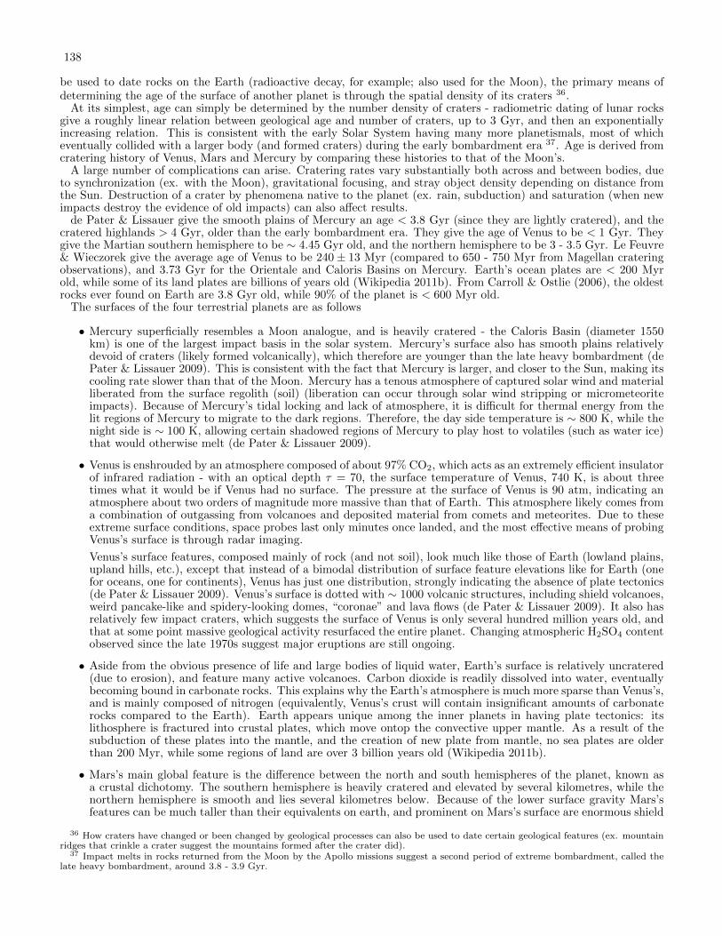
138

be used to date rocks on the Earth (radioactive decay, for example; also used for the Moon), the primary means ofdetermining the age of the surface of another planet is through the spatial density of its craters 36.

At its simplest, age can simply be determined by the number density of craters - radiometric dating of lunar rocksgive a roughly linear relation between geological age and number of craters, up to 3 Gyr, and then an exponentiallyincreasing relation. This is consistent with the early Solar System having many more planetismals, most of whicheventually collided with a larger body (and formed craters) during the early bombardment era 37. Age is derived fromcratering history of Venus, Mars and Mercury by comparing these histories to that of the Moon’s.

A large number of complications can arise. Cratering rates vary substantially both across and between bodies, dueto synchronization (ex. with the Moon), gravitational focusing, and stray object density depending on distance fromthe Sun. Destruction of a crater by phenomena native to the planet (ex. rain, subduction) and saturation (when newimpacts destroy the evidence of old impacts) can also affect results.

de Pater & Lissauer give the smooth plains of Mercury an age < 3.8 Gyr (since they are lightly cratered), and thecratered highlands > 4 Gyr, older than the early bombardment era. They give the age of Venus to be < 1 Gyr. Theygive the Martian southern hemisphere to be ∼ 4.45 Gyr old, and the northern hemisphere to be 3 - 3.5 Gyr. Le Feuvre& Wieczorek give the average age of Venus to be 240± 13 Myr (compared to 650 - 750 Myr from Magellan crateringobservations), and 3.73 Gyr for the Orientale and Caloris Basins on Mercury. Earth’s ocean plates are < 200 Myrold, while some of its land plates are billions of years old (Wikipedia 2011b). From Carroll & Ostlie (2006), the oldestrocks ever found on Earth are 3.8 Gyr old, while 90% of the planet is < 600 Myr old.

The surfaces of the four terrestrial planets are as follows

• Mercury superficially resembles a Moon analogue, and is heavily cratered - the Caloris Basin (diameter 1550km) is one of the largest impact basis in the solar system. Mercury’s surface also has smooth plains relativelydevoid of craters (likely formed volcanically), which therefore are younger than the late heavy bombardment (dePater & Lissauer 2009). This is consistent with the fact that Mercury is larger, and closer to the Sun, making itscooling rate slower than that of the Moon. Mercury has a tenous atmosphere of captured solar wind and materialliberated from the surface regolith (soil) (liberation can occur through solar wind stripping or micrometeoriteimpacts). Because of Mercury’s tidal locking and lack of atmosphere, it is difficult for thermal energy from thelit regions of Mercury to migrate to the dark regions. Therefore, the day side temperature is ∼ 800 K, while thenight side is ∼ 100 K, allowing certain shadowed regions of Mercury to play host to volatiles (such as water ice)that would otherwise melt (de Pater & Lissauer 2009).

• Venus is enshrouded by an atmosphere composed of about 97% CO2, which acts as an extremely efficient insulatorof infrared radiation - with an optical depth τ = 70, the surface temperature of Venus, 740 K, is about threetimes what it would be if Venus had no surface. The pressure at the surface of Venus is 90 atm, indicating anatmosphere about two orders of magnitude more massive than that of Earth. This atmosphere likely comes froma combination of outgassing from volcanoes and deposited material from comets and meteorites. Due to theseextreme surface conditions, space probes last only minutes once landed, and the most effective means of probingVenus’s surface is through radar imaging.

Venus’s surface features, composed mainly of rock (and not soil), look much like those of Earth (lowland plains,upland hills, etc.), except that instead of a bimodal distribution of surface feature elevations like for Earth (onefor oceans, one for continents), Venus has just one distribution, strongly indicating the absence of plate tectonics(de Pater & Lissauer 2009). Venus’s surface is dotted with ∼ 1000 volcanic structures, including shield volcanoes,weird pancake-like and spidery-looking domes, “coronae” and lava flows (de Pater & Lissauer 2009). It also hasrelatively few impact craters, which suggests the surface of Venus is only several hundred million years old, andthat at some point massive geological activity resurfaced the entire planet. Changing atmospheric H2SO4 contentobserved since the late 1970s suggest major eruptions are still ongoing.

• Aside from the obvious presence of life and large bodies of liquid water, Earth’s surface is relatively uncratered(due to erosion), and feature many active volcanoes. Carbon dioxide is readily dissolved into water, eventuallybecoming bound in carbonate rocks. This explains why the Earth’s atmosphere is much more sparse than Venus’s,and is mainly composed of nitrogen (equivalently, Venus’s crust will contain insignificant amounts of carbonaterocks compared to the Earth). Earth appears unique among the inner planets in having plate tectonics: itslithosphere is fractured into crustal plates, which move ontop the convective upper mantle. As a result of thesubduction of these plates into the mantle, and the creation of new plate from mantle, no sea plates are olderthan 200 Myr, while some regions of land are over 3 billion years old (Wikipedia 2011b).

• Mars’s main global feature is the difference between the north and south hemispheres of the planet, known asa crustal dichotomy. The southern hemisphere is heavily cratered and elevated by several kilometres, while thenorthern hemisphere is smooth and lies several kilometres below. Because of the lower surface gravity Mars’sfeatures can be much taller than their equivalents on earth, and prominent on Mars’s surface are enormous shield

36 How craters have changed or been changed by geological processes can also be used to date certain geological features (ex. mountainridges that crinkle a crater suggest the mountains formed after the crater did).

37 Impact melts in rocks returned from the Moon by the Apollo missions suggest a second period of extreme bombardment, called thelate heavy bombardment, around 3.8 - 3.9 Gyr.

139

volcanoes in the Tharsis region, and a large canyon system, Valles Marineris, that formed along with the Tharsisregion volcanoes. These volcanoes were active until ∼ 2 Myr ago. It is most likely that the entire surface ofMars is more than 4 Gyr old, and the northern plains were resurfaced later. Two hypotheses for why the crustaldichotomy exists are large-scale mantle convection and a giant impact.

Mars’ surface and atmosphere are both quite red, indicative of high concentrations of FeO2. This is perhapsbecause the planet cooled faster than Earth, preventing Mars from undergoing the same degree of gravitationalseparation.

At 6 mbar and a temperature around 130 - 300 K, all water is either solid or vapour (indeed, a thin layer offrost forms on Mars’s surface each night, to sublimate away at dawn). CO2 in the atmosphere will also condenseout in the winter, forming the dry ice polar caps (which, therefore, grow and recede every Martian year). Marsalso has plenty of features that look like they were carved out by water; whether or not it still flows today iscontroversial. Regardless, Mars is very likely to have had large amounts of water in the past, and significantreservoirs of it exist today either frozen in the ice caps, or in the Martian permafrost in upper and mid-latitudes.

This section was from de Pater & Lissauer (2009) Ch 5.5.4.

4.9.1. Compare the interiors of the inner planets.

All four inner planets (Fig. 86) have stratified interiors (i.e. an iron core surrounded by a mantle and crust oflighter material) due to gravitational differentiation of heavy and light materials. Among the four, Mercury has thelargest iron core, suggesting that much of the outer material was stripped away by a giant impact with an object afifth its mass early in its history. Mars, being close to Jupiter, was sapped of planetismals due to the giant planet’sgravitational cross-section, and is therefore smaller than the other terrestrial planets. This is insufficient to explainMars’ lack of iron, though (it has a lower density than Earth and Venus); the reason for this dearth of iron is not yetunderstood.

Fig. 86.— Comparison of the interiors of the inner planets and the Moon. From Bennett et al. (2007), their Fig 7.2.

4.9.2. Why are there tectonic plates on Earth, but not other planets?

The information in this section comes from Valencia et al. (2007).The appearance of plate tectonics on terrestrial planets is related to planetary mass. In order for plates to move,

convective stresses in the mantle have to be large enough to overcome lithospheric resistance to deformation, and theplate has to reach negative buoyancy to drive subduction. As planetary mass increases, the shear stress available toovercome resistance to plate motion increases while the plate thickness decreases, thereby enhancing plate weakness.A thinner crust also allows it to be negatively buoyant.

Earth-mass objects are at the limit at which plate tectonics will naturally occur, at which point other processesbecome important. On Venus, high surface temperatures may mean a layer of Venus’s crust is highly deformable,reducing the chances for Venus’s crust to fracture. On Earth, material permeated with water tends to be less tolerantof stresses. Objects with less than an Earth mass have crusts that can withstand mantle convection.

4.9.3. Why has Mars lost its atmosphere while Venus has not?

Atmospheres are replenished by outgassing (volcanic eruptions), evaporation/sublimation of solids and surface ejec-tion of particles from cosmic ray and micrometeorite impacts (Bennett et al. 2007). Atmospheres are depeted bycondensation, chemical reactions, solar wind stripping and thermal escape (where a small part of the tail of theatmosphere’s Maxwell-Boltzmann distribution has the escape velocity) (Bennett et al. 2007).

Mars once was warm enough to have a convecting outer core, which, coupled with its rotation, produced a substantialmagnetic field to ward off solar wind stripping. As Mars cooled at a much more substantial rate than Earth or Venus

140

(because it is smaller), the magnetosphere weakened, and outgassing was reduced. The atmosphere was therefore notbeing replenished, and what gases it did have were eventually stripped away by the solar wind, or, in the case of water,dissociated by UV radiation and then ejected via thermal escape. Some gas also condensed onto the surface due tothe declining greenhouse effect from a thinning atmosphere.

Due to its slow rotation, Venus also does not have a strong magnetic field, and its upper atmosphere is bombardedby solar wind particles. It has, however, higher surface gravity than Mars, and its interior is still warm due to itslarger mass. As a result, outgassing is still significant, and loss mechanisms from solar radiation are dampened (sinceescape velocity is higher). Because of high temperatures from the runaway greehouse effect, the atmosphere stays ingas form.

4.9.4. Why does Venus have a much thicker atmosphere than Earth?

Naively one would expect Venus and Earth to have the same atmospheres (with Venus being somewhat hotter). Theproximity of Venus to the Sun, however, gave it a higher surface temperature, resulting in more water evaporationthan on Earth (Carroll & Ostlie 2006). This lead to a runaway greenhouse effect whereby all liquid water on Venus’surface vapourized. Because water is needed for CO2 sequestration into carbonate rocks, outgassed CO2 was neverreprocessed, and remained in the atmosphere (Bennett et al. 2007). Earth has 105 times more CO2 dissolved incarbonate rock than in the atmosphere, explain why our atmosphere is much thinner than that of Venus (Bennettet al. 2007). The water, lighter than CO2, floated to the top of the atmosphere, where it was photodissociated by solarUV radiation. The hydrogen (being lighter but having the same temperature as the rest of the atmosphere) was thenpeeled away through thermal escape, while the oxygen sequestered into rock (Bennett et al. 2007).

4.10. Question 10

QUESTION: What is the Eddington Luminosity? Give examples where it is important.

A system that emits copious amounts of radiation will naturally feel a radiation pressure - each electron will seethe photons from its neighbours. Suppose the electron sees a flux S (we reserve F for force). Since each photon ofenergy E imparts momentum p = E/c, the pressure from this flux is S/c. If we assume all atoms are ionized, then theelectron cross-section can be approximated as the Thomson scattering cross-section σT = 6.65×10−25 cm2. This givesus F = σT

c S. If we now assume the system is spherically symmetric and optically thick and we are concerned mostlywith the outer layers (photosphere if the system is optically thick) blowing off, we approximate S with a blackbody,and:

Fph =σT

c

L

4πr2, (159)

where r is the radius of the photosphere. Equating this to the force of gravity Fg = GMmpnne/r2 (nuclei are

electromagnetically coupled to electrons and tend to flow with them even if the system is ionized), where nne is thenumber of nucleons per electron (1 for hydrogen, 2 for carbon and oxygen):

LEdd =4nneπGMmpc

σT(160)

An equivalent method (Carroll & Ostlie 2006, pg. 341) of looking at this through bulk properties, rather than the

force balance on a single electron. We recall dPrad

dr = − κρc Frad from Sec. 4.3. We again equate Frad = L/4πr2. If theradiation pressure provides the exact pressure gradient to conteract gravity, then

− κρc

L

4πr2= −GMρ

r2(161)

From this we can derive

LEdd =4πGc

κM (162)

Note that κ = σT /nnemp, which simply indicates opacity is a cross-section per unit mass of material.The Eddington Luminosity is an important feature of many astrophysical systems, since a process that produces a

larger luminosity must then drive an outflow. AGB-tip stars, for example, may exceed the Eddington Luminosity anddrive a superwind. Steady-state accretion onto objects (see below) is also limited by the Eddington Luminosity - iftoo much mass is dumped onto an object at once, the increase in the object’s luminosity can drive an outflow, buoyingthe infalling material and driving accretion rates down to the Eddington accretion rate.

141

4.10.1. What is the Eddington accretion rate?

A related value is the Eddington accretion rate. Suppose accretion is approximated as spherical, and gravitationalpotential energy is turned into radiation with efficiency ε. The mass accretion rate corresponding to LEdd is then:

mEdd =4nneπGMmpc

σT ε∆φ. (163)

∆φ is the amount of potential energy lost per unit mass accreted. In a stationary system (i.e. looks the same forall time) all the mass is moving closer to the accretor, and the net energy loss is equal to mGM/R, where R is theradius of the accretor (visualize a long chain of particles moving radially toward the accretor to convince yourself ofthis), making ∆φ = GM/R. For disk accretion ε ∼ 0.1.

4.10.2. Under what conditions does the Eddington luminosity not apply?

Many astrophysical systems (in particular disk accretion) do not radiate isotropically. Moreover, this entire derivationimplicitly assumes the system is stationary (since it is at equilibrium); astrophysical systems can easily exceed LEdd

temporarily, such as SN, where the photons drive a radiation pressure-dominated outflow.

4.11. Question 11

QUESTION: State the central temperature of the Sun.

The central temperature of the Sun is 1.57 × 107 K. The central pressure is 2.342 × 1016 N/m2, and the centraldensity is 1.527 × 105 kg/m3 (Carroll & Ostlie 2006, pg. 351). (The hydrogen content is only 0.34, and the heliumcontent is 0.64, due to 5 Gyr of nuclear processing.)

We can perform a very simple estimate of the central temperature, pressure and density of the Sun using thehydrostatic equilibrium equation and the ideal gas law. Assuming dP/dm → ∆P/M , r → R/2, m → M/2 (andPs = 0) we obtain

Pc =2GM2

πR4(164)

The average density of the star is ρ = 3M4πR3 . The ideal gas law at the centre of the star is Pc = ρc

µmHkBTc. Combining

these things together, we obtain:

Tc =8µmHGM

3kBR

ρ

ρc(165)

Assuming that ρc ≈ ρ, we obtain Tc = 3× 107 K, Pc = 7× 1014 Pa and ρc = 1.4× 103 kg/m3.

4.11.1. What assumptions have you made, and how good are they?

We assume that the average density is of the same order of magnitude as the central density, but this is a severeunderestimate - more detailed models suggest by a factor of 102. As it turns out we are also underestimating the centralpressure, which is much higher; this is because pressure is not a linear function inside a star. Our mean molecularweight was assumed to be 0.5; in fact it should be closer to 1, since the Sun’s core is made of more He than H. Weassume the Sun is not rotating - it in fact is, but at a rate about 0.5% its breakup velocity (a correction, known asthe Chandrasekhar approximation, can be made by adding 2

3ρΩ2r2 to the hydrostatic equilibrium equation). The Sunhas an outer convection zone, which ostensibly changes the central temperature, but since luminosity is governed bythe much longer radiative diffusion time (through the radiative zone), and, by mass, convection only makes up a fewpercent of the Sun. Indeed, much better estimates of central values can be obtained just by assuming an appropriatepolytrope and integrating.

Fig. 87 shows the temperature, pressure, density, mass, luminosity and inverse gradient structure of the Sun, ascomputed by modern models.

4.11.2. Why are the centres of stars so hot?

Because they are massive gravitating bodies, by the equation of hydrostatic balance dPdr = −Gmρr2 there needs to be

a pressure gradient within the star. This results in an extremely high central pressure, and since pressure in a mainsequence star is provided by non-degenerate gas pressure, and per the ideal gas law, P = ρ

µmHkBT , a high thermal

energy density fρcV T is needed. Stars radiate as blackbodies, and so over time the thermal energy needed to holdthe star up is lost. To replenish it, a star’s central temperature must be high enough to light nuclear fusion, whichgenerates enough energy to maintain a high thermal energy density at the star’s core. This, in essense, is why thecentre of stars are so hot.

142

Fig. 87.— Various properties of the Sun as a function of normalized radius. dLr/dr may seem strange at first, but recall this is a radialderivative of something that depends on volume. Also note that the gradient plotted is d lnP/d lnT , rather than the more common reverse.From Carroll & Ostlie (2006), their Figs 11.4 - 11.7.

4.12. Question 12

QUESTION: Which have higher central pressure, high-mass or low-mass main-sequence stars?Roughly, what is their mass-radius relation? Derive this.

Let us combine Array 128 with the ideal gas law, which says P ∝ ρT ∝ MR3T . Combining P ∝ M2

R4 with P ∝ ρT ∝MR3T nets us

T ∝ M

R. (166)

Combining this with T 4 ∝ MR4L gives us

L ∝M3 (167)

Note that the empirical relation is L ∝ M3.2, reasonably close to this value (Kippenhahn & Weigert 1994, pg. 209).Now, recall from 4.21 that the p-p chain has energy generation per unit mass ε ∝ T 4

c and the CNO cycle has energygeneration per unit mass ε ∝ T 20

c , in the range of 107 K, which is the approximate central temperature of our Sun.L ∝Mε ∝M3 38, which gives us ε ∝M2. For both the p-p chain (Tc ∝M1/2) and CNO cycle (Tc ∝M1/10), mass isa very shallow function of temperature.

The main sequence contains stars from the hydrogen burning limit (0.08 M) to around 100 M, and switchesfrom being p-p chain to CNO cycle dominated at around 1 M (Kippenhahn & Weigert 1994, pg. 212). Centraltemperature, then, changes by less than one order of magnitude, according to our scaling relations. We assume it is aconstant.

38 L ∝Mε suggests that the amount of material currently undergoing fusion is linearly proportional to the total mass of the system.

143

At this point, there is a bit of an ambiguity: does temperature in Eqn. 166 refer to central or surface temperature?Marten’s solution is to assume that Tc ∝ M

R , from which the mass-radius relation follows immediately:

M ∝ R, (168)

and from Pc ∝ MR3Tc we obtain

Pc ∝M−2. (169)

(The same result is obtained if we use P ∝ M2

R4 .)Alternatively, we can assume Eqn. 166 refers to exterior temperature T . This, however, is wrong, since luminosity

is related to the central temperature, while the photosphere temperature has to do with the “response” of the star tohaving a particular central temperature, density and fusion rate.

We obtain that radius either scales linearly or quite shallowly with mass, and pressure scales with the inverse ofmass (more massive stars have less central pressure). The latter point should not be surprising - 100 M stars likeEta Carinae can barely hold themselves together, while stars like the Sun have no such problem.

More advanced modelling techniques net the general formula

R ∝M1−n3−n , (170)

noting that γ = CPCV

= 1 + 1n . While generally useful (ex. for a non-relativistic WD), this expression fails for the

Sun, which can be approximated by an n = 3 polytrope. (In the Sun, if we assume κl/m is a constant (not a badassumption), then radiation pressure (Prad ∝ T 4) divided by gas pressure will also be a constant. As a result, P ∝ T 1/4.Combining this with the ideal gas equation gives us P ∝ ρ4/3, an n = 3 polytrope.)

Assuming a stationary, radiation-dominated star with a uniform composition, and power-law representations for thedensity, power generated by fusion and opacity (Kippenhahn & Weigert (1994), Eqn. 20.9), we find that R/R′ =(M/M ′)z1 , where primes indicate a different star, and z1 ranges from 0.4 to 0.8, depending on whether the p-p chain

or CNO cycle are used. We also find P/P ′ = M2R′4

M ′2R4 (since the solution is a homology it does not matter if we are

describing central or average pressure), so very roughly P ∝M−0.4, again giving us that pressure should decrease withmass. Homology relations also give us Tc ∝ M0.4 while ρc ∝ M−0.8 (the last can be derived from the ideal gas lawand the Tc and P scalings).

Detailed numerical calculations of main sequence models allow us to obtain R ∝M0.68 and L ∝M3.2; combining thiswith L ∝ R2T 4, where T is surface temperature, we can obtain the slope of the main sequence on a colour-magnitudediagram:

L ∝ T 7 (171)

4.12.1. Why do we use the radiative diffusion equation rather than a convection term?

The photon diffusion rate, which ultimately sets the luminosity (thermal energy divided by the diffusion timescalegives the luminosity of the star), is determined by the radiative zone(s) of the star. Even fully convective stars will haveradiative zones in their very outermost layers, and because convective energy transport is so efficient, the timescalefor photon escape from the star is determined by this thin radiative zone. If we also assume that these thin radiativeenvelopes scale in the same manner as their thicker counterparts, the scaling relation used in the calculation above isstill valid.

4.12.2. Where does this approximation fail?

We have assumed above that the central temperature of the star is roughly constant throughout the main sequencedue to the high temperature dependence of nuclear fusion. The homology relation (Tc ∝ M0.4, ρc ∝ M−0.8) isconsistent with this. Detailed modelling, however, show that at around 1 M the density stays roughly constant whiletemperature changes half an order of magnitude. This is related to the fact that at about 1 M the star is almostcompletely radiative (Kippenhahn & Weigert, Fig. 22.7), while in the flat regions of the curve above and below, thestar is convective to a significant degree. This region is also host to two other major changes (THOUGH IT’S NOTOBVIOUS IF THEY ARE A CAUSE OR EFFECT OF THE CONSTANT DENSITY REGIME): at the upper tipof the constant density regime, temperatures are high enough for the CNO cycle to begin dominating the pp chain asthe star’s source of energy, and degeneracy effects become important for stars below 0.5 M.

4.12.3. What about extreme masses on the main sequence?

Attempts at stellar modelling for very low masses is mired by having to treat extensive convection, and the opacityof complex molecules which form in cool stellar atmospheres. Moreover, the time for the star to reach equilibriumburning can be very long.

For very massive stars, the adiabatic gradient ∇ad → 1/4, which is quite shallow, and therefore the star is largelyconvective. The adiabatic structure requires constant specific entropy s across the star. Taking the specific energy

144

Fig. 88.— A ρ − T diagram of central temperature and density for the main sequence. Different masses are labelled above the mainsequence. Labels below the main sequence indicate the relative contribution of radiation to the pressure. The p-p/CNO horizontal lineindicates which nuclear process should dominate. Dashed lines indicate lines of constant degeneracy. Note the two flat regions (qualtiativelysimilar to what is obtained by homology arguments) and the steep region around 1 M. How central pressure behaves can be inferred fromthis trend and the ideal gas law. From Kippenhahn & Weigert (1994), their Fig. 22.5.

density u = aT 4/ρ and pressure P = aT 4/3, and using the first law of thermodynamics (ds = 1T

(du− P

ρ2 dρ)

) we find

s = 4aT 3

3ρ , which nets us ρ ∝ T 3. Since P ∝ T 4, we obtain an n = 3 polytrope for a radiation-dominated star.

4.12.4. What is the scaling relation when the pressure support of the star itself is radiation-dominated?

For stars near the Eddington Luminosity, P ∝ T 4 (from Prad = 13aT

4). Combining this with P ∝M2/R4, we obtain

T ∝M1/2/R. Then combining this with T 4 ∝ MR4L gives us

L ∝M (172)

We continue to assume Tc is approximately constant, for the same reasons as listed above. This immediately gives us

P = constant (173)

and (from T ∝M1/2/R)

M ∝ R2 (174)

4.13. Question 13

QUESTION: Derive the scaling of luminosity with mass for a (mostly) radiative star. Do you needto know the source of energy for the star to derive this scaling?

We have, to good order, already completed this question in the last question, Sec. 4.12. Combining P ∝ M2

R4 with

P ∝ ρT ∝ MR3T nets us T ∝ M

R . Combining this with T 4 ∝ MR4L gives us L ∝M3. We do not need to know the source

of energy for the star (we do need to know it to determine the mass-radius relation); this is because the luminosity isset not by the rate of nuclear fusion or gravitational contraction, but by the rate at which photons can diffuse out ofthe star. This sets an energy loss rate that the star has to compensate with nuclear reactions.

When radiation pressure begins to dominate, L ∝ M , but by that point the star has become almost entirelyconvective.

4.13.1. Does more detailed modelling give better results?

This derivation comes from Hansen et al. (2004).

145

TABLE 4Power-law Indices

Energy Generation Mode λ ν Opacity Mode n s Pressure Mode χρ χTpp-chain 1 4 Thomson Scattering 0 0 Ideal Gas 1 1

CNO cycle 1 20 Kramers’ Law 1 3.5 Radiation 0 4Triple-α Process 2 40

We may once again derive scaling relations from Array 127 (though we keep opacity as a variable in the radiativetransfer equation). Now, however, we also generate power laws (see Table 4) for energy generation, opacity and pressure(equation of state): ε ∝ ρλT ν , κ ∝ ρnT−s, and P ∝ ρχρTχT . We can then write total logarithmic differentials for thehydrostatic equilibrium equation and the various power laws; i.e. d ln ε = λd ln ρ+ νd lnT . Lastly, we assume that R,ρ, T and L all have power law scaling relations with mass M . If we then write the scaling relations for ∂m

∂r = 4πr2ρ,∂P∂r = −Gmρr2 , ∂l

∂r = 4πr2ρεnuc and l = − 64π2acT 3r4

3κ∂T∂m , and insert the power laws in, we obtain the matrix equation

1.74 in Hansen et al.. The result can be found on pg. 27 of Hansen et al.. If convection is wholly used instead ofradiation as the means of energy transport, the fact that T ∝ ργ−1 replaces the radiative diffusion equation.

The results: for electron scattering opacity, CNO cycle fusion and the ideal gas law (all of which are representativeof more massive main sequence stars), R ∝M0.78 and L ∝M3. For pp chain, Kramers opacity, and the ideal gas lawalong with radiation, L ∝ M5.5, but this is not empirically reproduced. Using convection rather than radiation givesL ∝ M8.3, which is even more untenable. Evidently, something (perhaps increasing degeneracy pressure in the core,or a better treatment of convection) must be added.

Detailed modelling and empirical results can be found in Fig. 89. Over the entire range plotted, M ∝ L3.2, thoughthe exponent is highest near 1 M, at 3.88.

Fig. 89.— The mass-luminosity relationship for stars on the main sequence. The solid line gives the theoretical mass-luminosity relation-ship, while the points give observed masses derived from detatched (points) and visual (triangles) binary systems. The decreasing slope athigher masses is due to increasing radiation pressure. From Kippenhahn & Weigert (1994), their Fig 22.3.

4.14. Question 14

QUESTION: What source of pressure prevents gravitational collapse in a normal star, a white dwarf,and a neutron star? Why, physically, is there a maximum mass for the latter two? And why can wecalculate this easily for a white dwarf, but not for a neutron star?

The source of pressure preventing gravitational collapse in a normal star is gas pressure, as given by the ideal gaslaw, P = ρ

µmHkBT . The source of pressure for a white dwarf is electron degeneracy pressure, and the source of pressure

for a neutron star is neutron degeneracy pressure. Degeneracy pressure is covered in Sec. 5.12.Degeneracy pressure is physically generated by forcing electrons into increased momentum states so as to satisfy the

146

Pauli exclusion principle - the quantization of phase space requires that electrons sharing the “same” position musthave different momenta. As such, an increased compression generates a higher distribution of momentum states (i.e.the top of the Fermi sea is higher, i.e. EF is larger). Eventually, EF becomes infinite, but even then there are still alarge percentage of particles at low energies, providing little momenta, and so the maximum pressure degeneracy canprovide is finite. If the stellar structure requires a higher pressure, which would be the case past a critical mass, thencollapse sets in. The critical mass is known as the Chandrasekhar Mass, Mch, in a WD.Mch is easy to calculate for a WD (an estimate is below). If neutrons behaved like electrons, the equivalent mass for

neutron stars would also be easy to calculate, except that the radius of a neutron star is on order Rs, the Schwarzschildradius, and therefore a self-consistent general relativistic solution would be needed (Townsend 1997). Materials atneutron star densities, however, are poorly understood, as a complete theoretical description of the behaviour of a seaof free neutrons interacting via the strong nuclear force in the presence of electrons and protons does not yet exist,and there is little experimental data on the matter (Carroll & Ostlie 2006, pg. 581). Moreover, more massive baryonresonances, quark “bags”, and bose condensates of mesons might also exist at such densities (Camenzind 2007).

4.14.1. Estimate the Chandrasekhar Mass for a WD. Estimate the equivalent for an NS.

The momentum state density (i.e. number of states from p to p+dp in a volume dV ) of a fermionic gas is f(p) = 8πp2

h3 ,and in a degenerate gas the occupation number for all states less than momentum pF is 1 (and the occupation numberfor all states above is zero). The integral of f(p) from 0 to pF is equal to the number density of fermions. As a result,n = 8π

3h3 p3F , from which we can (through EF = pF /2m for non-relativistic and EF = pF c for relativistic) obtain EF ,

which is

EF =~2

2me(3π2n)2/3 (175)

for a non-relativistic gas and

EF = (3π2n)1/3~c (176)

for a relativistig gas. We then can perform a similar calculation in both cases as we did in Sec. 3.13.2. UsingξEi + Eg = 4πR3Pext, in the non-relativistic case, we have

−fgGM2

R+ fF

~2

2meµ5/3m5/3p

(3π2)2/3M5/3

R2= 4πR3Pext. (177)

In this case for R→ 0, Pext →∞, meaning the system is stable against completely collapse. (There is a turning pointin Pext(R), past which the object will collapse to the R of the turning point, but (again recalling Sec. 3.13.2) Pext = 0is inside this turning point.) Assuming Pext = 0 gives us an R ∝M−1/3 relationship.

In the relativistic case,

−fgGM2

R+ fFR~c(3π2)1/3 (M/µmp)

4/3

R= 4πR3Pext. (178)

This system is critically stable, and there is only one mass which corresponds to Pext = 0. Solving for this, we obtain:

Mch = (3π2)1/2

(fFRfg

)3/2(~cG

)3/2

(µmp)−2 (179)

fFR/fg is of order unity, and if we ignore it, we obtain 2.5 M. Due to the M2 dependence of gravitational potential

energy vs. the M4/3 dependence of Fermi energy, M > Mch stars always have negative external pressures, makingthem unstable to collapse, while M < Mch stars will expand until becoming less relativistic. We can estimate Rch bytaking the mass-radius relation for non-relativistic WD, and plugging Mch in.

Eqn. 179 is independent of electron mass, and so applies equally well to neutron star, except for neutron stars µ ≈ 1- the NS equivalent to the Chandrasekhar mass is therefore about a factor of four more massive. This turns out notto be the case for two reasons: general relativity increases the effective gravitational potential energy of the NS, andthe neutron star equation of state is much more complicated than the white dwarf equation of state.

Detailed calculations give 1.4 M for WDs, and 2.2 M for NSs (Carroll & Ostlie 2006, pg. 583).

4.14.2. Why is proton degeneracy unimportant in a WD?

While Coulombic corrections between proton-electron pairs do affect the WD equation of state, to first order protonsdo not matter in a WD except as a source of gravity. This is because degeneracy pressure is inversely proportionalto mass. Since electrons and protons have the same density at any given region in the neutron star (this is mediatedby gravity), proton degeneracy pressure becomes unimportant. Proton degeneracy pressure can become important atneutron star densities, but by this point the star is unstable to electron capture onto protons.

147

4.14.3. What is the structure of a neutron star?

This information is from (Camenzind 2007, pg. 188) and (Carroll & Ostlie 2006, pg. 581 - 582)From the outside in, a neutron star is composed of

• The cm-thick atmosphere.

• The outer crust, essentially relativistic electron degeneracy material.

• The inner crust, which extends from 4 × 1014 kg/m3 (when free neutrons begin to appear) to 2 × 1017 kg/m3

(when nuclei dissolve), which contains free neutrons, relativistic electrons and neutron-rich nuclei. The materialis superconducting. Neutron degeneracy dominates electron degeneracy past 4× 1015 kg/m3.

• The core, composed of a superconducting zero-viscosity fluid of free neutrons, protons, electrons and a possibleassortment of hyperons (more massive baryon resonances), quarks and mesons.

See Fig. 90.

Fig. 90.— A schematic of the interior of a neutron star. From Camenzind (2007), their Fig 6.1.

4.14.4. How can rotational support change the maximum mass?

Since rotational energy can help support a star, a fast-spinning WD or NS could theoretically exceed their hydrostatic(non-rotating) mass limits.

A rigidly rotating WD can have a mass up to 1.48 M, but a differentially rotating WD (with an artificiallyconstructed rotation profile) can achieve masses in excess of 4 M (Yoon & Langer 2004). WDs this massive cannotbe created by canonical stellar evolution, but they could possibly be spun up while accreting. The upper limit to adifferentially rotating WD’s mass, ∼ 2 M, is given by the maximum amount of material it could acquire by massaccretion from a companion (Yoon & Langer 2004).

2.9 M NSs are possible with significant rotational support (Carroll & Ostlie 2006, pg. 583).

4.14.5. Could you heat a WD or NS to provide thermal support?

Of course! Heat a WD enough, and in such a way as to not ignite nuclear burning, and you would have a hot cloudof H, He, C and O (and possibly Ne). Heat an NS enough, and the additional thermal pressure support will lift theNS degeneracy, and you would possibly get a cloud of hot deuterium.

148

4.15. Question 15

QUESTION: Sketch the SED of an O, A, G, M, and T star. Give defining spectral characteristics,and describe physically.

Fig. 91.— Representative spectra of main sequence, with prominent line features labelled. The spectra have been normalized at a commonwavelength, and stacked on top of each other for the sake of presentation. From Gray & Corbally (2009), their Fig 2.1.

The information for this question comes from Carroll & Ostlie (2006), Ch. 8.1, and Gray & Corbally (2009), Ch. 2.Figs. 91, 92 and 93 show the spectrum of main sequence stars from O to M from 1100 Ato 2 µm. Most prominent in

all early-type (more massive than the Sun) spectra are the Balmer lines (Hα, 6562 A; Hβ, 4861 A, Hγ, 4340 Aand Hδ,410.2 A; ionization from the first excited state occurs past 3651 A, the location of the “Balmer jump”), which increasein intensity from O to A2, and then decrease for later types, ceasing to be prominent by K type. He I follows a similarpattern, peaking in B2. He II lines are already decreasing for O stars, indicating their peak is in a range not normallyreached by stars. Ca II lines (the strongest being the H and K lines at 3968 and 3933 A) become stronger until they

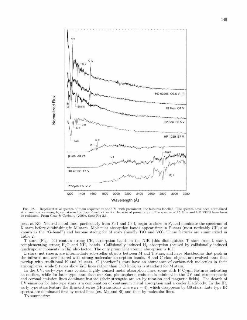
149

Fig. 92.— Representative spectra of main sequence in the UV, with prominent line features labelled. The spectra have been normalizedat a common wavelength, and stacked on top of each other for the sake of presentation. The spectra of 15 Mon and HD 93205 have beende-reddened. From Gray & Corbally (2009), their Fig 2.6.

peak at K0. Neutral metal lines, particularly from Fe I and Cr I, begin to show in F, and dominate the spectrum ofK stars before diminishing in M stars. Molecular absorption bands appear first in F stars (most noticably CH, alsoknown as the “G-band”) and become strong for M stars (mostly TiO and VO). These features are summarized inTable 2.

T stars (Fig. 94) contain strong CH4 absorption bands in the NIR (this distinguishes T stars from L stars),complementing strong H2O and NH3 bands. Collisionally induced H2 absorption (caused by collisionally inducedquadrupolar moments in H2) also factor. The only prominent atomic absorption is K I.

L stars, not shown, are intermediate sub-stellar objects between M and T stars, and have blackbodies that peak inthe infrared and are littered with strong molecular absorption bands. S and C class objects are evolved stars thatoverlap with traditional K and M stars. C (“carbon”) stars have an abundance of carbon-rich molecules in theiratmospheres, while S types show ZrO lines rather than TiO lines, as is standard for M stars.

In the UV, early-type stars contain highly ionized metal absorption lines, some with P Cygni features indicatingan outflow, while for later type stars than our Sun, photospheric emission is minimal in the UV and chromosphericand coronal emission lines dominate instead (their strengths are set by rotation and magnetic fields). The dearth ofUV emission for late-type stars is a combination of continuum metal absorption and a cooler blackbody. In the IR,early type stars feature the Brackett series (H-transitions where nf = 4), which disappears by G0 stars. Late type IRspectra are dominated first by metal lines (ex. Mg and Si) and then by molecular lines.

To summarize:

150

Fig. 93.— Representative spectra of main sequence in the IR, with prominent line features labelled. The spectra have been normalizedat a common wavelength, and stacked on top of each other for the sake of presentation. From Gray & Corbally (2009), their Fig 2.7.

1. O stars: highly ionized metals, He II absorption, weak Balmer lines.

2. A stars: strongest Balmer lines, He I no longer visible, weak neutral metal lines and Ca II H and K.

3. G stars: strong Ca II doublet, stronger neutral metal lines, G-band.

4. M stars: spectra dominated by molecular absorption bands, especially TiO. Neutral metal absorption linesremain strong.

5. T stars: molecular absorption, mainly in CH4 and H2O.

As noted earlier, absorption lines are caused by wavelength-dependent opacity in the stellar photosphere (or, equiv-alently, scattering and absorption of a blackbody by colder, tenuous material). The amount of resonant scattering andabsorption from a certain species i, j, where i is the degree of ionization and j is the degree of excitation, is dependenton amount of such species in the stellar photosphere, Ni,j .

151

Fig. 94.— Observed spectrum of a T star from 2Mass. From Gray & Corbally (2009), Fig. number unknown.

For a system in local thermodynamic equilibrium, the Boltzmann equation gives the probability of being in state jas

pj =gj exp−Ej/kBT

Z=

gj exp−Ej/kBT∑j gj exp−Ej/kBT

(180)

where Z is the partition function and gj is the degeneracy of a particular energy state. Meanwhile, the Saha Equation,which can be derived from the grand partition function, gives

Ni+1

Ni=

2Zi+1

neZi

(2πmekBT

h2

)3/2

e−χi/kBT (181)

where i indicates the degree of ionization, χi is the ionization energy from degree i to degree i + 1. The strengthof a line is given by Ni,j/Ntotal, which is given by a combination of the Boltzmann and Saha equations. Hydrogenis the easiest to calculate, since it only has one ionization state. The strength of Balmer absorption, for example, isdetermined by

NI,2Ntotal

=g2 exp−E2/kBT

ZI

1

1 +NII/NI(182)

where NII/NI = 2ZIIneZI

(2πmekBT

h2

)3/2e−χI/kBT . Eqn. 182 contains two competing temperature dependencies:

exp−E2/kBT /ZI increases with temperature (at least, up to a certain point - atoms have infinite numbers of ex-cited states, and at infinite temperature (and artificially suppressing ionization) each of these states would be equally

populated), and so does NII/NI . PlottingNI,2Ntotal

as a function of temperature, we obtain Fig. 95.In general all line strengths follow the pattern described by Fig. 95. The exception are lines in the ground state

neutral atoms, which should only increase in strength with decreasing temperature, and ions, which should alsoincrease with decreasing temperature so long as temperatures are sufficiently high for their existence (ionization is afairly sharp transition in many cases, which is what causes the sudden disappearance of these lines for sufficiently coolstars). Lyman-α (1216 A), Ca II H and K, and Ca I (4226 A) are examples of such “resonance lines”.

4.15.1. What are the primary sources of line broadening?

Lines are not delta functions, and their width can be measured either by the equivalent width W (whereFcontinuumW =

∫Fcontinuum − Fdλ) or the full-width half-maximum, which is obtained by fitting a Gaussian.

Spectral lines can be broadened by

• Natural broadening: the time-energy uncertainty principle, ∆E∆t ≈ ~, states that for a system with rapidlychanging observables (i.e. a short lifetime in a certain state), the energy cannot be entirely certain. Very roughly,

∆E of a transition is equal to ∆Ef+∆Ei, which translates to δλ = λ2

2πc

(1

∆ti+ 1

∆tf

). A more involved calculation

152

Fig. 95.— Estimate (assuming only ground and first excited state occupation for the Boltzmann equation) of the fraction of first excitedstate neutral hydrogen in a stellar atmosphere of varying temperature. ne is estimated from Pe = nekBT = 20 N/m2. The peak occurs at9900 K, corresponding to the temperature at which Balmer lines will be at their strongest. From Carroll & Ostlie (2006), their Fig. 8.9.

gives the FWHM of natural line broadening as λ2

πc1

∆t , where ∆t is the lifetime of a state before transition toanother state. Natural broadening forms a Lorentz profile.

• Doppler broadening: this occurs because the atoms are Maxwell-Boltzmann distributed, with a most probable

velocity vmp =√

2kBTm . ∆λ = 2λ

c vmp is a decent estimate. Integration over the distribution gives the FWHM as

2λc

√ln 2

(2kBTm + v2

turb

), where vturb is the most probable turbulent velocity (turbulent velocity is assumed to be

Maxwell-Boltzmann distributed). Turbulence is of importance in giant and supergiant stars. Non-Maxwellianbroadening, such as in fast-rotating, pulsating or superwind stars, also affect spectra.

• Pressure (and collisional) broadening: pressure broadening occurs when an atoms orbital structure ismodified by a large number of closely passing ions. Close encounters with ions and collisions with neutralatoms also can disturb orbitals. We can estimate the effect of line broadening by setting the ∆t in the naturalbroadening equation to ∆t = l/v = 1

nσ√

2kBT/m. Pressure/collision line broadening is therefore proportional to

both temperature and density.

The combined line profile from these effects is known as the Voigt profile. The core of a Voight profile is dominatedby Doppler broadening, while the wings by the Lorentz profile of natural and pressure broadening (this is because aLorentz profile does not decay as quickly).

4.15.2. What is the curve of growth?

The curve of growth is a plot of W as a function of Na, the abundance of a certain atom in the stellar atmosphere(Na can be thought of as a column density). In the regime where the absorption line is optically thin (i.e. at itsresonant wavelength, not all the light from the background is absorbed), W cales with Na. Once the centre of theline becomes optically thick (and absorbs all incoming radiation at the resonant wavelength), the optically thin wingscontinue to grow, and W scales like

√lnNa. If Na continues to increase, it reaches a stage at which pressure line

broadening exceeds natural line broadening, and W begins to scale like N1/2a .

4.15.3. How is a P Cygni feature produced?

A P Cygni profile consists of a blueshifted absorption line alongside a redshifted emission line (see Fig. 96), and iscaused by an outflow. The blueshifted absorption is caused by continuum absorption due to material headed toward theobserver, while the redshifted emission comes from re-radiation of absorbed photons (due to the same transition) frommaterial headed away from the observer. The rest-frame resonant emission comes from material moving perpendicularto the observer. An inverted P Cygni profile indicates accretion.

4.15.4. What are the main differences between supergiant and main sequence spectra, assuming the same spectral classification?

Absorption lines in a supergiant are generally narrower than their dwarf star counterparts, as they have tenuous,extended (but still optically thick) atmospheres and therefore low surface densities at there photospheres. A reducedelectron density also increases ionization, and therefore the Balmer lines (for example) will be suppressed at lower

153

Fig. 96.— Schematic of a P Cygni profile, annotated to describe how each component of the feature is created. From Carroll & Ostlie(2006), their Fig. 12.17.

temperatures. These features are used to determine the Morgan-Keenan (MK) luminosity class, which can then beused to determine the (approximate) luminosity of the star.

4.16. Question 16

QUESTION: What physical and orbital parameters of an extra-solar planet can be determined a).from radial velocity (Doppler) measurements alone, b). from transit observations alone, and c). fromthe combination of both Doppler and transit observations?

Most of the information here comes from Santos (2008) and Seager (2010).A planet-star system will orbit a common centre of mass. As the star orbits this centre of mass, its radial velocity

will shift sinusoidally, with an amplitude that depends both on the star’s orbital velocity v and the inclination of thesystem to us, i (where i = 0 means the system is edge-on to us). We may measure vs sin i using ∆λ

λ = vs sin i/c. While

the typical spectrograph resolution (0.1 A) is insufficient to detect vs sin i (typically ∆λ = 10−4 A) using a single line,fitting for the entire stellar spectrum can greatly increase accuracy - errors of 1 - 100 m/s are achievable.

Using the fact that Ms/Mp = vp/vs = ap/as (i.e. the CM has position 0 and does not move), v = 2πa/P andKepler’s Third Law, we are able to find that Ks = vs sin i has the form

Ks = 2πG

(Ms

P

)1/3q

(1 + q)2/3

sin i√1− e2

. (183)

where q = Mp/Ms. Generally, the “mass function” f(M) =PK3

s

2πG =Mp sin3 i(1+q)2 is reported. 1 + q ≈ 1 for planets, and

all other quantities except for q and sin i can be measured: P is obtained from timing the period of radial oscillatorymotion, and ap can be found by noting that Msas sin i = Mpap sin i and noting we know Ms, as sin i and Mp sin i. ecan be determined by the shape of the binned velocity curve. It is not possible to obtain i, and therefore we can onlyfind a minimum mass using radial velocities (statistically, there is an 87% chance sin i > 0.5, as there is a bias againstfinding low-inclination orbits.

Transits occur when the star and planet orbit line up so that, from the perspective of an observer, the planetperiodically passes in front of its parent star (Fig. 97). Full transit probability can be estimated by p = Rs/a,indicating that a close-in planet orbiting a giant star is much more likely to be spotted via transit assuming any transitthat occurs can be detected. The dip in starlight due to a transiting planet can be estimated as

∆L

L≈(RPRS

)2

. (184)

For Jupiter transiting the Sun, a ∼ 1% drop in the Sun’s luminosity is expected. Since a large ∆L/L is easier todetect, giant planets and small stars are favoured.

A transit schematic is given in Fig. 97. As the planet moves in front of the star, there will be two periods of time(between I and II and between III and IV on the schematic) where only part of the planet is blocking any starlight;these periods are known as ingress (I - II) and egress (III - IV) (periods are denoted τing and τegr, and the two valuesare generally almost the same) (Seager 2010). These times, along with the total transit time, may be used to determinethe impact parameter (b in Fig. 97) and Rs/a, which can then be used to determine the inclination angle i (see Seager2010, pg. 60). In reality, the star is not a uniform disk, and a model of limb darkening must be used to accuratelydetermine ingress and egress times.

If secondary eclipses are visible, it is actually possible to constrain the eccentricity and angle between transit andperiastron (Seager 2010). The semi-major axis can be found if the star’s mass is known. More complex features on

154

Fig. 97.— A schematic of a transient and its ideal light curve, assuming that the star is a uniform disk and the planet uniformly absorbsall light. The four times correspond to I). when the planet first begins to transit the star, II). when the entire cross-section of the planetis within the stellar disk, III). last point in the transient when the entire planet cross-section is within the stellar disk, and IV). end oftransient. Changing the impact parameter b will change the ratio of the time period between I and II (or III and IV, which is almostidentical) and I and IV. Limb darkening is not modelled here. From Seager (2010), their Ch. 2, Fig. 2.

both the star and the planet (such as sunspots or rings) can be determined through modelling of the transit lightcurve. The mass, however, cannot be determined.

From this, we can see that if we had only radial velocity measurements, we would be able to determine the semi-majoraxis (if we knew the mass of the star), period and orbital eccentricity. The mass will only be determined up to Mp sin i.If we had only transits, we would know i, planetary radius (assuming we know the stellar radius)39, semi-major axis (ifthe parent star mass is known), eccentricity (if secondary eclipses are visible) and period. If we knew both, we wouldhave all orbital properties (semi-major axis, period, orbital eccentricity and inclination) and all planetary properties(mass, radius and average density). If no information about the star is included, planetary masses and radii would beknown only up to scaling constants for the stellar radius and mass, though we would still be able to determine periodand eccentricity (Seager 2010).

A number of curious properties can be determined without any knowledge of the parent star. So long as the period

and RS/a is known (both determined from transits), one can determine ρS +R3P

R3SρP (Seager 2010, pg 60). Since the

latter term is tiny, this provides a means of constraining stellar modes through the mean stellar density ρS . Withradial velocities and transits combined, one can determine the surface gravity of the planet using the star’s radialvelocity, the period, inclination and RP /a (derivable from RP /RS and RS/a) (Seager 2010).

Transits and radial velocities are binned in order to increase signal-to-noise. If, however, the orbit precessed, or ifthe planet has other planetary bodies exerting gravitational forces on it, then the time of the transient and the shapeof the radial velocity curve will change. Practically, transit timing has much greater sensitivity, and is often used toinfer the existence of additional, unseen planets in a stellar system (changes in orbit will also effect the shape of thetransit, which could also be used) (Seager 2010). If transits are observed at multiple wavelengths, how the shapesof the transit ingress and egress change with wavelength relates to the optical properties of the planet’s atmosphere(Seager 2010).

4.16.1. What methods are there to detect planets?

There are six methods by which exoplanet detection is made:

• Radial velocity measurements.

• Transits.

39 Technically the mass can be determined here from the mass-radius relation, but as noted in Sec. 4.2, the mass-radius relation forgiants is flat.

155

• Astrometry - measurement of the semimajor axis, as, of the orbit of a planet-hosting star, and the period P ,allows us to measure the mass of the planet via P 2 = 4π2a3/G(Mp + Ms) and as = Mpa/(Ms + Mp), if themass of the star Ms is known. In practice the entire system can be inclined to us, but ellipse fitting and radialvelocity measurements can help disentangle any degeneracies. Stellar activity may also shift the photocentre ofa star, creating false astrometric movements. A more pressing concern is the fact that the expected astrometricproper motions of stars reacting even to Hot Jupiters is of order 1 µas at best, and as of 2008 no instrumentcould definitively obtain astrometric evidence of the existence of a planet without radial velocity or transit datato reinforce the case. Note that this same procedure can be used to determine the masses of unseen stellar-masscompanions much more easily. If the companion is visible, as1 and as2 can both be measured, allowing us tosolve for Ms1 and Ms2.

• Gravitational lensing - not generally used.

• Pulsar timing - planets orbiting pulsars can shift the pulsar pulsation rate in a regular manner.

• Direct imaging - through stellar masking, faint emission/reflection from the neighbourhood of the star can bedetected. This method can be used to observe dust disks as well as find planets.

4.16.2. What are common issues when using radial velocities and transits?

Intrinsic stellar features, like non-radial pulsation, inhomogeneous convection, or starspots may be responsible forthe detection of radial-velocity variations. These hamper planet detections using radial velocities both by adding noiseto signal, and by creating false positives. Starspots, eclipsing stellar binaries, dwarves eclipsing giants, and blendedeclipsing binary systems may create false positives in transit searches. Many of these false positives can be weededout by looking for suspicious patters in the transit photometry (ex. starspots do not form secondary eclipses, and aretemporary, eclipsing stellar binary transits are dominated by ingress/egress).

4.16.3. How do Hot Jupiters form?

Gas giants need to form beyond the snow line, as water ice and other volatiles are needed to build cores of 10 Earthmasses or greater, at which point gas accretion can begin in earnest. In particular, there simply was never enoughmaterial in the vicinity of Hot Jupiters to have constructed them. The solution to this issue is planetary migration.

Type I planetary migration involves interactions between the planet and density waves in the accretion disk, which aregenerated by non-axisymmetry perturbations of the disk. Density-wave planet interactions tend to transfer angularmomentum outward and mass inward, and are proportional to mass, meaning that as planets develop the effectstrengthens. It is possible for a planet that started forming beyond the snow line to collide with the star in 107 − 108

years. Type I migration ends when the planet accretes enough (locally, since its movement through the accretiondisk brings it fresh material) to form a gap in the accretion disk. Type II migration occurs once the gap is formed -maintenance of the gap results in the planet coupling to the viscous evolution of the accretion disk (which, of course,tends toward rigid rotation), generally driving the planet closer to the star. Type II migration is general slower thanType I migration. Gravitational scattering between planets and other planets or planetismals can drive inward oroutward migration, depending on the nature of the scattering.

In our own Solar System, it is likely that Jupiter migrated about 0.5 AU inward from where it formed, while Saturn,Uranus and Neptune migrated outward. During this motion, the outer planets passed through certain resonances witheach other and with minor bodies, displacing significant numbers of objects.

4.17. Question 17

QUESTION: What spectroscopic signatures help distinguish a young (pre-main sequence) star froma main sequence star of the same spectral type?

Most of this information is from Carroll & Ostlie (2006) Ch. 12.3, and cribbed from Emberson (2012). Followupsare from the same sources.

A young stellar object (YSO) is a star that has yet to settle on the ZAMS and include both protostars and pre-mainsequence stars (the dividing line between the two is the appearance of significant amounts of outflowing material,which ends the spherical accretion phase and begins the disk accretion phase). Most of the internal evolution of thesestars, such as the switch between gravitational contraction and nuclear fusion, cannot be seen, and so instead YSOsare classified spectroscopically (see below) into Class 0, I, II and III. These classes trace out evolution over time, as bythe time a YSO reaches Class II or III (which we will denote “late-type”), bipolar outflows have cleared out much ofthe material surrounding the pre-main sequence star, and we are left with a star, disk and substantial outflow material.A schematic of this process can be found in Fig. 98

Photometric and spectroscopic signatures of late-type YSOs (i.e. the ones that have ejected much of their surroundingmaterial) include:

• Emission lines in the optical from regions of the hot disk and/or the outflow. These lines may include theBalmer series, the Ca II H and K lines, and forbidden lines [O I] and [S II], which are evidence of a very tenuous

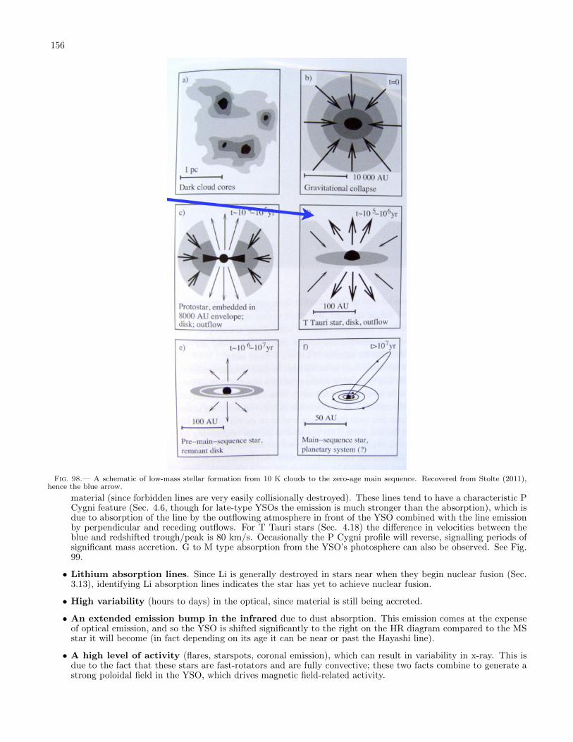
156

Fig. 98.— A schematic of low-mass stellar formation from 10 K clouds to the zero-age main sequence. Recovered from Stolte (2011),hence the blue arrow.

material (since forbidden lines are very easily collisionally destroyed). These lines tend to have a characteristic PCygni feature (Sec. 4.6, though for late-type YSOs the emission is much stronger than the absorption), which isdue to absorption of the line by the outflowing atmosphere in front of the YSO combined with the line emissionby perpendicular and receding outflows. For T Tauri stars (Sec. 4.18) the difference in velocities between theblue and redshifted trough/peak is 80 km/s. Occasionally the P Cygni profile will reverse, signalling periods ofsignificant mass accretion. G to M type absorption from the YSO’s photosphere can also be observed. See Fig.99.

• Lithium absorption lines. Since Li is generally destroyed in stars near when they begin nuclear fusion (Sec.3.13), identifying Li absorption lines indicates the star has yet to achieve nuclear fusion.

• High variability (hours to days) in the optical, since material is still being accreted.

• An extended emission bump in the infrared due to dust absorption. This emission comes at the expenseof optical emission, and so the YSO is shifted significantly to the right on the HR diagram compared to the MSstar it will become (in fact depending on its age it can be near or past the Hayashi line).

• A high level of activity (flares, starspots, coronal emission), which can result in variability in x-ray. This isdue to the fact that these stars are fast-rotators and are fully convective; these two facts combine to generate astrong poloidal field in the YSO, which drives magnetic field-related activity.

157

Fig. 99.— Optical spectra of various types of YSOs, normalized to unity at the peak of Hα emission. In the Class I and I/II sources allabsorption is due to the Earth’s atmosphere, and not intrinsic to the object. From Gray & Corbally (2009).

4.17.1. How are YSOs classified spectroscopically?

Fig. 100.— Continuum emission from different classes of YSOs. From Emberson (2012).

YSOs are intrinsically faint in the optical due to being surrounded by dust envelopes or disks. This is why their

158

classification uses the power law index

α ≡ d ln(λFλ)

d lnλ(185)

over the wavelength interval 2µm . λ . 25µm. Class 0 sources have negiligible emission shortward of 10 µm, ClassI have 0 < α < 3, Class II has −2 < α < 0 and Class III has −3α− 2, which more closely resembles ZAMS stars. SeeFig. 100.

Alternatively, we can define classes using a bolometric temperature: Class 0 has T < 70 K, Class I has 75 K < T <650 K, Class II has 650 K < T < 2880 K, and Class III has T > 2880 K.

Classes correspond to different stages of the lives of YSOs:

• Class 0 YSOs are cloud cores just beginning their collapse into YSOs.

• Class I YSOs lie in a cocoon of CSM that is assembling itself into a disk. Near the end of Class I an outflowbreaks out from the star and ejects much of the CSM.

• Class II YSOs undergo disk accretion but are still surrounded by residual material.

• Class III YSOs have moved beyond the accretion stage but have yet to move onto the ZAMS.

See Fig. 101.

Fig. 101.— Schematic of the physical nature of various YSO types. From Emberson (2012).

4.17.2. How do YSOs evolve on the HR diagram?

The rough trajectory of YSO evolution is given by the classical model of star formation (Sec. 3.13, in particular Fig.64). If accretion is slow, then the object falls down and leftward along the Hayashi track (it will deviate upward and tothe left if accretion is increased) until the luminosity decreases enough so that the interior becomes radiative (this doesnot occur for very low-mass stars, which simply “drop” along the Hayashi line until they reach their ZAMS positions).The luminosity then begins to increase once more. For an ideal gas with no nuclear generation, L ∝M4.5T 0.8

eff , whichis followed until the the star reaches the MS.

One modification to the classical model of star formation comes from the shell of material around the YSO. Becausethis shell is not ejected until the star begins moving down the Hayashi line, the YSO actually cannot be seen untilthen (we would still see the extended IR emission of the envelope before). This is known as the “birth line”.

159

4.17.3. What classes of PMS stars are there?

Pre-main sequence stars have burst out of their cocoons, and drive significant outflows. A number of classes exist:

1. T Tauri stars have masses from 0.5 - 2 M. They are characterized as having an envelope, disk and outflow,and have most of the photometric and spectroscopic features described above.

2. FU Orionis stars are T Tauri stars that are currently undergoing a period of extreme mass accretion (M ∼ 10−4

M/yr), which also drives up luminosities by superheating the inner disk. High-velocity winds are also driven.

3. Herbig Ae/Be stars have masses from 2 - 10 M, which look like brighter (since their blackbody spectrummore closely resembles an A or B star with extended infrared emission) versions of T Tauri stars.

4. Herbig-Haro objects are pre-main sequence stars that fire jets as well as an expanding shell outflow. Theycan be associated with either T Tauri or Herbig Ae/Be stars.

4.17.4. How is this picture changed for massive star formation?

More massive stars will in general be more violent (see above), but the means of star formation for truly massivestars is relatively unknown and difficult to pin down observationally (because they are rare and evolve quickly).

4.18. Question 18

QUESTION: Sketch the spectral energy distribution (SED) of a T Tauri star surrounded by a proto-planetary disk. How would the SED change a). if the disk develops a large inner hole, b). if the dustgrains in the disk grow in size?

This answer was cribbed from Emberson (2012) with a bit of help from Kissin (2012) and whomever answered thisquestion in the 2011 qualifier.

Fig. 102.— Schematic of the continuum SED of a T Tauri star. The contribution from each component of the system is noted. FromChiang & Goldreich (1997), their Fig. 6.

T Tauri stars (TTSs) were mentioned in Sec. 4.17 as being Class II YSOs that have an extended disk and anoutflowing envelope, but insufficient optical depth to shield the central pre-main sequence star. TTSs have the samecurious SED features listed in Sec. 4.17 that distinguish them from main sequence stars: emission lines (some forbidden)with P Cygni profiles, Li absorption and an extended IR emission tail due to a circumstellar disk of gas and dust (dustprovides most of the absorption/re-emission). 10 µm SiO line emission from dust is also seen in the specetrum.

The extended flared dust disk can outpower emission from the star itself. We can consider the system as a simpleflared, passive (only radiates what it absorbs from the star) disk surrounding a central star. The disk is then separatedinto two regions: a surface layer containing grains that are directly exposed to light from the central star and theshielded interior. The surface layer receives light directly from the star, and, in thermal equilibrium, radiates one halfof incoming radiation into space and the other half into the inner regions of the disk. The equilibrium temperature is

160

larger than it would be for a pure blackbody because the emissivity of the grains in the IR is less than their absorptivityin the visible Chiang & Goldreich (1997). The disk interior is more complicated: at small rxy

40 it is optically thick toits own emission and to the incoming radiation from the superheated surface. Past a certain rxy it becomes transparentto its own radiation I suppose because of Rayleigh? but not to that of the surface, and past another critical pointit becomes transparent to surface radiation as well Chiang & Goldreich (1997). This means that a large portion of the

disk is optically thin at large rxy. Detailed calculations show both disk and interior temperatures drop with r−1/2xy ;

the disk is simply an order of magnitude colder (this is not true for a flat disk) Chiang & Goldreich (1997).The total SED, then, is a combination of the star and a disk with a hot surface and a cold interior. Emission from

both disks can be modelled as a modified blackbody (since there is a temperature gradient) peaking at around λ ≈ 20µm for the surface and λ ≈ 200 µm for the interior.

There are substantial viewing angle dependencies in the system. Since the disk is flared, if we were to view the TTSedge on, we would only see the outermost (i.e. large rxy) reaches of the cold interior disk and parts of the superheatedsurface. As we moved toward viewing the system face-on, the inner (i.e. small rxy) parts of the disk surface andinterior, as well as the star, become visible. We would also see dust absorption (lines associated with H2O and Simolecules) edge on, but dust emission (since the surface is superheated) face on. Since optical emission is damped foredge-on systems, they would be classified as earlier-type YSOs. See Fig. 103.

Fig. 103.— Schematic of the continuum SED of a T Tauri star at different viewing angles. From ?, their Fig. 4.

If the disk were to develope a large inner hole, there would be a reduction in radiation from small rxy regions of thedisk (since they no longer exist). The outer surface layers of the disk, however, are largely unaffected by this change,and receive about the same amount of (slightly more) incoming flux. The interior disk, which does not directly receiveflux from the star, is also unaffected. We therefore simply see a drop in emission from the inner disk.

If the grain size were increased, these larger grains yield a larger millimetre emissivity. At the same time, thenumber of small grains is reduced to account for the mass locked up in large grains, and this decreases the opticaland near-infrared opacity. This results in less absorption of stellar ux, lower disk temperatures, and a decreased IRemission (D’Alessio et al. 2006). The combination of the two gives overall less disk emission, but relatively greaterdisk emission in the mm and sub-mm. See Fig. 104.

Note that while the figures presented above assume a passive disk, there should be some heat generation from viscousdissipation in the disk.

4.18.1. Why does the disk have to be flared?

This information is from Chiang & Goldreich (1997) and D’Alessio et al. (1999).Originally, the disk around a TTS was assumed to be flat. This turned out to result in too little radiation coming

from the disk, i.e. the outer regions of the disk were too cold to fit with observations. A number of alternatives (an

40 We assume x and y are oriented onto the equatorial plane of the system.

161

Fig. 104.— The continuum SED of a T Tauri star, given a grain distribution n(a) ∝ a−2.5 (a is grain size) and different maximum grainsizes. amax = 10 µm (dashed line), 1 mm (solid line), 1 cm (dot-dashed line) and 10 cm (dotted line). The system is assumed to be face-on.Differences are less substantial with a greater exponent. From D’Alessio et al. (2001), their Fig. 5.

active disk or an extended envelope to re-radiate some emission back onto the disk) were suggested, but the mostrobust solution was the hydrostatic equilibrium flared disk, which collects more light from the star.

4.19. Question 19

QUESTION: What are the primary origins of the heat lost to space by Jupiter, Earth, and Io?

The information for this question comes from Hartmann (2005), pg. 205 - 209, and Cole & Woolfson (2002) (varioussections that have “heating” in their titles).

A planet’s internal heat comes from several sources:

• Gravitational contraction - the planets formed out of material that had to collapse from a much larger size,releasing significant amounts of gravitational potential energy as heat.

• Planetismal impact - the impact of minor bodies onto planets is highly inelastic, and therefore adds heat toplanets.

• Radioactive decay - radioactive isotopes within planets eject gamma radiation and particles, and the scatteringof these radioactive products off other atoms produces heat.

• Differentiation - within a planet, lighter material tends to rise, and heavier material tends to sink, whichreleases gravitational potential energy through friction (the total energy released is the total potential energyof the system before and after differentiation). This process is based on the same principle as gravitationalcontraction, but is not identical, since the radius of the entire planet does not decrease.

• Rotational spin-down - tides between a planet and a large moon can spin the planet down (if the planet’sspin angular velocity exceeds the orbital angular velocity of the moon).

• Solar radiation - photons are absorbed by the surfaces of planets, adding to their thermal energy budget.Solar wind may also contribute through electromagnetic induction heating (a process much more important inasteroids than planets, and during the early Solar System, with its significantly stronger T Tauri wind).

162

Heat produced in a planet’s interior is transported outward through convection in molten regions of the interior,and through conduction in solid regions. At the surface, heat is radiated back into space.

Early in the life of the solar system, gravitational contraction, accretion of planetismals and rapid radioactive decayof isotopes such as 26Al and 129I created molten interiors inside terrestrial planets, which enables differentiation tooccur (Hartmann 2005, pg. 207). Over time, terrestrial planets release their heat via radiation until they come intoradiative balance with the solar radiation impinging on their surfaces - the value for Earth is 0.078 W/m2 (Carroll& Ostlie 2006, pg. 752). Giant planets obtain much of their initial heat from gravitational contraction, and likewiseslowly radiate it away over time.

The solar flux on Earth is 1365 W/m2, meaning the heat radiated from the Earth’s interior is 10−4 the reflected/absorbed-then-re-emitted light from the Sun. The Earth’s albedo is 0.3, meaning that ∼ 1000 W/m2 of sunlight is absorbed.Thus, most of the heat lost to space by Earth is actually absorbed sunlight. The majority of internal heat lost tospace comes from a combination of remnant internal heat from accretion/gravitational contraction/early radioactivedecay (20% of thermal energy lost), and modern radioactive decay of heavy elements like 238U, 235U, 232Th and 40K,all with half-lives in the Gyr range (80% of thermal energy lost) Wikipedia (2012c). (Radioactive elements heat about10−11 W/kg of mantle (which makes up the majority of mass on Earth), which gives a total energy generation rate of∼ 4× 1013 W, translating to ∼ 0.1 W/m2 (Wikipedia 2012c, supported by Cole & Woolfson 2002, pg. 46 - 48).)

Jupiter actual emits 2.5 times more heat than it absorbs from the Sun (Jupiter’s albedo is 0.343) the source of thisenergy is unknown, but is hypothesized to be one of two possibilities (Cole & Woolfson 2002, pg. 70). Gravitationalcontraction of Jupiter could still be occuring, with a rate of 0.05 cm per century being enough to explain the excessheating (contraction of 0.05 cm/century over the lifetime of Jupiter is only 3% its current radius). Alternatively (orcomplementary to contraction), separation and settling of He in Jupiter’s atmosphere could provide a source of heat -the amount of material that would need to be differentiated is a fraction of the total He content of Jupiter.

Saturn radiates 2.3 times the heat it receives from the Sun, likely due to differentiation. Cole & Woolfson (2002),pg. 78, suggests Uranus actually may be emitting less energy than it receives from the Sun, but Hartmann (2005)suggests this is not the case, and Uranus radiates about the same heat it receives from the Sun. Neptune also radiatesmore heat than it receives from the Sun.

Io receives about 50 W/m2 on its surface, and has a radius of about 1800 km, meaning that it receives about 5×1014

W of Solar energy. Its main source of internal heat is tidal stress from Jupiter (caused by the fact that Io is in resonancewith the other Galilean moons, giving it a slight eccentricity), which generates some 1013 W. While most of Io’s heatradiated into space comes from the Sun, Io’s internal heat keeps it volcanically active. Io is also heated by Jupiter’smagnetic field through Joule heating.

4.19.1. Can you determine an order of magnitude estimate for Io’s heating?

This comes from (Cole & Woolfson 2002, pg. 402 - 404), except with a as the semimajor axis and R as Io’s radius.Suppose we divide Io into two hemispheres, one centred at a− 1

2R, and the other at a+ 12R. In the CM frame, the

near side has an acceleration

A =GMJ

(a− 12R)2

− GMJ

R2− (a− 1

2R)ω2 +Rω2 (186)

toward Jupiter, which can be simplified to

A =3GMJa

2R3(187)

Giving a force on 12MI of F = 3

4GMIMJa

R3 . Io stretches WHY NOT MULTIPLY FORCE BY TWO? by an extension

ε = 2FR4R2Y = F

2RY , where Y is the Young’s modulus (a measure of deformation given a force). The energy associated

with this stretching is the work it takes to stretch it to ε, i.e. WHY 1/2??? Φ = 12Fε = 1

4F 2

RY . As Io moves about itsslightly eccentric orbit, its orbital separation from Jupiter changes by a factor 2ae (from a(1 + e) to a(1 − e)). Thechange in stretching energy is then ∆Φ = dΦ

da 2ae. If Io were completely elastic, this change in work would not heatit, but some energy is dissipated into Io as heat. The attenuation of seismic waves into thermal energy is given byW = 2πE

Q , where Q, the “quality factor” is −2π times the energy in a seismic wave over the energy lost to dissipation.

Io gains this much energy per period P . The heating rate of Io is then given by

W/P = (GMIMJ)2 27πRe

8a6QPY(188)

Plugging in realistic numbers gives us about 3× 1013 W.

4.20. Question 20

163

QUESTION: Consider a small test-mass orbiting around a compact object. What are the essentialdifferences in the properties of its orbits between Newtonian gravity and General Relativity?

Most of this information comes from Charles Dyer’s notes, and Carroll (2011). While the mathematics to derive theorbit of a test mass around a compact object is reasonable, it is not possible to perform such derivations in the timealloted for a qual question. We will therefore answer this question qualitatively.

Suppose the compact object is not rotating, and can be approximated as having spherical symmetry. Newtoniandynamics would have the object moving in an elliptical orbit. Far (defined below) from the object, GR effects make itso that the gravitational force is effectively no longer GMm/r2; this deviation can be derived from the Schwarzschildline element,

ds2 =

(1− 2m

r

)dt2 −

(1− 2m

r

)−1

dr2 − r2(dθ2 + sin2θdφ2) (189)

where m = GM/c2. Deriving the Lagrangian, and then the equations of motion, we obtain

u′′ + u =m

B2+ 3mu2 (190)

where u ≡ 1/r and primes indicate differentiation with respect to φ. Contrasting this equation with the Newtonianu′′c + uc = GM

L2 , we note the extra 3mu2, and look for first order deviations to the Newtonian solution. The solution

to the Newtonian equation is uc = mB2 (1 + ε cosφ); this gives us an ellipse with semi-major axis a = B2

m1

1−ε2 . We canplug this solution back into Eqn. 190 in order to eventually obtain

u =m

B2

(1 + ε cos

(φ

(1− 3

m2

B2

)+ ...

)), (191)

which is nearly identical to a Keplerian orbit, but precesses such that the major orbit moves by ∆φ = 6πm2

B2 = 6πma(1−ε2) .

If we were to plug in the values for Mercury, we would obtain 0.1” per orbit, translating to the observed ∼43” percentury. This expression holds when m2/B2 << 1, equivalent to m/rc = GM/c2rc << 1, which sets a scale for howfar the test mass must be away from the compact object.

If the compact object is not “very” compact (i.e. it is a white dwarf), then these modifications to Newtonian gravityare the extent of the changes, but if the compact object is a neutron star or black hole, then greater deviations fromNewtonian gravity exist. Noting that by Birkhoff’s Theorem all of these objects, if spherically symmetric, can bedescribed by the Schwarzschild Solution, we can assume the compact object is a black hole (trajectories around aneutron star will be identical up to the surface of the star).

At r = 3m, we reach the “photon sphere”, at which photons are able to circle the black hole indefinitely. To obtainthe stability criterion of particle orbits, we convert Eqn. 189 into a Lagrangian, and rewrite the result in the form12 r

2+V (r) = 12A

2, where V (r) = 12L−L

mr +B2

2r −mB2

r3 , where L is zero for null and 1 for timelike geodesics. Attemptingto find circular orbits by determining when dV/dr = 0 for varying L, we find a set of stable circular orbits for r = 6mand above, and a set of unstable circular orbits from the photon sphere to r = 6m (objects on unstable orbits may,

with a slight perturbation, be pushed into the black hole or ejected out to infinity). Below a critical L =√

12GM ,no stable orbits exist. Precessing elliptical orbits can dip down to r = 4m (only unbound trajectories can get lower).Unlike for Newtonian effective potentials which always go to ∞ as r → 0 (due to the L2/mr2 term, which becomesinfinite at r = 0 for any non-zero L), for the Schwarzschild metric all V (r) go to −∞ (for both photons and particles)due to the additional r−3 term. This is why there are minimum stable test particle orbits in GR, but not in Newtoniandynamics.

From Eqn. 189 and the Euler-Lagrange equations we can obtain for radially infalling particles

dr

dτ= ±

√A2 − (1− 2m/r)

dt

dτ=

A

1− 2m/r, (192)

and for radially infalling photonss

dr

dt= ±

(1− 2m

r

). (193)

As it turns out, the integral of dtdr is divergent if r = 2m is included in the integration bounds. At the same time,

however, the integral of dτdr is finite even if the integration bounds extend to r = 0. This indicates that while the

proper time of an infalling object is finite when the object reaches the singularity, an observer at infinity at rest with

164

Fig. 105.— A plot of various effective potentials for a test particle in a Schwarzschild metric. Note that below a critical L, there is nomaximum in the function at low r. From Carroll (2011), pg. 178.respect to the black hole would have to wait an infinite amount of time to see the object cross the event horizon. Asspace and time are not coupled in Newtonian mechanics, a Newtonian “black hole” would not have these features.

To summarize, in Newtonian mechanics any bound particle with non-zero L orbiting a compact object will traceout an elliptical orbit. In GR, if the particle’s distance r >> GM/c2, it will trace out an elliptical that precesses. Ifthe particle is close to the object, and the object is a black hole (and therefore small), the particle will only be able tooccupy a stable circular orbit if its radius r ≥ 6m, and a stable closed orbit if its radius r ≥ 4m. If its energy is highenough to cross the potential barrier at rsim3m, or if it has L <

√12GM , then the particle cannot maintain a stable

orbit and can (will for L <√

12GM or r < 0) fall into the black hole. A photon sphere exists at r = 3m. An eventhorizon exists at r = 2m, and infalling objects will be seen by distant observers to take an infinite amount of time tocross it.

4.20.1. What would change if the object were rotating?

If we drop the assumption of non-rotation and spherical symmetry for our black hole, but assume a stationary state,we obtain the Kerr solution, which, at large distances, resembles the Schwarzschild metric, and our post-Newtonianapproximations for how orbits are deflected are reasonably accurate for the Kerr metric. The (outer) event horizonof the Kerr metric is larger than that of the Schwarzschild metric. Moreover, analysis of the system’s Killing vectorsgives that infalling geodesics will tend to move along spiral trajectories rather than radial ones as in the Schwarzschildmetric, an effect known as “frame dragging”. To see the metric as stationary, observers would have to move againstthe direction of metric rotation. This effect becomes more extreme with decreasing distance, and there is a oblatespheroidal region around the outer event horizon known as the “ergosphere” where no time-like observer would seethe metric as stationary.

If an object attempts to orbit the black hole with an angular momentum not aligned with the black hole’s axis ofrotation, frame dragging results in a precession to this orbit which, in the weak field limit, is known as the Lense-Thirring effect. Lense and Thirring showed that for a circular orbit in a Kerr metric, the nodes of the orbit will berotated about the spin axis of the black hole by an angle δΩ each orbit (this is different than the precession describedabove, since that effect cannot change the orbital plane). δΩ is dependent on spin plane distance from the singularity,and therefore the Lense-Thirring effect has an effect on accretion disks: if the disk plane and black hole spin plane aremisaligned, the inner disk will warp. This will often be the case for disks from tidal disruptions of close-passing stars,since there is no reason these stars should have any particular alignment to the spin of the black hole.

4.20.2. Charged Compact Objects

Charged objects can be represented by the Reissner-Nordstrøm metric. Adding charge effectively changes thelocations of the event horizon, adds an inner null horizon past which the radius r switches back to being a spacelike

165

coordinate (in a Schwarzschild metric, lines of constant radius are timelike outside the event horizon and spacelikeinside, indicating that inside the horizon no timelike observer can stay at constant radius), and, in the case of thismetric, changes the singularity at r = 0 to a timelike singularity. The outer event horizon is at a smaller r thanfor a Schwarzschild metric with the same M , and additional r−2 and r−4 terms enter the effective potential. Thesecond horizon and a timelike singularity means that travellers can move freely inside the inner event horizon, and canactually fly back out and exit the black hole (see Carroll pg.41 for details). Charged particles orbiting such a metricwill be affected by a Lorentz force from the black hole’s electromagnetic field.

The most general metric incorporates both charge and rotation, and is known as the Kerr-Newman metric.

4.20.3. What would happen if you fell into a black hole?

While at r = 2m Eqn. 189 appears to be undefined, we can transform from our standard coordinates to Kruskal-Szekeres coordinates, which leads to the Kruskal diagram, Fig. 106, which summarizes many of the properties oftrajectories that wander too close to a Schwarzschild black hole. For example, an object orbiting close to the blackhole experiences time dilation compared to observers at infinity, an effect that can be seen by picking a radius in Fig.106 and drawing light signals being emitted at regular intervals from this radius out to much larger radii. The receiverat much larger radii will find these intervals to be longer than what the emitter sees. (This effect explains gravitationalredshift.) The light signal from an object moving past the event horizon takes an “infinite” amount of time to reachan observer at infinity, meaning that observers at infinity will never see an object cross the horizon, in accordance withour calculation from earlier.

If a person were launched into the black hole, their head and feet could be represented by two timeline trajectories.Assuming the person is launched feet-first, over time the free-fall trajectory of the feet would carry them away fromthe head if no restoring forces existed for the human body. This is known colloquially as “spaghettification”, andhas to do with the extreme tidal forces near the event horizon. Passing the event horizon would be uneventful, and,if spaghettification has not already killed the person, s/he will eventually reach the singularity, which is space-like.Because light signals cannot propagate to larger r from the singularity, the person will not feel his/her feet “hit” thesingularity before his/her head does.

Fig. 106.— The Kruskal diagram. Null trajectories are lines with slope 1. Lines of constant time follow lines of constant w/z, and linesof constant r are hyperbolae. Note that r = 2m and t =∞ are identical lines that cross the origin of the diagram. From Dyer (2010b).

4.21. Question 21

QUESTION: Write out the p-p chain. Summarize the CNO cycle.

166

This material was taken from Carroll & Ostlie (2006) and Kippenhahn & Weigert (1994).In any nuclear reaction process, baryon number, lepton number, and charge must all be conserved (note that an-

tiparticles subtract from these numbers, so that particle-particle pair results in zero change in any of these numbers,allowing this process to occur /textitex nihilo). The energy liberated or captured in a nuclear reaction can be deter-mined by the difference in net rest mass between the reactants and products (∆E = ∆mc2) - this energy difference isthe difference in nuclear strong force binding energy between the two sets of particles.

The net reaction for hydrogen fusion inside stars is 411H →4

2 He + 2e+ + 2νe + 2γ 41. The net energy gain in thisreaction is 26.731 MeV, ten times the energy liberated from any other fusion process (2 - 30% of this energy is carriedaway in neutrinos). The rate at which 4 H atoms can come together and tunnel to form an 4He atom is tiny comparedto the rate of a more energetically favourable chain known as the proton-proton chain.

The first proton-proton chain (PPI) is

11H +1

1 H→21 H + e+ + νe

21H +1

1 H→32 He + γ (194)

32He +3

2 He→42 He + 21

1H.

(Note that lepton number is conserved in these reactions by the inclusion of neutrinos. Also, to be exacting, two 11H

that entered the chain return, making them catalysts, meaning that PPI could be called a p-p cycle.) The first stepis rate limiting, since it requires proton decay. The production of Helium-3 in the third step of PPI allows for directinteraction with Helium-4 through PPII:

32He +4

2 He→74 Be + γ

74Be + e− →7

3 Li + νe (195)73Li +1

1 H→ 242He.

Beryllium-7 can also capture an electron, leading to the PPIII chain

74Be +1

1 H→85 B + γ

85B→8

4 Be + e+ + νe (196)84Be→ 24

2He.

The branching ratios of the three different chains (i.e. the percentage of p-p reactions that utilize each chain) dependson the exact temperature, density and chemical composition of the material undergoing fusion. Fig. 107 gives valuesfor the interior of the Sun.

The nuclear energy generation rate is given by the rate-limiting first step of the chain. This rate can be approximatedby a power law near T = 1.5× 107 K,

εpp ≈ 1.08× 10−12ρX2fppψppCppT46 Wkg−1, (197)

or εpp ∝ T 4.

4.21.1. The CNO Cycle

In the presence of carbon, another means of producing helium from hydrogen becomes available, the CNO cycle:

126 C +1

1 H→137 N + γ

137 N→13

6 C + e+ + νe136 C +1

1 H→147 N + γ (198)

147 N +1

1 H→158 O + γ

158 O→15

7 N + e+ + νe157 N +1

1 H→126 C +4

2 He.

(199)

Approximately 0.04% of the time, 157 N +1

1 H→168 O + γ, leading to a second chain in the CNO cycle

41 Subscript e is used to denote electron and positron neutrinos (νe and νe, respectively). Other flavours of neutrinos exist, includingmuon neutrinos and tauon neutrinos, neither of which are relevant for the reactions mentioned here.

167

Fig. 107.— The p-p chain in schematic form, with branching ratios appropriate for the interior of the Sun. From Carroll & Ostlie (2006),their Fig. 10.8.

157 N +1

1 H→168 O + γ

168 O +1

1 H→179 F + γ (200)

179 F→17

8 O + e+ + νe178 O +1

1 H→147 N +4

2 He.

(201)

This cycle can be summarized as 126 C+41

1H→126 C+4

2 He+2e+ +2νe+3γ and 126 C+61

1H→147 N+4

2 He+3e+ +3νe+5γ,where the catalysts have been left in the reactions (note that 3γ is shorthand for three photon releases, not three ofthe same photon). During the reaction cycle heavy elements capture protons, and then beta decay, increasing theirtotal mass until a tightly-bound alpha particle buds off. The rate limiting step is 14

7 N +11 H →15

8 O + γ, making it sothat most of the CNO in the star will be in the form of 14N.

The energy generation rate is given by

εCNO ≈ 8.24× 10−31ρXXCNOT19.96 Wkg−1, (202)

in the range of T = 1.5× 107 K (εcno ∝ T 19.9). Since Eqn. 202 has a much greater temperature dependence than Eqn.197, we expect low-mass stars to be p-p chain dominated, while higher mass stars are CNO dominated (the transitionoccurs near the mass of the Sun).

4.21.2. What about fusion of heavier nuclei?

Useful primarily for post-merger evolution of stars, these reactions turn atoms with Z > 1 into heavier masses. Thetriple-alpha (3α) process goes like

42He +4

2 He↔84 Be (203)

84Be +4

2 He→126 C + γ. (204)

(205)

The first step of the process is highly endothermic (84Be is 100 keV more massive than two 4

2He), and therefore 84Be

needs to be struck by another alpha particle before it decays back by the reverse reaction. As a result, this process

168

is approximately a three-body interaction. At the relevant temperature of 108 K (this process becomes prominent atthis step), ε3α ∝ T 41.0

8 , a dramatic temperature dependence.If both carbon-12 and oxygen-16 exist alongside alpha particles, the reactions 12

6 C+42He→16

8 O+γ and 168 O+4

2He→2010

Ne + γ. At still higher temperatures, two 126 C atoms can fuse together to form 16

8 O, 2010Ne, 23

11Na, 2312Mg and 24

12Mg, whiletwo 16

8 O atoms can fuse together to form 2412Mg, 28

14Si, 3115P, 31

16S and 3216S, among other things. Some of these reactions are

endothermic, and therefore have to be powered by gravitational collapse or other exothermic reactions. Fusion alonemay continue to be energetically favourable until 56Fe is fused (see Fig. 108). Past this point, fusion is energeticallyunfavourable, and therefore must come at the expense of loss of gravitational potential energy - in stars this is whateventually causes supernovae.

Fig. 108.— The binding energy per nucleon (total binding energy divided by the number of nucleons) for various isotopes arranged bymass number A. Note the broad peak with a maximum at 56Fe. From Carroll & Ostlie (2006), their Fig. 10.9.

4.21.3. Why is quantum tunnelling important to nuclear fusion in stars?0

The potential well of a nucleus-nucleus pair (in the CM frame using reduced masses, of course) consists of anelectromagnetic repulsion term and a strong nuclear force binding term. Classically, for two nuclei to bind requiresa kinetic (i.e. thermal) energy equal to the potential U(r) at the EM-nuclear turnover - this gives the temperaturerequired as Tclassical = Z1Z2e

2/(6πε0kBr). Assuming this radius is on the order of 1 fm, and the nuclei are both protons,this gives 1010 K , three orders of magnitude higher than the temperature at the centre of the Sun. Clearly, quantummechanical tunneling is required. A first order approximation for the temperature at which quantum tunneling becomesprominent can be made by assuming that r = λ, the de Broglie wavelength, and K = p2/2µ = h2/(2µλ2) (whereµ is the reduced mass), and then performing the same estimate as above for the classical temperature. This givesTquantum = Z2

1Z22e

4µ/(12π2ε20h2kB), which corresponds to 107 K for hydrogen fusion, the correct order of magnitude

for the central temperature of the Sun.

4.21.4. What is the Gamow peak?

Let us consider a Maxwellian gas where the average kinetic energy is non-relativistic. The number of incidentparticles that will cause fusion on a target nucleus over an interval dt is given by 42

dNE = σ(E)v(E)niEdEdt, (206)

where v(E) =√

2E/µ and niEdE is the number density of incident particles with energy E to E + dE. Note thatniE = ni

n nEdE if we assume that whether or not a particle is incident is independent of its energy (ni/n < 1 if the

42 We will subsume the probability that an incident particle fuses onto a target into σ(E).

169

incident and target particles are not of the same species). Integrated over all energies, and assuming a density nx oftargets per unit volume, we obtain rate rix:

rix =

∫ ∞0

nxniσ(E)v(E)nEndE. (207)

To obtain what σ(E) is, we note that it must at least be proportional to the size of the target nucleus, andthe tunneling probability through the potential well. The size should be proportional to the square of the de Brogliewavelength, so σ(E) ∝ λ2 ∝ 1/E (for non-relativistic incident nuclei). The tunneling probability, on the other hand, canbe calculated using the WKB approximation and an incident plane wave substituting a particle with constant energy.

This gives σ ∝ e−bE−1/2

, where b = Z1Z2e2

4πε0

π√

2µh . Combining our two results, we obtain σ(E) = S(E)e−bE

−1/2

/E,

where S(E) can be assumed a constant if it is slowly varying in the range of energies we consider. Putting everythingtogether, and assuming a Maxwellian gas, we obtain

rix =

(2

kBT

)3/2ninx

(µmπ)3/2

∫ ∞0

S(E)e−bE−1/2

e−E/kBT dE. (208)

The e−bE−1/2

e−E/kBT in Eqn. 208 gives the solid line in Fig. 109; the peak of that curve indicates there is anideal energy at which fusion is most efficient, due to a combination of higher energy incident particles being moreeffective at fusion, and these particles also being more rare. This peak is known as the Gamow Peak, and has valueE0 = (bkT/2)2/3. Since most fusion occurs for inbound particles with energies near the Gamow Peak, we generallyassume that S(E) ≈ S(E0).

Fig. 109.— The curve e−bE−1/2

e−E/kBT , plotted alongside e−E/kBT and e−bE−1/2

. The Gamow Peak is indicated. The

e−bE−1/2

e−E/kBT and e−bE−1/2| have been multiplied by 103 and 106, respectively, to help illustrate their functional forms. From

Carroll & Ostlie (2006), their Fig. 10.6.

Two complicating factors will affect fusion rates. Firstly S(E) is usually slowly varying, but does at certain energylevels contain resonances. Additionally, the potential well must be corrected for electron screening, which reduces theeffective charge of the nuclei.

In short, the Gamow Peak is a peak in the distribution of energies of fusing nuclei within a star, and most nucleithat fuse have energies within an order of magnitude of the Gamow Peak. The peak exists because higher energy

nuclei are more likely to tunnel (e−bE−1/2

), but fewer of them exist (e−E/kBT ).

170

5. MATH AND GENERAL PHYSICS (INCLUDES RADIATION PROCESSES, RELATIVITY, STATISTICS)

5.1. Question 1

QUESTION: Draw the geometry of gravitational microlensing of one star by another, and estimatethe angular displacement of the background star’s image.

This is from Carroll & Ostlie (2006) pg. 1130 - 1133, Dyer (2010c) and Schneider (2006), Sec. 2.5.1.Since we are contemplating stars, we may use the Swarzschild metric with impunity (since a spherically symmetric,

static solution (meaning the solution is independent of time) is a good approximation in this case). The Schwarzschildmetric is

ds2 = (1− 2m

r)dt2 − (1− 2m

r)−1)dr2 − r2(dθ2 + sin2 θdφ2). (209)

Since ds2/dτ2 = L, where L is the Lagrangian and over-dots mean differentiation with respect to τ , an affine parameter(we may use the proper time for simplicity, since all affine parameters scale with each other). We may now convertthe above equation as a Lagrangian. We note that due to symmetry of the metric we can without loss of generalitydefine θ = π/2 (for all time) for our geodesic. This means that lensing for a point mass is completely fixed on a plane,and what Schneider (2006) does in Sec. 2.5.1 is superfulous. Following a lengthy derivation from the Euler-Lagrangeequations of motion (see my other qual notes, or Dyer (2010c)), we obtain the deflection angle of a photon due to aSchwarzschild metric in the small deflection limit

φd ≈4m

a, (210)

or φd ≈ 4GM/ac2 if we rewrite Eqn. 210 in SI units. a here is the impact parameter.We will now switch to the notation of Carroll & Ostlie to determine the angular displacement of a star being lensed

by another star (so that what is written matches with Fig. 110). The lensing geometry is shown in Fig. 110, wherethe line connecting O to L is known as the “optical axis”. The deflection angle φ ≈ 4GM/r0c

2. Suppose we also knewdS and dL from, say, the luminosity distances of the two stars43. Also assume we use the small angle approximationthroughout, meaning that tanx = sinx = x. The distance between the source S’s real position and the optical axisis βdS , while the apparent distance is θdS . Their difference is approximately equal to φ(dS − dL), which allows us toequate:

(θ − β)dS =4GM

r0c2(dS − dL) (211)

we eliminate r0 by noting r0 = θdL. This gives us

θ2 − βθ =4GM

c2dS − dLdSdL

. (212)

Lastly, from the quadratic equation, we find two solutions for θ

θ1,2 =1

2

(β ±

√β2 − 16GM

c2

(dS − dLdSdL

))(213)

There are then always two images for one source (one on each side of the lens). Note that β = θ1 + θ2. Conversely, ifwe observationally knew θ1 and θ2, we can obtain

M = −θ1θ2c2

4G

(dSdLdS − dL

)(214)

In general, only one plane can be drawn through three points, so there are only two images (because light beingemitted in other directions will end up converging at the location of other observers). There is one case in which thisis not true, however: when β = 0. In this case, we observe an Einstein ring, with

θE =

√4GM

c2dS − dLdSdL

(215)

43 L, S and O are not precisely aligned, but in the small angle limit, the distances to them are approximately the projected distances tothem along the optical axis (i.e. DS , the true distance to S, is dS/ cosβ ≈ dS).

171

Fig. 110.— Geometry for a gravitational lens. From Carroll & Ostlie (2006), their Fig. 28.35.5.1.1. What happens if lensing is not done by a spherically symmetric object on a point source?

If the background object is not a point source, we obtain both distortion and magnification of the image due todifferential lensing. See Fig. ??. If the lens is also not spherically symmetric, it can be approximated as a distributionof point masses, each with a different distance to the lens. The resulting image is highly dependent on both geometryand the structure of the source and lens.

Fig. 111.— Image of a circular source with a radial brightness profile (blue indicates brighter) being lensed by a spherically symmetricpoint source. Note that if the source is distant from the lens, the two images have different sizes. If the source is directly behind the lens,an Einstein ring is formed. From Schneider (2006), his Fig. 2.25.

5.1.2. What is lensing used for?

Lensing provides a useful test for general relativity. Even if we assume that photons can be deflected by Newtoniangravity (treat the photon as a light-speed particle with a small mass) the resulting deflection from classical mechanicsis 2m/a, not 4m/a. Lensing is also the only means by which we can find dark matter in the absence of nearbygravitationally-affected luminous matter (ex. a completely star-less dark matter halo could only be detected bylensing). In cases where dark matter mass can also be detected kinematically by looking at luminous matter, lensingserves as a good consistency check. Historically, lensing has been used to attempt to determine the nature of darkmatter (revealing that MACHOs do not make up the majority of dark matter), and determine the masses of galaxyclusters and therefore probe the matter power spectrum.

5.2. Question 2

QUESTION: A two-element interferometer consists of two telescopes whose light is combined andinterfered. Sketch the response of such an interferometer to a nearby red giant star, as a function ofthe (projected) separation between the two telescopes. The red giant subtends one-fiftieth of an arcsecond on the sky, and the telescope operates at a wavelength of 2 microns.

This information is from AstroBaki (2010) and Jackson (2008).An interferometer is a set of two or more detectors collectively used to measure the interference pattern produced

by the angular brightness distribution of a very distant source at a given frequency range. They are commonly usedin the optical and radio.

172

The operational principle behind an interferometer is the Young’s double slit experiment (see Jackson (2008) fordetails). A point source creates a fringe pattern with spacing λ/d, where d is the slit separation. If a number of pointsources were attached together, we would obtain the sum of a number of fringe patterns with the same frequency anda slight phase offset (due to the difference in position of each point). These fringe patterns can destructively interfereif the sources were sufficiently offset. Lastly, decreasing the slit separation decreases the frequency λ/d. This thoughtexperiment tells us, essentially, that the interference pattern is a Fourier transform of the source: a point source (deltafunction) gives us the same amplitude in the fringe pattern no matter what d (analogous to spatial frequency) valueis used, while an extended source gives us a sharp peak.

Let us switch gears slightly (and actually answer the question). Consider a two-element interferometer, as seen inFig. 112. The telescopes are aimed along unit vector ~s at some target. In general, the target will have some spatialextent σ (measured in radians), which we will parameterize using ~σ, which describes the location, from the part of theobject ~s points to, of the piece of the sky we are considering. In the limit in which the sky is small, the direction ofincoming plane waves from the source will be ~s+ ~sigma.

The response, i.e. the specific flux received as a function of viewing angle, baseline, etc., of a two-element interfer-ometer is

R =

∫Iλ exp(ik ~B · (~s+ ~σ)dσ (216)

where k = 2πλ . We note that the projection of ~B, ~b, sits on a plane that is parallel to the plane of ~σ, and so

R = exp(ik ~B · ~s)∫Iλ exp(ik~b · ~σ)dσ. (217)

The simplest thing we can pass through is a plane wave from a point source, in which case R = eik~B·(~s+ ~σ0)Iν,0, where

~B · (~s+ ~σ0) is just the dot product between the baseline and the direction to the point source.

Fig. 112.— Schematic representation of an interferometer. Note that in reality the two-element interferometer is in 3D, which means ~bis not necessarily aligned with ~σ. From Jackson (2008).

We can now make one more shift, from physical to (u, v) space. Let us assume that ~b = ux+ vy, and σ = σxx+σy y.

Then ~b · ~σ = uσx + vσy and Eqn. 217 becomes

R(u, v) = exp(ik ~B · ~s)∫ ∫

Iλ exp(ik(uσx + vσy))dσxdσy. (218)

173

This equation is a bit different than the equation on page 6 of Jackson, because ~b remains in physical units. Generally,we would switch to units of “wavelengths”, u = B/λ. So long as σ << 1 radian, then, we are simply picking outa particular value (u, v) in the 2D Fourier transform of the sky (if σ ∼ 1 we would have to perform a 3D Fouriertransform). This is a variant of the Van Cittert-Zernicke theorem.

Take v = 0 (without loss of generality, since the star is a circle), u = b = B sin θ (sin θ = ~B ×~b and is a constant)

and assume ~s is straight up (otherwise exp(ik ~B · ~s) remains as a multiplicative constant), which also gives us B = b.

Iλ(σx, σy) is a Gaussian, I0 exp(−σ2

x−σ2y

σ2c

), where σc = 4.848 × 10−8 radians. λ = 2 × 10−6 m. Our integral then

becomes (neglecting constants because we only desire the functional form)

R(B) =

∫ ∞−∞

∫ ∞−∞

I0 exp

(−σ2

x − σ2y

σ2c

)exp(

2πi

λ(Bσx))dσxdσy.

∝∫ ∞−∞

exp

(−σ2

x

σ2c

)exp(

2πi

λ(Bσx))dσx

∝∫ ∞−∞

exp

(− 1

σ2c

[(σx − iπσ2

cB/λ)2 +π2

λ2σ4cB

2

])dσx

∝ exp

(−π

2

λ2σ2cB

2

)(219)

We have used the fact that the integral of a Gaussian is a constant, and in step three did some algebraic gymnasticsusing (α − β)2 = α2 − 2αβ + β2. By varying B, we are tracing the 2D Fourier transform of the star (the FT of aGaussian is a Gaussian!). See Fig. 113.

Fig. 113.— Plot of Eqn. 219.

It should be noted that the physical situation described above has actually been done before: Burns et al. (1997)performed optical aperture synthesis observations of Betelgeuse in 1995.

5.2.1. Complications?

One implicit assumption we have made is that the telescopes have infinite primary diameters. If the diameter werefinite, like with real-life telescopes, we would have to multiply our FT with the Airy disk of a single telescope. All our

174

interferometry information still exists, however, and our analysis is still accurate. We would simply have an additionalsource of noise.

Another issue is that for large delays ( ~B · ~s in Fig. 112), the phase shift from different wavelengths is different. Thelargest delay occurs at largest σ, which translates to a narrowing of the field of view. This issue is resolved by usingnarrow bandwidths, and using multiple bands to generate a large effective ∆λ if we wish to increase S/N (letting in alarger ∆λ increases the photon count).

5.2.2. What is aperture synthesis?

Using Eqn. 218 we could determine that two point sources with a separation x radians will generate a series ofstripes separated 1/x wavelengths (see the definition of wavelengths, earlier) apart on the uv plane. Now, supposewe could determine all baselines (i.e. all values of u from 0 to λK). We would then have information about the 2DFourier transform up to wavelength K, which, as we just noted, corresponds to an angular size 1/K = λ/B on thesky. This means means that for interometers the effective resolution limit is

θ ≈ λ

B. (220)

By an identical argument, the minimum separation is equivalent to the field of view. We now see that the variousbaselines are simply sampling points (u, v) for reconstructing the 2D Fourier transform of the image on the sky. Wetherefore want to sample many points.

Practically, telescope design prevents us from simply putting down an enormous number of telescopes to producea huge variation of (u, v) (though see the Allen array). The Very Large Array (VLA), for instance, has a y-shapedstructure along which telescopes can be moved to generate multiple baselines. If the Earth did not rotate, we wouldonly be able to obtain a y-shape in uv space. The Earth does rotate, however, which rotates the image of the objectin the sky, and as a result we can actually sample multiple tracks in uv space (Fig. 114). This technique is known asaperture synthesis, the building of an effective aperture thorough the repositioning of multiple apertures.

5.2.3. What is interferometry used for?

Interferometers can be used to obtain data of objects at very small angular separations, and therefore generateextremely high-resolution images in the sky. This is particularly useful in situations where the beam of the telescopeis enormous (ex. in the radio). Interferometers can also be used to provide high-precision absolute positions of objectsin the sky (Kitchin 2009, pg. 454 - 455).

5.2.4. Name some interferometers.

In the radio, there is VLA, Giant Metre-wave Radio Telescope (GMRT), Low Frequency Array (LOFAR), andthe Atacama Large Millimetre Array (ALMA) (the Square-Kilometre Array (SKA) will be built in the next fewdecades). In the optical, there are the CHARA (Center for High Angular Resolution Astronomy) Array and theCOAST (Cambridge Optical Aperture Synthesis Telescope) array, which also works in the near-IR (Kitchin 2009, pg.455, Burns et al. 1997).

5.3. Question 3

QUESTION: Define and describe the ’diffraction limit’ of a telescope. List at least three scientificallyimportant telescopes which operate at the diffraction limit, and at least three which do not. For theones which do not, explain why they do not. In both categories include at least one telescope notoperating in optical/near IR wavelengths.

This is cribbed from Emberson (2012) and Kitchin (2009), unless otherwise cited.Consider a circular aperture of radius R with a lens attached to it (a focusing mirror will have an identical effect).

Light emitted from distant objects can be approximated by plane waves impinging on the aperture. When the planewave crosses through the aperture, the plane wave is “cut” so that only a section of plane wave, in the shape of theaperture, is allowed through (imagine a two-dimensional Heaviside function where the amplitude is unity when r < R).We are in the Fraunhofer limit since we are focusing our image with a lens (we would also be if R2/Lλ << 1, where Lis the distance between the aperture and the image). Therefore, at the focal plane, Fourier optics demands that theimage be the Fourier transform of the image at the aperture. The FT of the aperture is a diffraction pattern knownas an Airy disk

I(θ) =π2R4

m2[J1(2m)]2 (221)

where m = πRλ sin θ, J1 is a Bessel function of the first kind of order unity, and θ is the angle from the normal to the

aperture (see Fig. 1.27 of Kitchin), but is equivalently the angle on the sky from the centre of the image. The shape

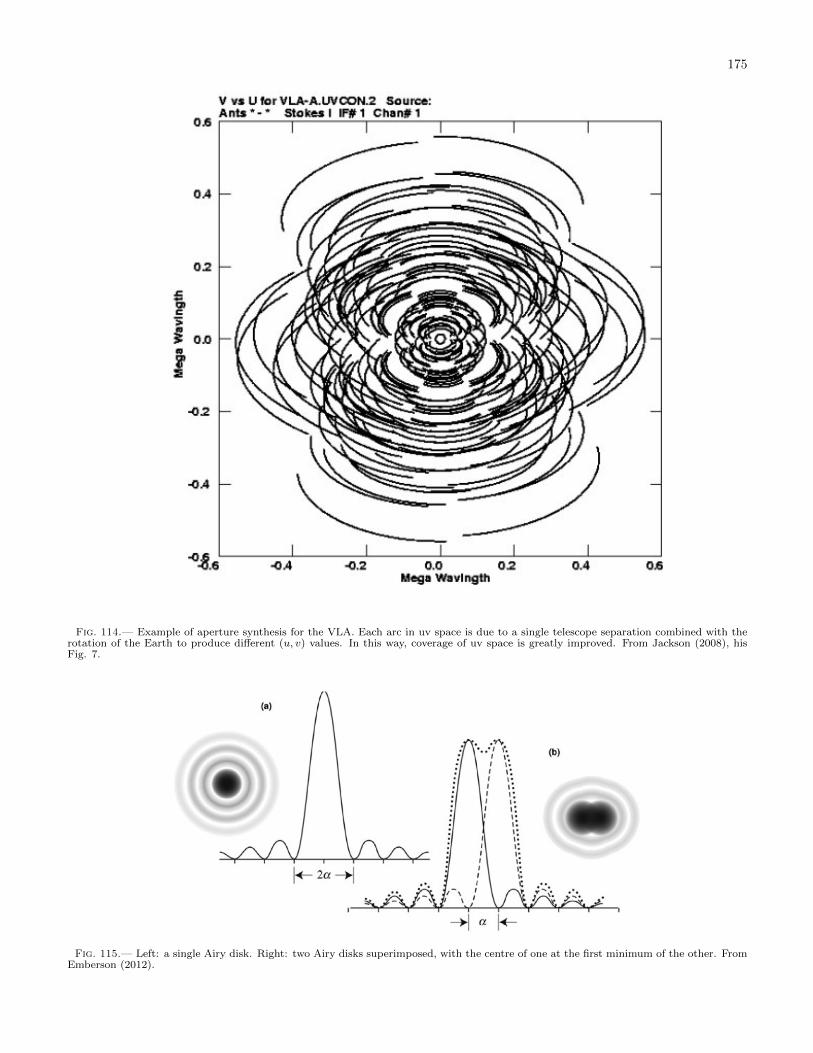
175

Fig. 114.— Example of aperture synthesis for the VLA. Each arc in uv space is due to a single telescope separation combined with therotation of the Earth to produce different (u, v) values. In this way, coverage of uv space is greatly improved. From Jackson (2008), hisFig. 7.

Fig. 115.— Left: a single Airy disk. Right: two Airy disks superimposed, with the centre of one at the first minimum of the other. FromEmberson (2012).

176

of this function can be seen in Fig. 115. The first minimum of this function occurs at

α ≈ sin(α) =1.220λ

2R=

1.220λ

D(222)

We note that the plane wave is the FT of a distant point source - if we had an infinite sized aperture and an infinitelens, our focal plane image would be the FT of an FT (i.e. roughly equivalent to an FT and then an inverse FT),convolved with the FT of the aperture. If two objects were to have an angular separation less than α, their Airydisks would begin to merge (Fig. 115). This blend is still distinguishable for θ < α, but this becomes very difficult,especially if one source is much less bright than the other. This is why we consider Eqn. 222 the diffraction limit (i.e.a resolution limit) of a telescope (also known as the Rayleigh criterion).

Earthbound telescopes often have a much more stringent limit set on it by turbulence in the atmosphere. Tem-perature gradients in the Earths atmosphere caused by turbulence create compressions and rarefactions in the airand correspondingly higher and lower indices of refraction. These regions in the air retard some sections of a planewavefront while allowing other sections to progress forward. For telescopes operating past the Fried coherence length

(the distance over which the phase difference is one radian) r0 ≈ 0.114(λ cos z

550

)0.6m (where z is the angle to the

zenith), the atmosphere sets up an seeing limit (Hickson 2002)

αeff ≈λ

r0(223)

which limits the resolution of the telescope (For telescopes smaller than this limit, atmospheric turbulence createsscintillation, or twinkling, hence why the stars twinkle to the naked eye.)

There can also be instrumental reasons for why a telescope is not operating at its diffraction limit. These includemirror/lens imperfections and inherent design features, such as the ones on the Chandra space telescope.

Three telescopes that are operating at the diffraction limit are:

• Giant Meterwave Radio Telescope (GMRT), which has an effective mirror diameter (since GMRT is anarray) of 25 km, operates on the GHz frequency and has a ∼ 2” resolution.

• The Hubble Space Telescope (HST), which has an aperture diameter of 2.4 m, works in the optical (∼ 500nm) and has a resolution limit of about 0.052”.

• The Spitzer Space Telescope, which has an aperture diameter of 0.85 m, works in the near-IR (8 µm), andhas a resolution limit of about 2”.

In general, space telescopes and radio telescopes operate at the diffraction limit. Three telescopes that do not operateat the diffraction limit are:

• Chandra X-ray Observatory, which has an aperture diameter of 1.2 m, looks at x-rays with wavelength 1 nmand has an angular resolution limit of 0.5”. This is due to imperfections in Chandra’s concentric mirror shells.

• W.M. Keck Observatory, which has a diameter of 10 m, looks in the optical (∼500 nm), but is seeing limitedto ∼1”. Adaptive optics decreases this limit almost to the diffraction limit.

• XMM Newton, with an effective diameter of 0.74 m, works in the x-ray, and has a resolution limit of about6”.

In general, high-energy telescopes and telescopes on the ground do not operate at the diffraction limit.

5.3.1. What if the lens or mirror is not perfect?

This information is from Hickson (2002) and Kitchin (2009), Ch. 1.1.17.2.A number of optical imperfections can distort images:

• Spherical aberration, where different areas of the spherical mirror/lens have different focal points.

• Chromatic abberation, where different wavelength light have different focal points.

• Coma, where a paraboloidal mirror/lens generates comet-like distortions.

• Astigmatism, where bar-like distortions are generated.

• Distortion, a variation of magnification across the image.

177

5.3.2. How does adaptive optics work? Does it truly create diffraction-limited images?

Adaptive optics (AO) can correct wavefront distortions that arise from atmospheric turbulence and sharpen blurredimages on long exposures. A guide star or laser artificial star is used as a reference to determine atmospheric distortions.A set of small, deformable mirrors or a lenslet array is then employed to correct the atmospheric distortions generatedfrom turbulence. This process is somewhat easier in the near-infrared because of the longer wavelengths involved. Asa result, AO have been successful in providing near-diffraction-limited images in the near IR.

Since AO is a complicated system, it generates its own intrinsic errors. Moreover, atmospheric turbulence cannotcompletely correct for atmospheric turbulence, since there is a delay in image correction, as well as a directionaldependence on turbulence. Solutions include more efficient computational algorithms and adding additional guidestars (ex. via multiple lasers).

5.4. Question 4

QUESTION: What’s the minimum mass of a black hole you could survive a fall through the eventhorizon without being ripped to shreds? Why would you be ripped to shreds for smaller black holes?

This is from Kissin (2012), with a little help from last year’s qualifier notes.We can approximate the black hole with a Schwarzschild metric. The event horizon is then

rBH =2GM

c2(224)

The Newtonian approximation for the tidal force per unit mass is

ft ≈dg

drL (225)

which is a fine approximation so long as dgdr >>

d2gdr2L. Calculating this nets us ft ≈ L 2GM

r3 . If we are at the eventhorizon of the black hole, then

ft ≈c6L

4G2M2. (226)

Solving for M , we obtain

M =

√c6L

4G2ft(227)

Traditional forms of execution include dismembering an individual through the tidal force of horses pulling in differentdirections. A very ballpark estimate suggests 100 g’s would tear a human limb from limb (horses pulling cannot bemore than 104 N, which translates, for a 100 kg person, into 100 g’s). If we also assume L ≈ 2 m, then we obtain amass M ≈ 1034 kg, or 5× 103 M.

From Eqn. 226, it is obvious that as mass decreases, the tidal force increases. This has to do with the Schwarzschildradius being dependent on mass, and the tidal force being dependent on M−3.

5.4.1. How are supermassive black holes (SMBHs) formed?

This is from Wikipedia (2012g) and Carroll & Ostlie (2006), pg. 639.This is still an open question. The most obvious hypothesis is that black holes of tens or perhaps hundreds of solar

masses that are left behind by the explosions of massive stars grow by accretion of matter. It is possible SMBHs couldhave formed from the collisions of galaxies. They could also have formed out of pre-galactic halos through variousinstabilities, culminating in the formation of a ∼ 10 M black hole, which then accretes at super-Eddingthon ratesuntil it reaches ∼ 105 M. Black holes could also have been formed from the Big Bang itself.

The primary unsolved issue today is how to feed these black holes until they reach SMBH status. The existenceof high-redshift quasars requires that SMBHs be formed soon after the first stars. No method is known to gorgeprimordial BHs to stimulate such rapid growth.

5.5. Question 5

QUESTION: Let’s say the LHC produces microscopic black holes in their high energy proton-anti-proton collisions? What will happen to them? Will they destroy the Earth?

178

This information comes from my own notes, buoyed with wikipedia (2012) and last year’s notes on the problem.If the LHC produces microscopic black holes, they will likely almost instantly decay through Hawking Radiation.

Black hole thermodynamics demands that a Schwarzschild black hole radiate like a blackbody with temperature

T =~c3

8πkBGM. (228)

This will be stated without proof, but a useful motivation is below. The total radiation from the black hole is then

L = 4πR2sσSBT

4, giving us L = 2σ~4c12

(8π)3k4BG

2M2 . Since only the rest mass of the BH can provide energy, L = −c2 dMdt .

We can then equate the two, integrating from the time t = 0 when the BH had M = M0 to time t = tev when M = 0:∫ 0

M0

M2dM = −∫ tev

0

dt (229)

where we have thrown a lot of constants into K. Integrating this, solving for tev and plugging in the numbers ofconstants, we obtain:

tev = 8.4× 10−17s(M/kg)3 (230)

For a 1 TeV black hole, we would obtain tev = 5× 10−88 s!We can make this a bit more difficult by assuming that the black hole can swallow nearby masses to stave off its own

death. The accretion rate is then dM/dt = fπR2sρv (from Γ = nσv, where Γ is the number of collisions per second),

where f is of order unity. We then require, to stave off death:

L/c2 =2σ~4c10

(8π)3k4BG

2M2= fπR2

sρv. (231)

If we then assume v ≈ c to minimize ρ, we calculate ρ = 4σ~4c13

(8π)4k4BG

3M3 = 1.8 × 10155 kg/m3 (i.e. much greater than

black hole densities)! In order to survive by accreting particles while travelling at the speed of light (any less and theρ goes up) through pure iron, the black hole would need an rest energy of ∼ 1042 GeV.

Even if we suppose all our theory above is wrong, and black holes can be produced by the LHC and surviveindefinitely, it is still unlikely they would destroy the Earth. The LHC collision of two 7 TeV proton streams isequivalent to a stationary Earth atom being struck by a 108 GeV cosmic ray, and the cutoff for cosmic rays is around1011 GeV. We would then expect to see microscopic black holes being produced all the time in our atmosphere. Theseblack holes would be fast-moving, but as they accreted charge drag from electrostatic effects would keep them trappedin massive objects such as the Sun. Unless these black holes could rapidly neutralize (the only known mechanisms fordoing this would also cause Hawking radiation), they would have destroyed the Sun and the Earth long ago.

Similar arguments can be made to eliminate the possibility of strangelets or magnetic monopoles destroying theworld.

5.5.1. Can the LHC produce microscopic black holes?

Not according to GR. The LHC produces an energy of 1 TeV within a length of 10−19 m. A black hole with aSchwarzschild radius 10−19 m would have a rest energy of 1035 GeV, far more than the LHC could produce.

5.5.2. What if there were more dimensions than 4 to the universe?

If there were extra spatial dimensions, the number of which is given by d (i.e. d = 0 for 4 dimensions), thenT ∝ M−1/(1+d). The temperature dependence on mass would therefore be shallower and it would take longer for theBH to evaporate. Current experiments with modified gravity at very small scales have shown d ≤ 2, and even withd = 2, our analysis above does not change substantially. The minimum rest energy a black hole must have to stave offthermodynamic death by accreting iron while travelling at the speed of light is ∼ 1024 GeV.

5.5.3. Can you motivate why temperature is inversely propotional to mass for black hole thermodynamics?

This information comes from Wayne Ngan’s notes on the problem.Suppose we have a black hole made of photons, and each photon has wavelength λ = Rs. The number of photons

within the black hole is then

N = Mc2λ/hc =2GM2

hc(232)

The entropy of the system is S = kB ln Ω ≈ kB ln(N !), and if N is large, ln(N !) ≈ N ln(N) − N . For a very roughorder of magnitude, say that ln(N)− 1 ∼ 1 (we will perhaps be an order of magnitude off). Then S ∼ E/T ∼ kBN ,and E = Mc2, which gives us

T ∼ hc3

kBGM=

~c3

8πkBGM(233)

179

5.6. Question 6

QUESTION: How is synchrotron radiation generated? In outline, how can it be removed from CosmicMicrowave Background maps?

This information is from Zhu (2010).Synchrotron radiation is generated by electrons looping inside magnetic fields. Suppose, without loss of generality,

that ~B is pointed along the z-axis. Then any electron caught in the field will travel along a trajectory ~r(t) =zvzt+

vxyωB

(x cos(ωt)+ y sin(ωt)), with ωB = eBγmc . As this electron loops inside the magnetic field at relativistic speeds,

it tends to generate highly beamed emission. This emission comes at the frequency at which the electron orbits alongthe magnetic field, ω = 3

2γ3ωB sinα = 3

2γ2ωL sinα, where ωL is the Larmor frequency, and α is the pitch angle,

between the projection of the vector ~v onto the xz or yz plane, and the magnetic field. If we Fourier transform thesquare of the electric field, we get the emission spectrum. If we then assume a power law distribution with index p(i.e. n(γ) = n0γ

−pdγ), the total emission becomes a power law,

Iν ∝ ν−(p−1)/2. (234)

If the region is sufficiently dense with electrons, synchrotron self-absorption sets in, and the low ν end of the spectrumis given a power law ν5/2 (the frequency at which the spectrum transitions back to a power law is dependent on themagnetic field). In galactic emission p is often about 8, giving Iν ∝ ν3.5. See Fig. 117.

Note that synchrotron is highly polarized. This is because emission is always orthogonal to the direction of the field.This means a measure of synchrotron polarization allows us to measure the direction of the magnetic field (projectedonto the sky).

Fig. 116.— Schematic of how synchrotron radiation is derived. Upper left: electric field from a single electron in a magnetic field. Bottomleft: Fourier transform of E2 from a single electron. Upper right: emission from a distribution of electrons (all FT’ed). Bottom right: thefull spectrum, taking into account self-absorption at low frequency. From Marleau (2010), Lecture 6.

See Sec. 1.13 for information on how synchrotron radiation is removed from the CMB.

5.6.1. What is cyclotron radiation?

This information is from Rybicki & Lightman (1979), pg. 182The non-relativistic limit of synchrotron radiation is cyclotron radiation, which occurs when the electrons are not

180

moving relativistically. The emission spectrum from a single electron is then a delta function given by the frequency

f =qB

mc. (235)

This means that, even moreso than synchrotron radiation, cyclotron radiation traces the distribution of electronenergies in the gasy. Cyclotron is polarized.

5.6.2. What are common sources of synchrotron radiation?

Essentially anything with a strong magnetic field and free electrons nearby will radiate synchrotron emission. Sourcesinclude AGN jets, supernova remnants, pulsar wind nebulae.

5.6.3. What do the spectra of other major radiation sources look like?

• Blackbody radiation

• Bremsstrahlung

• Thomson scattering

• Compton scattering

5.7. Question 7

QUESTION: What are ”forbidden lines” of atomic spectra? In what conditions are they observa-tionally important?

This comes from Draine (2011), pg. 60 - 62, and Griffiths (2005) Ch. 9.2.Spontaneous emission comes in two camps: allowed and forbidden, which simply indicates the strength of the

transition. The strength can be calculated using time-dependent perturbation theory (Griffiths (2005), Ch. 9.2). Wefirst determine stimulated emission and absorption by looking at a two-level system being perturbed by the Hamiltonian

H ′ = −qE0z cos(ωt), (236)

recalling that corresponds classically to V = −qEz, i.e. if the electric field is uniform, V is a linear function ofposition, and we orient the z-axis to the movement of the electron. As it turns out, this means that the probabilityof transitioning between the states, Pab = Pba ∝ 〈ψa|r|ψb〉. These are stimulated transition probabilities, but bythe nature of Einstein’s coefficients, it means that the spontaneous transition probabilities also depend on 〈ψa|r|ψb〉.Because 〈ψa|r|ψb〉 looks a little like a dipole moment, this is known as electric dipole radiation.

As it turns out, there are large numbers of different states a and b for which 〈ψa|r|ψb〉 is zero. We have made anapproximation in Eqn. 236, which is that the electric field is uniform over space. In general E(r, t) = E0 cos(k ·r−ωt),and we can expand this out into E(r, t) ≈ E0(cos(ωt) + k · r sin(ωt)). The first term give electric dipole transitions,while the second gives electric quadrupole transitions and magnetic dipole transitions. These transition probabilitiesare substantially weaker, and therefore spontaneous emission due to electric dipole, or allowed, transitions, occurs ata much more prolific rate than spontaneous emission due to quadrupole or magnetic dipole, or forbidden, transitions.

Allowed transitions must follow the following rules:

1. Parity must change. Parity is defined as∑i li (i.e. adding the angular momentum quantum number of all

electrons) and can either be even or odd.

2. Change in total angular momentum ∆L = 0, ±1.

3. Change in total angular plus spin momentum ∆J = 0, ±1, but J = 0→ 0 is forbidden.

4. Only one single electron wavefunction nl changes, with ∆l = ±1.

5. Total spin ∆S = 0 (spin cannot change).

Allowed transitions are denoted without square brackets. There are transitions that follow all these rules except thelast, and are known as semiforbidden, intercombination, or intersystem transitions. These are denoted with squarebrackets only on the right. Forbidden transitions break any rules from 1 to 4, and are denoted with square brackets.Roughly speaking, semiforbidden lines are 106 times weaker than allowed transitions, and forbidden lines are 102−106

times weaker than semiforbidden lines. I believe magnetic dipole transitions are stronger than electric quadrupoletransitions.

Because they are so much weaker, forbidden lines are easy to collisionally wash out at high densities. In the ISM andaround certain stars, however, it is possible to have extremely tenuous gas, and in these gases forbidden transitionsbecome important. Indeed, forbidden line emission that have different critical densities ncrit at which they begin tobe suppressed can be used as density diagnostics. (Forbidden lines can also be used as temperature diagnostics, whichmeans that density effects must be accounted for when performing calculations. See Sec. 3.17.)

181

5.7.1. Derive Einstein’s coefficients.

This comes from Hickson (2002).Suppose there are two states 1 and 2 in a system at thermodynamic equilibrium; this means that

n1B12J = n2(A21 +B21J), (237)

where Bab represents stimulated transition between a and b, Aab represents spontaneous emission, and J represents theintensity of photons at the correct frequencies to drive transitions. Since the system is in thermodynamic equilibrium,

n2

n1=g2

g1e−hν0/kBT , (238)

where ν0 is the wavelength difference between states 1 and 2. Moreover, a system in thermodynamic equilibriumradiates as a blackbody, so J ≈ Bν(ν0) (the ≈ is because there is some variation in ν over a line profile, but thisvariation is small). Combining Eqns. 237 and 238 gives us

Bν(ν0) =A21/B21

g2B21

g1B12ehν0/kBT − 1

, (239)

and comparing this to the Planck spectrum gives us:

g1B12 = g2B21

A21 =2hν3

c2B21. (240)

B can be calculated from time-dependent perturbation theory.

5.7.2. How do atoms end up in states where they can only transition back out through a forbidden line?

Atoms can either be collisionally exited into the state, absorb a photon with the right frequency (both collision andabsorption could happen multiple times before the atom returns to the ground state), or cascade down from a higherenergy state and become “trapped”.

5.8. Question 8

QUESTION: What is a polytropic equation of state? Give examples of objects for which this is avery good approximation.

Most of this answer is from Kissin (2012), with help from last year’s qualifier notes and Kippenhahn & Weigert(1994).

In general, the equation of state for a gas has the form P = f(ρ, T ), i.e. pressure is a function of both density andtemperature. This is analytically difficult to work with, since there are essentially two free parameters and setting Pcannot uniquely determine both ρ and T . In many situations, however, T is a function of ρ, and in these situationsP = f(ρ), known as a barytropic equation of state. A subset of these equations of state, where

P = Kργ = Kρ1+1/n (241)

are known as polytropic equations of state. γ is known as the polytropic exponent, K the polytropic constant and nthe polytropic index. K can either be fixed (as we will see below) or remain as a free-parameter that varies from starto star.

Of course, in many situations polytropes are not realistic equations of state. Examples of where they are include:

1. Radiation-dominated stars: consider the total pressure in a region of a star to be the sum of the gas kineticpressure and the radiation pressure, i.e.

P =kBµmH

ρT +a

3T 4 =

kBµmHβ

ρT (242)

where β = Pideal/P . Then 1− β = Prad

P = aT 4

3P . We can then replace temperature with a function of pressure toget

P = Kρ4/3 =

(3k4B

aµ4m4H

]

)1/3(1− ββ4

)1/3

ρ4/3, (243)

182

which is an n = 3 polytrope, if β is constant. Extremely massive stars are nearly completely radiation-dominated,completely convective (i.e. roughly isentropic), which for radiation means ρ ∝ T 3; combining this with P ∝ T 4

nets us γ = 4/3, which is an n = 3 polytrope and consistent with our prior derivation. The Sun can beapproximated by an n = 3 polytrope, though the match would not be perfect since the Sun has a convectiveenvelope.

2. Zero-temperature degenerate stars: these are considered in detail in Sec. 5.12. Suffice it to say, a non-relativistic completely degenerate gas has P ∝ ρ5/3 and a relativistic completely degenerate gas has P ∝ ρ4/3.An n = 3 polytrope is inherently unstable, and that manifests itself here in a maximum mass for degeneratestars. The non-relativistic equation works well for cold white dwarfs, brown dwarfs, and gas giants.

3. Adiabatic stars: consider an ideal gas with 2α degrees of freedom. Then U = αNkBT = αPV . The first lawof thermodynamics then says dU = −PdV . Substituting dU = αPdV +αV dP , we obtain dP

P = −α+1α

dVV , which

nets us

P ∝ ρ(α+1)/α. (244)

For a monotonic gas, α = 3/2, giving γ = 5/3, or n = 3/2.

4. Isothermal stars: this is obvious: P ∝ ρ, with K = kBTµmH

. True isothermal stars do not exist, but this can give

the structure of the inert core of a shell-burning star.

5.8.1. Why are polytropes useful?

The advantage of using a polytropic equation of state is that it immediately simplifies the equation of hydrostaticbalance dP

dr = −dΦdr ρ into

dΦ

dr= −γKργ−2 dρ

dr. (245)

This can be integrated to obtain ρ =(−Φ

(n+1)K

)nif γ 6= 1 and we have set Φ = 0 when ρ = 0. The Poisson equation

assuming spherical symmetry reduces to

1

r2

∂

∂r

(r2 ∂Φ

∂r

)= 4πGρ. (246)

We can then substitute in ρ. We now define z = Ar, where A2 = 4πG(n+1)K ρ

1−1/nc and w = Φ

Φc=(ρρc

)1/n

, where

subscript c refers to central values. We may then rewrite Eqn. 246 as

d2w

dz2+

2

z

dw

dz+ wn = 0. (247)

This is known as the Lane-Emden equation. Since it is equivalent to 1z2

ddz

(z2 dw

dz

)+wn = 0, to prevent w(z = 0) =∞,

we set dwdz (z = 0) = 0.

While there are only a few analytical solutions, this is a relatively easy integral to solve (to remove the regularsingularity at zero we may expand w(z) into a power series). We are then able to determine the density ρ as a functionof the central density as a function of radius.

To scale this solution to a star, we use the relation

M = 4πρcR3

(−1

z

dw

dz

)z=zn

(248)

If we do not fix K, then all we need to specify are n and two out three variables, M , R, and ρc. If we do fix K,then all we need to specify are n and one out of M , R, and ρc. Fixing K naturally gives the mass-radius relationshipR ∝M (1−n)/(3−n).

5.8.2. What numerical methods are used to for calculating polytropes?

A brief description of shooting goes here.

5.8.3. How is the Chandrasekhar Mass estimated using polytropes?

With electricity and meat.

183

Fig. 117.— Results from integrating the Lane-Emden equation for a given polytrope. Integration ends when z = zn, at which pointw(z) = 0. From Kippenhahn & Weigert (1994), their Table 19.1.

5.9. Question 9

QUESTION: What was the solar neutrino problem, and how was it resolved?

This answer is from Carroll & Ostlie (2006), pg. 356 - 360.The solar neutrino problem was first discovered by Davis et al. in 1970. Davis et al.’s neutrino detector at Homestake

Gold Mine in South Dakota contained approximately a thousand metric tonnes of cleaning fluid, C2Cl4, in order toobserve the weak reaction

3717Cl + νe

3718 Ar + e−. (249)

3718Ar has a half-life of 35 days. The threshold energy for this reaction is less than the energies of the neutrinos producedin every step of the pp-chain save for the first (1

1H+11 H→2

1 H+e+ +νe), though most of the neutrinos detected shouldbe from

85B→8

4 Be + e+ + νe. (250)

Careful calculations of solar neutrino emission and reaction with C2Cl4 suggested that 7.9 Solar Neutrino Units (SNU,defined as 10−36 reactions per target atom per second) should be recorded in the Homestake experiment. The actualdata gave 2.56± 0.16 SNU. This was corroborated by other detectors, such as Japan’s Super-Kamiokande (which usespure H2O surrounded by detectors; neutrinos scattering off electrons produce Cherenkov radiation, which can thenbe detected) and the Soviet-American Gallium Experiment and GALLEX in Gan Sasso, Italy (which use the reactionνe +71

31 Ga→7132 Ge + e−).

The resolution to this deficit of neutrinos, known as the solar neutrino problem, is known as the Mikheyev-Smirnov-Wolfenstein (MSW) effect, which involves the transformation of neutrinos from one flavour to another. All neutrinosproduced by the Sun are electron neutrinos (νe), but during their journey from the Sun to Earth they oscillate betweenelectron, muon (νµ) and tau (ντ ) neutrinos. All experiments reporting a neutrino deficit were sensitive only to νe.

In 1998 Super-Kamiokande was used to detect atmospheric neutrinos produced when high-energy cosmic rays collidewith Earth’s upper atmosphere, which is capable of creating electron and muon neutrinos, but not tau neutrinos. Theyfound that the muon neutrino flux coming from underneath the detector was substantially less than the flux comingfrom overhead. This can be interpreted as muon neutrinos generated on the other side of the planet oscillating intotau neutrinos on their way to the detector, while the muon neutrinos generated on the near side of the planet havenot had the time to do so. The Sudbury Neutrino Observatory has been able to detect all three flavours of neutrino.

5.9.1. Why do we believe neutrinos have masses?

This answer is from Carroll & Ostlie (2006), pg. 359, and Schneider (2006), pg. 351 - 352.One testable consequence of the MSW effect was that flavour oscillation was only allowed by grand unified theories

if neutrinos had mass (electroweak theory does not predict neutrinos to have mass). The current established upperlimit for neutrino masses is around 0.3 eV, which is still greater than the mass needed for the MSW effect to operate.

Experimentally, neutrino mass can be determined via particle accelerator experiments, which have set a lower limitfor the total neutrino mass of all three flavours to be ∼ 0.05 eV. Since neutrinos are considered hot dark matter,they suppress both the CMB power spectrum and the matter power spectrum at small scales by free-streaming. AnΩνh

2 < 0.0076 implies that the maximum neutrino mass is < 0.23 eV.

184

5.10. Question 10

QUESTION: Why is nuclear fusion stable inside a main-sequence star? Under what conditions isnuclear fusion unstable? Give examples of actual objects.

This answer is from Kippenhahn & Weigert (1994), Sec. 20.3 and 25.3.4, as well as van Kerkwijk (2011).Nuclear fusion inside main sequence stars is stable due to the “solar thermostat”. Suppose fusion inside a star

increases on a local thermal adjustment timescale. The thermal energy generated by the increases the temperature,which, by the ideal gas law, generates an overpressure. The system is no longer in hydrostatic equilbrium and the starexpands. Since work is done during this expansion, the star must then cool, which quenches any increase in fusionrate due to increase in temperature. The star then relaxes back into its previous equilibrium.

This is actualy something that can be determined from the virial theorem, which holds if the star is in hydrostaticequilibrium. 2Ei = −Eg requires that if the star expands, and therefore its in

The following two equations are derived in more detail in Sec. 20.3 in Kippenhahn & Weigert (1994), but here we

perform an order of magnitude scaling. Density for a star is given by ρ ∝M/R3, and mass is fixed, so ρ/ρ = −3R/R.

For the same reason (P ∝M2/R4) we obtain P /P = −4R/R. If our system expands and contracts homologously, the

same equations hold for any radius r (and so ex. P /P = −4r/r). Lastly, we assume an equation of state ρ ∝ PαT−δ;taking the total differential gives us ρ/ρ = αP/P − δT /T . Since ρ/ρ = −3R/R, we obtain T /T = −((4α− 3)/δ)r/r.To summarize:

ρ

ρ= −3

r

r

P

P= −4

r

r

ρ ∝ PαT−δ

T

T= −4α− 3

δ

r

r(251)

For an ideal gas α = δ = 1, so we immediately see

T

T= − r

r(252)

i.e. an increase in temperature drives an outward, homologous expansion, which by this equation requires a decreasein temperature. Indeed, we can also derive P /P = if we use the first law of thermodynamics (dQ = dU + PdV ) andadjust it to our system (dQ = cP dT − δ

ρdP , ∇ad = PδTρcP

; see Kippenhahn & Weigert (1994), Eqns. 4.18 and 4.21), we

can derive the heat capacity of a star

c∗ = cP (1−∇ad)4δ

4α− 3, (253)

which is negative for an ideal gas. This is equivalent to our derivation from before (though perhaps less, since it statesthat an increase in fusion rates results in a decrease in temperature. Note that Kippenhahn & Weigert (1994) Sec.25.3.4 adds c (“central”) to all its variables; this is to denote that we are supposing homologous expansion properlydescribes changes in central values.

Examples where nuclear fusion is unstable:

• Thin shell source: when the centre of a star becomes too cold for nuclear fusion, fusion continues in a shellaround an inert core. Since the temperature on the inside of the shell is hotter than on the outside, which affectsfusion rate, the shell thins over time. A thin shell homology a distance r0 from the centre of the star has masswithin the burning shell as m ≈ ρr2

0D; assuming mass is fixed, this translates to ρ/ρ ∝ −D/D = −(r/D)r/r

(since r = r0 +D). Performing the same calculation as before using P /P = −4r/r and the equation of state, we

obtain TT =

(rD − 4

)rr . If D < r/4, an expansion actually increases temperature. This leads to thermal pulses

on the asymptotic giant branch.

• Central fusion in a degenerate equation of state: for a non-relativistic degenerate object, δ = 0 andα = −3.5, so from Eqn. 253 the heat capacity is positive. Equivalently, Array 251 shows that pressure isindependent of temperature. This means in a degenerate object pressure does not increase with temperature.Since there is no cooling mechanism, and temperature increases fusion rates, this is a nuclear runaway. Thismechanism destroys white dwarfs in SNe Ia.

185

• Faster than dynamical nuclear fusion: a star can be unstable in any situation where the nuclear burningrate becomes faster than the dynamical time, since the star no longer has the ability to readjust its structureto compensate for the increasing energy. An example of this is a pair-instability supernova: stars that produceoxygen cores of & 40 M (these stars are > 100 M and could be prototypical Pop III stars) will, on their wayto producing iron, begin producing electron-positron pairs. This creates a γ < 4/3 equation of state inside thestar (energy is being siphoned off to produce pairs), and the star collapses until carbon fusion is ignited on atimescale less than the dynamical time, and destroys the star.

5.10.1. Why does the star expand homologously?

It actually does not, but homologous expansion is a useful approximation to make the derivation of fusion stabilityand negative heat capacity tractable.

5.10.2. What if you increased fusion tremendously inside a star? Would that not destroy it?

It would. Another factor to why a star is stable to nuclear fusion is that changes to fusion occur on a thermaladjustment timescale in main-sequence and giant stars (for the most part), and therefore hydrostatic equilibrium ismaintained. An example of when it is not is listed above: the pair-instability supernova.

5.11. Question 11

QUESTION: Why do neutrons inside a neutron star not decay into protons and electrons?

This information is from Townsend (1997).Degeneracy pressure is physically generated by forcing electrons into increased momentum states so as to satisfy the

Pauli exclusion principle - the quantization of phase space requires that electrons sharing the “same” position musthave different momenta. As such, an increased compression generates a higher distribution of momentum states (i.e.the top of the Fermi sea, given by energy EF , is higher).

The mass of a neutron is 1.001378 the mass of a proton, and the mass of an electron is 5.44617× 10−4 the mass ofa proton (Wolfram 2012). Electron capture,

e− + p+ → n+ νe (254)

therefore requires about 8 × 10−4mpc2 worth of kinetic energy in the reactants, approximate the same value as the

rest energy of the electron. When the neutrino energy is accounted for, approximately 3 times the rest energy of theelectron is needed.

For ordinary (even relativistic) WDs, EF . mec2, so WDs are stable to electron capture. A collapsing WD, however,

will increase its EF to infinity (at infinite EF there is still insufficient electron degeneracy pressure to halt collapse,since there are still tons of low-energy electrons), making electron capture possible.

Once electron capture occurs, it cannot come into equilibrium with the reverse reaction (“assisted beta decay”,n+ νe → e−+ p+) because the neutrino escapes the WD. Beta decay (n→ e−+ p+ + νe) can can occur, however, anddo, to the point at which EF filled to ∼ 3mec

2 when inverse beta decay becomes ENTROPICALLY? preferred. Thismakes it so that in the regime of nuclear saturation density (i.e. the nucleons “touch”; ∼ 3×1014 g/cm3) electrons andprotons still make up ∼12% of the material (van Kerkwijk 2012). Neutrons, however, dominate, since EF is rapidlyfilled at neutron star densities. The limiting value, set by the balance between beta decay and electron capture andmediated by filling the electron Fermi sea, is 8 neutrons to 1 proton and 1 electron (Carroll & Ostlie 2006, pg. 581)

It is therefore not entirely true that neutrons do not decay into protons and electrons, but a neutron star is stableto beta decay.

5.12. Question 12

QUESTION: Give examples of degenerate matter.

This is from my own notes and Kippenhahn & Weigert (1994), Ch. 15.Degenerate matter is matter in which pressure due to the Pauli Exclusion Principle dominates over pressure calculated

from the ideal gas. (Partly degenerate matter is when the two are on the same order of magnitude, indicating thermalpressure support still plays a significant role.) This pressure comes from two factors. The first is that in quantummechanics the number of possible states in phase space is discretized; this “density of states” can be calculated by,for example, determining the discretization of eigenstates in an infinite square well, and then taking the boundariesof this well to infinity (Sturge 2003). The second is the Pauli Exclusion Principle, which prevents the occupation of asingle phase space state by particles with the same spin. For a gas of electrons and neutrons, for example, this resultsin

f(p)dpdV ≤ 8πp2dpdV/h3 (255)

186

where f(p) is the “occupation number” of a state p, and runs from 0 to 1. As lower p values become full (f(p) = 1),electrons and neutrons are forced to occupy higher p states - this is what generates degeneracy pressure. In a completelydegenerate gas, the highest p state is known as the Fermi momentum, and its associated energy the Fermi energy.Since the momentum (equivalently the energy) is nonzero, the Fermi momentum and energy are associated with aFermi pressure. In a partly degenerate gas, there is no critical value of p, though the fact that f(p) ≤ 1 can still havean effect on the overall pressure.

Examples of degenerate matter include:

• Electron degenerate matter - in white dwarfs, massive gas giants and brown dwarfs, as well as within post-main sequence stars.

• Neutron degenerate matter - in neutron stars.

More theoretical forms of degenerate matter include:

• Proton degenerate matter - is physically possible, but practically it is always overshadowed by electrondegeneracy due to its much larger Fermi sea - the only way for proton degeneracy to become prominent is tohave an object completely made of protons.

• Quark degenerate matter (QCD matter) - at T ∼ 1012 K or densities where the average inter-quarkseparation is less than 1 fm (or a combination of both), hadrons will tend to decompose themselves into quarks.This matter will be Fermi degenerate, but will also exhibit properties such as color superconductivity.

• Preon degenerate matter - if quarks and leptons themselves are comprised of sub-components, we wouldexpect them to break up at extremely high temperatures and pressures. Under these conditions degeneracypressure of the sub-components (called preons) could hold the system against gravitational collapse.

5.12.1. How can you tell if something is degenerate?

For a Fermi gas, the more general equation for the occupation of states is

f(p)dpdV =8πp2dpdV

h3

1

1 + eE/kBT−ψ(256)

where ψ =∞ at infinite density or zero temperature, and ψ = −∞ at infinite temperature or zero density. From theargument in pg. 124 of Kippenhahn & Weigert (1994), for a non-relativistic gas,

ψ = ln

(h3n

2(2πmekBT )3/2

)(257)

and the degeneracy/non-degeneracy limit is approximately when ψ = 1. An easier way of determining degeneracylines on a ρ− T diagram is to use the degeneracy parameter:

EFkBT

. (258)

This value is ∝ n2/3/T for non-relativistic gases, and ∝ n1/3/T for a relativistic gas.

5.12.2. Why are white dwarfs composed of an electron gas (rather than, say, a solid)? Are WDs pure Fermi degenerate gases?

In WDs, the gas is of sufficiently high density that it is nearly fully pressure-ionized.WDs are not perfect zero-temperature Fermi gases. The first correction that must be made, especially for hotter

> 108 K WDs is that f(p) does not have to be either 0 or 1, as is the case for a zero-temperature Fermi gas. Thisadds a (. 10%) thermal pressure component to the gas. The second correction that needs to be made is the ions inthe system. From above, if ψe ≈ 1 for electrons in the system, ψ >> 1 for the ions, and as a result the ions are notdegenerate even when the electrons are, and contribute a negligible amount of pressure (this, by the way, is true evenif the ions are degenerate; see Sec. 4.14). At high densities and particularly low temperatures, ions have a tendency

to form crystal lattices; this occurs when (Ze)2/rionkBT ≈ 1, which means that it is proportional to n1/3ion /T . This

has no real effect on the overall pressure of the system, which is still dominated by degeneracy pressure, but it is anadditional source of energy for cooling WDs.

5.12.3. Sketch the derivation of the Fermi pressure.

Recall from Sec. 4.14 that we get pF for zero temperature perfect Fermi gas from:

n =

∫ pF

0

f(p)dp (259)

187

where f(p) = 8πp2

h3 - the reason this is true is because f(p) describes the number of filled states per momentum rangedp that fit in volume dV . (Note we can derive EF from pF through EF = pF /2m for non-relativistic and EF = pF cfor relativistic.) The energy density is then

u =

∫ pF

0

E(p)f(p)dp (260)

where E = p/2m if the gas is not relativistic, E = pc if the gas is completely relativistic, and E = mc2√

1 + p2

m2c2 in

general. The pressure is similarly derived: the pressure is simply the net momentum flux through an area dσ (see pg.120 of Kippenhahn & Weigert (1994)) and therefore

P =1

4π

∫2π

∫ ∞0

f(p)v(p)p cos2 θdpdΩ =1

3

∫ pF

0

f(p)v(p)pdp, (261)

where we have used the fact that the flux should be isotropic. We note v(p) = p/m√1+p2/(mc)2

in general, and that

v = p/m in the non-relativistic limit, and v = c in the relativistic limit. Our results, then, are:

P =1

20

(3

π

)2/3h2

mn5/3, (262)

for a non-relativistic gas, and

P =

(3

π

)1/3hc

8n4/3. (263)

for an relativistic gas. We can add subscript-e to mass and number density for electrons, or m for neutrons.

5.13. Question 13

QUESTION: What is the typical temperature of matter accreting on a star, a white dwarf, a neutronstar, a stellar mass black hole, and a supermassive black hole? In what wavelength range would onebest find examples of such sources?

This question is a streamlined version of pgs. 662 - 665 of Carroll & Ostlie (2006), with some help from last year’squalifier notes.

The question is not very specific about whether or not matter is being accreted spherically or onto a disk. We willassume it is a disk in our calculations, since in most physical circumstances the infalling material will retain angularmomentum.

Assuming virialization, the energy lost due to a particle being accreted is (assuming it started very far away)

E = −GMm

2r(264)

We may obtain dE/dr by differentiating. The amount of energy lost when a particle moves a radial distance dr isthen GMm

2r2 dr, where m is the accretion rate through the slice dr. Because an accretion disk accretes through viscousevolution, the energy is turned into heat (we have already assumed virialization in Eqn. 264, so there is no need toconsider rotational energy; also note material, as it streams down the accretion disk, is virial at all times with thisformulation). Now we shall assume steady state. Then for a slice of material dr, the difference in energy that passesthrough its outer and inner boundaries per unit time must equal to its luminosity (otherwise energy would pile up indr44). Then,

dLring = GMM

2r2dr = 4πrσSBT

4dr, (265)

noting that with steady state m = M for all dr. This gives us

T =

(GMM

8πσSBR3

)1/4(R

r

)3/4

, (266)

44 You may protest that dE/dr could simply go into heating the infalling material instead of being radiated, but recall that we requirethe disk to be completely virial at all times, requiring the total energy to be Eg/2. dE/dr is then the excess energy generated during theinfall.

188

noting that R cancels in the equation. For our question, we will set r = R. We may now perform some calculations.

• A white dwarf recurrent nova has a mass 0.85 M, radius 0.0095 R and accretion rate of perhaps 10−9

M/yr. This gives a temperature in the inner disk of 6.5 × 104 K, and a peak wavelength of 45 nm, which is

in the hard UV. Accreting WDs will emit in the ultraviolet (actually steadily accreting WDs with M = 10−7.5

emit in the soft x-rays).

• A neutron star with a disk has a mass 1.4 M, radius 1.5 × 10−5 R (10 km) and the same accretion rate.This gives us a temperature in the inner disk of 9.3× 106 K, and a peak wavelength of 0.31 nm, which is in thex-rays.

• A stellar mass black hole with a disk has a mass 5 M, radius 2.1×10−5 R (∼10 km) and the same accretionrate. This gives us a temperature in the inner disk of 9.9× 106 K, and a peak wavelength of 0.29 nm, which isin the x-rays.

• A supermassive black hole with a disk has a mass 108 M, radius 430 R and an accretion rate of 3 M/yr(Carroll & Ostlie 2006, pg. 1112). This gives us 5.1× 105 K, and a peak wavelength of 5.7 nm, which is in thesoft x-rays.

5.13.1. How will your results change if accretion was spherical?

This is something I thought up myself, with support from Spruit (2010), so read with a grain of salt.If we assume the accretion is spherical, then it is also infalling with spherical symmetry. The accreting material is

therefore in free fall until it strikes the surface, and becomes shock heated. For there to be equilibrium, the temperaturemust be below the effective temperature at the Eddington luminosity, Eqn. 160. If this is the case, then

GMM

R= 4πR2σSBT

4. (267)

We can then solve for T . This is not the temperature gained by a single particle being shock heated after gainingGMm/R worth of gravitational energy! Except for one particular M , the temperature T will be lower or higher

than 2GMµmH3RkB

. This is because while instantaneously infalling particles do get shock heated, the actual shock heating

energy gets spread across the surface, and at equilibrium (when energy into the system is equal to energy out of it),the total energy piled up on the surface creates a temperature such that the luminosity balances the incoming energyfrom falling material. A reasonable assumption is that M is indeed the Eddington accretion rate, in which case

T =

(LEdd

4πR2σSB

)1/4

=

(nneGMmpc

R2σTσSB

)1/4

(268)

5.13.2. What is Bondi accretion?

This information comes from Wikipedia (2012b).

An object plowing through the ISM will accrete at a rate M = πR2ρv, where ρ is the ambient density and v iseither the speed of the object (if subsonic) or the soundspeed cs if supersonic. R is not the radius of the object, but

the radius at which√

2GMR = cs. This accretion, known as Bondi accretion, would then occur at

M =4πρG2M2v

c4s(269)

5.14. Question 14

QUESTION: The weak equivalence principle for gravity corresponds to being able to find a coordinatesystem for a region of spacetime. What kind of coordinate system is this, and why?

This is cribbed off of Kissin (2012), with assistance from Dyer (2010a).The weak equivalence principle states that all laws of motion for freely falling particles are the same as in an

unaccelerated coordinate system or reference frame45.In general relativity, the motion of objects is given by the geodesic equation,

xe + Γembxmxb = 0, (270)

45 This is sometimes described as “the world line of a freely falling test body is independent of its composition or structure”. If a seriesof test bodies comprised various tests of the laws of motion were crammed into a small enough area, they would all follow (almost) thesame world line, and therefore all tests would be consistent with an unaccelerated reference frame.

189

where x is the 4-vector of an object, and overdots represent derivation with respect to an affine parameterization(equivalent to the proper time of the object). If we wish to find an unaccelerated reference frame, we equivalentlywant to find a coordinate system in which

xe = 0 (271)

i.e. the rate of change of coordinate time and space with respect to the proper time of the object is zero (i.e. noaccelerations). It can be shown (Dyer 2010a) that at point P a coordinate system can always be constructed suchthat Γemb is zero in the coordinate system. The coordinate curves are themselves locally geodesics (i.e. “in free fall”),and an observer fixed in these coordinates has no forces acting on them from gravity (in the Newtonian sense). Anyexperiments performed would find the same laws of motion as an unaccelerated reference frame, or inertial coordinatesystem.

Therefore, the weak equivalence principle corresponds to being able to find the locally geodesic coordinate systemat point P for which Γemb = 0, because Γemb = 0 translates to xe = 0, which translates to an local motions of objectsfollowing the same trajectories as if they were in an unaccelerated coordinate system.

In special relativity, it was possible to single out a special set of frames (inertial frames), and define mechanical andelectromagnetic forces as causing acclerations in these frames. With gravity, however, it is always possible to find somelocally inertial frame in which any “force” due to gravity is non-existent. This motivates the concept that gravity is ageometric effect, rather than a force in the same sense as an electromagnetic or mechanical force.

5.14.1. What is the significance of only being able to find this coordinate system at P?

Because the coordinate system is only geodesic in a small non-empty neighbourhood around P , as we move away fromP , the coordinate curves begin to diverge from the geodesics. Indeed, the only place where xe is zero is exactly at P !This is why even in the free-falling frame only experiments that are local (within the small, non-empty neighbourhood)are negligibly affected by the curvature of spacetime.

5.14.2. What is the strong equivalence principle?

The strong equivalence principle states that all laws of physics (rather than just the equations of motion that wedealt with above) that hold in Special Relativity hold exactly the same in a local inertial frame. This is equivalent tostating that a marriage of GR and electrodynamics, quantum and particle physics must reduce to their SR forms inthe free-falling frame, i.e. the influence of gravity on any physical process can locally be transformed away.

5.15. Question 15

QUESTION: What are the typical detectors used in gamma-ray, X-ray, UV, visible, infrared, sub-mm,and radio observations?

This information comes from Karttunen et al. (2007), Kitchin (2009) and last year’s qualifier notes.Commonly used detectors include:

• Charge-coupled device (CCD): a surface made of light-sensitive silicon (semiconductor) diodes, arrangedin a rectangular array of image elements or pixels. A photon hitting the detector ejects an electron into aconduction band (and produces an electron “hole” in the valence band). This electron is then trapped in thediode’s potential well until it comes time for readout. Readout occurs in the manner suggested by Fig. 118. Thequantum efficiency of CCDs is in the 70 - 90% range (highest in the infrared). The range of CCDs excends fromthe near-IR to the UV, though leftward of 500 nm the sensitivity drops due to absorption of UV radiation bysilicon. To correct this the chip is made thinner to reduce absorption, or a coating is applied to down-scatterUV photons to the optical. In the x-rays it is also possible to use CCDs (the absorption issue being specificto UV), though because of the high energies involved multiple electrons are ejected per photon. To minimizedark current (thermal noise), CCDs are cooled. CCDs have a maximum storage capacity, past which it becomessaturated

• Photomultiplier: a series of charged plates. Radiation hits the cathode, and releases electrons via the photo-electric effect. The electrons are then accelerated by an electric field until they strike a dynode, which releasesadditional electrons. This process continues until a mountain of electrons strike the anode, and are read outusing a curret meter. A two-plate photomultipler is known as a photocathode. A variant of the photomultiplier,the microchannel plate, is a cathode with holes carved in it, with a long tube extending downward from eachhole. Electrons being photomultiplied travel down the tubes. This gives fine spatial resolution.

• Scintillator: a block of material connected to a photodetector (ex. a photomultiplier tube). Gamma radiationand hard x-rays interacts with the material (ex. NaI, Bi4Ge3O12) by ejecting low-energy electrons. Since thesematerials have lots of higher energy electrons, and a “hole” in low energy, a cascade of spontaneous emissionoccurs after a gamma ray or x-ray strike.

190

• Cerenkov detector: extremely high energy gamma radiation (GeV to TeV) produce Cerenkov radiation whenthey impinge on the upper atmosphere. The radiation is mainly in the UV and has a distinctive shock-cone. UVphotomultipliers can translate this to a readable signal.

• Proportional counters: a variant of the Geiger counter, which works by holding a capacitor with a mediumbetween the plates at almost exactly the discharge potential difference. Ionizing radition then causes the capacitorto discharge in a cascade of electrons. The proportional counter holds the capacitor at a lower potential difference,which reduces the number of electrons discharged, but also makes the number more proportional to the energyof the ionizing photon.

• Photoconductive cell: these semiconductor cells change their conductivity when subjected to illumination,due to photons elevating valence band electrons to conducting levels. Very similar to CCDs (in that cells canbe linked together into arrays), except instead of silicon they are made of materials such as indium antimodide,mercury-cadmium telluride (both used for near-IR) and germanium doped with gallium (mid-IR).

• Bolometer: material that changes its electrical resistivity in response to heating by illumination. At its simplest,it can just be considered a set of light-sensitive resistors.

• Dipole antenna: a simple set of conducting strips connected to electrical cable; turns the photons into anelectrical impulse, which is then amplified, detected and integrated by a receiver, the simplest being a heterodynesystem similar to that for a transistor radio. An oscilloscope (or more likely nowadays, a computer) acts as theanalog-to-digital converter. Used, generally in antenna farms, in the MHz radio.

• Horn antenna: An antenna with a frontal waveguide shaped like an announcement horn. Used for GHz radio.

• Superconductor-insulator-superconductor (SIS): a superconductor, an insulating layer and another super-conductor. Incoming photons give electrons in one superconducting layer enough energy to cross the insulatinggap and enter the other superconducting layer.

Fig. 118.— Schematic of CCD readout procedure. A staggered series of potential differences move columns of electrons to the right,where the rightmost is passed onto a readout row. The readout row is then read value by value. The process repeats until the entire CCDis expunged. From Karttunen et al. (2007), their Fig. 3.22a-e.

In terms of wavelength, the different detectors used are:

• Gamma: (105 − 1014 eV (105 eV = 10−11 m)) scintillators, Cerenkov detectors

• X-rays: (102 − 105 eV, (0.01 - 10 nm)) CCDs (Chandra), photomultipliers, proportional (Geiger) counters,scintillators

• Ultraviolet: (10 - 400 nm) CCDs, photomultipliers, microchannel plates for hard UV

• Optical: (400 - 800 nm) CCDs

• Infrared: (Near-IR is ∼0.8 - 5 µm, mid-IR is 5 - ∼35 µm, and far-IR is ∼35 - ∼ 100 µm (IPAC 2012; Karttunenet al. 2007)) CCDs in the near-IR (but only out to about 1.1 µm), photoconductive cells in the near and mid-IR(note that Spitzer and IRAS use this technology), and photoconductive cells and bolometers in the far-IR

191

• Sub-millimetre: (∼ 100 µm - 1 mm; this regime is sometimes included in the far-IR) bolometers (BLAST)

• Radio: (> 1 mm) dipoles in MHz (GMRT), horn antennas in the GHz, SISs in the hundreds of GHz (mm).

5.15.1. Which of these devices are photon counters?

CCDs, possibly proportional counters and photoconductive cells?

5.16. Question 16

QUESTION: You don’t usually need to cool down the detectors for short wavelength (e.g., X-ray)observations, but it’s critical to cool down the detectors in long wavelength (e.g., far-IR) observations.Why is this?

This comes from Emberson (2012), Kitchin (2009) and last year’s qual notes.A number of issues due to the telescope’s intrinsic temperature can affect observations. These include supplying

thermal photons to the detector, and adding thermal electron noise.Detectors in long-wavelength observations must be cooled sufficiently so that their blackbody radiation peak λmax =

0.0029T is sufficiently below the range of wavelengths being observed. Otherwise, the telescope’s own emission will

contribute to the background emission. A hot telescope also excites electrons within the detector. If the detectoris a semiconductor, and the energy gap between the valence and conduction bands is sufficiently small, the thermaltail of the electron distribution can promote electrons into the conduction bands. If the detector is a bolometer orantenna receiver, then thermal motions of electrons (known as thermal, Johnson or Nyquist noise) within the electricalcomponents adds spurious signal.

Infrared detectors on the ground have to be cooled because of both issues. Room temperature (300 K) creates ablackbody peaking at about 10 µm, and so any measurements in the mid-IR would have to cool their instrumentsor contend with additional noise. Dark current becomes prohibitively large for infrared detectors due to the smallband gap of the semiconducting materials used, and bolometers have to contend with thermal noise. As an example,Spitzer was cooled to ∼ 3 K in order to perform mid and far-IR observations. Once its liquid helium coolant ran out,it warmed to 30 K, and continued operation only in the near-IR. Bolometers are cooled to below 1 K.

While radio antennas themselves are generally not cooled, radio receivers are also often cooled to minimize thermalnoise (Karttunen et al. 2007, pg. 70, and Kitchin 2009, pg. 135).

On the other hand, ultraviolet and x-ray detectors do not suffer from either problem: they are sensitive to photonsfar more energetic than the blackbody radiation of the telescopes they are housed in, and if they are semiconductingdevices, their band gap is too large for thermal electrons to be an issue.

5.17. Question 17

QUESTION: Compare the S/N ratios between the following two cases where photon noise is dominant(assume an unresolved point source): [A] 1-minute exposure with a 10-m telescope; [B] 10-minuteexposure with a 1-m telescope.

This information is from Mieda (2012).Suppose the source has a flux of F impingent on the telescope. The number of photons per metre squared is then

Fhν = n. Let us assume the noise is source-dominated. Photon noise is Poisson distributed, so the noise of a flux of N

photons has error√N . The total number of photons received is

N = nπ(D/2)2∆t (272)

If we suppose the sky is negligible, then the signal to noise ratio is

S/N =N√N

=√N (273)

The ratio of S/N between case A). and case B). we shall call the preference factor P :

P =√NA/

√NB =

DA

√∆tA

DB

√∆tB

(274)

Plugging in values gives us P =√

10. We prefer a larger diameter telescope.

192

5.17.1. What if the sky were non-negligible? What if dark current and readout noise were non-negligible?

The most general signal to noise equation is

S/N =N∗√

N∗ +Npix

(1 +

Npix

Nsky

)(nsky + ndark + n2

read)

(275)

where46

• Npix is the number of pixels the object subtends.

• Nsky is the number of pixels over which the sky background was measured.

• nsky is the sky background per pixel. Abstractly this can be determined by taking a picture of any part ofthe sky and dividing it by the number of pixels on the CCD, but realistically this is determined by swinging thetelescope slightly off target and taking an image of no object in particular, or by using an annulus in the sameimage around the target object. This is because different parts of the sky will have different photometric andspectroscopic properties.

• ndark is the dark current per pixel. Dark current comes from thermal electrons in the CCD itself (Karttunenet al. 2007).

• nread is the readout noise per pixel. This is noise inherent in the readout operation of the CCD (which turnselectrons into a digital signal). Readout noise is not Poisson distributed, which is why it is n2

read.

This equation takes into account the fact that you have performed subtraction of all sources of signal that are not thesource.

Suppose the source were quite faint. In this case, the measurement will be sky dominated. Option b). would stillhave a higher signal-to-noise: first, there would be more photons (both sky and source) collected, which would increaseN∗, we would have a larger area over which to subtract the sky, which would increase Nsky, and the PSF of the sourcewould be smaller on the focal plane, which would reduce Npix (assuming we had an AO system; otherwise the PSFwould be atmosphere limited).

5.17.2. What if you were doing this in the radio?

No idea, though I believe this question implicitly assumes an optical telescope. No professional radio telescopes havedish sizes of 1 - 10 m.

5.18. Question 18

QUESTION: Describe the difference between linear and circular polarizations.

This is simplified from my own qual notes, and from last year’s notes.The polarization of monochromatic light at a position x is determined by the time evolution of the electric field

vector ε(x, t), which lies orthogonal to the wavevector k for most media. The electric field vector can generally bedescribed by two orthogonal vectors, and the components of the field along these directions vary sinusoidally withtime. Since each component’s amplitude and phase will be different than the other, the most general shape ε(x, t)traces is an ellipse, different at each point x. In the paradial limit, where light propagates along directions that liewithin a narrow cone centred about the optical axis, we can approximate light as a plane wave E(x, t) with only onewave-vector:

E = E0e−iωt = e−iωt(xE1e

iφ1 + yE2eiφ2) (276)

where we have chosen x = 0 without loss of generality. Taking the real component of this complex expression47, weobtain

Ex = E1 cos(ωt− φ1)

Ey = E2 cos(ωt− φ2) (277)

Plotting the vector E = xEx + yEy, we find that in general the vector traces out an ellipse in xy space. Suppose nowwe force φ1 = φ2. E would then be a line in xy space (first row in Fig. 119); this is known as linear polarization. If

46 James Graham disagrees with me here; he thinks it should be(

1 + 1Nsky

).

47 Recall that Euler’s Equation states eikx = cos(kx) + i sin(kx), and that Re(x+ iy) = x

193

we instead force φ1 = φ2 + π/2, and E1 = E2, then when Ex is at its maximum, Ey will equal zero, and vice versa.As a result, E will trace a circle in xy space, and this is known as circular polarization (second and third rows in Fig.119). If we make no restrictions on φ or E, then E generates an ellipse, seen in Fig. 120.

To define left and right-handed circular polarization, we can switch to x’ and y’ coordinates, where we force x’ tobe along the major axis of the ellipse. Then,

Ex′ = E0 cosβ cos(ωt)

Ey′ = −E0 sinβ sin(ωt) (278)

where −π/2 ≤ β ≤ π/2. When β < 0, the ellipse is traced counterclockwise, and when β > 0, the ellipse is traceclockwise. If we assume that the wave is propagating “out of the page” (along the positive z direction), the formeris called right-handed polarization (or negative helicity), while the latter is called left-handed polarization (positivehelicity) (second and third rows in Fig. 119).

Fig. 119.— Graphical depiction of linear and circular polarization. a). represents the electric field vector in the plane normal to thewavevector k, while b). is a snapshot at fixed time, and represents how this vector changes in space. From Saleh & Teich (2007), theirFigs. 6.1-3 and 6.1-4.

Fig. 120.— Generalized polarization ellipse (and one representative vector E), with the x-y and x’-y’ coordinate systems overlaid. Theangle between x and x’ is denoted χ. From Rybicki & Lightman (1979), their Fig. 2.4.

Note that while we have chosen to write circular polarization as out-of-phase orthogonal linear polarization, itis completely possible to write linear polarization as out-of-phase counterpropagating circular polarization. This

194

formulation is useful when calculating the rotation of a linearly polarized wave due to ISM plasma in a magnetic field(Faraday rotation).

5.18.1. What are Stokes’ parameters?

We may write E1 and E2 in terms of β, and the angle between the x and x’ axes χ: E1 cosφ1 = E0 cosβ cosχ,E1 sinφ1 = E0 sinβ sinχ, E2 cosφ2 = E0 cosβ sinχ, and E2 sinφ2 = −E0 sinβ cosχ (this can be derived from therotation matrices). We can solve for E0 β and χ given E1, φ1, E2 and φ2 using the Stokes parameters for monochromaticwaves:

I = E21 + E2

2 = E20 = |Ax|2 + |Ay|2 (279)

Q = E21 − E2

2 = E20 cos(2β) cos(2χ) = |Ax|2 − |Ay|2 (280)

U = 2E1E2 cos(φ1 − φ2) = E20 cos(2β) sin(2χ) = 2Re(Ax ∗Ay) (281)

V = 2E1E2 sin(φ1 − φ2) = E20 sin(2β) = 2Im(Ax ∗Ay) (282)

where Ax = E1eiφ1 and Ay = E2e

iφ2 . We can determine E0, β and χ through

E0 =√I (283)

sin(2β) = V/I (284)

tan(2χ) = U/Q (285)

The Stokes parameters do have physical meanings. I is (proportional to) the intensity, V is the circularity parameterthat measures the ratio between major and minor axes (the wave is RH or LH polarized when V is positive or negative,respectively), and Q and U measure the orientation of the ellipse relative to the x-axis. Note that there are four Stokesparameters and three independent variables defining general elliptical polarization - thus there is a relation betweenStokes parameters, which turns out to be I2 = Q2 + U2 + V 2.

5.18.2. Why is polarization useful in optics?

Polarization plays an important role in optics (and therefore instrument design), as the interaction between light andcertain materials will vary due to polarization. For example, the amount of light reflected at the boundary betweentwo materials is polarization dependent, and the refractive index of anisotropic materials depends on polarization.These phenomena allow for the design of polarization-imparting and polarization-discriminating optical devices.

5.18.3. Give some examples of linear and circular polarization in nature.

Linear polarization can be seen in Thomson scattering of the CMB, as well as starlight scattered off of elongateddust particles in the ISM. When viewed from certain angles, synchrotron radiation is linearly polarized.

Synchrotron is circularly polarized when viewed from certain other angles.

5.19. Question 19

QUESTION: What’s the field of view of a 2K x 2K CCD camera on a 5-m telescope with f/16 focalratio. The pixel size is 20 micron. If you bring this to a 10-m telescope with the same focal ratio, whatwill be the field of view? Give your answer using the Etendue conservation rule.

This answer comes from last year’s qual notes, with a bit from Wikipedia (2012d) and Marleau (2010), Ch. 1.In an optical system where light can only propagate and suffer perfect reflections or refractions, the quantity

ε =

∫A

∫Ω

cos θdΩdA (286)

known as the Etendue conservation rule. In telescopes, because everything is aligned on one axis, we can reduce thisto the fact that AΩ = ε. We now use this rule to determine the fields of view of telescopes.

By similar triangles, Ωsky = Ωfp−p, and AfpΩp−fp = ApΩfp−p, where subscript p is primary, fp is focal plane, p− fpis primary as seen from focal plane, and fp− p is focal plane as seen from primary. The area of the primary is π(D/2)2,and the distance f between the primary and focal plane is

f = f#D (287)

Therefore, Ωp−fp = π(D/2)2

f2 = π(D/2)2

(f#D)2 . The area of the focal plane is given by N2x2, where N is the number of pixels

per side. From this, we obtain

195

π(D/2)2Ωsky = N2x2π(D/2)2

(f#D)2

Ωsky =N2x2

(f#)2D2(288)

Plugging in N = 2000, x = 2 × 10−5 m, f# = 16 and D = 5 m, we obtain Ωsky, or 1.06 × 104 square arcseconds, or103” × 103”. Plugging in D = 10 m, we obtain 2.6× 103 square arcseconds, or 52” × 52”.

5.19.1. Derive the Etendue conservation rule.

Fig. 121.— Schematic diagram of intensity conservation over free space. From Marleau (2010), Ch. 1.

Consider the leftside panel of Fig. ??. Flux passing through dA1 that eventually goes through dA2 is given bydP1 = I1dA1d cos θ1dΩ2f1 (dΩ2f1 is the solid angle of dA2’s projection as seen from dA1, and the angle between dA1’snormal and R (not shown) is θ1). Flux being received at dA2 is given by dP2 = I2dA2d cos θ2dΩ1f2. We then notedΩ2f1 = dA2 cos θ2/R

2 and dΩ1f2 = dA1 cos θ1/R2. Moreover, dP1 = dP2. As a result,

I2 = I1 (289)

In free space, intensity is the same between the emitter and the receiver. At the same time, however, we have shownthat dA1d cos θ1Ω2f1 = dA2d cos θ2Ω1f2. If, then, no light is lost from the system between the two surfaces, the integralof dA cos θdΩ over the entire area and all applicable solid angles is fixed for both systems (since each piece dA cos θdΩon one surface corresponds to dA cos θdΩ on the other) We then have that

ε =

∫A

∫Ω

cos θdΩdA (290)

which is known as the Etendue conservation rule (here denoted ε). It can be shown that in general, ε cannot decrease,and can increase only when reflections and refractions are not perfect. In good optical systems, then, ε is conserved.

5.20. Question 20

QUESTION: Sketch and give the equations for each of the following distributions: 1. Gaussian(Normal distribution); 2. Poisson distribution; 3. Log-normal distribution. Give two examples fromastrophysics where each of these distributions apply.

This information is from Emberson (2012) and last year’s qualifier notes.The Gaussian (normal) distribution is drawn in the left of Fig. 122. Its functional form, the probability distribution

of a random variable X with value x, is

f(x) =1√2πσ

e−(x−µ)2/2σ2

. (291)

The mean is µ and the standard deviation σ. This distribution is called the normal distribution when µ = 0, σ = 1.The Gaussian is especially important due to the Central Limit Theorem, which states that, given certain conditions,the mean of a sufficiently large number of independent random variables, each with finite mean and variance, will

196

Fig. 122.— Left: two Gaussian distributions, one with µ = 5, σ = 2.1, and the other, a normal distribution, with µ = 0 and σ = 1.Upper right: Poisson distributions with µ = 1.4, µ = 2.8 and µ = 8. Lower right: lognormal distributions (plotted with linear abscissa x).From Emberson (2012).

be approximately normally distributed. A weaker version of the theorem states that so long as the independentrandom variables are identically distributed, the distribution of the random variable X1+X2+...+Xn−nµ

σ√n

tends toward

the standard normal distribution. The summation of two Gaussians is also a Gaussian, with a new mean µ1 +µ2, anda new standard deviation σ =

√σ2

1 + σ22 ; this is why propagation of error requires that we add in quadrature.

Examples of Gaussians in nature include Doppler broadening of spectral lines (ψ(ν) = 1∆νD

√πe−(ν−ν0)2/∆ν2

D (∆νD =

ν0

c

√2kBTm ), and radio signal random noise (due to the summation of many random oscillators, the voltage amplitude

v(t) has noise P (v(t)) = 1√2πσ2

e−v2/2σ). Gaussians are also used in many approximations, such as the shape of the

PSF.The Poisson distribution is drawn in the upper right of Fig. 122, and has the functional form

f(i) = e−µµi

i!(292)

where i = 0, 1.... The Poisson random variable (RV) is discrete, in that i can only be an integer. The expected valueof f(i) (mean) is µ, while the variance σ2 = µ.

The advantage of the Poisson distribution is that it is the natural distribution for counting events that have anaverage rate λ, but where individual events occur randomly and are independent from all other events. If we consider

a time-period t, then the probability we will observe n events is given by f(n) = e−λt (λt)n

n! . This situation describes

photon counting, which is why if we detect N = λt photons, we obtain a variance σ2 = N . Other phenomena thatfollow Poisson statistics are the number of supernovae that will occur in a galaxy over a certain time interval, and themonthly mean number of sunspots.

197

The lognormal distribution is drawn in the lower right of Fig. 122, and has the functional form

f(x) =1

xσ√

2πexp

[−1

2

(lnx− µ

σ

)2]

(293)

This distribution is such that if Y is a random variable, X = exp(Y ) is a lognormal random variable. The lognormalis used in the Chabrier IMF for stars with M < 1 M (and a power law for stars with M > 1 M). Another exampleis x-ray flux variations in certain Seyfert 1 galaxies. In general, if the fluctuations on the quantity are proportional tothe quantity itself, the distribution will be lognormal.

5.21. Question 21

QUESTION: You are trying to determine a flux from a CCD image using aperture photometry,measuring source(+sky) within a 5-pixel radius, and sky within a 20–25 pixel annulus. Assume you find10000 electrons inside the aperture and 8100 electrons in the sky region, and that the flux calibrationis good to 1%. What is the fractional precision of your measurement? (Ignore read noise.) Moregenerally, describe how you propagate uncertainties, what assumptions you implicitly make, and howyou might estimate errors if these assumptions do not hold?

This information comes mainly from Graham (2012) (though I disagree with him), Wall & Jenkins (2003) Ch. 3.3.2and Ross (2007), Ch. 2.5.

The fractional precision of the measurement is another way of asking for the noise-to-signal ratio. We are thereforetasked with finding both the signal and its error. Since we are ignoring read noise, all other standard sources of error(Sec. 5.17) are Poisson distributed, and therefore have errors of

√N . We will use the same notation as we did in Sec.

5.17.We denote all non-source photons (i.e. we lump sky and dark current together) with subscript n. We wish to

calculate nn, the number of such photons per pixel. To do this, we say

nn = Nn/Nsky (294)

where Nn = 8100 electrons. We now introduce the general means by which uncertainties are propagated, if ourmeasurements are all independent of each other:

δf2 =∑i

(df

dxi(xi)

)2

δx2i (295)

and in this case we have δn2n = δN2

n/N2sky, so δnn = 1

Nsky

√Nn =

√nnNsky

. We now perform our subtraction to get N∗:

N∗ = Ns −Npixnn = Ns −Npix

NskyNn (296)

where Ns = 10000 electrons. The error on this measurement is√Ns +N2

pixδn2n =

√Ns +

N2pix

N2skyNn. (As a slight

detour, we note we can also write the error as√Ns +N2

pixnnNsky

, and since by definition Nobs = N∗ +Npixnn we have

reproduced Eqn. 275.) We now write

S/N =N∗√

Ns +N2

pix

N2skyNn

(297)

Lastly, we use the fact that the number of pixels in an area is proportional to the area (the constant is divided out inour expression) to get

S/N =N∗√

Ns +A2

pix

A2skyNn

(298)

Apix = 25π and Asky = (252− 202)π = 225π. Plugging in numbers gives us an S/N of 100, or a noise-to-signal ratio of

1%. Note that if our flux calibration is off, our S/N would be modified by either√

1.01 or√

0.99, since the calibrationwould affect all our photon counts. Our noise-to-signal ratio would then vary from 0.995% to 1.005%, a negligiblechange.

198

In general, we may propagate errors using Eqn. 295. If, however, our measurements are actually correlated, we needto add the covariance. The covariance between two sets of sample measurements is given by the sample covariance.For example, the sample covariance between two variables Xj and Xk that are sampled an equal number of times isgiven by the covariance matrix (Wikipedia 2012d)

qjk =1

N − 1

N∑i=1

(xij − xj)(xik − xk) (299)

5.21.1. Derive the propagation of uncertainty formula, Eqn. 295.

We have a function f dependent on many random variables Xi, and therefore it itself is a random variable F . If weassume f varies slowly with xi (the values of Xi), we can calculate how changes in xi affect f :

df =∑ df

dxidxi (300)

We now have a function f dependent on many random variables, and therefore is itself random variable δF , whereδF = F − F . We can also define δXi = Xi − Xi. We can then calculate the variance of δF :

Var(δF ) = Var

(∑ df

dxi(Xi)δXi

)(301)

Now, because variance is defined as E[(X − X)2

](E is expectation, i.e. either

∑i xip(xi) or

∫xp(x)dx) we have

Var(dfdxi

(Xi)δXi

)=(dfdxi

(Xi))2

Var(δXi). Moreover, (Eqn. 2.16 of Ross)

Var

(n∑i=1

Xi

)=

n∑i=1

Var(Xi) + 2

n∑i=1

∑j<i

Cov(Xi, Xj) (302)

If all our variables are independently distributed, then their covariances (defined as Cov(X,Y ) = E[(X−X)(Y − Y )] =E[XY ]− E[X]E[Y ]) will be zero. These two facts allow us to simplify Eqn. 301 to

σ2F =

∑i

(df

dxi(Xi)δXi

)2

σXi (303)

i.e. Eqn. 295 (where we have taken the usual definition of standard deviation as the root of variance).Note it is not always true that f varies slowly with xi. Higher order terms may be added in these cases.

5.21.2. What observational and instrumental simplifications have you made to answer this question?

We have assumed that pixels are infinitely small; in reality pixels are square, and not all pixels will be fully illumi-nated. Detector sensitivity variation has been neglected - in reality we need to perform what is called a “flat field”first. Bad pixels, cosmic ray hits, multiple electrons generated per photon (which occurs occassionally) and saturationare also not accounted for.

5.22. Question 22

QUESTION: Suppose you measure the brightness of a star ten times (in a regime where source-noisedominates; you will be given 10 values for the total number of counts): (1) How do you calculate themean, median, and mode and standard deviation? (2) How can you tell if any points are outliers? Saysome points are outliers, what do you do now (ie. how does this impact the calculation of the quantitiesin part 1)?

This answer comes from Press et al. (1992), Ch. 14 and 15.7, Wall & Jenkins (2003), Ch. 3, and NIST (2012).The sample mean and standard deviation have regular formulae:

x =1

N

N∑j=1

xj (304)

σ2 =1

N − 1

N∑j=1

(xj − x)2 (305)

199

The reason there is N − 1 can be looked at in several ways (ex. pg. 42 of Wall & Jenkins notes that using x tendsto generate minimum values of σ2), but the easiest is in terms of degrees of freedom - if only one data point weregiven, there should be no constraint on the variance, and therefore it should not be zero48. There are also higher ordermoments (skew and kurtosis) but they are best not used.

The median is determined by first reordering all data points from minimum to maximum, and then picking

xmed =

x(N+1)/2 if N is odd12 (x(N+1)/2 + xN/2+1 if N is even

, (306)

The mode is defined as the value of x where the probability distribution p(x) is at its maximum. There is, conse-quently, no guarantee of a unique definition for mode.

Traditionally, the sample mean plus/minus the sample standard deviation is given as a measure of where the truemean is (i.e. the 1-sigma error bars around a value indicate a 68% chance that the true value is within the boundsof the bars). This is often not the case, however, for two reasons. The first is that convergence of a probabilitydistribution to that of a Gaussian due to the central limit theorem varies both as a whole, and over different regions ofthe probability distribution. For example, as the mean number of counts µ of a Poisson-distributed RV goes up, theprobability distribution converges toward a Gaussian, but the fractional difference between the Poisson distribution andthe Gaussian is low near the peak of the distribution, and high in the wings. The second is that uncontrolled randomevents (such as instrument glitches and human error) will at times generate random outliers. Since these outliers arenot properly sampling the RV of the quantity being measured, they tend to distort statistical measurements. Outliersmay actually be scientifically interesting (ex. transients).

To test for outliers, we must first check to see if our RV can indeed be described, roughly, as normally distributed.This can be done by plotting a histogram, box plot, or (most effectively) a normal probability plot (see links in NIST(2012)). Once this is done (note that we can transform the data if it is lognormal distributed), one of several tests canbe done. Here are a few examples, all of which assume Gaussianity:

• The Z-score test: we measure, for each data point we have taken,

zi =xi − xσ

(307)

We then cut those values that are too large - NIST recommends zi = 3.5. Since the maximum Z-score of adatapoint will be (n − 1)/

√n (because the mean was calculated using the same data), this is not a useful test

with very small datasets.

• The Grubbs’ test: if we believe there is a single outlier in the system, we determine the maximum Z-score,and remove that. See links in NIST for statistical details.

• The Tietjen-Moore test: if we believe there are k outliers in the system, we calculate the sum of the variancesof the k data points with the largest residual ri = |xi − x|, and then reorder the data. Letting y denote thisreordered data set, we calculate

Ek =

∑n−ki=1 (yi − yk)2∑ni=1(yi − y)2

, (308)

with y being the sample mean, yk being the sample mean with the largest residual points removed, and∑n−ki=1

being the sum of all data points except for the k removed due to having large residuals. Our hypothesis thatthere are k outliers is validated if Ek is much less than 1.

• The Generalized (Extreme Studentized Deviate) test: if we suspect there may be up to r outliers in thedata set, we may use this test. It is, roughly speaking, the Grubbs’ test iterated multiple times. See links inNIST for details.

In general, therefore, we would test for outliers (either by eye or through the methods described above), subtractour outliers, and obtain a new mean, standard deviation, mode and median using the new, reduced set of data.

In situations where Gaussianity cannot be assumed (ex. we have a lopsided RV, too few data points, etc.), thenthe above tests do not fare well. In these situations, we may also perform high deviation cuts, but would likely useanother measure of the “centre” of the distribution. For example, if the distribution has a strong central tendency(i.e. it has a single peak), then the median (and mode) is an estimator of the central value, and would be much morerobust than the mean. This is because a single, enormously deviated outlier would greatly shift the mean, but wouldnot greatly shift the median. If outliers are much more likely to appear on one side of the real data, the mode may

48 Some distributions actually have infinite variance; in those cases, A = 1N

∑Nj=1 |xj − x|.

200

be the most appropriate statistic, since it is insensitive to the tails of a distribution. The median and mode belongto a class of “robust” statistical estimators, where robust means that the estimator is insensitive to small departuresfrom idealized assumptions for which the estimator is optimized. Robust estimators do well in both cases where manypoints depart somewhat from ideal assumptions (i.e. non-Gaussianity) and where a few points depart significantlyfrom ideal assumptions (i.e. outliers). See Ch. 15.7 of Press et al. (1992) for details.

5.23. Question 23

QUESTION: Suppose you do an imaging search for binaries for a sample of 50 stars, and that you findcompanions in 20 cases. What binary fraction do you infer? Suppose a binary-star fraction of 50% hadbeen found previously for another sample (which was much larger, so you can ignore its uncertainty).Determine the likelihood that your result is consistent with that fraction.

This information comes mostly from myself, with RV information from Ross (2007), my Math 318 notes, Wikipedia(2012e) and Press et al. (1992), Ch. 14.

The binary fraction inferred is 0.4. (This is obvious, since what else could be inferred without more information?).We note that randomly sampling stars for the binary fraction is sampling a Bernoulli RV X

p(0) = P (X = 0) = 1− pp(1) = P (X = 1) = p (309)

multiple times (i.e. a weighted coin has probability p of attaining heads (1)). The outcome of n independent Bernoullitrials is distributed according to the Binomial RV:

p(i) =

(n!

(n− i)!i!

)pi(1− p)n−i (310)

We have information from a much larger sample that p = 0.5. We will now perform a hypothesis test, that our binarysearch and that binary search are sampled from different distributions. Our null hypothesis is that they come from thesame distribution, and if this were true, then the probability of getting a binary fraction i/n is given by p(i), whichis distributed according to Eqn. 310. Let us set our confidence interval at 2 σ, i.e. 95.45%49, distributed on bothsides of the mean (which is 0.5). This means that if in our system i < ic (this is often referred to as i being in the“critical region”), where ic is defined as p(i ≤ ic) < 0.0227, we discard the null hypothesis and accept that our twosamples come from different distributions (our confidence interval is 95.45% above and below the mean which meansthe regions excluded from the interval are beyond 97.72% above and 97.72% below the mean). Now,

p(i ≤ ic) =

ic∑i=0

p(i) =

ic∑i=0

(n!

(n− i)!i!

)pi(1− p)n−i. (311)

This should really be done on computer. p(i ≤ 18) = 0.0324 and p(i ≤ 17) = 0.0164, so ic ≈ 18. Since 20 > 18, thetwo distributions could be the same, and our result of 0.4 is therefore consistent with the other study, with their 0.550.

5.23.1. What is hypothesis testing?

This information comes from Wikipedia (2012e), Press et al. (1992) Ch. 14.3, Wall & Jenkins (2003) Ch. 5.3 andmy Math 318 notes.

A statistical hypothesis test is a method of making decisions using data, whether from a controlled experiment oran observational study (not controlled). In statistics, a result is called statistically significant if it is unlikely to haveoccurred by chance alone, according to a pre-determined threshold probability, the significance level. Our derivationabove is an example of a hypothesis test: we wished to see if the two binary fraction studies were drawing from differentdistributions. We ended up supporting the null hypothesis, that they were in fact from the same distribution, becausewe showed that obtaining our result was not so improbable given the variance of the distribution governing the binaryfraction.

The gamut of statistical tests to determine whether data is statistically significant is daunting (see the table inWikipedia (2012e)). We present here three commonly used ones that may be asked about on the qualifier:

• Student’s t-test51 suppose you have a set of numbers sampled from a Gaussian random variable (or the numberof samplings you perform is greater than 30) with unknown mean µ and unknown standard deviation σ. Let xbe the statistical mean and s be the statistical standard deviation; then

T =x− µs/√n

(312)

49 From Wikipedia (2012c) 1 σ is 68.27%, 2 σ is 95.45%, 3 is 99.73%, 4 is 99.994% and 5 is 99.999%.50 We could alternatively have found p(i ≤ 20) = 0.1013, and noted this value is above our cutoff.51 “Student” was the pen-name of one William Seeley Gossett.

201

is distributed according to the Student’s t distribution. To determine error bars for the sample mean (in orderto reject hypotheses like we did earlier), we note that P (−α ≤ (x − µ) ≤ α) = P ( −α

s/√n≤ T ≤ α

s/√n

). We can

then determine, given a probability (say, 95.45%), the value of α.

If the true σ is known, then the z-test (Wikipedia 2012e) should be used instead of the t-test.

• Chi-square test: consider observational data which can be binned into data points oi, and a model/hypothesiswhich predicts the population of each bin ei. The chi-square statistic describes the goodness-of-fit of the data tothe model. It is defined as

χ2 =

k∑i=1

(oi − ei)2

ei(313)

If χ2 is particularly high (see pg. 87 and Table A2.6 in Wall & Jenkins (2003) for details), then it is likely thedata are sampled from a distribution other than the one defined by ei. Technically this test assumes the RVs areGaussian, but this is a good approximation for a large dataset. In general, oi are considered to be sampled froma different source than ei when χ2 exceeds 2Nbin − 2 (pg. 89 of Wall & Jenkins). Datasets with less than 5 binscannot be analyzed using the Chi-square test. Minimizing the Chi-square is often used for modelling purposes.

• Kolmogorov-Smirnov (K-S) test: the K-S test is applied to continuous data, with no binning required. Itis a four-step process: a). calculate the cumulative frequency distribution Se(x) of your predicted distribution(can be theoretical or experimental), b). calculate the cumulative frequency distribution So(x) of your empiricaldata (this can be done by determining the fraction of points that have values smaller than x), c). finding

D = max|Se(x)− So(x)| (314)

and d). looking D up in a table (A2.7 of Wall & Jenkins). If D is larger than a critical value, then the observeddata was not sampled from the distribution defined by So(x). The K-S test tends to excel relative to other testsfor very small data sets. Sampling must be of continuous distribution functions. The K-S test cannot easily beused for modelling.

5.23.2. In this problem, what could observationally go wrong?

In general, astronomical surveys are biased toward brighter objects in the sky, making surveys both luminosityand distance-limited (the two are, of course, degenerate, since flux is dependent on both) (Wikipedia 2012b). Theresolving power of a telescope sets a limit for observation of extended objects. Multi-wavelength surveys may be biasedby different instruments having different brightness limits and resolutions. Temporal surveys are biased by the cadence(period between observations) used.

202

REFERENCES

Abraham, R. 2011a, Active Galactic Nuclei - AST 2040 Notes—. 2011b, Gravitational Collapse - AST 2040 Notes—. 2011c, The World of Galaxies - AST 2040 NotesArnett, D. 1996, Supernovae and NucleosynthesisAstroBaki. 2010, Interferometry I,

https://casper.berkeley.edu/astrobaki/index.php/Interferometry I: 2-element interferometer%3b interferometer response

Baldry, I. 2008, Note on the use of stellar IMFs in cosmology,http://www.astro.ljmu.ac.uk/∼ikb/research/imf-use-in-cosmology.html

Bassett, B., & Hlozek, R. 2010, Baryon acoustic oscillations, ed.P. Ruiz-Lapuente, 246

Belczynski, K., Wiktorowicz, G., Fryer, C., Holz, D., & Kalogera,V. 2011, ArXiv e-prints

Bennett, J. O., Donahue, M., Schneider, N., & Voit, M. 2007, TheCosmic Perspective, Media Update, 5/E, ed. Bennett, J. O.,Donahue, M., Schneider, N., & Voit, M.

Binney, J., & Merrifield, M. 1998, Galactic Astronomy, ed.Binney, J. & Merrifield, M.

Binney, J., & Tremaine, S. 2008, Galactic Dynamics: SecondEdition, ed. Binney, J. & Tremaine, S. (Princeton UniversityPress)

Brooks, A. M., Governato, F., Quinn, T., Brook, C. B., &Wadsley, J. 2009, ApJ, 694, 396

Bruzual A., G., & Charlot, S. 1993, ApJ, 405, 538Burns, D., et al. 1997, MNRAS, 290, L11Camenzind, M. 2007, Compact objects in astrophysics : white

dwarfs, neutron stars, and black holesCarroll, B. W., & Ostlie, D. A. 2006, An Introduction to Modern

Astrophysics, 2nd edn. (Pearson Addison-Wesley)Carroll, S. 2011, The Schwarzschild Solution and Black Holes,

http://preposterousuniverse.com/grnotes/grnotes-seven.pdfChabrier, G. 2003, PASP, 115, 763Chabrier, G., Baraffe, I., Leconte, J., Gallardo, J., & Barman, T.

2009, in American Institute of Physics Conference Series, Vol.1094, American Institute of Physics Conference Series, ed.E. Stempels, 102–111

Chiang, E. I., & Goldreich, P. 1997, ApJ, 490, 368Cole, G. H. A., & Woolfson, M. M. 2002, Planetary science : the

science of planets around starsCucciati, O., et al. 2012, A&A, 539, A31D’Alessio, P., Calvet, N., & Hartmann, L. 2001, ApJ, 553, 321D’Alessio, P., Calvet, N., Hartmann, L., Franco-Hernandez, R., &

Servın, H. 2006, ApJ, 638, 314D’Alessio, P., Calvet, N., Hartmann, L., Lizano, S., & Canto, J.

1999, ApJ, 527, 893Davis, T. M., & Lineweaver, C. H. 2004, PASA, 21, 97De Angeli, F., Piotto, G., Cassisi, S., Busso, G., Recio-Blanco, A.,

Salaris, M., Aparicio, A., & Rosenberg, A. 2005, AJ, 130, 116de Pater, I., & Lissauer, J. 2009, Planetary Sciences, ed. de Pater,

I. & Lissauer, J.Dodelson, S. 2003, Modern cosmologyDraine, B. T. 2011, Physics of the Interstellar and Intergalactic

Medium, ed. Draine, B. T.Dyer, C. 2010a, Christoffel Symbols and Special Coordinate

Systems—. 2010b, Just How Singular is r = 2m—. 2010c, Orbits and Paths in Schwarzschild SpacetimeDyson, J. E., & Williams, D. A. 1997, The physics of the

interstellar medium, ed. Dyson, J. E. & Williams, D. A.Eisenstein, D. J. 2005, NAR, 49, 360Eisenstein, D. J., Seo, H.-J., & White, M. 2007, ApJ, 664, 660Emberson, J. 2012, Answers to the Astronomy & Astrophysics

Qualification Examination, jD’s general qual notes (both files)Faucher-Giguere, C.-A., & Quataert, E. 2012, ArXiv e-printsFerriere, K. M. 2001, Reviews of Modern Physics, 73, 1031Filippenko, A. V. 1997, ARA&A, 35, 309Fitzpatrick, E. L., & Massa, D. 2007, ApJ, 663, 320Forbes, D. A., & Kroupa, P. 2011, PASA, 28, 77Fortney, J. J., Marley, M. S., & Barnes, J. W. 2007, ApJ, 659,

1661Furlanetto, S. R., & Oh, S. P. 2008, ApJ, 681, 1Glover, S. C. O., & Clark, P. C. 2012, MNRAS, 421, 9

Graham, J. 2012, Modelling Noise in Photometry,http://www.astro.utoronto.ca/∼astrolab/Z-files/PhotNoiseModel.pdf

Gray, R. O., & Corbally, J., C. 2009, Stellar SpectralClassification

Griffiths, D. J. 2005, Introduction to Quantum Mechanics, 2ndedn. (Upper Saddle River, New Jersey: Pearson Prentice Hall)

Hahn, D. 2009, Light Scattering Theory,http://plaza.ufl.edu/dwhahn/Rayleigh%20and%20Mie%20Light%20Scattering.pdf

Hansen, C. J., Kawaler, S. D., & Trimble, V. 2004, Stellarinteriors : physical principles, structure, and evolution

Hartmann, W. K. 2005, Moons & planetsHickson, P. 2002, Astronomical and Astrophysical Measurements,

from Ingrid Stairs’ website,http://www.astro.ubc.ca/people/stairs/teaching/p688.pdf

—. 2010, AST402 NotesHouse, E. L., et al. 2011, MNRAS, 415, 2652Hu, W., & Dodelson, S. 2002, ARA&A, 40, 171IPAC. 2012, Near, Mid & Far Infrared,

http://www.ipac.caltech.edu/outreach/Edu/Regions/irregions.htmlJackson, N. 2008, Principles of interferometry,

http://www.jb.man.ac.uk/∼njj/int.pdfJarosik, N., et al. 2011, ApJS, 192, 14Kaler, J. 2006, Variable Stars on the HR Diagram,

http://stars.astro.illinois.edu/sow/hrd.htmlKarttunen, H., Kruger, P., Oja, H., Poutanen, M., & Donner,

K. J., eds. 2007, Fundamental AstronomyKasen, D., & Woosley, S. E. 2009, ApJ, 703, 2205Keel, W. 2002, Quasars and Active Galactic Nuclei,

http://www.astr.ua.edu/keel/agn/Kippenhahn, R., & Weigert, A. 1994, Stellar Structure and

Evolution, ed. Kippenhahn, R. & Weigert, A.Kissin, Y. 2012, General qualifier exam solutions, yevgeni’s

handwritten qual notesKitchin, C. R. 2009, Astrophysical Techniques, Fifth Edition

(CRC Press)Komatsu, E., et al. 2009, ApJS, 180, 330—. 2011, ApJS, 192, 18Koval’, V. V., Marsakov, V. A., & Borkova, T. V. 2009,

Astronomy Reports, 53, 785Kroupa, P., Weidner, C., Pflamm-Altenburg, J., Thies, I.,

Dabringhausen, J., Marks, M., & Maschberger, T. 2011, ArXive-prints

Le Feuvre, M., & Wieczorek, M. A. 2011, Icarus, 214, 1Longair, M. S. 2008, Galaxy Formation, ed. Longair, M. S.Marleau, F. 2010, AST1440 NotesMarsakov, V. A., Koval’, V. V., Borkova, T. V., & Shapovalov,

M. V. 2011, Astronomy Reports, 55, 667Meszaros, P. 2005, Meszaros Effect,

http://www2.astro.psu.edu/users/nnp/Meszaros effect.pdfMieda, E. 2012, General qualifier exam solutions, etsuko’s various

qual notesNavarro, J. F., Frenk, C. S., & White, S. D. M. 1996, ApJ, 462,

563Nelson, L. A., Rappaport, S., & Chiang, E. 1993, ApJ, 413, 364Nguyen, L. 2012, Star Formation 101, part of 2012 DI Summer

Student LectureNIST. 2012, Detection of Outliers,

http://www.itl.nist.gov/div898/handbook/eda/section3/eda35h.htmNitschelm, C. 2011, Hertzsprung-Russell Diagram,

http://www.astrosurf.com/nitschelm/HR diagram.jpgPage, D. N. 2011, ArXiv e-printsPage, M. J., et al. 2012, Nature, 485, 213Pastorello, A. 2012, Memorie della Societa Astronomica Italiana

Supplementi, 19, 24Pogge, R. 2011, Introduction to the Interstellar Medium,

www.astronomy.ohio-state.edu/∼pogge/Ast871/NotesPolletta, M. 2006, SWIRE Template Library, http://www.iasf-

milano.inaf.it/∼polletta/templates/swire templates.htmlPress, W. H., Teukolsky, S. A., Vetterling, W. T., & Flannery,

B. P. 1992, Numerical recipes in C. The art of scientificcomputing

Raskin, C., Timmes, F. X., Scannapieco, E., Diehl, S., & Fryer,C. 2009, MNRAS, 399, L156

203

Renzini, A. 2006, ARA&A, 44, 141Riess, A. G., et al. 2004, ApJ, 607, 665Robbins, S., & McDonald, M. 2006, A Brief History of the

Universe,http://burro.astr.cwru.edu/stu/advanced/cosmos history.html

Roberts, M. S., & Haynes, M. P. 1994, ARA&A, 32, 115Ross, S. M. 2007, Introduction to Probability ModelsRoy, N., Chengalur, J. N., & Srianand, R. 2006, MNRAS, 365, L1Rybicki, G. B., & Lightman, A. P. 1979, Radiative processes in

astrophysics, ed. Rybicki, G. B. & Lightman, A. P.Ryden, B. 2003, Introduction to cosmology, ed. Ryden, B.Ryter, C. E. 1996, Ap&SS, 236, 285Saleh, B. E. A., & Teich, M. 2007, Fundamentals of Photonics,

ed. Saleh, B.E.A.Santos, N. C. 2008, NewAR, 52, 154Schneider, P. 2006, Extragalactic Astronomy and Cosmology, ed.

Schneider, P.SDSS. 2012, Algorithms: Target Selection,

http://www.sdss.org/dr5/algorithms/target.htmlSeabroke, G. M., & Gilmore, G. 2007, MNRAS, 380, 1348Seager, S. 2010, Exoplanets, ed. Seager, S.Shaw, D. J., & Barrow, J. D. 2011, Phys. Rev. D, 83, 043518Shim, H., Colbert, J., Teplitz, H., Henry, A., Malkan, M.,

McCarthy, P., & Yan, L. 2009, ApJ, 696, 785Sijacki, D., Springel, V., Di Matteo, T., & Hernquist, L. 2007,

MNRAS, 380, 877Smith, B., Sigurdsson, S., & Abel, T. 2008, MNRAS, 385, 1443Spruit, H. C. 2010, ArXiv e-printsStolte, A. 2011, Pre-main sequence evolution,

http://www.astro.uni-bonn.de/∼astolte/StarFormation/Lecture2011 PMS.pdf

Sturge, M. 2003, Statistical and Thermal Physics, 1st edn. (A.K.Peters/CRC Press)

Townsend, P. K. 1997, ArXiv General Relativity and QuantumCosmology e-prints

Valencia, D., O’Connell, R. J., & Sasselov, D. D. 2007, ApJ, 670,L45

van den Bergh, S. 2008, MNRAS, 385, L20van Kerkwijk, M. 2011, AST3010 Transients Notes,

http://www.astro.utoronto.ca/ mhvk/AST3010/—. 2012, Private communication, oralVardanyan, M., Trotta, R., & Silk, J. 2009, MNRAS, 397, 431Wall, J. V., & Jenkins, C. R. 2003, Practical Statistics for

Astronomers, ed. R. Ellis, J. Huchra, S. Kahn, G. Rieke, &P. B. Stetson

Weijmans, A.-M., et al. 2009, MNRAS, 398, 561Wikipedia. 2011a, Cosmic Distance Ladder,

http://en.wikipedia.org/wiki/Cosmic distance ladder—. 2011b, Geology of Solar Terrestrial Planets,

http://en.wikipedia.org/wiki/Geology of solar terrestrial planets—. 2011c, Hertzsprung-Russell Diagram,

http://en.wikipedia.org/wiki/Hertzsprung%E2%80%93Russell diagram

—. 2011d, Timeline of the Big Bang,http://en.wikipedia.org/wiki/Timeline of the Big Bang

—. 2012a, Anthropic principle,http://en.wikipedia.org/wiki/Anthropic principle

—. 2012b, Bondi accretion—. 2012c, Earth, http://en.wikipedia.org/wiki/Earth—. 2012d, Etendue, http://en.wikipedia.org/wiki/Etendue—. 2012e, Galaxy cluster,

http://en.wikipedia.org/wiki/Galaxy clusterwikipedia. 2012, Hawking radiation,

http://en.wikipedia.org/wiki/Hawking radiationWikipedia. 2012a, Inflation (cosmology),

http://en.wikipedia.org/wiki/Inflation (cosmology)—. 2012b, Malmquist bias,

http://en.wikipedia.org/wiki/Malmquist bias—. 2012c, Normal distribution,

http://en.wikipedia.org/wiki/Normal distribution—. 2012d, Sample mean and sample covariance,

http://en.wikipedia.org/wiki/Sample mean and sample covariance

—. 2012e, Statistical hypothesis testing,http://en.wikipedia.org/wiki/Hypothesis test

—. 2012f, Sunyaev-Zel’dovich effect,http://en.wikipedia.org/wiki/Sunyaev%E2%80%93Zel’dovich effect

—. 2012g, Supermassive black hole,http://en.wikipedia.org/wiki/Supermassive black hole

Wolfram. 2012, Wolfram Alpha Search EngineWood, K. 2011, Nebulae, http://www-star.st-

and.ac.uk/∼kw25/teaching/nebulae/nebulae.htmlYoon, S.-C., & Langer, N. 2004, A&A, 419, 623Zhu, C. 2010, AST1440 Notes—. 2011, Transients Resulting From the Merger of Degenerate

Objects, aST3010 Report

Zhu Qualifier Solutions

Documents

Transcript of Zhu Qualifier Solutions