Zero-Order and First-Order Optimization Algorithms I · One-Variable Optimization: Golden Section...

CME307/MS&E311: Optimization Lecture Note #10

Zero-Order and First-Order Optimization Algorithms I

Yinyu Ye

Department of Management Science and Engineering

Stanford University

Stanford, CA 94305, U.S.A.

http://www.stanford.edu/˜yyye

(Chapters 7 and 8)

1


Introduction

Optimization algorithms tend to be iterative procedures. Starting from a given point x0, they generate a

sequence {xk} of iterates (or trial solutions) that converge to a “solution” – or at least they are designed

to be so.

Recall that scalars {xk} converges to 0 if and only if for all real numbers ε > 0 there exists a positive

integer K such that

|xk| < ε for all k ≥ K.

Then {xk} converges to solution x∗ if and only if {∥xk − x∗∥} converges to 0.

We study algorithms that produce iterates according to

• well determined rules–Deterministic Algorithm

• random selection process–Randomized Algorithm.

The rules to be followed and the procedures that can be applied depend to a large extent on the

characteristics of the problem to be solved.

2


The Meaning of “Solution”

What is meant by a solution may differ from one algorithm to another.

In some cases, one seeks a local minimum; in some cases, one seeks a global minimum; in others, one

seeks a first-order and/or second-order stationary or KKT point of some sort as in the method of steepest

descent discussed below.

In fact, there are several possibilities for defining what a solution is.

Once the definition is chosen, there must be a way of testing whether or not an iterate (trial solution)

belongs to the set of solutions.

3


Generic Algorithms for Minimization and Global Convergence Theorem

A Generic Algorithm: A point to set mapping in a subspace of Rn.

Theorem 1 (Page 201, L&Y) Let A be an “algorithmic mapping” defined over set X , and let sequence

{xk}, starting from a given point x0, be generated from

xk+1 ∈ A(xk).

Let a solution set S ⊂ X be given, and suppose

i) all points {xk} are in a compact set;

ii) there is a continuous (merit) function z(x) such that if x ∈ S, then z(y) < z(x) for all y ∈ A(x);

otherwise, z(y) ≤ z(x) for all y ∈ A(x);

iii) the mapping A is closed at points outside S ( xk → x ∈ X and A(xk) = yk → y imply

y ∈ A(x)).

Then, the limit of any convergent subsequences of {xk} is a solution in S.

4


Descent Direction Methods

In this case, merit function z(x) = f(x), that is, just the objective itself.

(A1) Test for convergence If the termination conditions are satisfied at xk, then it is taken (accepted) as a

“solution.” In practice, this may mean satisfying the desired conditions to within some tolerance. If so,

stop. Otherwise, go to step (A2).

(A2) Compute a search direction, say dk = 0. This might be a direction in which the function value is

known to decrease within the feasible region.

(A3) Compute a step length, say αk such that

f(xk + αkdk) < f(xk).

This may necessitate a one-dimensional (or line) search.

(A4) Define the new iterate by setting

xk+1 = xk + αkdk

and return to step (A1).

5


Algorithm Complexity and Speeds

• Finite versus infinite convergence. For some classes of optimization problems there are algorithms

that obtain an exact solution—or detect the unboundedness–in a finite number of iterations.

• Polynomial-time versus exponential-time. The solution time grows, in the worst-case, as a function of

problem sizes (number of variables, constraints, accuracy, etc.).

• Convergence order and rate. If there is a positive numberγ such that

∥xk − x∗∥ ≤ O(1)

kγ∥x0 − x∗∥,

then {xk} converges arithmetically to x∗ with power γ. If there exists a number γ ∈ [0, 1) such that

∥xk+1 − x∗∥ ≤ γ∥xk − x∗∥ (⇒ ∥xk − x∗∥ ≤ γk∥x0 − x∗∥),

then {xk} converges geometrically or linearly to x∗ with rate γ. If there exists a number γ ∈ [0, 1)

∥xk+1 − x∗∥ ≤ γ∥xk − x∗∥2 after γ∥xk − x∗∥ < 1

then {xk} converges quadratically to x∗ (such as{( 12 )

2k}

).

6


Algorithm Classes

Depending on information of the problem being used to create a new iterate, we have

(a) Zero-order algorithms. Popular when the gradient and Hessian information are difficult to obtain, e.g.,

no explicit function forms are given, functions are not differentiable, etc.

(b) First-order algorithms. Most popular now-days, suitable for large scale data optimization with low

accuracy requirement, e.g., Machine Learning, Statistical Predictions...

(c) Second-order algorithms. Popular for optimization problems with high accuracy need, e.g., some

scientific computing, etc.

7


One-Variable Optimization: Golden Section (Zero Order) Method

Assume that the one variable function f(x) is Unimodel in interval [a b], that is, for any point x ∈ [ar bl]

such that a ≤ ar < bl ≤ b, we have that f(x) ≤ max{f(ar), f(bl)}. How do we find x∗ within an

error tolerance ϵ?

0) Initialization: let xl = a, xr = b, and choose a constant 0 < r < 0.5;

1) Let two other points xl = xl + r(xr − xl) and xr = xl + (1− r)(xr − xl), and evaluate their

function values.

2) Update the triple points xr = xr, xr = xl, xl = xl if f(xl) < f(xr); otherwise update the triple

points xl = xl, xl = xr, xr = xr ; and return to Step 1.

In either cases, the length of the new interval after one golden section step is (1− r). If we set

(1− 2r)/(1− r) = r, then only one point is new in each step and needs to be evaluated. This give

r = 0.382 and the linear convergence rate is 0.618.

8


Figure 1: Illustration of Golden Section

9


One-Variable Optimization: Bisection (First Order) Method

For a one variable problem, an KKT point is the root of g(x) := f ′(x) = 0.

Assume we know an interval [a b] such that a < b, and g(a)g(b) < 0. Then we know there exists an x∗,

a < x∗ < b, such that g(x∗) = 0; that is, interval [a b] contains a root of g. How do we find x within an

error tolerance ϵ, that is, |x− x∗| ≤ ϵ?

0) Initialization: let xl = a, xr = b.

1) Let xm = (xl + xr)/2, and evaluate g(xm).

2) If g(xm) = 0 or xr − xl < ϵ stop and output x∗ = xm. Otherwise, if g(xl)g(xm) > 0 set

xl = xm; else set xr = xm; and return to Step 1.

The length of the new interval containing a root after one bisection step is 1/2 which gives the linear

convergence rate is 1/2, and this establishes a linear convergence rate 0.5.

10


Figure 2: Illustration of Bisection

11


One-Variable Optimization: Newton’s (Second Order) Method

For functions of a single real variable x, the KKT condition is g(x) := f ′(x) = 0. When f is twice

continuously differentiable then g is once continuously differentiable, Newton’s method can be a very

effective way to solve such equations and hence to locate a root of g. Given a starting point x0, Newton’s

method for solving the equation g(x) = 0 is to generate the sequence of iterates

xk+1 = xk − g(xk)

g′(xk).

The iteration is well defined provided that g′(xk) = 0 at each step.

For strictly convex function, Newton’s method has a linear convergence rate and, when the point is “close”

to the root, the convergence becomes quadratic.

12


Figure 3: Illustration of Newton’s Method

13


Multi-Variable Optimization Zero-Order Algorithms: the “Simplex” Method

(1) Start with a Simplex with d+ 1 corner points and their objective function values.

(2) Reflection: Compute other d+ 1 corner points each of them is an additional corner point of a

reflection simplex. If a point is better than its counter point, then the reflection simplex is an improved

simplex, and select the most improved simplex and go to Step1; otherwise go to Step 3.

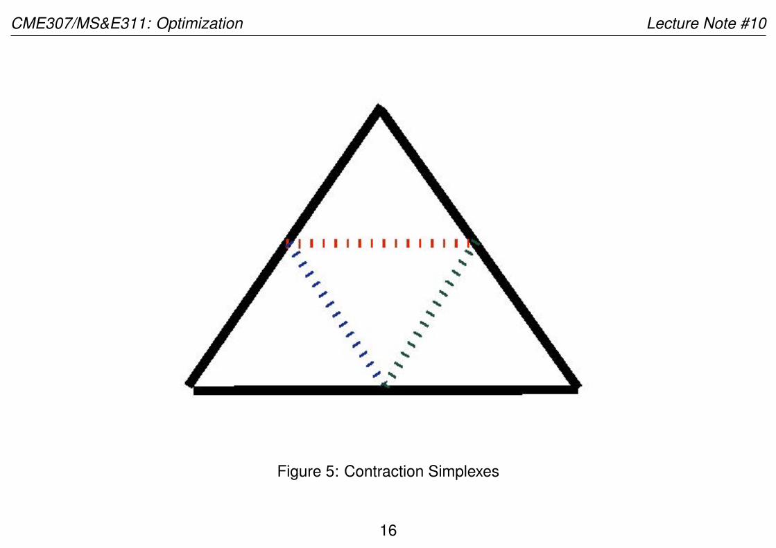
(3) Contraction: Compute the d+ 1 middle-face points and subdivide the simplex into smaller d+ 1

simplexes, keep the simplex with the lowest sum of the d+ 1 function values, and go to Step 1.

This method can be also implemented with exhausted enumeration in parallel.

14


Figure 4: Reflection Simplexes

15


Figure 5: Contraction Simplexes

16


First-Order Algorithm: the Steepest Descent Method (SDM)

Let f be a differentiable function and assume we can compute gradient (column) vector∇f . We want to

solve the unconstrained minimization problem

minx∈Rn

f(x).

In the absence of further information, we seek a first-order KKT or stationary point of f , that is, a point x∗

at which∇f(x∗) = 0. Here we choose direction vector dk = −∇f(xk) as the search direction at xk,

which is the direction of steepest descent.

The number αk ≥ 0, called step-size, is chosen “appropriately” as

αk ∈ arg minf(xk − α∇f(xk)).

Then the new iterate is defined as xk+1 = xk − αk∇f(xk).

In some implementations, step-size αk is fixed through out the process – independent of iteration count k

17


SDM Example: Unconstrained Quadratic Optimization

Let f(x) = 12x

TQx+ cTx where Q ∈ Rn×n is symmetric and positive definite. This implies that the

eigenvalues of Q are all positive. The unique minimum x∗ of f(x) exists and is given by the solution of

the system of linear equations

∇f(x)T = Qx+ c = 0,

or equivalently

Qx = −c.

The iterative scheme becomes, from dk = −(Qxk + c),

xk+1 = xk + αkdk = xk − αk(Qxk + c).

To compute the step size, αk, we consider

f(xk + αdk)

= cT (xk + αdk) + 12 (x

k + αdk)TQ(xk + αdk)

= cTxk + αcTdk + 12 (x

k)TQxk + α(xk)TQdk + 12α

2(dk)TQdk

18


which is a strictly convex quadratic function of α. Its minimizer αk is the unique value of α where the

derivative f ′(xk + αdk) vanishes, i.e., where

cTdk + (xk)TQdk + α(dk)TQdk = 0.

Thus

αk = −cTdk + (xk)TQdk

(dk)TQdk=

∥dk∥2

(dk)TQdk.

The recursion for the method of steepest descent now becomes

xk+1 = xk −(∥dk∥2

(dk)TQdk

)dk.

Therefore, minimize a strictly convex quadratic function is equivalent to solve a system of equation with a

positive definite matrix. The former may be ideal if the system only needs to be solved approximately.

19


Iterate Convergence of the Steepest Descent Method

The following theorem gives some conditions under which the steepest descent method will generate a

sequence of iterates that converge .

Theorem 2 Let f : Rn → R be given. For some given point x0 ∈ Rn, let the level set

X0 = {x ∈ Rn : f(x) ≤ f(x0)}

be bounded. Assume further that f is continuously differentiable on the convex hull of X0. Let {xk} be

the sequence of points generated by the steepest descent method initiated at x0. Then every

accumulation point of {xk} is a stationary point of f .

Proof: Note that the assumptions imply the compactness of X0. Since the iterates will all belong to X0,

the existence of at least one accumulation point of {xk} is guaranteed by the Bolzano-Weierstrass

Theorem. Let x be such an accumulation point, and without losing generality, {xk} converge to x.

Assume∇f(x) = 0. Then there exists a value α > 0 and a δ > 0 such that

f(x− α∇f(x)) + δ = f(x). This means that y := x− α∇f(x) is an interior point of X0 and

f(y) = f(x)− δ.

20


For an arbitrary iterate of the sequence, say xk, the Mean-Value Theorem implies that we can write

f(xk − α∇f(xk)) = f(y) + (∇f(yk))T(xk − α∇f(xk)− y

)where yk lies between xk − α∇f(xk) and y. Then {yk} → y and {∇f(yk)} → ∇f(y) as

{xk} → x. Thus, for sufficiently large k,

f(xk − α∇f(xk)) ≤ f(y) +δ

2= f(x)− δ

2.

Since the sequence {f(xk)} is monotonically decreasing and converges to f(x), hence

f(x) < f(xk+1) = f(xk − αk∇f(xk)) ≤ f(xk − α∇f(xk)) ≤ f(x)− δ

2

which is a contradiction. Hence∇f(x) = 0.

Remark According to this theorem, the steepest descent method initiated at any point of the level set X0

will converge to a stationary point of f , which property is called global convergence.

This proof can be viewed as a special form of Theorem 1: the SDM algorithm mapping is closed and the

objective function is strictly decreasing.

21


Convergence Rate of the SDM for Convex QP

The convergence rate of the steepest descent method applied to convex quadratic functions is known to

be linear. Suppose Q is a symmetric positive definite matrix of order n and let its eigenvalues be

0 < λ1 ≤ · · · ≤ λn. Obviously, the global minimizer of the quadratic form f(x) = 12x

TQx is at the

origin.

It can be shown that when the steepest descent method is started from any nonzero point x0 ∈ Rn, there

will exist constants c1 and c2 such that (page 235, L&Y)

0 < c1 ≤f(xk+1)

f(xk)≤ c2 ≤

(λn − λ1

λn + λ1

)2

< 1, k = 0, 1, . . . .

Intuitively, the slow rate of convergence of the steepest descent method can be attributed the fact that the

successive search directions are perpendicular.

Consider an arbitrary iterate xk. At this point we have the search direction dk = −∇f(xk). To find the

next iterate xk+1 we minimize f(xk − α∇f(xk)) with respect to α ≥ 0. At the minimum αk, the

derivative of this function will equal zero. Thus, we obtain∇f(xk+1)T∇f(xk) = 0.

22


The Barzilai and Borwein Method

There is a steepest descent method (Barzilai and Borwein 88) that chooses the step-size as follows:

∆kx = xk − xk−1 and ∆k

g = ∇f(xk)−∇f(xk−1), (1)

αk =(∆k

x)T∆k

g

(∆kg)

T∆kg

or αk =(∆k

x)T∆k

x

(∆kx)

T∆kg

,

Then

xk+1 = xk − αk∇f(xk). (2)

For convex quadratic minimization with Hessian Q, ∆kg = Q∆k

x, the two step size formula become

αk =(∆k

x)TQ∆k

x

(∆kx)

TQ2∆kx

or αk =(∆k

x)T∆k

x

(∆kx)

TQ∆kx

and it is between the reciprocals of the largest and smallest non-zero eigenvalues of Q (Rayleigh

quotient).

23


An Explanation why the BB Method Works

For convex quadratic minimization, let the distinct nonzero eigenvalues of Hessian Q be λ1, λ2, ..., λK ;

and let the step size in the SDM be αk = 1λk

, k = 1, ...,K . Then, the SDM terminates in K iterations

from any starting point x0.

In the BB method, αk minimizes

∥∆kx − α∆k

g∥ = ∥∆kx − αQ∆k

x∥.

If the error becomes 0 plus ∥∆kx∥ = 0, 1

αk will be a nonzero eigenvalue of Q – this is learning via

Rayleigh quotient.

On the other hand, many questions remain open for the BB method.

24


Step-Size of the SDM for Minimizing Lipschitz Functions

Let f(x) be differentiable every where and satisfy the (first-order) β-Lipschitz condition, that is, for any

two points x and y

∥∇f(x)−∇f(y)∥ ≤ β∥x− y∥ (3)

for a positive real constant β. Then, we have

Lemma 1 Let f be a β-Lipschitz function. Then for any two points x and y

f(x)− f(y)−∇f(y)T (x− y) ≤ β

2∥x− y∥2. (4)

At the kth step of SDM, we have

f(x)− f(xk) ≤ ∇f(xk)T (x− xk) +β

2∥x− xk∥2.

The left hand strict convex quadratic function of x establishes a upper bound on the objective reduction.

25


Let us minimize the quadratic function

xk+1 = argminx∇f(xk)T (x− xk) +

β

2∥x− xk∥2,

and let the minimizer be the next iterate. Then it has a close form:

xk+1 = xk − 1

β∇f(xk)

which is the SDM with the fixed step-size 1β . Then

f(xk+1)− f(xk) ≤ − 1

2β∥∇f(xk)∥2, or f(xk)− f(xk+1) ≥ 1

2β∥∇f(xk)∥2.

Then, after K(≥ 1) steps, we must have

f(x0)− f(xK) ≥ 1

2β

K−1∑k=0

∥∇f(xk)∥2. (5)

Theorem 3 (Error Convergence Estimate Theorem) Let the objective function p∗ = inf f(x) be finite

and let us stop the SDM as soon as ∥∇f(xk)∥ ≤ ϵ for a given tolerance ϵ ∈ (0 1). Then the SDM

26


terminates in 2β(f(x0)−p∗)ϵ2 steps.

Proof: From (5), after K = 2β(f(x0)−p∗)ϵ2 steps

f(x0)− p∗ ≥ f(x0)− f(xK) ≥ 1

2β

K−1∑k=0

∥∇f(xk)∥2.

If ∥∇f(xk)∥ > ϵ for all k = 0, ...,K − 1, then we have

f(x0)− p∗ >K

2βϵ2 ≥ f(x0)− p∗

which is a contradiction.

Corollary 1 If a minimizer x∗ of f is attainable, then the SDM terminates in β2∥x0−x∗∥2

ϵ2 steps.

The proof is based on Lemma 1 with x = x0 and y = x∗ and noting∇f(y) = ∇f(x∗) = 0:

f(x0)− p∗ = f(x0)− f(x∗) ≤ β

2∥x0 − x∗∥2.

27


Forward and Backward Tracking Step-Size Method

In most real applications, the Lipschitz constant β is unknown. Furthermore, we like to use the smallest

localized Lipschitz constant βk at iteration k such that

f(xk + αdk)− f(xk)−∇f(xk)T (αdk) ≤ βk

2∥αdk∥2,

where dk = −∇f(xk), to decide the step-size α = 1βk .

Consider the following step-size strategy: stat at a good step-size guess α > 0:

(1): If α ≤ 2(f(xk)−f(xk+αdk))∥dk∥2 then doubling the step-size: α← 2α, stop as soon as the inequality is

reversed and select the latest α with α ≤ 2(f(xk)−f(xk+αdk))∥dk∥2 ;

(2): Otherwise halving the step-size: α← α/2; stop as soon as α ≤ 2(f(xk)−f(xk+αdk))∥dk∥2 and return it.

Prove that the selected step-size1

2βk≤ α ≤ 1

βk.

28

Zero-Order and First-Order Optimization Algorithms I · One-Variable Optimization: Golden Section...

Documents

Transcript of Zero-Order and First-Order Optimization Algorithms I · One-Variable Optimization: Golden Section...