Your use of the JSTOR archive indicates your acceptance of...
39
Wiley and Royal Statistical Society are collaborating with JSTOR to digitize, preserve and extend access to Journal of the Royal Statistical Society. Series A (General). http://www.jstor.org Tests of Significance for 2 × 2 Contingency Tables Author(s): F. Yates Source: Journal of the Royal Statistical Society. Series A (General), Vol. 147, No. 3 (1984), pp. 426-463 Published by: for the Wiley Royal Statistical Society Stable URL: http://www.jstor.org/stable/2981577 Accessed: 26-08-2014 23:40 UTC Your use of the JSTOR archive indicates your acceptance of the Terms & Conditions of Use, available at http://www.jstor.org/page/info/about/policies/terms.jsp JSTOR is a not-for-profit service that helps scholars, researchers, and students discover, use, and build upon a wide range of content in a trusted digital archive. We use information technology and tools to increase productivity and facilitate new forms of scholarship. For more information about JSTOR, please contact [email protected]. This content downloaded from 137.151.37.0 on Tue, 26 Aug 2014 23:40:14 UTC All use subject to JSTOR Terms and Conditions
Transcript of Your use of the JSTOR archive indicates your acceptance of...

Wiley and Royal Statistical Society are collaborating with JSTOR to digitize, preserve and extend access to Journal of theRoyal Statistical Society. Series A (General).
http://www.jstor.org
Tests of Significance for 2 × 2 Contingency Tables Author(s): F. Yates Source: Journal of the Royal Statistical Society. Series A (General), Vol. 147, No. 3 (1984), pp.
426-463Published by: for the Wiley Royal Statistical SocietyStable URL: http://www.jstor.org/stable/2981577Accessed: 26-08-2014 23:40 UTC
Your use of the JSTOR archive indicates your acceptance of the Terms & Conditions of Use, available at http://www.jstor.org/page/info/about/policies/terms.jsp
JSTOR is a not-for-profit service that helps scholars, researchers, and students discover, use, and build upon a wide range of contentin a trusted digital archive. We use information technology and tools to increase productivity and facilitate new forms of scholarship.For more information about JSTOR, please contact [email protected].
This content downloaded from 137.151.37.0 on Tue, 26 Aug 2014 23:40:14 UTCAll use subject to JSTOR Terms and Conditions

J. R. Statist. Soc. A (1984), 147,Part 3, pp. 426-463
Tests of Significance for 2 X 2 Contingency Tables
By F. YATES Rothamsted Experimental Station
[Read before the Royal Statistical Society on Wednesday, March 21st, 1984, the President Professor P. Armitage in the Chair]
SUMMARY Fisher's exact test, and the approximation to it by the continuity-corrected X2 test, have repeatedly been attacked over the past 40 years, recently with the support of extensive computer exercises. The present paper argues, on commonsense grounds, supported by simple examples, that these attacks are misconceived, and are mainly due to uncritical acceptance of the Neyman-Pearson approach to tests of significance, the use of nominal levels, and refusal to accept the arguments for conditioning on the margins.
Two-sided tests have also added to the confusion; it is argued that the best definition of a two-sided probability is twice the observed one-tail probability.
Keywords: ANCILLARY STATISTICS; BINOMIAL PROBABILITIES; CONDITIONING; CONSERVATIVE TEST; CONTINGENCY TABLES; CONTINGENCY TEST; CONTINUITY CORRECTION; FISHER'S EXACT TEST; GOODNESS OF FIT; NEYMAN-PEARSON THEORY; ONE-TAIL PROBABILITIES; QUALITY CONTROL; SIGNIFICANCE TESTS; TWO-SIDED TESTS; YATES'S CORRECTION
1. INTRODUCTION Tests of significance for evidence of association from data in 2 x 2 contingency tables have long been a matter of dispute. Ever since its introduction the legitimacy of Fisher's exact test has been under attack, mainly on the ground that it is too"conservative", i.e. that it gives fewer significant results than are justified by the evidence provided by the data, except for tables both margins of which are determined in advance.
These disputes are attributable to the fact that Neyman and Pearson, in the development of their theory of tests of significance, took it as axiomatic (or as Pearson preferred to call it, as a practical requirement) that the level of significance must be equal to the frequency with which the hypothesis is rejected in repeated sampling of any fixed population allowed by hypothesis. That this was indeed the basis of the earliest ideas on tests of significance is unquestionably true. These had their genesis in the concept of probability associated with games of chance, later extended, by the normal theory of errors, to errors in estimates based on continuous variables. The latter, of course, requires knowledge of the standard deviation or its estimation from the available data. It was Gosset's introduction of the t-test, which made due allowance for errors of estimation of a from sparse data, that led to Fisher's recognition that conditioning on ancillary statistics (i.e. statistics that provide information on the accuracy of the estimated quantity but do not themselves contain any information on this quantity) is a fundamental and valuable extension of the theory of tests of significance.
The t-test was acceptable to the Neyman-Pearson school because it did not transgress the frequency requirements of repeated sampling. The marginal totals of a contingency table have a function similar to s2 in that they provide no information, additional to that provided by the
Present address: Rothamsted Experimental Station, Harpenden, Herts ALS 2JQ.
? 1984 Royal Statistical Society 0035-9238/84/147426 $2.00
This content downloaded from 137.151.37.0 on Tue, 26 Aug 2014 23:40:14 UTCAll use subject to JSTOR Terms and Conditions

1984] Tests of Significance 427
body of the table, on lack of proportionality, but do provide information on the accuracy of estimates of association. However, like the Behrens-Fisher test, though for somewhat different reasons, the frequency requirements of repeated sampling are not satisfied.
The frequency property, when it holds, is undoubtedly an easy way of explaining what is meant by tests of significance; indeed Fisher lent support to this mode of explanation in much of his early writing. Any numerate person, for example, is aware of the probabilities associated with simple games of chance, such as tossing a coin or spinning a roulette wheel, and anyone who has any experience of errors of measurement can fully appreciate the implications of the normal theory of errors. Because the frequency requirement is not violated he is not likely to dispute the t-test, though he may feel some unease if the number of degrees of freedom for error is very small. He is much more disposed, however, to doubt the need for conditioning in tests of 2 x 2 contingency tables, particularly as he is often anxious to use the results of such tests to prove that some association is indicated, and is consequently the more ready to believe that the exact test is "conservative".
It is this mistaken belief that has prompted me to write this paper. The points at issue are illustrated by simple examples, mostly based on very small numbers, partly because of ease of presentation, but also because it is here that the contradictions between the two theories are most evident. As the size of a sample is increased the discrepancies between the different approaches are steadily reduced, though it should be remembered that these discrepancies are primarily dependent on the smallest expectation of any cell, not on the total number of observations in the table.
In addition to conditioning, the consequences of using nominal levels of significance, such as 5 and 1 per cent, are also discussed; this practice is a further defect of the Neyman-Pearson theory which undoubtedly adds to the general confusion. Two-sided tests are a further source of disagreement.
Fisher's exact test is closely related to the x2 test, which is itself a conditional test; indeed the continuity-corrected x2 gives close approximations to the exact test, except for tables with very small expectations. A brief history of the development of these tests, and some comments on some recent papers criticising the exact test, are included in the present paper.
A more mathematical matter that has entered into the disputes is the question of whether the marginal values of a table really contain no additional information on the existence of association, and therefore qualify as ancillary statistics. This is a more technical issue which is relegated to a short appendix.
2. NOTATION In what follows the numbers in a 2 x 2 table are represented by the symbols of Table 1, where,
in general, ml < m2, n1 <n2 and q1 = 1 -Pl, etc. With given margins, a, which is then the cell
TABLE 1 Notation
B1 B2 Total
A1 a b n1 P1 = aln1 A2 c d n2 P2 c/n2
Total ml m2 N p =m,IN
with the smallest expectation, can assume integral values of 0 to m1 if m1 ? n1, or 0 to n1 if m1 > n1 . The expectation e of a, when there is no association, equals m1 n1 /N. In some contexts Pi and P2 can be regarded as estimates of binomial probabilities Pi and P2 - If Pl = P2 = p say, a combined estimate of p is given by p.
To save space numerical values for particular tables are given in the text in the form (a, b; c, d).
This content downloaded from 137.151.37.0 on Tue, 26 Aug 2014 23:40:14 UTCAll use subject to JSTOR Terms and Conditions

428 YATES [Part 3,
Occasionally the form {m1, mi2; n1, n2; N} is used for marginal values. In the text, also, the word "table" is used in two senses, (i) a table with particular numerical values for a, b, c, d, (ii) the family of tables, ml + 1 or nI + 1 in number, which contain values of a, b, c, d conform- ing to the given numerical marginal totals. It will be obvious from the context which sense is implied.
If mlI ? n1 and p' n 1/N = e/m1 the distribution of a will tend to the binomial distribution (p' +q')ml as N- co with ml1 and e fixed; and similarly, with ml1 and n1 interchanged, if ml1 >n1.
3. EARLY HISTORY
In 1900 Karl Pearson introduced the x2 test for goodness of fit. The test has proved to be of great utility in many contexts, but unfortunately Pearson did not recognize that in addition to deducting one degree of freedom for the number in the sample an additional degree of free- dom must be deducted for each additional parameter estimated from the data. In testing for association in contingency tables the expectations of the cell values are estimated from the marginal totals, and the number of degrees of freedom for an r x s table is therefore (r - 1) (s - 1), not rs - 1. This error is particularly serious in 2 x 2 tables, for which x2 with one degree of free- dom must be used, not three degrees of freedom as Pearson thought.
Udny Yule was also very concerned with contingency tables, and introduced a test for association in 2 x 2 tables in his textbook, Introduction to the Theory of Statistics, first published in 191 1, using the large-sample estimate <(pq/n) for the standard error of a proportion p. This gives an estimate of the standard error of the observed difference, Pl -P2, of the two probabilities, of
p( q) P2q2 n, n2
He also noted that if there is no difference Pi and P2 can both be replaced by their combined estimate p = m1 /N. With this combined estimate Yule's test is equivalent to Pearson's x2 test with one degree of freedom. The most convenient formula for this is
(ad - bc)2 N (1)
ml M2 n1 n2
Yule did not mention the x2 test in his textbook, but he evidently soon became aware of the discrepancy between his test and the x2 test with three degrees of freedom, as he drew attention to it in Greenwood and Yule (1915), and shortly afterwards constructed 350 2 x 2 tables and 100 4 x 4 tables by mechanical devices designed to give independent distributions, and compared the X2 distributions so obtained with those given by theory, but did not immediately publish his results.
The next event of importance was the publication by R. A. Fisher of his 1922 paper, in which he drew attention to Pearson's error. Although Yule was not fully satisfied with Fisher's proof he then simultaneously published the results of his sampling investigation, which, as was to be expected, confirmed Fisher's results. Pearson, as was his wont, did not immediately admit to any error, and a considerable controversy arose, but the correctness of Fisher's conclusions ultimately came to be generally accepted.
The x2 test is of course approximate and will not hold exactly when the expectations of the separate cells of a distribution or contingency table are small. In Statistical Methods for Research Workers (1925) Fisher advanced a rule of thumb that the expected number in any one cell should not be less than 5. This rule may in fact be adequate, indeed conservative, for tests involving more than one degree of freedom. It is more suspect for tests involving only a single degree of freedom. Such tests are special in that there are two separate tails, which should be kept distinct. A x2 test with 1 df is in fact equivalent, if the appropriate sign is attached to '/x2, to a test of a normal deviate with unit standard deviation.
This content downloaded from 137.151.37.0 on Tue, 26 Aug 2014 23:40:14 UTCAll use subject to JSTOR Terms and Conditions

1984] Tests of Significance 429
If the exact distribution relevant to any particular problem is known the accuracy of the x2 test (or any other approximate method) can be investigated by comparing its performance with that given by the exact distribution over a range of typical examples. In 1933 I became interested in such an investigation. The exact form of a binomial distribution with given p was of course well known, but not that of a 2 x 2 table with given marginal totals. This was suggested to me by Fisher, and depends on the restriction that only sets of values conforming to both pairs of observed marginal totals are included in evaluating the probabilities, a restriction which is in fact also implicit in the x2 test, as the expectations of the cell values are calculated from the marginal totals. Although then unpublished, the exact form must have been known to Fisher for some years, as is indicated by a cryptic passage in an earlier paper (Fisher, 1926): "an exact discussion would show that [for tables with 35 entries] the average value of x2 should exceed unity by one part in 34".
The results of this investigation, reported in my 1934 paper, showed that the approximations given by x2 to both binomial and 2 x 2 exact probabilities, particularly when the parent distributions are approximately symmetrical, are greatly improved by deducting 1/2 from the observed deviations from expectations when calculating x2. This I termed the continuity correction. Formula (1) above then becomes
= (lad - bc -N)2 N ml m2 n1 n2
If, however, the parent distribution, as for example a binomial distribution with p differing greatly from 0.5, is markedly asymmetrical, the one-tail probability given by Xc, the square root of X2 corrected for continuity, will necessarily deviate somewhat from the true probability, because the normal distribution to which it is referred is symmetrical. I therefore produced a small table, covering 2 x 2 tables and binomial and Poisson distributions, of the Xc values for the 2.5 per cent and 0.5 per cent significance levels, corresponding to the 1.96 and 2.58 values for the normal distribution. This was later included in Statistical Tables (Fisher and Yates, 1938). Fisher also added sections on the continuity correction and the exact test to the 5th edition (1934) of Statistical Methods for Research Workers, Sections 21.01, 21.02. He also (1935) stated his reason for believing that the exact test should always be used, whether or not the margins are determined in advance.
One might have thought that this would settle the matter, particularly as the X2 test had come to be recognized as the appropriate test when the expectations in all four cells of the table are reasonably large. However, in 1945 Barnard put forward a test which he claimed was more powerful than Fisher's exact test (Barnard, 1945). Taking the table to be generated by samples of n1 and n2 from two binomial distributions with probabilities Pi and P2, he argued that if PI = P2 = p and n1 = n2= 3, for example, the probability of getting the table (3,0; 0,3) is p3 q3 e which has the value 1/64 when p = 0.5, and is less than this for all other values of p, as opposed to a probability of 1/20 if both margins are regarded as fixed.
At first sight, Barnard's argument seems to make good sense. It is certainly true that if we take repeated pairs of samples from two binomials each with p = 0.5, 1 in 64 pairs on the average will give the table (3,0; 0,3). This, however, is equivalent to taking a sample of 6 from a single binomial, and dividing it at random into two triplets. From the binomial distribution (1/2 + 1/2)6 the probability of getting values of 3,3 in the ml, m2 margin is 20/64. Thus the combined probability of getting the table (3,0; 0,3) is 20/64 x 1/20 = 1/64. The crucial question, therefore, is whether the factor 20/64 should be included in the calculation of the significance probability.
Barnard later (1947) elaborated his proposal into what he termed the CSM test. A somewhat similar proposal had also been made by E. B. Wilson (1941). Both proposals were soon abandoned, however, and Fisher was able to write in his discussion of the problem in Statistical Methods and Scientific Inference (1956):
This content downloaded from 137.151.37.0 on Tue, 26 Aug 2014 23:40:14 UTCAll use subject to JSTOR Terms and Conditions

430 YATES [Part 3,
"Professor Barnard has since then frankly avowed [(1949)] that further reflection has led him to the same conclusion [that only samples conforming to the observed marginal totals rank for inclusion] as Yates and Fisher, as indeed Wilson with equal generosity had done earlier." That this conclusion is still not accepted in many quarters, however, is very evident from
numerous recent publications. The simple numerical examples in the following sections will, it is hoped, throw further light on the points at issue, and illustrate the ways in which tests of significance, correctly applied, can be of help in the interpretation of 2 x 2 data.
4. COMPARATIVE TRIALS If, say, we wish to test whether inoculation with a new serum reduces the risk of contracting
some infectious disease, a group of N individuals may be chosen for the test and n1 of them selected at random for inoculation, leaving the remainder n2 uninoculated. This determines the nl, n2 margin. Moreover if none of the N individuals were inoculated a given number ml (unknown to the experimenter) would be fated to contract the disease. If the inoculation has no effect this will not be changed by the experiment. Subject to this condition, therefore, the ml, m2 margin is also determined. The statistical problem, if there is an apparent beneficial effect of inoculation, is the evaluation of the probability that the observed or a greater apparent effect can be attributed to chance causes resulting from the random assignment of the inoculation treatment; and conversely if there is an apparent deleterious effect the evaluation of the probability of getting a negative effect of this or greater magnitude by chance.
Given the marginal values, and random selection for inoculation, the probability of the occurrence of any particular set of cell values (a, b; c, d) when inoculation has no effect can be shown by combinatorial analysis to be
ml! m2! nl! n2!
a b! c! d!N! This gives Fisher's exact distribution. If mln In there will be ml + 1 terms, with values of a from 0 to ml; if ml >nl there will be n1 + 1 terms. If ao is the observed value, summation of the probabilities from the lower or upper tail gives the probability of getting a value of a < or > ao. This provides an exact test of the signiflcance of an apparent association. With given values of n, and n2 there will be a set of such distributions, N + 1 in number, the relevant distribution being determined by the observed values of ml, m2. The figures in brackets in Table 2 show the 11 distributions obtained when nI = n2= 5.
It should be noted that Barnard did not, in his 1947 paper, discuss comparative trials, but uses the term, misleadingly in my opinion, for samples from two binomials.
5. SAMPLES FROM TWO BINOMIALS In a comparative trial the individuals included are not necessarily chosen at random from a
defined larger population-they may merely be selected as suitable experimental material. In many 2 x 2 tables, however, the data are in fact, or can be regarded as, samples from two defined large populations, in which case the two lines of the table constitute samples of n1 and n2 from two binomial distributions. If Pi and P2 are the binomial probabilities and there is no association, so that P1 = P2 = p say, a combined estimate p = m1/N from the m1, m2 margin provides a sufficient estimate of p. Conditioning on this estimate, i.e. regarding the ml, M2 margin as "fixed", then gives Fisher's exact distribution. If, however, we do not impose this conditioning, and instead consider all combinations of the possible samples of n1 and n2 that can arise from the two binomial distributions, their associated probabilities, ranked in order of the values of P I - P2, or in some other plausible manner, will provide a basis for an alternative test of whether Pi differs significantly from P2. This was the basis of Barnard's "more powerful" CSM test.
The following specific example may help to clarify thinking on this matter. Table 2 sets out
This content downloaded from 137.151.37.0 on Tue, 26 Aug 2014 23:40:14 UTCAll use subject to JSTOR Terms and Conditions

1984] Tests of Significance 431
t :t H O t F~~0 In in uz4 -- 0 0o E 4 O H t ^ O ~~~~t O~ 0
S~~~~~~~~~~nR 0 m00 0 O %D 000 I
I I o t. t. ?o I It- t a o t m?^ o^ oOoF om^ mt o n E~~~R
4 CJ t > uz n O r uz n a, n a% <
4i~ I n
0. o 0
o O |0 |n It
X 1 n oOO oo oo ooOo > .: > - tn
X~~~~ ~~~ S- 00 on 1- in ? >4
t N:m~~~~~~~~~t
SL i I I I i + ~~~~+ + + +
This content downloaded from 137.151.37.0 on Tue, 26 Aug 2014 23:40:14 UTCAll use subject to JSTOR Terms and Conditions

432 YATES [Part 3,
the relative frequencies (probabilities x 1024) of the 36 possible outcomes with n, - n2 = 5 and p = 1/2. In the table the outcomes are classified by the differences between Pi and P2 and by the values of the marginal totals ml, M2-
The table enables the probability of obtaining samples with any given characteristics, with or without conditioning onw the ml, m2 margin, to be calculated. For samples in which p, -P2 > 0.6, for example, the probability without conditioning is (10 + 25 + 10 + 5 + 5 + 1)/ 1024 = 0.055, or directly by the marginal totals (45 + 10 + 1)/1024. These marginal totals are in fact 1024 times the relative frequencies, shown in the right-hand margin, of the binomial (1/2 + 1/2)10. Thus if we were betting on P1 - P2 > 0.6 without knowledge of the ml, m2 margin the fair betting odds would be (1024-56): 56 or 17: 1 approximately.
If, however, we were informed, by the person taking the samples, of the marginal totals mlI, m2 for each particular sample, the conditional probabilities (shown in brackets) would enable us to make much more discriminating bets. We would, if we were wise, only bet when marginal totals of 5, 5, 7, 3 or 3, 7 occurred. For 5, 5 the probability of a successful bet is (25 + 1)/252 = 0.103, and for 7, 3 and 3, 7 is 10/120 = 0.083. For margins 6, 4 and 4, 6 the probability of success is only 5/210 = 0.024 and for the remainder is zero.
Gambling of this type can easily be performed with two packs of cards. If, after shuffling, 5 cards are dealt from each pack, and if the numbers of red cards are at issue, this is equivalent, apart from the fact that the packs constitute finite populations, to independent samples of 5 from two binomial distributions each with p = 1/2. If the sample cards are laid on the table face downwards all we can say about the probability that there are three, four, or five more red cards in the sample from pack A than in that from pack B is that its overall value is 0.055, and this should govern the betting. If, however, the 10 sample cards are shuffled and then displayed face upwards, the total numbers of reds and blacks are immediately apparent, although we still do not know to which pack each individual card belongs. If one of the opponents is aware of the value of this information, and takes cognisance of it, while the other pins his faith on the overall probability, the latter is clearly likely to find himself considerably out of pocket.
To obtain more precise probabilities account must be taken of the fact that the samples are ftom finite populations of 52 cards. In such samples the probabilities of getting 0,1, .. ., 5 red cards are approximately (1, 6, 13, 13, 6, 1)/40, instead of the binomial probabilities of (1, 5, 10, 10, 5, 1)/32. Substitution of these new values in the diagonal margins of the square of values of Table 2, with corresponding adjustments to the values in the body of the square, gives an overall probability of 0.047 of an excess of 3 or more red cards in pack A, i.e. fair betting odds of 20:1 instead of 17: 1; if the margins are revealed and bets are placed only for margins 5, 5, 7, 3, 3, 7 the average gain per bet at odds of 20: 1 will be 70 per cent of the stake, compared with 68 per cent at odds of 17: 1 for true binomial sampling.
The conditional probabilities differ somewlhat from those given by the exact distribution for random sampling from two infinite populations with the same p. The last two values for the 5, 5 margin, for example, are 0.087 and 0.0024 instead of 0.099 and 0.0040. This may at first sight seem surprising, but a little consideration will show that generation of a table in this manner from two finite populations is not equivalent to the random allocation of treatments adopted for a comparative trial.
The frequencies in Table 2 relate to p = 1/2. Those for p = 1/4, for example, can be obtained by multiplying the values in the successive columns by 1, 3, 9, 27 .... This gives a total over the whole table of 410 and an overall probability that P2 -Pi p 0.6 of 0.031 instead of 0.055. The conditional probabilities, based on knowledge of ml, m2, are, however, unaltered. The lower overall probability is due to differences in the frequency of occurrence of the different values of ml, M2; 3,7 for example,will occur 81 times as frequently as 7,3, and the five central ml, m2, which are the only ones in which P2 -P1 can possibly be > 0.6, will only occur in 55 per cent of all samples instead of 89 per cent.
From the above it will be seen that knowledge of the ml, m2 margin merely provides a measure of the sensitivity of the observed sample to departures from the null hypothesis. Although some-
This content downloaded from 137.151.37.0 on Tue, 26 Aug 2014 23:40:14 UTCAll use subject to JSTOR Terms and Conditions

19841 Tests of Signifcance 433
times disputed (see the Appendix), it seems to me obvious, as it did to Fisher, that the margins of a 2 x 2 table, however generated, provide virtually no information on the existence of association. In samples from two binomials, for example, absence of association implies that Pi = P2: if n = n2, differences between Pi and P2 of a given magnitude but opposite signs occur with equal frequency, as is shown by Table 2; this does not hold if n1 #: n2, but the mean value of p1 - P2 for given mi, M2 is still zero. ml, M2 are therefore ancillary statistics, in the Fisherian sense, and define a "recognizable subset" (Statistical Methods and Scientific Inference, pp. 32, 109). It is the probabilities of occurrence in the relevant subset that provide the correct basis for tests of significance. In other words, we must condition on the margins, whatever the origin of the table. Whether no, one or two margins are "fixed" in advance is irrelevant.
It is still sometimes represented (e.g. Kempthorne, 1979; Upton, 1982) that although conditioning on the margins is justified by the necessity for randomization in comparative trials such as the inoculation experiment described in Section 4, this does not apply to samples from two binomials, for which "more powerful" unconditional tests are available. This line of reasoning is fallacious. If, for example, the subjects for the inoculation trial of Section 4 had been obtained by selecting a random sample of 10 individuals from some larger population and then assigning these individuals at random to the inoculated-non-inoculated groups, we might alternatively have combined the two steps by taking samples of 5 individuals each from the population, which is notionally equivalent to dividing the population into two populations and taking a sample from each. The difference between a trial of this, type and one on a haphazard collection of individuals is that (subject to the qualification that any extensive use of inoculation is likely to reduce the subsequent risk rate) any results that emerge relate to all the individuals in the parent population. Tests of significance are unaffected.
If the differences between two separate populations are being investigated the notional division above has a real existence, and the actual differences replace those produced by the imposed treatments. Statistically, therefore, the two situations are equivalent and the same tests of signifi'cance must be used.
With discontinuous data, subdivision of the possible outcomes into subsets does, of course, inevitably reduce the significance level of the more extreme outcomes, because only the proba- bilities of outcomes belonging to the relevant subset will enter into the calculation of the significance. It is this fact, I think, and the urge to find "more powerful" tests, regardless of their relevance, that gives rise to the fatal attraction of unconditional tests for discontinuous data. In continuous data conditional tests have long been accepted without question, at least provided that a significance level P is attained with frequency P in repeated sampling. In testing for significance of a linear regression, for examnple, the formula V(b) = J2/S(x - x~)2 is used if the variance u2 of y is known, or indeed if it is estimated from the observations, whether the values of x are preassigned or random, provided only that any unknown parameters in the distribution of x are unrelated to the parameters of interest.
6. CHANGES IN MARGINAL TOTALS DUE TO TREATMENT EFFECTS Part of the reluctance to accept the fact that for the purpose of the test of significance in a
comparative trial the M1, M2 margin must be taken as known, possibly stems from the knowledge that if the treatment does have an effect ml and M2 wil certainly be changed.
Consider a specific example. Suppose we are confident that an inoculation treatment provides sure protection against a certain disease and wish to demonstrate this by doing a trial on 10 sub- jects, 5 of which are to be inoculated, the other 5 not. The success of such a demonstration depends critically on the number of subjects "at risk", i.e. those who will contract the disease if uninoculated. Table 3 shows the distribution of significant and non-significant results for differing numbers at risk when the inoculation is completely successful. The table is constructed as follows. If all 10 subjects are at risk a table with the values (0, 5; 5,0) will always be obtained, giving from Table 2 a significance level of 0.004. If only 8 are at risk then before inoculation mI, M2 will have the values 8, 2. The chances of obtaining initial cell values for inoculated, unin-
This content downloaded from 137.151.37.0 on Tue, 26 Aug 2014 23:40:14 UTCAll use subject to JSTOR Terms and Conditions

434 YATES [Part 3,
TABLE 3 Percentages of significant results in trials with 10 subjects when inoculation
gives certain protection against infection
Number at risk* Significance
c,d level (P) 10 9 8 7 6 5 4 3 <3
5,0 0.004 100 50 22 8 2 0.4 - - - 4,1 0.024 - 50 56 42 24 10 2 - - 3, 2 0.083 - - 22 42 48 40 24 8 - 2, 3 etc. >0.222 - - - 8 26 40 74 92 100
* Those who will become infected if not inoculated.
oculated, of (3, 2; 5, 0), (4, 1; 4, 1), (5, 0; 3, 2) are consequently, from Table 2, 0.222, 0.556, 0.222. On completion of the experiment the first (inoculated) row of each of these tables will become 0, 5, giving significance levels, again from Table 2, of 0.004, 0.024, 0.083 respectively.
This example illustrates another point. If all 10 subjects are at risk, and one of those inoculated contracts the disease, the table (1, 4; 5, 0) will be obtained. This has the same significance level, 0.024, as (0, 5; 4, 1), the second of the two outcomes above when 9 subjects are at risk, but the interpretation is different: here the claim that the inoculation is always successful is definitely disproved, whereas the latter result merely indicates that at least one of the subjects was not at risk.
A statistician reporting on a 2 x 2 table, therefore, should not regard determination of a formal significance level as his sole duty. The two extreme outcomes in an inoculation trial, (0, 5; 0, 5) and (5, 0; 5, 0), for example, both give P = 1.0; the former merely indicates that all or most of the test subjects were not at risk, and that further trials should be made on more suitable material; the latter that inoculation is clearly not very effective.
The latter result does not, of course, imply that inoculation provides no protection. Upper limits to Pi at various significance levels (P) can be obtained from the limits of expectation for the p of a binomial distribution; for a = 0, n1 = 5 and P- 0.1, 0.025, 0.005 the upper limits for p are 0.37, 0.52, 0.65 (Statistical Tables, Table VIII.1).
7. EFFECT OF INCREASING THE NUMBER OF CONTROLS Many 2 x 2 comparative trials consist of the comparison of a new treatment against some
standard or no treatment. In such cases additional controls can often be included at little extra cost. If so there will be a useful gain in the sensitivity of significance tests and in the accuracy of estimates of the difference between Pi and P2-
As an example consider the effect on tests of significance of doubling the number of unin- oculated subjects in the test of the last section. We now have n1 = 5, n2 = 10, giving 66 possible outcomes of the test. The percentages of significant results with varying numbers of subjects at risk are shown in Table 4. These are calculated in the same manner as those of Table 3. To
TABLE 4 Effect of increasing the number of controls: percentages of significant results in' trials
with 5 inoculated and 10 uninoculated subjects when inoculation gives certain protection
Number at risk Significance
c level (P) > 12 12 11 10 9 8 7 6 5 <5
10, 9, 8 < 0.01 100 74 41 17 5 1 - - - - 7 0.019 - 26 44 40 24 9 2 - - - 6 0.042 - - 15 35 42 33 16 4 - - 5 0.084 - - - 8 25 39 39 25 8 -
< 5 > 0.154 - - - - 4 18 43 71 92 100
This content downloaded from 137.151.37.0 on Tue, 26 Aug 2014 23:40:14 UTCAll use subject to JSTOR Terms and Conditions

1984] Tests of Significance 435
facilitate comparison between the two tables some significance levels have been grouped together in Table 4.
As is to be expected the addition of extra controls substantially increases the sensitivity of the test. If 80 per cent of the subjects are at risk, for example, then with additional controls 74 per cent of all tests attain a significance level < 0.01, and the remaining 26 per cent a level < 0.025, whereas without additional controls the corresponding figures are 22 per cent and 56 per cent, the remaining 22 per cent being non-significant.
8. FISHER'S TEA-TASTING EXPERIMENT The example in the last section illustrates the insight that can be gained, when planning experi-
ments on quantal data, by studying the performance of tests of significance under various circumstances, using postulated real effects. A further example which I found intriguing is an experiment described by Fisher in the Design of Experiments. Its object was to test a lady's claim that she could tell, when drinking tea, whether the milk had been poured before or after the tea. As designed by Fisher, the experiment provides a classic and somewhat rare example of the generation of a 2 x 2 table in which both margins are determined in advance.
In this experiment the lady was offered eight cups of tea, and was asked to decide which of these had the milk added first, and which last, having been informed there were in fact four of each kind. Suppose the lady has definite discriminating ability, but is sometimes in doubt as to the correct verdict. If there are no doubtful cases the outcome (4, 0; 0, 4) will result, giving a significance probability of 1/70. Uncertainty on one cup only will give the same result, as it will be assigned to the group with only three cups. The same will happen if there are two uncertainties both belonging to the same group. But if these belong one to each group, there will be a 50 per cent chance of wrong assignment. This will give the outcome (3, 1; 1, 3), and a probability of 17/70 of getting this or a better result. The unbracketed values in the "no rejects" columns of Table 5 summarize these results.
If the lady is not informed in advance that there are four cups of each kind the ml, m2 margin is not determined, and she will consequently no longer be able to make correct assignments with certainty for the 1, 0 and 2, 0 distributions; there is also an additional possible pair of outcomes in the 1, 1 case. These cases are shown in square brackets. They indicate the advantage to the subject of the information on the constitution of what is submitted for test.
If, however, the lady is permitted to declare her uncertainties, and these are omitted from the assessment of significance, we obtain the results shown in the last two columns of Table 5. These generate a nicely graded set of probabilities which give a fairer assessment of the subject's true power of discrimination, not marred by the potential chance failure in the 1, 1 case, but giving due credit to correct clear-cut judgements.
9. NOMINAL LEVELS OF SIGNIFICANCE A contributory cause of confusion that affects discontinuous data is the use of conventional
nominal levels of significance such as 5 and 1 per cent. This was partly engendered by the use of the nominal significance probability for the argument in tables of t and the normal distribution. This did tend to encourage practical workers to think that if an experiment gives a non-significant result at the chosen level not only is the existence of a real effect not established, but that there is in fact no effect. This mode of thought was further encouraged by the mathematical symbolism adopted by the Neyman-Pearson school: Ho: 0 = 0, H1: C $ 0, or the even more absurd, if 0 can be negative, Ho: 0 = 0, H1: 0 > 0.
In quantitative experiments the practice of ornamenting tables by one, two or three stars to denote 5, 1 and 0.1 per cent significance is a convenient way of drawing attention to the more outstanding effects, though this does not obviate the need to report standard errors. With dis- continuous data, however, the use of nominal levels can be seriously misleading. The chance of getting 8 or more heads in 10 tosses of a coin, for example, is 0.055, and that for 9 or more heads is 0.011, as can easily be calculated from the binomial (1/2 + 1/2)10 Here no conditioning (except
This content downloaded from 137.151.37.0 on Tue, 26 Aug 2014 23:40:14 UTCAll use subject to JSTOR Terms and Conditions

436 YATES [Part 3,
It_
4 a oX Q O O-O N
vm~~~o tt F 0
40~~ 0 X_
8 S ~~~~~~~~~t t It It
'E0~ f4
?t~~~~~~~~~~C C; C;^?
I:4
4.k b 000
c t a .^ *e t m
St <O n n^^ 0
* U
U z z ? '-40.=
b $ ta
Q . ; Ps~~ A ~oo o
This content downloaded from 137.151.37.0 on Tue, 26 Aug 2014 23:40:14 UTCAll use subject to JSTOR Terms and Conditions

1984] Tests of Significance 437
on the number in the sample) is involved, but provided the coin is unbiased only 1.1 per cent of all samples on average will be declared significant at a nominal level of 5 per cent. The actual significance probability attained should therefore always be given when reporting on discontinuous data.
Concentration on single-tail nominal levels of 2.5 and 0.5 per cent is a defect in my 1934 paper, which reflects the current thinking of that time. It may be noted, however, that although Fisher was himself in large part responsible for the widespread use of nominal levels, he always gave actual significance levels when discussing discontinuous examples.
10. QUALITY CONTROL Tests based on 2 x 2 tables are sometimes required for quality control. An early example is
provided by Pearson (1947). This was for testing the performance of batches of small armour- piercing anti-tank shot. To test any particular batch a random sample of 12 shot from the batch and a similar sample of standard shot were fired at a test plate. This procedure was adopted because of unavoidable variations between different test plates and the limited number of shot that could be fired at any one plate. The batch was rejected if its performance was significantly inferior at some chosen nominal level of significance to that of the standard.
Pearson actually recommended use of the x2 test without correction for continuity, on the grounds that this provided a reasonable approximation to Barnard's unconditional CSM test. (See comments on Table 8, Section 12, for discussion on this point.) What he overlooked was that extreme values of the Ml, m2 margin in either direction will always give non-significant results, whether or not the batch is defective. Such extreme values will occur more frequently if both pi and P2 are near 1, or both are near 0. Variation between the test plates affects Pi and P2 jointly, thereby increasing these frequencies. Such results should be labelled "No verdict".
What the practical man requires to know, therefore, is the percentages of batches with varying degrees of defect which are likely to be passed, rejected, or returned for further testing. The procedure for determining these percentages may be illustrated, without involving excessive arithmetic, for n = n2= 5. The results are set out in Table 6. Pi and P2 are the assumed
TABLE 6 Quality control: percentages of batches on which the test gives no verdict, and
percentages of batches (other than those on which there is no verdict) which are rejected (nI = n2 = 5)
P2 (a) No verdict (%7) (b) Rejection (% excluding (a))
Odds ratio Pi: 2/3 1/2 1/3 2/3 1/2 1/3 2/3 1/2 1/3
1 :1 2/3 1/2 1/3 30 11 30 6.3 6.1 6.3 4: 1 1/3 1/5 1/9 9 25 61 32.8 32.9 34.0 00 0 0 0 21 50 79 100 100 100
p1 is the probability of penetration by the standard shot, p2 that for a shot from the batch. The assumed values of p2 are those given by the odds ratio, p1 q2 /q1 p2 .
probabilities of penetration of a shot from the standard and batch samples respectively. Values of 2/3, 1/2 and 1/3 were taken for Pi and values giving odds ratios of 1: 1, 4: 1 and infinity (i.e. complete failure) for P2.
The results for Pi = P2 = 1/2 can be deduced directly from Table 2. As the table shows, the available reject levels are necessarily markedly different for alternating ml, m2 values. Those chosen were 0.083, 0.024, 0.103, 0.024, 0.083 for ml = 7 to 3. The relative frequencies of different m 1, m2 are given by the bottom line of the table. Excluding outcomes for which m 1 = 0,
This content downloaded from 137.151.37.0 on Tue, 26 Aug 2014 23:40:14 UTCAll use subject to JSTOR Terms and Conditions

438 YATES [Part 3,
1, 2 or 8, 9, 10, therefore, the probability of obtaining a significant result when Pi = P2 = p = 1/2 is
(120 x 0.083 + 210 x 0.024 +. ..)/(120 + 210 +...)=(10 +5 +. ..)/912 = 56/912 = 0.061. This is merely a weighted mean of the significance levels forced upon us by the discontinuity of the data. The weights depend on the value of p, but the weighted mean is little changed by changes in p. The weights for p = 1/3, for example, are given by the coefficients of the binomial (1/3 + 2/3)10, and can be obtained by multiplying the values in the bottom line of Table 2 by 1, 2, 4, 8, ..., 1024, and similarly, in reverse order, for p = 2/3. This gives a probability of rejection of 0.063 for both p = 1/3 and 2/3.
The proportion of excluded outcomes, for which a re-test will be required, is, however, much more dependent on the value of p. For p = 112 the proportion will be 2(1 + 10 + 45)/1024 = 0.109, whereas for p = 1/3 it will be (1 + 20 + 180 + 11520 + 5120 + 1024)/310 = 0.303.
These values are exhibited, in percentage form, in the first line of Table 6. They tell us what may be expected if the batch being tested is equal to the standard. To see how effective the test is in detecting batches that are sub-standard we must ascertain what happens when P2 < PI This can be done by constructing tables similar to Table 2 with new relative frequencies.
For Pi = 1/2, P2 = 1/5, (odds ratio 4:1), for example, the NW border line of the square is unchanged, but the NE border line must be replaced by the coefficients of the binomial (1/5 + 4/5)5, i.e. by 1,20, 160, 640, 1280, 1024. A new square of products is then formed, and the columns are summed to give the ml, mi2 frequencies, which also serve as divisors for calculating the hypergeometric probabilities.
The results obtained from these further tables are shown in the second line of Table 6. The third line of Table 6 is easily obtained, as complete failure of a test batch can only give tables (a, b; 0, 5) where a and b have the binomial distribution (PI + ql)5. Tables with a = 3, 4 or 5 will be significant.
It is obvious from Table 6, as indeed is to be expected, that samples as small as 5 give only very rough tests. Taking an odds ratio of 4: 1 as representing a serious degree of defect, only one third of such batches will be rejected, and this at a cost of rejecting 6 per cent of the batches which are up to standard.
The amount of re-testing required for various Pi shows clearly that Pi = 1/2 is the value to aim at, if, as is to be expected, the majority of batches are up to standard. The differences in the values of this part of the table are a reflection of variations in the expected marginal totals with different values of Pi and P2. Note also that the actual value of Pi for any particular test is not under complete control: it depends on the test plate actually used. If it was, and if the other variables could be similarly controlled, there would be no need to include a standard sample in each test.
The above example is only intended as an illustration of method. The vital point that emerges is the importance of recognising that some samples do not give any worthwhile information on the point at issue, and that the proportion of such samples is substantially increased by variation in Pi These uninformative samples always give a non-significant P, but can be identified by their marginal values.
It would be interesting to see how the test performs with larger n1 and n2. The same procedure can be followed, but the arithmetic is tedious on a desk or pocket calculator. It would, however, be a simple matter to program a computer to do all or at least the more onerous parts of the calculations.
11. RECENT CRITICISMS OF THE EXACT TEST AND THE CONTINUITY CORRECTION
Failure to recognize the force of the arguments for conditioning outlined above, and evaluation of the performance of tests at nominal levels of significance, has resulted in numerous papers criticizing Fisher's exact test and the continuity correction, and many alternative tests have been
This content downloaded from 137.151.37.0 on Tue, 26 Aug 2014 23:40:14 UTCAll use subject to JSTOR Terms and Conditions

1984] Tests of Significance 439
devised. Upton (1982) examines no less than 22 tests for comparative trials, and gives references to 53 papers, 25 of them dated from 1970 onwards. This is by no means a complete bibliography of papers, even in English and American journals, on this subject.
Recently computers have been called into play to investigate more fully the performance of rival tests. Extensive tables have been published which, taken at their face value, may well deceive uncritical readers.
There is no need here to attempt any general review. A brief discussion of a paper by Berkson (1978) and four rejoinders to it by Barnard, Basu, Corsten and de Kroon, and Kempthorne (1979), together with Upton's paper, will serve to illustrate the present confusion of thought, and is parti- cularly relevant because the papers by Berkson and Kempthorne are already being taken as guides to up-to-date thinking on the subject: Upton leans heavily on them in his preamble, and they were cited by Fienberg without adverse comment in a lecture series R. A. Fisher: An Appreciation (1980).
12. BERKSON'S "DISPRAISE" Berkson considers three tests, which he denotes by TN, TC and TE. TN is what he terms the
normal test. This he specifies in the same manner as did Yule, not specifically telling his readers (though he was clearly aware of it) that TN is the same as the x2 test without the correction for continuity, the customary formula for which is much more convenient for computation. Tc is defined as the same test with "Yates' correction". TE is the exact test. At the end of the paper he forcefully concludes that, "at least for a comparative trial with n, = n2, TN is preferable to TE [and by implication to TcI and TE should not be used".
How did he reach this conclusion? "Following the ideas of the Neyman-Pearson theory of tests of significance" and adopting the two-binomial model, he determined the frequencies Yze with which significant verdicts would be given by TN, Tc and TE at nominal significance levels oa = 0.05 and 0.01 (single tail) in repeated sampling of tables with nI = n2 when Pi = P2. The table giving his results covers values of p = 0.1 (x 0.1) 0.9 and values of n = 5, 10, 20, 50, 100, 200 (the last for p = 0.5 only). The production of this table, and an associated table of the power of the tests, involved Berkson and his associates in a considerable computer exercise.
Table 7 gives an extract of his table for TN and TE for a = 0.05 and p = 0.5 and 0.2, 0.8.
TABLE 7 Berkson's ote for a = 0.05
p =0.5 p=0.2, 0.8
nl,n, TN TE TN TE
5 0.0547 0.0107 0.0218 0.0023 10 0.0579 0.0211 0.0455 0.0150 20 0.0421 0.0213 0.0513 0.0226 50 0.0449 0.0287 0.0502 0.0288
100 0.05 18 0.0384 0.0497 0.0350 200 0.0494 0.0400 - -
(His values for TC are, as is to be expected, for the most part the same as those for TE.) The values for n1 - n2 = 5 when p = 0.5 can be verified from Table 2. For TE, only the tables in the last two lines attain significance at the 0.05 level. Their combined unconditional probability is (5 + 5 + 1)/1024 = 0.0107. For TN the three tables in the next line also attain significance, giving a combined unconditional probaI4ility of 56/1024 = 0.0547. Similar calculations with the frequencies in the successive columns of Table 2 multiplied by 1, 4, 42, etc. and a divisor of 510 give the values for p = 0.2, 0.8.
The fact that in the full table the values of aYe given by TN are close to the nominal ae, except for small n, and p differing considerably from 0.5, convinced Berkson that TE was extremely
This content downloaded from 137.151.37.0 on Tue, 26 Aug 2014 23:40:14 UTCAll use subject to JSTOR Terms and Conditions

440 YATES [Part 3,
conservative and that TN was the right test to use. The table is, however, irrelevant in any practical sense. The probabilities given by all three tests are in fact conditional, Tc and TN because they are both based on x2 with 1 df. The justification for Tc is that it provides a close approxi- mation to the exact conditional test TE. Omission of the continuity correction from TN results in much higher values for x2, particularly for tables with one or more small marginal values, and TN consequently greatly exaggerates the conditional significance. It also exaggerates the unconditional significance, at least for p = 0.5, as is shown in Table 8. For the table (4, 1; 1, 4), for example, PE - 0.103, PC = 0.103, PN = 0.029, whereas the unconditional probability is 0.055.
TABLE 8 Values of PE, PC, PN, and unconditional Pfor n1 - n2 = 5
Unconditional P
Table Pi -P2 PE PC PN p = 0.5 p = 0.2, 0.8
(4, 1; 1, 4) 0.6 0.103 0.103 0.029 0.0547 0.0218
(35,0; ? 3)5 0.6 0.083 0.084 0.019 0.0303 0.0192 (4,10; 2,3)~ (4, 1; 1 4)5 0.8 0.024 0.026 0.0049 0.0107 0.0023
(5,0; 0,5) 1.0 0.0040 0.0057 0.0008 0.0010 0.0001
Having established to his own satisfaction that TN is the correct test, Berkson gives an example of the contrasting performance of TN and TE in a hypothetical clinical trial-he even specifies it as "double blind" -in which 30 out of 35 patients are cured by a new treatment and 24 out of 35 are cured by the currently used treatment. This gives PN = 0.0438, PE = 0.0767. Berkson suggests that the scientist concerned might reasonably consider TE to be "destructive" rather than "conservative".
To be fair, Berkson, after referring to various authorities in support of his arguments in favour of TN, does quote from Fisher's 1935 paper, and after some discussion concludes: "If the significance P is taken to represent, not the frequencies of errors of the first kind, but a measure of the subjective credibility of the null hypothesis, objectified by equating it to fair betting odds, then the exact test with randomizing is the correct test." He then, however, continues: "But what investigating scientist would decide which of two drugs is the more effective by tossing a coin? Perhaps this is a crucial case in reference to the question as to whether statistics is concerned with decision or inference." This misses the point. The coin tossing is only used to eliminate selection bias. Nor would a scientist expect decisions to be taken solely on the basis of a single trial of this size. The significance level of 1 in 13 given by PE is by no means negligible evidence in favour of the new treatment.
For good measure, Berkson also questions Fisher's contention that the marginal values of a 2 x 2 table contain no information on lack of proportionality, citing various authorities, and even, in a supplementary paper (1978), advancing a most remarkable "proof' of his own!
13. REACTIONS TO BERKSON'S DISPRAISE Berkson's attacks on the exact test elicited four replies. I need only comment briefly. They
do little to clarify the real issues-indeed for the most part they only add further confusion. The most remarkable is that by Kempthorne. He starts by defining three "origins": I, a
double dichotomy (only N determined by the observer); II, two binomials (n1 and n2 deter- mined); III, a comparative trial (n, and n2 determined, with random assignment between them). After lengthy discussion and much rhetorical abuse of Fisher's arguments in Statistical Methods and Scientific Inference, and regret at Barnard's disavowal of the CSM test, he concludes that
This content downloaded from 137.151.37.0 on Tue, 26 Aug 2014 23:40:14 UTCAll use subject to JSTOR Terms and Conditions

1984] Tests of Significance 441
Berkson's study indicates that TN (though perhaps not as good as the CSM test) is appropriate for Origin II data, and "does what is sought very nicely and easily". He bases this conclusion on the results of Berkson's computations, summarized in Table 7 above. If he had worked out the CSM values for n1 = n2 = 5 (not a difficult task, and included in my Table 8) he might have realized that the impression created by Berkson's table is misleading.
Kempthorne does recognize that for Origin III only the exact TE test is appropriate, though on the somewhat weak ground that the individuals in the trial are not selected at random from a larger population. They can of course be so selected, and then assigned at random to the two treatments; if so, any results emerging from the trial will be relevant to the population from which the selection is made.
Even more surprisingly, "in the lack of additional knowledge" he opts for the exact test for Origin I data. Surely, if his arguments on Origin II were accepted, they would apply with equal or greater force to Origin I. Also it is scarcely a help to "readers with lack of time to read the whole of the material" to reproduce Berkson's definition of TN in the last paragraph of his conclusion, instead of telling them that it is x2 without the correction for continuity. Was he unaware of this?
Basu's paper contains a much briefer but equally rambling discussion of the problem. His final advice is to "act like a Bayesian", adding: "Data interpretation is not a scientific method. There cannot be a mindless weighing of evidence. Can I be truly objective unless I am completely ignorant of the subject?!"
Corsten and de Kroon's short paper is much more sensible. Accepting, without argument, that conditioning is appropriate, they conclude that " comparison of TN and TE at the honest basis of conditioning on k [the ml, m2 margin in my notation] discredits TN completely; the value of ae is irrelevant in this context." They continue, however, with a section headed "Unconditional Testing" beginning: "Berkson's preference may still exist for those who reject conditional considerations at all in this problem." To cater for this preference they state: "It is customary advice to replace this [TE] by . . . the (unconditional) test statistic Ti." TE is in fact the same as that which Pearson used when correcting for continuity, and differs from Tc only in the substitution of the factor N- 1 for N in the formula for X3. Their italics indicate that they think that use of a normal approximation in this way makes the test unconditional! I suspect that Berkson, and indeed Kempthorne, suffered from the same delusion.
Barnard's paper is mainly concerned with what he terms "test procedures", and is somewhat peripheral to Berkson's paper, but he very firmly recommends that only the exact test should be used by individual experimenters when reporting the results of their experiments.
14. UPTON'S PAPER Upton's main object was to examine the performance of the many tests that have been
proposed for 2 x 2 comparative trials. The definition he adopted for such trials was that of Barnard (1947), i.e. tables with one fixed margin. The main part of his paper is devoted to a description of 22 alternative tests, and a comparison of the performance of 17 of them in repeated unconditional sampling of two binomials with a common p and 'nominal o = 0.05 (apparently two-tail), over the whole range, 0 to 1, of p. In addition an attempt is made to assess "the overall accuracy" of the 17 tests, using several criteria. These criteria were evaluated on an assorted collection of no less than 20 tables, both for o = 0.05 and o = 0.01; only the results for ac= 0.05 are reported. All this must have involved an immense amount of work, only made possible by modern computing aids.
.In his summary Upton states: "Amongst other results it is shown that the exact test of Fisher, and the corresponding Yates correction to Pearson's x2 test, give tests which are both very conservative and inappropriate. The uncorrected x2 test performs well. On both empirical and theoretical grounds, the preferred test is the scaled version (N - 1)/N x2 ." Essentially his procedure is that adopted by Berkson; he could in fact have presented his results in tabular form, as in Table 7, and his summary echoes that of Berkson. My criticisms of Berkson therefore apply equally to
This content downloaded from 137.151.37.0 on Tue, 26 Aug 2014 23:40:14 UTCAll use subject to JSTOR Terms and Conditions

442 YATES [Part 3,
Upton. Hfis suggested modification of the uncorrected x2 by the factor (N- 1)/N is trivial and lacks any sound theoretical basis. True, following Kempthorne, he does state in his recom- mendations at the end of the paper that "if the set of data being analysed cannot be regarded as a random sample from the population(s) of interest, as for example occurs in the self-selecting medical trial", only the exact test or the continuity-corrected x2 is appropriate, which is a slight advance on Berkson. Berkson did, however, confine his attention to one-tail tests, whereas Upton claims it is "more natural" to use two-tail tests, and adopts a prevalent but misleading procedure (described below) - for deriving their associated probabilities. This has introduced further irregularities into his results.
Although there are numerous references to previous literature, it seems that Upton has made only a superficial study of many of the papers he cites, or has relied on comments on them by other authors. For example, his description of "Yates' correction to x2" begins: "Yates (1934) ob- served that, as N increases, the hypergeometric distribution is increasingly well approximated by the normal distribution." I made no such observation. Nor is the statement, in the form he gives it, true; if n1 and p are held fixed, but n2, and therefore N, tend to infinity, the hypergeometric distribution tends to a binomial with n1 + 1 terms only. It was Pearson, in his 1947 paper, who applied a continuity correction to the hypergeometric normal approximation, {(N- 1)/N} x2. My continuity correction was applied directly to x2. Actually, though Pearson did not realize it, my correction performs on average better than his. Upton's further statement, based on a paragraph in Pearson's 1947 paper, that my correction "had been in common use since at least 1921", is incorrect, and results from a misinterpretation of Pearson's actual remarks.
The introductory sections suffer similarly. Had Upton studied Fisher's Statistical Methods and Scientific Inference, instead of accepting Kempthorne's "analysis" of it, he might have had doubts about the relevance of his investigation.
15. TWO-SIDED TESTS With normally distributed continuous data the customary tabulation of t has encouraged
statisticians to think in terms of two-sided tests. As the normal distribution and the associated t distributions are symmetrical this raises no problems, though it should be remembered that if an experiment shows a significant difference between two treatments at P = 0.04, say, and B has emerged as superior to A, this is equivalent to the statement that B is significantly better than A at the P = 0.02 level; also, if fiducial limits x ? t.o5sm are assigned to a mean m of which x is an estimate, the fiducial probability that m is below the lower limit is 0.025, not 0.05, and similarly it is 0.025 that m is above the upper limit.
If a continuous error distribution is symmetrical about the null value equal deviations in either direction will have equal one-tail probabilities; if the error distribution is not symmetrical these probabilities will be unequal. However any continuous distribution with a single maximum can be transformed into a normal distribution. Moreover in any one set of results the information on departures from the null hypothesis relates only to departures in the observed direction. Consequently the rule for determining the two-sided probability, if this is required, should be to double the observed one-tail probability. This is invariant under transformnation, whereas basing two-sided probabilities on equal but opposite deviations is not.
Transformation of data to normal or approximately normal form is of course a Well-known device for determining significance probabilities and fiducial limits. A classic example is provided by the correlation coefficient. As Fisher showed (see, for example, Statistical Methods for Research Workers, Section 35) the transformation
z = I {109ge (1 + r) - 109e(l -r)} gives a distribution which is closely approximated by a normal distribution with variance 1/(n'- 3), where n' is the number of pairs of observations on which r is based. If, for example, we wish to assess the significance of the difference of an observed r from a theoretical expected value ro of +0.75 (zo = +0.97) the one-tail probability will be given directly by reference to a
This content downloaded from 137.151.37.0 on Tue, 26 Aug 2014 23:40:14 UTCAll use subject to JSTOR Terms and Conditions

1984] Tests of Significance 443
table of the standard normal integral with x = (z - 0.97)/v/(n' - 3). With discontinuous distributions there is a further problem. In a 2 x 2 table with n1 = n2
there will be pairs of points representing the integral divisions on the two tails which are equidistant from the expected value, e. These will have equal hypergeometric probabilities, as is shown by Table 2. If n # n2, but 2e is integral, there will still be pairs of points equidistant from e, but also some points on the longer tail that are unpaired; the hypergeometric distribution will then be asymmetric, and the associated probabilities will be unequal. If 2e is not integral there will be no equidistant pairs. This last contingency may be termed mismatch.
Table 9 gives examples of the two-sided probabilities for the more extreme values of a, the observed value in the cell with the smallest expectation, obtained by (i) doubling the one-tail probability of the value actually observed, and by (ii) taking the sum of the one-tail probability of the observed value and the one-tail probability of the value on the opposite tail for which the deviation is equal to that of the observed value, or if there is mismatch (2e not integral) the value with the next greater deviation.
TABLE 9 Two-sided probabilities for four tables with given margins: contrasts between
(i) twice the exact one-tail probability; (ii) the sum of the exact probabilities of all values with deviations greater than or equal to that of the observed deviation, regardless of sign; (iii) the probability given by the continuity-corrected x2
Table A Table B Table C Table D
ai (i) ii)0 (iO ) 00i OHi) (i) (ii (i)) W _ Ji (MJ)
0 0.008 0.013 0.012 0.009 0.019 0.023 0.036 0.041 0.021 0.016 0.039 1 0.092 0.096 0.123 0.095 0.128 0.160 0.170 0.174 0.151 0.102 0.166
6 0.092 0.096 0.067 0.040 0.070 0.181 0.170 0.174 0.191 0.171 0.185 7 0.008 0.013 0.005 0.003 0.008 0.049 0.036 0.041 0.053 0.037 0.045 8 - - - - - 0.010 0.005 0.007 0.011 0.005 0.007
Exp'n (e) 3.5 3.325 3.5 3.544
Table a b 20 a b 19 a b 20 a b 20 c d 20 c d 21 c d 60 c d 59
7 33 40 7 33 40 14 66 80 14 65 79
In tables A and C 2e is integral, in tables B and D it is not. Table A is symmetric and the under- lying distribution in table B is nearly so; tables C and D are markedly asymmetric. Consequently both methods give the same results in table A, but in table B all the probabilities given by method (ii) are one quarter to one third less than those of method (i). In table C the asymmetry of method (i) is obliterated by method (ii) except for unmatched extremes on the longer tail. This in itself seems unreasonable, as if a = 0 is observed, for example, its smaller probability should be regarded as giving stronger evidence for a departure from the null hypothesis than would the occurrence of a = 7.
Table D differs from table C only in the rejection of a single observation from cell d (which in table C must contain at least 46 observations). This increases the expectation of a slightly; it there- fore seems reasonable to expect that the probabilities for a = 0 and 1 will be slightly decreased and those for a = 6, 7 and 8 will be slightly increased, as is indeed the case for method (i). For method (ii), however, the changes for a = 6, 7 and 8 are trivial, but the decreases for a = 0 and 1 are large. The practical worker, confronted with this fact, might well conclude that however "natural" method (ii) appears to be at first sight it stands condemned on common-sense grounds.
What were Fisher's views on this matter? So far as I know they were never expressed in print,
This content downloaded from 137.151.37.0 on Tue, 26 Aug 2014 23:40:14 UTCAll use subject to JSTOR Terms and Conditions

444 YATES [Part 3,
but his reply to a letter by D. J. Finney, a copy of which came my way by chance after drafting the above argument, is, I think, of sufficient interest to reproduce here. I am most grateful to Professor J. H. Bennett of Adelaide University and to Professor Finney for permission to quote this correspondence.
Finney's query arose from Fisher's letter to Science (1941), in which Fisher gave the one- tailed test (treated, not treated) for Wilson's example (5, 1; 1, 5). Finney noticed that Wilson's original statement of the problem really required a two-sided test, and that although this presented no difficulty in Wilson's example the solution was not clear for an asymmetrical table, for example (5, 3; 1, 5). As he wrote (May 28th, 1946): "How is he to test the null hypothesis that A and B are equally harmful, while considering deviations from equality in either direction? Simply to double the total probability for (5, 3; 1, 5) and (6, 2;.0, 6) scarcely seems appropriate, as it does not correspond to any discrete subdivision of cases at the other tail such as (1, 7; 5, 1) and (0, 8; 6, 0). Nor does there appear to me any obvious reason for calculating the probabilities for the two most extreme configurations at the other tail (keeping marginal totals unaltered) and adding their total' to the appropriate probability for the tail at which the observations occur.
"Am I missing something very simple here? I cannot remember having seen this problem discussed, and should be grateful for your views."
To this Fisher replied (May 31st): "My dear Finney, -Thanks for your letter. It is a good problem, but I believe I can defend the simple solution of doubling the total probability, not because it corresponds to any discrete subdivision of cases of the other tail, but because it corres- ponds with halving the probability, supposedly chosen in advance, with which the one observed is to be compared. That is to say, one may decide in advance that if the probability is less than one in forty in either direction then we shall consider if [that?], pending further investigation, the viruses are not pathologically equivalent.
"How does this strike you?"
16. USE OF XC IN TWO-SIDED TESTS A x2 test with 1 df is essentially a two-sided test. To obtain the one-tail probability, the
probability obtained by reference to a x2 table must be halved, but its value is dependent on the deviation actually observed, regardless of whether the deviations on the two tails match or not. There will therefore be no underestimation of P in two-sided tests due to mismatch. As, however, equal deviations in opposite directions give equal x2 values, differences in significance due to asymmetry will be obliterated. This is apparent in table C of Table 9, where for example the values in column (iii) for a = 0 and 7 are both 0.041, whereas those in column (i) are 0.023 and 0.049 respectively. The effect of mismatch on column (ii) of table D, however, is eliminated in column (iii); the difference between the values 0.039 and 0.045 for a = 0 and 7 is solely due to the greater deviation from expectation for a = 0.
Table B, which differs trivially from table A, also illustrates the serious distortion of the column (ii) values due to mismatch: for a = 6, for example, the correct value 0.067 is reduced to 0.040, whereas the continuity-corrected x2 gives the value 0.070.
Comparisons of columns (i) and (iii) of Table 9 give an indication of the accuracy of the XY, approximations in tables with small values of e. The largest discrepancies are of course those due to asymmetry, such as those in tables C and D. It is perhaps worth noting that linear interpolation in Table VIII of Statistical Tables, using Xc as argument, gives considerably improved approximations. (The procedure is there illustrated in Example 5.) The approximations to twice the one-tail probabilities for table C, a = 0,7, 8, for example, are 0.026, 0.049, 0.009, which agree well with 0.023, 0.049, 0.010.
The above approximations are based on the tabular values for the corresponding limiting contingency distributions, which will have margins { 14, 42; 14, 42; 56 }. Similar adjustments, using the tabular values for the corresponding binomial distribution (3/4 + 1/4)14, give the approximations 0.016, 0.053, 0.011.
Now that computers are available it would be a relatively simple matter to provide a table for
This content downloaded from 137.151.37.0 on Tue, 26 Aug 2014 23:40:14 UTCAll use subject to JSTOR Terms and Conditions

1984] Tests of Significance 445
adjusting Xc values which is more detailed and easier to use. If corrections to Xc are tabulated, with Xc as argument, and a table of the normal probability integral is available, almost exact significance probabilities could rapidly be obtained with even the most primitive pocket calculators.
17. RECENT ATTACKS ON Xc Adoption of what I consider to be an inappropriate definition of two-sided tests ((ii) above)
has resulted in numerous warnings against the use of the continuity-corrected x2 for such tests. A remarkable investigation was made by Haber (1980). Using a specially written computer program, he compared the performance of five different tests on all 2 x 2 tables, some 150 000 in number, for which N < 100, e > 1, and for which what he termed "the exact exceedance probability" (i.e. definition (ii), here denoted by PH) has a value between 0.001 and 0.1. The five tests considered were: the uncorrected x2, the continuity-corrected x2, two tests based on "Cochran's principle" (though Cochran himself did not support its use for two-sided tests), and a test proposed by Mantel. When 2e is an integer tests 3 and 5 are equivalent to the continuity- corrected x2, and test 4 is nearly so. (For a specification of these latter tests see Haber's paper.)
Haber tabulated his results in 60 groups, covering values of PH in the ranges 0.001-0.01 and 0.01-0.1 and grouped according to values of N and e. Results for R,Rm,n and Rmax were reported, where for each test R =PA/PH, PA being the probability given by the test. Table 10 shows a typical panel of his table, that for PH (0.0 1-0.1), 3 6 e < 5, 40 '<N< 60. This includes contributions from 2924 tables.
TABLE 10 An example of Haber's results. R is the ratio of the test probability
to Haber's "exact exceedance probability"
Test 1R Rmin Rmax
1. Uncorrected X2 0.64 0.39 1.03 2. Continuity-corrected X2 1.56 1.05 2.77 3. Two tests based on 1 1.03 0.75 1.50 4.-' "Cochran's principle" 1.00 0.74 1.39 5. A test proposed by Mantel 1.13 0.80 1.56
Taken at their face value, these results indicate that not only does the uncorrected x2 considerably underestimate the true significance probability, but also 'that the continuity- corrected x2 seriously overestimates it. The other three tests also exhibit wide variations, though the mean values of R are reasonably close to 1.
This, however, gives an entirely false picture, as Table 9 shows. For the continuity-corrected X2 the values of Haber's R are given by the ratios of the probabilities in columns (iii) and (ii). The major differences from unity are due to mismatch. For tables B and D the four R in the range 0.01-0.1 of PH have values 1.35, 1.75, 2.43, 1.22, meawn 1.69, whereas the two pairs in tables A and C have values 1.04 and 1.14. As the great majority of the 2924 tables in Table 10 (as in other parts of Haber's table) are subject to mismatch,:the conformity of the four values for tables B and D with his'reported results is not surprising.
If, however, the two-sided probability is defined as twice the one-tail probability of the observed value, the appropriate comparison for assessing the average accuracy of x2 is that between columns (i) and (iii), not (ii) and (iii). The averages for columns (i), (ii) and (iii) of the probabilities for which the column (i) value is in the range 0.01-0.1 are, for tables A and C, 0.053, 0.052, 0.056, and for tables B and D, 0.033, 0.021, 0.036. This shows, as is confirmed by Table VIII of Statistical Tables, that the average bias of P(X2), if definition (i) is adopted, is small, even for small e. This, of course, does not imply that errors in P(X2) or P(Xc) are always negligible. They can be relatively large for tables with asymmetric distributions, as tables C and D show.
This content downloaded from 137.151.37.0 on Tue, 26 Aug 2014 23:40:14 UTCAll use subject to JSTOR Terms and Conditions

446 YATES [Part 3,
Had Haber segregated tables with mismatch in the presentation of his results, he would have produced a much more informative table, and one which is more relevant to practical require- ments. In most planned comparative trials n, = n2 or n2 is a small multiple, X, of nl. If n1 = n2 there is never mismatch; if X = 2 or 3, approximately one third or one half, respectively, of the resultant tables will be free of mismatch.
More fundamentally, if Haber had made comparisons of P(X2) with definition (i) as well as (ii) of the exact probability, and if he had subdivided his results according to the degree of asymmetry, the real causes of discrepancies in P(X2) would have been much more apparent. In a later paper (Haber, 1982) he does mention that a two-sided probability can be defined in several ways, but again adopts definition (ii) without discussion, and without even revealing what the alternatives are.
18. CONCLUSIONS The following seem to be the most important conclusions that should be drawn from the above
discussion: 1. In spite of the frequently expressed view that Fisher's exact test, based on conditioning on
the marginal values, is too "conservative", it appears to be the only rational test, whether both, one, or neither of the margins are determined in advance. The marginal values determine the sensitivity of the test.
2. Unconditional tests, based on the two-binomial model, appeal because they are "more powerful" than the exact test, but stand condemned both by the general arguments for condition- ing, and also because the random assignment of treatments in comparative trials leads to the exact test, in spite of only one margin being determined in advance.
3. The examples given in Table 9 confirm that the continuity-corrected x2 gives close approxi- mations to the exact test, except when the underlying exact hypergeometric distribution is markedly skew. Condemnation of the continuity correction on the ground that it gives a test that is too conservative is merely the result of failure to recognize that the x2 test, like the exact test, is a conditional test.
4. Use of nominal levels of significance such as 5 and 1 per cent is a further source of con- fusion; the actual levels attained should always be given when analysing discontinuous data.
5. In general, one-tail probabilities should be used, but if a two-sided probability is required the best convention to adopt is to double the observed one-tail probability, as the x2 test does automatically. The common convention of taking the sum of the probabilities of all deviations greater than or equal to the observed deviation, regardless of sign, has no realistic justification.
6. In reporting on comparative trials and comparisons between different populations the responsibility of the statistician does not end with the evaluation of the significance probability. He should also comment on the actual p values, and their likely implications.
7. In planning quality control tests using 2 x 2 contrasts, the probabilities of acceptance, rejection and any required retesting should be calculated for various postulated levels of defect in a batch.
ACKNOWLEDGEMENTS I should like to put on record my thanks to David Cox and George Barnard for helpful
suggestion's, most of which have been incorporated, to Donald Preece for help in various ways and to Dawn Johnson for her splendid work in the preparation of the final typescript.
REFERENCES Barnard, G. A. (1945) A new test for 2 X 2 tables. Nature, 156, 177. - (1947) Significance tests for 2 X 2 tables. Biometrika, 34, 123-138.
(1949) Statistical inference. J. R. Statist. Soc. B, 11, 115-139. (1979) In contradiction to J. Berkson's dispraise: conditional tests can be more efficient. J. Statist.
Planning and Inference, 3, 181-187. Basu, D. (1979) Discussion of Joseph Berkson's paper "In dispraise of the exact test". J. Statist. Planning and
Inference, 3, 189-192.
This content downloaded from 137.151.37.0 on Tue, 26 Aug 2014 23:40:14 UTCAll use subject to JSTOR Terms and Conditions

1984] Tests of Significance 447 Berkson, J. (1978) In dispraise of the exact test. J. Statist. Planning and Inference, 2, 27-42.
(1978) Do the marginal totals of the 2 X 2 table contain relevant information respecting the table pro- portions? J. Statist. Planning and Inference, 2, 43-44.
Corsten, L. C. A. and de Kroon, J. P. M. (1979) Comment on J. Berkson's paper "In dispraise of the exact test". J. Statist. Planningand Inference, 3, 193-197.
Cox, D. R. (1970) The Analysis of Binary Data. London: Methuen. Fienberg, S. E. (1980) Fisher's contributions to the analysis of categorical data. In R. A. Fisher: An
Appreciation (S. E. Fienberg and D. V. Hinkley, eds), pp. ?5-84. Berlin: Springer-Verlag. Fisher, R. A. (1922) On the interpretation of x2 from contingency tables, and the calculation of P. J. R. Statist.
Soc., 85, 87-94. (1925) Statistical Methods for Research Workers. Edinburgh: Oliver and Boyd (5th edition, 1934). (1926) Bayes' theorem and the fourfold table. Eugen. Rev., 18, 32-33. (1935) The logic of inductive inference. J. R. Statist. Soc., 98, 39-54. (1935) The Design of Experiments. Edinburgh: Oliver and Boyd. (1941) The interpretation of experimental four-fold tables. Science, 94, 210-211. (1956) Statistical Methods and Scientific Inference. Edinburgh: Oliver and Boyd.
Fisher, R. A. and Yates, F. (1938) Statistical Tables for Biological, Agricultural and Medical Research. Edinburgh: Oliver and Boyd (6th edition 1963).
Greenwood, M. and Yule, G. U. (1915) The statistics of anti-cholera ahd anti-typhoid inoculations, and the interpretation of such statistics in general. Proc. R. Soc. Med. (Epidemiology), 8, 113-190.
Haber, M. (1980) A comparison of some continuity corrections for the x2 test on 2 X 2 tables. J. Amer. Statist. Assoc., 75, 510-515.
(1982) The continuity correction and statistical testing. It. Statist. Rev., 50, 135-144. Kempthorne, 0. (1979) In dispraise of the exact test: reactions. J. Statist. Planning and Inference, 3, 199-213. Pearson, E. S. (1947) The choice of statistical tests illustrated on the interpretation of data classed in a 2 X 2
lable. Biometrika, 34,. 139-167. Pearson, K. (1900) On the criticism that a given system of deviations from the probable in the case of a cor-
related system of variables is such that it can be reasonably supposed to have arisen from random sampling. Phil.Mag. (5),50, 157-175.
Plackett, R. L. (1977) The marginal totals of a 2 X 2 table. Biometrika, 64, 37-42. Sprott, D. A. (1975) Marginal and conditional sufficiency.Biometrika, 62, 599-605. Upton, G. J. G. (1982)- A comparison of alternative tests for the 2 X 2 comparative trial. J. R. Statist. Soc. A,
145, 86-105. Wilson, E. B. (1941) The controlled experiment and the four-fold table. Science, 93, 557-560. Yates, F. (1934) Contingency tables involving small numbers and the x2 test. J. R. Statist. Soc. Suppl., 1,
217-235. (1939) An apparent inconsistency arising from tests of significance based on fiducial distributions of
unknown parameters. Proc. Camb. Phil. Soc., 35, 579-591. Yule, G. U. (1 911) An Introduction to the Theory of Statistics. London: Griffin.
APPENDIX Justification for Regarding the Margins as Ancillary
Fisher introduced his argument for the exact test with the statement: "If it be admitted that these marginal frequencies by themselves supply no information on the point at issue, namely, as to the proportionality of the frequencies in the body of the table, we may recognize the information they supply as wholly ancillary;". The form of this statement is, I think, unfortunate. Certainly it has stimulated others to attempt to demonstrate that the margins do contain some information on proportionality. Had Fisher phrased his statement differently, by saying "If it be admitted that these marginal frequencies supply no information, additional to that contained in the body of the table, . . .", possibly mentioning that this follows from the fact that Pi and P2 are sufficient statistics for Pi and P2, his grounds for treating the margins as ancillary statistics would have been clearer.
That the margins of a 2 x 2 table by themselves do not, except in extreme cases and in repeated sampling, contain any information on proportionality, is certainly true. In the analogous case in which quantal observations are replaced by quantitative measurements, however, the situation is somewhat different. Such measurements can be arranged in tabular form, analogous to that of a 2 x 2 table, as in Table 11. Assuming that the observations are normally distributed with the same variance about means l1 and gp2, a test of significance of xI -x2 is provided by the ordinary t-test, and the fiducial distribution of Ml - ,2 is similarly available. Suppose, however, that the measurements cannot be assigned to groups A1 and A2, as might conceivably happen if the
This content downloaded from 137.151.37.0 on Tue, 26 Aug 2014 23:40:14 UTCAll use subject to JSTOR Terms and Conditions

448 YATES [Part 3,
TABLE 1 1 The analogy between a 2 x 2 table
and n1 and n2 values of a quantitative variate x relating to two samples
A1 andA2
Al n1 values of x1 XI A2 n2 values of x2 x2
N values of x x
identity of the objects had been concealed when being measured and the record of the code used was then lost. If pt, - 112 is large compared with its standard error the histogram of all the measure- ments will exhibit two separate distributions, thus permitting full reconstitution of the data. Note, however, that if n1 = n2 we cannot say which distribution appertains to A1. If the distributions overlap, but with clear peaks, significance is still not in doubt, but an unbiased estimate of jul -,u2 and its standard error would require a curve-fitting exercise. If there are not two clear peaks there will be little information on Ml - /12 or on the significance of the difference. The fact that in certain cases there is quite definite information from the margin in no way invalidates the ancillarity argu- ment on which the t-test and the associated fiducial distribpation are based. This rests on the sufficiency of the estimates from the full data of the means and variances, and their independence. (See, for examDle. Yates. 1939.)
Turning now to 2 x 2 contingency tables, it is clear that separation of the marginal line into its A1 and A2 components is not in general possible. However, if Pi = 1 and p2 = 0 the table (n1, 0; 0, n2) will always be obtained, giving ml= n in the bottom margin, whereas if PI = P2 = p then ml will have the binomial distribution (p + qy1 in successive samples. Thus if N is large and the difference between ml and n1 is very small we might regard this as somewhat shaky evidence that Pi and P2 differ substantially. This, however, is an unprofitable speculation, as when n, and n2 are large the values in the body of the table provide accurate information on Pi and P2. Note also that, as in the quantitative case, if n, = n2 we cannot tell from the margin which of Pi and P2 is likely to be the greater.
This vestigial source of information from the margins may account for the results obtained by Plackett (1977), using the likelihood approach. Here I need only quote from his conclusions:
"Fisher did not say that the marginal frequencies supply no information, but he argued as if this were the case. The following remarks seem to confirm the intuitive view that the likelihood function provides little information about N. ......**.*..***....***..*.*...
(d) The procedures of inference used here are known to be asymptotically best in many problems. Their application has been inconclusive." Sprott (1975) also tackled this problem, and took as an example a set of matched pairs, one of
each pair being selected at random for treatment A1, the other being given treatment A2. Any such pair must be one of four types: (a), (1, 0; 0, 1); (b), (1, 0; 1, 0); (c), (0, 1; 0, 1); (d), (0, 1; 1, 0). Only (a) and (d), which both have margins {1, 1; 1, 1; 2 }, give any information on the difference between A1 and A2. The obvious procedure under most circumstances is therefore to reject (b) and (c) pairs and include only (a) and (d) pairs in the analysis, as Cox (1970), to whom Sprott refers, recommends.
As Sprott was concerned only with the margins he could not adopt this course. Instead he divided the pairs into two groups, (a) and (d), which he termed discordant, and (b) and (c), which he termed concordant. If, for any one pair, the binomial probabilities, in my notation, are Pi and P2, the probabilities of (a), (b), (c) and (d) are Plq2, PiP2, qlq2, q1P2 respectively. The null hypothesis that Pi = P2 = p then gives the probability of a discordant pair as 2pq, and of a con- cordant pair as p2 + q2, Since 2pq < 1/2 the probability that all n pairs are discordant is < 112n,
This content downloaded from 137.151.37.0 on Tue, 26 Aug 2014 23:40:14 UTCAll use subject to JSTOR Terms and Conditions

1984] Discussion of Dr Yates's Paper 449
e.g. for 10 such pairs P<0.001. From this he concluded that "it appears that some sort of information can on occasion be present in the marginal totals of a contingency table". All he is really saying is that if all pairs are discordant, one of the treatments is likely to be almost always a failure, and the other almost always a success. But even if Pi 0.1 and P2 = 0.9, for example, with no variation between pairs, there is only a 1 in 7 chance that all of 10 pairs will be discordant. Nor can we tell from the margins which treatment is a success.
DISCUSSION OF DR YATES'S PAPER Professor G. A. Barnard (Retired): As Dr Yates points out, arguments about 2 x 2 tables have
now gone on for 70 years, so perhaps it would be too much to hope to forestall a centenary, though his paper should go far towards reducing the audience at any such celebration. We must be grateful to him for this, and for emphasizing that there is much more to the interpretation of data, even as simple as this, than simple significance testing, so-called.
Dr Yates has dealt so exhaustively with randomized comparative trials that any residual con- troversy must now be concerned with the two binomial case, and I shall confine my remarks to this. We need to remember that P, and P2 serve to parameterize this case fully, so that we cannot hope to make a fully adequate summary of the message in the data if we confine ourselves to significance testing, and that in relation to one parameter only rather than two. I stress this point because the Neymannian and the Bayesian approaches to these problems share the feature that we appear to be able to demand inferences of a particular kind-for example about a parameter chosen by us as the "parameter of interest", irrespective of other so-called "nuisance parameters". Bayesians succeed in doing this by adding untestable assumptions to the data, while Neymannians introduce arbitrary "principles" such as "similarity" or "unbiasedness" of a test which sometimes, as with the t test, happen to produce sensible answers, but at other times-as with the 2 X 2 table-produce absurdities (Barnard, 1982a). A Fisherian approaches data in the hope that it may throw light on questions of interest, but recognising that a given data set may not allow us to provide unambiguous answers to all the questions we would wish to ask.
In the present case we want to say something about the "difference" between Pi and P2, without reference to any complementary parameter. We must first find two parameters, 0 and 4, such that 0 represents "difference", while / represents the complementary parameter which is to be neglected. The two parameters must be range-independent, and 0 should reverse its sign on interchange of Ps and P2. The simple difference P -P2 cannot be range-independent of any complementary parameter, and the simplest (and perhaps, essentially the only) parameters satisfying these conditions are 0 = 1 {ln (pI/q )l- ln (p2/q2)} and 0= 2 {ln (pl/qI) + ln (p2/q2)} the semi-difference of log odds, and the semi-sum. We then enquire whether the 2 x 2 table data allow us to infer something about 0 without reference to Q.
In parametric cases such as this, the kind of information provided by the data is discoverable from the likelihood function which, for the table (3, 0; 0, 3) is, writing X for e0 and v for e, L(X, v) - V3X6/{X + V + Xv2 + VX2 }3 which can be factorised into L (X) L2 (A, v), where L (X) = X6/{ 1 + 9X2 + 9X4 + X6} while and L2 (X, v) = A3{ 1 + 9X2 + 9X4 +X6 }X +V+Av2 +VA2}3. If the second factor involved 4 only, we could immediately infer the possibility of making fully efficient inferences about 0 without regard to b. As it is, we recognize L2 as the likelihood function provided by knowledge of the marginal totals {3, 3; 3, 3; 6}, while L1 is the further likelihood provided by knowledge of the contents (3, 0; 0, 3) of the table, given the marginal totals. We can imagine ourselves being inforrmted of the data, first by being told the marginal totals and then, knowing these, being told the contents of the table. If we are prepared to neglect such information about 0 as is provided by the marginal totals, then inferences about 0, irrespective of 4, are possible on the basis of the conditional distribution,
Should we be prepared to neglect the information in the marginal totals? The null value of 0 is 0, and a representative alternative might be taken as 1, corresponding to an odds ratio pjq2/p2qj of about 7.4. The likelihood ratio for 0 = 1 against 0 = 0, from the conditional distribution, is L1(e2)/Ll(e0) = 8.3846, while assuming the most likely value, 0, for 'b, the likeli- hood ratio from the distribution of the marginal totals is L2 (e2, e? )/L2 (e?, eo) = l. 1652. Measur- ing the amount of information by the logarithm of the likelihood ratios, there is almost 14 times as much information in the conditional distribution as in that of the marginal totals. And, of course, to use the information in the marginal totals requires some guess concerning the value of
This content downloaded from 137.151.37.0 on Tue, 26 Aug 2014 23:40:14 UTCAll use subject to JSTOR Terms and Conditions

450 Discussion of Dr Yates's Paper [Part 3,
4- either in the form of a guessed distribution for 4, or a guess of a specific value. It is as if we have a sample of 15 observations, 14 of them reliable, the remaining one being affected by an unknown additional error. It would seem reasonable to ignore the doubtful observation and base an inference on the 14 reliable observations. Correspondingly, it seems reasonable to neglect such information as may be in the marginal totals, mixed up with the parameter ), and base ourselves only on the conditional distribution. If we are estimating G we should use the likelihood L1, while if we are only testing 0 = 0 we obtain the conditional P value, 1/20. In doing this we should recognize that we are not using all the information in the data, the loss of information arising from our requirement of making an inference irrespective of 4.
The case chosen, (3, 0; 0, 3) is one where the marginal totals are very small. Were they still smaller, we should be less justified in neglecting the information in the margins; but in most real cases the margins will be larger, and the relative amount of information neglected will be even smaller than here. And we may note, since we will typically be interested not only in the magnitude of 0 but also in its sign, that the margins supply information only about I 0 1, L2 being invariant under the change X -+
As Dr Yates makes clear, the fact that the P value obtained from the conditional distribution is so much less than the maximum possible frequency of rejection of the null hypothesis when true is mainly due to the discreteness of the distribution used. If we adopt Anscombe's suggestion for such cases, counting only half the probability of the observed value towards the P, we would get P = 1/40, much nearer to the maximum rejection frequency of 1/64. Personally, I think Anscombe's suggestion useful if a whole collection of P values is to be reviewed; but the cogency of a particular single inference is better measured by the usual P value.
I must resist the temptation to discuss the problem of estimating 0 (Barnard, 1982b). But I hope I may be forgiven for reminiscing a little, since it may help if I sketch the thought process which led me to abandon the argument which I had found acceptable forty years ago. In a private letter following our first exchange in Nature, Fisher raised a case where we are interested in the probability p that a breed of flowering plant will have purple rather than white flowers. Modifying his example, let us suppose we wish to test the hypothesis p = I and for this purpose we have four specimens for each of which the probability that it will fail to flower is 1/4, regard- less of potential colour. On cultivation all four specimens give purple flowers. The conditional one- sided P is 1/16. Should we multiply this by 81/256, the probability of getting all four specimens to flower? The argument I had used suggested that we should, making the result highly significant, beyond the 2 per cent level. But what if someone else had discovered how to get his plants to flower every time? He would, surely, justifiably complain if he, getting the same result, had it judged non-significant at 5 per cent, just because of his skill in horticulture.
When first faced with this argument I countered that with the 2 x 2 table fluctuation in the margins is inherent in the model, whereas fluctuation in the number flowering is not inherent in the flowers case. And the number flowering is wholly independent of colour, while in the 2 x 2 case we do have the margins dependent partly on 0. After long meditation I was forced to agree with Fisher that we must in statistical inference, separate informative from non-informative samples, regardless of whether the variation in informativeness is, or is not, potentially under our control. So, in 1949, I was led to write that I now thought Fisher was "right after all"-an acknowledgement which led Fisher to remark to my friend Harold Ruben, "Barnard is the only statistician who has ever admitted he was wrong". This comment should be borne in mind when reading Dr Yates's remark concerning the wont of Karl Pearson.
Dr Yates refers to the comments on Berkson's paper by Basu and Kempthome. Since they both refer to my work, I may perhaps add that Basu's discussion is predicated on the assumption that the possibility that Pi should be less than P2 is excluded. I find it impossible to imagine circumstances in which we could be testing Pi =P2 with this possibility ruled out. So far as Kempthorne's comments are concerned, I am grateful to him for implying that my original ideas were not altogether stupid. But I still think they were wrong. There was a private pun in my labelling the suggested procedure CSM-it referred also to the Company Sergeant Major in my Home Guard unit at the time, my relations with whom were not altogether cordial. I still feel that the test, like the man, is best forgotten.
It is a great pleasure to move the vote of thanks.
This content downloaded from 137.151.37.0 on Tue, 26 Aug 2014 23:40:14 UTCAll use subject to JSTOR Terms and Conditions

1984] Discussion of Dr Yates's Paper 451
Professor D. R. Cox (Imperial College, London): Discussion of tests for the 2 x 2 table can be described as a saga, a story with deep implications. I can understand those who would prefer to approach the matter from a different and Bayesian viewpoint; understand, although largely not agree with. I can understand those who would prefer more emphasis on estimation; understand and largely agree with, as I suspect would Dr Yates himself. But given the formulation in terms of a significance test of a null hypothesis, it is indeed odd that so much confusion reigns. Fifty years after his pioneering paper, Dr Yates has returned to the subject with admirable vigour and enthusiasm. Let us be optimistic and hope that he has squashed once and for all various misconceptions.
Any tradition that seconders of votes of thanks concentrate on disagreements with the paper is one I am unwilling to follow. For I accept three main theses of the paper, that the test should be conditional, that concentration on achieving preassigned magic levels like 0.05 rather than calculating p-values is misguided, and that by and large the power comparisons reported in the literature are irrelevant or worse. Nevertheless points remain for discussion, in particular so as to understand what to do in more complicated cases for which the single 2 x 2 table is a prototype.
On the relatively minor issue of the two-sided test I agree that in some sense doubling the one-sided area is the appealing thing to do, preferable to summing over possibilities with equal or larger values of X2. The requirement of a hypothetical operational interpretation seems to demand something different, however; one suggestion (Cox and Hinkley, 1974, p. 106) is intended to be close to doubling the one-sided area and to have such an interpretation, but is rather contorted. Fisher's argument recorded in the paper I have not yet found enlightening, partly because it seems quite strongly tied to achieving preassigned levels. What does Dr Yates think of the argument?
One way of ameliorating the effect of discreteness useful in extreme cases is by approximate conditioning, i.e. by carefully assembling conditional distributions given ancillary values close to that observed. At a practical level I doubt whether that would ever be a good idea in the present instance.
The precise nature of and justification for the conditioning in general raises difficult issues. If we have a number of 2 x 2 tables with the same values of nl, n2, Pl, P2 it is clearly possible from the other margins to estimate consistently both
(nlpl +n2p2) (nt +n2) ' and (P - P2).
If the different tables have different probabilities Pi,i P12 for the ith-table, with constant logit difference 8, unconditional maximum likelihood can be bad with a large number of small tables, such as arise in case-control studies in epidemiology. A preferred technique is conditional maximum likelihood. Note however that if the difference of probabilities is of interest a different approach is needed; the difference would certainly be appropriate if, for example, it could be shown to be more stable under replication than the logistic difference, even though the latter is in many ways the more natural measure. Approximate inference for 71? p - P2 is possible from one or several tables provided one is reasonably careful. Whether some form 6f approximate conditional inference can be achieved is not clear. It is possibly relevant that pairs of orthogonal parameters are
5 = log{pl(I -pl)-l log{p2(I -p2)-f }, (nlpl +n2p2) (n1 +n2)f
71 = P1 - p2, n1 log {pl (1 - p1Y)' } + n2 log {p2(l - p2)-' }. When 8 is of interest the conditioning statistic is the estimate of the associated parameter.
On a point of terminology, perhaps the standard test should be called the RSM test (remain with the same margins). It would thus take complete dominance not just over all other NCO's but over everyone else in sight.
It gives me very great pleasure to congratulate Dr Yates and to second the vote of thanks. The vote of thanks was passed by acclamation.
Dr G. J. G. Upton (University of Essex): May I first congratulate Dr Yates on his "golden" paper, and apologize for not being in entire agreement! I have some comments on most of his examples.
In the example on the effect of a serum, Dr Yates argues that, in the absence of an inoculation effect, the number of individuals in the sample who were fated to contract the disease is fixed
This content downloaded from 137.151.37.0 on Tue, 26 Aug 2014 23:40:14 UTCAll use subject to JSTOR Terms and Conditions
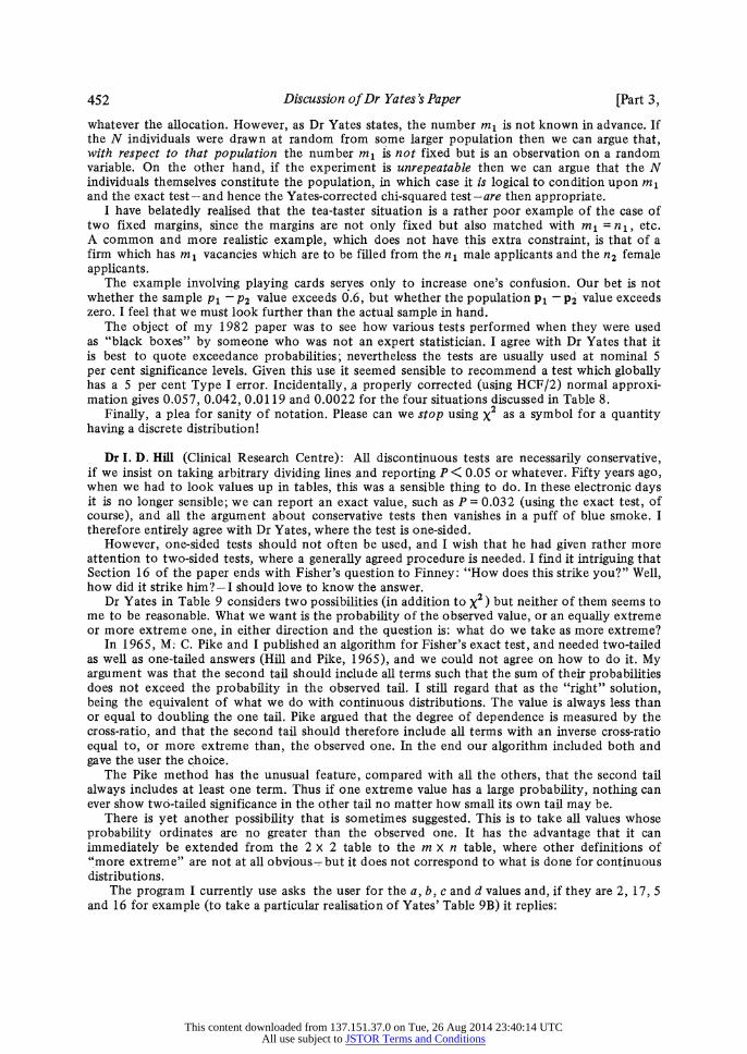
452 Discussion of Dr Yates's Paper [Part 3,
whatever the allocation. However, as Dr Yates states, the number ml is not known in advance. If the N individuals were drawn at random from some larger population then we can argue that, with respect to that population the number ml is not fixed but is an observation on a random variable. On the other hand, if the experiment is unrepeatable then we can argue that the N individuals themselves constitute the population, in which case it is logical to condition upon ml and the exact test-and hence the Yates-corrected chi-squared test-are then appropriate.
I have belatedly realised that the tea-taster situation is a rather poor example of the case of two fixed margins, since the margins are not only fixed but also matched with ml = nl, etc. A common and more realistic example, which does not have this extra constraint, is that of a firm which has ml vacancies which are to be filled from the nI male applicants and the n2 female applicants.
The example involving playing cards serves only to increase one's confusion. Our bet is not whether the sample P -P2 value exceeds 0.6, but whether the population pi - P2 value exceeds zero. I feel that we must look further than the actual sample in hand.
The object of my 1982 paper was to see how various tests performed when they were used as "black boxes" by someone who was not an expert statistician. I agree with Dr Yates that it is best to quote exceedance probabilities; nevertheless the tests are usually used at nominal 5 per cent significance levels. Given this use it seemed sensible to recommend a test which globally has a 5 per cent Type I error. Incidentally, a properly corrected (using HCF/2) normal approxi- mation gives 0.057, 0.042, 0.0119 and 0.0022 for the four situations discussed in Table 8.
Finally, a plea for sanity of notation. Please can we stop using X2 as a symbol for a quantity having a discrete distribution!
Dr I. D. Hill (Clinical Research Centre): All discontinuous tests are necessarily conservative, if we insist on taking arbitrary dividing lines and reporting P < 0.05 or whatever. Fifty years ago, when we had to look values up in tables, this was a sensible thing to do. In these electronic days it is no longer sensible; we can report an exact value, such as P = 0.032 (using the exact test, of course), and all the argument about conservative tests then vanishes in a puff of blue smoke. I therefore entirely agree with Dr Yates, where the test is one-sided.
However, one-sided tests should not often be used, and I wish that he had given rather more attention to two-sided tests, where a generally agreed procedure is needed. I find it intriguing that Section 16 of the paper ends with Fisher's question to Finney: "How does this strike you?" Well, how did it strike him? -I should love to know the answer.
Dr Yates in Table 9 considers two possibilities (in addition to X2) but neither of them seems to me to be reasonable. What we want is the probability of the observed value, or an equally extreme or more extreme one, in either direction and the question is: what do we take as more extreme?
In 1965, M; C. Pike and I published an algorithm for Fisher's exact test, and needed two-tailed as well as one-tailed answers (Hill and Pike, 1965), and we could not agree on how to do it. My argument was that the second tail should include all terms such that the sum of their probabilities does not exceed the probability in the observed tail. I still regard that as the "right" solution, being the equivalent of what we do with continuous distributions. The value is always less than or equal to doubling the one tail. Pike argued that the degree of dependence is measured by the cross-ratio, and that the second tail should therefore include all terms with an inverse cross-ratio equal to, or more extreme than, the observed one. In the end our algorithm included both and gave the user the choice.
The Pike method has the unusual feature, compared with all the others, that the second tail always includes at least one term. Thus if one extreme value has a large probability, nothing can ever show two-tailed significance in the other tail no matter how small its own tail may be.
There is yet another possibility that is sometimes suggested. This is to take all values whose probability ordinates are no greater than the observed one. It has the advantage that it can immediately be extended from the 2 x 2 table to the m X n table, where other definitions of "more extreme" are not at all obvious-. but it does not correspond to what is done for continuous distributions.
The program I currently use asks the user for the a, b, c and d values and, if they are 2, 17, 5 and 16 for example (to take a particular realisation of Yates' Table 9B) it replies:
This content downloaded from 137.151.37.0 on Tue, 26 Aug 2014 23:40:14 UTCAll use subject to JSTOR Terms and Conditions

1984] Discussion of Dr Yates's Paper 453
0 19 7 14 0.0062 0.0062 1.0000 1 18 6 15 0.0553 0.0615 0.9938 2 17 5 16 0.1866 0.2482 0.9385 Observed table 3 16 4 17 0.3111 0.5593 0.7518 4 15 3 18 0.2765 0.8358 0.4407 5 14 2 19 0.1310 0.9667 0.1642 6 13 1 20 0.0306 0.9973 0.0333 7 12 0 21 0.0027 1.0000 0.0027
which gives the individual probabilities, and the cumulative probabilities in each direction. The user can then choose whichever procedure is preferred.
One final question: suppose someone collects data until the number in cell a reaches a parti- cular value, and then stops. All the information is now in the marginal totals. N will follow a negative binomial distribution. What is the correct test for independence?
Professor M. S. Bartlett (Retired): When Dr Yates reviews a problem discussed in 1934, I am among a small group who might celebrate our own little quinquagenary. I have not always seen eye to eye with him, but we seem broadly in agreement with his defence of fixed margins for contingency tables. The exact test makes use of what in my 1937 paper I called "conditional likelihood", when I examined the various sufficiency properties leading to valid tests. However, I regard the "frequency requirement of repeated sampling" as including conditional inferences; and, while I -subscribe to Fisher's search for the most relevant "reference set", I would reject any sets that do not provide a valid sampling frame. (Such a requirement permits inclusion of the t-test, but not the Behrens-Fisher test.)
I do not rule out on principle the possible value of inexact tests based on inequalities, and in the present context such tests include Barnarc's CSM test. But a crucial further point is what happens when Pi / P2; this is very simply illustrated in the extreme case of small Pl, P2 (or alternatively ql, q2). Then a, c and ml become Poisson variables with true means X1, X2 and X1 + X2, say; the ratio a/lm is a binomial variable, with information ml /(PQ) on P = X1 /(X1 + X2), varying with m 1. For general probabilities the situation is more complex, but if 4 = p1q2/(p2q1) the joint probability of a, c is
nlCa n2CC Oa [pm1qi qnn2-m ,
where the factor in square brackets is constant for constant m1 (and nl , n2); hence the conditional probability, given ml, depends only on 4, as noted by Fisher in 1935, though some- what obscurely. Because of this, it would be surprising if the advantageous properties of the conditional probability do not extend to the general Pl, P2 case.
Finally, while it is useful to review the justification of any standard test occasionally, this includes reviewing all the necessary conditions. The dangers of neglecting hidden classifications can be highlighted by Fisher's original example on convictions of "like-sex twins of criminals", classified by zygosity, but apparently not by sex. (There seems some ambiguity about this; in his 1935 R.S.S. paper Fisher does refer to twin brothers, implying all males, yet in the 1958 edition of Statistical Methods he refers explicitly to brothers or sisters.) If anyone is unfamiliar with the dangers of hidden classifications, I recommend Simpson (1951).
Professor M. Aitkin and Mr J. P. Hinde: Dr Yates's first sentence in the second paragraph of his appendix should be expressed in the opposite form: the margins of a 2 X 2 table do in general contain information about the odds-ratio parameter 0 though in large samples this information may be negligible. The marginal totals are not ancillary because their distribution depends on 0. Fisher's statement in Dr Yates's first paragraph is therefore correctly qualified. Conditioning is widely adopted because it seems otherwise impossible to draw conclusions about 0 in the absence of knowledge of some nuisance parameter 0 (e.g. the odds product); the 2 X 2 table being a two-parameter problem.
A new solution to this problem, and to nuisance parameter problems in general, has been pro- posed in Hinde and Aitkin (1984). The approach can be stated succinctly: given a likelihood function L(0, s), we define the canonical likelihoods C1 (0) and C2 () for 0 and / by
This content downloaded from 137.151.37.0 on Tue, 26 Aug 2014 23:40:14 UTCAll use subject to JSTOR Terms and Conditions

454 Discussion of Dr Yates's Paper [Part 3,
XC1 (0) = J L(O, 0 C2 () do
XC2 (G = fL (0o O C1 (0) dO.
For the two-binomials example with n1 and n2 fixed, if 0 = (p, /(I P1 ))/(P2 /(l -P2 )) and =PiP2/((l pi) (1 -p2)) then with observed successes r, and r2
;(O, 0) = 0(r, +r2)/2 0(r - r2)/2 (1 +.\/(0t0))-nj (1 +.\/(OI0))-n2.
The conditional likelihood for 0 given r1 + r2 is
C(0)= (n1, n2 )0 r, /1( n)( n2 )Os
r, r2 s s r, +r2 -S
but L (0, k)IC(0) still depends on 0, as Professor Barnard has also remarked. r1 + r2 is not ancillary, unlike the case of the ratio of Poisson means.
The canonical likelihoods are evaluated in general by numerical integration over a finite grid: in this simple two-parameter case they are given by the principal eigenvectors of the matrix of values of the likelihood function evaluated at the grid-points. For the table n1 = 10, n2 = 8, r, = 2, r2 = 6 the canonical likelihood for 0 is shifted away from 0 = 0 compared to the conditional likelihood: the relative canonical likelihood at 0 = 1 (compared to that at the maximum likelihood estimate 0 = 1/12) is 0.05 18 (using 15-point grids for log (0) and log (p)) while the relative conditional likelihood is 0.0685. The direct likelihood interpretation in either case is that the evidence against 0 = 1 is strong. The Fisher exact probability is 0.0288 for this table, and the exact probabilities of the more extreme tables with r1 = 1 and r1 = 0 are 0.0018 and 0.00002, giving a one-sided significance probability of 0.0306. If the significance probability is doubled for the two-sided test, the evidence against 0 = 1 is not strong.
For the extreme case n1 = n2 = 2, r1 = 2, r2 = 0, the relative conditional likelihood at 0 = 1 is 1/6, the same as the Fisher exact probability of the table. There is not even weak evidence against 0 = 1. The canonical likelihood, efficiently using the information in the marginal totals, gives a relative likelihood at 0 = 1 of 0.026, strong evidence against 0 = 1. This illustrates Barnard's argu- ment: the relative likelihood L(pl,p2)/L(l, 0) is 1/16 at Pi =P2 =P=, and less at any other common value of p: the relative likelihood when correctly averaged over the nuisance parameter must be less than 1/16 at 0 = 1.
As noted above, this procedure applies quite generally to nuisance parameter models: it gives an improvement over the marginal likelihood for a in the N(p, a2) model as well.
Dr D. M. Grove (University of Birmingham): Dr Yates has expressed concern about the number of recent papers which question the wisdom of conditioning on the observed margins of a 2 x 2 table. I conducted a haphazard survey of statistical textbooks, and I can reassure him that in those books the idea of conditioning was accepted without question. Every author, explicitly or implicitly, presented the X2 test as a convenient approximation to an ideal represented by the exact test. But note that in no case was the distinction made between 2 x 2 and larger two-way tables. Dr Yates' paper is not concerned with larger tables, but I think that his argument for the irrelevance of the sampling rule, which he gives towards the end of Section 5, could be applied to larger tables. Moreover, it makes no mention of the parameters.
Leaving parameters out of the argument seems to me to obscure the fact that the 2 x 2 case is a special one. We can express the amount of association in a single odds ratio (as Professor Barnard, Professor Cox and Mr Hinde have all done), and we can follow Barnard or Plackett (1 977) in arguing that there is very little information, if any, in the margins about that odds ratio. In a larger table it is well-known that the conditional distribution can still be written as a function of cross-product ratios-odds ratios-of individual cell probabilities. However, in tables with ordered margins there are many interesting hypotheses which cannot be expressed in terms of such cross-product ratios.
Take, for example, a single multinomial model covering the entire table. If we define r to be the population version of Kendall's rank correlation coefficient, then r > 0 is a natural expression
This content downloaded from 137.151.37.0 on Tue, 26 Aug 2014 23:40:14 UTCAll use subject to JSTOR Terms and Conditions

1984] Discussion of Dr Yates's Paper 455
of the idea of a positive association between the ordered rows and the ordered columns. A natural test of independence against the alternative of positive association could be based on the empirical Kendall rank correlation coefficient, as Professor Armitage (1955) and others have discussed.
It is not difficult to find combinations bf probabilities and margins such that although the Kendall population r is strictly positive the empirical r converges to a negative value in the conditional reference set that is, letting the marginal totals tend to infinity in fixed ratios. The same result holds for other plausible test statistics such as those proposed by Clayton (1974). The corresponding tests are inconsistent. My conclusion is that the argument for conditioning needs to be carefully formulated in such a way as to avoid this kind of inconsistency.
Mr Graham Jagger (Life Science Research Ltd): I would like to make two points. The first concerns the meaning of "more extreme" in the application of Fisher's test. Consider the table (2,3; 4,21). This has expectations (1,4; 5,20). The tables (3,2; 3,22),. . ., (5,0; 1,24) are clearly more extreme than the original in the sense that they depart more and more from expectation. The probability of (2, 3; 4,21) or more extreme tables is, then, 0.254.
There is however, another series of tables, (2,3; 4,21), .. ., (0,5; 6,19), giving a probability of 0.959 for that observed or less extreme. Note that this second case is the one achieved by progressively decrementing the smallest cell in the table, a procedure more or less strongly implied by the authors of most modern statistical texts. Indeed, the manufacturer of my Hewlett-Packard programmable pocket calculator supplies a program that does just that.
It cannot be stressed too strongly that the process of deriving more extreme tables is not formally equivalent to the progressive decrementation of the smallest cell; which procedure is, in general, incorrect. My second point is concerned with the calculation of the two-sided probability. Doubling the single-sided probability of 0.254 derived from my first example yields, using Yates' method (i) a two-sided probability of 0.508. On the face of it this is not unreasonable but difficulties rapidly arise.
Consider the table (2,3; 4,5). This and more extreme tables (as defined above) yields a single-sided probability of 0.657 so method (i), that is, dcwubling, is not an appropriate way of finding the two-sided probability. On the other hand, adding up the probabilities of the tables at the other end of the tail which are as, or more, extreme, gives a two-sided probability of 1. This is Yates's method (ii), and, whatever its shortcomings, always produces a more or less sensible result. I do not understand the "common-sense grounds" upon which Dr Yates condemns this method, especially since method (i) is an even less agreeable alternative.
Perhaps Dr Yates could, in his reply, add to his already fascinating paper with further discussion of this question of two-sided tests.
Dr H. D. Patterson (AFRC Unit of Statistics, Edinburgh): I would like to add my con- gratulations to Dr Yates for a clear and illuminating paper. No question appears to remain un- answered on the single 2 X 2 table but I wonder whether Dr Yates has any advice for us on (a) the combination of several 2 X 2 tables and (b) the use of conditional arguments in other statistical activities, such as the analysis of treatments x places tables of agricultural yields.
The following contributions were received in writing after the meeting. Dr R. S. Cormack (Northwick Park Hospital and Clinical Research Centre): We are all
indebted to Frank Yates for his very clear and cogent restatement of the case for Fisher's model- let us hope that both margins are now well and truly anchored. But there remains the question of the second tail. The consensus of opinion among some distinguished scientists is that Irwin's rule, and related methods of defining the 2nd tail, are not useful. However admirable they may be in theory these methods are not consistently plausible in real life. Yates has found delightful examples of the anomalies that can arise with the Irwin rule-how can the probability of seeing a particular face of the die only once be greater for 31 throws than for 30? Certainly the doubling rule makes more sense here and is consistently plausible in the critical-regions.
Unfortunately, this distinguished assembly is clearly not agreed on the theoretical justification for doubling when the tails are asymmetric. Thus the most pressing need now would seem to be for a way of completing the exact tests which not only gives plausible results, like the doubling rule, but also has a convincing theoretical base. Meanwhile support for the doubling rule must be faute de mieux.
This content downloaded from 137.151.37.0 on Tue, 26 Aug 2014 23:40:14 UTCAll use subject to JSTOR Terms and Conditions

456 Discussion of Dr Yates's Paper [Part 3,
Dr S. E. Fienberg (Carnegie-Mellon University, Pittsburgh, PA-); By casting his defense of Fisher's exact test for 2 X 2 contingency tables in a Fisherian perspective, Dr Yates fails to cite other support for his conclusions. Lehmann (1959, pp. 140-146) notes a strong Neyman-Pearson justification for the two-binomial and independence problems, namely that it is the uniformly most powerful unbiased level a test (with randomization to achieve the nominal level) for equality of the p's. Cox and Hinkley (1974, pp. 134-140) state another version of this result, based only upon achievable levels of significance, and they describe the Fisher test as uniformly most power- ful similar. Despite all of this, I would make a case for the use of the uncorrected X2 statistic and its likelihood ratio counterpart.
Except for cases where n1 and n2 (and by symmetry ml and m2) are quite small, there is not much difference between inferences based on the exact test, and those based on the X2 test. (For these very small sample cases, I too would recommend, and do use in practice, the exact test.) Referring the uncorrected x2 test statistic to the X2 distribution gives a test which for modest- sized samples achieves nominal levels under a multinomial or two-binomial sampling model. Despite what Dr Yates says, the X2 test in this sense is not a conditional test and the continuity- corrected X2 test is conservative. Moreover, the x2 statistic for 2 x 2 tables is a very special case of a test statistic used for a much broader class of problems, in larger two-way and in multi-way tables, representable in terms of loglinear models. The shaky Fisherian arguments about lack of information in the margins to be used for conditioning do not really carry over to these more general settings. For tests,involving multiple degrees of freedom performed for loglinear models, we often wish to partition the X2 statistic or the likelihood-ratio statistic into one-degree-of- freedom components. Using the standard statistics without correction and the corresponding x2 reference distributions seems preferable here. For these reasons, I recommend using the un- corrected X2 test in the 2 x 2 table, except when sample sizes are too small.
The controversy is over the relevance of the exact test, not over whether the continuity- corrected x2 gives close approximations to the exact test (Fienberg, 1980). The crux of Dr Yates's defense of the exact test is Fisher's argument for regarding the margins as ancillary. Since Yates admits that this argument is only approximately true at best, it is not surprising that there is still debate over whether the conditional distribution approach is appropriate.
Professor D. J. Finney (University of Edinburgh): We should be grateful to Dr Yates for his characteristically realistic account of matters that in recent years others have tended to make increasingly obscure. I personally was glad that he has rescued, from correspondence that I had forgotten, an opinion from R. A. Fisher who seems otherwise to have preserved a remarkable reticence on this subject.
Since Dr Yates did not set out to discuss the roles of one-tail and two-tail tests, my remarks are peripheral to his theme; I want to suggest that greater attention ought to be given to the appropriate choice. I have difficulty in finding examples of situations in which a one-tail test makes sense. Textbooks and common practice seem often to imply that, if I am interested only in a deviation in one direction, I should employ a one-tail test. Is a restriction of interest sufficient, even though declared in advance of data acquisition? I believe the correct condition to be "I know that any apparent deviation in the other direction, however large, must be due to chance". For example, in a recent legal battle in an Edinburgh court, one party argued vigorously that cancer death rates had been increased by the adding of fluoride to public water supplies, and insisted that a test of significance should look only at deviations in this direction. They had no interest in indications of a beneficial effect. Yet if a deviation in the direction of reduced mortality among those exposed to fluoride had been several times its standard error, could it conceivably have been automatically rejected as due to chance? (In actuality, when properly calculated, there was a negligibly small deviation in that direction). The complications of X help to emphasize this issue, but of course the logic is equally relevant to other significance tests.
Professor M. J. R. Healy (London School of Hygiene and Tropical Medicine): A common thread running through much of the discussion has been the use of the log odds-ratio or logit difference to measure the amount of association in the 2 X 2 table. As Dr Hill has commented, this provides an alternative definition of extremeness of departure from the null situation, and hence a method of rendering the exact test two-tailed. The probabilities for Tables C and D of Table 9 of the paper are
This content downloaded from 137.151.37.0 on Tue, 26 Aug 2014 23:40:14 UTCAll use subject to JSTOR Terms and Conditions

1984] Discussion of Dr Yates 's Paper 457
C D 0 0.0115 0.0107 1 0.0849 0.0810
6 0.1705 0.1713 7 0.1047 0.1023 8 0.0164 0.0160
To me the main reason against Dr Yates' prescription of doubling the one-tailed probability is simply that the resulting number is not the probability of any definable event.
The lesson I draw from the paper is one Dr Yates has taught me long ago, that a mere significance test is seldom a satisfactory summary of a body of data. The sensible investigator should always seek a quantitative estimate of the amount of association in the table, an interval estimate for preference, and this the log odds-ratio readily provides. From another viewpoint, it gives the necessary peg on which a Bayesian argument can be hung, namely a quantity to which a prior distribution can be ascribed.
A further lesson is that the analysis of discrete data by classical methods is much more tricky than that of continuous measurements. It is a pity that the difference between two proportions is so often chosen as the first example of a statistical technique to be prescribed in the elementary textbooks.
Professor F. D. K. Liddell (McGill University, Canada): Consider samples.n, and n2 from two distinct populations, all N subjected to the same treatment. There can be no doubt (see Section 5 of the paper) that the value of a might take any value, say rl, from 0 to n1, and c any value, say r2, from 0 to n2. Thus, there are two degrees of freedom in the system-with a total of (ni + 1) (n2 + 1) possibilities-instead of one, and that restricted to at most (n1 + 1) possibilities. For given iT, it is well known that P(rl, r2 I nl, n2,ir)=H(rl I R, nl, n2) x Bi(R I N, r), where R = ri + r2: the two terms are the hypergeometric probability of obtaining r, had R been fixed, and the binomial probability of obtaining R out of N with true probability 7r. Ranking the probabilities, for every possible combination of r, and r2, in order of the values of (rl/nl -r2/n2)-or of any plausible statistic that compares Pi and P2 -could lead to a fully unconditional test. It is common practice, when a test procedure depends on an unknown population parameter, to replace that parameter with its sample estimate. Here, replacing the unknown Xr by its ML estimate p = (ml/N) still permits the estimation of the probability of (rI/n1 - r2/n2) for all r, and r2. This process has used one df for estimating p^, leaving the other for comparing pi and P2; however, it has not fixed the ml, m2 margin, and does not appear to involve any illogical step. The test is not strictly unconditional for the estimate of 7r does take account of ml1. Nevertheless, there seems no need to resort to a severely restricted truly conditional test.
Where is the logical failure in this proposal? In other words, if the CDF of (rl/nl -r2/n2) can be determined on the basis of p, why should it not be used for a test, even if the only con- ditioning is the use of ml in obtaining p, and even if the test is more liberal than the (fully) conditional test? The test on these lines I put forward in 1976 did have to be defended, in 1980, but against criticisms of quite different types.
Professor Nathan Mantel (The American University, Bethesda, MD, USA): The erroneous faulting of the Fisher exact test and its continuity-corrected chi square approximation is a curious aberration which just will not go away. Seeming faults with those procedures keep getting dis- covered, rediscovered, and published by new accessions to the statistical profession, and even by well-established professionals.
Perhaps because it is Yates who has now taken up the defense, things will improve, but I doubt it. Other statisticians who also know better are forced to keep quiet inasmuch as no claim of making a new or positive contribution can be made by defenders of the exact test.
Where I would disagree with Yates is in his recommendation for using twice the one-tail probability as a measure of the two-tail probability. He bases this recommendation on the unseemly behaviour he sees for other procedures in an instance where he has been able to shift the cell expectation slightly away from a multiple of 0.5. But whether this is a sound enough basis seems dubious to me. In any case, for tables so large that exact enumeration is unfeasible, Yates would have to make some other recommendation for getting two-tail probabilities.
This content downloaded from 137.151.37.0 on Tue, 26 Aug 2014 23:40:14 UTCAll use subject to JSTOR Terms and Conditions

458 Discussion of Dr Yates's Paper [Part 3,
Because of Yates' emphasis on single-tail testing, he avoids having to define the test statistic relative to which the probability is being sought. The single-tail probability is constant whether our test statistic is the tail probability itself, the absolute deviation from expectation, or the probability of the specific outcome observed. Each of these could give rise to a different value for the two-tail probability, another factor of variation being whether we use exact two-tail pro- babilities, or where suitable, some chi-square-based approximation to that two tail probability.
Among the two-tail probability methods that Yates rejects in favour of twice the one-tail probability is an exact two-tail probability, the test statistic being presumably, as I see it, the absolute deviation from expectation. In his discussion of the work of Haber, Yates notes a "test proposed by Mantel". For the examples Yates gives in Table 9, had Yates applied that chi-square- based test he would have found it to give remarkably close approximations to the exact two-tail probabilities which he had gotten. Still, Yates now rejects such exact two-tail probabilities, though these are the ones customarily used when feasible.
Dr J. A. Nelder (Rothamsted Experimental Station): I have recently completed an annual task of interviewing candidates for the government statistician grade. We usually ask them about X2. Everyone has heard of it, and they all know the "observed-minus-expected" formula. But almost no one knows on what assumption the expected values are expected, and nobody knew this year what X2 measures. They would not know a "proportional" table with a zero X2 if it got up and bit them. I very much hope that in teaching we can move from significance testing towards estimation, with the odds ratio (or some function of it) to measure what is happening in a 2 X 2 table, with the conditional variance to supply an asymptotic s.e. or the exact conditional distribution to supply more exact limits. We can then move on to consider the analysis of sets of 2 x 2 tables in terms of consistency of odds ratios, and so on. A disadvantage of X2 is that it lumps together the extremes of large positive and large negative log-odds ratios in the same tail, something that we should not always want to do. However X2 also has a left-hand tail, when the log-odds ratio is close to zero. Anthony Edwards has pointed out that X2 near zero, the case of "suspiciously close agreement" is extreme in the sense of casting doubt on the variance assumption. Perhaps some data have been rejected, or some other cause of underdispersion is operating. Fisher's re-analysis of Mendel's data is relevant here.
Dr R. L. Plackett (Retired): I regret that a prior engagement prevents me from attending this golden jubilee, and voicing my congratulations to Frank Yates in person. The apparent-simplicity of 2 x 2 contingency tables is deceptive, and conceals several important matters of principle. Two are considered here.
(a) Conditioning on the margins. The combination of numerical examples and statistical intuition in this paper is welcome, not least because any failure to recognjze the force of the arguments for conditioning could be explained by the fact that Fisher and Yates always regarded the need to condition as obvious and presumably therefore not requiring any justification. A consequence of the property that the marginal frequencies provide virtually no inforrmation is that inferences about the cross-product ratio ; should be based on the conditional likelihood function. Fisher (1935) derived an upper fiducial limit on this basis, but he took a different view about estimation: "If we want an estimate of 14 we have no choice but to take the actual ratio of the products of the frequencies observed in opposite corners of the table". I would be interested to know why the unconditional maximum likelihood estimate is so firmly recommended.
(b) Definition of the significance level. In his 1900 paper on chi-squared, Karl Pearson gave actual levels of significance. The use of nominal levels originated when Fisher (1925, chap IV), "owing to copyright restrictions", prepared a new table of chi-squared "in a form which experience has shown to be more convenient". Fisher's argument for defining a two-sided probability as twice the one-tail probability is based on the practice of using nominal levels, which is now criticized as being defective. Another definition was introduced by Neyman and Pearson, who arranged events in order of decreasing probability and calculated the total probability in the tail. A modified version is described by Lancaster (1969, Chap. 3) and Anscombe (1981,. Chap. 12). This is the median probability, which is half the probability of the observed event plus the sum of probabilities for all events less probable, with suitable multiples for equally probable events. I prefer this definition because the expected value of the median probability is 2 under the hypothesis being tested, just as it is for a continuous distribution. In the case of 2 X 2 tables, the median probability is well approximated without using a continuity correction.
This content downloaded from 137.151.37.0 on Tue, 26 Aug 2014 23:40:14 UTCAll use subject to JSTOR Terms and Conditions

19841 Discussion of Dr Yates's Paper 459
The author responded briefly at the meeting; he later replied, in writing, as follows: I should first like to thank all those who contributed to the discussion, or sent in written
comments. As was to be expected many diverse points were raised. I will only comment on them briefly; to do so fully would take more space than is available here.
It is gratifying to find that the need for conditioning on the margins appears to have been accepted by most of the discussants. I am very grateful that Professor Barnard, in proposing the vote of thanks, reiterated his "disavowal" of the CSM test, first made in 1949, and for the account of the correspondence with Fisher that led to this conclusion, particularly as his original paper and the associated paper by Pearson (1947) on quality control continue to be quoted as authoritative by the Neyman-Pearson school.
Section 10 of my paper criticizes Pearson's proposals, but only gives a numerical example for f1 -n2 = 5. After the paper went to the press I wrote a computer program in time to present the results for n, = n2 = 12 (Pearson's values) to the meeting. I reproduce them here in the same format as Table 6, which should be referred to for the full headings.
Odds ratio (a) No verdict (%) (b) Rejection (% Excluding (a)) p1: 2/3 1/2 1/3 p1: 2/3 1/2 1/3
1:1 2.0 0.0 2.0 2.7 3.2 2.7 4 1 0.0 1.0 17.6 42.4 36.0 28.1 00 1.9 19.4 63.2 100 100 100
It is instructive to compare these values with those of Table 6. Note that the best value to aim at for Pi is likely to.be somewhat greater than 1/2.
The only issue on which Barnard differs from me is on the theoretical justification for con- ditioning. He maintains that in the absence of knowledge of the body of the table there is some information on the log-odds ratio in the margins, though this is a trivially small fraction of that from the body of the table except in very small samples, and is affected by the additional unknown error in 4. Does this affect the argument? I maintained it did not, as Pi and P2 are sufficient statistics, and p is merely their weighted mean. Professor Plackett's first query also relates to this issue.
Professor Aitkin and Mr Hinde argue more strongly on the same lines, and have proposed a new solution based on what they term canonical likelihoods. The results they give appear to indicate that their method gives probabilities similar to Barnard's unconditional probabilities. I leave it to others to discuss their proposal when a full account is published.
For reviewing a collection of P values on the same issue Barnard recommends Anscombe's suggestion of counting only half of the probability of the observed value. Professor Plackett also favours this definition of P for discontinuous distributions. This is more or less equivalent to omitting the continuity correction to X2, which, contrary to what I first thought (1934), is necessary when using Fisher's combination-of-probabilities test. I discussed this matter at length in a paper (1955b) on the subject, which was essentially an appendix to a paper (1955a) on the use of maximum likelihood. Dr Patterson may be interested in these papers.
Apart from some-remarks on what he termed "the relatively minor issue" of two-sided tests, which are considered below, Professor Cox mainly discussed problems of estimation that arise when summarising the results from a number of 2 x 2 tables. I will not comment in detail here, as my own paper dealt only with tests of significance for individual 2 x 2 tables. I agree with him that differences in log-odds are not necessarily the most appropriate measure of the difference between two probabilities in all circumstances. He instanced as an alternative Pi - P2. Another alternative is suggested by the inoculation trial described in Section 6. If an estimate of the protection given to those at risk were required, instead of a demonstration that inoculation is always effective, such an estimate would be given by PI= 1 - Pi /p'z where PI is the proportion of those at risk who are protected by inoculation. The numbers in such a trial would of course have to be considerably greater than the 10 of the demonstration trial to give any reliable estimate.
Dr Nelder, also, makes a plea for greater emphasis on estimation. With the general tenor of his remarks I entirely agree. He does, however, like many of the contributors, somewhat uncritically support the use of the odds ratio in all circumstances. In his remarks on x2 the disadvantage that he mentions- that X2 lumps together large deviations occurring on the opposite tails-is a common fault in its use, but is simply avoided by working with + V x2, the deviations in opposite directions being distinguished by the attached sign. These are equivalent to deviates of the
This content downloaded from 137.151.37.0 on Tue, 26 Aug 2014 23:40:14 UTCAll use subject to JSTOR Terms and Conditions

460 Discussion of Dr Yates's Paper [Part 3,
standard normal distribution: values of X2 near zero are equivalent to suspiciously small normal deviates.
Dr Nelder's experience of interviewing candidates reminds me of a similar experience of mine when acting some long time ago as external examiner at a university. In one of the questions I set I asked the students to calculate the value of X2 in a 2 X 2 table, and to comment on the meaning of the result. When the internal examiner sent me the papers he told me that he had reduced the maximum mark for this question, as it seemed easier than all the others. I was somewhat surprised, but the explanation was soon forthcoming. None of the students had made any meaningful com- ment on the values (mostly correct) that they had obtained. I therefore restored the maximum. Presumably these partial failures were due to a defect in the teaching.
Professor Bartlett's contribution puzzles me. After stating that he agrees with conditioning on the observed margins he says he would not rule out "on principle" the CSM test. Thus, to take the (3,0; 0,3) case, he is saying that he agrees with Fisher's exact probability of 1/20 but does not rule out Barnard's probability of < 1/64, which Barnard himself later repudiated. The whole burden of my paper was that it should be repudiated. Nor is this merely a matter of theoretical controversy that does not affect the user of statistics. To take Berkson's example of a clinical trial (Section 12), Kempthorne rightly supported the exact test, but had the experimenter main- tained that the subjects of the trial were in fact a random sample of a much larger population of sufferers from the disease, would Kempthorne have been entitled to use the CSM test? My answer is an emphatic No. The flaw in Bartlett's argument, I think, lies in his statement that Fisher was searching for a relevant "reference set", a Neymanian concept quite different from Fisher's "relevant sub-set".
Bartlett's warning about "hidden, classifications" is of course valid, except that if they are really hidden there is nothing we can do about them when analysing observational data, except to express the hope that they make no material difference. In experimental work, choice of some appropriate system of randomization neutralises the effect of classifications that are unknown and of those whose effects are judged to be likely to be too small to be worth elimination by statistical analysis.
Professor Fienberg is also ambivalent in his choice of tests. If, as he states, he recommends and himself uses the exact test for very small samples, why change the logical basis of the test by switching to the uncorrected x2 for larger samples? His real aim, apparently, is to achieve satis- factory nominal levels. The uncorrected x2 'certainly gives better approximations to these than does the corrected x , as Berkson's investigation shows (Table 9). The differences are, of course, greatest in very small samples.
Professor Liddell falls into the trap of taking as known the estimate of p given by the sample. This is analogous to using the normal distribution instead of the t distribution for testing a mean x, given an estimate S2 of the true variance a2. Would he subscribe to this? I presume that he has not yet seen Professor Barnard's contribution; I hope that this will give him food for further thought.
Dr Upton has based his refutation of conditioning on Pearson's 1947 argument of repeatability. This argument is unconvincing. Comparative trials do not require that the experimental units are selected at random from some defined population. They depend for their validity on random allocation of the units to the treatments. Any such experiment can be repeated, but will in general necessarily be repeated on different units, with fresh randomization. If the units in one or more trials are themselves a random sample from some larger population then any conclusion emerging from the trials can be applied to the population, but tests of significance on the individual experi- ments are unaffected, as I emphasized at the end of Section 6.
Upton also appears to have misunderstood the playing-card example (Section 5). Both players know that each pack contains 26 red cards. The test is that PI - P2 > 0.6. The example was chosen merely to illustrate that knowledge of the margins contributes information on the probability of getting particular outcomes, and therefore to the assessment of the evidence against the null hypothesis Pi = P2. He concludes that we must look further than the actual sample in hand; but this misses the whole point of the arguments for conditioning.
I am glad that he agrees that it is best to quote "exceedance levels" (one-tail, two sided?), but if so why does he pander to users of "black boxes", of which I suppose HCF/2 is an example, without even warning them in his paper of the errors of their ways? And why should X2 not be used for a value which is to be referred to a X2 distribution, just as t and F are used for values
This content downloaded from 137.151.37.0 on Tue, 26 Aug 2014 23:40:14 UTCAll use subject to JSTOR Terms and Conditions

1984] Discussion of Dr Yates's Paper 461
which are to be referred to t and F distributions? I am glad that Dr Grove, in his survey of statistical text-books, found that conditioning was
accepted without question. I have seen at least one in the last year in which the contrary is true, but perhaps friends only draw my attention to what they know will shock me. I agree with him that the 2 X 2 case is special, but to discuss larger tables would be out of place here. It may, how- ever, be worth mentioning that condensation of parts or the whole of larger tables to form a 2 x 2 table is sometimes useful for making quick tests of association before embarking on more formal analysis.
Regarding Mr Jagger's query on two-sided probabilities, obviously the direction of the sum- mation of the probabilities must be the one that gives the lower total. If both directions give totals greater than 0.5 the cell can be regarded as the "central" cell, not belonging to either tail, with a two-sided probability of 1.
To sum up, my view of the function of a test of significance of a single 2 X 2 table is that it should provide a correct measure of the probability P of getting the same or a more extreme set of results by chance, on the assumption that there is no difference in the probabilities, Pi and P2, of the two lines of the table; and that if by probability we mean the concept applied to tosses of a coin or spins of a roulette wheel the only correct measure of P is that given by conditioning on the margins.
Because of the discontinuous nature of the distributions, the combination-of-probabilities test cannot be used on a set of P's, as I mentioned above. But even with adjusted P's (e.g. by omission of the continuity correction) their combination is inefficient because there is no measure of the amounts of information contained in them. For estimates involving several 2 x 2 tables containing small numbers, likelihood must be used. If the numbers in the tables are not too small, normal- theory approximations may suffice.
Finally, some comments on my recommendation that if a two-sided probability is required this should be obtained by doubling the one-tail probability actually observed. This seems the natural thing to do with any continuous distribution, whether symmetrical or not, as it is the probability of the departure from the null value which measures its significance, and, as I pointed out in the paper, this is invariant under transformation. Moreover, when estimation is involved, the direction of the deviation of the parameter from any assumed null value is usually vital. Therefore, in general, one should think in terms of one-tail probabilities, as was implied in the first paragraph of Section 4. This is so whether we are dealing with continuous or discontinuous distributions. It is unfortunate that the customary two-sided tabulations of the normal and t distributions have had the opposite effect.
This conclusion is relevant to Professor Finney's contribution. I would question whether we are ever really in a position to state "I know that any apparent deviation in the other direction, however large, is due to chance". On the contrary, it is our especial duty to draw attention to any evidence contradicting our hopes or beliefs. But it is the one-tail probability that provides the correct measure of the strength of this evidence. Only when tests are being made to check that, for example, two strains of a virus are not materially different, as in Wilson's query to Fisher, or that a coin or die used for gambling is unbiased, can use of a two-sided probability really be justified.
In discontinuous distributions there is the further problem that, except in symmetrical distributions, there will rarely be any value on the opposite tail which has the same one-tail probability as that on the observed tail. The Cox-Hinkley rule (originally, I believe, suggested by Irwin) is then to take the value having the next lower probability to that observed and add this to the observed probability. This seems more sensible than taking the value with the same or next greater deviation (method (ii) of Table 9), which is that widely adopted. But why not take the next higher probability, or better still a weighted mean of the two? Once this latter possibility is considered it is obvious that weights could be chosen so as to give a probability equal to that observed. And then we are back at the doubling rule.
The consequences of using the deviations rule were displayed in Tables 9 and 10 and com- mented on in the text. With the Cox-Hinkley rule (CH) there will almost always be mismatch, except in symmetrical distributions. Consequently the CH probability will almost always be less than double the observed one-tail probability, and can never be greater, as Dr Hill observed. On the other hand the asymmetry of the probabilities will not be obliterated. In Table 9, for example, the CH probabilities for tables C and D are almost identical with one another, and (by chance)
This content downloaded from 137.151.37.0 on Tue, 26 Aug 2014 23:40:14 UTCAll use subject to JSTOR Terms and Conditions

462 Discussion of Dr Yates's Paper [Part 3,
with column (ii) of table D. But as in the deviations method there are sudden large changes in particular probabilities with slight changes in the data. For the four tables with n2 = 59 (table D), 60 (table C), 61, 62, the CH probabilities for a = 1 are 0.102, 0.104, 0.107, 0.170 respectively, compared with the values given by doubling of 0.151, 0.160, 0.169, 0.178. Surely these latter show a more reasonable progression?
Of the discussants, Dr Cormack was the only one who openly condemned the Cox-Hinkley rule, and even he had reservations on the complete validity of the doubling rule. However, Fisher, in his letter to Finney, has opportunely given posthumous support to the doubling rule; his use of nominal levels leads to the same conclusion, by a different route, as that argued above. Professor Cox has also given the doubling rule qualified support, "as the appealing thing to do".
Professor Healy, in private correspondence, dismissed Fisher's suggestion, because of its use of nominal levels, as "pure Neyman-Pearson". In his written contribution he objected that the result of doubling "is not the probability of any definable event". But nor is a one-tail probability, as larger deviations in the same direction are included. There seems no compelling reason for using a strict > rule for the opposite tail, whether our measure is the deviations themselves, their cumulative probability, or the log-odds-ratio. Healy favours this last as an all-purpose mieasure of association, and recommends its use for two-sided tests, in spite of the strong and fully justified objection by Dr Hill, given in his account of his dispute with Dr Pike. I also doubt whether the log-odds-ratio always, or indeed generally, provides the best way of summarising the information in a single small table. A report of the values of Pi and P2, accompanied by a test of significance, is frequently preferable. The assessment of the efficiency of inoculation, mentioned above, provides an example in which the log-odds-ratio would merely confuse. Nor would I like to give any encouragemnent to the Bayesians.
I was disappointed that Dr Mantel was not convinced by my criticism of Haber's results, particularly in view of his long-standing support of Fisher's exact test. Perhaps the further comments on the problem that I have made here will serve to convince him that any of the rules that have been proposed, other than that of doubling, lead to irregular changes in the two-sided probability associated with an observed one-tail probability which is itself little changed by slight changes in the data. Mantel calls such irregularity "unseemly behaviour"; I would say that it indicates that there is likely to be something wrong with our reasoning.
I am not disputing that Mantel's test gives approximations to Haber's exact exceedance probabilities which are better than those given by x2 or x2; I am merely saying that the test is aimed at the wrong target. Surely Mantel's admission that the same observed one-tail probability can give rise to different two-sided probabilities, according to the rule used, is an indication that something is wrong with some or all of the rules.
REFERENCES IN THE DISCUSSION Anscombe, F. J. (1981) Computing in Statistical Science through APL. New York: Springer-Verlag. Armitage, P. (1955) Tests for linear trends in proportions and frequencies. Biometrics, 11, 375-386. Barnard, G. A. (1 982a) Conditionality vs similarity in the analysis of 2 X 2 tables. In Statistics and Probability:
Essays in Honor of C. R. Rao (G. Kalianpur et al., eds), pp. 59-65. Amsterdam: North-Holland. (1982b) Letter to the Editors on 2 X 2 Tables. Appl. Statist., 31, 304-305.
Bartlett, M. S. (1937) Properties of sufficiency and statistical tests. Proc. Roy. Soc. A, 160, 268-282. Clayton, D. G. (1974) Some odds ratio statistics for the analysis of ordered categorical data. Biometrika, 61,
525-531. Cox, D. R. and Hinkley, D. V. (1974) Theoretical Statistics. London: Chapman and Hall. Fienberg, S. E. (1980) Fisher's contributions to the analysis of categorical data. In R. A. Fisher: An
Appreciation (S. E. Fienberg and D. V. Hinkley, eds), pp. 75-84. Hill, I. D. and Pike, M. C. (1965) Algorithm 4: TWOBYTWO. Computer Bull., 9, 56-63. (Reprinted in
ComputerJ. (1979) 22, 87-88; Addenda in ComputerJ. (1966) 9, 212; and (1967) 9, 416. Hinde, J. P. and Aitkin, M. A. (1984) Nuisance parameters, canonical likelihoods and direct likelihood inference.
Research paper No. 4, Centre for Applied Statistics, University of Lancaster. Lancaster, H. 0. (1969) The Chni-squared Distribution. -New York: Wiley. Lehmann, E. L. (1959) Testing Statistical Hypotheses. New York: Wiley. Liddell, D. (1976) Practical tests of 2 X 2 contingency tables. Statistician, 25, 295 -304.
- (1980) Practical tests for comparative trials: a rejoinder to N. L. Johnson. Statistician, 29, 205-207. Simpson, E. H. (1951) The interpretation of interaction in contingency tables. J. R. Statist. Soc. B, 13,
238-241.
This content downloaded from 137.151.37.0 on Tue, 26 Aug 2014 23:40:14 UTCAll use subject to JSTOR Terms and Conditions

1984] Discussion of Dr Yates's Paper 463
Yates, F. (1955a) The use of transformations and maximum likelihood in the analysis of quantal experimnents involving two treatments. Biometrika, 42, 382-403.
-" (1955b) A note on the application of the combination of probabilities test to a set of 2 X 2 tables. Biometrika, 42, 404 -411.
As a result of the ballot held during the meeting the following were elected Fellows of the Society.
Cheesbrough, Anne Griffin, Thomas James Shariff, Nazneen Dagpunar, John S. Hall, Peter Gavin Somchiwong, Malinee Dunn, Richard Jones, Michael Christopher Streeter, Marion Jane Emes, Gerald R. Mukherjee, Dipak Taylor, Wayne A Ghezzo, Ruben H. Rogers, John Wistar
This content downloaded from 137.151.37.0 on Tue, 26 Aug 2014 23:40:14 UTCAll use subject to JSTOR Terms and Conditions