Yiannis Andreopoulos and Mihaela van der Schaar...

DRAFT

1

Adaptive Linear Prediction for Resource Estimation of Video Decoding

Yiannis Andreopoulos* and Mihaela van der Schaar

ABSTRACT Current systems often assume “worst-case” resource utilization for the design and implementation of

compression techniques and standards, thereby neglecting the fact that multimedia coding algorithms require

time-varying resources, which differ significantly from the “worst-case” requirements. To enable adaptive

resource management for multimedia systems, resource-estimation mechanisms are needed. Previous research

demonstrated that on-line adaptive linear prediction techniques typically exhibit superior efficiency to other

alternatives for resource prediction of multimedia systems. In this paper, we formulate the problem of adaptive

linear prediction of video decoding resources by analytically expressing the possible adaptation parameters for a

broad class of video decoders. The resources are measured in terms of the time required for a particular

operation of each decoding unit (e.g. motion compensation or entropy decoding of a video frame). Unlike prior

research that mainly focuses on estimation of execution time based on previous measurements (i.e. based on

autoregressive prediction or platform and decoder-specific off-line training), we propose the use of generic

complexity metrics (GCMs) as the input for the adaptive predictor. GCMs represent the number of times the

basic building blocks are executed by the decoder and depend on the source characteristics, decoding bit-rate

and the specific algorithm implementation. Different GCM granularities (e.g. per video frame or macroblock)

are explored. Our previous research indicated that GCMs can be measured or modeled at the encoder or the

video server side and they can be streamed to the decoder along with the compressed bitstream. A comparison

of GCM-based versus autoregressive adaptive prediction over a large range of adaptation parameters is

performed. Our results indicate that GCM-based prediction is significantly-superior to the autoregressive

approach and also requires less computational resources at the decoder. As a result a novel resource-prediction

tradeoff is explored between: (a) the communication overhead for GCMs and/or the implementation overhead

for the realization of the predictor, and (b) the improvement of the prediction performance. Since this trade-off

can be significant for the decoder platform (either from the communication or the implementation perspective),

we propose complexity (or communication) bounded adaptive linear prediction in order to derive the best

resource estimation under the given implementation (or GCM-communication) bound.

Keywords: Complexity modeling, video decoding, resource estimation, linear prediction

*Corresponding author. Y. Andreopoulos was with the Dept. of Electrical Engineering, University of California, Los Angeles (UCLA). He is now with the Queen Mary University of London, Mile End Road, E1 4NS, London, UK. Tel: +44-20-7882-5345, Fax: +44-20-7882-7997, email: [email protected] . Mihaela van der Schaar is with the Dept. of Electrical Engineering, University of California, Los Angeles (UCLA), Eng. IV, 420 Westwood Plaza, Los Angeles, 90095, CA, USA. Tel. +1-310-825-5843, Fax: +1-310-206-4685, email: [email protected] . The authors greatfully acknowledge the support of the National Science Foundation: NSF CCF 0541867 (Career), NSF CCF 0541453, and NSF CNS 0509522.

DRAFT

2

I. INTRODUCTION The proliferation of media-enabled portable devices based on low-cost processors makes

resource-constrained video decoding an important area of research. However, state-of-the-art video

coders tend to be highly content-adaptive in order to achieve the best compression performance [21]-

[24]. Therefore, they exhibit a highly-variable complexity and rate profile [1] [2] [3]. This makes

efficient resource prediction techniques for video decoding a particularly important and challenging

research topic.

I.A. Related Work

Previous work can be broadly separated in two categories. The first category encompasses

coder-specific or system-specific frameworks for resource prediction. For example, Horowitz et al [1]

and Lappalainen et al [2] analyze the timing complexity of H.264/AVC baseline decoder on two

popular platforms using reference software implementations. Valentim et al [3] analyze the Visual

part of MPEG-4 decoding with the use of descriptors from the encoding parameters and the definition

of worst-case performance results. Saponara et al [4] analyze in a tool-by-tool basis the H.264/AVC

encoding and decoding complexity in terms of memory usage and relative execution time using

profiling tools and compare it to MPEG-4 Simple Profile. Ravasi and Mattavelli [5] propose a tool-

based methodology for complexity analysis of video encoders or decoders using a typical software

description. Most of these approaches are inspired by profiling-based methodologies for execution

time prediction [6] and specialize their application to media decoding algorithms.

The second category of approaches attempts to capture the dynamic resources of video decoders

following on-line adaptation or off-line training approaches that “learn” the features of a particular

system following a generic methodology. For example, Bavier et al [7] predict MPEG decoding

execution time using off-line measurements for typical video sequences and regression analysis.

Dinda and Hallaron [8] experiment with different autoregressive models for host load prediction.

Yuan and Nahrstedt [9] predict video encoding complexity using a histogram-based estimation. Liang

et al [10] analyze processor utilization for media decoding and compared various autoregressive linear

predictors. Similarly, Sachs et al [11] model H.263 encoding time using a variety of linear predictors.

Stolberg et al [12] use a mixed methodology based on prediction techniques and off-line tool-based

analysis and in more recent work [13] propose a generic approach for off-line or on-line linear

mapping of critical function executions to the observed timing complexity. He et al [14] proposed an

analytic model for power/rate/distortion estimation of hybrid video encoding and investigated several

DRAFT

3

tradeoffs using dynamic voltage scaling techniques. Mattavelli and Brunetton [15] derive a broad

framework for estimation of media decoding execution-time based on a linear mapping of encoding-

modes (extracted from the video bitstream) to the execution time of the critical functions of the video

decoder. Off-line measurements were used to define the parameters of the linear mapping. Our

previous work [16] [17] [18] follows a similar approach but, instead of encoding decisions (which are

both algorithm and implementation dependent), it uses compressed-content features, such as motion

vectors and the number of non-zero transform coefficients, which apply in a broader category of video

compression algorithms and are also easily extracted during encoding. In addition, instead of a linear

estimation of decoder functions, we recently proposed a decomposition framework [17] that estimates

platform-independent generic complexity metrics (GCMs), such as the number of motion-

compensation operations, the number of non-zero filter-kernel applications for fractional-pixel

interpolation and spatial reconstruction of a video frame, etc.

I.B. Contribution of the Paper

In this paper we focus on on-line prediction-based approaches for video decoding resource

estimation. Following previous work [17] [15] [10], we attempt to systematically address the

following two basic problems for state-of-the-art video decoding algorithms with rapidly time-varying

complexity profile:

• A general framework for resource-optimized prediction of video decoding execution time under a

given computational bound for the predictor.

• A comparison of autoregressive prediction methods with adaptive linear prediction methods based

on encoder-generated GCMs.

Instead of focusing on worst-case complexity estimation, as it is commonly done in recent video

complexity verifier (VCV) models for MPEG video [3], we follow a recently-proposed VCV model

[19] that focuses on average decoding complexity by introducing variable-size frame buffers and

controlling the decoding delay. This type of VCV model was shown to be significantly better than the

conventional VCV models for streaming video and soft real-time decoding applications, where

additional decoding delay is permitted. This is due to the fact that the model targets systems with

flexible resource utilization rather than systems that are designed based on worst-case performance

guarantees.

For both autoregressive and GCM-based prediction, we examine different configurations for the

adaptive predictor depending on the granularity of the decoder measurement feedback, the complexity

DRAFT

4

requirements imposed at the decoding and the granularity of the input GCMs (if available). In

addition, an optimization framework is proposed that selects the prediction parameters under

prediction-accuracy constraints using offline statistical estimates of the prediction error such that

decoder or transmission resources are utilized in the best possible way.

I.C. Paper Organization

This paper is organized as follows. Section II briefly introduces the video decoding systems of

interest as well as the GCM concept and the various aspects of complexity prediction. Section III

presents the proposed adaptive linear prediction framework for the different cases and quantifies the

various tradeoffs possible. In addition, an optimization framework is presented that can accommodate

resource or information-constrained adaptive complexity prediction using a mixture of off-line

estimations and on-line adaptation. Section IV presents experimental results that compare the various

approaches and Section V analyzes the derived results and outlines possible extensions and

applications. Finally, Section VI concludes the paper.

II. VIDEO DECODING ARCHITECTURES – GENERIC COMPLEXITY METRICS

II.A. Motion-compensated Video Decoding

In MPEG video coding standards, after the motion compensation step the output frames are

categorized as intra-frames (I-frames – denoted as L frames in this paper), predicted frames (P-

frames) from past pictures and bi-directionally predicted frames (B-frames). Both P- and B-frames are

denoted as H frames in this paper. All output frames are spatially-transformed and entropy coded.

The decoder receives the compressed bitstream and after decoding and the inverse spatial transform,

inverts the prediction relationships in order to reconstruct the decoded video frames A . In order to

allow efficient synchronization and random access capabilities to the decoded bitstream, typical

coding structures follow a temporal prediction pattern for a group of pictures (GOP). An example of

the decoding process for a “IBPBPBPB” GOP structure is pictorially shown in Figure 1(a), where we

also highlight the analogy between L and H frames and the conventional I-, P- and B-frame notation

used in MPEG [20]. The superscripts ( , )t n indicate for each frame the temporal-decomposition level

it belongs to (decreased levels t indicate dyadically-increased frame-rate, 0 1t T≤ ≤ + ), as well as

the frame index within each level (n ). Notice that all the H frames (and 1,0TL + ) are first entropy

decoded and then reconstructed spatially by performing the inverse spatial transform prior to their use

in the inverse temporal reconstruction example of Figure 1(a).

DRAFT

5

decoded videosequence 30 Hz

1st level of decomposition15 Hz

2nd level of decomposition 7.5 Hz

L3,0 (I-frame)

L1,0

H2,0 (P-frame)

inverse motion-compensation prediction frame copy step high-pass temporal data for inverse predict step

H2,1 (P-frame) H2,2 (P-frame)

L1,1 L1,2 L1,3

H1,0 (B-frame) H1,1 (B-frame) H1,2 (B-frame) H1,3 (B-frame)

A0,0 A0,2 A0,4 A0,6 A0,1 A0,3 A0,5

frames requiring motion compensation and interpolation frames requiring entropy decoding and spatial reconstruction

A0,7

(a)

decoded video sequence 30 Hz

1st level of decomposition 15 Hz

2nd level of decomposition 7.5 Hz

3rd level of decomposition 3.75 Hz

L1,0

L4,0

L2,0

H1,0

H2,0

H3,0

inverse predict step inverse update step high-pass temporal data for motion-compensated inverse predict and update steps

A0,1 A0,0 A0,3 A0,2

A0,5 A0,4 A0,7 A0,6

L1,1 L1,2

L1,3

H1,1 H1,3H1,2

L2,1

H2,1

frames requiring motion compensation and interpolation

frames requiring entropy decoding and spatial reconstruction

(b)

Figure 1. (a) Example of the temporal reconstruction of conventional MPEG coding using a GOP structure with one I-frame ( 3,0L ), three P-frames ( 2,0 2,1 2,2, ,H H H ) and four B-frames ( 1,0 1,1 1,2 1,3, , ,H H H H ). The decoded frames are indicated by a pyramidal (two-level) spatial wavelet decomposition, although different transforms such as DCT could be employed. (b) Example of MCTF reconstruction using the bidirectional Haar filter [24].

Although the example of Figure 1(a) corresponds to a temporal analysis framework with three P-

frames ( 2,0 2,1 2,2, ,H H H ) and four B-frames ( 1,0 1,1 1,2 1,3, , ,H H H H ), other combinations may utilize

multiple reference frames from the past or the future [21]. In addition, in recent state-of-the-art coding

frameworks, such as the MPEG/ITU AVC/H.264 codec [21], macroblocks of the same video frame

may utilize motion-compensated prediction with variable block sizes and multiple motion vectors

from several reference frames in order to adapt better to the video content characteristics. Although

DRAFT

6

these techniques increase coding efficiency by a significant amount, they pose new challenges for

efficient resource-prediction approaches since a rapidly-varying complexity profile is generated.

Consequently, this demands a generic treatment of the resource-prediction issue that can encapsulate a

variety of encoding parameter settings in an automatic manner.

Scalable video coding architectures based on motion-compensated temporal filtering (MCTF) have

been shown to be a generalization of the previous predictive coding architectures of MPEG [22]. In

particular, at the encoder, video frames are filtered into L (low-frequency or average) and H (high-

frequency of difference) frames by performing a series of motion-compensated predict and motion-

compensated update steps [22]. The process is applied in a hierarchy of T temporal levels. An

example instantiation of the inverse MCTF that reconstructs the input video at the decoder side is

shown in Figure 1(b) (with 3T = ), where, based on the decompressed 4,0L frame and the hierarchy

of H frames, the temporal filtering is inverted (by performing inverse predict and update steps) in

order to reconstruct the decoded video frames A (shown at the top of the figure).

Similarly as before, in state-of-the-art MCTF-based video coding [23] [24], the example of inverse

MCTF illustrated in Figure 1(b) is generalized to motion-compensated temporal filtering using

multiple block sizes with different temporal filters for each macroblock. Finally, it is important to

notice that, when motion-compensated update is disabled in the MCTF process, the decoder structure

becomes equivalent to a conventional predictive framework. Therefore, MCTF-based frameworks can

be seen as a generalization of conventional motion-compensated video decoders.

II.B. Generic Complexity Metrics: A Framework for Abstract Complexity Description

In order to represent at the encoder (server) side different decoder (receiver) architectures in a

generic manner, in our recent work [17] [18] we have deployed a concept that has been successful in

the area of computer systems, namely, a virtual machine. We assume an abstract decoder referred to

as Generic Reference Machine (GRM), which represents the vast majority of video decoding

architectures. The key idea of the proposed paradigm is that the same bitstream will require/involve

different resources/complexities on various decoders. However, given the number of factors that

influence the complexity of the decoder, it is impractical to determine at the encoder side the specific

(real) complexity for every possible decoder architecture. Consequently, we adopt a generic

complexity model that captures the abstract/generic complexity metrics of the employed decoding or

streaming algorithm depending on the content characteristics and transmission bitrate. GCMs are

derived by computing the average number of times the different GRM-operations are executed.

DRAFT

7

Assuming the GRM as the target receiver, we developed abstract complexity measures to quantify the

decoding complexity of multimedia bitstreams [17] [18].

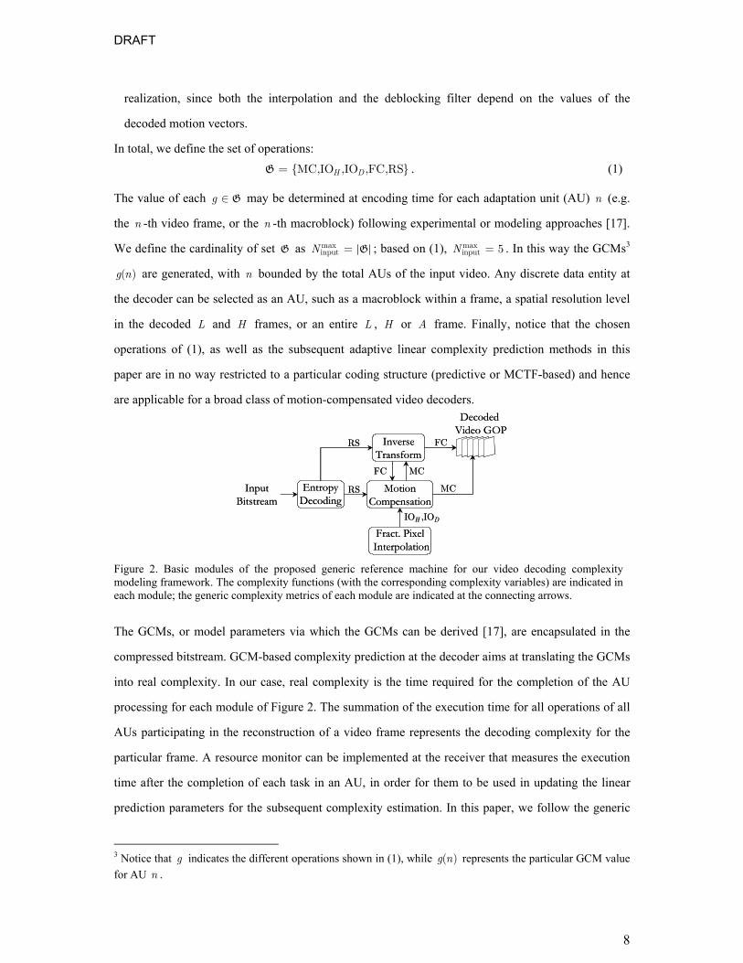
The GRM framework for the majority of transform-based motion-compensated video decoders can be

summarized by the modules illustrated in Figure 2 [17]. The decoder modules, depicted as nodes

connected by edges, communicate via decoded data that are determined by the received bitstream. For

a particular realization of a video decoding algorithm (i.e. using a programmable processor, or an

application-specific media processor, or custom hardware), the decoding complexity associated with

the information exchange between the modules of Figure 2 may be expressed in execution cycles,

processor functional-unit utilization, energy consumption, etc. Based on preliminary experiments that

analyzed several such costs [16], we assume generic operations for each module that are indicated by

the connecting arrows:

• Entropy decoding: the number of iterations of the “Read Symbol” ( RS ) function is considered. This

function encapsulates the (context-based) entropy-decoding of a symbol from the compressed

bitstream.

• Inverse transform: the number of multiply-accumulate (MAC) operations with non-zero entries is

considered, by counting the number of times a MAC operation occurs between a filter-coefficient

( FC ) and a non-zero decoded pixel or transform coefficient1.

• Motion compensation: the basic motion compensation ( MC ) operation2 per pixel or transform

coefficient is the dominant factor in this module’s complexity.

• Fractional-pixel interpolation: the MAC operations corresponding to horizontal or vertical

interpolation ( IOH ), and also the MAC operations corresponding to diagonal interpolation ( IOD ),

can characterize the complexity of this module. Notice that diagonal interpolation is more complex

since it includes both horizontal and vertical interpolation. If a deblocking filter is used at the

decoder, IOH , IOD could incorporate the additional MAC operations for the deblocking filter

1 Notice that, regardless of the use of convolution or faster algorithms (e.g. the lifting-scheme), the inverse transform always consists of filtering operations (similar apply for the case of the discrete cosine transform or other linear transforms) or at least of accumulated bit-shift-and-addition operations (for the case of simplified integer-to-integer transforms). Consequently, non-zero MAC operations are a good metric for a large variety of transform realizations. Notice that GCMs are not expected to capture the precise implementation complexity, which is anyways affected by the implementation architecture specifics, memory accesses, the software/compiler optimizations, etc. They are rather meant as metrics that represent the content-dependent complexity variation for a generic reference machine. 2 In this operation we also encapsulate the decoding of the motion vectors, which, in the vast majority of cases, requires negligible complexity in comparison to motion compensation.

DRAFT

8

realization, since both the interpolation and the deblocking filter depend on the values of the

decoded motion vectors.

In total, we define the set of operations: {MC,IO ,IO ,FC,RS}H D=G . (1)

The value of each g ∈ G may be determined at encoding time for each adaptation unit (AU) n (e.g.

the n -th video frame, or the n -th macroblock) following experimental or modeling approaches [17].

We define the cardinality of set G as maxinputN = G ; based on (1), max

input 5N = . In this way the GCMs3

( )g n are generated, with n bounded by the total AUs of the input video. Any discrete data entity at

the decoder can be selected as an AU, such as a macroblock within a frame, a spatial resolution level

in the decoded L and H frames, or an entire L , H or A frame. Finally, notice that the chosen

operations of (1), as well as the subsequent adaptive linear complexity prediction methods in this

paper are in no way restricted to a particular coding structure (predictive or MCTF-based) and hence

are applicable for a broad class of motion-compensated video decoders.

MotionCompensation

Fract. Pixel Interpolation

EntropyDecoding

InverseTransform

Decoded Video GOP

RS

MC

FC

IO ,IOH D

MC

RS

InputBitstream

FC

MotionCompensation

Fract. Pixel Interpolation

EntropyDecoding

InverseTransform

Decoded Video GOP

RS

MC

FC

IO ,IOH D

MC

RS

InputBitstream

FC

Figure 2. Basic modules of the proposed generic reference machine for our video decoding complexity modeling framework. The complexity functions (with the corresponding complexity variables) are indicated in each module; the generic complexity metrics of each module are indicated at the connecting arrows.

The GCMs, or model parameters via which the GCMs can be derived [17], are encapsulated in the

compressed bitstream. GCM-based complexity prediction at the decoder aims at translating the GCMs

into real complexity. In our case, real complexity is the time required for the completion of the AU

processing for each module of Figure 2. The summation of the execution time for all operations of all

AUs participating in the reconstruction of a video frame represents the decoding complexity for the

particular frame. A resource monitor can be implemented at the receiver that measures the execution

time after the completion of each task in an AU, in order for them to be used in updating the linear

prediction parameters for the subsequent complexity estimation. In this paper, we follow the generic

3 Notice that g indicates the different operations shown in (1), while ( )g n represents the particular GCM value for AU n .

DRAFT

9

approach of assuming that the required time for the processing of every AU in every module of Figure

2 can be measured in real-time. The vast majority of general-purpose processors or DSPs have built-in

registers that can accurately monitor the timing based on the processor built-in clock circuitry [25].

This process is very low-complex and provides accurate measurements. Moreover, the

instrumentation required in the software implementation is minimal and can be done in a similar

fashion for a variety of underlying architectures and software implementations.

III. ADAPTIVE LINEAR PREDICTION OF VIDEO DECODING COMPLEXITY

III.A. Basic Framework

The complexity mapping problem can be formulated as an adaptive linear mapping between the

input GCMs and the real complexity (execution time), or between previous and current complexity.

The k -step linear mapping problem estimates complexity ( )gc n k+ , which corresponds to the

execution time of operation g for AU n k+ , using either the current GCM sequence ( )g n or

previous values of ( )gc n . Specifically:

[ ] 1

0( ) ( ) ( )

P g

g g gp

c n k w p u n p−

=+ = ⋅ −∑ (2)

where: ( ) ( )g gu n p c n p− = − and 0k > (3)

for the case of adaptive linear prediction of the complexity of AU n k+ from previous complexity

measurements, while: ( ) ( )gu n p g n p− = − and 0k ≥ (4)

for the case of adaptive linear mapping of GCMs to the complexity of AU n k+ . The maximum

order of the predictor is indicated by [ ]P g and the predictor coefficients are:

(0) (1) ( [ ] 1)T

g g g gw w w P g = − w . (5)

We define the utilized measurements vector or GCM vector as:

( ) ( ) ( 1) ( [ ] 1)T

g g g gn u n u n u n P g = − − + u . (6)

We additionally define the prediction error for each AU n as:

( ) ( ) ( )g g ge n c n k c n k= + − + . (7)

Based on (2), the last equation becomes:

( ) ( ) ( )Tg g g ge n c n k n= + − u . (8)

DRAFT

10

For each operation g ∈ G , the optimal linear predictor in the mean-square error sense is minimizing 2{ ( )}gE e n . We can identify the (unique) predictor which achieves this by taking the gradient of (8) for

gw and setting it to zero, thereby deriving:

2{ ( )} 0 2 { ( ) ( )} 0g g g gE e n E e n n∇ = ⇔ − =w u , (9)

which can also be expressed as { } ( )g g gu k⋅ =R w r (10)

with { } { ( ) ( ) }Tg g gu E n n=R u u the input’s autocorrelation matrix and ( ) { ( ) ( )}g g gk E n u n k= +r u . If

(3) holds, then (10) corresponds to the [ ]P g -th order autoregressive process with an additional delay

of 1k − samples.

Due to the fact that the optimal solution of (10) requires the knowledge of the autocorrelation of the

input, as well as the inversion of { }guR , we use the popular normalized least mean square (NLMS)

adaptation [26], which periodically updates the coefficients of the predictor based on the normalized

gradient of (9):

2[ ]( [ ]) ( ) 2 ( ) ( )( )

g g g gg

gn l g n e n nnµ+ = +w w uu

, (11)

where 0 [ ] 1gµ< < is the predictor step-size and [ ] 0l g > is the predictor adaptation interval and

2( ) ( ) ( )T

g g gn n n=u u u (12)

is the square of the vector norm of the input. The value of the scaling (step-size) 2[ ] ( )gg nµ u

controls the convergence speed. Higher values lead to faster convergence to the optimal solution

(which is achieved under wide-sense stationarity) and faster adaptation to input changes; however

they also lead to higher predictor-coefficient fluctuations after convergence [26]. If we arbitrarily set

2( ) 1g n ≡u , (13)

then (11) corresponds to the conventional LMS algorithm, which does not require the computation of

the square of the norm of the input, but may exhibit worse convergence properties than NLMS. The

value of [ ]l g of (11) is the predictor update-period, where larger values lead to lower complexity due

to less-frequent updates but also to less accuracy in the adaptation.

Although there are several alternatives to this algorithm [26], (2) and (11) consist of a good approach

for our problem since LMS combines good adaptation properties, stability of convergence with non-

stationary inputs, and low implementation complexity compared to other approaches such as recursive

least squares estimation [26]. Moreover, it was also proven that LMS is H∞ optimal [27], hence,

under proper step-size ( [ ]gµ ) selection, the adaptation minimizes the maximum energy gain from the

DRAFT

11

disturbances to the prediction error. This is an important aspect for our work, since, under bounded

disturbances in the steady-state of the prediction, it guarantees that the energy of the prediction error

for the resource estimation of each decoded video frame will be upper bounded, which means that,

depending on the LMS parameters, the complexity prediction over a time interval (e.g. one GOP)

should be within a certain accuracy range.

III.B. Extensions of Adaptive Prediction

Apart from the order of the predictor ( [ ]P g ), the LMS step-size ( [ ]gµ ) selection and the

predictor-update period ( [ ]l g ), other parameters can also influence the prediction efficiency and the

complexity of the adaptation. The most important is the selection of the appropriate AU granularity

for the input and output of the adaptive prediction. For the complexity prediction of motion

compensation and interpolation operations ( MC( )c n and IO ( )H

c n , IO ( )D

c n ), we are experimenting with

the following three AUs: (a) a video macroblock, (b) one macroblock row, or (c) an entire video

frame. For the inverse transform and entropy decoding ( RS( )c n and FC( )c n ), we are experimenting

with the following two AUs: (a) one spatial resolution of the discrete wavelet decomposition, (b) an

entire decompressed frame. Notice that, in all cases, higher granularity of the utilized measurements

should lead to better prediction results, albeit at the expense of additional complexity at the decoder.

We also investigate whether increased granularity in the provided GCMs assists the linear adaptation.

Since the prediction is done at the decoder side, this comes at a cost of higher communication

overhead for the transmission of these metrics. It is important to mention that in our experiments we

always predict separately for each temporal decomposition level and each frame type. Therefore,

complexity prediction of the L or H frames of each level of the MCTF reconstruction of Figure 1 is

performed separately for each level with a different adaptive linear predictor, leading to

max,predict 2N T= + separate linear predictors for T temporal decomposition levels, where the

increase by two is due to the additional separate predictor for the L frames (“intra” frames), as well as

the adaptive prediction performed at the decoded output video frames (temporal level zero in Figure

1). In addition, we always perform the adaptive prediction over an interval of frames (typically one

GOP). Therefore, for each temporal level t of Figure 1 and each operation g , we have

min{ , }{1,2, ,2 }T t Tk −= … for autoregressive prediction. On the other hand, for the GCM-based

prediction, we have 0k = since the GCMs of each interval of frames (e.g. current GOP) are available

from the video bitstream. In both cases, in order to have causality, the utilized coefficients for the

realization of the prediction are updated only after the frames of the prediction interval have been

DRAFT

12

decoded and the complexity (execution-time) measurements have been obtained, even though

multiple predictor-coefficient updates may occur within a prediction interval. It is also important to

mention that we are always measuring the prediction error for each individual decoded video frame,

even though the prediction interval can be larger (e.g. the duration of one GOP).

Finally, we would like to remark that general combinations of autoregressive prediction (under (3))

and GCM-based prediction (under (4)) could also be envisaged for different time intervals, or for

varying video content characteristics. Alternatively, combinations of autoregressive and GCM-based

predictors for the various temporal decomposition levels could be devised. However, we do not

investigate these mixed estimations in this work.

III.B.1 Generalization of Adaptive Prediction Parameter Set

Let ( , )q g t= be a set-element indicating the prediction operation-type (g ) and the temporal

level ( t ) of the prediction out of the entire set { },{0, , 1}T= +…Q G of possible choices. For each

set element ( , ), q g t q= ∈ Q , we represent the AU granularity (sampling) of the input and output of

the adaptive prediction by [ ]i qn , with maxsample,[ ] {1, , }qi q N= … , i.e. the subscript i of AU n (for

operation g at temporal level t ) increases with the increase in the AU granularity. In the presented

experiments, following the previous description in the beginning of Subsection III.B we have

maxsample, 3qN = for { }(MC, ),(IO , ),(IO , )H Dq t t t= , and max

sample, 2qN = for { }(RS, ),(FC, )q t t= . Notice

that, for all cases, 1n corresponds to the coarsest AU granularity, which is one entire decompressed

video frame 10,nA . Moreover, if the provided granularity for the input GCMs is lower than that of the

desired granularity for the predicted complexity, bilinear interpolation or sample-and-hold techniques

are used to increase the sampling rate of the input GCMs. The generalized adaptive complexity

prediction of AU [ ] [ ]i q i qn k+ is now formulated as:

[ ]

[ ] 1

[ ] [ ] [ ] [ ] [ ]0

( ) ( ) ( )i q

P q

q i q i q q i q q i q i qp

c n k w p u n p−

=+ = ⋅ −∑ . (14)

The adaptation of the predictor is performed as:

[ ] [ ] [ ] [ ]2[ ]

[ ]( [ ]) ( ) 2 ( ) ( )( )

q i q q i q q i q q i qq i q

qn l q n e n nnµ+ = +w w u

u. (15)

The last two equations represent a very large number of possibilities since the cardinality of the set of

choices is4:

4 In (16), the second term is 1T + and not 2T + since some operations do not occur for 0t = or

2T T= + as it will be explained in the subsection III.C.

DRAFT

13

( )maxinput 1N T= ⋅ +E (16)

and the parameters that can be adjusted are [ ]i q , [ ]l q and [ ]P q .

For example, if the prediction is performed for an interval of one GOP, for 4T = (typical parameter

for MCTF-based coders), and maxinput 5N = (following (1)), we get 25=E . Then, even for a fixed

predictor order [ ]P q , for two possible values for each of the [ ]i q , [ ]l q parameters, we get over 1310

possible combinations of predictor assignments for each GOP of decoded video. Each parameter

assignment requires certain computation for the prediction realization and can lead to different

expected prediction efficiency. Hence, under a general optimization framework for complexity

prediction, all possible assignments should be considered.

III.B.2 Generalization of the Adaptive Prediction Time Interval

Depending on the particular application, the proposed adaptive prediction of video decoding

complexity may be applicable for the derivation of the expected complexity for one frame, or for a

group of decoded frames. This can be expressed as:

depend[ ]

dependout 1 [ ]( ) ( )

qi q

q i qq n

c n c n∀ ∈ ∈

= ∑ ∑Q d

(17)

where ( , )q g t= (q ∈ Q ) was defined previously, out 1( )c n is the output complexity estimate for AU

(decoded video frame)5 10,nA , qd is the set containing the indices to the AUs, denoted by depend[ ]i qn ,

which are utilized for the construction of the output AU 1n (i.e. the temporal dependencies of AU

1n ), and the complexity of each individual AU depend[ ]i qn , denoted by depend

[ ]( )q i qc n , is defined as in (14).

Notice that the cardinality of each set qd , denoted by qd , depends on the AU sampling choice [ ]i q .

As an illustrative example, if we assume that q∀ ∈ Q we select [ ] 1i q = for the instantiation of the

MCTF decoding depicted in Figure 1(b), for the complexity for the reconstruction of frame 0,0A , i.e.

out(0)c , we have: ( ,0)={1}gd and ( ,{1,2,3})={0}gd for ={MC, IO , IO }H Dg and ( ,{1,2,3,4})={0}gd for

={RS,FC}g . In addition, for the complexity of the reconstruction of the entire GOP, out 1( )c n with

1 {0, ,7}=n … , we have ( ,1) {0,1,2, 3}g =d , ( ,2) {0,1}g =d , ( ,3) {0}g =d for ={MC, IO , IO }H Dg and,

( ,4) {0}g =d for ={RS,FC}g .

It is important to emphasize that, q∀ ∈ Q , the complexity depend[ ]( )q i qc n in (17) has a different

granularity expressed by [ ]i q . As a result, depending on the choices for [ ]i q in (14), the output of (17)

changes and the cost (in terms of implementation or communication overhead) for deriving this

5 Notice that in outc the subscript of the AU n is always one since in this paper we are interested in predicting the complexity at the coarsest AU granularity, which is at the video frame granularity.

DRAFT

14

complexity estimate varies. The analytical formulation of this cost is the topic of the following

subsection.

III.C. Complexity and Information Requirements for Adaptive Prediction

Following the generalized adaptive prediction of (14), (17), for every decoded video frame

10,nA we need the following average number of operations (MACs):

depend[ ]

compute 1 coeff[ ]O ( ) [ ] O [ ][ ]

qi qq n

P qn P q ql q∀ ∈ ∈

= + ⋅ ∑ ∑dQ

, (18)

with qd defined as previously for (17) and

coeff

2, if NLMS is usedO [ ]

1, if LMS is used q

= , (19)

where the case of NLMS corresponds to (12), while LMS is the case where the simplification of (13)

is used. In (18), we account for [ ]P q MAC operations for (14) and [ ]P q operations for the predictor

update every [ ]l q samples. In addition, we account for [ ]P q operations for the term 2[ ]( )q i qnu in (15)

for the case of NLMS. Notice that [ ]qµ is predefined and fixed for a particular predictor (as discussed

in the experimental results section of the paper). Hence, the division of [ ]qµ by 2[ ]( )q i qnu in (15) is

assumed to be performed by rounding and a lookup table and is not included in the complexity

estimation of (18), since the comparison of division and multiplication operations is machine

dependent. However, even under the inclusion of the division operation, the predictor complexity

results are simply offset by the machine-specific division overhead.

Notice that the outer summation of (18) operates 2T + times for each operation g . However,

depending on the operation, 0t = or 1t T= + may entail no complexity. This is because we have

(MC, 1)T+ ∅d , (IO , 1)H T+ ∅d , (IO , 1)D T+ ∅d , i.e. there are no motion compensation or interpolation

operations for the construction of the 1,0TL + frame, and also (RS,0) ∅d , (FC,0) ∅d due to the fact

that the output video frames 10,nA do not require entropy decoding operations or inverse spatial

transform operations.

For complexity prediction with GCMs at the decoder side, the server must transmit

GCM 1I ( ) q

qqn

r∀ ∈= ∑

Q

d (20)

GCMs, where qr is the ratio of complexity measurements to GCMs for each operation g of each

temporal level t . Typical values are 1qr = , or we may set (MC, )tr , (IO , )H tr , (IO , )D tr equal to the

number of macroblocks within a video frame and (RS, )tr , (FC, )tr equal to the number of spatial

resolutions of a video frame and bilinearly interpolate (or sample-and-hold) in order to produce the

DRAFT

15

required GCM granularity at the receiver side. Although the calculations of this subsection were

presented under the assumption of a total of T temporal reconstructions, low frame-rate decoding

may be accommodated by excluding the calculations for min0, , 1t t= −… , where mint the lowest

reconstructed temporal level. Low-resolution decoding (for scalable coders) can be accommodated in

a similar manner.

Finally, concerning the expected prediction error, similar to (7), we can formulate the error of the

generalized complexity prediction for decoded frame 10,nA as:

depend[ ]

depend dependout 1 [ ] [ ]( ) ( ) ( )

qi q

q qi q i qq n

e n c n c n∀ ∈ ∈

= −∑ ∑Q d

, (21)

which becomes

depend

[ ][ ]

[ ] 1depend depend

out 1 [ ] [ ] [ ][ ] [ ]0

( ) ( ) ( ) ( )i qqi q

P q

q q i q q i q i qi q i qq pn

e n c n w p u n p k−

∀ ∈ =∈= − ⋅ − −∑ ∑ ∑

Q d

(22)

The last equation indicates that the contribution of each operation g of each temporal level t to the

output prediction error out 1( )e n may differ. In fact, the intermediate prediction errors of (22), along

with the required complexity or information overhead for the realization of the prediction (eq. (18)–

(20)) may be used as the driving force of a low-complexity optimization mechanism for the adaptive

selection of parameters of the adaptive complexity prediction formulated by (17). This is the topic of

the following subsection.

III.D. Resource-constrained Adaptive Linear Complexity Prediction

Based on the previous definition of the adaptive prediction, for each ( , )q g t= , we can modify

the AU granularity ( [ ]i q ), the prediction update period ( [ ]l q ), the predictor order ( [ ]P q ) and the

predictor step-size ( [ ]qµ ). In this paper, the optimal predictor order [ ]P q and step-size [ ]qµ were

selected based on exhaustive experimentation with a large set of possible values, as it will be

explained in the experimental section of the paper. Consequently, we are focusing on the [ ]i q and [ ]l q

parameters here. In principle, we would like to select the parameters that would minimize the output

prediction error out 1( )e n given in (22). However, this may entail high computational complexity or

high information requirements (under the calculations of (18) and (20), respectively). Moreover,

under the flexible VCV model [19] adopted in this work, the complexity (timing) bound for each

group of output frames (AUs) may be satisfied without the best-possible prediction accuracy and

therefore the resource predictor may be realized with less computation. After making this key

DRAFT

16

observation, we would like to obtain the best possible prediction accuracy under a certain predictor-

complexity bound:

out 1 compute 1 bound 1( [ ], [ ]) arg min ( ) s.t.O ( ) O ( )qi q l q e∗ ∗∀ ∈ = ≤n n nQ , (23)

where the optimal solution ( [ ], [ ])i q l q∗ ∗ is a point in the Q -dimensional hyper-set of possible

parameters QP , which is bounded by:

maxsample,, 1 [ ] , 1 [ ]q qq i q N l q∈ ≤ ≤ ≤ ≤Q d . (24)

In the last equation we selected qd as the maximum predictor update period ( [ ]l q ) in order to ensure

that the predictor is updated at least once during each group of AUs qd .

Notice that (23) represents the most general form of the problem that, under a given predictor

complexity compute 1O ( )n , simultaneously adapts all the available prediction parameters in order to

minimize the expected prediction error over a finite interval of future decoded video frames 1n . The

problem can be similarly defined for the minimization of the information requirements GCMI :

out 1 GCM 1 bound 1( [ ]) arg min ( ) s.t. I ( ) I ( ) qi q e∗∀ ∈ = ≤n n nQ . (25)

The optimization of (25) is simpler than that of (23) as, from the definition of GCMI of (20), it only

involves the selection of the GCM granularity [ ]i q . As a result, we shall focus on (23) in the

remainder of this paper, since simplified solutions to (23) can be applied for the case of (25) as well.

In order to solve (23) we follow an off-line estimation and pruning approach and then during the on-

line estimation we select the appropriate prediction parameters based on the off-line estimates. In this

way, the off-line optimization part can entail high complexity while the complexity of the on-line

estimation is only stemming from the adaptive filtering.

We start by separating the prediction error into smaller parts:

out 1 out( ) ( )qq

e e∀ ∈

= ∑nQ

d , (26)

where each intermediate error out( )qe d is defined based on the correspondence of (26) with (21). As

seen by (26), each of these intermediate errors is equally important in the output error metric.

Moreover, for each choice of { [ ], [ ]} qi q l q ∀ ∈Q , based on (18), we can analytically establish the

resulting computational impact in the adaptive complexity prediction realization. It is straightforward

to observe from (18) that the required computation monotonically increases with increasing [ ]i q and

with decreasing [ ]l q . Under the assumption6 that the expected error can be reliably estimated off-line

6 This will be analyzed in the following subsection (Subsection III.E).

DRAFT

17

for the possible choices of [ ]i q and [ ]l q , the optimization of (23) can be performed with dynamic

programming techniques, as explained in the following.

Each point ( [ ], [ ])i q l q ∈ QP (where P Q is the initial parameter hyper-set) is associated with its

corresponding computation/prediction-error (C-P) point ( )compute ( [ ], [ ])O , i q l qe . Recall that each

( [ ], [ ])i q l q is selected within the bounds set in (24). Assuming that all possible alternatives are to be

utilized in our complexity prediction system, for each q ∈ Q we initially obtain maxsample,q qN ⋅ d C-P

points, which form the initial set of valid C-P points, denoted by qV . During a pruning stage, for each

q ∈ Q we remove from qV all C-P points for which there exists another C-P point in qV with lower

or equal computational requirements and lower prediction error.

In the second phase, we group together all admitted points in sets [ ]q q∀ ∈QV into the sets ( , )tGV , by

summing up the admitted points of qV that correspond to the same temporal level, i.e.:

( ) ( )compute compute( [ , ], [ , ]) ( [ , ], [ , ])O , O ,i t l t i g t l g tg

e e∀ ∈

= ∑G GG

. (27)

The pruning stage is repeated for all C-P points of ( , )tGV . Finally, in the third stage we group all

admitted points of ( , )tGV for all levels:

( ) ( )1

compute 1 out 1 compute( [ ], [ ]) ( [ , ], [ , ])0

O ( , ( ) O ,T

i l i t l tt

e e+

== ∑n n

Q Q G G (28)

where the C-P points ( )compute 1 out 1 ( [ ], [ ])O ( , ( ) i len nQ Q

are pruned as before in order to form the set of

admissible points QV . Every C-P point that is finally admitted to QV forms a potential (optimal)

solution, depending on the bound set on the predictor complexity by (23). Notice that the grouping

and pruning process described previously can be performed off-line if estimates for all C-P points are

available. In addition, all the admitted points can be off-line sorted in ascending order with respect to

the expected prediction error (and, correspondingly, in descending order with respect to the predictor

complexity), thereby creating the sorted list of admissible points sortedQV . As a result, the on-line

optimization simply amounts to selecting the C-P point in sortedQV with the complexity that is closest

to bound 1O ( )n . This ensures negligible complexity overhead for the optimization of (23).

III.E. Off-line Estimation of the Expected Prediction Error under Predictor-

parameter Adaptation

Having a reliable off-line estimation of the expected error for a particular set of predictor

parameters is a crucial aspect of the optimization framework of the previous subsection, because,

under wrong error estimates, a suboptimal point of the parameter hyper-set QP may be selected. Our

expected error estimation is performed off-line based on a collection of training data and the bootstrap

DRAFT

18

principle [28]. Since the statistics of the prediction errors are dependent on the prediction parameters

and the utilized video coding scheme, conventional statistical modeling approaches can be very

complicated and also application-specific. The bootstrap approach calculates confidence intervals for

parameters where such standard methods cannot be applied [28]. It is essentially a computerized

method that replaces statistical analysis with computation, as it will be explained in the following.

We collect off-line experimental measurements using 7 typical video sequences decoded at 13

equidistant average bitrates between the values of interest (200-1500 kbps). We also fix our

experimentation in the prediction of the decoding time of each frame of an entire GOP. Our test case

uses 4T = temporal levels of an MCTF-based coder, a separate adaptive predictor per temporal level

and per operation type (set G of (1)), as well as a separate predictor for the L frame of each GOP and

for the decoded video frames (temporal level zero). We applied the AU sampling granularities

described in introduction of Subsection III.B and, for each sampling granularity three different

predictor update periods were tested, i.e. [ ] {1,2, 4}l q = samples. The entire parameter space explored

is presented in Figure 3. Notice that, depending on the chosen application, a different (even larger)

parameter space could be used with the same methodology for off-line prediction error estimation. decoded frames

(only for)

0t = 1t = 2t = 3t = 4t = 5t =framesL

={MC, IO , IO }H Dg (only for )={RS,FC}g

: MB sampling: not applicable

={MC, IO , IO }H Dg={RS,FC}g

: MB-row sampling: spatial resolution

={MC, IO , IO }H Dg={RS,FC}g : decoded frame


[ , ] 1l g t = [ , ] 2l g t = [ , ] 4l g t =

[ , ] 3i g t = [ , ] 2i g t = [ , ] 1i g t =

decoded frames

(only for)

0t = 1t = 2t = 3t = 4t = 5t =framesL

={MC, IO , IO }H Dg (only for )={RS,FC}g

: MB sampling: not applicable


: MB-row sampling: spatial resolution

={MC, IO , IO }H Dg={RS,FC}g : decoded frame


[ , ] 1l g t = [ , ] 2l g t = [ , ] 4l g t =

[ , ] 3i g t = [ , ] 2i g t = [ , ] 1i g t =

Figure 3. Explored parameter space.

Under the selected parameter space of Figure 3, we decoded the test video material at the bitrates of

interest and generated off-line decoding time measurements for each operation g , as well as their

prediction with all possible predictor configurations. For each temporal level and each g ∈ G ,

out( )qe d was estimated as follows.

Each measurement set { ,( [ ], [ ])}q i q l qM consists of m pairs of measurements of timing complexity and

predicted values under the particular choice ( [ ], [ ])i q l q , indicated by mc and mc , respectively. In total,

DRAFT

19

for each { ,( [ ], [ ])}q i q l q , we have measure1 m N≤ ≤ pairs of measurements, with

( ) { }min ,measure 13 7 2 t TN F= ⋅ ⋅ under the chosen settings (7 sequences, each consisting of 256F =

total video frames, decoded at 13 different bitrates). We calculate the mean absolute prediction error

as:

measure

0( [ ], [ ])

measure 1

1 N

mmi q l qm

e c cN =

= −∑ , (29)

Subsequently, based on a pseudo-random number generator, we resample ( ,( [ ], [ ])}q i q l qM with

replacement and produce a resampled set 1{ ,( [ ], [ ])}q i q l qM containing measureN pairs of points. The new

mean prediction error, denoted as 1( [ ], [ ])i q l qe , is calculated as in (29), with ( ) 1

{ ,( [ ], [ ])}, mm q i q l qc c ∈ M . This

process is repeated for a total of bootstrapN iterations, thereby generating the set:

{ }bootstrap1( [ ], [ ]) ( [ ], [ ]) ( [ ], [ ]), , Ni q l q i q l q i q l qe e= …B (30)

of off-line generated measurements of the mean prediction error for the particular parameter choice

( [ ], [ ])i q l q . Notice that several pairs may be duplicated during the resampling process, thereby creating

a different bias for the resampled set of measurements, which is a key aspect for the utilized bootstrap

parameter estimation technique. These measurements are sorted in increasing order bootstrap1 2

( [ ], [ ]) ( [ ], [ ]) ( [ ], [ ])N

i q l q i q l q i q l qe e e≤ ≤ ≤… where ( [ ], [ ])mi q l qe is the m -th smallest element of ( [ ], [ ])i q l qB . We

define the sorted measurement set as ( [ ], [ ])i q l qB .

If we desire 100ε ⋅ bootstrap confidence interval, then the expected mean prediction error is bounded

by ( [ ], [ ]) ( [ ], [ ])( , )i q l q i q l qe eα β , with the indices ,α β defined as:

( )

bootstrap1

2N εα − =

, (31)

bootstrap 1Nβ α= − + . (32)

Figure 4 shows an example of the (sorted) bootstrap-estimated error for the MC operations of

temporal level one under various granularities for the prediction. As shown there, we performed

bootstrap 1000N = iterations for each case. In our experiments, we adapt the confidence interval

dynamically based on the previously-observed errors. In this way, although the error estimation is

performed off-line, our “confidence” on the estimate is adapted on-line by matching the off-line

(bootstrap) estimate with the observed error estimate of the previously-predicted frames. Since

different confidence intervals have to be considered and this may alter the points excluded from the

pruning process of the previous subsection, we selected 10 values for the confidence interval, defined

by {0.1,0.2, ,1.0}ε = … , and performed the pruning process under each one. Once the derived indices

,α β are derived for each interval ε based on (31), (32), we define the bootstrap mean error for this

DRAFT

20

interval (for each operation g at each temporal level t and each predictor parameter choice

{ [ , ], [ , ]}i g t l g t ) as:

out ( [ ], [ ])1( ) i

q i q l qi

e eβ

αα β ==

− ∑d , (33)

In total, during the on-line complexity prediction process, the optimal predictor is selected based on

(23), with the expected error out 1( )e n found from the bootstrap estimates under the appropriate

confidence interval for every q , denoted by [ ]qε . After the video frames are decoded and the

complexity prediction error is calculated based on the experimental measurements, the confidence

interval is readjusted according to the mismatch between out ( , )( )g te d and the measured error out( )qe d .

Although we used the first sample moment for our optimization process (mean estimate of (33)),

higher sample moments such as the expected error variance could be estimated and used in the

proposed framework.

Finally, it is important to emphasize that, although we selected the uniform distribution for the

resampling of the bootstrap process (via the use of a pseudo-random number generator), if explicit

knowledge is given for the probability distribution function (pdf) of the errors of a particular

parameter choice ( [ ], [ ])i q l q , this pdf can be used for the resampling process in order to increase the

bootstrapping estimation performance.

0 100 200 300 400 500 600 700 800 900 1000400

600

800

1000

1200

1400

1600

Boo

tstra

p er

ror (

tics)

Bootstrap iteration (sorted)

MC operations (fixed predictor order, unitary adaptation interval)

per frameper macroblock rowper macroblock

0.8ε =

Figure 4. Example of the derived off-line bootstrap estimates for the MC operations at temporal level 2t = (under a given predictor order and predictor adaptation interval of one sample, with bootstrap 1000N = ). An example of a confidence interval is indicated as well.

DRAFT

21

IV. EXPERIMENTAL EVALUATION

IV.A. GCM-based Prediction versus Autoregressive Prediction

We first indicate the achieved prediction performance and average complexity requirements for

the predictor (in terms of MAC operations per video frame) for different configurations. The results

are seen in Table 1 for the GCM-based adaptive prediction and in Table 2 for the autoregressive

adaptive prediction. The numbers in parentheses indicate the required number of MAC operations for

the realization of the complexity predictor, calculated based on (18) for each predictor granularity and

adaptation interval. We used seven MPEG CIF sequences (“City”, “Football”, “Raven”, “Sailormen”,

“Tempete”, “Mobile” and “Foreman”, of 300 frames each) with a replay rate of 30 Hz, decompressed

at an average of 512 Kbps (variable-bitrate) with the advanced MCTF-based video decoder [24] used

in our previous experiments [18] [24], which combines multi-frame advanced motion compensated

prediction with variable block sizes and context based entropy coding. Our choice of the particular

decoder stems from three factors: (i) complexity prediction within an MCTF-based framework is

more challenging than in predictive coding due to the more complex interactions required for the

decoding of each GOP; (ii) the decoder of [24] performs advanced multiframe multihypothesis motion

compensation with variable block sizes and in this way it resembles state-of-the-art video coding

systems such as the MPEG AVC/ITU H.264; (iii) by using the decoder of [24], this paper is directly

linked to our previous related work in this area [17] [18].

Notice that, since the GCM framework of Figure 2 is applicable to essentially all transform-based

motion-compensated video coding schemes, the proposed framework is only tied to a particular

decoder in terms of the GCM granularity and the number of different frame types chosen. Both of

these features must be selected based on the decoder features. For example, for a block-based

transform system with predictive coding using I, B, and P frames (i.e. an MPEG-1/2/4 coder or

AVC/H.264), the high granularity for the FC operations would be at the macroblock level instead of

the spatial resolution chosen for the discrete wavelet transform. In addition, we would set 2T = as

shown in the example of Figure 1(a). Hence, customization to any decoder can be performed by

appropriately selecting the GCM granularity and the number of different complexity predictors based

on the decoder characteristics, and the proposed complexity prediction methodology follows in a

straightforward manner.

The chosen decoding algorithm [24] for the validation experiments of this paper was implemented in

C++, compiled with Microsoft Visual Studio 6.0 in release mode, and executed in the Microsoft

DRAFT

22

Windows XP environment in a Pentium-IV system. With all the advanced coding options enabled

(long temporal filters, multihypothesis motion-compensated prediction and update, etc.), real-time

decoding was not possible without additional software optimization. Hence, similar to prior work [3]

[19], we resorted to simulation-based results. In Table 1 and Table 2 we present the average error-

over-measurement (EM) power ratio for each of the generic-operations presented in Subsection II.B

as well as the computational complexity of each predictor in terms of average MAC operations per

decoded video frame.

All measurements of prediction errors are obtained per decoded video frame. The prediction estimates

the complexity of the following GOP based on the GCMs of the GOP (GCM-based prediction) or the

previous GOP’s complexity (autoregressive prediction) as seen in (14). In particular, for every

temporal level t in (14), (15), we have ( , ) [ , ] [ , ] [ , ] [ , ]( ) ( )g t i g t i g t i g t i g tu n p g n p− = − and [ , ] 0i g tk = ,

[ , ] 1i g tl = for the GCM-based prediction, and ( , ) [ , ] [ , ] [ , ] [ , ]( ) ( )g t i g t i g t g i g t i g tu n p c n p− = − and [ , ] 1i g tk = ,

[ , ] 1i g tl = for the autoregressive prediction. During the GOP decoding, in both cases the predictor is

adapted following (15), and at the end of the GOP the predictor to be used for the following GOP is

updated. Obviously, more frequent updates of the predictor lead to better prediction accuracy, but the

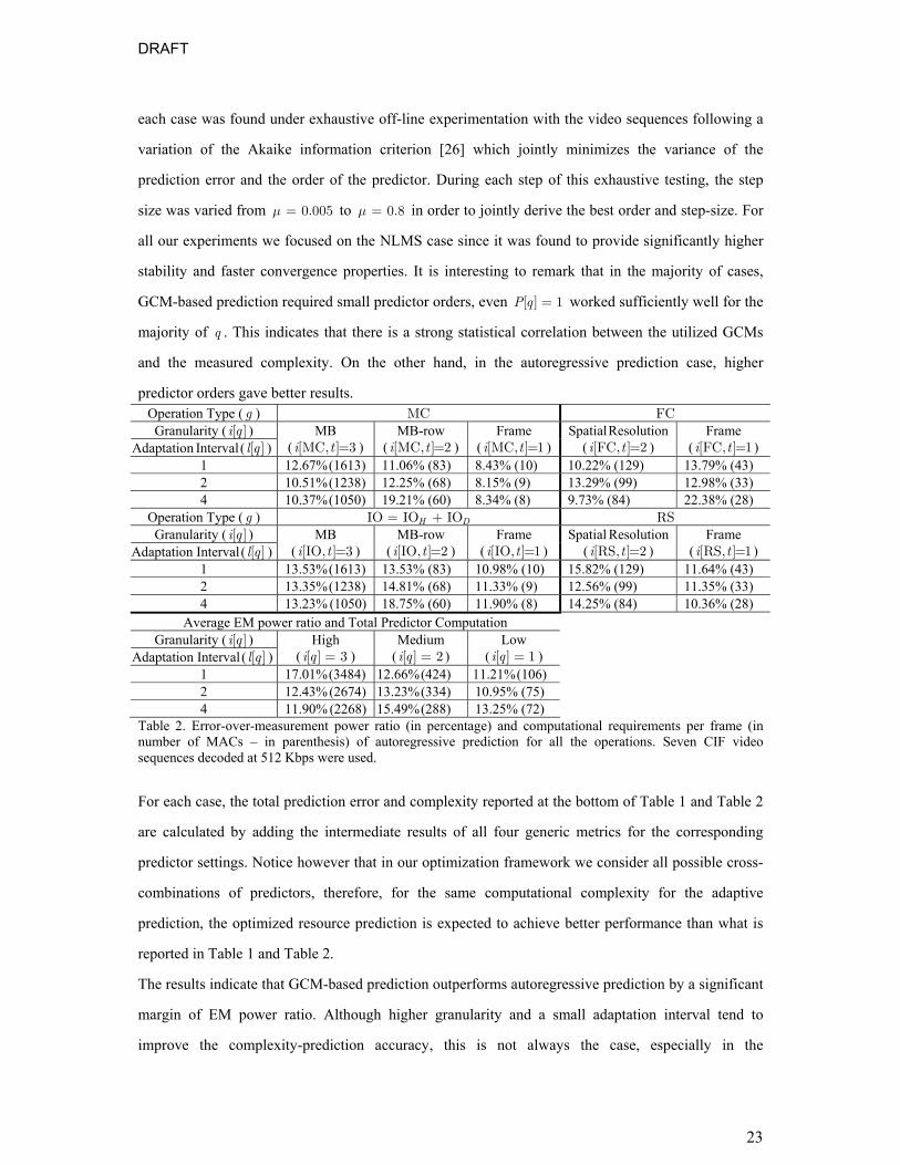
number of future frames whose complexity can be predicted is decreased. Operation Type ( g ) MC FC Granularity ( [ ]i q )

Adaptation Interval ( [ ]l q ) MB

( [MC, ]=3i t ) MB-row

( [MC, ]=2i t ) Frame

( [MC, ]=1i t ) Spatial Resolution

( [FC, ]=2i t ) Frame

( [FC, ]=1i t ) 1 4.07% (188) 4.58% (38) 5.82% (10) 8.56% (15) 9.19% (15) 2 3.47% (169) 3.90% (34) 5.40% (9) 9.17% (14) 10.22% (14) 4 4.45% (160) 6.47% (32) 6.16% (8) 10.22% (13) 14.98% (13)

Operation Type ( g ) IO IO IOH D= + RS Granularity ( [ ]i q )


( [IO, ]=3i t ) MB-row

( [IO, ]=2i t ) Frame

( [IO, ]=1i t ) Spatial Resolution

( [RS, ]=2i t ) Frame

( [RS, ]=1i t ) 1 3.70% (188) 4.69% (38) 5.71% (10) 8.86% (15) 8.04% (15) 2 3.40% (169) 4.52% (34) 6.40% (9) 6.77% (14) 9.41% (14) 4 5.56% (160) 13.51% (32) 6.50% (8) 10.84% (13) 8.25% (13)

Average EM power ratio and Total Predictor Computation Granularity ( [ ]i q )

Adaptation Interval ( [ ]l q ) High

( [ ] 3i q = ) Medium

( [ ] 2i q = ) Low

( [ ] 1i q = ) 1 6.29% (406) 6.67% (106) 7.19% (50) 2 5.70% (366) 6.09% (96) 7.86% (46) 4 7.77% (346) 10.26% (90) 8.97% (42)

Table 1. Error-over-measurement power ratio (in percentage) and computational requirements per frame (in number of MACs – in parenthesis) of GCM-based prediction for all the different operations. Seven CIF video sequences decoded at 512 Kbps were used.

Different sampling granularities are considered in the experiments reported in Table 1 and Table 2, as

explained in Subsection III.B. In addition, we considered different predictor adaptation intervals. The

reported experiments used the best predictor order not greater than 64. The best predictor order for

DRAFT

23

each case was found under exhaustive off-line experimentation with the video sequences following a

variation of the Akaike information criterion [26] which jointly minimizes the variance of the

prediction error and the order of the predictor. During each step of this exhaustive testing, the step

size was varied from 0.005µ = to 0.8µ = in order to jointly derive the best order and step-size. For

all our experiments we focused on the NLMS case since it was found to provide significantly higher

stability and faster convergence properties. It is interesting to remark that in the majority of cases,

GCM-based prediction required small predictor orders, even [ ] 1P q = worked sufficiently well for the

majority of q . This indicates that there is a strong statistical correlation between the utilized GCMs

and the measured complexity. On the other hand, in the autoregressive prediction case, higher

predictor orders gave better results. Operation Type ( g ) MC FC Granularity ( [ ]i q )


( [MC, ]=3i t ) MB-row

( [MC, ]=2i t ) Frame

( [MC, ]=1i t ) Spatial Resolution

( [FC, ]=2i t ) Frame

( [FC, ]=1i t ) 1 12.67% (1613) 11.06% (83) 8.43% (10) 10.22% (129) 13.79% (43) 2 10.51% (1238) 12.25% (68) 8.15% (9) 13.29% (99) 12.98% (33) 4 10.37% (1050) 19.21% (60) 8.34% (8) 9.73% (84) 22.38% (28)

Operation Type ( g ) IO IO IOH D= + RS Granularity ( [ ]i q )


( [IO, ]=3i t ) MB-row

( [IO, ]=2i t ) Frame

( [IO, ]=1i t ) Spatial Resolution

( [RS, ]=2i t ) Frame

( [RS, ]=1i t ) 1 13.53% (1613) 13.53% (83) 10.98% (10) 15.82% (129) 11.64% (43) 2 13.35% (1238) 14.81% (68) 11.33% (9) 12.56% (99) 11.35% (33) 4 13.23% (1050) 18.75% (60) 11.90% (8) 14.25% (84) 10.36% (28)

Average EM power ratio and Total Predictor Computation Granularity ( [ ]i q )

Adaptation Interval ( [ ]l q ) High

( [ ] 3i q = ) Medium

( [ ] 2i q = ) Low

( [ ] 1i q = ) 1 17.01% (3484) 12.66% (424) 11.21% (106) 2 12.43% (2674) 13.23% (334) 10.95% (75) 4 11.90% (2268) 15.49% (288) 13.25% (72)

Table 2. Error-over-measurement power ratio (in percentage) and computational requirements per frame (in number of MACs – in parenthesis) of autoregressive prediction for all the operations. Seven CIF video sequences decoded at 512 Kbps were used.

For each case, the total prediction error and complexity reported at the bottom of Table 1 and Table 2

are calculated by adding the intermediate results of all four generic metrics for the corresponding

predictor settings. Notice however that in our optimization framework we consider all possible cross-

combinations of predictors, therefore, for the same computational complexity for the adaptive

prediction, the optimized resource prediction is expected to achieve better performance than what is

reported in Table 1 and Table 2.

The results indicate that GCM-based prediction outperforms autoregressive prediction by a significant

margin of EM power ratio. Although higher granularity and a small adaptation interval tend to

improve the complexity-prediction accuracy, this is not always the case, especially in the

DRAFT

24

0 50 100 150 200 2500

500

1000

1500

2000

2500

3000

3500

4000

4500

5000

Entropy Decoding: 'Tempete', 1536000kbps; Adaptation at Spatial-resolution Granularity AND Prediction at Frame Granularity

Tics

Decoded MCTF frame #

measurementGCM-based predictionAutoregressive prediction

0 50 100 150 200 250 300 350 400 450 5000

500

1000

1500

2000

2500

3000

3500

4000

4500

5000

Motion Compensation: 'Tempete', 1536000kbps; Adaptation AND Prediction at Frame granularity

Tics

Predict or Update Step #


0 50 100 150 200 2500

500

1000

1500

2000

2500

3000

3500

4000

4500

5000

Entropy Decoding: 'Tempete', 1536000kbps; Adaptation AND Prediction at Frame Granularity

Tics

Decoded MCTF frame #


0 50 100 150 200 250 300 350 400 450 5000

500

1000

1500

2000

2500

3000

3500

4000

4500

5000

Motion Compensation: 'Tempete', 1536000kbps; Adaptation at MB granularity AND Prediction at Frame Granularity

Tics

Predict or Update Step #


autoregressive prediction case. For example, for the GCM-based prediction of MC operations, the

best result is obtained under an adaptation interval of 2 measurements at the macroblock granularity.

This means that other combinations with higher complexity and higher expected error should be

excluded. This is automatically performed during the off-line pruning process of the proposed

optimization framework, as described in the previous section. Consequently, it can be said that the

proposed off-line optimization framework automatically provides the subset of predictor

configurations that always provide lower (expected) error for higher complexity without incurring any

additional on-line computation penalty.

Figure 5. Examples of GCM-based and autoregressive-based execution time prediction. The time required for the motion compensation and entropy decoding operations for the reconstruction of all MCTF frames of each GOP of one video sequence are presented. Top row: Predictor adaptation with macroblock or spatial-decomposition level granularity; bottom row: predictor adaptation with frame granularity. “Tics” indicate the value measured by the internal processor counter and the prediction error is always measured in a frame-by-frame basis.

Examples of GCM-based and autoregressive complexity prediction across time are given in Figure 5

where we report the prediction estimates versus the time measured in units (“tics”) of the internal

processor counter [25]. As shown in the figure, the autoregressive-based prediction tends to

“overshoot” or “undershoot” during the complexity estimation in comparison to the GCM-based

DRAFT

25

prediction that appears to follow the experimental results more accurately. An additional aspect of the

GCM-based approach is that the prediction with a higher granularity (i.e. at the macroblock or spatial-

decomposition level) tends to follow the actual measurements with significantly higher accuracy than

that at the decoded frame granularity even though the two methods may happen to be comparable

when the prediction is averaged over a time interval (e.g. corresponding to a GOP). This is not

necessarily true for autoregressive complexity prediction as shown by the relevant experiments in

Figure 5. Notice though that GCM-based prediction also requires communication overhead for the

transmission of the GCM values, or the modeling parameters via which GCMs may be derived [17].

The communication overhead is proportional to the granularity and the adaptation interval at which

complexity is predicted (see (20)). Hence the proposed optimization framework that operates with

bounded predictor complexity implicitly bounds the communication overhead for the GCM

transmission to the receiver as well.

IV.B. Resource-constrained Complexity Prediction

The results of Table 1 and Table 2 demonstrate that GCM-based prediction is significantly

better than autoregressive prediction and requires on average less complexity for the predictor

realization, we focus on this category for the remainder of this section. For the optimization

framework of Section III the process is performed as follows:

IV.B.1 Algorithm Summary

• We apply the off-line bootstrapping process of Subsection III.E to the seven video sequences used

previously for the estimation of the expected error for each predictor configuration under the ten

confidence intervals mentioned in Subsection III.E.

• The off-line pruning process of Subsection III.D is subsequently applied for each confidence

interval. All the admitted predictor configurations from the explored parameter space of Figure 3

are then sorted (off-line) in decreasing complexity (and hence increased estimation error). In this

way, for each temporal level we obtain estimations of predictor complexity and expected error such

as the ones seen in Figure 6. The results of the figure were generated with two confidence intervals

for the bootstrap process. Similar results were obtained with other confidence intervals, and for the

remaining temporal levels.

• During the on-line complexity estimation, we use (14), (15) and for every temporal level t we have

( , ) [ , ] [ , ] [ , ] [ , ]( ) ( )g t i g t i g t i g t i g tu n p g n p− = − and [ , ] 0i g tk = for the GCM-based prediction. The

DRAFT

26

complexity predictor parameters [ ]i q and [ ]l q are obtained by the given predictor complexity bound

bound 1O ( )n and the current confidence parameter [ ]qε based on the off-line sorted list of admitted

predictor configurations from the previous step.

0 200 400 600 800 1000 1200 1400 1600 1800 20000

100

200

300

400

500

600

700

800

900GCM-based Predictor Complexity - All generic operations, Temporal level 2

Predictor Configuration Number

MA

C o

pera

tions

per

dec

oded

fram

e

0 200 400 600 800 1000 1200 1400 1600 1800 20000.1

0.2

0.3

0.4

0.5

0.6

0.7

0.8

0.9

1Normalized Prediction Error - All generic operations, Temporal level 2


(Boo

tstra

p E

rror P

ower

) / (M

easu

rem

ent P

ower

)

0 500 1000 1500 2000 2500 3000 3500 40000

100

200

300

400

500

600

700

800

900GCM-based Predictor Complexity - All generic operations, Temporal level 2


MA

C o

pera

tions

per

dec

oded

fram

e

0 500 1000 1500 2000 2500 3000 3500 40000.1

0.2

0.3

0.4

0.5

0.6

0.7

0.8

0.9

1Normalized Prediction Error - All generic operations, Temporal level 2


(Boo

tstra

p E

rror P

ower

) / (M

easu

rem

ent P

ower

)

Figure 6. Complexity and bootstrap error of the GCM-based prediction for the case of temporal level two. Top: confidence interval : [ ,2] 1.0g gε∀ = ; bottom: confidence interval : [ ,2] 0.5g gε∀ = . Each predictor configuration number corresponds to a particular setting for the predictor order, predictor adaptation period and granularity of the application of the predictor from the parameter space of Figure 3.

IV.B.2 Experimental Results

Since only the last step from the above is performed on-line, the on-line complexity prediction

is guaranteed to have complexity equal to bound 1O ( )n . Table 3 presents the overall complexity-

prediction error for different predictor complexity bounds based on the optimization of (25) for four

sequences (“Coastguard”, “Paris”, “News”, “Stefan”) not belonging to the training set for the

bootstrap estimation process. Similar to our previous experiments, the prediction error was measured

for each decoded frame and a prediction interval of one GOP was selected. We begin the prediction

with confidence interval corresponding to [ ] 1.0qε = q∀ ∈ Q , and for each consecutive GOP we adapt

DRAFT

27

the confidence parameter [ ]qε (parameter for each operation and each temporal level) to the one which

produces the closest prediction to the observed errors. During our experimentation we observed that,

depending on the sequence characteristics and the mismatch between the off-line estimated error and

the actual prediction error, frequent changes in the predictor configuration may occur. This is not

desirable since additional error is caused until the new predictor converges to the (quasi) steady state.

Hence, to indicate the penalization cause by the new predictor convergence time, we included a bias

for the error estimate of the current predictor configuration by scaling it down by a certain percentage.

The best scaling value was determined experimentally.

IV.B.3 Practical Complexity and Communication Overhead for GCM-based Adaptive Complexity

Prediction

Due to the fact that we are performing software-only decoding simulations and the utilized

codec does not support real-time decoding under the chosen experimental setting, it is hard to

explicitly quantify the real effect of the complexity predictor versus the entire decoder complexity.

However, considering that one of the most complex modules of the decoder is the inverse spatial

transform, which by itself can operate in real-time in our decoder, preliminary results indicate that the

most complex instantiation of the predictor used in the results of Table 3 and tested as a software-only

C++ module, required approximately 25% of the execution time of the inverse transform. This

complexity is substantially reduced as the bound on the predictor MAC operations is decreased. In

addition, further optimization of both the decoder or the complexity predictor implementation may

change the relative complexity overhead added into the overall decoding process. Hence, the practical

quantification of this overhead in a real-time environment remains a future research topic.

Finally, concerning the transmission overhead for the communication of the GCM values to the

decoder, in all the experiments reported in Table 3, the overhead was ranging from 0.5% to no more

than 8% of the overall transmission bitrate. Since there is a linear relationship between (18) and (20)

(complexity and information requirements of GCM-based prediction), the higher the bound set for

bound 1O ( )n , the more the GCM transmission overhead.

bound 1O ( )n (in MAC operations per decoded frame of each GOP) 500 200 50

Average 2

out 1 out 1( ) ( )e c n n (256 Kbps) 2.88% 5.74% 7.45%

Average 2

out 1 out 1( ) ( )e c n n (512 Kbps) 3.77% 4.44% 6.91%

Average 2

out 1 out 1( ) ( )e c n n (1024 Kbps) 3.11% 4.82% 7.21%

Table 3. Results of resource-constrained complexity prediction. Prediction was applied for the decoding complexity of each subsequent GOP of the sequence and the prediction error is measured per video frame.

DRAFT

28

V. DISCUSSION The results of the statistical estimation of the expected error versus the predictor complexity

shown in Figure 6 serve as a validation that the proposed GCM-based complexity prediction approach

provides lower resource-prediction error for increased computation bound for the predictor. This was

additionally tested in practice with new sequences as demonstrated by the results of Table 3. The

monotonic relationship between predictor complexity and expected prediction error is a significant

aspect of the proposed framework since, in this way, depending on the delay deadline for the

decoding of each GOP, one can assign appropriate complexity to the resource prediction such that

sufficient prediction accuracy is obtained for the particular application. The proposed framework

appears to be able to provide good complexity estimates over a variety of sequences and bitrates, even

though all the off-line training steps and the on-line adaptation are essentially agnostic to the specific

decoding operations and their implementation details. In fact, even though the estimation experiments

for Table 3 were performed under a slightly different processor and under different processor load

(which is anyway not constant in the Windows XP operating system) in comparison to our training

stage, the on-line adaptation of the confidence interval for the bootstrap error estimates appears to

cope well with these effects.

The proposed complexity-prediction framework can be used in several cases where delay-bounded

video decoding is to be performed at a receiver. For example, under the flexible video decoding

model [19], the proposed adaptive prediction can be used to accurately estimate the remaining time

for each frame of each GOP. These estimates can be communicated to the operating system which can

decide to increase or decrease the resources allocated to the particular task [29] [30] [31] as long as

the delay deadline is not violated.

Another application of the proposed complexity-prediction framework is in admission control for a

video bitstream to be decoded by a particular system. As shown in our previous work [17], the

complexity mapping can generate bounds on each of the possible operations (MC , IOH , IOD , FC

and RS ) and request that these bounds be satisfied for each GOP of the decoded video sequence. This

effectively creates a dynamic complexity-specification (C-SPEC) negotiation mechanism between the

video server and each client decoder that implements the complexity prediction. Although we have

presented some preliminary results of such a negotiation in our previous work [17] [18], we plan to

investigate this issue further in our future research.

DRAFT

29

VI. CONCLUSIONS Accurate and generic methods for video-decoding resource prediction can provide significant

improvements for scheduling and resource optimization algorithms in multimedia platforms. This

paper analyzed in a systematic manner the various alternatives involved in autoregressive linear

prediction or prediction based on generic complexity metrics. Our analysis led to the definition of an

off-line estimation process for resource-constrained complexity prediction followed by on-line

adaptation of the prediction parameters. A large parameter space was taken into consideration. Our

results indicated that the GCM-based approach provides better resource-prediction accuracy with

lower computational requirements for the adaptive predictor. Moreover, under the proposed

optimization approach, the resource-prediction accuracy is gracefully improved with increased

predictor complexity, thereby providing an adaptable framework useful for a variety of applications

involving resource optimization for multimedia decoding.

REFERENCES [1] M. Horowitz, A. Joch, F. Kossentini and A. Hallapuro, “H.264/AVC baseline profile decoder complexity

analysis,” IEEE Trans. Circuits and Syst. for Video Technol., vol. 13, no. 7, pp. 704-716, July 2003. [2] V. Lappalainen, A. Hallapuro and D. Hamalainen, “Complexity of Optimized H.26L video decoder

implementation,” IEEE Trans. Circuits, Syst. for Video Technol., vol. 13, no. 7, pp. 717-725, July 2003. [3] J. Valentim, P. Nunes and F. Pereira, “Evaluating MPEG-4 video decoding complexity for an alternative

video complexity verifier model,” IEEE Trans. Circuits and Syst. for Video Technol., vol. 12, no. 11, pp. 1034-1044, Nov. 2002.

[4] S. Saponara, C. Blanch, K. Denolf and J. Bormans, “The JVT advanced video coding standard: complexity and performance analysis on a tool-by-tool basis,” Proc. Packet Video Workshop, (PVC), pp., April 2003.

[5] M. Ravasi and M. Mattavelli, “High-abstraction level complexity analysis and memory architecture simulations of multimedia algorithms,” IEEE Trans. Circuits and Syst. for Video Technol., vol. 15, no. 5, pp. 673-684, May 2005.

[6] M. Ravasi and M. Mattavelli, “High-level algorithmic complexity evaluation for system design,” Journal of Systems Architecture, vol. 48, pp. 403-427, 2003.

[7] A. C. Bavier, A. B. Montz and L. Peterson, “Predicting MPEG execution times,” Proc. ACM SIGMETRICS, pp. 131-140, 1998.

[8] P. A. Dinda, and D. R. O’Hallaron, “An evaluation of linear models for host load prediction,” Proc. IEEE Internat. Sympos. High Perf. Distrib. Comput., pp. 87-96, Aug. 1999.

[9] W. Yuan and K. Nahrstedt, “Energy-efficient CPU scheduling for multimedia applications,” ACM Trans. on Computer Syst., vol. , no. , 2006.

[10] J. Liang, K. Nahrstedt, and Y. Zhou, “Adaptive multi-resource prediction in distributed resource sharing environment,” Proc. IEEE Internat. Sympos. On Cluster Comput. and the Grid, CCGrid-04, pp. 293-300,April 2004.

[11] D. G. Sachs, S. V. Adve and D. L. Jones, “Cross-layer adaptive coding to reduce energy on general-purpose processors,” Proc. IEEE Internat. Conf. on Image Process., vol. 3, pp. 109-112, Sept. 2003.

[12] H. J. Stolberg, M. Berekovic, and P. Pirsch, “A platform-independent methodology for performance estimation of streaming media applications,” Proc. IEEE Internat. Conf. on Multimedia and Expo, (ICME), vol. 2, pp. 105-108, Aug. 2002.

[13] H. J. Stolberg, M. Berekovic, and P. Pirsch, “A platform-independent methodology for performance estimation of multimedia signal processing applications,” Journal of VLSI Signal Process., vol. 41, pp. 139-151, 2005.

DRAFT

30

[14] Z. He, Y. Liang, L. Chen, I. Ahmad and D. Wu, “Power-rate-distortion analysis for wireless video communication under energy constraints,” IEEE Trans. Circuits and Syst. for Video Technol., vol. 15, no. 5, pp. 645-658, May 2005.

[15] M. Mattavelli and S. Brunetton, “Implementing real-time video decoding on multimedia processors by complexity prediction techniques,” IEEE Trans. on Cons. Electronics, vol.44, no.3, pp.760-767, Aug.1998.

[16] G. Landge, M. van der Schaar and V. Akella, “Complexity metric driven energy optimization framework for implementing MPEG-21 scalable video decoders,” IEEE Internat. Conf. Accoust., Speech, and Sig. Proc., vol. 2, pp. 1141-1144, March 2005.

[17] Y. Andreopoulos and M. van der Schaar, "Complexity-constrained video bitstream shaping," IEEE Trans. on Signal Processing, to appear.

[18] M. van der Schaar and Y. Andreopoulos, "Rate-distortion-complexity modeling for network and receiver aware adaptation," IEEE Trans. on Multimedia, vol. 7, no. 3, pp. 471-479, June 2005.

[19] S. Regunathan, P. A. Chou and J. Ribas-Corbera, "A generalized video complexity verifier for flexible decoding," IEEE International Conference on Image Processing, (ICIP), vol. 3, pp. 289-292, Sept. 2003.

[20] M. T. Sun and A. R. Reibman (eds), Compressed video over networks, New-York: Marcel Dekker, 2001. [21] T. Wiegand, G. Sullivan, G. Bjontegaard, and A. Luthra, “Overview of the H.264/AVC video coding

standard,” IEEE Trans. on Circuits and Syst. for Video Technol., vol. 13, no. 7, July 2003. [22] J. R. Ohm, M. van der Schaar and J. W. Woods, “Interframe wavelet coding – Motion picture

representation for universal scalability,” Signal Processing: Image Communication, vol 19. no. 9, pp. 877-908, Oct. 2004.

[23] H. Schwarz, T. Hinz, H. Kirchhoffer, D. Marpe, and T. Wiegand, “Technical description of the HHI proposal for SVC CE1,” ISO/IEC JTC1/SC29/WG11 (MPEG), m11244, Oct. 2004.

[24] Y. Andreopoulos, A. Munteanu, J. Barbarien, M. van der Schaar, J. Cornelis and P. Schelkens, "In-band motion compensated temporal filtering," Signal Process.: Image Commun. (special issue on "Subband/Wavelet Interframe Video Coding"), vol. 19, no. 7, pp. 653-673, Aug. 2004.

[25] Intel Corp. “Intel ® VTune ™ data collector enabling kit for I/O Processors”, Application Note 273892-001, available on-line at: http://developer.intel.com/design/iio/applnots/27389201.pdf

[26] S. Haykin, Adaptive filter theory, Engewood Cliffs, NJ: Prentice Hall, 1991. [27] B. Hassibi, A. H. Sayed and T. Kailath, “H∞ optimality of the LMS algorithm,” IEEE Trans. on Signal

Process., vol. 44, no. 2, pp. 267-282, Feb. 1996. [28] A. M. Zoubir and B. Boashash, “The bootstrap and its application in signal processing,” IEEE Signal

Process. Mag., pp. 56-76, Jan. 1998. [29] M. Srivastava, A. Chandrakasan and R. Brodersen, “Predictive system shutdown and other architectural

techniques for energy efficient programmable computation,” IEEE Trans. on Very Large Scale Integrat., vol. 4, no. 1, pp. 42-55, March 1996.

[30] S. Irani, G. Singh, S. K. Shukla and R. K. Gupta, “An overview of the competitive and adversarial approaches to designing dynamic power management strategies,” IEEE Trans. on Very Large Scale Integrat., vol. 13, no. 12, pp. 1349-1362, Dec. 2005.

[31] W. Yuan, K. Nahrstedt, S. V. Adve, D. L. Jones and R. H. Kravets, “GRACE: Cross-layer adaptation for multimedia quality and battery life,” IEEE Trans. on Mobile Comput., vol., no. 2006.

Yiannis Andreopoulos and Mihaela van der Schaar...

Documents

Transcript of Yiannis Andreopoulos and Mihaela van der Schaar...