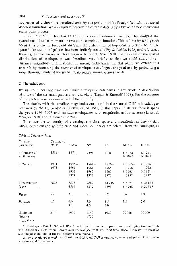
Geophys. J. R. astr. SOC. (1980) 62, 303-320.

Spatial distribution of earthquakes: the two-point correlation function

Y. Y. Kagan and L. Knopoff Institute of Geoplzysics and Planetary Physics, G'niversity o,f California, Los Arigeles, USA

Received 1979 November 13;in original form 1979 January 29

Summary. The distribution of distances between pairs of earthquake epicentres and hypocentrks has been determined for four local and two world-wide catalogues. These spatid correlation functions shows that the number of events per unit volume at distance R from any earthquake is proportional to R - q where ct is close to 1.0 for shallow earthquakes and increases to 1.5 or possibly larger for deeper events. This distribution of earthquakes is independent of magnitude and independent of the dimensions of the region under consideration. These results place limits on possible models of earthquake fault geometries.

1 Introduction

The study of the spatial distribution of earthquakes is of particular importance to several branches of seismology including seismic risk analysis and source mechanism theory. A knowledge of the geometry of faulting may enhance our ability to predict future seismic activity in a given area and to compare seismic data with geologic or geodetic information. With regard to source theory, the geometry of dynamical rupture places constraints on the nature of the source wave form. These two problems may be related (Kagan & Knopoff 1980) by virtue of the self-similarity of the earthquakes process: a single earthquake can be considered as a model, or rather an automodel, of a sequence of earthquakes, each with a suitable change of time and distance scales, a topic we will pursue elsewhere.

A first approximation to the geometry of faulting is that of an earthquake as an infini- tesimal plane dislocation. Earthquake faults in nature are much more complex; they bend, branch and merge. Such phenomena occur on the scale of dynamical fracture of individual earthquakes as well. In this paper we describe the geometry of an ensemble of earthquakes quantitatively to see if any systematic changes in these descriptions occur on different scales of distance. We make the postulate that any systematic behaviour we uncover can be extended to faults on the scale of individual events.

One limitation on developing such a description is the availability of data. Information about the distribution of earthquakes that is readily accessible at present does not include moment tensor data, but instead is restricted to earthquake catalogues where the spatial

304 Y. Y. Kagan and L. Knopoff

properties of a shock are described only by the position of its focus, often without useful depth information. An appropriate description of these data is by a two- or three-dimensional scalar point process.

Since none of the foci has an absolute frame of reference, we begin by studying the spatial second-order moment or two-point correlation function. This is done by taking each focus as a centre in turn, and analysing the distribution of hypocentres relative to it. The spatial distribution of galaxies has been similarly treated (Fry & Peebles 1978, and references therein). In two earlier articles (Kagan & Knopoff 1976, 1978) the problem of the spatial distribution of earthquakes was described very briefly so that we could study time- distance-magnitude interrelationships among earthquakes. In this paper we extend this research by increasing the number of earthquake catalogues analysed and by performing a more thorough study of the spatial relationships among various events.

2 The catalogues

We use four local and two world-wide earthquake catalogues in this work. A description of three of the six catalogues is given elsewhere (Kagan & Knopoff 1978). For the purpose of completeness we summarize all of them briefly.

The shocks with the smallest magnitudes are found in the Central California catalogue prepared by the US Geological Survey, called USGS in this paper. In its raw form it spans the years 1969-1975 and includes earthquakes with magnitudes as low as zero (Lester & Meagher 1978, and references therein).

To ensure the uniformity of a catalogue in time, space and magnitude, all earthquakes which occur outside specific time and space boundaries are deleted from the catalogue, as

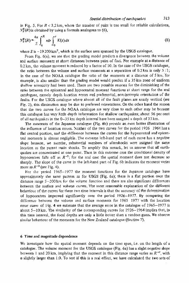
Table 1. Catalogue data.

Catalogue Catalogues parameters USCS CACA

n (number of 5586 837 earthquakes

Time (yr) 1971- 1944- 1975 1961

1962- 1974

Time intervals 1826 6575 (day) 4564

Mmax 5.2 7.1

Mcut-off 1.5 4.0 3.5

Maximum 378 1000 distance Rmax (km)

NZ

1396

1940- 1966 1967- 1977

9862 3872

7.1

5 .O 4.5

1340 1720

JP

1025

1926- 1964

1977

14 245 4595

8.2

5.5 5 .O

1920

1965-

NOAA

a. 4982 b. 7885

a. 1965- 1976

b. 1965- 1977

a. 4077 b.4748

8.6

5.3

20 000

DUDA

a. 1271 b. 1070

a. 1905- 1972

1977

a. 24 838 b. 20 819

8.9

7.0

b. 1921-

20 000

1. Catalogues CACA, NZ and J P are each divided into two separate non-overlapping time intervals with different cut-off magnitudes in each interval (see text). The total time interval from start to finish of a catalogue is the sum of the two separate time intervals.

2. Two overlapping versions of both the NOAA and DUDA catalogues were used and are identified as versions a and b (see teyt).

Spatial distribution of earthquakes 305

well as all earthquakes with magnitudes less than some cut-off limit (Kagan & Knopoff 1978). These bounds are dependent on the locations of the seismographic stations; the lower magnitude cut-off was determined from an analysis of magnitude-frequency relations. As a result of this truncation, 90 per cent or more of the USGS catalogue in its original form was rejected. A brief summary of the data used in this paper is presented in Table 1 ; the geographical boundaries used to delimit this and the other California catalogues are shown in Figs 1 and 2(a).

The California catalogue (CACA) was compiled from a fusion of the Northern California and Southern California catalogues. Because of changes in the density and quality of the networks in the early 1960s, two lower magnitude cut-offs were applied to the data: ML =4.0 for the period 1944-1961, and M L = 3.5 thereafter (Kagan & Knopoff 1978).

The New Zealand catalogue (NZ) was taken from the compilation by Smith (1976). All earthquakes prior to 1940, as well as shocks outside New Zealand proper, were deleted. The boundaries of the region form a rectangle with comers (34" S, 175" E), (39" S, 180" E), (46" S, 173" E), (41" S, 168" E). Subsequent to 1967 January 1, the southern and western corners of the region were moved to (49" S, 170" E) and (44" S, 16.5" E).

The Japanese catalogue (JP) has been taken from data prepared by the Japan Neteoro- logical Agency (1958, 1966, 1968). The region is defined by the pentagon with corners

Figure Central

306

(46"N, 142"E), (44"N, 146"E), (35"N, 141"E), (31"N, 131"E)and (33.4"N, 129.4"E). Only shallow earthquakes were used; the magnitude cut-off was 5.5 for the period 1926- 1964 and 5.0 for 1965-1977.

The two world-wide catalogues were the DUDA catalogue which is an updated version of that given by Duda (1965) and the NOAA catalogue which is based on the Preliminary Determination of Epicenters (PDE). The major changes we have introduced in this latter catalogue, beyond the elimination of weak shocks as described above, was to recalculate and average the magnitudes to correct for the saturation of the mb and M s scales for strong earthquakes (Kagan & Knopoff 1980). Most of our results for the NOAA catalogue in this paper were based on the listing of earthquakes of 1965-1976. Figs 9(a) and 11 were based on earthquakes from 1965-1977 (see Table 1 ) . Fig. 9(b) also makes use of the DUDA catalogue as updated by B l t h & Duda ( I 979).

Y. Y. Kagan and L. Knopoff

3 Epicentral second-order moment

At first glance it would seem to be rather easy to describe a set of earthquake hypocentres (or epicentres) such as those illustrated in Figs 1 and 3. Many earthquakes are associated with known faults or faults inferred from the same catalogue data. A comparison of Figs 1

39

38

3 7

3 6

35

-123 -122 -121 -120

Figure 2. (a, b, c) Seismicity maps for USGS region (1971-1975).

'

-122.00 -121.75

X .

X

. * * .

2 -

I. . f * f . * .

0

P

31. 00

36.75

3 6 . 5 0

3 6 . 2 5

36.00

-121.50 - 1 21.25 -121.00

36.75

36.70

36.65

36.55

36.50

307

-121.25 -121.20 -121.15 -121.1C -121.05 -121.00

308

and 2(a) shows the important role of errors in location of epicentres; these errors are of the order of 5 km for the CACA catalogue and 0.5-1.Okm for the USGS catalogue. In Fig. 1 the epicentres inside the boundaries of USGS form a rather diffuse cloud, whereas in Fig. 2(a) they are concentrated along several well-known faults including the San Andreas, Sargent, Calaveras and Haywards faults from south to north. If we expand the picture (Fig. 2b, c) the set of epicentres once again loses its well-defined features. This may be due to location errors, to the non-verticality of faults on which earthquakes occur, or to the possibility that some earthquakes occur on faults that are ill-defined due to low seismicity. A comparison of all four maps shows a certain similarity, as though the change of scale does not alter the basic pattern of the spatial earthquake distribution. We propose that this spatial scale- independence or self-similarity is a major feature of seismicity; most of this paper is concerned with a quantitative exploration of this proposition.

A low-order statistical description of the data is given by its conditional spatial first-order moment function, which is the average number of shocks per unit surface area or volume that are situated at a certain distance from any given earthquake focus, in either two or three dimensions. The second-order moment m2(x2 , x,) is defined in terms of the conditional first-order moment ml(x2 Ix,) through the expression mz(x2 , x , )=mi (x l )m ](xZ I xl ) , where ml (x l ) is the ordinary first-order moment of the process (Cox & Lewis 1966);in our case ml(x ) is the spatial density of epicentres and hypocentres and x is the two- or three- dimensional vector of an earthquake focus.In practice, we define the unnormalized conditional first-order moment function as the number of pairs of earthquakes N2(R) or N,(R) for which the distances between epicentres or hypocentres are smaller than R respectively. The subscripts on N2 or N 3 indicate the dimensionality of the space. In principle the numbers N2 or N 3 should be normalized by dividing by the surface area SR or volume V , of a circle or sphere of radius R . Difficulties arise due to edge effects when our sampling circle or sphere lies partly outside the boundaries of the area or volume spanned by the catalogue; the volume effects may include those due to non-uniformity of the seismicity as a function of depth. To account for these effects as fully as possible, we divide N 2 ( R ) by the number of earthquake pairs N f ( R ) which would be obtained if the same number of earthquakes were randomly distributed throughout the whole area, i.e. according to a Poisson distribution. A similar normalization is made for N3(R) . This ratio therefore describes the difference between the actual spatial distribution of earthquakes and a Poisson distribution.

Fig. 3 shows the ratio N 2 ( R ) / N f ( R ) for four catalogues of shallow earthquakes with widely different spans of distances, magnitudes and location errors. For display purposes this ratio has been multiplied by R and divided by the maximum dimension of the region R,,,. We have shown the epicentral moment N 2 ( R ) normalized as above instead of the more physically natural hypocentral moment N , ( R ) because catalogues CACA, DUDA and NOAA either lack or have insufficiently detailed information about focal depths for shallow earth-

Y. Y. Kagan and L. Knopoff

l l . a ! __ ~i~~ , ! . c : 3 . c 10C.0 1000 .0 iooo0.o

;?s:;>LE N F

Figure 3. Spatial surface moments.

Spatial distribution of earthquakes 309

quakes. The curve for each catalogue exhibits a similar behaviour: a rise at short range, a rmearly flat middle portion and again a rising later part. We assume that the fact that the ratio in independent of distance in the middle part of the plot is a real physical effect. Most of the discussion in the remainder of this paper is the confirmation and elaboration of this observa- tion. As we show below, the shape of the curves is controlled mostly by location errors when R is small; when R is comparable with Rmm, geometrical factors other than those already mentioned begin to influence the shape of the curve.

4 Location and projection errors

To study the influence of uncertainties in location, let us make the assumption, for simpli- city, that the hypocentral location errors u are approximately equal in all three directions. Then the distribution of distance between two hypocentres whose actual separation is d, obeys a ‘non-central chi-distribution’ (Fisher 1928; Kendall & Moran 1963). It has three degrees of freedom; there are only two degrees of freedom for epicentres. The distribution density is

where all distances ir? formulae (1) and (2) have been normalized by dividing them by 61’2u, as for example

p = - .

The factor of 6 is the number of degrees of freedom of location of the two hypocentres. If, as suggested by the central part of the curves in Fig. 3, we assume that the spatial

moment is proportional to 1/R, we can compute the ratio RN,(R)/VR for the case for which all hypocentres are randomly, independently and isotropically shifted by an error vector u. Up to a constant of proportionality this is

d

u&

0

c

CL

- a

DISTANCE RATIO 0.01 0.10 1 .oo 10.00

1 .oo

0.50

0.20

0.10

0.05

0.02

0 .01 0

0 LOCATION ERROR MODEL

o GRADING MODEL

A SEISMICITY RESTRICTED TO DIAMETER OF CIRCLE + SEISMICITY RESTRICTED TO GREAT CIRCLE OF SPHERE

.001 0.010 0.100 1 .oo DISTANCE RRTIO. R I D

Figure 4. Theoretical spatial moments. The upper scale refers to the curves plotted with open symbols; the abscissas are R / ( 6 ” 2 0 ) and R/I. (see formulae 2 and 3) for the location error and grading models respectively. The lower scale is for the other two models defined by formulae (4) and (5). The lines to the right indicate the slope of spatial moments with Ro, R-’ and R-’ dcpendence.

310

This ratio is shown in Fig. 4. As might have been expected for distances R g 1, this ratio is proportional to Ro, which means that the hypocentres are uniformly distributed in space; for R > 1, this ratio approaches I/R, as expected.

Another possible source of distortion in the curves of Fig. 3 is the use of epicentral projections to locate earthquake foci. Errors in assigning focal depths contribute to statis- tical fluctuations in these projections. In some cases the errors in focal depth arise because the depth of focus is fixed, based on an a priori assumption regarding the depth distribution of seismicity; often the depth is rounded off in discrete steps such as 1 or 1Okm; for our purposes both of these models amount to the same result, which is a partial or complete loss of depth information. The process of projection of a three-dimensional distribution into a two-dimensional space is called 'grading' after Matheron (1971).

For illustrative purposes we have calculated the two-dimensional spatial moment, assum- ing that the original seismicity was isotropic and that the three-dimensional moment is proportional to 1/R. Then a horizontal layer of seismicity of thickness L is removed, and projected on a horizontal plane. The assumption of isotropy is difficult to justify, since an inspection of the maps of seismicity (Figs 1 and 2) shows that seismicity is locally highly anisotropic. If, for example, all hypocentres were associated with vertical faults of equal vertical dimension, there would be no difference between the epicentral and hypocentral moments, since all hypocentres project on to straight lines, and hence both ratios would vary as R-' . On the other hand, if the faults are all horizontal, the difference between the two moments would be maximized: the hypocentral moment would continue to be proportional to I/R, whereas the epicentral moment would be independent of distance, i.e., proportional to Ro. This difference is expected because all epicentres plot in the same configuration as on the fault plane; thus the same conditional number of events in each case is divided by R3 for volume and R2 for surface moments.

Y. Y. Kagan and L. Knopoff

For the above-mentioned model our ratio is (Matheron 1968):

RN2(R)/(.rrR2) a ( 2 / R ) I R r d r s (L - 1 2 ) (r2 + hz)-1/2 dk = 0 0

(B3 - ~ 3 - 1) (3 1 A

W 3 ) . + A log - - (B + 1 ) - (B - 1) -- A A

where A=R/L, B = (Az t i )"2 . Fig. 4 shows this ratio plotted against the quantity A. For R < L , the epicentral moment should be proportional to Ro=R-' .R. Matheron (1968, p. 109) indicates that multiplication of a moment by R is a general feature of grading. For R s L , the grading effect disappears and both moments coincide.

We have considered above the special case for which the standard errors of hypocentral location are equal in all three directions. However, errors in assignments of depths are usually much larger than those for epicentres. A possible prescription for estimating the distortions in the spatial moment in this case could involve the calculation of the horizontal or twodimensional error, followed by the grading of the spatial moment thus derived, i.e. by performing the epicentral projection separately. We do not carry out these calculations here.

The right hand edges of the curves in Fig. 3 have the value 1 when R=R,,; however as R approaches R,,, the relative positions of the curves vary significantly, depending on the alignments of the major faults of the region and the shape of the polygon which defines the seismic region. The number of major lineaments in the area and other geometrical features also influence the behaviour of the moment. We avoid the general case, and calcu- late the expectation value of the ratio for the two simple symmetric cases instead. In the

Spatial distribution of earthquakes 31 1 fist case, the seismicity was assumed to be confined to a diameter D of a circle and was d e n compared with the case of epicentral points randomly distributed throughout the area of the circle. The ratio is (Hammersley 1950)

where A = R/D. This curve (Fig. 4) can be compared with the right-hand parts of the curves for the USGS and CACA catalogues (Fig. 3). Although they are similar to a degree, good agreement is not expected since we have not taken into account the orientation of the faults.

For comparison with the worldwide catalogue, we have calculated the moment (Fig. 4) which would be obtained were all the world's seismicity concentrated along a single great circle with total length 2 0 . The ratio is

where A = R/D. Although the curves for the NOAA catalogue and the great circle model are similar (Figs 3 and 4), there are differences between them; we attempt to explain these differences below.

5 Hypocentral two-point function

We correct the hypocentral moment for the non-uniformity of the depth distributions of seismicity. The most suitable catalogue for this purpose is USGS, where the accuracy of the

1, 2 ,

~

h

D I S T R I B U T I O N OF HYPOCENTERS

COVARIANCE FUNCTION OF HYPOCENTRAL DEPTHS

COVARIANCE FUNCTION OF UNIFORM LAYER

Figure 5. Depth dependence, USGS catalogue.

312

depth determination is of the order of 1 km (see below). The depth distribution of shocks in USGS is shown in Fig. 5 . We compute the epicentral moment, which would be obtained were all the earthquakes distributed according t o the depth distribution shown in Fig. 5, instead of uniformly along the z-axis as in equation (3). The conditional volume moment is again taken to be proportional to 1/R. Then

Y. Y. Kagan and L. Knopoff

2 R RN2(R)/(.rrR2) ER I0 rdr Lw K ( z ) (r2 + zZ)-l'' dz.

The depth covariance function K(z) (Fig. 5 ) is defined as

K(z) = (Ah)-' [ N(h, h + Ah)N(h + z , h + z + Ah)dh (7)

where N(h, h + A h ) is the number of shocks in the depth interval (h,A t Ah). The covariance function is fairly well approximated by that for a layer 8 km in thickness

and having uniform seismicity (Fig. 5 ) . The grading curve calculated from equation 6 (Fig. 6a) is almost identical t o the grading model curve (Fig. 4) scaled by L = 8 km and hence the short range properties of the epicentral second-order moment are very likely due to grading effects. Thus, if the seismicity in the USGS catalogue were distributed uniformly and isotropically in a horizontal plane, the difference between the volume and surface moments could be estimated from these curves. The volume moment for this model would have a graph in Fig. 6 which is a horizontal line.

For distances greater than 3.2 km, the volume momentNf(R) tha t is needed to normalize the moment for the actual USGS catalogue is obtained simply by counting the number of pairs in a simulated Poissonian catalogue in which the same total number of points is distri- buted uniformly over a horizontal plane, and with depth distribution taken to be as shown

1 . o

0 . 5 0

0 .20

0 . 1 0

0 - 0 5

C.20

3 . 0 2

l l .01 s

t t 1

1 . c 1 6 . 0 ! O O .o 1003.0

DIST'NCE K"i

Figure 6 . Surface versus volume moiiientb ( a ) liS(;S and N O A 4 cataloeues. The grading model is calcu- la?ed for the LISGS catalogue. ( b ) Jt' catalopue. h G 70 k m .

Spatid distribution of earthquakes 313

in Fig. 5 . For R < 3.2 km, where the number of pairs i s too small for reliable calculations, .Vz(R)is obtained by using a formula andogous to (6),

where S is - 19 200 km', which is the surface area spanned by the USGS catalogue. From Fig. 6(a), we see that the grading model predicts a divergence between the volume

and surface moments at short distances between pairs of foci. For example at a distance of 0.2 km, the volume moment is reduced by a factor of 10. In the case of the USGS catalogue, the ratio between the volume and surface moments at a separation of 0.2km is only 5 : 1; in the case of the NOAA catalogue the ratio of the moments at a distance of 5 km, for example, is also smaller than the grading model would predict if a 35 km zone of uniform shallow seismicity had been used. There are two possible reasons for the diminishing of the ratio between the epicentral and hypocentral moment functions at short range for the real catalogues, namely depth location errors and preferential, nonisotropic orientation of the faults. For the USGS catalogue where almost all of the fault planes are nearly vertical (see Fig. 2), this diminution may be due to preferred orientations. On the other hand the reason that the two curves for the NOAA catalogue are very cIose t o each other may be because this catalogue has very little depth information for shallow earthquakes; about 56 per cent of a11 earthquakes in the 0-35 km depth interval have been assigned a depth of 33 krn.

The moments of the Japanese catalogue (Fig. 6b) provide an even better illustration of the influence of location errors. Neither of the two curves for the period 1926-1964 has a flat central portion, and the difference between the curves for the hypocentral and epicen- tral moments is almost negligible. The extreme left-hand part of each curve has a negative slope because, we surmise, substantial numbers of aftershocks were assigned the same location as the parent main shocks. To amplify this remark, let us assume that all earth- quakes are concentrated at one point. Then in this extreme case the conditional density of hypocentres falls off as R - 3 ; for the real case the spatial moment does not decrease so sharply. The slope of the curve in the left-hand part of Fig. 6b indicates the moment varies more as R-2 (see Fig. 4).

For the period 1965-1977 the moment functions for the Japanese catalogue have approximately the same pattern as for USGS (Fig. 6a); there is a flat portion over the distance range 5-200km for the volume function and there are also significant differences between the surface and volume curves. The most reasonable explanation of the different behaviour of the curves for these two time intervals is that the accuracy of the determination of hypocentres improved significantly over the period 1926-1977. By comparing the difference between the volume and surface moments for 1965-1977 with the location error curve of Fig. 4 we estimate that the average error in the catalogue of 1965-1977 is about 5-10 km. The similarity of the corresponding curves for 1926-1964 implies that, in this time interval, the focal depths are only a little better than a random guess. We observe similar behaviour of the moments for the New Zealand catalogue (Section 7).

6 Time and magnitude dependence

We investigate how the spatial moment depends on the time span, i.e. on the length of a catalogue. The volume moment for the USGS catalogue (Fig. 6a) has a slight negative slope between 1 and 20 km, implying that the moment in this distance range vanes as R-f f , with Q slightly larger than 1.0. To test if this is a real effect, we have calculated the two sets of

314

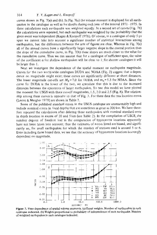
curves shown in Fig. 7(a) and (b). In Fig. 7(a) the volume moment is displayed for all earth- quakes in the catalogue as well as for shocks during each year of the interval 1971-1975. In these calculations each earthquake was weighted equally. In a second set of curves (Fig. 7b) the calculations were repeated, but each earthquake was weighted by the probability that the given event was independent (Kagan & Knopoff 1976). Of course, in a catalogue of only 5-yr span we cannot take into account a significant number of statistical interactions among earthquakes, but the differences between the sets of figures are clear. Whereas in Fig. 7(a) all of the annual curves have a significantly larger negative slope in the central portion than the slope of the cumulative curve, in Fig. 7(b) these slopes are much closer to the value for the cumulative curve, Thus we can assume that for a catalogue of sufficient span, the value of the coefficient (II for shallow earthquakes will be close to 1 ; for shorter catalogues it will be larger than 1.

Next we investigate the dependence of the spatial moment on earthquake magnitude. Curves for the two world-wide catalogues DUDA and NOAA (Fig. 3) suggest that a depen- dence on magnitude might exist; these curves are significantly different at short distances. The lower magnitude cut-offs are M s = 7.0 for DUDA and mb=5.3 for NOAA. Since the curve for DUDA is the lower of the two, we speculate that this is due to the increased distances between the epicentres of larger earthquakes. To test this model we have plotted the moment for USGS with three cut-off magnitudes, 1.5,2.0 and 2.5 (Fig. 8). The relation- ship among these curves is opposite t o that of Fig. 3. For these data the rms location errors (Lester & Meagher 1978) are shown in Table 2.

Some of the published standard errors in the USGS catalogue are unreasonably high and include nominal errors in focal depths that are sometimes as great as 300 km. We have there- fore repeated the calculations after deleting those earthquakes with nominal standard error in depth location in excess of 20 and 5 km (see Table 2). In the compilation of USGS, the number degrees of freedom lost in the computation of hypocentre locations apparently have not been taken into account; thus the estimates of errors listed are biased, and signifi- cantly so, for small earthquakes for which the number of stations used is around 5 or 6. Even including these biased data, we see that the accuracy of hypocentre locationsis strongly dependent on magnitude.

Y. Y. Kagan and L. Knopoff

! 00

1 .oo

0 -50

0.20

0.10

0 .05

0.02

0.01

0 T O T A L , N- 5586 3772.4 0 1971 E26 630.6

+ 1973 1065 763.0 x 1974 935 732.1 0 1975 1093 814.5

A 1972 1607 az0.2

0.1 1 .o 10.0 100.0 1000.0

D I S T R N C E KM

Figure 7. Time dependence of spatial volume moments. (a) Equal weights. Number of earthquakes in each catalogue indicated. (b) Weights proportional to probability of independence of each earthquake. Number of weighted earthquakes in each catalogue indicated.

Spatial distribution of earthquakes 315

c a n.

Figure

1 .oo

0.50

0.20

0.10

0.05

0 .02

0.01

0 USGS, M2.0 ~=2190 A USGS, M 2 . 5 N=687 + NOAA, ~ ~ 7 0 ~ f i f i ? 5 . j , ~ 4 9 8 2 x NOAA, n170~~lM16.0, ~=673

0.1 1 . o 10'.0 100.0 1000

DISTRNCE KH

8. Spatial volume moments for catalogues with different magnitude cut-offs.

Table 2. USGS catalogue location errors.

Magnitude

M > 1.5 M > 2.0 M > 2.5

Vertical error (ERZ) unbounded

Number of earthquakes (n) 5689 2238 709

Average vertical error (ERZ) 6.25 1.13 0.94 -

Average horizontal error (ERH) 1.47 0.82 0.6 I

I 1 __ ERZ

ERH -

ERZ < 20km

5682 2238

1.41 1.13

0.88 0.82

ERZ < 5 km

5628 2224

1.05 0.95

0.7 1 0.67

709

0.94

0.61

706

0.83

0.60

The same conclusion could be drawn from the first two statistical moments, which are rhe mean and standard deviation of the depth distribution for earthquakes with magnitudes Jf> 1.5, 2.0 and 2.5. These moments are 6.23 k 2.8 1,6.5 1 * 2.64 and 6.8 1 ? 2.47 km respec- tively. The variances decrease with increasing cut-off magnitude instead of the reverse as might have been expected if the distances between strong earthquakes had been larger th& between weaker shocks. The decrease of the standard deviation, as the magnitude cut-off increases is also probably connected with an improved accuracy of hypocentre determina- tion for stronger shocks: the total variation is some sum of the intrinsic variation of the depth distribution and statistical errors of location.

Thus we assume that the differences between the three curves USGS in Fig. 8 are caused mainly by location errors. The two curves for the NOAA catalogue (Fig. 8) show a similar behaviour: larger earthquakes appear to be more closely spaced than weaker ones. The effect here is small and possibly could also be explained by differences in the accuracy of locations.

316

The differences between the DUDA and NOAA curves (Fig. 3) seem to be attributable to the same effect. The DUDA catalogue includes earthquakes from 1905 onward; in the early years the accuracy of location was poor. If we compare the DUDA curve of Fig. 3 and the location error curve of Fig. 4, we infer that the average location errors in DUDA are of the order of 50-70 km. Some of the discrepancies may also be caused by misidentification of shallow and intermediate events in the DUDA catalogue. We conclude that there is no evidence of a variation of the spatial distribution of earthquakes with magnitude.

Y. Y. Kagan and L. Knopoff

7 Depth dependence

To study the dependence of the spatial moment on depth, the NOAA catalogue was sub- divided into five parts according to the depth range of hypocentres and the volume moment computed separately for each (Fig. 9a). The DUDA catalogue was also divided into three parts and the earliest portion of the catalogue (1905-1920) was excluded from the compu- tation because we expect the location errors to be much greater in this part of the catalogue (Fig. 9b).

The middle portions of the curves, in the distance range 50-2000 km, can be easily approximated by straight lines. The left-hand parts of the curves are influenced by location errors as discussed above. The curves indicate that the spatial moments are proportional to R" with QI changing from 1 .O for the shallow earthquakes to about 1.5 for deeper events.

The curves for catalogue NZ (Fig. 10) have a similar pattern. Although the number of hypocentres is relatively small and the ratio of the location errors to the maximum diameter of the area is larger than for the NOAA catalogue, a comparison of the curves for shallow and intermediate earthquakes provides similar results. Evidently the coefficient (Y has a higher value for intermediate than for shallow shocks. As in the case of catalogue JP (see Fig. 6b), the differences between the curves in the time intervals 1940-1966 and 1967- 1977 can be attributed to improved accuracy of earthquake location over the last decade.

10.00

5.00

2 . 0 0

I . o o

0 .SO

0.20

g 0 . 1 0 L

k (r 10.00

5 .oo

2.00

1 . o o

0 .so

0.20

0.10 10.0 100.0 1000.0 10000.0 1 00000 .o

O I S T R N C E KPI

Figure 9. Spatla\ vdume moments. (a) NOAA catalogue (1965-1911). (b) DUDA catalogue (1921- 1977).

Spatial distribution of earthquakes 317 1 .oo

0 .so

0.20

0 .10

0.05

0 . 0 2

0.01 1 .O 1 0 . 0 100.0 1000.0 10000.0

OISTRNCE K H

Figure 10. Spatial volume moments, NZ catalogue.

8 Discussion

If we combine our results from the analysis of different catalogues, we conclude that, for shallow earthquakes, the volume moment, in the distance range 0-2000 km, is proportional to R-l. This means that the set of shallow earthquake foci has the same second-order proper- ties as a uniform distribution of hypocentres on an infinite plane (as noted in Section 3 the conditional first-order volume moment defines the second-order or two-point properties of the earthquake spatial distribution). It can be argued that this result is a trivial one, because earthquake hypocentres are aligned along planar features. But even a cursory survey of epicentre maps (see, for instance, Figs 1 and 2 ) shows that, first, the distribution of epicentres along faults is not uniform and, second, there are many faults. A non-uniform distribution of hypocentres, such as a doubly-stochastic Poisson field (Cox & Lewis 1966) on one plane, or a uniform distribution of earthquakes on several faults, would not yield a second-order moment that is proportional to R-' because both of these 'simple' models have an intrinsic scale; the scale in the first model corresponds to a correlation length of inhomo- geneities along the plane; in the second scheme the scale is defined by the average distance between the faults and the mean dimensions of the faults. Of course there are infinitely many, more complex distributions of faults and/or earthquakes along the faults that have a volume moment proportional to 1/R. Because they are all stochastically equivalent to a plane, we say that they have the fractal dimension 2 (Mandelbrot 1977). A uniform plane distribution of hypocentres and a presumed distribution along well-defined earthquake faults may give the same statistical results, if those faults are distributed according to some still unknown distribution. Perhaps a study of the higher-order spatial moments of the earthquake process will provide further insight into this problem (cf. Fry & Peebles 1978).

The power-law character of the moment means that the spatial distribution of a set of earthquake foci is stochastically self-similar up to distances of the order of 2000 km and the set has no intrinsic scale. Thus it is not possible to determine the scale of a hypocentre map in the absence of location errors, without additional information. The exponent in the power-law of the moment function restricts our choice of possible models of the distribution of faults. For example a spatially homogeneous distribution of faults or cracks in an elastic medium which has a moment that is asymptotically proportional to Ro is not allowed (Kagan & Knopoff 1978).

We also remark that changes in the spatial moments with time (Fig. 7a, b) raise the possibility that it might be feasible to use these moments to identify those places where there is a deficit of shocks, i.e. a seismic gap; thus, it may be possible to use these results in seismic risk prediction.

318 Y. Y. Kagan and L. Knopoff 1 . o o

0 .so

Figure

a - c U C L

11.

0.20

0 . 1 0 1000.0 1 0 0 0 0 . 0

D I S T f i N C E K M Theoretical and experimental spatial moments on the surface of a sphere.

We discuss two additional details of the spatial distribution: the behaviour of the curves for distances greater than 2000 or 3000km and the geometry of deep earthquake faulting. From Figs 3 and 9(a), (b), the right-hand parts of the curves for shallow earthquakes indicate the moment varies approximately as Ro in this distance range. One possible explanation is that for distances greater than 2000-3000 km, the earthquake zones become more or less statistically independent. In this case, we would have a two-scale picture (Mandelbrot 1977) in which there is a dominance of linear or planar features at short range and relatively independent spatial features, such as large tectonic plates, at greater distances.

Since the large tectonic plates have a rough polyhedral pattern, we have investigated whether the worldwide distribution of shallow seismicity is statistically equivalent to any of the regular polyhedral surfaces. In Fig. 11 the NOAA curve (h < 35 km) is compared with the spatial correlation functions we would obtain had all the world’s seismicity been distri- buted uniformly along the edges of the central projection onto a sphere of the three regular polyhedra having triple junctions at their vertices. The calculations were made by numerical integration for the neighbouring edges and by Monte Carlo simulations for the larger distances. The great circle curve from Fig. 4 is also shown for comparison.

The left part of the NOAA curve is close to the curve for a tetrahedron, but the vertical position of the line (Fig. 9a) is strongly dependent on focal depths; thus the curve may be biased upwards due to ‘contamination’ by deeper shocks. The height of the curves for short range is determined by the total length of the seismic belts and by the variation of seismicity along these belts. As shown above, shallow seismicity, up to distances of 2000 km, is statistic- ally equivalent to a plane, i.e. we may consider it as uniformly distributed along the seismic belts. An obvious inconsistency with this result arises from the differences in the levels of seismicity between the oceanic rifts and the subduction zones; in view of this difference, the spatial moment is probably mainly descriptive of the distribution of the subduction zones.

With regard to the total length of the earthquake belts of the world, a rough estimate gives a value of about 120000-140000 km, which is rather consistent with the length of the edges of the dodecahedron which is 139000km. The corresponding dimension for a cube is only 94000 km. While this dimension might be appropriate for an octahedron, this latter polyhedron does not have vertices that are triple junctions. This is unfortunate since we normally count about eight large tectonic plates. Furthermore, it seems that the behavioni of the NOAA curve for larger distances, which corresponds to the breakdown of the 1 il law, may also be approximated better by the function for a dodecahedron (Fig. 11). We h m not tried the case of a random tesselation of a spherical surface for the purposes of genem ing a comparison structure (Miles 1971). In this latter case we would probably smooth ow

Spatial distribution of earthquakes 319

the kinks in the right-hand part of the diagram, which are due to the regularity of the polyhedra.

The geometry of the pattern of deeper earthquakes is a problem we are unable to solve due to the unavailability of catalogues of deeper events which are accurate and extensive. We cannot test for the presence of stochastic self-similarity in the spatial distribution of deep and intermediate events down to very small distances. But if self-similarity should be a valid description of earthquake occurrence at these depths, the fractal dimension of the set of deep earthquakes is probably close to 1, i.e. this set is stochastically equivalent to a line. For the shocks in the NOAA catalogue in the depth range 281-700 km, our estimate of a in the formula R-@ is close to 1.5. The fractal dimension is (3 -.). However, the number of earthquakes is only 429 and we are averaging over a very broad depth interval, so there are large uncertainties connected with the value of a.

An alternative explanation of the difference in the values of a between shallow and deep earthquakes is that it is due to differing time-scales for seismicity at differing depths. From Fig. 7(a) we see that an average taken over short time intervals yields larger values of a. Thus we conjecture that, for example, about 11 yr of NOAA catalogue data might be sufficient for the value of (Y for shallow earthquakes to attain its asymptotic value of 1.0, but 11 yr might not be long enough for deeper earthquakes. We do not have the catalogue data at present t o resolve these alternative models.

9 Conclusions

A statistical analysis of the spatial distributions of earthquake hypocentres in several catalogues shows:

1. Hypocentre maps have the same appearance regardless of scale. 2. After the non-uniformity of a vertical distribution of earthquakes is taken into

account, the conditional number of shallow earthquakes in a sphere of radius R centred on any of these hypocentres is proportional to R 2 in the distance range 0-2000. Thus the spatial distribution of shallow earthquakes is equivalent to a uniform distribution on an infinite plane.

3. Although the quality and quantity of deep earthquake data are much inferior t o those for shallow events, there are indications, that these earthquakes have a similar geometrical distribution with conditional moment proportional to R-3'2.

4. No evidence was found that the spatial distribution is dependent on magnitude.

Acknowledgments

This research was supported by Grants ENV76-01706 and PFR77-24742 of the ASRA programme of the National Science Foundation. The authors thank Dr W. H. K. Lee of the Lnited States Geological Survey, Dr W. D. Smith of New Zealand Seismological Observatory, Dr S . J. Duda of Seismological Institute, Uppsala, and the Japan Meteorological Agency for compiling and providing us with catalogues. The authors are grateful to Drs D. Vere-Jones, D. Perkins and J. Dewey for their comments.

Publication Number 1892, Institute of Geophysics and Planetary Physics, University of California, Los hge les .

References a, M. & Duda, S. J . , 1979. Some aspects of global seismicity, Report No. 1 - 7 9 , Seismological

Institute, Uppsala, 39 pp.

3 20 Cox, D. R. & Lewis, P. A. W., 1966. The Statistical Analysis of Series of Events, Methuen, London,

Duda, S. J., 1965. Secular seismic release in the circumPacific belt, Tectonophysics, 2,409-452. Fisher, R. A., 1928. General sampling distribution of the multiple correlation coefficient, Proc. R. SOC.

Fry, J. N. & Peebles, P. J. E., 1978. Statistical analysis of catalogs of extragalactic objects. IX. The four-

Hammersley, J. M., 1950. The distribution of distance in a hypersphere,Anri. Math. Stat., 21,447-452. Japan Meteorological Agency. Seismological bulletin of Japan Meteorological Agency, Supplementary

Kagan, Y. & Knopoff, L., 1976. Statistical search for non-random features of the seismicity of strong

Kagan, Y. & Knopoff, L., 1978. Statistical study of the occurrence of shallow earthquakes. Geophys.

Kagan, Y. Y . & Knopoff, L., 1980. Dependence of seismicity on depth, Bull. seisix SOC. Am., in press. Kendall, M. G . & Moran, P. A. P., 1963. GeometricalF’robabilities, Hafner, New York, 125 pp. Lester, F. W. & Meagher, K. L., 1978. Catalog oj earthquakes alorig Sail Andreasfault system ii7 Central

California for the year 1974, Open-file Report, US Geological Survey, 89 pp. Mandelbrot, B. B., 1977. Fractals: Form, Chance, and Dimension, W. H. Freeman, San-Francisco, 365 pp. Matheron, G., 1968. Osnovy Arkladnoi Geostastistiki, Mir, Moscow, 408 pp (in Russian). Matheron, G., 1971. The Theory of Regionalized Variables and its Applications, Cahiers du Centre d e

Miles, R. E., 1971. Random points, sets and tesselation on the surface of a sphere, Sankhya, Srr. A . 33,

Smith, W . D., 1976. Computer file of New Zealand earthquakes, N. Z. J . Geol. Geophys.. 19. 393-394.

Y. Y. Kagan and L. Knopoff

285 pp.

Lond., A , 121,654-673.

point galaxy correlation function, Adroplzys. J., 221, 19-33.

V O ~ . 1 - 1958, Vol. 2 - 1966, Vol. 3 - 1968.

earthquakes, Phys. Earth planet. Iiiteriors, 12, 291-318.

J. R. astr. Soc., 55, 67-86.

Morphologie Mathematique de Fontainebleau, No. 5, 21 1 pp.

145 - 174.