X Cd C > - Dartmouth Collegecarlp/longgaps.pdf · 2 KEVIN FORD, SERGEI KONYAGIN, JAMES MAYNARD,...

.

LONG GAPS IN SIEVED SETS

KEVIN FORD, SERGEI KONYAGIN, JAMES MAYNARD, CARL POMERANCE, AND TERENCE TAO

ABSTRACT. To each prime p, let Ip ⊂ Z/pZ denote a collection of at most C0 residue classesmodulo p, whose cardinality |Ip| is equal to 1 on the average. We show that for sufficiently large x,the sifted set {n ∈ Z : n (mod p) 6∈ Ip for all p 6 x} contains gaps of size x(log x)1/ exp(CC0) foran absolute constant C > 0; this improves over the “trivial” bound of� x. As a consequence, weshow that for any degree d polynomial f : Z→ Z mapping the integers to itself with positive leadingcoefficient, the set {n 6 X : f(n) composite} contains an interval of consecutive integers of length> (logX)(log logX)1/ exp(Cd) for some absolute constant C > 0 and sufficiently large X .

CONTENTS

1. Introduction 12. Overall strategy 63. Correlations 124. Computing correlations 15Appendix A. Proof of the covering lemma 22References 26

1. INTRODUCTION

In this paper, we will show the existence of large gaps within sets formed by sieving out from theintegers a bounded number of residue classes modulo each prime. The setup will be as follows.

Definition 1 (Sieving system). Let P = {2, 3, 5, . . . } denote the primes. A sieving system is acollection I = (Ip)p∈P of sets Ip ⊂ Z/pZ of residue classes modulo p for each prime p ∈ P .We say that the sieving system is non-degenerate and C0-bounded if the cardinalities |Ip| obey thebound

(1.1) |Ip| 6 max(C0, p− 1) (p ∈ P).

KF was supported by National Science Foundation grant DMS-1501982. JM was supported by a Clay ResearchFellowship and a Fellowship of Magdalen College, Oxford. TT was supported by a Simons Investigator grant, the Jamesand Carol Collins Chair, the Mathematical Analysis & Application Research Fund Endowment, and by NSF grant DMS-1266164. Part of this work was carried out at MSRI, Berkeley during the Spring semester of 2017, supported in part byNSF grant DMS-1440140.

2010 Mathematics Subject Classification: Primary 11N35, 11N32, 11B05.Keywords and phrases: gaps, prime values of polynomials, sieves.

1

2 KEVIN FORD, SERGEI KONYAGIN, JAMES MAYNARD, CARL POMERANCE, AND TERENCE TAO

We say that the sieving system is one-dimensional if we have the weighted prime number theorem1

(1.2)∑p6x

|Ip| =x

log x+O

(x

log x(log2 x)2

).

For any integer b, bounded set J ⊂ R and sieving system I, we define the sifted set SJ(b, I) ⊂ Zby the formula

SJ(b, I) := {n ∈ Z : n− b (mod p) 6∈ Ip ∀p ∈ J ∩ P}.Remark 1. If |Ip| = p for some p ∈ J (the degenerate case), then clearly SJ(b, I) is empty.Otherwise, SJ(b, I) is a PJ - periodic set with density σJ(I), where PJ and σJ(I) are defined as

(1.3) PJ :=∏p∈J

p, σJ(I) :=∏p∈J

(1− |Ip|

p

).

The b parameter just shifts the sifted sets SJ(bJ , I) by translation:

(1.4) SJ(b, I) = b+ SJ(0, I).The main result of this paper establishes somewhat large gaps inside non-degenerate C0-bounded

sifted sets.

Theorem 1 (Main theorem). Let I = (Ip)p∈P be a non-degenerate, C0-bounded one-dimensionalsieving system for some C0 > 1. Then, for all sufficiently large numbers x, the sifted set S[2,x](0, I)contains a gap of length at least x(log x)1/ exp(CC0) for some absolute constant C > 0.

Remark 2. Note that by (1.4), to prove Theorem 1 it is sufficent to show there is some b ∈ Z/P[2,x]Zwith

S[2,x](b, I) ∩ [1, x(log x)1/ exp(CC0)] = ∅.The conclusion of Theorem 1 should be compared with the “trivial” bound

(1.5) S[2,x](b, I) ∩ [1, c′x] = ∅for some constant c′ > 0 and large x. To deduce this, we first use (1.1), (1.2), and partial summation,to obtain a Mertens-type product estimate

(1.6) σ[2,z](I) =∏p6z

(1− |Ip|

p

)=

C1

log z

(1 +O

(1

log2 z

)),

where C1 is a certain positive constant (in general, C1 depends on the behavior of |Ip| for small p,and can have great variation even over systems with a constant C0). If x is large, then it followsthat there is some b modulo P[2,x/2] for which A := S[2,x/2](b, I) ∩ [1, x/(8C0C1)] satisfies |A| 6

x4C0 log x

. On the other hand, by (1.2), ∑x/2<q6x

|Iq| ∼x/2

log x

and hence by (1.1),

(1.7) #{x/2 < q 6 x : |Iq| > 1} > x

4C0 log x.

1The notation log2 x means log log x, log3 x means log log log x, etc. The symbol p always denotes a prime.

LONG GAPS IN SIEVED SETS 3

Hence, we may pair up each element a ∈ A with a unique prime q = qa ∈ (x/2, x] for which|Iq| > 1. For each such pair a, qa let va ∈ Iqa and suppose that b ≡ a− va (mod q). It follows thatS[2,x](b, I) ∩ [1, x/(8C0C1)] = ∅, proving (1.5).

Example 1. The “Eratosthenes” sieving system I = ({0 (mod p)})p∈P is non-degenerate, 1-bounded, and 1-dimensional. The Eratosthenes sieve asserts that

(1.8) P ∩ (√x, x] = S[2,

√x](0, I) ∩ (

√x, x].

The problem of finding large gaps between consecutive primes has a long history, and it is currentlyknown that gaps of size

(1.9) � log xlog2 x log4 x

log3 x

exist below x if x is large enough [7]; this improves over the “trivial” bound of� log x from theprime number theorem or the more elementary Chebyshev estimates. The existing methods forfinding large gaps between primes, however, seem not to be adaptable to find large gaps in moregeneral sieving systems. We will discuss the reasons for this in detail below. Our proof of Theorem1 follows a very different route, relying on a new probabilistic method.

Example 2. Given a polynomial f : Z→ Z of degree d > 1, the system

Ip := {n ∈ Z/pZ : f(n) ≡ 0 (mod p)}

is d-bounded, and is non-degenerate if and only if there does not exist a prime p that divides all thevalues f(n), n ∈ Z. For irreducible f , the 1-dimensionality (1.2) follows quickly from Landau’sPrime Ideal Theorem [13] (see also [3, pp. 35–36]). As a variant of (1.8), we observe that

(1.10) {n ∈ A : f(n) ∈ P} ⊂ S[2,x](0, I)

for any x > 1 and any set A such that f(n) > x for all n ∈ A. Now set x := 12 logX . By Theorem

1, the set S[2,x](0, I) contains a gap of length� logX(log2X)1/ exp(Cd). The period of this set isP[2,x], which by the prime number theorem is X1/2+o(1). Thus, this set contains such a long gapinside the interval [X/2, X]. Assuming that f has a positive leading coefficient and that X is large,on this interval, f(n) > x, and hence f(n) is composite for every n ∈ [X/2, X]\S[2,x](0, I). Wethus obtain the following.

Theorem 2. Let f : Z → Z be a polynomial of degree d > 1 with positive leading term. Thenfor sufficiently large X , there is a string of consecutive natural numbers n ∈ [1, X] of length> logX(log2X)1/ exp(Cd) for which f(n) is composite, for some absolute constant C > 0.

We note that when f has degree two or greater, it is still an open conjecture (of Bunyakovsky [1])that there are infinitely many n for which f(n) is prime; we do not address this conjecture at all inthis paper. Also, Theorem 2 follows trivially in the “degenerate” cases, when either f is reducible,or there is some prime p with |Ip| = p.

Remark 3. While the polynomial f must be in Q[x], it need not have integer coefficients, e.g.f(n) = n7−n+7

7 satisfies the hypotheses of Theorem 2.


Example 3. A simple example to keep in mind (and in fact the original example we studied) isf(n) = n2 + 1. In this case, I2 = {1}, Ip is empty for p ≡ 3 (mod 4), and Ip = {ιp,−ιp} forp ≡ 1 (mod 4), where ιp ∈ Z/pZ is one of the square roots of −1. Here one can use the primenumber theorem in arithmetic progressions rather than the Prime Ideal theorem to establish one-dimensionality. For this example (and for any quadratic polynomial), our methods produce (takingM = 4 + 10−15 in (2.1)) consecutive composite strings of length � (logX)(log2X)K2 , whereK−12 ≈ 1.144× 1020. It is certain that further numerical improvements are possible.

S: Another applicationof Theorem 1 forpolynomials is included

Theorem 1 has another application, to a problem on the coprimality of consecutive values ofpolynomials.

Corollary 1. Let f : Z → Z be a non-constant polynomial. Then there exists an integer Gf > 2such that for any integer k > Gf there are infinitely many integers n > 0 with the property thatnone of f(n+ 1), . . . , f(n+ k) is coprime to all the others.

Proof. Let d = deg f . Then d!f(x) ∈ Z[x]. Let f0(x) ∈ Z[x] be a primitive irreducible factorof d!f(x). If p > d is a prime and p | f0(m) for some integer m, then p | f(m). So it willsuffice to consider the case that f is irreducible and show in this case that for all large k there areinfinitely many n > 0 such that for each i ∈ {1, . . . , k} there is some j ∈ {1, . . . , k} with j 6= iand gcd(f(n+ i), f(n+ j)) divisible by some prime > d.

Again, we consider the system I defined by

Ip := {n ∈ Z/pZ : f(n) ≡ 0 (mod p)},but for p 6 d, we take Ip = ∅. By Theorem 1, for all sufficiently large numbers x the set S[2,x](0, I)contains a gap of length > k = b2xc. Thus, there are infinitely many n such that each f(n +1), . . . , f(n+ k) has a prime factor p with d < p 6 x. For each i ∈ {1, . . . , k}, take a prime factorp of f(n+ i) with d < p 6 x. Since k = b2xc, p 6 x and Ip 6= ∅, it must be that p divides at leasttwo terms of the sequence f(n+ 1), . . . , f(n+ k), thus proving the assertion. �

For linear polynomials the result of the corollary is well-known. For quadratic and cubic polyno-mials in Z[x] it was recently proven by Sanna and Szikszai [15].

1.1. Discussion of methods. In the case of the Eratosthenes sieving system I = (0 (mod p))p∈P ,for any set J and shift b, the largest gap in the infinite periodic set SJ(b, I) is equal to j(PJ), wherej(n) is Jacobsthal’s function of n, defined as the largest gap between the integers coprime to n. Thebest bounds known for j(P[2,x]) for primorials P[2,x] are

(1.11)x log x log3 x

log2 x� j(P[2,x])� x2

for sufficiently large x; see [7] for the lower bound and [11] for the upper bound. Combining thelower bound in (1.11) with the sieve of Erathosthenes (1.8) gives the lower bound (1.9) for largegaps between primes obtained in [7]. The implication only works in one direction; the upper boundin (1.11) is not known to imply any upper bound on gaps between primes. We refer the reader to [7]for further discussion and for a history of the problem.

For the Eratosthenes sieving system I = (0 (mod p))p∈P , it is clear that S[2,x](0, I) avoids theinterval [2, x], which already gives the “trivial” lower bound j(P[2,x]) � x. Most of the improve-ments to this bound in previous literature (including those in [7]) rely on the following variant of this


observation: if x > z > 2, then the sifted set S(z,x](0, I), when restricted to the interval [1, y) withy slightly larger than x, only consists of numbers of the form a or ap, where p is a prime in (x, y],and a is a z-smooth (or z-friable number), which means that all the prime factors of a do not exceedz. Using the known bounds on the frequency of smooth numbers (see e.g. [2]), the set of numbersof the first type a can be made to be negligible by choosing z appropriately, leaving one with a setwhich is essentially a collection of primes p (the additional factor of a in ap can be eliminated byworking with numbers close to x and doing some additional sieving at very small primes). Mostof the remaining effort in establishing lower bounds for j(P[2,x]) then goes into covering this col-lection of primes with congruence classes as efficiently as possible. The most recent works in thisdirection [14, 6, 7] rely on recent results concerning tuples of linear forms that attain many primevalues simultaneously, with the bounds in [7] also relying on a combinatorial hypergraph coveringlemma of Pippenger-Spencer type. Again, we refer the reader to [7] for further discussion.

Unfortunately, when considering the more general sieving systems in Definition 1, in which thecardinalities |Ip| are allowed to vanish for many primes p, bounds for smooth numbers cannot beused to bound S(z,x](0), and without this first crucial step the existing methods only yield the triviallower bound of � x for the gap size. We overcome the barrier by using a very different method;rather than choosing a specific b for some interval J , we make a random choice of b; this is donevia the Chinese Remainder Theorem by choosing b mod p for primes p ∈ J at random, but witha complex dependency structure. This will be described in full in the next section. As in [7], weutilize a hypergraph covering lemma to obtain the best bounds, though it is possible to obtain weakerimprovements to the trivial bound (gaining a small power of log2 x rather than log x in Theorem 1)without using such a lemma.

Remark 4. Unfortunately our methods only seem to give good results in the one-dimensional case.Consider for instance the set {n ∈ P : n+ 2 ∈ P} of (the lower) twin primes. This corresponds toa two-dimensional system in which Ip = {0 (mod p), 2 (mod p)} for all primes p. The “trivial”bound coming from these methods would give a bound of � logX log2X for the largest gapbetween lower twin primes up to X (or between the largest such twin prime and X), and one couldpossibly hope to improve this bound by a small power of log2X; however, a sieve upper bound(e.g., [9, Cor. 2.4.1]) combined with the pigeonhole principle already gives a bound of� log2Xin this case.

1.2. Notation. We use X � Y, Y � X , or X = O(Y ) to denote the estimate |X| 6 CY forsome constant C > 0, and write X � Y for X � Y � X . Throughout the remainder of the paper,we adopt the convention that all implied constants in O- and related order estimates may depend onC0, C1 and the implied constants in the O-bounds in the estimates (1.2) and (1.6). Constant impliesby O- and related symbols will not depend on any other quantity. We also assume that the quantityx is sufficiently large in terms of all of these parameters.

The notation X = o(Y ) as x→∞ means limx→∞X/Y = 0 (holding other parameters fixed).If S is a statement, we use 1S to denote its indicator, thus 1S = 1 when S is true and 1S = 0

when S is false.We will rely on probabilistic methods in this paper. Boldface symbols such as n, S, λ etc. denote

random variables (which may be real numbers, random sets, random functions, etc.). Most of theserandom variables will be discrete (in fact they will only take on finitely many values), so that we mayignore any technical issues of measurability; however it will be convenient to use some continuous


random variables in the appendix. We use P(E) to denote the probability of a random event E, andEX to denote the expectation of the random (real-valued) variable X.

For a natural number d, we use ω(d) to denote the number of primes p with p | d.Unless specified, all sums are over the natural numbers. An exception is made for sums over the

variables p or q (as well as variants such as p1, p2, etc..), which will always denote primes.Given two subsets A,B of an additive group G, we define the sumset and difference set

A+B := {a+ b : a ∈ A, b ∈ B},A−B := {a− b : a ∈ A, b ∈ B}.

Similarly we define the translatesA+ h = h+A := {a+ h : a ∈ A},

A− h := {a− h : a ∈ A}for h ∈ G, and for any integer n, we define the dilate

n ·A := {na : a ∈ A}.

2. OVERALL STRATEGY

In this section we describe the high-level strategy of proof, and perform two initial reductions onthe problem, ultimately leaving one with the task of proving Theorem 3 below.

Let I be a non-degenerate, C0-bounded one-dimensional sieving system. Let ε > 0 be anarbitrarily small, fixed real number, and let M > 1 be a fixed, positive real number which willbe optimized later. Suppose x is large (think of x→∞), and define the quantities y and δ1 as

(2.1) y := x(log x)δ1 , δ1 :=1− ε

M exp(5.6MC0).

Our goal is to show that S[2,x](b, I) ∩ [1, y] = ∅ for some b. We make two trivial observations:• A linear shift of any single set Ip (that is, replacing Ip by c+ Ip for some integer c) does not

affect the structure of SJ(b, I) (up to changing the b parameter). Thus, the same is true forlinear shifts (depending on p) for any finite set of primes p. In particular, we may shift thesets Ip so that all nonempty sets Ip contain the zero element, without changing the structureof SJ(b, I).• The set SJ(b, I) depends only on b modulo PJ . By the Chinese Remainder Theorem,b mod PJ is uniquely determined by the set of residue classes b mod p for primes p ∈ J .

Therefore, we may assume without loss of generality that 0 ∈ Ip whenever Ip is nonempty, and wewill select b by choosing residue classes b modulo primes p 6 x. We introduce the parameter

(2.2) z :=y

(log x)(1−ε)/M,

so that for x large enough we have

1 6 z 6 x/2 6 x 6 y.

We will select the parameter b modulo the primes p 6 x in three stages:(1) (Uniform random stage) First, we choose b modulo P[2,z] uniformly at random; equiva-

lently, for each prime p 6 z, we choose b mod p randomly with uniform probability, inde-pendently for each p;


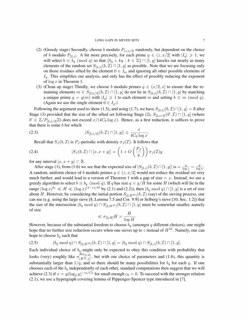
(2) (Greedy stage) Secondly, choose b modulo P(z,x/2] randomly, but dependent on the choiceof b modulo P[2,z]. A bit more precisely, for each prime q ∈ (z, x/2] with |Iq| > 1, wewill select b ≡ bq (mod q) so that {bq + kq : k ∈ Z} ∩ [1, y] knocks out nearly as manyelements of the random set S[2,z](b, I) ∩ [1, y] as possible. Note that we are focusing onlyon those residues sifted by the element 0 ∈ Iq, and ignoring all other possible elements ofIq. This simplifies our analysis, and only has the effect of possibly reducing the exponentof log x in Theorem 1.

(3) (Clean up stage) Thirdly, we choose b modulo primes q ∈ (x/2, x] to ensure that the re-maining elements m ∈ S[2,x/2](b, I) ∩ [1, y] do not lie in S[2,x](b, I) ∩ [1, y] by matchinga unique prime q = q(m) with |Iq| > 1 to each element m and setting b ≡ m (mod q).(Again we use the single element 0 ∈ Iq.)

Following the argument used to show (1.5), and using (1.7), we have S[2,x](b, I)∩ [1, y] = ∅ afterStage (3) provided that the size of the sifted set following Stage (2), S[2,x/2](b′, I) ∩ [1, y] (whereb′ ∈ Z/P[2,x/2]Z) does not exceed x/(4C0 log x). Hence, as a first reduction, it suffices to provethat there is some b for which

(2.3) |S[2,x/2](b, I) ∩ [1, y]| 6 x

4C0 log x.

Recall that SJ(b, I) is PJ -periodic with density σJ(I). It follows that

(2.4) |SJ(b, I) ∩ [x, x+ y]| =(1 +O

(PJy

))σJ(I)y

for any interval [x, x+ y] ⊂ R.After stage (1), from (1.6) we see that the expected size of |S[2,z](b, I)∩ [1, y]| is� y

log z ∼y

log x .A random, uniform choice of b modulo primes q ∈ (z, x/2] would not reduce the residual set verymuch further, and would lead to a version of Theorem 1 with a gap of size � x. Instead, we use agreedy algorithm to select b ≡ bq (mod q). If q has size q � y/H for someH (which will lie in therange (log x)δ1 � H � (log x)(1−ε)/M by (2.1) and (2.2)), then (bq mod q) ∩ [1, y] is a set of sizeabout H . However, by considering the initial portion S[2,HM ](b, I) (say) of the sieving process, onecan see (e.g. using the large sieve [8, Lemma 7.5 and Cor. 9.9] or Selberg’s sieve [10, Sec. 1.2]) thatthe size of the intersection (bq mod q) ∩ S[2,HM ](b, I) ∩ [1, y] must be somewhat smaller, namelyof size

� σ[2,H]H �H

logH.

However, because of the substantial freedom to choose bq (amongst q different choices), one mighthope that no further size reduction occurs when one sieves up to z instead of HM . Namely, one canhope to choose bq such that

(2.5) (bq mod q) ∩ S[2,HM ](b, I) ∩ [1, y] = (bq mod q) ∩ S[2,z](b, I) ∩ [1, y].

Each individual choice of bq might only be expected to obey this condition with probability that

looks (very) roughly like σHσ[2,H]

(HM ,z], but with our choice of parameters and (1.6), this quantity is

substantially larger than 1/q, and so there should be many possibilities for bq for each q. If onechooses each of the bq independently of each other, standard computations then suggest that we willachieve (2.3) if x = y(log2 y)

−c0/C0 for small enough c0 > 0. To succeed with the stronger relation(2.1), we use a hypergraph covering lemma of Pippenger-Spencer type introduced in [7].


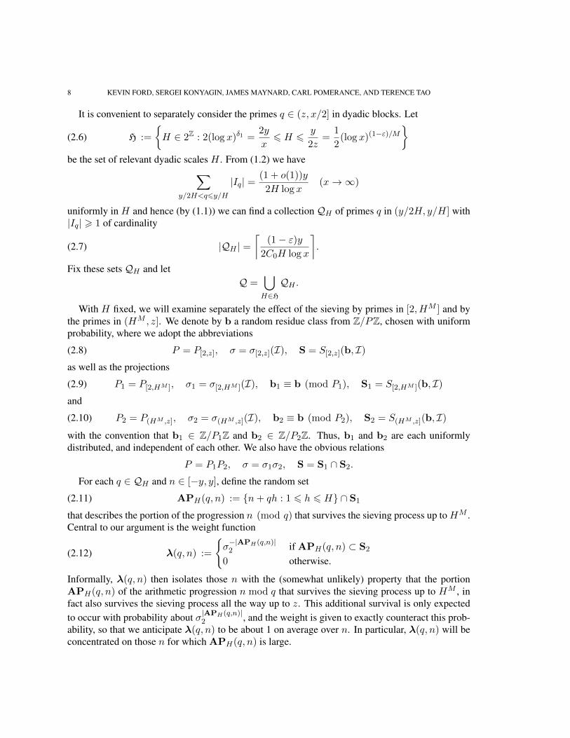
It is convenient to separately consider the primes q ∈ (z, x/2] in dyadic blocks. Let

(2.6) H :=

{H ∈ 2Z : 2(log x)δ1 =

2y

x6 H 6

y

2z=

1

2(log x)(1−ε)/M

}be the set of relevant dyadic scales H . From (1.2) we have∑

y/2H<q6y/H

|Iq| =(1 + o(1))y

2H log x(x→∞)

uniformly in H and hence (by (1.1)) we can find a collection QH of primes q in (y/2H, y/H] with|Iq| > 1 of cardinality

(2.7) |QH | =⌈

(1− ε)y2C0H log x

⌉.

Fix these sets QH and letQ =

⋃H∈HQH .

With H fixed, we will examine separately the effect of the sieving by primes in [2, HM ] and bythe primes in (HM , z]. We denote by b a random residue class from Z/PZ, chosen with uniformprobability, where we adopt the abbreviations

(2.8) P = P[2,z], σ = σ[2,z](I), S = S[2,z](b, I)as well as the projections

(2.9) P1 = P[2,HM ], σ1 = σ[2,HM ](I), b1 ≡ b (mod P1), S1 = S[2,HM ](b, I)and

(2.10) P2 = P(HM ,z], σ2 = σ(HM ,z](I), b2 ≡ b (mod P2), S2 = S(HM ,z](b, I)

with the convention that b1 ∈ Z/P1Z and b2 ∈ Z/P2Z. Thus, b1 and b2 are each uniformlydistributed, and independent of each other. We also have the obvious relations

P = P1P2, σ = σ1σ2, S = S1 ∩ S2.

For each q ∈ QH and n ∈ [−y, y], define the random set

(2.11) APH(q, n) := {n+ qh : 1 6 h 6 H} ∩ S1

that describes the portion of the progression n (mod q) that survives the sieving process up toHM .Central to our argument is the weight function

(2.12) λ(q, n) :=

{σ−|APH(q,n)|2 if APH(q, n) ⊂ S2

0 otherwise.

Informally, λ(q, n) then isolates those n with the (somewhat unlikely) property that the portionAPH(q, n) of the arithmetic progression n mod q that survives the sieving process up to HM , infact also survives the sieving process all the way up to z. This additional survival is only expectedto occur with probability about σ|APH(q,n)|

2 , and the weight is given to exactly counteract this prob-ability, so that we anticipate λ(q, n) to be about 1 on average over n. In particular, λ(q, n) will beconcentrated on those n for which APH(q, n) is large.


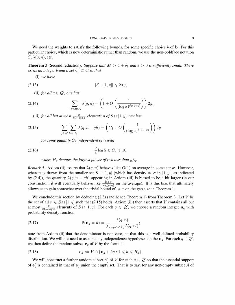
We need the weights to satisfy the following bounds, for some specific choice b of b. For thisparticular choice, which is now deterministic rather than random, we use the non-boldface notationS, λ(q, n), etc.

Theorem 3 (Second reduction). Suppose that M > 4 + δ1 and ε > 0 is sufficiently small. Thereexists an integer b and a set Q′ ⊂ Q so that

(i) we have

(2.13) |S ∩ [1, y]| 6 2σy,

(ii) for all q ∈ Q′, one has

(2.14)∑

−y<n6yλ(q, n) =

(1 +O

(1

(log x)δ1(1+ε)

))2y,

(iii) for all but at most x8C0 log x

elements n of S ∩ [1, y], one has

(2.15)∑q∈Q′

∑h6Hq

λ(q, n− qh) =(C2 +O

(1

(log x)δ1(1+ε)

))2y

for some quantity C2 independent of n with

(2.16)5

4log 5 6 C2 6 10,

where Hq denotes the largest power of two less than y/q.

Remark 5. Axiom (ii) asserts that λ(q, n) behaves like O(1) on average in some sense. However,when n is drawn from the smaller set S ∩ [1, y] (which has density ≈ σ in [1, y], as indicatedby (2.4)), the quantity λ(q, n − qh) appearing in Axiom (iii) is biased to be a bit larger (in ourconstruction, it will eventually behave like log y

log(y/q) on the average). It is this bias that ultimatelyallows us to gain somewhat over the trivial bound of� x on the gap size in Theorem 1.

We conclude this section by deducing (2.3) (and hence Theorem 1) from Theorem 3. Let V bethe set of all n ∈ S ∩ [1, y] such that (2.15) holds; Axiom (iii) then asserts that V contains all butat most x

8C0 log xelements of S ∩ [1, y]. For each q ∈ Q′, we choose a random integer nq with

probability density function

(2.17) P(nq = n) =λ(q, n)∑

−y<n′6y λ(q, n′);

note from Axiom (ii) that the denominator is non-zero, so that this is a well-defined probabilitydistribution. We will not need to assume any independence hypotheses on the nq. For each q ∈ Q′,we then define the random subset eq of V by the formula

(2.18) eq := V ∩ {nq + hq : 1 6 h 6 Hq}.

We will construct a further random subset e′q of V for each q ∈ Q′ so that the essential supportof e′q is contained in that of eq union the empty set. That is to say, for any non-empty subset A of


V , the probability P(e′q = A) is only non-zero when P(eq = A) is non-zero. Furthermore, theserandom subsets will satisfy

(2.19) E∣∣∣∣V \ ⋃

q∈Q′e′q

∣∣∣∣ 6 x

8C0 log x.

Then by Markov’s inequality, one can find, for each q, a set eq in the essential support of e′q (andhence either empty or in the essential support of eq) such that

|V \⋃q∈Q

eq| 6x

8C0 log x.

By construction, for each q ∈ Q′ there is a number nq such that

eq ⊂ {n ∈ V : n ≡ nq (mod q)}.

Taking b ≡ nq (mod q) for all q ∈ Q′, we find that∣∣S[2,x/2](b, I) ∩ [1, y]∣∣ 6 x

8C0 log x+

x

8C0 log x=

x

4C0 log x,

as required for (2.3).It remains to locate random subsets e′q obeying (2.19). A naive first attempt would be to just take

each e′q to be a copy of eq in such a fashion that the e′q are independent in q. However, if one doesthis, then the quantity |V \

⋃q∈Q′ eq| will only be smaller than |V | by a factor of about exp(−C1),

largely thanks to (2.15). This is not sufficient for our application (although a modification of thisapproach will give Theorem 1 with the quantity x(log x)1/ exp(CC0) replaced by x(log2 x)

c/C0 forsome absolute constant c > 0). Instead, we use the following hypergraph covering lemma, which isa minor variant of [7, Corollary 4]:

Lemma 2.1 (Hypergraph covering lemma). Let y be a large number, and let V,A be finite sets with|A| 6 y and |V | 6 y. For each q ∈ A, let eq be a random subset of V satisfying the size bound

(2.20) |eq| 6 r := (log y)1/2.

Also assume the following:• (Sparsity) For all q ∈ A and v ∈ V , one has

(2.21) P(v ∈ eq) 6 y−1/2−1/100.

• (Uniform covering) For all v ∈ V , one has

(2.22)

∣∣∣∣∣∑q∈A

P(v ∈ eq)− C2

∣∣∣∣∣ 6 η

500

for some quantities C2 and η, independent of v, satisfying

(2.23)5

4log 5 6 C2 6 10

and

(2.24) (log y)− log 5

4 log 10 6 η < 1.


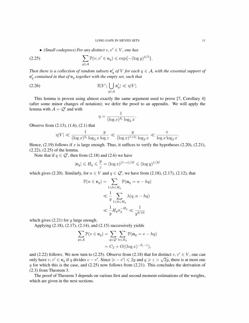
• (Small codegrees) For any distinct v, v′ ∈ V , one has

(2.25)∑q∈A

P(v, v′ ∈ eq) 6 exp{−(log y)4/5}.

Then there is a collection of random subsets e′q of V for each q ∈ A, with the essential support ofe′q contained in that of eq together with the empty set, such that

(2.26) E|V \⋃q∈A

e′q| � η|V |.

This lemma is proven using almost exactly the same argument used to prove [7, Corollary 4](after some minor changes of notation); we defer the proof to an appendix. We will apply thelemma with A = Q′ and with

η =1

(log x)δ1 log2 x.

Observe from (2.13), (1.6), (2.1) that

η|V | � 1

(log x)δ1 log2 x

y

log z� y

(log x)1+δ1 log2 x� x

log x log2 x.

Hence, (2.19) follows if x is large enough. Thus, it suffices to verify the hypotheses (2.20), (2.21),(2.22), (2.25) of the lemma.

Note that if q ∈ Q′, then from (2.18) and (2.6) we have

|eq| 6 Hq 6y

z= (log x)(1−ε)/M 6 (log y)1/M

which gives (2.20). Similarly, for n ∈ V and q ∈ Q′, we have from (2.18), (2.17), (2.12), that

P(n ∈ eq) =∑

16h6Hq

P(nq = n− hq)

� 1

y

∑16h6Hq

λ(q, n− hq)

� 1

yHqσ

−Hq2 � 1

y9/10

which gives (2.21) for y large enough.Applying (2.18), (2.17), (2.14), and (2.15) successively yields∑

q∈AP(v ∈ eq) =

∑q∈Q′

∑h6Hq

P(nq = v − hq)

= C2 +O((log x)−δ1−ε),

and (2.22) follows. We now turn to (2.25). Observe from (2.18) that for distinct v, v′ ∈ V , one canonly have v, v′ ∈ eq if q divides v − v′. Since |v − v′| 6 2y and q > z >

√2y, there is at most one

q for which this is the case, and (2.25) now follows from (2.21). This concludes the derivation of(2.3) from Theorem 3.

The proof of Theorem 3 depends on various first and second moment estimations of the weights,which are given in the next sections.


3. CORRELATIONS

We deduce Theorem 3 from the following moment calculations.

Theorem 4 (Third reduction). Assume that M > 2. We have the following:(i) One has

(3.1) E|S ∩ [1, y]|j =(1 +O

(1

(log x)1−ε

))(σy)j (j = 0, 1, 2).

(ii) For every H ∈ H,

E∑q∈QH

∑−y<n6y

λ(q, n)

j

=

(1 +O

(1

HM−2

))(2y)j |QH | (j = 0, 1, 2).

(iii) For every H ∈ H,

(3.2) E∑

n∈S∩[1,y]

( ∑q∈QH

∑h6H

λ(q, n− qh)

)j=

(1 +O

(1

HM−2

))(|QH |Hσ2

)jσy

for j = 0, 1, 2.

Note that for every n ∈ [1, y] and h 6 H we have n − qh ∈ [−y, y], so the quantity in (3.2) iswell-defined. As with the previous theorem, the quantity λ(q, n) behaves like 1 on the average whenn is drawn from [−y, y] ∩ Z, but for n drawn from S ∩ [1, y] (in particular, n ∈ S2), the quantityλ(q, n−qh) is now biased to have an average value of approximately σ−12 because n−qh+qh = nis automatically in S2; recall the definition (2.12) of λ(q, n− qh).

Deduction of Theorem 3 from Theorem 4. We draw b uniformly at random from Z/PZ. It willsuffice to generate a random set Q′ and a random function λ such that the conclusions of Theorem3 (with b replaced by b) hold with positive probability.

From Theorem 4(i) we have

E∣∣|S ∩ [1, y]| − σy

∣∣2 � (σy)2

(log x)1−ε.

Hence by Chebyshev’s inequality, we see that

(3.3) P (|S ∩ [1, y]| 6 2σy) = 1−O((log x)ε−1).

Let H ∈ H. From Theorem 4(ii) we have

(3.4) E∑q∈QH

( ∑−y<n6y

λ(q, n)− 2y

)2

� y2|QH |HM−2 .

Now let Q′H be the subset of q ∈ QH with the property that

(3.5)∣∣∣ ∑−y<n6y

λ(q, n)− 2y∣∣∣ 6 y

H1+ε.

It follows from (3.4) and (3.5) that

(3.6) E|QH\Q′H | �|QH |

HM−4−2ε .


By Markov’s inequality, it follows that with probability 1−O(H−ε), one has

(3.7) |QH\Q′H | �|QH |

HM−4−3ε .

Assume now that M > 4 + 3ε, that is, the exponent in the denominator in (3.7) is positive. Since∑H∈HH

−ε � (y/x)−ε � (log x)−δ1ε, with probability 1 − O((log x)−δ1ε) the relation (3.7)holds for every H ∈ H simultaneously. We now set

Q′ :=⋃H∈H

Q′H .

Then, on the probability 1 − o(1) event that (3.7) holds for every H and that (3.3) holds, items (i)(2.13) and (ii) (2.14) of Theorem 3 follow upon recalling (3.5) and the lower bound H � (log x)δ1 .

We work on part (iii) of Theorem 3 using Theorem 4(iii) in a similar fashion to previous argu-ments. We have

E∑

n∈S∩[1,y]

∣∣∣∣∣∣∑q∈QH

∑h6H

λ(q, n− qh)− |QH |Hσ2

∣∣∣∣∣∣2

� 1

HM−2

(|QH |Hσ2

)2

σy.

If we let EH denote the set of n ∈ S ∩ [1, y] such that

(3.8)

∣∣∣∣∣∣∑q∈QH

∑h6H

λ(q, n− qh)− |QH |Hσ2

∣∣∣∣∣∣ > |QH |Hσ2H(M−2)/2−ε ,

thenE|EH | �

σy

Hε.

By Markov’s inequality, we conclude that |EH | 6 σy/Hε/2 with probability 1−O(H−ε/2).We next estimate the contribution from “bad” primes q ∈ QH\Q′H . For any h 6 H , by Cauchy-

Schwarz we have

E∑

n∈S∩[1,y]

∑q∈QH\Q′H

λ(q, n− hq) 6(E|QH\Q′H |

)1/2E∑

q∈QH\Q′H

∣∣∑n

λ(q, n− hq)∣∣21/2

and by the triangle inequality, (3.4) and (3.6),

E∑

q∈QH\Q′H

∣∣∑n

λ(q, n− hq)∣∣2 6 2E

∑q∈QH\Q′H

(∣∣∑n

λ(q, n− hq)− 2y∣∣2 + 4y2

)

� y2|QH |HM−4−2ε .

Therefore, by (3.6) and summing over h 6 H ,

E∑

n∈S∩[1,y]

∑q∈QH\Q′H

∑h6H

λ(q, n− hq)� y|QH |HM−5−2ε .


Let E ′H denote the set of n ∈ S ∩ [1, y] so that

(3.9)∑

q∈QH\Q′H

∑h6H

λ(q, n− hq) > |QH |HH(1+ε)δ1σ2

.

Then

E|E ′H | �yHδ1(1+ε)σ2HM−4−2ε � σy

logH

HM−4−δ1−3ε .

By Markov’s inequality, |E ′H | 6 σy/Hε with probability 1−O(1/HM−4−δ1−5ε).Now suppose that

M > 4 + δ1,

ε is small enough so that M − 4 − δ1 − 5ε > ε, and that we are in the event that (3.3) holds, andthat for every H , we have (3.7), |EH | 6 σy/Hε/2 and |E ′H | 6 σy/H1+ε. This simultaneous eventhappens with positive probability on account of

∑H∈HH

−η � (log x)−δ1η for any η > 0. Asmentioned before, items (i) and (ii) of Theorem 3 hold. Now let

N = S ∩ [1, y]\⋃H∈H

(EH ∪ E ′H).

The number of exceptional elements satisfies

∣∣∣∣∣ ⋃H∈H

(EH ∪ E ′H)

∣∣∣∣∣� σy

(log x)δ1(1+ε),

which is smaller than x8C0 log x

for large x. It remains to verify (2.15) for n ∈ N . Since n 6∈ EH andn 6∈ E ′H for every H , the inequalities opposite to those in (3.8) and (3.9) hold, and we obtain

∑q∈Q′

∑h6Hq

λ(q, n− qh) =∑H∈H

∑q∈Q′H

∑h6H

λ(q, n− qh)

=

(1 +O

(1

(log x)(1+ε)δ1

))C2 × 2y

where

C2 :=1

2y

∑H∈H

|QH |Hσ2

.


From (2.7), we see that C2 does not depend on n (C2 depends only of x). Using (1.6), (2.7), (2.2),(2.1), we thus have, as x→∞,

C2 =1 + o(1)

2y

∑H∈H

log z

log(HM )

(1− ε)y2C0H log x

H

=1− ε+ o(1)

4MC0

∑H∈H

1

logH

=1− ε+ o(1)

4MC0

∑2(log x)δ162j6 1

2(log x)(1−ε)/M

1

j log 2

= (1− ε+ o(1))log(

1−εMδ1

)4MC0 log 2

= (1− ε+ o(1))

(1.4

log 2+

log(1− ε)4MC0 log 2

)>

5

4log 5,

giving (2.16) for small enough ε. �

It remains to establish Theorem 4. This is the objective of the next section of the paper.

4. COMPUTING CORRELATIONS

On account of (2.2) and (2.6), we have HM 6 (log x)1−ε and consequently

(4.1) P1 6 exp[O((log x)1−ε)

].

Hence, by (2.4), S1 has good behavior in intervals of length larger than P1, regardless of the choiceof b1.

In our verification of the claims in Theorem 4, we will frequently need to compute k-point cor-relations of the form

P (n1, . . . , nk ∈ S2)

for various integers n1, . . . , nk (not necessarily distinct). Heuristically, since S2 has density σ2,we expect these correlations to be approximately equal to σk2 for typical choices of n1, . . . , nk.Unfortunately, there is some fluctuation from this prediction, most obviously when two or moreof the n1, . . . , nk are equal, but also if the reductions ni (mod p), nj (mod p) for some primep ∈ (HM , z] have the same difference as two elements of Ip. Fortunately we can control thesefluctuations to be small on average. To formalize this statement we need some notation. Let DH ⊂N denote the collection of squarefree numbers d, all of whose prime factors lie in (HM , z]. This setincludes 1, but we will frequently remove 1 and work instead with DH\{1}. For each d ∈ DH , letId ⊂ Z/dZ denote the collection of residue classes a mod d such that a mod p ∈ Ip for all p | d.In particular we may form the difference set Id − Id ⊂ Z/dZ of Id. For any integer m and anyparameter A > 0, we define the error function

(4.2) EA(m) :=∑

d∈DH\{1}

Aω(d)

d1m (mod d)∈Id−Id ,


where we recall that ω(d) is the number of prime factors of ω. The quantity EA(m) looks compli-cated, but in practice it will be quite small as soon as we are able to perform any sort of averagingin m. We also observe that EA is an even function: EA(−m) = EA(m).

We then have

Lemma 4.1. Let 1 6 k 6 10H , and suppose that n1, . . . , nk are integers (possibly with repetition),and that M > 2. Then we have

P(n1, . . . , nk ∈ S2) =

1 +O

(k2

HM

)+O

1

k2

∑16i<j6k

EC0k2(ni − nj)

σk2 .

Proof. For each prime p ∈ (HM , z], let b2,p ∈ Z/pZ be the reduction of b2 modulo p, thus eachb2,p is uniformly distributed in Z/pZ and the b2,p are independent in p. Let Np denote the set ofresidue classes {n1 (mod p), . . . , nk (mod p)}. By the Chinese remainder theorem, we thus have

P(n1, . . . , nk ∈ S2) =∏

p∈(HM ,z]

P(n1 (mod p), . . . , nk (mod p) 6∈ b2,p + Ip)

=∏

p∈(HM ,z]

(1− P(b2,p ∈ Np − Ip))

=∏

p∈(HM ,z]

(1− |Np − Ip|

p

)

= σk2∏

p∈(HM ,z]

(1− |Np − Ip|

p

)(1− |Ip|

p

)−k.

We may crudely estimate the size of the difference set Np − Ip by

k|Ip| > |Np − Ip| > k|Ip| − |Ip|∑

16i<j6k

1ni−nj (mod p)∈Ip−Ip .

Since |Ip| 6 C0, k 6 10H , and HM < p 6 z 6 y, we obtain(1− |Np − Ip|

p

)(1− |Ip|

p

)−k= exp

(−|Np − Ip|

p+ k|Ip|p

+O

(k2C2

0

p2

))=Mp exp

(O

(k2

p2

)),

where

1 6Mp 6 exp

(C0

∑16i<j6k

1ni−nj (mod p)∈Ip−Ipp

).

We have ∏p∈(HM ,z]

exp

(O

(k2

p2

))= exp

(O(k2/HM )

)= 1 +O

(k2

HM

).


By the arithmetic mean-geometric mean inequality, we have∏p∈(HM ,z]

Mp 6∏

16i<j6k

∏p∈(HM ,z]

exp

{C0

1ni−nj (mod p)∈Ip−Ipp

}

62

k2 − k∑

16i<j6k

∏p∈(HM ,z]

exp

{C0

(k2 − k

2

)1ni−nj (mod p)∈Ip−Ip

p

}

62

k2 − k∑

16i<j6k

∏p∈(HM ,z]

(1 + C0k

21ni−nj (mod p)∈Ip−Ip

p

)

=2

k2 − k∑

16i<j6k

(1 + EC0k2(ni − nj)

)= 1 +

2

k2 − k∑

16i<j6k

EC0k2(ni − nj). �

To estimate the average contribution of the errors EC0k2(ni−nj) appearing in the above lemma,we will use the following estimate.

Lemma 4.2. Suppose that (mt)t∈T is a sequence of integers indexed by a finite set T , obeying thebounds

(4.3)∑t∈T

1mt≡a (mod d) �X

φ(d)+ Y

for some X,Y > 0 and all d ∈ DH\{1} and a ∈ Z/dZ. Then, for any 0 < A satisfying AC20 6

HM and any integer j, one has∑t∈T

EA(mt + j)� XA

HM+ Y exp

(AC2

0 log log y).

In practice, Y will be much smaller than X , and the first term on the right-hand side will domi-nate.

Proof. From the Chinese remainder theorem and (1.1), we see that for any d ∈ DH , we have

|Id| =∏p | d

|Ip| 6 Cω(d)0 .

In particular, the difference set Id − Id ⊂ Z/dZ obeys the bound

|Id − Id| 6 C2ω(d)0 .

From (4.2), (4.3) we thus have∑t∈T

EA(mt + j) =∑

d∈DH\{1}

Aω(d)

d

∑a∈Id−Id

#{t ∈ T : mt + j ≡ a (mod d)}

�∑

d∈DH\{1}

(AC20 )ω(d)

d

(X

φ(d)+ Y

).


From Euler products and Mertens’ theorem we have∑d∈DH

(AC20 )ω(d)

d=

∏p∈(HM ,z]

(1 +AC20/p) 6 exp{AC2

0 log log y}

and ∑d∈DH

(AC20 )ω(d)

dφ(d)=

∏p∈(HM ,z]

(1 +AC20/p

2) 6 exp{AC20/H

M} 6 1 +O(A/HM ). �

Proof of Theorem 4. We start with part (i), that is, (3.1). The j = 0 case is trivial, so we considerthe case j = 1. By linearity of expectation and (1.4), we have

E|S ∩ [1, y]| =∑n6y

P(n ∈ S).

Since the set S is periodic with period P and has density σ, the summands here are all equal to σ,and the claim follows. Now we consider the j = 2 case. Here we set H = max(H) � y/z �(log x)(1−ε)/M . By linearity of expectation and the independent splitting (2.9) and (2.10), we get

E|S ∩ [1, y]|2 =∑

n1,n26y

P (n1, n2 ∈ S)

=∑

n1,n26y

P (n1, n2 ∈ S1)P (n1, n2 ∈ S2) .

Observe that the probability P (n1, n2 ∈ S1) depends only on the reductions `1 :≡ n1 (mod P1),`2 :≡ n2 (mod P1). Also, applying Lemma 4.1, we have

P(n1, n2 ∈ S2) =

(1 +O

(1

HM

)+O (EC0(n1 − n2))

)σ22.

Therefore,

E|S ∩ [1, y]|2 = σ22(1 +O(1/HM )

) ∑16`1,`26P1

P (`1, `2 ∈ S1)

(y2

P 21

+O

(y

P1

))+

+O

(σ22

∑16`1,`26P1

P (`1, `2 ∈ S1)∑

16n1,n26yn1≡`1 (mod P1)n2≡`2 (mod P1)

EC0(n1 − n2)

).

(4.4)

By the definition (2.9),

(4.5)∑

16`1,`26P1

P (`1, `2 ∈ S1) = E |S1 ∩ [1, P1]|2 = (σ1P1)2.

Next, fix `1, `2 ∈ Z/P1Z. Direct counting shows that for any n1, natural number d and residue classa mod d, we have

#{n2 6 y : n2 ≡ `2 (mod P1), n1 − n2 ≡ a (mod d)} � y

dP1+ 1 6

y

φ(d)P1+ 1.


Applying Lemma 4.2 to the inner sum over n2, we deduce that

(4.6)∑

16n1,n26yn1≡`1 (mod P1)n2≡`2 (mod P1)

EC0(n1 − n2)�(y

P1

)2 1

HM+

y

P1exp

(O(C3

0 log log y))� y2

P 21H

M

using (4.1). Inserting the bounds (4.5) and (4.6) into (4.4), and recalling (4.1) again, completes theproof of the case j = 2 of part (i). We note that HM � (log x)1−ε.

We now begin the proof of Theorem 4(ii). The case j = 0 is trivial, so we turn attention to thej = 1 claim:

(4.7) E∑q∈QH

∑−y6n6y

λ(q, n) =

(1 +O

(1

HM−2

))(2y)|QH |.

The left-hand expands as

E∑q∈QH

∑−y6n6y

1APH(q,n)⊂S2

σ|APH(q,n)|2

.

Recalling the splitting (2.9) and (2.10), that b1 and b2 are independent, and consequently thatAPH(q, n) and S2 are independent (since the sets APH(q, n) defined in (2.11) are determined byS1). The above expression then equals∑

q∈QH

∑−y6n6y

∑b1

P(b1 = b1)σ−|APH(q,n)|2 P(APH(q, n) ⊂ S2).

If we then apply Lemma 4.1, with b1 fixed, and ignore the condition n+ qh ∈ S1 in the error term,we find that this equals

∑q∈QH

∑−y6n6y

1 +O

(1

HM−2

)+O

1

H2

∑16h,h′6H:h6=h′

EC0H2(qh− qh′)

.

Clearly it suffices to show that ∑q∈QH

EC0H2(qh− qh′)�|QH |HM−2

for any distinct 1 6 h, h′ 6 H . For future reference we will show the more general estimate

(4.8)∑q∈QH

EC0H2(qh− qh′ + k)� |QH |HM−2

uniformly for any integer k.Fix 1 6 h, h′ 6 H . If d ∈ DH\{1} and a mod d is a residue class, all the prime divisors of d are

larger than HM > H > |h− h′|; meanwhile, q is larger than z and is hence coprime to d. Thus therelation qh − qh′ ≡ a (mod d) only holds for q in at most one residue class modulo d, and henceby the Brun-Titchmarsh inequality we have

#{q ∈ QH : qh− qh′ ≡ a (mod d)} � y/H

φ(d) log y


when (say) d 6√y. For d >

√y, we discard the requirement that q be prime, and obtain the crude

bound

#{q ∈ QH : qh− qh′ ≡ a (mod d)} � y/H√y.

Thus for all d we have

#{q ∈ QH : qh− qh′ ≡ a (mod d)} � y

Hφ(d) log y+

√y

H

and hence by Lemma 4.2, we may bound the left-hand side of (4.8) by

� y

H log y

H2

HM+

√y

Hexp

(O(H2C3

0 log log y))

� |QH |H2−M +

√y

Hexp

(O(H2C3

0 log log y)),

and the claim (4.8) follows from (2.7), noting that M > 2 implies that H2 6 (log x)1−ε.Now we turn to the j = 2 case of Theorem 4(ii), which is

E∑q∈QH

( ∑−y6n6y

λ(q, n)

)2

=

(1 +O

(1

HM−2

))(2y)2|QH |.

The left-hand side may be expanded as

E∑q∈QH

∑−y6n1,n26y

1APH(q,n1)∪APH(q,n2)⊂S2

σ|APH(q,n1)|+|APH(q,n2)|2

.

Applying Lemma 4.1 and noting that S2 is independent of APH(q, n1) and APH(q, n2), we maywrite this as

(4.9)∑q∈QH

∑−y6n1,n26y

(1 +O

(1

HM−2

)+

+O

(1

H2

∑h,h′6H

(E4C0H2(qh− qh′)1h6=h′ + E4C0H2(n1 + qh− n2 − qh′)

))).

Using (4.8), we obtain an acceptable main term and error terms for everything except for the sum-mands with h = h′. For any fixed n2, any d > 1 and a mod d,

#{−y 6 n1 6 y : n1 − n2 ≡ a (mod d)} � y

d+ 1

so by Lemma 4.2, we have∑−y6n1,n26y

E4C0H2(n1 − n2)� y2H2

HM+ y exp

(O(H2C3

0 log log y)) y2

HM−2 .

This completes the proof of the j = 2 case of part (ii).


Now we establish Theorem 4(iii). The j = 0 case follows from the j = 1 case of part (i) (that is,(3.1)), so we turn to the j = 1 case, which is

E∑

n∈S∩[1,y]

∑q∈QH

∑h6H

λ(q, n− qh) =(1 +O

(1

HM−2

))|QH |Hσ1y.

It suffices to show that for each h 6 H , one has

E∑

n∈S∩[1,y]

∑q∈QH

λ(q, n− qh) =(1 +O

(1

HM−2

))|QH |σ1y.

The left-hand side can be expanded as

E∑

n∈S∩[1,y]

∑q∈QH

1AP(q,n−qh)⊂S2

σ|AP(q,n−qh)|2

.

By (2.9), the constraint n ∈ S∩[1, y] implies that n ∈ S1∩[1, y]. Conversely, if n ∈ S1∩[1, y], thenn ∈ AP(q, n−qh), and the condition n ∈ S is subsumed in the condition that AP(q, n−qh) ⊂ S2.Thus we may replace the constraint n ∈ S ∩ [1, y] here with n ∈ S1 ∩ [1, y] and rewrite the aboveexpression as

E∑

n∈S1∩[1,y]

∑q∈QH

1AP(q,n−qh)⊂S2

σ|AP(q,n−qh)|2

.

Applying Lemma 4.1 and using the independence of S2 and S1, AP(q, n− qh), we may write thisas

E∑

n∈S1∩[1,y]

∑q∈QH

1 +O

(1

HM−2

)+O

1

H2

∑h,h′6H:h6=h′

EC0H2(qh− qh′)

.

From (2.4) and (4.1), we have

(4.10) E|S1 ∩ [1, y]| =(1 +O

(1

HM

))σ1y,

and the claim now follows from (4.8).Finally, we establish the j = 2 case of Theorem 4(iii), which expands as

E∑

n∈S∩[1,y]

∑q1,q2∈QH

∑h1,h26H

λ(q1, n−q1h1)λ(q2, n−q2h2) =(1 +O

(1

HM−2

))|QH |2H2σ1

σ2y.

It suffices to show that for any 1 6 h1, h2 6 H , one has

E∑

n∈S∩[1,y]

∑q1,q2∈QH

λ(q1, n− q1h1)λ(q2, n− q2h2) =(1 +O

(1

HM−2

))|QH |2

σ1σ2y.

We can expand the left-hand side as

E∑

n∈S∩[1,y]

∑q1,q2∈QH

1APH(q1,n−q1h1)∪APH(q2,n−q2h2)⊂S2

σ|APH(q1,n−q1h1)|+|APH(q2,n−q2h2)|2


As in the j = 1 case, we may replace the constraint n ∈ S ∩ [1, y] here with n ∈ S1 ∩ [1, y]. Next,we observe that the set

APH(q1, n− q1h1) ∪APH(q2, n− q2h2)

contains at most |APH(q1, n−q1h1)|+|APH(q2, n−q2h2)|−1 distinct elements, as n is commonto both of the sets APH(q1, n− q1h1),APH(q2, n− q2h2). Thus if we apply Lemma 4.1 (notingthat S2 is independent of S1,APH(q1, n − q1h1) and APH(q2, n − q2h2)) after eliminating theduplicate constraint, we may write the preceding expression as

σ−12 E∑

n∈S1∩[1,y]

∑q1,q2∈QH

(1 +O

(1

HM−2 +E′(q1) + E′(q2) + E′′(q1, q2)

H2

))where

E′(q) :=∑

h,h′6H:h6=h′E4C0H2(qh− qh′)

andE′′(q1, q2) :=

∑h′1,h

′26H:h1 6=h′1,h2 6=h′2

E4C0H2(q1h′1 − q1h1 − q2h′2 + q2h2).

Apart from the E′′(q1, q2) term, which is new, all of the above terms can be shown to be acceptableby the j = 1 analysis. Thus (using (4.10)) it suffices to show that∑

q1,q2∈QH

E4C0H2(q1h′1 − q1h1 − q2h′2 + q2h2)�

1

HM−2 |QH |2

for each h′1, h′2 6 H with h′1 6= h1, h′2 6= h2). But this follows from (4.8) (applied with q replaced

by q1 and k replaced by −q2h′2 + q2h2, and then summing in q2). This completes the proof of (iii),and hence of Theorem 4.

�

APPENDIX A. PROOF OF THE COVERING LEMMA

In this appendix we prove Lemma 2.1. Our main tool will be the following general hypergraphcovering lemma from [7]:

Theorem A (Probabilistic covering). There exists an absolute constant C3 > 1 such that the fol-lowing holds. Let D, r,A > 1, 0 < κ 6 1/2, and let m > 0 be an integer. Let δ > 0 satisfy thesmallness bound

(A.1) δ 6

(κA

C3 exp(AD)

)10m+2

.

Let I1, . . . , Im be disjoint finite non-empty sets, and let V be a finite set. For each 1 6 j 6 m andi ∈ Ij , let ei be a random finite subset of V . Assume the following:

• (Edges not too large) Almost surely for all j = 1, . . . ,m and i ∈ Ij , we have

(A.2) #ei 6 r;


• (Each sieve step is sparse) For all j = 1, . . . ,m, i ∈ Ij and v ∈ V ,

(A.3) P(v ∈ ei) 6δ

|Ij |1/2;

• (Very small codegrees) For every j = 1, . . . ,m, and distinct v1, v2 ∈ V ,

(A.4)∑i∈Ij

P(v1, v2 ∈ ei) 6 δ

• (Degree bound) If for every v ∈ V and j = 1, . . . ,m we introduce the normalized degrees

(A.5) dIj (v) :=∑i∈Ij

P(v ∈ ei)

and then recursively define the quantities Pj(v) for j = 0, . . . ,m and v ∈ V by setting

(A.6) P0(v) := 1

and

(A.7) Pj+1(v) := Pj(v) exp(−dIj+1(v)/Pj(v))

for j = 0, . . . ,m− 1 and v ∈ V , then we have

(A.8) dIj (v) 6 DPj−1(v) (1 6 j 6 m, v ∈ V )

and

(A.9) Pj(v) > κ (0 6 j 6 m, v ∈ V ).

Then there are random variables e′i for each i ∈⋃mj=1 Ij with the following properties:

(a) For each i ∈⋃mj=1 Ij , the essential support of e′i is contained in the essential support of ei,

union the empty set singleton {∅}. In other words, almost surely e′i is either empty, or is aset that ei also attains with positive probability.

(b) For any 0 6 J 6 m and any finite subset e of V with #e 6 A− 2rJ , one has

(A.10) P

e ⊂ V \ J⋃j=1

⋃i∈Ij

e′i

=(1 +O6(δ

1/10J+1))PJ(e)

where

(A.11) Pj(e) :=∏v∈e

Pj(v).

Proof. See [7, Theorem 3]. �

To derive Lemma 2.1 from Theorem A, we repeat the proof of [7, Corollary 4]. Let the notationand hypotheses be as in Lemma 2.1. In addition, we adopt a variant of theO− notation: f = O6(g)means that |f | 6 g; that is, the implied constant is 1.

Let

(A.12) m =

⌈log(1/η)

log 5

⌉; so that 1 6 m 6

log2 y

3 log 10+ 1.


By (2.23), C2 > 54 log 5 and thus we may find disjoint intervals I1, . . . ,Im in [0, 1] with length

(A.13) |Ij | =51−j log 5

C2

for j = 1, . . . ,m. Let ~t = (tq)q∈A be a tuple of elements tq of [0, 1] drawn uniformly andindependently at random for each q ∈ A (independently of the eq), and define the random sets

Ij = Ij(~t) := {q ∈ A : tq ∈ Ij}for j = 1, . . . ,m. These sets are clearly disjoint.

We will verify (for a suitable choice of~t) the hypotheses of Theorem A with the indicated sets Ijand random variables eq, and with suitable choices of parameters D, r,A > 1 and 0 < κ 6 1/2.

Let v ∈ V , 1 6 j 6 m and consider the independent random variables (X(v,j)q (~t))q∈A, where

X(v,j)q (~t) =

{P(v ∈ eq) if q ∈ Ij(~t)0 otherwise.

By (2.22), (A.13), and (A.12), we have for every 1 6 j 6 m and v ∈ V that∑q∈A

EX(v,j)q (~t) =

∑q∈A

P(v ∈ eq)P(q ∈ Ij(~t))

= |Ij |∑q∈A

P(v ∈ eq)

= 51−j log 5 +O6

(51−j

100 · 5m

).

By (2.21), we have |X(n,j)q (~t)| 6 y−1/2−1/100 for all q, and hence by Hoeffding’s inequality,

P

∣∣∣∑q∈A

(X(v,j)q (~t)− EX(v,j)

q (~t))∣∣∣ > 1

y1/200

6 2 exp

{−2 y−1/100

y−1−1/50 · |A|

}

= 2 exp{−2y1/50

}.

By a union bound, the bound |V | 6 y and (A.12), there is a deterministic choice ~t of ~t (and henceI1, . . . , Im) such that for every v ∈ V and every j = 1, . . . ,m, we have∣∣∣∑

q∈A(X(v,j)

q (~t)− EX(v,j)q (~t))

∣∣∣ < 1

y1/200.

We fix this choice ~t (so that the Ij are now deterministic), and we conclude that∑q∈Ij

P(v ∈ eq) =∑q∈A

X(v,j)q (~t)

= 51−j log 5 +O6

(51−j

100 · 5m+

1

y1/20

)= 51−j log 5 +O6

(51−j

90 · 5m

)(A.14)


uniformly for all j = 1, . . . ,m, and all v ∈ V . In particular, all sets Ij are nonempty.Set

(A.15) δ := exp{−(log y)4/5}

and observe from (2.21) and the bound |Ij | 6 |A| 6 y that the sparsity condition (A.3) holds. Also,the small codegree condition (2.25) implies the small codegree condition (A.4).

From (A.5), (A.14) and (2.24), we now have

dIj (v) = (1 +O6(µ))5−j+1 log 5

for all v ∈ V , 1 6 j 6 m and µ = 190·5m . A routine induction using (A.6), (A.7) then shows (for y

sufficiently large) that

(A.16) Pj(v) = (1 +O6(4jµ))5−j (0 6 j 6 m).

In particular we havedIj (v) 6 DPj−1(v) (1 6 j 6 m)

for some absolute constant D, and

Pj(v) > κ (0 6 j 6 m),

whereκ� 5−m.

We now setA := 2rm+ 1.

By (2.24) and (2.20), one has

A� (log y)1/2 log2 y

and soκA

C3 exp(AD)� exp

(−O

((log y)1/2(log2 y)

2))

.

By (A.12), 10m 6 10(log y)1/3 and hence by (A.15), we see that

δ1/10m+26 exp

{− (log y)0.55

1000

},

and hence (A.1) is satisfied if y is large enough. Thus all the hypotheses of Theorem A have beenverified for this choice of parameters. Applying this Theorem A and using (A.16), one thus obtainsrandom variables e′p for p ∈

⋃mj=1 Ij whose essential range is contained in the essential range of ep

together with ∅, such that

(A.17) P

n 6∈ m⋃j=1

⋃q∈Ij

e′q

� 5−m � η

for all n ∈ V . By linearity of expectation this gives (2.26) as required.


REFERENCES

[1] V. Bouniakowsky, Nouveaux theoremes relatifs a la distinction des nombres premiers et a la d’ecomposition desentiers en facteurs, Mem. Acad. Sc. St. Petersbourg 6 (1857), 305–329.

[2] N. G. de Bruijn, On the number of positive integers 6 x and free of prime factors > y, Nederl. Acad. Wetensch.Proc. Ser. A. 54 (1951) 50–60.

[3] A. C. Cojocaru and M. R. Murty, An introduction to Sieve Methods and their Applications, Cambridge UniversityPress, 2006.

[4] H. Cramer, Some theorems concerning prime numbers, Ark. Mat. Astr. Fys. 15 (1920), 1–33.[5] H. Cramer, On the order of magnitude of the difference between consecutive prime numbers, Acta Arith. 2 (1936),

396–403.[6] K. Ford. B. Green, S. Konyagin, T. Tao, Large gaps between consecutive prime numbers, Annals of Math. 183

(2016), 935–974.[7] K. Ford. B. Green, S. Konyagin, J. Maynard, T. Tao, Long gaps between primes, preprint.[8] J. Friedlander and H. Iwaniec, Opera de Cribro, Amer. Math. Soc., 2010.[9] H. Halberstam and H.-E. Richert, Sieve Methods, Academic Press, London, 1974.

[10] C. Hooley, Applications of sieve methods to the theory of numbers, Cambridge Tracts in Mathematics, No. 70,Cambridge University Press, 1976.

[11] H. Iwaniec, On the problem of Jacobsthal, Demonstratio Math. 11 (1978), 225–231.[12] J. C. Lagarias, A. M. Odlyzko, Effective versions of the Chebotarev density theorem, Algebraic number fields:

L-functions and Galois properties (Proc. Sympos., Univ. Durham, Durham, 1975), Academic Press, 1977, pp.409–464.

[13] E. Landau, Neuer Beweis des Primzahlsatzes und Beweis des Primidealsatzes, Mathematische Annalen. 56, No. 4,(1903), 645–670.

[14] J. Maynard, Large gaps between primes, Annals of Math. 183 (2016), 915–933.[15] C. Sanna, M. Szikszai, A coprimality condition on consecutive values of polynomials, Bull. London Math. Soc.

(2017), DOI: 10.1112/blms.12078. Also see arXiv:1704.01738v1.

(Corresponding author) DEPARTMENT OF MATHEMATICS, 1409 WEST GREEN STREET, UNIVERSITY OF ILLI-NOIS AT URBANA-CHAMPAIGN, URBANA, IL 61801, USA

E-mail address: [email protected]

STEKLOV MATHEMATICAL INSTITUTE, 8 GUBKIN STREET, MOSCOW, 119991, RUSSIA


MATHEMATICAL INSTITUTE, RADCLIFFE OBSERVATORY QUARTER, WOODSTOCK ROAD, OXFORD OX2 6GG,ENGLAND


MATHEMATICS DEPARTMENT, DARTMOUTH COLLEGE, HANOVER, NH 03755, USAE-mail address: [email protected]

DEPARTMENT OF MATHEMATICS, UCLA, 405 HILGARD AVE, LOS ANGELES CA 90095, USAE-mail address: [email protected]

X Cd C > - Dartmouth Collegecarlp/longgaps.pdf · 2 KEVIN FORD, SERGEI KONYAGIN, JAMES MAYNARD,...

Documents

Transcript of X Cd C > - Dartmouth Collegecarlp/longgaps.pdf · 2 KEVIN FORD, SERGEI KONYAGIN, JAMES MAYNARD,...