Working Paper Series - Richmond Fed/media/richmondfedorg/publications/... · Volatility, Euphoria...

Working Paper Series

This paper can be downloaded without charge from: http://www.richmondfed.org/publications/economic_research/working_papers/index.cfm

http://www.richmondfed.org/publications/economic_research/working_papers/index.cfm

Residential Mortgage Default: The Roles of House Price

Volatility, Euphoria and the Borrower’s Put Option

Wayne R. Archer1 Brent C. Smith

2

Federal Reserve Bank of Richmond Working Paper No. 10-02

February 2010

Abstract

House price volatility; lender and borrower perception of price trends, loan and property

features; and the borrower’s put option are integrated in a model of residential mortgage default.

These dimensions of the default problem have, to our knowledge, not previously been considered

altogether within the same investigation framework. We rely on a sample of individual

mortgage loans for twenty counties in Florida, over the period 2001 through 2008, third quarter,

with housing price performance obtained from repeat sales analysis of individual transactions.

The results from the analysis strongly confirm the significance of the borrower’s put as an

operative factor in default. At the same time, the results provide convincing evidence that the

experience in Florida is in part driven by lenders and purchasers exhibiting euphoric behavior

such that in markets with higher price appreciation there is a willingness to accept recent prior

performance as an indicator of future risk. This connection illustrates a familiar moral hazard in

the housing market due to the limited information about future prices.

JEL Classification: G21, R11, R20, R21

Key Words: residential mortgage default, risk, lending, housing economics, mortgage

underwriting

This paper has benefited from helpful conversations with Brent Ambrose, Allen Goodman, and Edward Prescott. Mark Watson

of the Federal Reserve Bank of Kansas City provided invaluable assistance with the data set. We are indebted to the Federal

Reserve Bank of Richmond and LPS Applied Analytics for providing access to the data via a research affiliation between Brent C

Smith and the Federal Reserve Bank of Richmond. All views and errors, however, are the responsibility of the authors and do

not reflect those of the Federal Reserve Bank of Richmond, the Federal Reserve System or LPS Applied Analytics. 1Archer: Wachovia Fellow University of Florida, Warrington College of Business Administration Department of Finance

Insurance & Real Estate; email: wayne.archer @ cba.ufl.edu; phone 352.273.0314. 2Smith: Department of Finance Insurance and Real Estate, Snead School of Business, Virginia Commonwealth University; email:

[email protected]; phone 804.828.7161.

mailto:[email protected]

mailto:[email protected]

Residential Mortgage Default: The Roles of House Price Volatility, Euphoria and the Borrower’s Put Option

2

1. Introduction

It is well recognized that declining house prices have played a major role in the rate of

mortgage default since 2006. Though several recent studies have compared the influence of

house price declines relative to the influence of loan and borrower characteristics on mortgage

default, there has been less attention to the actual role that house price movements have played. 1

The classic possibility is that declining house value has simply increased the loan-to-value ratio

to the point that the default option of the borrower is in the money, thereby motivating the

borrower to ―put‖ the house to the lender.2

There is a second possible role of house price appreciation in home mortgage defaults

that we characterize as euphoria. This would motivate a change in lending and/or borrowing

behavior related to the anticipated rate of house price appreciation, and the perceived reduction

in risk. We believe this is both a lender supply and a borrower demand phenomenon, and is

similar to Allen Greenspan’s ―irrational exuberance‖ exhibited in the financial markets during

the ―dotcom‖ boom. 3

It is also related to the phenomenon that financial researchers refer to as

investor sentiment, that is, ―…belief about future cash flows or investment risks that are not

justified by the facts at hand.‖4 A fundamental difficulty with the notion of euphoria is that it

cannot be measured directly, a problem that has long been recognized in financial research on

sentiment. We approach this obstacle by utilizing proxies that are connected to euphoric

decisions through cause (appreciation) and effect (higher risk taking by market participants). In

1 For example, see Demyanyk and Van Hemert. 2008. 2 The incidence of this event may be more frequent where house prices have risen more rapidly if this results in a higher

frequency of high loan-to-value loans being generated immediately prior to the downturn in prices. However, conceivably, there

could be a lower rate of in-the-money options due to more rapid house price appreciation because slightly older loans will have

default options further out of the money. 3 According to Robert Shiller (2006) the term "irrational exuberance" derives from some words that Alan Greenspan, the then

Chairman of the Federal Reserve Board in Washington, used in a black-tie dinner speech entitled " The Challenge of Central

Banking in a Democratic Society" before the American Enterprise Institute at the Washington Hilton Hotel December 5, 1996. 4 See Baker and Wurgler, 2007, page 129.

http://www.federalreserve.gov/BOARDDOCS/SPEECHES/19961205.htm

http://www.federalreserve.gov/BOARDDOCS/SPEECHES/19961205.htm


3

the mortgage market we believe this euphoria should be evident not in a high effective loan-to-

value ratio subsequent to loan origination, as the put risk would, but in an increased incidence of

more ―risky‖ mortgage contracts and underwriting practices as available information suggests

housing appreciation is higher. This phenomenon would be driven by prior increases in house

prices rather than subsequent declines in house prices.5 It would result in increased defaults even

if house prices did not decline. Despite some recent assertions that loan-to-value is a sufficient

dimension to explain high default rates, we explore here the possibility of multiple contributing

factors. 6

This study investigates patterns of mortgage default using a database of zip-code specific

mortgages from LPS Applied Analytics for the state of Florida. Florida represents an excellent

case study because volatility in the residential real estate market has been a prominent feature of

Florida real estate throughout the observation period and, further, there are significant variations

in the level of that volatility across county jurisdictions. We link the mortgage data to house

price changes through county level housing market indices. The indices allow us control for the

idiosyncrasies or fixed effects inherent in location since house price levels and other aspects of

housing markets vary by locality. The indices are also pivotal to examining the influence that

pre-purchase volatility has on the decision of homebuyers to ultimately default. Since we wish to

examine the potential influence of both the put option and euphoria on mortgage risk, we

construct a house price path both preceding and subsequent to origination for each cohort of

loans. This enables us to examine the influence of house price movements on default

5 It should be noted that we are not challenging the option default theory, but instead offering an alternative view, which is based

on the initial decision of the borrower and lender to enter into the mortgage contract and acknowledging the limited information

artifact specific to real estate markets that informs that decision. 6 See, for example, Stan Liebowitz, ―New Evidence on the Foreclosure Crisis,‖ Wall Street Journal, page A13, July 3-5, 2009.


4

simultaneously with conventional cross sectional influences. 7

We would expect high rates of

appreciation prior to origination to induce euphoria, while flattening or declining appreciation

subsequent to origination would trigger the put option.

An important factor to be controlled in this analysis is change in local income and

employment. Foote, Gerardi and Willen (2008) have shown that classic default option behavior

may be dominated by cash flow issues, i.e., by the borrower’s income relative to total housing

expense. That is, as long as the value of housing services derived from a house exceeds the

amount of the monthly payment obligation (property taxes, insurance, utilities, maintenance, and

mortgage payment), the borrower will seek to avoid default, regardless of the loan-to-value ratio,

until he can no longer make the payments. Thus, our model of default includes controls for

changes in employment and income conditions that may threaten the borrower’s capacity to

maintain payments. Controlling for borrower and post purchase risk factors (put option), our

models consistently point to pre-purchase appreciation in the housing market and the

environment for euphoria as a signal of higher default probability.

The plan of the paper is as follows: In the next section we review the literature and

recent history for developing our hypotheses of euphoric decisions dependent on incomplete

information. We follow with an exposition on the notion of euphoria and a modeling section in

which we specify our approach to euphoria proxies. Next, a description of the data precedes the

empirical analysis and a discussion of the results. The conclusion summarizes the work with

implications and issues for further consideration from the analysis.

7 The main research to date on mortgage default risk has been cross sectional in nature. This includes linear

discriminant analysis, cross sectional regression models and hazard models.


5

2. Why Borrowers Default and the role of Price Changes

A wealth of research exists that seeks to determine the factors causing a borrower to

default on his or her mortgage. Until recently foreclosures were considered a relatively

infrequent event. As Ong, Neo, and Spieler (2006) indicate, mortgage market innovations in

underwriting, valuation and securitization had previously been viewed as relevant in minimizing

costs to the financial market for foreclosure and default.

One theory holds that borrowers will default when the value of their property drops

below the mortgage value.8 Foster and Van Order (1984, 1985) define this exit decision as

―ruthless‖ default behavior, arguing that borrowers conforming to this theory consider only

economic factors in their decisions to pay their mortgages. Vandell (1995) suggests that ―non-

ruthless‖ or ―trigger events,‖ such as the death of a family member, divorce, illness, and

unemployment, are key elements in the increased likelihood that a borrower will default when

faced with equity constraints and varying loan conditions.

A growing body of research examines links between mortgage foreclosures and predatory

lending practices. For example, Quercia, Stegman, and Davis (2005) investigate the link between

the typical subprime and Alt-A loan terms—such as those identified by Renaurt (2004)—and

foreclosures and find that two risk factors, balloon payments and prepayment penalties, increase

mortgage foreclosure risk by 20 to 50 percent on refinance loans. In a recent paper by Goodman

and Smith (2009) predatory lending laws are found to restrict access to mortgage funds in a form

of lender discrimination that reduces default rates by reducing high risk loans.

Third-party origination also plays a role in the likelihood that a subprime, or high risk,

loan will default. Alexander et al. (2002) uses a moral hazard model to determine whether loans

8 Recent reports suggest that as many as 10.3 percent of households with a mortgage, or 8.8 million, are currently ―upside-down,‖

on their mortgages (Leland, 2008).


6

of equal cost to the borrower have unequal risks of default and finds the risk of default to be

higher for loans originated by a third party, such as a mortgage broker. The number of mortgage

brokers during the 2001-2007 observation period expanded dramatically, and the Office of Thrift

Supervision noted that mortgage brokers originated up to 80 percent of risky, subprime loans

(Reich, 2007). Assuming that third-party-originated loans have a greater propensity toward

default than other loans, the role of mortgage brokers during the housing boom may have been a

contributor to the subsequent foreclosure spike. The extensive role of third-party originators

with no vested interest in the mortgages created would seem to be fertile ground for the

development of moral hazard. Moral hazard in the lending market arises from explicit or implicit

investor guarantees and weak financial regulation, which encourage banks (or other agents) to

take on riskier loans without adjusting their cost of funds or otherwise bearing the cost.

(Bernanke and Gertler, 1995; Mishkin, 1996; Krugman, 1998; Allen and Gale, 2000; Collyns

and Senhadji, 2003). This condition would exacerbate the presence of any euphoria effects.

Goetzmann, Peng and Yen (2009) view the growth of high risk home mortgage loans as a

result of forecasting failure. They see growth in both the demand and supply of risky mortgages

as a result of failed projections of house price changes. Their primary analysis is distinguished

for its focus on time dynamics rather than cross sectional variation. Importantly here, their study

does not go beyond loan applications and lender commitments, and neither do they examine

mortgage performance.

Also focused on time-dynamics is a study of Gerardi, Shapiro, and Willen (2007). They

find that despite increasing prevalence and availability of subprime loans in Massachusetts from

2004 to 2006, foreclosures remained relatively low, suggesting that the rise of foreclosures in

2006 and 2007 was driven by external factors. They point to evidence from Massachusetts that


7

shows that high home price appreciation correlates with low foreclosures while low home price

appreciation correlates with higher levels of foreclosures. They also reject the ruthless default

behavior, arguing that homeowners with negative equity will not default if they think that future

house price appreciation will make their investment profitable, assuming they have the cash flow

to continue making payments. The researchers examine whether borrowers default during times

of slow home price appreciation. Taking household finances into consideration they find that a

drop in home price appreciation led to foreclosures only for homeowners with cash flow

constraints -primarily subprime borrowers. Between 2006 and 2007, when home prices began

declining toward 1990 levels, 30 percent of all foreclosures occurred among homeowners who

used subprime loans to purchase their homes. Forty-four percent were homeowners who

purchased their homes with prime loans and later refinanced to subprime loans.

3. The Notion of Euphoria

During the decade ending in 2007 annual house price appreciation in Florida averaged

over 10 percent, reaching as high as 40 percent in numerous metropolitan markets at the peak

(2004-2005). As housing is considered illiquid and thinly traded with no mechanism for short

selling, information on future asset pricing is limited.9 Such market inefficiency creates

distortions whereby pricing and purchase decisions are driven by future expectations that derive

almost exclusively from recent, prior performance.10

We anticipate that the combination of

limited information and reliance on prior performance in pricing expectations are additional

factors conducive to moral hazard. Asymmetric information reduces the perceived cost for

9 Short selling in this context is the financial reference and not the current activity in residential real estate to short

sell prior to default. 10

The economic characteristics of housing accord well in several respects with the types of securities that finance

researchers regard as likely to be affected by ―sentiment,‖ in pricing; they are economically small, heterogeneous,

and thinly traded.


8

lenders and borrowers because the risk of individual loans can be passed on to less informed

secondary market investors.11

Assuming the environment of limited information and limited liquidity as described, the

rationale for a euphoria effect in default is that higher rates of appreciation generate an irrational

expectation of continued high appreciation. This presumably causes both borrowers and lenders

to commit to mortgage loans with potentially more burdensome future payments. A similar

argument would include loans to borrowers with weaker financial qualifications on the

expectation that the loan to value ratio will continue to shrink as a result of appreciation, thereby

increasing the borrower’s equity and lowering default risk to the mortgage investor. The

presence of such euphoria has been indirectly suggested in the finance literature of Baker and

Wurgler (2007) and in the works of Capozza and Seguin (1996), in examining rental and

capitalization rates; Wheaton (1990), in reviewing urban development; Abraham and

Hendershott (1992), in explaining house price cycles, and Case and Shiller (1988), among others.

Clearly, one’s willingness to pay for an asset is dependent on perceived risk of future

ownership. According to the Case Shiller (1988) survey of home buyers, the perception of the

housing market is one of little risk and that perception of risk is even lower in what the authors

refer to as ―boom‖ cities. The survey indicated buyer expectations for appreciation were

significantly higher in ―boom‖ cities, with over half the respondents projecting 15 percent annual

appreciation or more over the next 10 years. Further, a sense of urgency was also expressed by

potential buyers in hot markets. More than two-thirds of the buyers surveyed in the hot markets

indicated their purchase decision was based, in part, on fears that continued appreciation would

price them out of the market in the future.

11

The observation period ends midway into 2008 and does not capture the period of time when credit was not

available for refinancing to serve as a tool to avoid default.


9

With euphoria, one would expect that higher recent and current rates of appreciation

would lead to a greater incidence of loans with increasing future payments, particularly loans

that would not meet normal underwriting standards for payment burden without an artificially

low initial payment. In addition, one would expect a given class of loans to be made available to

borrowers with lower income and credit qualifications. Further, one would expect that loan–to-

value ratios on a given class of loans would tend to rise with the rate of current and past

appreciation.12

Finally, all else equal, one might expect the effective interest rate on a given

class of loans to vary inversely with the current and recent rate of appreciation (See Capozza and

Seguin, 1996).

4. Constructing a Model

We begin with a foundation model that includes a set of loan factors commonly believed

to contribute to the probability of default. We identify four factors: the put option as explored,

for example, in previous research of Ambrose and Buttimer, (2000); qualifications of the specific

borrower at origination; the degree of degradation in underwriting practices and borrower

judgment; and local economic conditions affecting income stability. Conceptually, this may be

expressed as follows:

Pr(Default) = f(option value, borrower qualifications, market euphoria, local job conditions) [1].

4.1 Option value

Consistent with previous research, we will assume that default is rare unless the default

put option is in the money (see, for example, Foote, Gerardi and Willen, 2008). Even in the case

of income disruption or other ―trigger events,‖ we assume that an owner with significant equity

generally finds some means of avoiding default to preserve the equity value (e.g., refinance). As

12 Unless valuations are also tied to the euphoria in the market keeping pace with other factors that serve to drive value estimates

up. Under this condition the LTVs would not necessarily increase until a contraction in prices occurred.


10

a proxy measure for the put option value we first construct a contemporary loan-to-value ratio at

the time the loan is observed, LVRt. This current loan-to-value ratio may be expressed as:

)1( 00 t

tt

PIV

WLVR [2],

where Wt is the outstanding balance on the loan at time t, V0 is the initial appraised value of the

property at loan origination and ΔPI0t is the percent change in the local house price index from

the date of loan origination to the last date the loan is observed. Each LVRt represents our

estimate of the loan-to-value ratio at the time the loan is observed, incorporating both the change

in the value of the property from appreciation and equity accumulation via mortgage payments.

Since the put option is significant only if it is in the money, our attention is focused on those

LVRt in excess of 1.0. However, the borrower’s put option is not likely to be in the money

simply because the loan-to-value ratio is greater than one due to the transaction costs of default

and the possibility that the property value could recover. To account for these ―barriers‖ to

exercising the option we construct a proxy for an in-the-money put option, Putt , as follows:

)1(),1max( THLVRTHPut tt [3],

where TH is an arbitrarily chosen threshold fraction above 1.0 for the ―in-the-money‖ threshold.

With this formulation Putt has a value of zero until LVRt exceeds one plus the threshold.

4.2 Borrower Qualifications

Qualifications of the borrower include both FICO score and initial debt-to-income ratio

(DTI). The DTI is likely to be nonlinear in relation to default. Specifically, we would expect its

effect to be nil at low levels, and to be increasingly significantly as the ratio rises above some

threshold. We adjust DTI to the acceptable industry standard of 38 percent as a threshold,

reformulating the ratio as a difference from the standard as follows:


11

38.0ii DTIDTI . [4].

We use this variable and its squared value to pick up those nonlinearities between DTI and the

propensity for mortgage default.

4.3 Construction of Euphoria Effects

The next step is the development of a set of proxies to measure variations in risk taking

by lenders and borrowers and to scale that risk taking over time and space. A central contribution

of this study is to focus on the influence of euphoria on default risk, relative to more recognized

factors. In exploring this possible source of default risk, three questions arise:

1. Is there a change in lender or borrower behavior that can be appropriately described as

euphoria?

2. If so, is it associated, as we expect, with the rate of increase in housing prices?

3. If it is associated with housing price increases, does it appear to be a factor in default risk

apart from more conventional factors?

A fundamental difficulty with the notion of euphoria is that it cannot be measured

directly, a problem that has long been recognized in financial research on sentiment. Our

approach to this problem is to look ―upstream‖ and ―downstream‖ to find proxies for euphoria.

That is, we seek to use the causal factor as a proxy and the presumed effects of euphoria as

proxies. The causal proxy assumes that euphoria is driven by a single source, namely,

unsustainable rates of appreciation preceding the lending/borrowing decision. Effect proxies

measure those patterns in mortgage lending/borrowing that we believe would result from a

condition of euphoria.


12

We pose that these two approaches to euphoria proxies are likely to bracket the

phenomenon. Arguably, high rates of appreciation preceding loan origination would have broad

effects on housing and mortgage markets, reaching beyond what we think of as euphoria.

Therefore, using pre-origination rates of appreciation to explain defaults could encompass more

links to default than intended. On the other hand, specific measures of euphoria symptoms, as

we develop below, may be too narrow and incomplete to capture the entire phenomenon. Thus

we believe that the euphoria effect is likely to lie someplace between these two proxy

approaches. Since we believe that the euphoria effect is driven by unsustainable rates of

appreciation, we simply turn to pre-origination appreciation rates for our causal proxy. At the

county level, we construct measures of appreciation for 12 and 24 months preceding each loan

origination. We then use these alternate measures to represent euphoria in our final default

equations, Model 1 and Model 2, respectively, below.

4.4 Effects Proxies

An environment of euphoria would be evidenced by either more extensive lending given

unchanged risk indicators or the same level of lending with higher risk indicators. In particular,

we would expect this to be evidenced for a given class of loans by one or more of the following:

an increase in the debt-to-income ratio with unchanged FICO and no reduction of loan-

to-value ratio.

an increased frequency of high-risk loan features, all other lending ratios unchanged.

an increase in loans on risky properties with unchanged underwriting values.

higher effective loan-to-value ratios, holding other underwriting variables constant.

We create seven ―effects‖ proxies for the presence of euphoria in the mortgage market for each

county and time interval, and then test whether they are associated with variation in the rate of


13

appreciation prior to loan origination. We base our proxies on aspects of loans that are typically

associated with a high rate of foreclosure in the data (see Table 2 presented later for examples).

Construction of these proxies is in two steps. First, we create a time series of indicators

for each euphoria effect using the equations that follow. Then, for our final default analysis, we

take from these time series specific values corresponding to the quarter of origination for each

loan. These time specific, county specific values are the effect proxies for each loan.

The objective in constructing the initial effects indicator regressions is to estimate a

measure of the change in each euphoria indicator over time. To accomplish this we must control

for the normal factors that affect mortgage lending decisions. In particular, we must control for

risk-compensating variation in underwriting criteria and loan terms. We rely on the regressions

that follow as a means of accomplishing this, and use the resulting time coefficients to represent

any trend in the indicator after controlling for risk-compensating variation in other arguments of

the equations.

We focus first on the behavior of the trend in the original loan-to-value ratio. To ascertain any

trend in the loan-to-value ratio of new loans after controlling for other relevant factors the

following equation is estimated for each county as follows:

)_,,,,_,_( indicatorsquarterlyDTIspreadFICOtypetenuretypemortgagefLTVt [5],

Mortgage type is distinguished by fixed or adjustable interest rate and interest only and negative

amortization. In this particular equation we restrict our sample to fixed rate loans. Tenure is

limited to owner-occupied residences, and mortgages to those with first liens.13

We also restrict

13

Where a ―piggy-back‖ second mortgage (simultaneous second) was identifiable, its value was added to the first

mortgage.


14

loan-to-value ratio to no more than 125 percent, and no less than 50 percent.14

As a control to

account for cross sectional variation in underwriting information, we use the original,

untransformed debt-to-income ratio. Additional cross sectional controls include the FICO score

(standardized), and the spread between the prevailing interest rate and the rate on the loan.

Finally, quarterly indicators representing the date the loan was originated are included and serve

as indicators for variation over time.

The second effects indicator for euphoria, trend in original debt-to-income ratio, is

estimated with the following equation for each county:

)_,,,,_,_(0 indicatorsquarterlyLTVspreadFICOtypetenuretypemortgagefDTI [6]

The estimating sample is, again, restricted to fixed rate loans. Other controls are similar to the

previous equation, except for the substitution of LTV with DTI.

The third effects indicator for euphoria is the trend in the incidence of adverse features,

and is examined with the following equation:

)_,,,,,_,_( indicatorsquarterlyDTILTVspreadFICOtypetenuretypemortgagefturesAdverseFea

[7],

where adverse features include any feature that can increase the balance and payments in

subsequent years, including adjustable rate, interest-only loans, and negative amortization loans.

The dependent variable is dichotomous, indicating the presence of such a feature. Controls

remain consistent with prior euphoria equations, but with adjustable rate loans retained in the

sample for this and subsequent equations.

14

We assume that loans with an original LTV above 125 percent are likely to have erroneous data. We expect loans

with an original LTV below 50 percent to reflect different clienteles and different behavior from those above that

level.


15

The fourth effects indicator for euphoria focuses on the trend in probable Alt-A or

subprime loans, referred to as high risk loans, as indicated by being low/no-doc or having a

prepayment penalty. Thus we formulate the euphoria indicators as follows:

)_,,,,,_,_( indicatorsquarterlyDTILTVspreadFICOtypetenuretypemortgagefHighRisk [8].

The right-hand variables and limits are consistent with the previous equations. Again, the

dependent variable is dichotomous.

The fifth effects indicator for euphoria is the trend in those loans secured by relatively

risky property types, including condominium, renter-occupied and 2-4 unit residences. This is

examined via the following equation:

)_,,,,,_( indicatorsquarterlyDTILTVspreadFICOtypemortgagefuseriskHigh [9].

Controls are as before, and the dependent variable is a dichotomous indicator.

The sixth indicator equation is the trend in presence of a prepayment penalty, alone. We

isolate this factor because of its apparent uniquely strong relationship to defaulted loans

(Quercia, Stegman and Davis, 2005).

)_,,,,,_(_Pr indicatorsquarterlyDTILTVspreadFICOtypemortgagefPenaltyepayment [10].

Controls and limits are as before, and the dependent variable is binary.

The last indicator dependent variable, full documentation, refers to the trend in loans

classified as low document loans over the observation period as follows:

)_,,,,,_,_( indicatorsquarterlyDTILTVspreadFICOtypetenuretypemortgagefdocLow [11].

Controls and limits are as before, and the dependent variable is, again, a binary indicator.

A reasonable argument can be made that there is simultaneity among the variables in

these equations, implying the need to use instrumental variables. The coefficients of potentially

simultaneous variables are, however, being estimated simply as controls. Since the focus here is


16

on the time trend (i.e. the quarterly indicators from each equation) and we are not attempting to

interpret the other coefficient estimates, we believe it is appropriate to disregard any potential

biases from endogeneity. The first two equations involve continuous dependent variables and

are estimated using OLS regression. The remaining five equations have binary dependent

variables and are estimated via logit regression.

5. Data

5.1 Local House Price Indices

Our study requires data on local (county) house prices, on loans, and on local economic

data. We discuss our sources in that order. County level quarterly price indices are created from

a repeat sales model of transactions recorded with the Florida county property appraisers

(assessors) over the observation period. The source for the local house price data is the State of

Florida Department of Revenue data files on property tax assessments. These files contain data

on assessed value and the last two sale prices for every property in Florida. County level area

price indices are matched to the loan observations. Our repeat sales model is of the form

eDYY nnps )ln()ln( [12],

where Ys is the observed sales price of property at time s the initial transaction, Yp is the

observed purchase price at time p, the subsequent transaction, such that (p s). n is a vector of

parameters to be estimated representing the rate of change in the house price index for the nth

time period, and Dn is a dummy variable that is zero for all quarters except s and p, and equals 1

for s and -1 for p. e is an observation on a well-behaved disturbance term. Indices are created

for each of the twenty counties individually.15

15

Due to truncated data, FHFA (formerly OFHEO) MSA price indices were used for these counties: Collier,

Manatee, Pasco and Palm Beach.


17

Illustration 1 provides an overview of the price index for each of the twenty counties over

the observation period. Although there is variation across the counties near the end of the

housing ―boom‖, (e.g. St. Lucie and Collier Counties), the general trends are very similar, a

precipitous increase up through about the 4th

quarter of 2006 and an equally sharp fall from there.

Illustration 1 approximately here

5.2 Loan Data

The loan level data is from a sample prepared by LPS Analytics, Inc. representing the

servicing reports on individual loans. Mortgages are spatially identified by the five-digit zip code

containing the asset (residence) and observed over the period 2001 through 2008.16

Recognizing

that the composition of mortgages in a neighborhood is a function of the economic and

demographic characteristics of borrowers in that area, individual mortgage variables allow us to

control for variations between loans both within and across counties. The distribution of the

sample across 20 Florida counties, together with county default rates, is shown in the Appendix,

Table 1. We apply a number of filters to the loan data to ensure a robust dataset for our analysis.

We are left with a dataset that includes over 950,000 loans across the twenty counties. Additional

data includes prevailing mortgage rates at the time of loan origination and observation. These

have been obtained from Freddie Mac and represent monthly US average 30-year fixed rates.

We use the difference between the actual interest rate for each loan and the average at the time of

the origination to identify high cost loans as a function of the spread between the individual and

average interest rates.

16

The data are made available via a research affiliation between one of the authors and the Federal Reserve Bank of

Richmond providing an access agreement between that author and LPS Analytics, Inc.


18

Table 1 presents the overall summary statistics and variable definitions. Over 8 percent

of the observed loans in the twenty county sample are in foreclosure on the date of observation.

The FICO scores average 715 with the range extending across all possible values, 300 to 850.

The LTV at origination and our estimated LVR on the date of observation are similar to the

FICO scores in having reasonable means, but a diverse distribution. The standard deviation and

maximum suggests a number of the loans are ―under water,‖ although there are notably fewer

than have been reported in media sources. The mean DTI is high at 38 percent. Regarding

adverse conditions in the loan, 12 percent have prepayment penalties, 13 percent of the loans are

interest only, 9 percent of the loans lack full documentation, and over 5 percent are negative

amortization loans. The risk characteristics coupled with the fact that 76 percent of the loans are

fixed rate indicates a sample of loans that is reasonably similar to the population of home

mortgages for the state of Florida and the U.S. as a whole. Local economic data accounting for

employment conditions that might disrupt mortgage payments and serve as controls for the

borrower’s ability to pay is represented by annual data on unemployment rates and on

employment growth rate for each county over the observation period from the U. S. Bureau of

Labor Statistics.

Table 1 Approximately Here

6. Estimation

We first estimate the seven euphoria effects indicator equations. The time coefficients

from these equations become the quarterly variables from which we derive our effects proxies.

We also estimate price indices for each of the 20 Florida counties involved. While our final

analysis uses county level estimates of both the euphoria effects indicators and the price indices,


19

we estimate the models at the aggregate level as well to analyze the relationship between the two

variables. The euphoria effects equations are estimated using the combined sample of

approximately 965,000 loans, though our restrictions on original LTV reduce the sample, for

most purposes, to under 800,000. For the aggregate price index we use a weighted average of

the county indices, weighted by the sample size for each county, as shown in the appendix, Table

1. Table 2 of the appendix presents the euphoria time coefficient estimates (aggregate versions)

from which we derive our proxies for the default model.

Note that we expect valid euphoria indicators to be related to house price changes.

However, our regressions of the euphoria variables are not on changes but on house price levels.

This is because the house price indices for each county begin at a value of one for the initial

quarter (2001 Q1). Thus, the level of the index is, in effect, a complete summary of lagged

appreciation rates. This provides more of the information about past house price movements

than we would obtain using quarterly appreciation rates.

6.1 Euphoria Tests

With the euphoria effects indicators and price index estimated, we then ask whether the

euphoria effect variables are associated with rates of appreciation (price index). Table 4

summarizes regressions of each proxy euphoria effect variable on the weighted average price

index. We find that our price index, used as a contemporaneous variable explains between 74

and 82 percent of variation for four of the seven effects indicators. Entering lagged values of the

price index in the regression (not shown) raises explained variance to at least 54 percent for all

but the first indicator, Original LTV trend. Thus, we conclude our effects indicators are

consistent with the notion that, after controlling for standard underwriting, there are trends in the

risky lending practices that are positively related to price movements.


20

The negative trend in LTV in our sample, along with its surprisingly low level after

adjusting for price changes, is cause for reflection. Since our price index relies on actual

transactions, and is consistent with other relevant price indices such as the FHFA (OFHEO)

index for the same counties, we believe our adjustments to LTV are reasonable. But we do not

find the resulting number of ―underwater‖ loans to be consistent with other information on the

issue. At about 2 percent, it is far too small. Partly this is due to the presence of a large

percentage of small loans in the sample.17

Secondly, it may reflect some attempt by lenders to

compensate for suspected excess appreciation. Further, it may demonstrate the limitations of

available effects indicators that cause us to expect them to understate the euphoria phenomenon,

as discussed above. Finally, it may reflect that the time window of our loan observations

terminated relatively early in the price declines.

6.2 Default Equation

Our final stage of investigation is to fit the default equation. Our three alternative models

include traditional controls for loan, borrower, occupancy, property and underwriting

characteristics. As indicated in Illustration 2, there is substantial variation in the elements of the

property and loan, including occupancy, property type, and purpose of the loans.

Illustration 2 approximately here

Additional arguments in the equations include our euphoria proxies, put value and employment

conditions. In Models 1 and 2 the euphoria variable is our index of local house price changes

prior to origination computed over either 12 months or 24 months. Model 3 uses our euphoria

effects proxies. These variables are derived from the quarterly indicators so as to contain only

information preceding loan origination. Specifically, each euphoria time indicator from

17 We made extensive efforts to identify all second mortgages in the larger data set to match them as much as possible with first

mortgages. Our estimated loan-to-value ratios include these second mortgages wherever possible.


21

equations 7 – 13 is used as follows: For each loan only the value of each quarterly euphoria

indicator corresponding to the quarter of loan origination is associated with that loan. Since the

default quarter is always 2001, Q1, the value thus used indicates the cumulative change for the

specific euphoria variable from first quarter of 2001 to the quarter of origination. Thus, for

example, for a loan originated in 2005, Q 2, from the 27 quarterly indicators of each euphoria

proxy, the value for 2005, Q2 is associated with the loan and represents the cumulative trend in

the proxy over 17 previous quarters.

Because we expect the put variable to be non-linear in its effect, we decompose it into

value intervals and create corresponding ―dummies.‖ We use six put value dummies,

representing intervals ranging from a put value of 1.0 to 1.5 in intervals of 0.1 plus an upper

interval of 1.5 to 4.0. (The default interval is any value less than 1.0.) For employment

conditions we use annual data from three consecutive years, 2006-2008. We enter county annual

unemployment rate and county employment growth rate for each year. The dependent binomial

variable in this analysis is the state the loan is in when observed. The data is coded 1 if in a state

of default (beyond 90 days delinquent) and zero otherwise. Due to the binary nature of the

dependent variable, we fit the model using logistic regression.

6.3 Results and Discussion

We estimate the three different versions (models) of our final default equation, differing

only by the euphoria measure, as noted above. Results of our main estimating equation are

presented in Table 5.18

Many of the variables in the regression are control variables with respect

18

To be consistent with the estimation of our euphoria equations (equations 5-11), we restrict the sample to

observations having original loan-to-value ratios between 50 and 125 percent. However in tests using the full

available sample, which is about 20 percent larger, we found very little change in results. Our primary coefficients

of interest - euphoria proxies and put coefficients - never differed by more than 7 percent, with an average difference

of less than 2 percent.


22

to our main questions. They serve to reduce ―noise‖ from other factors when we examine our

variables of interest and they also provide indications of the validity of the estimating model

through their sign and significance. We address these control variables first, and find identical

results for all three models. The first group of these variables includes the normal loan

underwriting variables, FICO score, loan-to-value ratio and debt-to-income ratio (and debt-to-

income ratio squared).19

Each of these variables is statistically significant in the extreme and has

the sign that one would expect. Specifically, higher loan-to-value increases the probability of

default, higher FICO score decreases the probability, and higher debt-to-income ratio raises the

probability of default. A second set of control variables are for the terms of the loan, including

fixed rate loan, I-O (interest only loan), and presence of negative amortization. Again, all of

these variables are extremely significant, and have the signs that one would expect; that is, a

fixed rate is associated with lower default probability, while I-O and negative amortization are

associated with higher default probability. Another variable relates to the type of occupancy,

namely renter occupied, which is in contrast to owner occupied or second home. Once more,

this variable is highly significant, and has the expected sign; namely, renter occupancy increases

the probability of default.

Still another set of control variables proxy for high risk loans. Since most Alt-A loans

were low-doc loans, the low-doc variable proxies for Alt-A. On the other hand, an unusually

high incidence of prepayment penalties was to be found among subprimes, and all indications are

that the prepayment variable proxies well for subprime loans. Again, both variables have

extremely high statistical significance, and both increase the probability of default, as expected.

Another set of controls are for type of residence: condominium and two-to-four units. Again,

19 Because a large portion of the sample of loans lack a debt-to-income ratio we also employ a statistical device sometimes

referred to as modified zero order regression. (See Green, 1997, p. 431) This variable allows use of the incomplete variable

without loss of sample size.


23

both have extremely high statistical significance. The expected signs on these characteristics are

less clear because the default type of residence, single family, has such diversity. Although it is

counterintuitive that the classification as a condo shows a negative effect on default, this result is

consistent with the default distribution of the data according to Table 1. One reasonable

explanation for the unexpected results for the condominiums may hinge on the market for

condominiums in Florida compared with the national market. Condominiums account for over

half the existing home sales in Florida that represent second homes (Florida Association of

Realtors, 2006).

Table 2 Approximately Here

Another set of controls represents economic conditions. The first group is county annual

unemployment rates for 2006 – 2008. Since our expectation is that default rises with

unemployment, we find the mixture of signs puzzling. The second group, county employment

growth rates for 2006-2008, also has mixed significance, and the positive signs are surprising.

We would expect higher growth rates to diminish the likelihood of default. One possible

explanation is that higher growth in prior years fuels higher appreciation and greater subsequent

default risk.

We now turn to the put option variable (equation 3). After exploring numerous

formulations, we found, due to nonlinearity in the put option effect, that a series of indicator

variables provided the most straight-forward formulation for the put and the one resulting in the

highest pseudo-R2. We found that a value of 1.0 LTV provided the most significant threshold

level. As noted above, each indicator variable represents a 0.1 width LTV range above the

threshold up to the highest interval, which is any LTV over 1.5 and no greater than 4.20

All the

20 We deleted from the estimation any case with a loan-to-value ratio exceeding 4 due to the likelihood of recording error. This

eliminated 117 observations out of 963,163 available.


24

coefficients are significant with the correct signs. The nonlinearity of the put effect is evidenced

by the curve of the increases across the series of put coefficients. We note that the sequence of

coefficients is consistent with the expectation that higher values of the put option result in a

higher probability of default and foreclosure.

Finally, we consider the euphoria proxies. All are statistically significant in the extreme

for all three models. The signs in Models 1 and 2 are as expected. In Model 3 all of the

statistically significant euphoria variables have the correct sign (positively associated with

default) except Euphoria 7, ―Low Doc‖ loan. Because this variable has an effect opposite that of

prepayment penalties, we drop the euphoria indicator that combines the two classifications.

Altogether, we regard these results to be sufficient evidence to suggest the presence of the

euphoria effect that we expected.

In order to find the relative importance of the variable sets, we conduct two types of

experiments. In Table 6, using our three different models of default, we compare variations in

pseudo-R2 for different nested model specifications, with each sub-model having one group of

variables omitted. While many of these sub-models show vary limited reductions of pseudo-R2,

even the smallest of the differences is significant at an extremely high level (0.1 percent) under a

likelihood ratio test.

The results of the sub-models are of considerable interest. While all the reported

differences in pseudo-R2 are highly significant, some that might be expected to be behaviorally

significant do not appear so. In particular, property type seems to have little explanatory power.

Even more surprising is that the features of Low Doc, original debt-to-income ratio and presence

of negative amortization show little behavioral significance. Slightly more significant appear to


25

be original loan-to-value ratio, renter occupancy, presence of a prepayment penalty and the effect

of local economic conditions. Still more significant is the presence of a fixed interest rate.

The effect of euphoria proxies is mixed. In the two models using pre-origination

appreciation (causal proxies), holding out the euphoria variables makes little difference in

explanatory power. On the other hand, in Model 3 with effect proxies, removing the proxies

reduces explanatory power more.

The most prominent results are for FICO score and the put variables. The FICO score

has drastically stronger explanatory power than any of the variables noted above, accounting for

more than a 400 basis point change in pseudo-R2 in all three models, four times larger than any

of the variables above. But the FICO variable explanatory power is, in turn, overshadowed by

the effect of the put variables. This group accounts for 720 to 950 basis points of the total

pseudo-R2 for the full model.

6.4 Simulations

It remains to investigate the relative economic impact of our primary variables, the

euphoria proxies and the put variables. To explore this question we estimate the relative

marginal effect of the two sets of variables upon the log odds ratio for default. A key assumption

is that both sets of variables are primarily driven by changes in house values.

We first construct the impact of the euphoria variables. For Models 1 and 2, with a single

proxy for pre-origination appreciation, the task is simple. We treat the corresponding logit

coefficient as the increase in the default odds ratio due to a change in our house price index

(Column 8, Appendix Table 2).

The task is slightly more complex for Model 3, with our effect proxies. We first need the

effect of appreciation on each euphoria indicator. Our regressions of the euphoria variables on


26

our repeat sales index (Table 4) give us estimates of the marginal change in each euphoria effect

indicator due to a change in the house price index. We use the ―slope‖ coefficients from these

regressions as the first component in a product of coefficients for each proxy. We multiply each

coefficient by the appropriate coefficient from the logit estimation in Table 5, column 3, to

obtain the marginal impact on the log default odds ratio from each euphoria proxy with respect to

a change in the house price index. For example, for euphoria variable 1, LTV Trend, we

multiply the coefficient from Table 4, -4.27, times the corresponding coefficient from Table 5,

0.011, for a marginal log default odds ratio impact factor of -0.047. With all of the euphoria

indicators thus linked to changes in house prices, we can regard the sum of these coefficient

products as the total effect on the default odds ratio from the euphoria indicators in response to a

change in the house price index. We multiply this sum by 0.01 to represent a one basis point

change in the price index. This results in a value of 0.00687 for the marginal effect on the log

default odds ratio from a one basis point change in our house value index.

One must construct an impact factor for the put variables by still a different approach.

Since the ―moving part‖ for the put variables is the sample distribution of current loan-to-value

ratios across the value ranges for the put indicators, we must determine the impact of house value

changes on that distribution.21

Then we must estimate the resulting shift in the relative incidence

of the sample among the put variable ―buckets.‖ This done, we construct a sample-weighted

average of the put regression coefficients before and after the shift in the sample distribution of

loan-to-value ratio. The change in this weighted average is the marginal relative impact on the

log odds ratio for default.

Table 7 summarizes the results of our simulations. For the euphoria proxies we find

significant variation across the models. The lowest effect (0.007), as expected, is with the effect

21 To estimate the distribution shift we use the derivative of LTV with respect to house value, which is –LTV/V.


27

proxy approach. This approach is likely to miss aspects of the euphoric behavior due to both

data limitations and the inability to capture every aspect of the behavior in a limited set of

proxies. The higher effect indicated by the ―causal‖ proxies in Models 1 and 2 (0.016 and 0.012,

respectively) is likely to include factors beyond what we regard as euphoria effects, though we

know of no obvious factors. Thus, we suspect that the euphoria influence lies within the range of

our estimates. Note that more recent appreciation (12 months rather than 24 months) is more

strongly associated with the euphoria effect, as we might expect.

Turning to the put option effect, we see that all of our models strongly attest to the put

option effect. In fact, while the euphoria effect is notably stronger than many of the conventional

factors thought to be associated with default, the put option effect (ranging from approximately

negative 0.10 for an increase in house prices to approximately negative 0.160 for a decrease in

house prices) is an order of magnitude beyond any euphoria effect.

7. Conclusion

It is increasingly recognized that high and volatile rates of appreciation are central to the

default problem of today. While not rejecting the classical explanation for such defaults - the

role of the put option - we have explored the possibility of another factor in the appreciation-

default relationship that has different policy implications, namely euphoria. We created proxies

for euphoria by three different means. For the first two ―causal‖ proxies, we used pre-origination

local appreciation over two different time intervals, 12 and 24 months. For the third approach

we created ―effect‖ proxies for euphoria, striving to control them for the normal factors

commonly associated with default risk. Specifically, we developed seven indicators of changing

lending practice through time. Since these proxies are only interesting if they are, in fact, related

to appreciation, we tested and confirmed a high level of relationship with appreciation for the


28

seven proxies. The results suggest our proxies are consistent with the notion that, after

controlling for standard underwriting, and the LTV/put option effects, there are trends in the

risky lending practices that are positively related to price appreciation. Finally we tested the

capacity of the proxies to ―explain‖ default, in models along with what we believe to be the other

major factors associated with default. Our results are consistent with the notion of a euphoria

effect, though it, and most other influences on default, appear small compared to that of the

classical put behavior.

Our interpretation of the two relative effects is as follows: as historic appreciation is

greater there are countering effects. Euphoria tends to increase, causing a greater tendency to

risky loans, but the value of the put option declines. The reverse happens with declining house

prices. In either case, the effect of the put option dominates. The results from this analysis

provide insight into potential policy incentives for both the lending community and government

regulators. At the risk of limiting access to credit, appropriate policy should be targeted toward

increasing standardization of the underwriting process. Our findings indicate that underwriters’

and borrowers’ interpretation of risk varies with the state of the market. The limited information

presented in the real estate market stimulates reliance on the most recent events as indicative of

the future. During periods when the market is strong borrowers, as expected, are willing to take

on more risk, and underwriters rationalize extending that risk on the expectation of continued

robust market activity and reduced costs of potential default.

The results from this analysis have potentially important policy implications. Since the

role of house price appreciation in default is primarily the classic default option mechanism, then

lending and mortgage investment need to consider underwriting tools that achieve more

―forward-looking‖ projections of house prices and the economic factors that drive them. That is,


29

there needs to be more attention to the time dynamics of house values. On the other hand,

because euphoria also is indicated as a relatively significant factor, then emphasis in loan

underwriting may need continued focus on consistent and stable underwriting practices. This

would imply renewed attention to cross sectional variation in default. A reasonable extension of

this analysis involves a comparison of metropolitan level performance across a broader spectrum

of housing markets to assuage concerns that the euphoria effects in Florida are specific to the

Florida experience.


30

Bibliography

Abraham, Jesse M. and Patric H. Hendershott. 1992. Bubbles in Metropolitan Housing Markets,

NBER Working Paper No. W4774.

Allen, Franklin, and Douglas Gale. 2000. Bubbles and Crises, Economic Journal, 110:1, 236-

255.

Ambrose, Brent W. and Richard J. Buttimer. 2000. Embedded Options in the Mortgage Contract,

Journal of Real Estate Finance and Economics, 21:2, 95-111.

Baker, Malcolm, and Jeffrey Wurgler. 2007. Investor Sentiment in the Stock Market, Journal of

Economic Perspectives, 21:2, 129-151.

Bernanke, Ben and Mark Gertler. 1995. Inside of a Black Box: The Credit Channel of Monetary

Policy Transmission, Journal of Economic Perspectives, 19:4, 27-48.

Capozza, Dennis R. and Paul J. Seguin. 1996. Expectations, Efficiency, and Euphoria in the

Housing Market, Regional Science and Urban Economics, 26, 369-386.

Collyns, Charles and A. Senhadji Senhadji. 2003. Lending Booms, Real Estate Bubbles, and the

Asian Crisis, in Asset Price Bubbles, Implications for Monetary, Regulatory and

International Policies, edited by William Curt Hunter, George G. Kaufman and Michael

Pomerleano, Cambridge, MIT Press, pp. 101-126.

Demyanyk, Yuliya and Otto Van Hemert. 2008. Understanding the Subprime Mortgage Crisis,

Working Paper, Federal Reserve Bank of St. Louis.

Foote, Christopher, Kristopher Gerardi, and Paul Willen. 2008. Negative Equity and Foreclosure:

Theory and Evidence, Journal of Urban Economics, 6:2, 234-245.

Foster, C. and Robert Van Order. 1984. An Option-Based Model of Mortgage Default, Housing

Finance Review, 3:4, 351-72.


31

Foster, C. and Robert Van Order. 1985. FHA Terminations: A Prelude to Rational Mortgage

Pricing, Real Estate Economics, 13:3, 273-91.

Fortowsky, Elaine B. and Michael LaCour_Little. 2002. An Analytical Approach to Explaining

the Subprime-Prime Mortgage Spread. Presented at the Georgetown University Credit

Research Center Symposium Subprime Lending.

Goetzmann, William N., Liang Peng and Jacqueline Yen. 2009. The Subprime Crisis and House

Price Appreciation, Unpublished paper.

Goodman, Allen C. and Brent C Smith. 2009. Housing Default: Theory Works, so does Policy,

working paper with the Federal Reserve Bank of Richmond.

Krugman, Paul. 1998. What Happened to Asia? Unpublished paper.

Mishkin, Frederic. 1996. Understanding Financial Crisis: A Developing Country Perspective,

Cambridge, National Bureau of Economic Research, working paper no. 5600.

Mortgage Bankers Association. 2008b. National Delinquency Survey, Q407.

Ong, Seow Eng, Poh Har Neo, and Andrew C. Spieler. 2006. Price Premium and Foreclosure

Risk, Real Estate Economics, 34:2, 211-242.

Quercia, R.G., M.A. Stegman and W.R. Davis. 2005. The Impact of Predatory Loan Terms on

Subprime Foreclosures: The Special Case of Prepayment Penalties and Balloon

Payments, Center for Community Capitalism, Kenan Institute for Private Enterprise

University of North Carolina at Chapel Hill January 25.

Renuart, E. 2004. An Overview of the Predatory Mortgage Lending Process, Housing Policy

Debate, 15:3, 467-502.

Shiller, Robert J. 2006. Irrational Exuberance, New York, Broadway Business.


32

Smith, Brent C. 2009. The Subprime Mortgage Market, a Review and Compilation of Research

and Commentary, forthcoming in the Journal of Housing Research.

Vandell, Kerry D. 1995. How Ruthless is Mortgage Default? A Review and Synthesis of the

Evidence, Journal of Housing Research, 6:2, 245-264.

Wheaton, William C. 1990. Vacancy, Search, and Prices in a Housing Market Matching Model,

Journal of Political Economy, 98:6, 1270-1292.


33

Illustration 1

Collier _FL

S_Lucie_FL

100

150

200

250

300

350

400

450

500

1997.4

1998.2

1998.4

1999.2

1999.4

2000.2

2000.4

2001.2

2001.4

2002.2

2002.4

2003.2

2003.4

2004.2

2004.4

2005.2

2005.4

2006.2

2006.4

2007.2

Quarterly county level repeat price indices

Price index advancement created from the repeat sales model with data from the State Board of Tax Commissioners.


34

Illustration 2

0.00

0.02

0.04

0.06

0.08

0.10

0.12

Occupancy Property Type Loan Purpose

Second

Owner

2 to 4

Condo

Single

Family

Purchase

Refinance

Second

Default by loan characteristics

Renter

Extracted from the McDash dataset, monthly observations from January 2001 through October 2008.


35

Table 1 Summary Statistics

Variable Mean

Standard

Deviation. Minimum Maximum

Foreclosed Loan 0.084 0.278 0 1

FICO Origination 715 61.2818 300 850

LTV0 70.3 49.368 0.120 4.000

Condominium 0.229 0.420 0 1

Two to Four Units 0.010 0.097 0 1

Owner Occupied 0.780 0.415 0 1

Renter Occupied 0.075 0.263 0 1

Fixed Rate Loan 0.756 0.430 0 1

Prepayment Penalty 0.115 0.319 0 1

Interest Only 0.127 0.333 0 1

Negative Amortization 0.053 0.224 0 1

Low/no Doc Loan 0.091 0.287 0 1

DTI 37.7 16.714 1 99

Euphoria LTV -8.586 3.123 -15.603 5.549

Euphoria DTI 2.729 2.407 -7.303 8.989

Euphoria Adverse Loan Features 2.363 1.120 -1.860 4.725

Euphoria Alt-A/Subprime 0.765 0.417 -1.316 1.820

Euphoria High Risk Property 1.124 1.083 -2.409 3.324

Euphoria Prepayment Penalty -0.202 0.464 -2.571 1.493

Euphoria Full Doc Loan -8.585 3.123 -15.603 5.549

LVRt 62.8 0.483 0 4.000

Unemployment 2006 3.45 0.398 2.700 4.500

Unemployment 2007 4.23 0.425 3.000 5.700

Unemployment 2008 6.50 0.789 4.200 8.800

Labor Growth Rate 2006 0.030 0.016 -0.003 0.070



Rate of Appreciation –in 12 Months

before Origination 0.147 0.145 -0.334 0.537

Rate of Appreciation in 24 Months

before Origination 0.361 0.202 -0.180 0.830


36

Table 2 Foreclosure and REO Rates by Selected Characteristics of Sample

Loan Sub-group Default Rate (percent)

Average foreclosure and REO incidence for total sample 8.2

Risky Loan Features

ARM loans 21.1

Negative-amortization loans 21.3

Interest-only loans 16.7

Indicators of Alt-A and subprime loan

Low-doc loans 9.8

With prepayment penalty 24.7

Indicators of risky property

Renter occupied 13.3

2-4 units 13.3

Condominium 9.0

Table 4 Regression of Euphoria Variables on Repeat Sales Index

Euphoria Variable

Regression

Coefficient

t-statistic

Level of

Significance

(p value)

Adjusted

R-Square

Original LTV Trend -4.27 -4.13 0.000 0.38

Debt-to-Inc Ratio Trend 3.16 8.61 0.000 0.74

Risky Loan Feature Trend 2.32 9.81 0.000 0.79

Alt-A and Subprime Trend 0.93 10.58 0.000 0.81

Risky Property Trend 0.45 3.73 0.001 0.33

Pre-pmt Penalty Trend* 1.73 10.80 0.000 0.82

Low-Doc Loans** 0.29 3.45 0.002 0.30

*Indicator for subprime loans

**Indicator for Alt-A loans

N=27 for all regressions

Repeat Sales Index was created by the authors from Florida Department of Revenue property tax records.

It is a weighted average of county-level indices, weighted by the subsample sizes of the counties.

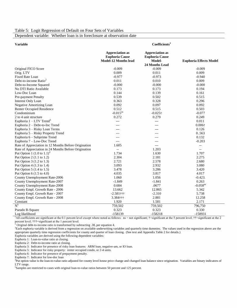
Table 5: Logit Regression of Default on Four Sets of Variables

Dependent variable: Whether loan is in foreclosure at observation date

Variable

Coefficients1

Appreciation as

Euphoria Cause

Model-12 Months lead

Appreciation as

Euphoria Cause

Model-

24 Months Lead

Euphoria Effects Model

Original FICO Score -0.009 -0.009 -0.009

Orig. LTV 0.009 0.011 0.009

Fixed Rate Loan -0.977 -0.973 -0.940

Debt-to-income Ratio2 0.011 0.010 0.009

Debt-to-Income Squared -0.000 -0.000 -0.000

No DTI Ratio Available 0.173 0.173 0.194

Low-Doc Loan 0.144 0.139 0.161

Pre-payment Penalty 0.539 0.502 0.515

Interest Only Loan 0.363 0.328 0.296

Negative Amortizing Loan 0.092 0.097 0.092

Renter Occupied Residence 0.512 0.515 0.503

Condominium -0.015ns -0.025† -0.077

2 to 4 unit structure 0.272 0.279 0.249

Euphoria 1 – LTV Trend3 --- --- 0.011

Euphoria 2 – Debt-to-Inc Trend --- --- 0.006†

Euphoria 3 – Risky Loan Terms --- --- 0.126

Euphoria 5 – Risky Property Trend --- --- 0..563

Euphoria 6 – Subprime Trend --- --- 0.132

Euphoria 7 – Low-Doc Trend --- --- -0.203

Rate of Appreciation in 12 Months Before Origination 1.605 --- --

Rate of Appreciation in 24 Months Before Origination -- 1.203 --

Put Option 1 (1.0 to 1.1)4 1.734 1.630 1.707

Put Option 2 (1.1 to 1.2) 2.304 2.181 2.275

Put Option 3 (1.2 to 1.3) 2.721 2.578 2.680

Put Option 4 (1.3 to 1.4) 3.093 2.932 3.080

Put Option 5 (1.4 to 1.5) 3.478 3.286 3.420

Put Option 6 (1.5 to 4.0) 4.035 3.817 4.017

County Unemployment Rate-2006 1.060 1.056 -0.423.

County Unemployment Rate-2007 -1.849 -1.841 0.263

County Unemployment Rate-2008 0.684 .0677 -0.058ns

County Empl. Growth Rate - 2006 13.662 12.865 5.342

County Empl. Growth Rate - 2007 -2.581††† -2.310 5.738

County Empl. Growth Rate - 2008 3.384††† 2.881 12.258

Constant 1.920 1.581 2.171

N5

Pseudo R-Square

Log likelihood

759,502

0.323

-158139

759,502

0.323

-158218

796,750

0.330

-158931 1All coefficients are significant at the 0.1 percent level except where noted as follows: ns = not significant; †=significant at the 5 percent level; ††=significant at the 2

percent level; †††=significant at the 1 percent level. 2 Original debt-to-income ratio is transformed by subtracting .38, per equation 4. 3Each euphoria variable is derived from a regression on available underwriting variables and quarterly time dummies. The values used in the regression above are the

appropriate quarterly time regression coefficients for county and quarter of loan closing. (See text and Appendix Table 2 for details.)

Euphoria variables are derived using the following dependent variables: Euphoria 1: Loan-to-value ratio at closing.

Euphoria 2: Debt-to-income ratio at closing.

Euphoria 3: Indicator for presence of risky loan features: ARM loan, negative-am, or IO loan. Euphoria 5: Indicator for risky property: renter occupied condo, or 2-4 units.

Euphoria 6: Indicator for presence of prepayment penalty.

Euphoria 7: Indicator for low-doc loan 4Put option value is the loan-to-value ratio adjusted for county level house price change and changed loan balance since origination. Variables are binary indicators of

LTV range. 5Samples are restricted to cases with original loan-to-value ratios between 50 percent and 125 percent.


39

Table 6: Pseudo R2 for Various Nested Sub-models

Pseudo R2

Variables Omitted Model 1 Model 2 Model 3

12 Month Causal 24 Month Causal Euphoria Effects

Full Model (No variables omitted) 32.33 32.30 33.00

Negative Amortization Loan 32.33 32.29 32.99

―Low Doc‖ Loan 32.31 32.28 32.98

Property Type: Condo or 2 to 4 Units 32.32 32.29 32.98

Original Debt-to-Income Ratio 32.27 32.24 32.93

Interest Only Loan 32.18 32.17 32.90

Local Unemployment and Growth 32.03 32.01 32.68

Renter Occupied 32.12 32.08 32.79

Prepayment Penalty 31.39 31.95 32.64

Original LTV 32.29 32.20 32.94

Pre Origination Appreciation 32.24 32.24

Fixed-rate Loan 31.13 31.11 31.90

FICO Score 28.85 33.95 29.56

Put Variables 22.04 23.43 25.01

Euphoria Variables 32.24

All differences from the full model in pseudo-R2 are statistically significant at the 0.1 percent level or higher.


40

Table 7: Effect on Log Odds Ratio from House Price Changes

Effect of a one basis point change in value index*

Euphoria Proxies

Model 1: Appreciation 12 months prior to origination 0.016

Model 2: Appreciation 24 months prior to origination 0.012

Model 3: Combined ―effect‖ proxies 0.007

Put Effects

Model 1 Increase in value index -0.101

Decrease in value index -0.164

Model 2 Increase in value index -0.095 Decrease in value index -0.155 Model 3 Increase in value index -0.099

Decrease in value index -0.160

*Estimates for euphoria proxies, models 1 and 2 are the coefficients of logit regression (Table 5) multiplied by 0.01.

Estimate for euphoria proxy, model 3 is the sum of logit regression coefficients (Table 5), each multiplied by the

marginal effect of change in the house price index (from Table 4). This sum is multiplied by 0.01. Put effects values

are derived by shifting the distribution of estimated loan-to-value ratios across coefficient ―buckets‖ (Table 5) in

response to a one basis point change in the house price index. The difference in the ―bucket‖ weighted average of

the coefficients before and after the change is the effect on the log odds ratio of default.


41

Appendix Table 1

Appreciation Characteristics and Default Incidence by County*

Mean Rate of

Appreciation

1997-2007

Standard

Deviation of

Appreciation

Default

All Counties ---- ---- 8.2

Alachua 2.31 4.10 2.3

Brevard 2.52 4.24 6.5

Collier 1.86 4.37 8.9

Duval 2.25 3.29 5.5

Hernando 2.20 5.33 8.9

Hillsborough 2.27 3.51 7.8

Lake 2.22 3.04 6.3

Lee 2.22 4.61 15.9

Manatee 2.54 3.41 7.9

Martin 2.34 3.44 4.7

Miami-Dade 2.44 4.50 10.2

Orange 2.22 3.08 9.0

Osceola 2.40 3.92 13.5

Palm Beach 2.54 2.80 7.3

Pasco 2.25 2.71 8.1

Pinellas 2.42 3.20 6.2

St. Lucie 2.84 5.43 12.9

Sarasota 2.26 3.80 8.7

Seminole 2.39 3.20 5.4

Volusia 2.40 3.88 6.5 * Appreciation data from authors’ price index. Default data from data of LPS Applied Analytics


42

Appendix Table 2: Aggregate Euphoria Variables and Aggregate House Price Index

Quarter

LTV

Trend

DTI

Trend

Risky

Loan

Trend

Alt-A/

Subprime

Trend

Risky

Property

Trend

Prepayment

Penalty

Trend

Lo-Doc

Trend

House

Price

Index 2001.1 0 0 0 0 0 0 0 1

2001.2 -2.161 -0.271 0.160 0.007 0.140 -0.014 -0.059 1.031

2001.3 -1.536 0.430 0.269 -0.010 0.507 0.173 -0.155 1.051

2001.4 -4.821 -0.266 0.114 0.164 0.216 0.149 -0.158 1.074

2002.1 -4.160 0.185 0.923 -0.113 0.605 0.239 -0.452 1.094

2002.2 -3.768 0.410 0.904 -0.262 0.755 -0.299 -0.386 1.136

2002.3 -6.183 -0.986 0.751 -0.236 0.376 -0.506 -0.641 1.166

2002.4 -8.302 -1.046 0.680 -0.082 0.421 -0.705 -0.645 1.191

2003.1 -9.452 2.469 1.181 -0.023 0.597 -0.253 -0.735 1.221

2003.2 -10.660 2.249 1.285 0.128 0.750 -0.130 -0.742 1.261

2003.3 -12.333 1.971 1.630 0.287 0.701 0.366 -0.672 1.300

2003.4 -8.032 1.952 2.111 0.433 0.889 0.482 -0.311 1.353

2004.1 -8.732 1.003 2.355 0.524 0.962 0.916 -0.466 1.397

2004.2 -8.911 1.714 2.771 0.555 1.043 0.999 -0.444 1.469

2004.3 -6.062 1.915 2.919 0.654 1.141 1.081 -0.205 1.556

2004.4 -7.086 3.081 3.045 0.855 1.174 1.346 -0.151 1.620

2005.1 -6.586 3.294 3.116 1.010 1.310 1.578 -0.068 1.729

2005.2 -6.453 3.021 3.317 1.074 1.326 1.887 -0.141 1.869

2005.3 -8.709 3.543 3.204 1.082 1.366 1.981 -0.171 2.015

2005.4 -9.270 3.747 3.295 0.971 1.207 1.891 -0.233 2.137

2006.1 -9.161 3.392 3.347 0.866 1.024 1.680 -0.124 2.279

2006.2 -8.356 3.815 3.320 1.111 0.944 2.015 -0.061 2.347

2006.3 -9.313 3.675 3.379 1.094 0.861 2.022 -0.127 2.390

2006.4 -10.182 3.090 3.269 1.163 0.948 2.100 -0.114 2.382

2007.1 -10.266 3.562 3.071 0.986 0.912 1.874 -0.140 2.173

2007.2 -8.917 4.939 2.707 0.719 0.778 1.445 -0.078 2.151

2007.3 -7.180 4.967 2.490 0.586 0.587 1.112 0.087 2.043

2007.4 -5.960 5.208 1.725 0.233 0.776 0.182 -0.042

A quick review of the aggregate euphoria variables above illuminates clear trends tied to the events in the market.

Consider the risky loan trend and the prepayment penalty trend. Both are increasing as the index moves up and then

begins to decrease in much the same fashion as the trend near the end of 2007.

Working Paper Series - Richmond Fed/media/richmondfedorg/publications/... · Volatility, Euphoria...

Documents

Transcript of Working Paper Series - Richmond Fed/media/richmondfedorg/publications/... · Volatility, Euphoria...