Working Paper Series - ecb.europa.eu label these models SW, SWFF and SWU, respectively. ......
101
Working Paper Series Euro area real-time density forecasting with financial or labor market frictions Peter McAdam, Anders Warne Disclaimer: This paper should not be reported as representing the views of the European Central Bank (ECB). The views expressed are those of the authors and do not necessarily reflect those of the ECB. No 2140 / April 2018
Transcript of Working Paper Series - ecb.europa.eu label these models SW, SWFF and SWU, respectively. ......

Working Paper Series Euro area real-time density forecasting with financial or labor market frictions
Peter McAdam, Anders Warne
Disclaimer: This paper should not be reported as representing the views of the European Central Bank (ECB). The views expressed are those of the authors and do not necessarily reflect those of the ECB.
No 2140 / April 2018

Abstract: We compare real-time density forecasts for the euro area using three DSGE models.
The benchmark is the Smets-Wouters model and its forecasts of real GDP growth and inflation
are compared with those from two extensions. The first adds financial frictions and expands
the observables to include a measure of the external finance premium. The second allows for
the extensive labor-market margin and adds the unemployment rate to the observables. The
main question we address is if these extensions improve the density forecasts of real GDP and
inflation and their joint forecasts up to an eight-quarter horizon. We find that adding financial
frictions leads to a deterioration in the forecasts, with the exception of longer-term inflation
forecasts and the period around the Great Recession. The labor market extension improves
the medium to longer-term real GDP growth and shorter to medium-term inflation forecasts
weakly compared with the benchmark model.
Keywords: Bayesian inference, DSGE models, forecast comparison, inflation, output, predic-
tive likelihood.
JEL Classification Numbers: C11, C32, C52, C53, E37.
ECB Working Paper Series No 2140 / April 2018 1

Non-Technical Summary
Medium-size dynamic stochastic general equilibrium (DSGE) models—as exemplified by Smets
and Wouters (2007)—have been widely used among central banks for policy analysis, forecast-
ing and to provide a structural interpretation of economic developments; see, e.g., Del Negro
and Schorfheide (2013) and Lindé, Smets, and Wouters (2016). Recent years have, however,
constituted an especially challenging policy environment. Given the global financial crisis in
late 2008, the Great Recession that followed, and the European sovereign debt crisis starting in
late 2009, many economies witnessed sharp falls in activity and inflation, persistent increases
in unemployment, and widening financial spreads. In such a severe downturn, large forecasts
errors may be expected across all models.
In the case of DSGE models, two prominent criticisms additionally emerged: (i) that such
models were lacking ‘realistic’ features germane to the crisis, namely financial frictions and
involuntary unemployment; and (ii) that their strong equilibrium underpinnings made them
vulnerable to forecast errors following a severe, long-lasting downturn. For such debates see,
inter alia, Caballero (2010), Hall (2010), Ohanian (2010), Buch and Holtemöller (2014) and
Lindé et al. (2016).
In this paper we compare real-time density forecasts for the euro area based on three estimated
DSGE models. The benchmark is that of Smets and Wouters (2007), as adapted to the euro
area, and its real-time forecasts of real GDP growth and inflation. These forecasts are compared
with those from two extensions of the model. The first adds the financial accelerator mecha-
nism of Bernanke, Gertler, and Gilchrist (1999) (BGG) and augments the list of observables to
include a measure of the external finance premium. The second allows for an extensive labor
margin, following Galí (2011) and Galí, Smets, and Wouters (2012), and, likewise, augments
the unemployment rate to the set of observables. We label these models SW, SWFF and SWU,
respectively. The euro area real-time database (RTD), on which these models are estimated and
assessed, is described in Giannone, Henry, Lalik, and Modugno (2012). To extend the data back
in time, we follow Smets, Warne, and Wouters (2014) and link the real-time data to various
updates from the area-wide model (AWM) database; see Fagan, Henry, and Mestre (2005).
Against this background, we strive to make the following contributions. First, we report the
density forecasting of the SW model and the two model variants, SWFF and SWU, over a period
prior to and after the more recent crises; namely, 2001–2014. These additional variants, reflect
‘missing’ elements emphasized by some critics of the core model: namely, financial frictions,
and ‘extensive’ labor-market modelling. The importance of combining models for predictive
and policy-analysis purposes is an enduring topic in the literature, see e.g., Levine, McAdam,
and Pearlman (2008), Geweke and Amisano (2011), or Amisano and Geweke (2017). In that
respect, it is important to compare sufficiently differentiated models, to balance different and
relevant economic mechanisms. Indeed, although the BGG extension to the core model has
been much discussed, that allowing for extensive employment fluctuations has received less
ECB Working Paper Series No 2140 / April 2018 2

attention. And yet, we know that unemployment was high by international comparisons in
many euro area economies prior to the crisis, and slow to revert back to pre-crisis levels thereafter
(European Commission, 2016). It is of interest therefore to assess the forecasting contribution
of models which attempted to capture extensive fluctuations over the crisis. To our knowledge,
this is the first time these three models have been estimated on a common basis and directly
compared with an emphasis on their density forecasting comparisons. Accordingly, we can
address the question of whether these extensions did or can improve the density forecasts of
growth and inflation and their joint forecasts.
Our second contribution is that we focus on real-time forecasting performance. It has be-
come standard to use real-time data when analyzing the out-of-sample forecast performances of
competing models. In our exercises, we utilize the euro area RTD. It is also worth noting that
forecasting applications of the RTD for the euro area have been relatively few. An important
exception is Smets et al. (2014), who also use the SWU model for real-time analysis, and other
examples are Conflitti, De Mol, and Giannone (2015), Jarociński and Lenza (2016) and Pirschel
(2016). In view of the limited number of studies based on real-time euro area data, our paper
can therefore be seen as building on and extending this important line of research.
Turning to our results, we note the following. Regarding the point forecasts based on the
predictive mean, all models over-predict GDP growth over most of the sample, and in particular
beyond 2009. The SWFF model has the largest (if most stable) forecast errors relative to SW
and SWU, which are both relatively similar. Concerning the inflation forecasts the SWFF model
under-predicts and especially at the shorter horizons while the SW and SWU models perform
similarly with a tendency to over-predict at the longer horizons. In that regard, we concur with
Kolasa and Rubaszek (2015) that a model with the basic financial accelerator mechanism is
(in forecasting terms) not an obviously superior alternative. For a more detailed discussion of
different modelling and methodological approaches to take in the wake of the crisis to improve
models, see Lindé et al. (2016).
In terms of the density forecasts, where the predictive density evaluated at the actual outcome
is used to compare models, we also find that the SW and SWU models yield similar density
forecasts and dominate the SWFF model. Since the onset of the crisis there is a tendency for
the SWU model to forecast better over the medium term, while the SW model tends to dominate
weakly over the shorter term. All models display a drop in performance with the onset of the
crisis in 2008Q4 and 2009Q1. At the same time, this drop looks like a one-time event and the
ability of the models have otherwise not been notably affected.
ECB Working Paper Series No 2140 / April 2018 3

1. Introduction
Medium-size dynamic stochastic general equilibrium (DSGE) models—as exemplified by Smets
and Wouters (2007)—have been widely used among central banks for policy analysis, forecasting
and to provide a structural interpretation of economic developments; see, e.g., Del Negro and
Schorfheide (2013) and Lindé et al. (2016). Recent years have, however, constituted an especially
challenging policy environment. Given the global financial crisis in late 2008, the Great Reces-
sion that followed, and the European sovereign debt crisis starting in late 2009, many economies
witnessed sharp falls in activity and inflation, persistent increases in unemployment, and widen-
ing financial spreads. In such a severe downturn, large forecasts errors may be expected across
all models.
In the case of DSGE models, two prominent criticisms additionally emerged: (i) that such
models were lacking ‘realistic’ features germane to the crisis, namely financial frictions and
involuntary unemployment; and (ii) that their strong equilibrium underpinnings made them
vulnerable to forecast errors following a severe, long-lasting downturn. For such debates see,
inter alia, Caballero (2010), Hall (2010), Ohanian (2010), Buch and Holtemöller (2014) and
Lindé et al. (2016).
In this paper we compare real-time density forecasts for the euro area based on three estimated
DSGE models. The benchmark is that of Smets and Wouters (2007), as adapted to the euro
area, and its real-time forecasts of real GDP growth and inflation. These forecasts are compared
with those from two extensions of the model. The first adds the financial accelerator mechanism
of Bernanke et al. (1999) (BGG) and augments the list of observables to include a measure
of the external finance premium. The second allows for an extensive labor margin, following
Galí (2011) and Galí et al. (2012), and, likewise, augments the unemployment rate to the set of
observables. We label these models SW, SWFF and SWU, respectively. The euro area real-time
database (RTD), on which these models are estimated and assessed, is described in Giannone
et al. (2012). To extend the data back in time, we follow Smets et al. (2014) and link the
real-time data to various updates from the area-wide model (AWM) database; see Fagan et al.
(2005).
More generally, while financial frictions had already been introduced into some estimated
DSGE models prior to the financial crisis, such extensions of the ‘core’ model were not yet
standard; see, e.g., Christiano, Motto, and Rostagno (2003, 2008) and De Graeve (2008). Since
the crisis there has been an active research agenda exploring extensions to the core model. For
instance, Lombardo and McAdam (2012) considered the inclusion of the financial accelerator
on firms’ financing side alongside constrained and unconstrained households; see also Kolasa,
Rubaszek, and Skrzypczyński (2012). Del Negro and Schorfheide (2013) also integrated the effect
of BGG financial frictions on the core (SW) model and compared its forecasting performance
with non model-based ones. Moreover, Christiano, Trabandt, and Walentin (2011) considered
ECB Working Paper Series No 2140 / April 2018 4

the open-economy dimension to financial frictions in a somewhat larger-scale model, which also
included labor market frictions.
However, in terms of forecasting performance and model fit, it is by no means clear whether
these extensions have improved matters. For instance, while Del Negro and Schorfheide (2013)
and Christiano et al. (2011) favorably report the forecasting performance of the SW model aug-
mented by financial frictions, Kolasa and Rubaszek (2015) find that adding financial frictions can
worsen the average quality of density forecasts, depending on the friction examined. Moreover,
while Del Negro and Schorfheide (2013) use (US) real time data, the other two studies do not.
Nor is there a common basis of forecast comparison across these papers: Kolasa and Rubaszek
(2015) and Del Negro and Schorfheide (2013) emphasize density forecasts, whereas Christiano
et al. (2011) use point forecasts.
Against this background, we strive to make the following contributions. First, we report the
density forecasting of the SW model and the two model variants, SWFF and SWU, over a period
prior to and after the more recent crises; namely, 2001–2014. These additional variants, reflect
‘missing’ elements emphasized by some critics of the core model: namely, financial frictions,
and ‘extensive’ labor-market modelling. The importance of combining models for predictive and
policy-analysis purposes is an enduring topic in the literature, see e.g., Levine et al. (2008),
Geweke and Amisano (2011), or Amisano and Geweke (2017). In that respect, it is important
to compare sufficiently differentiated models, to balance different and relevant economic mech-
anisms. Indeed, although the BGG extension to the core model has been much discussed, that
allowing for extensive employment fluctuations has received less attention. And yet, we know
that unemployment was high by international comparisons in many euro area economies prior to
the crisis, and slow to revert back to pre-crisis levels thereafter (European Commission, 2016).
It is of interest therefore to assess the forecasting contribution of models which attempted to
capture extensive fluctuations over the crisis. To our knowledge, this is the first time these
three models have been estimated on a common basis and directly compared with an emphasis
on their density forecasting comparisons. Accordingly, we can address the question of whether
these extensions did or can improve the density forecasts of growth and inflation and their joint
forecasts.
Our second contribution is that we focus on real-time forecasting performance. It has be-
come standard to use real-time data when analyzing the out-of-sample forecast performances of
competing models. In our exercises, we utilize the euro area RTD. It is also worth noting that
forecasting applications of the RTD for the euro area have been relatively few. An important
exception is Smets et al. (2014), who also use the SWU model for real-time analysis, and other
examples are Conflitti et al. (2015), Jarociński and Lenza (2016) and Pirschel (2016). In view
of the limited number of studies based on real-time euro area data, our paper can therefore be
seen as building on and extending this important line of research.
ECB Working Paper Series No 2140 / April 2018 5

The paper is organized as follows. Section 2 provides sketches of the three DSGE models. Prior
distributions of the parameters are discussed in Section 3, while the full sample set of posteriors,
impulse responses and forecast error variance decompositions are covered in Section 4.1 The
RTD of the euro area is the main topic in Section 5, along with how this data is linked backward
in time with various updates of the AWM database. Section 6 contains the empirical results on
point and density forecasts of real GDP growth and GDP deflator inflation, including backcasts,
nowcasts, and one-quarter-ahead up to eight-quarter-ahead forecasts. Section 7 summarizes the
main findings, while a detailed exposition of the DSGE models is provided in the Appendix.
2. The Models
In this section, we sketch the three models. The baseline model is that of Smets and Wouters
(2007), where the authors study shocks and frictions in US business cycles. To this we add two
augmented models: a version with an external finance premium, and one with the modelling
of an extensive employment margin. The Appendix describes the frameworks in greater detail
including a treatment of their flexible price and wage analogues, and their steady state equations.
2.1. SW Model Equations
The log-linearized aggregate resource constraint of this closed economy model is given by
yt = cy ct + iy it + zyzt + εgt , (1)
where yt is (detrended) real GDP. It is absorbed by real private consumption (ct), real private
investments (it), the capital utilization rate (zt), and exogenous spending (εgt ). The parameter
cy is the steady-state consumption-output ratio and iy is the steady-state investment-output
ratio, where
cy = 1 − iy − gy,
and gy is the steady-state exogenous spending-output ratio. The steady-state investment-output
ratio is determined by
iy = (γ + δ − 1) ky,
where ky is the steady-state capital-output ratio, γ is the steady-state growth rate, and δ is the
depreciation rate of capital. Finally,
zy = rkky,
where rk is the steady-state rental rate of capital. The steady-state parameters are shown in
Section A.5, but it is noteworthy already at this stage that zy = α, the share of capital in
production.
The dynamics of consumption follows from the consumption Euler equation and is equal to
ct = c1ct−1 + (1 − c1)Etct+1 + c2
(lt − Et lt+1
)− c3
(rt − Etπt+1
)+ εbt , (2)
1The full sample is given by update 14 of the AWM database, covering the period 1980Q1–2013Q4.
ECB Working Paper Series No 2140 / April 2018 6

where lt is hours worked, rt is the policy controlled nominal interest rate, and εbt is proportional
to the exogenous risk premium, i.e., a wedge between the interest rate controlled by the central
bank and the return on assets held by households. It should be noted that in contrast to Smets
and Wouters (2007), but identical to Smets and Wouters (2005) and Lindé et al. (2016), we have
moved the risk premium variable outside the expression for the ex ante real interest rate. This
means that εbt = −c3εbt , where εbt is the risk premium variable in Smets and Wouters (2007).
Building on the work by Krishnamurthy and Vissing-Jorgensen (2012), Fisher (2015) shows
that this shock can be given a structural interpretation, namely, as a shock to the demand for
safe and liquid assets or, alternatively, as a liquidity preference shock. The parameters of the
consumption Euler equation are:
c1 =λ/γ
1 + (λ/γ), c2 =
(σc − 1) (whl/c)σc (1 + (λ/γ))
, c3 =1 − (λ/γ)
σc (1 + (λ/γ)),
where λ measures external habit formation, σc is the inverse of the elasticity of intertemporal
substitution for constant labor, while whl/c is the steady-state hourly real wage bill to consump-
tion ratio. If σc = 1 (log-utility) and λ = 0 (no external habit) then the above equation reduces
to the familiar purely forward looking consumption Euler equation.
The log-linearized investment Euler equation is given by
it = i1 it−1 + (1 − i1)Etit+1 + i2qt + εit, (3)
where qt is the real value of the existing capital stock, while εit is an exogenous investment-specific
technology variable. The parameters of (3) are given by
i1 =1
1 + βγ1−σc, i2 =
1(1 + βγ1−σc) γ2ϕ
,
where β is the discount factor used by households, and ϕ is the steady-state elasticity of the
capital adjustment cost function.
The dynamic equation for the value of the capital stock is
qt = q1Etqt+1 + (1 − q1)Etrkt+1 −(rt − Etπt+1
)+ c−1
3 εbt , (4)
where rkt is the rental rate of capital. The parameter q1 is here given by
q1 = βγ−σc(1 − δ) =1 − δ
rk + 1 − δ.
Turning to the supply-side of the economy, the log-linearized aggregate production function
can be expressed as
yt = φp
[αkst + (1 − α) lt + εat
], (5)
where kst is capital services used in production, and εat an exogenous total factor productivity
variable. As mentioned above, the parameter α reflects the share of capital in production, while
φp is equal to one plus the steady-state share of fixed costs in production.
ECB Working Paper Series No 2140 / April 2018 7

The capital services variable is used to reflect that newly installed capital only becomes
effective with a one period lag. This means that
kst = kt−1 + zt, (6)
where kt is the installed capital. The degree of capital utilization is determined from cost
minimization of the households that provide capital services and is therefore a positive function
of the rental rate of capital. Specifically,
zt = z1rkt , (7)
where z1 =1 − ψ
ψand ψ is a positive function of the elasticity of the capital adjustment cost
function and normalized to lie between 0 and 1. The larger ψ is the costlier it is to change
the utilization of capital. The log-linearized equation that specifies the development of installed
capital is
kt = k1kt−1 + (1 − k1) it + k2εit. (8)
where k1 =1 − δ
γand k2 = (γ + δ − 1)
(1 + βγ1−σc
)γϕ.
From the monopolistically competitive goods market, the price markup (µpt ) is equal to minus
the real marginal cost (µct) under cost minimization by firms. That is,
µpt = α(kst − lt
)− wt + εat , (9)
where the real wage is given by wt. Similarly, the real marginal cost is
µct = αrkt + (1 − α) wt − εat , (10)
where (10) is obtained by substituting for the optimally determined capital-labor ratio in equa-
tion (12).
Due to price stickiness, and partial indexation to lagged inflation of those prices that cannot
be re-optimized, prices adjust only sluggishly to their desired markups. Profit maximization by
price-setting firms yields the log-linearized price Phillips curve,
πt = π1πt−1 + π2Etπt+1 − π3µpt + εpt
= π1πt−1 + π2Etπt+1 + π3µct + εpt ,
(11)
where εpt is an exogenous price markup process. The parameters of the Phillips curve are given
by
π1 =ıp
1 + βγ1−σc ıp, π2 =
βγ1−σc
1 + βγ1−σc ıp, π3 =
(1 − ξp)(1 − βγ1−σcξp
)(1 + βγ1−σc ıp) ξp ((φp − 1)εp + 1)
.
The degree of indexation to past inflation is determined by the parameter ıp, ξp measures the
degree of price stickiness such that 1− ξp is the probability that a firm can re-optimize its price,
and εp is the curvature of the Kimball (1995) goods market aggregator.
ECB Working Paper Series No 2140 / April 2018 8

Cost minimization of firms also implies that the rental rate of capital is related to the capital-
labor ratio and the real wage according to.
rkt = −(kst − lt
)+ wt. (12)
In the monopolistically competitive labor market the wage markup is equal to the difference
between the real wage and the marginal rate of substitution between labor and consumption
µwt = wt −(σl lt +
11 − (λ/γ)
[ct − λ
γct−1
]), (13)
where σl is the elasticity of the labor input with respect to real wages.
Due to wage stickiness and partial wage indexation, real wages respond gradually to the
desired wage markup
wt = w1wt−1 + (1 − w1)[Etwt+1 + Etπt+1
]− w2πt + w3πt−1 − w4µwt + εwt , (14)
where εwt is an exogenous wage markup process. The parameters of the wage equation are
w1 =1
1 + βγ1−σc, w2 =
1 + βγ1−σc ıw1 + βγ1−σc
,
w3 =ıw
1 + βγ1−σc, w4 =
(1 − ξw)(1 − βγ1−σcξw
)(1 + βγ1−σc) ξw ((φw − 1) εw + 1)
.
The degree of wage indexation to past inflation is given by the parameter ıw, while ξw is the
degree of wage stickiness. The steady-state labor market markup is equal to φw − 1 and εw is
the curvature of the Kimball labor market aggregator.
The sticky price and wage part of the model is closed by adding the monetary policy reaction
function
rt = ρrt−1 + (1 − ρ)[rππt + ry
(yt − yft
)]+ r∆y
[∆yt − ∆yft
]+ εrt , (15)
where yft is potential output measured as the level of output that would prevail under flexible
prices and wages in the absence of the two exogenous markup processes, whereas εrt is an
exogenous monetary policy shock process.
As productivity is written in terms of hours worked, we introduce an auxiliary equation with
Calvo-rigidity to link from observed total employment (et) to unobserved hours worked:
et − et−1 = β(Etet+1 − et
)+
(1 − βξe
)(1 − ξe
)ξe
(lt − et
), (16)
where 1− ξe is the fraction of firms that are able to adjust employment to its desired total labor
input; see Adolfson, Laséen, Lindé, and Villani (2005, 2007a).
2.1.1. The Exogenous Variables
There are seven exogenous processes in the Smets and Wouters (2007) model. These are generally
modelled as AR(1) process with the exception of the exogenous spending process (where the
process depends on both the exogenous spending shock ηgt and the total factor productivity
ECB Working Paper Series No 2140 / April 2018 9

shock ηat ) and the exogenous price and wage markup processes, which are treated as ARMA(1,1)
processes. This means that
εat = ρaεat−1 + σaη
at ,
εbt = ρbεbt−1 + σbη
bt ,
εgt = ρgεgt−1 + σgη
gt + ρgaσaη
at ,
εit = ρiεit−1 + σiη
it,
εpt = ρpεpt−1 + σpη
pt − µpσpη
pt−1,
εrt = ρrεrt−1 + σrη
rt ,
εwt = ρwεwt−1 + σwη
wt − µwσwη
wt−1.
(17)
The shocks ηjt , j = {a, b, g, i, p, r, w}, are N(0, 1), where ηbt is a preference shock (proportional
to a risk premium shock), ηit is an investment-specific technology shock, ηpt is a price markup
shock, ηrt is a monetary policy or interest rate shock, and ηwt is a wage markup shock.
2.2. The SWFF Model
Lombardo and McAdam (2012) and Del Negro and Schorfheide (2013) introduce financial fric-
tions into variants of the SW model based on the financial accelerator approach of Bernanke
et al. (1999); see also Christiano et al. (2003, 2008) and De Graeve (2008). This amounts to
replacing the value of the capital stock equation in (4) with
Etret+1 − rt = ζsp,b
(qt + kt − nt
)− c−13 εbt + εet , (18)
and
ret − πt =(1 − q1
)rkt + q1qt − qt−1, (19)
where ret is the gross return on capital for entrepreneurs, nt is entrepreneurial equity (net worth),
and εet captures mean-preserving changes in the cross-sectional dispersion of ability across en-
trepreneurs, a spread shock. The parameter q1 is here given by
q1 =1 − δ
rk + 1 − δ,
where rk is generally not equal to β−1γσc + δ − 1 since the spread between gross returns on
capital for entrepreneurs and the nominal interest rate need not equal zero. The spread shock
is assumed to follow the AR(1) process
εet = ρeεet−1 + σeη
et . (20)
The parameters ζsp,b is the steady-state elasticity of the spread with respect to leverage. It may
be noted that if ζsp,b = σe = 0, then the financial frictions are shut down and equations (18)
and (19) yield the original value of the capital stock equation (4).
ECB Working Paper Series No 2140 / April 2018 10

The log-linearized net worth of entrepreneurs equation is given by
nt = ζn,e(ret − πt
)− ζn,r(rt−1 − πt
)+ ζn,q
(qt−1 + kt−1
)+ ζn,nnt−1 − ζn,σω
ζsp,σω
εet−1, (21)
where ζn,e, ζn,r, ζn,q, ζn,n, and ζn,σω are the steady-state elasticities of net worth with respect to
the return on capital for entrepreneurs, the interest rate, the cost of capital, lagged net worth,
and the volatility of the spread shock. Furthermore, ζsp,σω is the steady-state elasticity of the
spread with respect to the spread shock. Expressions for these elasticities are given in Appendix
Section A.10.
2.3. The SWU Model
The Galí, Smets, and Wouters (2012, GSW) model is an extension of the standard SW model
which explicitly provides a mechanism for explaining unemployment. This is accomplished by
modelling the labor supply decisions on the extensive margin (whether to work or not) rather
than on the intensive margin (how many hours to work). As a consequence, the unemployment
rate is added as an observable variable, while labor supply shocks are admitted. This allows the
authors to overcome the lack of identification of wage markup and labor supply shocks raised
by Chari, Kehoe, and McGrattan (2009) in their critique of new Keynesian models. From a
technical perspective the GSW model is also based on the assumption of log-utility, i.e. the
parameter σc is assumed to be unity, but the equations presented below will instead be written
as if this is a free parameter and therefore treat σc as in Section A.1 and A.7.
Smets, Warne, and Wouters (2014) present a variant of the GSW model aimed for the euro
area and this version is presented below. The log-linearized aggregate resource constraint is
given by equation (1). The consumption Euler equation may be expressed as
λt = Etλt+1 +(rt − Etπt+1
)− c−13 εbt , (22)
where λt is the log-linearized marginal utility of consumption, given by
λt = − σc1 − (λ/γ)
[ct − λ
γct−1
]+
(σc − 1)(whl/c)1 − (λ/γ)
lt, (23)
while εbt is the preference shock. Making use of (22) and (23), the consumption Euler equation
can be written in the more familiar form in equation (2), and where c3 is given by the expressions
below this equation. However, below we have use for the expression for λt.
Concerning the Phillips curve, it is similar to equation (11), but differs in the way that the
price markup shock enters the model:
πt = π1πt−1 + π2Etπt+1 − π3
(µpt − µn,pt
). (24)
The expressions for πi below equation (11) hold and the natural price markup shock µn,pt = 100εpt .
The average price markup and the real marginal cost variables are given by equation (9) and
(10), respectively. Relative to equation (11), the price markup shock εpt = π3100εpt . Smets,
ECB Working Paper Series No 2140 / April 2018 11

Warne, and Wouters (2014) uses the shock εpt , while we wish to treat the price markup shock
symmetrically in the three models and therefore keep equation (11) such that our price markup
shock is given by εpt .
In the GSW model, the wage Phillips curve in equation (14) is replaced with the following
expression for real wages
wt = w1wt−1 + (1 − w1)[Etwt+1 + Etπt+1
]− w2πt + w3πt−1 − w4
[µwt − µn,wt
], (25)
where µwt is the average wage markup and µn,wt is the natural wage markup. Notice that the wiparameters are given by the expressions below equation (14) for i = 1, 2, 3, while
w4 =
(1 − ξw
)(1 − βγ1−σcξw
)(1 + βγ1−σc
)ξw(1 + εwσl
) .In addition, GSW and Smets, Warne, and Wouters (2014) let the curvature of the Kimball labor
market aggregator be given by εw =φw
φw − 1.
The average wage markup is defined as the difference between the real wage and the marginal
rate of substitution, which is a function of the adjusted smoothed trend in consumption, xt,
the marginal utility of consumption λt, total employment, et, and the labor supply shock. This
expression is equal to the elasticity of labor supply times the unemployment rate, i.e.
µwt = σlut
= wt −(xt − λt + εst + σlet
),
(26)
where unemployment is defined as labor supply minus total employment:
ut = lst − et. (27)
The labor supply shock is assumed to follow an AR(1) process such that
εst = ρsεst−1 + σsη
st . (28)
The natural wage markup shock is expressed as 100εwt and is, in addition, equal to the elasticity
of labor supply times the natural rate of unemployment. Accordingly,
µn,wt = 100εwt = σlunt . (29)
The natural rate of unemployment, unt , is defined as the unemployment rate that would prevail
in the absence of nominal wage rigidities, and is here proportional to the natural wage markup.
Finally, we here let the wage markup shock, εwt , be defined such that:
εwt = w4µn,wt = w4100εwt .
Hence, the wage markup shock εwt enters equation (25) suitably re-scaled and, apart from the
definition of the w4 parameter, the wage Phillips curve is identical to equation (14). This has
ECB Working Paper Series No 2140 / April 2018 12

the advantage of allowing us to treat the wage markup shock as symmetrically as possible in the
three models.
The adjusted smoothed trend in consumption is given by
xt = κt − 11 − (λ/γ)
[ct − λ
γct−1
], (30)
where the second term on the right hand side is the adjustment, while the smoothed trend in
consumption is given by
κt =(1 − υ
)κt−1 +
υ
1 − (λ/γ)
[ct − λ
γct−1
]. (31)
Making use of equation (23), we find that xt − λt = κt when σc = 1, thereby simplifying the
expression of the average markup in (26). Provided that σc = 1, the parameter υ measures the
weight on the marginal utility of consumption of the smooth trend in consumption. Notice that
if σc = υ = 1 and εst = 0, then the average wage markup in (26) is very similar to the wage
markup in equation (13) of the SW model, with the only difference being that et replaces lt.
2.4. The Measurement Equations
The Smets and Wouters (2007) model is consistent with a balanced steady-state growth path
(BGP) driven by deterministic labor augmenting technological progress. The observed variables
for the euro area are given by quarterly data of the log of real GDP for the euro area (yt),
the log of real private consumption (ct), the log of real total investment (it), the log of total
employment (et), the log of quarterly GDP deflator inflation (πt), the log of real wages (wt), and
the short-term nominal interest rate (rt) given by the 3-month EURIBOR rate. Except for the
nominal interest rate, the natural logarithm of each observable is multiplied by 100 to obtain a
comparable scale. The measurement equations are given by⎡⎢⎢⎢⎢⎢⎢⎢⎢⎢⎢⎢⎢⎢⎢⎢⎢⎢⎢⎣
∆yt
∆ct
∆it
∆wt
∆et
πt
rt
⎤⎥⎥⎥⎥⎥⎥⎥⎥⎥⎥⎥⎥⎥⎥⎥⎥⎥⎥⎦
=
⎡⎢⎢⎢⎢⎢⎢⎢⎢⎢⎢⎢⎢⎢⎢⎢⎢⎢⎢⎣
γ + e
γ + e
γ + e
γ
e
π
4r
⎤⎥⎥⎥⎥⎥⎥⎥⎥⎥⎥⎥⎥⎥⎥⎥⎥⎥⎥⎦
+
⎡⎢⎢⎢⎢⎢⎢⎢⎢⎢⎢⎢⎢⎢⎢⎢⎢⎢⎢⎣
yt − yt−1
ct − ct−1
it − it−1
wt − wt−1
et − et−1
πt
4rt
⎤⎥⎥⎥⎥⎥⎥⎥⎥⎥⎥⎥⎥⎥⎥⎥⎥⎥⎥⎦
. (32)
Since all observed variables except the short-term nominal interest rate (which is already reported
in percent) are multiplied by 100, it follows that the steady-state values on the right hand side
are given by
γ = 100 (γ − 1) , π = 100 (π − 1) , r = 100(
π
βγ−σc− 1),
ECB Working Paper Series No 2140 / April 2018 13

where π is steady-state inflation while e reflects steady-state labor force growth. The interest
rate in the model, rt, is measured in quarterly terms in the model and is therefore multiplied by
4 in (32) to restore it to annual terms for the measurement.
Apart from the steady-state exogenous spending-output ratio only six additional parameters
are calibrated. These are δ = 0.025, φw = 1.5, εp = εw = 10, and µp = µw = 0. The latter two
parameters are estimated by Smets and Wouters (2007) on US data, but we have here opted to
treat all exogenous processes in the model symmetrically. The remaining 20 structural and 15
shock process parameters are estimated. When estimating the parameters, we make use of the
following transformation of the discount factor
β =1
1 +(β/100
) .Following Smets and Wouters (2007), a prior distribution is assumed for the parameter β, while
β is determined from the above equation.
2.4.1. Measurement Equations: SWFF
The set of measurement equations is augmented in Del Negro and Schorfheide (2013) by
st = 4s + 4Et[ret+1 − rt
], (33)
where s is equal to the natural logarithm of the steady-state spread measured in quarterly terms
and in percent, s = 100 ln(re/r), while st is a suitable spread variable. The parameter s is linked
to the steady-state values of the model variable variables according to
re
r= (1 + s/100)1/4 ,
r
π= β−1γσc ,
re
π= rk + 1 − δ.
If there are no financial frictions, then re = r, with the consequence that the steady-state
real interest rate is equal to the steady-state real rental rate on capital plus one minus the
depreciation rate of capital, i.e., the Smets and Wouters steady-state value; see Section A.5.
Del Negro and Schorfheide (2013) estimate s, ζsp,b, ρe, and σe while the parameters F and κe
are calibrated. The latter two parameters will appear in the next Section on the steady-state, but
it is useful to know that they represent the steady-state default probability and survival rate of
entrepreneurs, respectively, with F determined such that in annual terms the default probability
is 0.03 (0.0075 in quarterly terms) and κe = 0.99. These values are also used by Del Negro,
Giannoni, and Schorfheide (2015). Finally, the financial frictions extension also involves the
following calibrated parameters: δ = 0.025, φw = 1.5, εp = εw = 10, and µp = µw = 0.
2.4.2. Measurement Equations: SWU
The steady-state values of the capital-output ratio, etc., are determined as in Section A.5 for the
SW model. The model is consistent with a BGP, driven by deterministic labor augmenting trend
growth, and the vector of observed variables for the euro area is augmented with an equation
ECB Working Paper Series No 2140 / April 2018 14

for unemployment, denoted by ut. Specifically,
ut = u+ ut. (34)
The steady-state parameter u is given by
u = 100(φw − 1σl
), (35)
where (φw − 1) is the steady-state labor market markup and σl is the elasticity of labor supply
with respect to the real wage. Apart from the parameter σc, four additional structural param-
eters are calibrated. These are gy = 0.18, δ = 0.025, and εp = 10 as in the SW model. Unlike
Galí et al. (2012) and Smets et al. (2014) we estimate the persistence parameter of the labor
supply shock, ρs, and calibrate φw = 1.5. The latter parameter can also be estimated and yields
posterior mean and mode estimates very close to 1.5 when using the same prior as in Galí et al.
(2012) and Smets et al. (2014). We have opted to calibrate it in this study in order to treat it
in the same way across the three models.
3. Prior Distributions
The details on the prior distributions of the structural parameters of the three models are listed
in Table 1. For the Smets and Wouters (SW) model and the extension with financial frictions
(SWFF) the prior parameters have typically been selected as in Del Negro and Schorfheide
(2013), where US instead of euro area data are used. In the case of ξe we use the same prior
as in Smets and Wouters (2003) and in Smets et al. (2014). Before we go into further details,
it should be borne in mind that we use exactly the same priors for the models for all data
vintages. Moreover, the priors have been checked with the real-time data vintages to ensure
that the posterior draws are well behaved.
Turning first to the structural parameters, the priors are typically the same across the three
models. One difference is the prior mean and standard deviation of ξp (the degree of price
stickiness) for the SWFF model, which has a higher mean and a lower standard deviation than
in the other two models. The prior standard deviation of ϕ (the steady-state elasticity of the
capital adjustment cost function) is unity in Galí et al. (2012) and Smets et al. (2014) while it
is 1.5 in Del Negro and Schorfheide (2013). We have here selected the somewhat more diffuse
prior for the SW and SWU models, while the SWFF has the tighter prior. In the case of the
elasticity of labor supply with respect to the real wage, σl, we have opted for a more informative
prior for the SWFF model, whose prior standard deviation is half the size of the prior in the
other two models.2
2The decision to use different prior distributions for a few of the structural parameters was based on the need toobtain well-behaved (convergent) posterior distributions of the parameters not only for the full sample, discussedin Section 4, but also over the RTD vintages. To achieve this was more difficult for the SWFF model, whichexplains why we opted to make use of tighter priors for certain parameters for this model. Moreover, convergencewas mainly assessed by inspecting the raw posterior draws from single chains and checking that simple statistics,such as recursive posterior mean estimates and cusum plots, were consistent with convergence; see, e.g., Warne(2017) and references therein.
ECB Working Paper Series No 2140 / April 2018 15

Compared with Del Negro and Schorfheide (2013) and Galí et al. (2012), regarding γ (the
steady-state per capita growth rate) we have opted for a prior with a lower mean and standard
deviation for all the models. This is in line with the prior selected by Smets et al. (2014) when
the sample includes data after 2008, i.e., after the onset of the financial crisis. Furthermore,
and following Galí et al. (2012) and Smets et al. (2014), the σc parameter is calibrated to
unity (inverse elasticity of intertemporal substitution) for the SWU model, while it has a prior
mean of unity and a standard deviation of 0.25 for the SW model, and higher mean and lower
standard deviation for the SWFF models. The priors for ζsp,b and s are taken from Del Negro
and Schorfheide (2013).
The parameters of the shock processes are displayed in Table 2. The autoregressive parameters
all have the same prior across models and shocks, except for the spread shock whose prior has
a higher mean and a lower standard deviation than for the priors of the other shock processes;
see also Del Negro and Schorfheide (2013). Following this article, we have also opted to use the
beta prior for the shock-correlation parameter ρga in the three models.3 Regarding the standard
deviations we have followed Del Negro and Schorfheide (2013) and have an inverse gamma prior
for the SW and SWFF models, and a uniform prior for the SWU model, as in Galí et al. (2012)
and Smets et al. (2014). The prior of the standard deviation of the spread shock is, like the
autoregressive parameter for this shock process, taken from Del Negro and Schorfheide (2013).
Finally, we have opted to calibrate the moving average parameters of the price (µp) and wage
(µw) markup shocks to zero so that all shock processes have the same representation.
4. Full Sample Posterior Parameter Distributions for the Models
The euro area data for the full sample estimation of the three models have been obtained
from the AWM database; see Fagan et al. (2005). Since year 2000, the database is (with a
few exceptions) updated annually during the third quarter and we have employed Update 14,
released in September 2014. Although all the variables of the SW and SWU models are available
from 1970Q1, we use the sample 1980Q1–2013Q4, where the observations prior to 1985Q1 are
treated as a training sample for the underlying Kalman filter. In this study we take advantage
of the Chandrasekhar recursions, implemented as in Herbst (2015); see also Warne (2017).
Compared with the standard Kalman filter, it is our experience that these recursions speed up
the calculation of the log-likelihood for the three models by roughly 50 percent. However, once
we move to the real-time data for the density forecasts the Chandrasekhar recursions cannot be
used since these datasets have missing observations. We then resort to a Kalman filter which is
consistent with this property.
The observations of the data that are used for the full sample estimation are shown in Figure 1.
The observed variables for the euro area are given by quarterly data of the log of real GDP for
the euro area (yt), the log of real private consumption (ct), the log of real total investment (it),
3Well-informed readers may recall that ρga has a normal prior in Galí et al. (2012) and Smets et al. (2014), withmean 0.5 and standard deviation 0.25.
ECB Working Paper Series No 2140 / April 2018 16

the log of total employment (et), the log of quarterly GDP deflator inflation (πt), the log of real
wages (wt), and the short-term nominal interest rate (rt) given by the 3-month EURIBOR rate.4
The observed variable for the spread, st, is given by the total lending rate minus a short-term
nominal interest rate. Following Lombardo and McAdam (2012), the latter is equal to the 3-
month EURIBOR rate from 1999Q1 onwards. Prior to EMU, synthetic values of this variable
has been calculated as GDP-weighted averages of the available country data.5 The growth rates
of this synthetic data were then used to create the backtracked history for a given official starting
point. The historical data on the total lending rate from 1980Q1–2002Q4 is identical to the data
constructed and used by Darracq Paries, Kok Sørensen, and Rodriguez-Palenzuela (2011), while
the data from 2003Q1 onwards is also available from the Statistical Data Warehouse (SDW) at
the European Central Bank.6
4.1. Marginal Posterior Distributions
The posterior draws have been obtained using the random-walk Metropolis (RWM) sampler
with a normal proposal density for the three models; see An and Schorfheide (2007) and Warne
(2017) for details. Based on 750,000 draws, where the first 250,000 are used as a burn-in sample,
estimates of the mean and mode location parameters as well as 5 and 95 percent quantiles from
the posterior distributions of the structural parameters are shown in Table 3 for the euro area
sample. Similarly, Table 4 provides the location and quantile estimates of the parameters of
the shock processes. In addition, kernel density estimates of the marginal posteriors of all the
parameters are plotted in Figures 2–4. In these graphs, the marginal mode is obtained from the
marginal posterior, while the joint mode is computed from the joint posterior distribution of all
estimated parameters.
Concerning the structural parameters it is interesting to note that the steady-state elasticity of
the capital adjustment cost function, ϕ, is the largest for the SW model with posterior mean and
mode around 4.8, while the smallest estimates are provided under the SWFF model, where they
are roughly half in magnitude. Since ψ is a positive function of this adjustment cost function
elasticity, it is interesting that the estimated values across models are in line with this property
when comparing the SW and SWU models, but not for the SWFF model where the estimates of
ϕ and ψ are the lowest and highest, respectively, among the three models. The larger ψ is, the
costlier it is to change the utilization of capital. In addition, the investment-specific technology
shock is more persistent (ρi) in the SWFF model than in the other two models.
4Except for the nominal interest rate, the natural logarithm of each observable is multiplied by 100 to obtain acomparable scale.5In cases of full data availability, this means values for Germany, France, Italy, Spain and the Netherlands.6The entry point for the SDW is located at www.ecb.europa.eu/stats/ecb_statistics/sdw/html/index.en.html.Specifically, the total lending rate from 2003Q1 is computed from the outstanding amounts weighted total lend-ing rate for non-financial corporations (SDW code: MIR.M.U2.B.A2I.AM.R.A.2240.EUR.N) and households forhouse purchases (MIR.M.U2.B.A2C.AM.R.A.2250.EUR.N). The outstanding amounts for the lending rates aregiven by BSI.Q.U2.N.A.A20.A.1.U2.2240.Z01.E for NFCs and BSI.Q.U2.N.A.A20.A.1.U2.2250.Z01.E for house-holds.
ECB Working Paper Series No 2140 / April 2018 17

The mean and the mode of the inverse elasticity of intertemporal substitution for constant
labor, σc, is moderately larger than unity in the SW model, and well above unity for the SWFF
model. For the former model, the posterior distribution of this parameter covers values below
unity with a fairly high probability, while the distribution for the latter model suggests has the
probability of this parameter being below or equal to unity is zero.7
Turning to the parameters representing external habit formation, λ, it is noteworthy that it
is roughly equal across the SW and SWU models with a location estimate around 0.6, while
estimated habit is only half in the SWFF model.
Another interesting difference between these models is the elasticity of labor supply with
respect to the real wage, σl. Business-cycle models tend to give a higher value to this elasticity
relative to micro studies.8 Moreover, studies which account for the extensive labor-participation
margin yield yet higher estimates of this elasticity (Peterman, 2016; Chetty et al., 2011). Indeed,
while the posterior mean of σl is somewhat larger than unity for the SW model, well below unity
for the SWFF model, it is above five for the SWU model (which precisely admits the extensive
margin). From equation (35) it can be seen that the population mean of unemployment in
the SWU model is directly determined from and negatively related to σl.9 The posterior mean
estimate of 5.2 implies a mean unemployment rate of approximately 9.67 percent, which is quite
close to the sample mean from the data of 9.45 percent.
Concerning the price markup related parameters, it is interesting to note that for the SWFF
model prices appear to be the least flexible and in the SW model they are the most flexible.
Specifically, the estimated probability that firms can re-optimize the price (1 − ξp) is about
15 percent and the degree of indexation to past inflation (ıp) is also around 15 percent for the
SWFF model, while the same parameters are estimated to be roughly 25 percent and 15 percent,
respectively, for the SW model, and about 25 and 20 percent for the SWU model. Turning to
the price markup process parameters in Table 4 we find that price markup shocks are marginally
less persistent (ρp) in the SWFF model than in the SW model, and the least persistent in the
SWU model.
For wages, the picture is more complex as wage indexation to past inflation (ıw) is estimated
to be roughly equal in the SWFF and SWU models and that the probability that firms to re-
optimize the wage (1− ξw) is slightly lower in the former case. For the underlying wage markup
process, the estimated persistence is substantially larger in the SWFF than in the SWU model.
This may very well be a consequence of adding labor supply shocks to the latter model, where
such shocks are estimated to be highly persistent and more volatile than the other shocks. For
the SW model, wage indexation is estimated to be higher and the probability to re-optimize to
7This is a result of the very tight prior around 1.5 on this parameter for the SWFF model.8For example Chetty, Guren, Manoli, and Weber (2011) cites a typical macro-model average value of 2.84 forthis elasticity as against a typical micro value of 0.82.9It should be recalled that the steady-state wage markup φw is calibrated. However, when allowing this parameterto be estimated, its posterior mean and mode are close to 1.5, while the mean of σl is marginally higher thanwhen φw is calibrated, while the mode is somewhat lower.
ECB Working Paper Series No 2140 / April 2018 18

be lower than in the SWFF and SWU models. At the same time, the persistence of the wage
markup shocks is almost as high as in the SWFF model.
Although the estimated interest rate smoothing parameter (ρ) is quite similar across models,
the other parameters in the monetary policy rule are quite different. The weight on inflation
(rπ) is the largest in the SW model and the lowest in the SWFF model. The weight on the
output gap level (ry) is the highest in the SWU model and the lowest in the SWFF model, while
the weight on output gap growth (r∆y) shows a reverse pattern. The degree of persistence of
the monetary policy shocks (ρr) is highest for the SWFF model and the lowest for the SWU
model. The estimate in the SW model is close to that of the SWFF model, but it should be kept
in mind that the monetary policy shock process is among the less persistent among the shock
processes in these estimated DSGE models.
The seven observables of the SW are shared across all models, and their population means are
mainly determined by the four parameters with a “bar”.10 In particular, the location estimates
of e and γ differ across the models with the effect that, for example, the quarterly growth
rate of real GDP is estimated to be very different. If we add the marginal posterior mean of
these parameters, the estimate from the SWFF model is approximately 0.51 percent, while the
estimates from the SW and SWU models are roughly 0.37 and 0.32 percent, respectively. On
the other hand, the estimated population mean of GDP deflator inflation do not vary a great
deal across the models, with an estimate from the SW model at 0.60 percent, 0.53 percent for
the SWFF model, and 0.58 percent from the SWU model. Keeping in mind that the estimates
of these parameters are likely to vary over the vintages of the real-time data, these full sample
estimates nevertheless suggest that the SW and SWU models may be better able to predict low
growth, while the SWFF model may be better adapted to high growth. Whether this conjecture
holds in real time or not shall be investigated in our forecast comparison exercise.
Based on the results in Table 4, it can also be noted that the estimated volatilities of the seven
common shocks are quite similar across models. The preference (risk premium) shock has the
lowest volatility (σb) in all models, but is about half as volatile in the SWFF model compared
with the SW and SWU models. This is probably related to the addition of a spread shock in
this model; see equation (18).
The marginal prior and posterior densities of the parameters are plotted in Figures 2–4.11
Turning our attention first to the estimated densities for the SW model in Figure 2 it can be
seen that some of the priors are very similar to the posteriors, such as for the π and β parameters.
It is tempting to assume that this means that the parameters are poorly identified in the sense
that the data are uninformative about them. The π parameter is the population mean of the
inflation rate, measured by the GDP deflator. From the measurement equations in (32) we also
10The population mean of the interest rate is also determined by σc, the inverse elasticity of intertemporalsubstitution for constant labor.11The marginal mode in these graphs refers to the mode of the marginal posterior density, while the joint moderefers to the mode of the posterior of all estimated parameters.
ECB Working Paper Series No 2140 / April 2018 19

find that π via π affects the population mean of the nominal interest rate, where the latter is
also influenced by β, γ, and σc. This suggests that π and β need not be poorly identified from
the data, but simply that the priors were tailored to data with similar means of the inflation
rate and the nominal interest rate.
A heuristic approach to the identification problem from a Bayesian perspective is to compare
the surface of the log-posterior kernel and the log-likelihood in a region around the mode of the
joint log-posterior.12 Such an investigation can be carried out for each parameter conditional on
all the other parameters being evaluated at the mode. Furthermore, it is useful to add the value
of the prior at the mode to the log-likelihood, with the effect that the corresponding “scaled”
log-likelihood and the log-posterior kernel are equal at the mode.
Figure 5 shows such plots for the SW model, where mode in the legend refers to the mode
of the joint posterior kernel. Compared with an investigation of the estimated information
matrix of the log-likelihood, these plots can be used to not only detect poor local identification,
represented by a flat log-likelihood around the mode, but they also reveal when the mode of the
log-likelihood differs visibly from the mode of the log-posterior. This gives us information about
how the prior influences the estimate of the parameter relative to the data, and is a different
issue from identification. It can be seen that the log-likelihood around the mode of both π and
β is indeed flatter than the log-posterior of each one of these parameters, but the modes of these
two functions are not very different. In the case of π, the mode value based on the log-likelihood
appears to be somewhat smaller than the mode of the log-posterior.
Another parameter in Figure 2 with a marginal prior and posterior density that are visually
close is the weight on the output gap in the monetary policy rule, ry. It can be seen in Figure 5
that the log-likelihood and the log-posterior are also similar. Since the modes are almost equal
with similar curvature, these observations suggest that this parameter is not poorly identified
and that the prior is not in disagreement with the data. Turning to the weight on inflation in
the monetary policy rule, rπ, this parameter also appears to be well identified, but the data
(log-likelihood) appears to prefer a larger value than the log-posterior. For some of the other
parameters, the prior and data also seem to disagree, such as for the indexation parameters of
the wage and price Phillips curves, where the data prefers lower values.
Turning to the SWFF model in Figures 3 and 6, the parameters ζsp,b and s are of particular
interest. The marginal posterior density of ζsp,b is close to its prior with a somewhat higher
mean, and where the data seems to agree better with higher values than do the prior and the
posterior. The parameter determining the mean spread, s, on the other hand displays a posterior
with a slightly lower mean than the prior, and where the data consequently appears to prefer an
even lower value. For both cases, the prior disagrees slightly with the data concerning the mode
12See, e.g., Canova and Sala (2009), Consolo, Favero, and Paccagnini (2009), Iskrev (2010), Komunjer and Ng(2011) and references therein for discussions of identifiability issues in DSGE models and how these can beanalysed.
ECB Working Paper Series No 2140 / April 2018 20

while the parameter appear to be well identified, although the log-likelihood is flatter around its
mode than the log-posterior.
The υ parameter in the SWU model in Figures 4 and 7, reflecting the weight on the marginal
utility of consumption of the smooth trend in consumption, has a lower marginal posterior than
prior mode. The overall downward shift of this parameter when the data is taken into account
is also reflected in the log-likelihood increasing with lower υ values, where the log-likelihood
appears to be convex around the mode. The selected tightness of this parameter matters for the
posterior mode estimate, as well as the choice to set σc to unity.13
4.2. Forecast-Error-Variance Decompositions
In Table 5 we provide details on the long-run contributions of the structural shocks of the three
models to the forecast error variances of the observed variables: real GDP growth, consumption
and investment growth; employment and real wage growth; price inflation; the nominal interest
rate; and (where applicable) the spread and unemployment rate.14 All contributions sum to
unity. To ease interpretation, we embolden the contributions that account for 80 percent or
more of the total variance to a maximum of three such contributions.
Looking across the models, we see that preference, TFP and monetary shocks tend to be
key drivers of the observables. Although for the SWFF model, preference shocks tend to be
less important at least for the real variables. An interesting difference also emerges in that the
interest rate and the spread are almost entirely determined by preference shocks in the SWFF
model, but is somewhat more evenly split in the two other models. Monetary policy shocks have
a strong effect on output, consumption and employment across models. On the nominal side,
the markup shocks have a naturally large impact on real wages and inflation. Regarding the
new observables, unemployment is mostly driven by shocks to preferences and wage markups,
and the spread by preferences and spread shocks.15
Table 6 shows the equivalent decomposition at the short run (1 quarter) horizon and sim-
ilar patterns emerge. However, across models the price and wage markup shocks tend to be
relatively more important for the variance decomposition of the nominal variables. Also, quite
naturally, some of the ‘own’ shocks (i.e., the effect of the monetary policy shock on the variance
decomposition of rt, the labor supply shock on ut, the spread shock on st) play a more promi-
nent role in the short run (accounting for 30 − −40 percent of the variance in the short run
but being less strong in the long run). Some final takeaways from Table 6 are that for SWFF,
the investment-specific shock is equally powerful for investment growth in the short and long
13If we add σc to the vector of estimated parameters for the SWU model, the prior σc ∼ N(1.5, 0.375) gives aposterior mode estimate of υ around 0.02. However, this modelling choice also leads to an unstable posteriorsampler, as represented by for instance a trending acceptance rate, and to multiple modes of the resulting marginalposterior densities for several parameters. A tightening of the prior to σc ∼ N(1, 0.1) gives similar results andwe therefore opted to follow Galí et al. (2012) and Smets et al. (2014) and set σc = 1 for the SWU model.14The main reason for our interest in the long-run forecast error variance is that it is equal to the variance.15Recall that the natural rate of unemployment in the SWU model is proportional to the wage markup shock;see equations (A.54) and (A.55).
ECB Working Paper Series No 2140 / April 2018 21

run. The same may be roughly said for preference shocks on the two interest rate observables
(around 60 −−80 percent).
4.3. Impulse Responses
Figures 8 to 16 depict the dynamic posterior mean responses of the observables across the three
models over a 40-quarter horizon to unit increases in the innovations (the ηt’s) relating to the
structural shocks, along with 90 percent equal-tails credible bands. All impulse responses are
reported as percentage deviations from the model’s non-stochastic steady state, except for those
of the inflation and interest rates which are reported as annualised percentage-point deviations.
The spread and labor-supply shocks (respectively, Figures 12 and 16) only apply to the SWU
and SWFF models, respectively.
Most of the common shocks have a fairly similar qualitative pattern with differences reflected
by the size and persistence of the particular shock processes and the parameterized general
equilibrium interactions of the models. In the following we tend to focus on qualitative features;
in some cases, the effects of the shocks on model variables, such as on policy rates and inflation,
is in absolute terms often quite small.
Our analysis is split into demand shocks (exogenous spending, preference, investment-specific,
monetary policy and spread shocks) and supply shocks (TFP, wage and price markup, and labor
supply shocks). Demand shocks imply a positive co-movement between output and inflation,
while supply shocks generate a counter-cyclical response of inflation. Moreover for all demand
shocks (excluding the interest rate shocks), nominal policy rates initially rise, whereas for supply
shocks policy rates tend to respond in line with the inflation response, consistent with the Taylor
principle.
4.3.1. Demand Shocks
In the case of the expenditure shock, Figure 8, there is an immediate injection into aggregate
demand which, despite the crowding out of private consumption, expands employment and,
where admissible, reduces unemployment. The resulting expansion in demand prompts a slight
tightening of nominal policy rates and, provided the shock is sufficiently large, the expansion of
employment reduces wages. An exception is the SWU model, where there is a rise in extensive
labor demand, and thus a temporary boost in wage growth. A key qualitative difference is that
the expenditure shock also crowds out investment in the SWU model. This reflects the relatively
less expansionary effects of the shock in that model, the initially stronger reaction of the policy
rate, and that because higher output can now be produced substituting into labor and, thus,
less capital.
Next, a positive preference shock affects the discount rate determining households’ inter-
temporal substitution; see Figure 9. Qualitatively there are limited differences between the
models, except that SWFF generates a far more persistent response following the shock. The
ECB Working Paper Series No 2140 / April 2018 22

expansion of real activity and higher inflation increases firms’ net worth, reflected in the pro-
tracted fall in the spread.
The investment-specific technology shock is depicted in Figure 10. This is a shock to invest-
ment adjustment costs which facilitates a short-lived expansion of investment, consumption and
employment (and wage growth). This demand stimulus invokes a short-run monetary tightening,
then protracted loosening. The spread rises, reflecting the expansion of firms’ leverage following
the shock which, in turn, moderates investment growth.
The monetary policy shock in Figure 11 leads to a rise in the nominal and real short-term
interest rate and depresses activity, employment and prices. The effects are consistent with the
stylized facts following a monetary policy shock. The contractionary effects are more acute in the
SWFF model given the counter-cyclicality of the spread, reflecting firms’ declining net worth;
the heightened sensitivity of SWFF to this shock is consistent with comparative importance of
monetary policy shocks; recall Table 6.
The final demand shock pertains to the SWFF model: the spread shock (Figure 12). A unit
innovation increases the spread by just under 30 basis points on impact, followed by a protracted
return to base. The higher funding costs of capital contracts investment directly with consequent
effects on employment, prices and output. Policy makers respond to this demand shock by
cutting the policy rate. Consumption is initially higher given this reduction in real policy rates,
as well as the increase in real wages following the slight tightening in the labor market. The rise
in private consumption however is dominated by the fall in investment, leaving overall output
lower.
4.3.2. Supply Shocks
The TFP shock shown in Figure 13 leads to higher real output and falling prices, reflecting lower
real marginal costs. Given the supply-driven deflation and the negative output gap, policy rates
decline. In line with sticky-price New Keynesian models, employment falls producing higher
wage growth: i.e., nominal rigidities prevent demand from expanding sufficiently to match the
increased supply.16 In the SWFF model, the spread rises in line with the higher real user costs
of capital.
As regards the wage markup shock in Figure 14, by directly raising wages and thus firms’
costs, the effect of the shock is generally to lower output and employment. This heightened
inflationary pressure produces a policy tightening which further depresses demand, employment
and wage growth. SWFF, however has a small initial increase in output following the response
of investment. The inflationary reaction of that model to the shock is the mildest of the three,
leaving no initial fall in employment, which further supports output. A rise in the price of
capital, which ceteris paribus weakens the investment motive, boosts firms’ net worth due to the
higher returns on capital leading to a slight decline in spreads, further buttressing investment.
16For a discussion, see Cantore, León-Ledesma, McAdam, and Willman (2014).
ECB Working Paper Series No 2140 / April 2018 23

Similarly, for the price markup shock in Figure 15, by directly raising prices, we see higher
policy rates which depresses demand, employment and real wage growth. The relatively high
real interest rates exhibited in the SWFF reduces the economy’s net worth and thus leads to a
protracted fall in the spread. The main qualitative difference between the two markup shocks
concerns the response of real wages: the wage markup shock by definition temporarily increases
real wage growth, while the price markup shock does the opposite.
Finally, the (negative) labor-supply shock in Figure 16, which only appears in the SWU
model, reduces output, consumption, investment, and employment. Given the reduction in the
economy’s potential, a positive output gap opens up and unemployment increases which pushes
up prices, prompting a persistent tightening of policy rates.
5. The Euro Area Real-Time Database
Following Croushore and Stark (2001), it is standard to utilize real-time data when comparing
and evaluating out-of-sample forecasts of macroeconomic models for the USA; see Croushore
(2011) for a literature review. Much less real-time analysis has been undertaken with euro
area data, mainly since it has only more recently become more readily accessible; see, however,
Coenen, Levin, and Wieland (2005), Coenen and Warne (2014), Conflitti et al. (2015), Pirschel
(2016) and Smets et al. (2014).
The RTD of the ECB is described in Giannone et al. (2012) and data from the various vintages
can be downloaded from the SDW. The RTD covers vintages starting in January 2001 and has
been available on a monthly basis, covering a large number of monthly, quarterly, and annual
data for the euro area, until early 2015 when the vintage frequency changed from three to two
per quarter. The original monthly frequency of the RTD largely followed the publication of
the Monthly Bulletin of the ECB since 2001 and was therefore frozen at the beginning of each
month. The latter ECB publication was replaced in 2015 by the Economic Bulletin, published in
the second and third month of each quarter, and the vintage frequency of the RTD has changed
accordingly. Specifically, the two vintages per quarter since 2015 are dated in the middle of
the first month and in the beginning of the third month. The latter vintage is therefore timed
similarly to the third month vintages prior to 2015.
In this study we use the last vintage of each quarter and consider the vintages from 2001Q1–
2014Q4 for estimation and forecasting. As actuals for the density forecast calculations, we have
opted for annual revisions, meaning that the assumed actual value of a variable in year Y and
quarter Q is taken from this time period in the RTD vintage dated year Y +1 and quarter Q, i.e.
we also require the vintages 2015Q1–2015Q4 in order to cover actuals up to 2014Q4. The data
on real GDP, private consumption, total investment, the GDP deflator, total employment and
real wages are all quarterly. For the last vintage per quarter, the first four variables are typically
published with one lag while the two labor market variables lag with two quarters, leading to
an unbalanced end point of the data, also known as a ragged edge; see, e.g. Wallis (1986).
ECB Working Paper Series No 2140 / April 2018 24

The unemployment and nominal interest rate series (three-month EURIBOR) are available
on a monthly frequency, while the lending rate is neither included in the RTD vintages nor in
the AWM updates; our treatment of this variable is discussed in Section 5.2. Since the last
vintage per quarter is frozen early during the third month, it covers interest rate data up to the
second month, while the unemployment rate lags one month. For our quarterly series of these
variables we take the monthly averages. This means that for the last quarter of each vintage we
have two monthly observations of the interest rate (first and second month of the quarter) and
one of the unemployment rate (first month of the quarter). More details on this issue and the
ragged edge property of each vintage are given in Section 5.3.
5.1. Linking the RTD Vintages to the AWM Updates
The RTD vintages typically only cover data starting in the mid-1990s and to extend the data
back in time we follow Smets et al. (2014) and make use of the updates from the AWM database;
see also Section 4. The data on all observables except for the spread are constructed as sketched
in Table 7, and the vintages are portrayed for these variables in Figure 17.
The AWM updates include data on the eight observables in the SW and SWU models from
1970Q1. As in Smets et al. (2014) we only consider data from 1979Q4, such that the growth
rates are available from 1980Q1. To link the AWM updates to the RTD vintages we have
followed a few simple rules. First, for each variable except the unemployment rate the AWM
data on a variable is multiplied by a constant equal to the ratio of the RTD and AWM values
for a particular quarter. For each RTD vintage up to 2013Q4 this quarter is 1995Q1, while it
is 2000Q1 for the RTD vintages from 2014Q1 onwards. Regarding the unemployment rate, the
AWM data are adjusted for updates 2 and 3 only. These updates are employed in connection
with RTD vintages 2001Q1 until 2003Q2. For these vintages, the AWM data on unemployment
is multiplied by a constant equal to the ratio between its RTD and AWM values in 1995Q1.17
Second, when prepending the AWM updates to the RTD vintages, the common start dates in
the second column of Table 7 are used. That is, for each linked vintage the AWM data is taken
up to the quarter prior to the common start date, while RTD data is taken from that date.
The data from the various vintages on the eight variables taken from the RTD and the AWM
updates are plotted in Figure 17. It is noteworthy that the medium-term paths of the variables
do not change considerably over the 56 vintages, while details on the revisions of the data are
displayed in Figure 18. Blue lines represent the maximum values and red lines give the minimum
values in Panel A, while the difference between these lines is plotted below in Panel B. Based on
17This adjustment avoids having a jump in the unemployment rate for the vintages up to 2003Q2. For the datain 1995Q1, the RTD vintage in 2001Q1 gives 11.27 percent while the AWM update 2 provides 11.38 percent.Similarly, for RTD vintage 2003Q2 the unemployment rate in 1995Q1 is 10.60 percent while the AWM update 3gives a value of 11.38 percent, a difference close to 0.8 percent. Once we turn to RTD vintage 2003Q3 and later,this discrepancy between the AWM update and RTD vintage values is close to zero. For this reason we do notadjust the unemployment rate in the AWM for updates 4 and later. The interested reader may also consult thenotes below Table 7 concerning changes in the definition of unemployment which may explain the discrepanciesbetween the early RTD vintages and AWM updates 2 and 3.
ECB Working Paper Series No 2140 / April 2018 25

Figure 17 and Panel A in Figure 18 it appears that the nominal interest rate is hardly revised.
However, in Panel B of the latter figure, it can be seen that some of the revisions can be quite
large. For the differences since 2001Q1, the revisions are primarily explained by the last data
point. That is, the first vintage when data is available covers only 2 of the 3 three months for
the vintage identifier quarter, while the vintages thereafter cover all three months of the same
quarter. Concerning the unemployment rate, it can be seen that the revisions gradually become
smaller over the sample and that for the data until the mid-90s the time series is typically revised
downward over the AWM updates.18
Turning to the six variables in first differences of the natural logarithms, Panel B of Figure 18
indicates that the average revisions are generally larger since the mid-90s, reflecting the revisions
to the RTD, with the total investment revisions on average being the largest. It is also noteworthy
that the revisions to the total employment growth series are more volatile for the earlier vintages
compared to the more recent, especially during the 80s; see Figure 17.
5.2. The Lending Rate
The lending rate is not covered by the RTD and the AWM and we have therefore chosen to use
the data on this variable discussed in the introduction to Section 4. For each given vintage we
take the observation from 1980Q1 until the quarter prior to the vintage date. An important
reason for excluding this data point from each pseudo real-time vintage for the SWFF model is
that the outstanding amount weights for the total lending rate is only available at a quarterly
frequency, while the sectorial lending rates for non-financial corporations and households for
house purchases are available at a monthly frequency. In principle, it is possible to take the
weights from the last available quarter, but as the sectorial data are averages of the monthly
rates and we do not have access to the latter prior to 2003, we refrain from such calculations.19
5.3. The Ragged Edge of Real-Time Data
The ragged edge property of real-time data means that it is unbalanced or incomplete at the end
of the sample for each vintage. When forecasting, we refer to the vintage date as the nowcast
period, and to the quarter prior to it as the backcast period. Table 8 provides details on the
vintage dates when there is missing data on the variables covered by the RTD. The table also
lists the number of missing observations for each variable for the backcast and the nowcast
period, respectively.
Concerning the backcast period, it can be seen from Table 8 that employment and wage data
are missing for all vintages, while unemployment and interest rate data always exist. For real
GDP, there are three vintages with missing backcasts, all occurring during the first five vintages.
18It should be kept in mind that the euro area is a time-varying aggregate with new countries being added tothe area over the RTD vintages; see Table 7 for some more information.19It is interesting to note that the sectorial lending rates in the SDW in January 2017 are equal to the sectorialnumber we have, which were collected in July 2015. Hence, there is some support for the hypothesis that thesectorial lending rates are not subject to substantial revisions over our sample.
ECB Working Paper Series No 2140 / April 2018 26

In the cases of private consumption and total investment, the total number of missing backcast
period observations is nine, most of which occur in the first third of the sample, while the GDP
deflator has a total of 16 such missing observations, likewise mainly located in the first third of
the forecast sample. Note that the GDP deflator is always missing when the consumption and
investment data for the backcast period is not available.
For the nowcast period, we find that data on all variables except for the nominal interest rate
and the unemployment rate are missing. For these latter variables, the nominal interest rate
is never missing, while the unemployment rate nowcast is missing in five vintages, all but one
occurring during the first half of the sample.
6. Density Forecasting with Ragged Edge Real-Time Data
In this section we compare marginalized h-step-ahead forecasts for real GDP growth and inflation
using the three DSGE models. These models are re-estimated annually using the Q1 vintage for
each year. For example, the 2001Q1 vintage is used to obtain posterior draws of the parameters
for all vintages with year 2001.20 Section 6.1 outlines the methodology for the density forecasts
based on log-linearized DSGE models and using Monte Carlo (MC) integration to estimate
the predictive likelihood. Point forecasts obtained from the predictive density are discussed in
Section 6.2, while density forecasts for the full sample as well as recursive estimates using the MC
estimator are discussed in Section 6.3. In Section 6.4, we turn our attention to comparing the MC
estimates of the predictive likelihood with those obtained using a normal density approximation
based on the mean and covariance matrix of the predictive density. If the resulting normal
predictive likelihood approximates the MC estimator based predictive likelihood well, it makes
sense to decompose the former into a forecast uncertainty term and a quadratic standardized
forecast error term, as suggested by Warne, Coenen, and Christoffel (2017), to analyze the forces
behind the ranking of models from the predictive likelihood.
6.1. Estimation of the Predictive Likelihood
Density forecasting with Bayesian methods in the context of linear Gaussian state-space mod-
els is discussed by Warne et al. (2017). Although they do not consider real-time data with
back/nowcasting, it is straightforward to adjust their approach to deal with such ragged edge
data issues.
To this end, let YT = {y1, y2, . . . , yT } be a real-valued time series of an n-dimensional vector of
observables, yt. Given a vintage τ ≥ t, let y(τ)t denote the “observation” (measurement) in vintage
τ of this vector of random variables dated time period t, while Y(τ)T = {y(τ)
1 , y(τ)2 , . . . , y
(τ)T }. The
ragged edge property of, e.g., vintage τ = T means that some elements of y(T )t have missing
values when t = T , and possibly also for, say, T − 1; see Table 8 where, for example, real wages
has missing values for periods τ − 1 and τ for all vintages τ . In addition, we let y(a)t denote
20This has the advantage of speeding up the underlying computations considerably and also mimics well howoften such models are re-estimated in practise within a policy institution.
ECB Working Paper Series No 2140 / April 2018 27

the actual observed value of yt, which is used to assess the density forecasts of yt. This value is
given by y(t+4)t in our empirical study.
To establish some further notation, let the observable variables yt be linked to a vector of
state variables ξt of dimension m through the equation
yt = µ+H ′ξt + wt, t = 1, . . . , T. (36)
The errors, wt, are assumed to be i.i.d. N(0, R), with R being an n × n positive semi-definite
matrix, while the state variables are determined from a first-order VAR system:
ξt = Fξt−1 +Bηt. (37)
The state shocks, ηt, are of dimension q and i.i.d. N(0, Iq) and independent of wτ for all t and
τ , while F is an m×m matrix, and B is m× q. The parameters of this model, (µ,H,R,F,B),
are uniquely determined by the vector of model parameters, θ.
The system in (36) and (37) is a state-space model, where equation (36) gives the measurement
or observation equation and (37) the state or transition equation. Provided that the number
of measurement errors and state shocks is large enough and an assumption about the initial
conditions is added, we can calculate the likelihood function with a suitable Kalman filter.
With Et being the expectations operator, a log-linearized DSGE model can be written as:
A−1ξt−1 +A0ξt +A1Etξt+1 = Dηt. (38)
The matrices Ai (m×m), with i = −1, 0, 1, and D (m× q) are functions of the vector of DSGE
model parameters. Provided that a unique and convergent solution of the system (38) exists,
we can express the model as the first order VAR system in (37).
To estimate the parameters θ of a log-linearized DSGE model for vintage τ = T we use the
data Y(T )T . Since this real-time vintage is subject to missing observations, we employ a filter
which is consistent with this property; see, e.g., Harvey (1989, Chapter 3.4.7) or Durbin and
Koopman (2012, Chapter 4.10).
Suppose we have N draws from the posterior distribution of θ using vintage τ = T . These
draws are denoted by θ(i) ∼ p(θ|Y(T )T ) for i = 1, 2, . . . , N . When back/now/forecasting we make
use of the smoothed estimates of the state variables ξ(i)t|T = E[ξt|Y(T )T , θ(i)] and the corresponding
covariance matrix P(i)t|T for t ≤ T . For the nowcast this means t = T and the backcast, say,
t = T − 1. In forecasting mode, the smooth estimates for t = T are used as initial conditions for
the state variables.
Furthermore, if the model has measurement errors (R �= 0) we also need smooth estimates of
the measurement errors as well as their covariance matrix when back/nowcasting. Since there
exists an equivalent representation to the state-space setup where all measurement errors are
moved to the state equations, we henceforth assume without loss of generality that R = 0. It
ECB Working Paper Series No 2140 / April 2018 28

may also be noted that all of the models in our empirical study are without measurement errors
(R = 0).
Suppose that we are interested in the density forecasts of a subset of the observable variables,
denoted by xt = S′yt, where the selection matrix S is n × s with s ≤ n, and that we wish to
examine each horizon h individually. In the empirical study, we let the matrix S select inflation
and real GDP growth jointly or individually, while h = −1, 0, 1, . . . , 8, where h = 0 represents
the nowcast, a positive number a forecast, while a negative horizon is a backcast.
The nowcast of xT for a fixed value of θ = θ(i) is Gaussian with mean x(i)T |T and covariance
matrix Σ(i)x,T |T , where
x(i)T |T = S′(µ+H ′ξ(i)T |T
),
Σ(i)x,T |T = S′H ′P (i)
T |THS.
It should be kept in mind that the state-space parameters (µ,H,F,B) depend on θ(i), but we
have suppressed the index i here for notational convenience.
The predictive likelihood of x(a)T —the actual value of the variables of interest—conditional
on θ(i) exists if Σ(i)x,T |T has full rank s and is then given by the usual expression for Gaussian
densities, while the covariance matrix has full rank when S′y(T )T contains only missing data. The
predictive likelihood of, for example, x(a)T−1 conditional on θ(i) can be computed analogously once
the smooth estimates of the state variables and their covariance matrix are replaced by ξ(i)T−1|Tand P (i)
T−1|T , respectively.
The forecast of xT+h conditional on θ = θ(i) is also Gaussian, but with mean x(i)T+h|T and
covariance matrix Σ(i)x,T+h|T , where
x(i)T+h|T = S′(µ+H ′ξ(i)T+h|T
),
Σ(i)x,T+h|T = S′H ′P (i)
T+h|THS.
for h = 1, 2, . . . , h∗. In addition, the forecasts of the state variables and their covariance matrix
are given by
ξ(i)T+h|T = F hξ
(i)T |T ,
P(i)T+h|T = F hP
(i)T |T(F ′)h.
The predictive likelihood of x(a)T+h conditional on θ(i) can directly be evaluated using these re-
cursively computed means and covariances.
The objective of density forecasting with vintage τ = T is to estimate the predictive likelihood
of x(a)T+h for h = −1, 0, 1, . . . , h∗ by integrating out the dependence on the parameters from the
predictive conditional likelihood. One approach is to use MC integration, which means that
pMC
(x
(a)T+h
∣∣Y(T )T
)=
1N
N∑i=1
p(x
(a)T+h
∣∣Y(T )T , θ(i)
). (39)
ECB Working Paper Series No 2140 / April 2018 29

Under certain regularity conditions (Tierney, 1994), the right hand side of equation (39) con-
verges almost surely to the predictive likelihood p(x
(a)T+h
∣∣Y(T )T
); see Warne et al. (2017) and the
references therein for further discussions.
To compare the density forecasts of the three DSGE models, we use their log predictive score.
For each horizon h and model, the log predictive score is the sum of the log of the predictive
likelihood in equation (39) over the different vintages. This well-known scoring rule is optimal
in the sense that it uniquely determines the model ranking among all local and proper scoring
rules; see Gneiting and Raftery (2007) for a survey on scoring rules. However, there is no
guarantee that it will pick the same model as the forecast horizon or the selected subset of
variables changes.
6.2. Point Forecasts of Real GDP Growth and Inflation
The point forecast is given by the mean of the predictive density. It is computed by averaging
over the mean forecast conditional on the parameters using a sub-sample of the 500,000 post-
burn-in posterior parameter draws; see, e.g., Warne et al. (2017, equation 12). Specifically, we use
10,000 of the available 500,000 draws, taken as draw number 1, 51, 101, etc, thereby combining
modest computational costs with a lower correlation between the draws and a sufficiently high
estimation accuracy. The recursively estimated paths of these point forecasts are shown using so
called spaghetti-plots for real GDP growth (chart A) and inflation (chart B) in Figure 19 along
with the actual values of the variables. Each chart contains three sub-charts corresponding to
the three DSGE models, where the forecast paths are red for the SW model, blue for the SWFF
model, and green for the SWU model.
Turning first to real GDP growth, it is noteworthy that the SWFF model over-predicts during
most of the forecast sample. Moreover, the other two models also tend to over-predict since early
2009 and therefore the beginning of the Great Recession. The mean errors for the backcasts
(h = −1), nowcasts (h = 0), and the forecasts up to eight-quarters-ahead for the full forecast
sample 2001Q1–2014Q4 are listed in Table 9 and they confirm the ocular inspection. It is
interesting to note that the mean errors for the SWFF model are fairly constant over the forecast
horizons with h ≥ 1 and the largest in absolute terms, while those of the other two models are
smaller but vary more. Over the one- and two-quarter-ahead horizons as well as for back- and
nowcasts, the SW point forecasts have smaller mean errors than those of the SWU model, while
the latter model has smaller mean errors from the three-quarter-ahead horizon. Nevertheless,
the real GDP growth mean errors are substantial, also for the shorter horizons, especially as the
SW and SWU models seem to produce higher forecasts since the onset of the crisis, while the
actual real GDP growth data tends to move in the opposite direction.
The mean errors up to 2008Q3 are shown in Table 10. It is notable that the ordering of the
models based on the mean errors is virtually unaffected compared with the full sample and that
most mean errors are closer to zero, with the exception of the inflation forecasts errors with
h ≤ 1. Moreover, the mean errors since 2008Q4 are shown in Table 11, where it can be seen that
ECB Working Paper Series No 2140 / April 2018 30

the errors for real GDP growth are considerably more problematic for all models, as already
suggested by the spaghetti-plots in Figure 19.
Concerning the inflation point forecasts in Chart B of Figure 19, the SWFF model under-
predicts and especially at the shorter horizons with h ≥ 1. On the other hand, the SW and SWU
models have similar mean errors and share the tendency to over-predict once h ≥ 2. Moreover,
the inflation mean forecast errors are much less affected by the Great Recession and are only
marginally larger since 2008Q4 than they were up to 2008Q3; see Table 10 and 11. It is also
noteworthy from Figure 19 that the SW and SWU models often have upward sloping forecast
paths, while the SWFF model tends to provide v-shaped paths with a lower end-point than
starting-point.
From Table 9 it can be seen that mean errors are the largest for the SWFF model at the
shorter horizons and the smallest at the longer horizons, while those of the SW and SWU
models are increasing with the horizon and roughly equal, with the SW model errors being
somewhat smaller (larger) than the SWU model errors for h ≥ 2 (h ≤ 1).
The spaghetti-plots of the point forecasts are also plotted in Figure 20, but now the paths are
compared with the recursive posterior mean estimates of mean real GDP growth (γ + e) and
inflation (π), respectively. For real GDP growth in Chart A, the SW and SWU models both have
downward sloping recursive mean growth estimates with the point estimates being close to but
below 0.50 percent per quarter in 2001. Towards the end of the forecast sample estimated mean
real GDP growth is around 0.35 and 0.30 percent for the SW and SWU models, respectively. By
contrast, the SWFF model has a hump-shaped path with an estimated quarterly mean growth
rate of around 0.65 percent just prior to the Great Recession and never below 0.50 percent.
In the case of inflation, the SWFF model has the lowest point estimates of mean inflation and
the SW model the highest. Following the fall in the path of actual inflation in 2009, there is a
permanent fall in the point estimate paths for the SWFF model, while the effects on the SW and
SWU models are moderate and temporary. Furthermore, it can be deduced that the upward-
sloping forecast paths of the SW and SWU models can be explained by their mean reversion
properties, where the point nowcasts are typically below the estimate of mean inflation.
In view of the downward sloping paths for the recursive posterior mean estimates of real
GDP growth, it is curious that the point forecasts seem to jump up to higher rates with the
onset of the Great Recession for, in particular, the SW and SWU models.21 Table 12 lists the
point nowcasts and h-step-ahead forecasts of real GDP growth for the SWU model based on the
2008Q4 and 2009Q1 vintages. Not only are the point forecasts for each horizon substantially
higher for the 2009Q1 vintage than for the 2008Q4 vintage, but also when forecasts for the same
quarter are compared. There can be three possible sources for this upward shift:
21Lindé et al. (2016) show that (annual) real GDP growth forecasts for the U.S. overshoot actual growth duringthe crisis in the fall of 2008 and the slow and pro-longed recovery that followed. This feature is not just present intheir benchmark DSGE model, but also in their Bayesian VAR model (Figure 4), which uses the same observablesas the DSGE model.
ECB Working Paper Series No 2140 / April 2018 31

(i) the posterior distribution of the parameters has changed between the two vintages;
(ii) revisions to the data available in both vintages; and
(iii) the new data in the 2009Q1 vintage.
A complete separation of these three sources of change is not possible, especially since changes
in the posterior distribution depends on revisions to common data period observations and the
new data points, i.e., (i) is an indirect effect on the point forecasts from changes to the latter
two direct sources.
With this caveat in mind, the first source can be investigated by simply using the posterior
distribution from the 2008Q4 vintage when forecasting with the 2009Q1 vintage. In Table 12
this case is referred to as Parameters and the effect on the point forecasts in 2009Q1 from
this source of change is in fact weakly positive. In other words, the real GDP growth path is
somewhat higher than when the posterior distribution from the 2009Q1 vintage is used. Hence,
the upward shift in the projected path of real GDP growth is not due to a shift of the posterior
distribution.
The second source can be investigated by using all the available data from the 2008Q4 vintage
instead of the corresponding values from the 2009Q1 vintage, while the very latest data points of
the latter vintage remain in the information set. The data from the two vintages that applies to
the SWU model are shown in Chart A of Figure 21, while the revisions are plotted in Chart B.22
In Table 12 this case is called Revisions and this change to the input in the computation of the
point forecasts indeed lowers the path substantially. Apart from the nowcast, which drops to
zero, the new path is quite flat with values from 0.4 percent to 0.3 percent growth and therefore
much closer to the estimated mean growth rate.
The third source is examined by treating all the new data points in the 2009Q1 vintage as
unobserved. From the New data case in Table 12 we find that the point forecast path is lower
than the original 2009Q1 path, but also somewhat higher than the path for the Revisions case.
These two sources of change may also be compared with the case when the 2009Q1 vintage
data is completely replaced with the 2008Q4 vintage and the latest data points are treated as
unobserved, called Old data in Table 12. Compared with the New data case it can be seen
that the point forecast path is lowered, especially for the nowcast and shorter-term forecasts.
Similarly, when comparing the Old data case to the Revisions case, we learn about the impact
that the last data points have on the forecast path. The large negative real GDP, private
consumption, and total investment growth rate data for the 2008Q4 quarter and taken from
the 2009Q1 vintage in the Revisions case are likely to explain the decrease on the nowcast of
real GDP growth relative to the Old data case, while the large drop in the short-term nominal
22There are not any revisions prior to 1995 for these two vintages as their data prior to 1995 are taken from thesame AWM update; see Table 7 for further details. It is also noteworthy that the variables which has been subjectto many relatively larger revisions are private consumption growth, total investment growth, and unemployment.In addition, the nominal interest rate is subject to one large revision for 2008Q4. For this quarter, the 2008Q4vintage data point is computed as the average of the monthly observations for October and November, while the2009Q1 vintage data point is the average of all three months.
ECB Working Paper Series No 2140 / April 2018 32

interest rate from 4.2 percent to 2.2 percent in 2009Q1 acts as a likely catalyst to raise the
shorter-term (one to three-quarter-ahead) point forecast path of real GDP growth.
To summarize, the evidence in the Table suggests that the source for the upward jump of the
real GDP growth point forecast path is the combination of revisions of the historical data and
the use of the latest observations of the model variables. At the same time, the effect these data
changes have on the posterior distribution of the model parameters indirectly leads to a sobering
impact on the projected path, i.e. had the posterior been unaffected then this path would have
been even higher.
6.3. Density Forecasts: Empirical Evidence Using the MC Estimator
The log predictive scores for the full forecast sample (2001Q1–2014Q4) are shown in Figure 22
over the various forecast horizons. The results based on the MC estimator are displayed in
Chart A, while those calculated with a normal density based on the mean vector and covariance
matrix of the predictive density are plotted in Chart B; see Warne et al. (2017, Section 3.2.2)
for details. The discussion here will focus on the MC estimator and we shall return to the latter
normal approximation in Section 6.4.
Figure 22 includes three charts where those in the top row show the log score for the density
forecasts of real GDP growth (left) and GDP deflator inflation (right), while the chart in the
bottom row provides the log score of the joint density forecasts. The most striking feature of the
charts is that the SWFF model is overall outperformed by the SW and SWU models and, given
the findings in Section 6.2, this result is not surprising. The exceptions concern inflation at the
eight-quarter-ahead horizon and real GDP growth for the back- and nowcasts. Concerning the
other two models, it is interesting to note that the SWU model has a higher log score than the
SW model for the inflation forecasts up to six quarters ahead and for real GDP growth from
the four-quarters-ahead forecasts. Turning to the joint density forecasts, the SW model has a
higher log score for the shorter-term, while the SWU model wins from the two-quarters-ahead.
It should be kept in mind that numerically, the differences in log score between the SW and
SWU models are quite small; see Table 13 for details. For example, for the four-quarter-ahead
real GDP forecasts, the difference is approximately 1 log-unit in favor of the SWU model, while
for inflation the difference at the same horizon is about 1.5 log-units, and for the joint forecast
roughly 2 log-units.23 Finally, and omitting the backcast period, since all the models have a
larger log score for inflation than for real GDP growth they are better at forecasting the former
variable than the latter.
The recursive estimates of the average log score for the real GDP growth, inflation, and
joint density forecasts are shown in Figure 23. Concerning real GDP growth in Chart A, it is
noteworthy that all models display a drop in average log score with the onset of the crisis in
2008Q4 and 2009Q1 when growth fell to about −1.89 and −2.53 percent per quarter, respectively.
23The exponential function value of 1.5 is about 4.5, corresponding to the posterior predictive odds ratio whenthe models are given equal prior probability.
ECB Working Paper Series No 2140 / April 2018 33

The ranking of the models for the different forecast horizons is to some extent affected by this
two-quarter event, where the nowcast ordering of the SWU model switches from being at the
top to the bottom of the three, while the SW and SWU trade places for the h-quarter-ahead
forecasts from h = 4.
Continuing with the recursive average log scores for inflation in Chart B, the ranking of the
models for the h-quarter-ahead forecasts with h ≥ 3 is stable over the sample. For the two-
quarter-ahead forecasts and onwards, there is an increasing impact on the scores with the onset
of the crisis for the SW and SWU models, while the paths of SWFF model display little change.
As a consequence, the SWFF model jumps from the third and last to the first rank for the
eight-quarter-ahead forecasts in early 2010. A possible explanation is that the forecast errors of
the SWFF model are smaller than those of the others models from this point in time. We shall
return to the question of the impact of the forecast errors on the density forecasts in Section 6.4.
The recursive average log scores for both variables are displayed in Chart C and are overall in
line with the finding that the SW and SWU models yield similar density forecasts and are better
than the SWFF model. Since the onset of the crisis there is a tendency for the SWU model to
forecast better over the medium and longer term, while the SW model tends to dominate these
horizons weakly before the crisis. It is also interesting to note that for the nowcasts, the SWU
model ranks first before the crisis and trades places with the SW model after the crisis.
Table 14 displays the log predictive scores for the whole sample since the onset of the economic
crisis in 2008Q4. In line with the observations made above, the ranking of the models at the end
of this smaller sample is not much affected compared with the full forecast sample. However,
turning to the recursive average log scores in Figure 24 it is interesting to note that the SWFF
model is competitive for the real GDP growth and inflation forecasts individually as well as
jointly during and after the Great Recession for the euro area. The finding that a variant of the
SWFF model plays an important role around the Great Recession in the US has previously been
shown by Del Negro and Schorfheide (2013) and Del Negro et al. (2015). Hence, while the SWFF
model does not help to sharpen the density forecasts in normal times, there is evidence also for
the euro area that it can improve the density forecasts during times of financial turbulence.
6.4. Evidence Based on the Normal Approximation
Let us now turn to the issue of how well the predictive density can be approximated by a normal
density when the purpose is to compute the log predictive score. The estimated log predictive
score for the full sample using the normal approximation are depicted in Chart B of Figure 22;
see Warne et al. (2017, Section 3.2.2). It is striking how similar the plots in the Chart are
to those in Chart A, suggesting that the predictive likelihood is very well approximated by a
normal likelihood. Indeed, the numerical differences between the MC estimator and the normal
approximation of the log predictive score are listed in Table 15. Overall, the differences are
positive and for the individual variables well below unity. Recall from Table 8 that there are
three backcasts of real GDP growth and 16 backcasts of inflation, while the number of nowcasts
ECB Working Paper Series No 2140 / April 2018 34

is 56 for both variables. We can therefore deduce that the number of h-quarter-ahead forecasts
is equal to 56 − h for h ≥ 0. The differences in average log score for the full forecasting sample
are therefore minor.
For completeness, the recursively estimated differences in average log score are plotted in
Figure 25. It is notable for real GDP growth and all h ≥ 1 that there is an upward jump at
the beginning of the economic crisis in 2008Q4, indicating that the difference between the MC
estimator and the normal approximation is greater when the log predictive likelihood is very
low. For example, in the case of the SW model and the 2008Q3 vintage, the MC estimator of
the predictive likelihood for h = 1 (2008Q4) is equal to −3.983 with a numerical standard error
of 0.033 and for h = 2 it is −6.788 with a standard error of 0.056. The normal approximation
here gives the values −4.021 and −7.019, respectively, indicating that the normal approximation
differs more substantially from the MC estimator as the log predictive likelihood becomes small.
Recalling that the actual values of real GDP growth are −1.89 and −2.53 percent for these
two quarters, we find that the SW model produces mean forecasts of 0.03 and 0.16 percent,
respectively, with predictive standard deviations of 0.74 and 0.75.
The previous log predictive likelihood estimates may be compared with the estimates from the
2008Q1 vintage. This vintage represents a less extreme case where the MC estimator for h = 1
yields −0.770 (0.004) and for h = 2 it yields −0.991 (0.008), while the normal approximation
delivers −0.769 and −0.986 for these forecast horizons. This suggests that while the normal
approximation is generally very accurate, its performance deteriorates when the actuals lie in
the tails of the predictive density.24
Turning to inflation in Chart B, it is interesting to note that for the h-quarter-ahead forecasts
with h ≥ 4 the differences between the two estimators appear to be smaller with the onset of the
crisis, especially in the case of the SW model, and simultaneously the average log score falls for
the MC estimator. The actual value of the quarterly inflation rate in 2008Q4 is 0.56 percent and
therefore close to the steady-state value of all three models, while the actual value in 2009Q1 is
0.08 percent. From the SW model and the 2007Q4 vintage, the predictive four-quarter-ahead
(2008Q4) mean forecast is 0.535 with an estimated standard deviation of 0.343, while the mean
five-quarter-ahead (2009Q1) mean forecast is 0.565 with a standard deviation of 0.350. The MC
estimator of the log predictive likelihood is now 0.168 and −0.859, respectively, while the normal
approximation results in 0.148 and −0.821. The 2009Q1 period is accordingly the first period in
24It is implicitly assumed here that the MC estimator in the current paper is accurate. It is shown by Warneet al. (2017, Online Appendix, Part D) that the numerical standard error is small for the number of parameterdraws used for estimation in the current paper (10,000 posterior draws out of a 500,000 available post burn-indraws) and for dimensions of the set of predicted variables that are greater than two, but also that this standarderror is close to the across chain variation of the point estimate of the log predictive likelihood. Since the modelsconsidered in that study have greater dimensions (number of observables, number of parameters, number of statevariables, shocks, and so on) than the models in the current paper, we expect the numerical precision of the MCestimator in the current case to be at least as good as found by Warne et al. (2017).
ECB Working Paper Series No 2140 / April 2018 35

Chart B where the difference in average log score falls and at the same time the actual inflation
value for this quarter is not very unusual.25
By construction, the only source of non-normality of the MC estimator is the posterior dis-
tribution of the parameters.26 One indicator for checking if the normal density will approximate
the MC estimator well is the share of parameter uncertainty of the total uncertainty when rep-
resented by the predictive covariance matrix; see, e.g., Warne et al. (2017, equation 13) for a
decomposition of this matrix.27 In this decomposition parameter uncertainty is represented by
the covariance matrix of the mean predictions of the observed variables conditional on the pa-
rameters. The more these conditional mean predictions vary across parameter values, the larger
the share of parameter uncertainty is, with the consequence that the MC estimator mixes normal
densities that potentially lie far from each other. Hence, the greater the parameter uncertainty
share is, the more likely it is that the predictive density is not well approximated by the normal
density.
The recursive estimates of the parameter uncertainty share are plotted in Figure 26 for real
GDP growth (Chart A) and inflation (Chart B) over the different forecast horizons. Overall, the
share is less than ten percent and in the case of real GDP growth typically less than five percent
with little volatility. In addition, there is a tendency for the share to be slightly lower at the
longer forecast horizons. The parameter uncertainty share for inflation appears to be somewhat
more variable over time and, on average, somewhat higher than for real GDP growth. For the
one-quarter-ahead forecasts, the share increases by roughly 5 percent with the onset of the Great
Recession, while the rise is less pronounced as the horizon increases. It is also interesting to note
that following the crisis the share is larger for the SWFF and SWU models than for the SW
model. However, parameter uncertainty is generally not large and may therefore explain why
the normal approximation yields predictive likelihood estimates that are close to those from the
MC estimator.
Since the normal density provides a good approximation to the MC estimator of the predictive
likelihood, it can meaningfully be utilized to examine which moments of the predictive density
that matter most for the ranking of models. Following Warne et al. (2017) we decompose the log
of the normal density into a forecast uncertainty (FU) term based on minus one-half times the
log determinant of the predictive covariance matrix and a quadratic standardized forecast error
(FE) term. For the univariate case, it should be kept in mind that a lower predictive variance
yields a higher FU-term value. The decomposition is shown for the average log predictive score of
25For example, based on the normal approximation and the SW model for the five-quarter-ahead forecasts basedon the 2007Q4 vintage, the probability of observing a value less than or equal to 0.08 for inflation in 2009Q1 isapproximately 8.3 percent.26From equation (39) we find that each individual density on the right hand side is normal, yielding an estimatorwhich is mixed normal.27See also Adolfson, Lindé, and Villani (2007b) and Geweke and Amisano (2014) for further discussions ondecomposing the estimated predictive covariance matrix.
ECB Working Paper Series No 2140 / April 2018 36

real GDP growth in Figure 27, with the FU term in Panel A and the FE term in Panel B.28 The
FU term is very smooth for all models and slowly rising over the forecast sample for all h ≥ 0,
reflecting that the predictive variance is slowly getting lower as the information set increases.
For all positive h, the SW model has the highest value, while the SWU model tends to have the
lowest value after the onset of the crisis. The FE term, on the other hand, is more volatile and
determines the rank of the SWFF model when h ≥ 1. This term is also decisive when ranking
the SW and SWU model, especially for longer horizons and after the crisis.
The decompositions of the average log predictive score for inflation are shown in Figure 28.
The behavior of the FU term is very different from the real GDP growth case. While it remains
quite smooth for the SW and SWU models, it tends to trend weakly downward for the SWFF
model and all h ≥ 1 prior to 2005, when it begins to trend upward strongly until it levels out
around 2009–2010. Moreover, the FU term is falling weakly in the early years of the forecast
sample for the SW and SWU models, and thereafter remains quite stable for the latter model
while it begins to drift downward again for the former model around 2007. Towards the end
of the forecast sample, the FU terms of the SW and SWFF models are very close, while the
SWU model has slightly higher values. Concerning the FE term, it is notable that for h ≤ 5 it
is trending downward strongly for the SWFF model due to larger standardized forecast errors,
and consequently the ranking of the SWFF model over these horizons is due to both terms. For
the longer term forecasts, the SWFF model is competitive when looking at the FE term, where
in particular it is fairly constant from 2008–2009 onwards. This is mainly in line with the time
profile of the FU term, suggesting that the actual longer term forecast errors are quite similar
not only since but also for some years prior to the onset of the Great Recession.
The time profiles of the FE term for the SW and SWU models are quite similar and for the
shorter term forecasts nearly equal. For these forecasts, the SWU model seems to have a slight
advantage over the SW model, suggesting that the ranking of these two models for such horizons
is manly determined by the FU term. Turning to the medium and longer term forecasts, it can
be seen that the FE term is typically greater for the SW model than for the SWU model, with
the effect that the ranking of these models prior to the crisis is due to the FE term, while the
sum of the FU and FE terms even out after the crisis. In other words, the lower predictive
variances of the SWU model compared with the SW model after the crisis go hand in hand
with higher standardized forecast errors, indicating that the actual forecast errors from these
two models are quite similar for the medium and longer term inflation forecasts.
Finally, the decompositions of the average log predictive score of the joint real GDP growth
and inflation forecasts are depicted in Figure 29. It is noteworthy that the path of the FU term
for the SWFF model takes a similar shape as the path of the same term for inflation and is
overall lower than for the other two models. The paths of the FU terms of the SW and SWU
28It should here be kept in mind that dating along the horizontal axis in the Figure follows the dating of the logpredictive score. This means that 2004Q4 for h-quarter-ahead forecasts concerns the outcome in 2004Q4 for thedensity forecast made h quarters earlier.
ECB Working Paper Series No 2140 / April 2018 37

models are fairly constant and quite close. The SW model has a slightly higher FU term than the
SWU model for the medium term forecasts, especially since 2005 up to the end of the forecast
sample when these two terms are nearly equal.
Turning to the FE term, the SWFF model again typically yields lower values, suggesting that
not only its predictive variances are higher than the variances for the SW and SWU models, but
also that its forecast errors are larger. It is also striking that although the levels of the FE term
paths differ across the models, the paths are otherwise quite similar, especially since the large
fall in real GDP growth in 2008Q4 and 2009Q1. Moreover, after the crisis the SWU model is
often ranked ahead of the SW model for the longer term forecasts and this is mainly due to its
smaller standardized forecast errors.
7. Summary and Conclusions
In this paper we compare real-time density forecasts of real GDP growth and inflation for the euro
area using a version of the Smets and Wouters (2007) model as a benchmark. We consider two
extensions of this model that focus on (i) financial frictions using the BGG financial accelerator
framework (Bernanke et al., 1999), and (ii) extensive labor market variations following Galí et al.
(2012), respectively. The former model expands the vector of observables with a measure of the
external finance premium (SWFF model), while the latter adds the unemployment rate (SWU
model).
The euro area RTD typically covers data starting in the mid-1990s and to extend the data
back in time we have followed Smets et al. (2014) and made use of the updates from the AWM
database back to 1980. The forecast comparison sample begins with the first RTD vintage in 2001
and ends in 2014, thereby covering the period of wage moderation, the global financial crises,
the Great Recession that followed, the European sovereign debt crisis, and the period of policy
rates close to the effective lower bound towards the end of the forecast sample. Consequently,
this is a time period that we expect to be uniquely challenging for any model to forecast well.
The density forecasts of the three models are compared using the log predictive score over the
forecast sample 2001Q1–2014Q4 for the backcasts, the nowcasts and the one to eight-quarter-
ahead horizons for real GDP growth and inflation, separately and jointly. In addition, we use two
methods for estimating the underlying predictive likelihoods, the MC integration estimator and
the normal approximation based on the mean and covariance of the predictive density. While
the former estimator is consistent under standard assumptions, the latter estimator allows for a
more detailed analysis of the density forecasting properties provided that errors from using the
approximation are small.
One important finding from the empirical forecast comparison exercise is that adding financial
frictions of the BGG-type overall leads to a deterioration of the forecasts. In fact, this shortcom-
ing is not only present in the density forecasts but also in the point forecasts, where the SWFF
model typically over-predicts real GDP growth and under-predicts inflation. The finding that
the SWFF model does not improve the forecasts relative to the benchmark is also supported
ECB Working Paper Series No 2140 / April 2018 38

by Kolasa and Rubaszek (2015), who use U.S. data and where the forecasts are not based on
real-time data.29
One exception to this finding concerns the longer-term (eight-quarter-ahead) inflation fore-
casts, where the mean errors of the SWFF model are fairly close to zero and its density forecasts
are the highest among the three models we have studied. Moreover, there is evidence that the
SWFF model at least for some horizons improves the density forecasts for real GDP growth and
inflation after the onset of the Great Recession, as previously shown for US data by Del Negro
and Schorfheide (2013) and Del Negro et al. (2015). Hence, it is likely that the SWFF model
may still be useful once pooling of forecasts is considered; see, e.g., Amisano and Geweke (2017)
and the references therein.
In line with the results in Warne et al. (2017) for the euro area and Kolasa and Rubaszek
(2015) for the U.S., we find that the predictive density at the actual values, represented by the
MC estimator of the predictive likelihood, is generally well approximated with a normal density.
However, we also find that the approximation is less accurate when the actuals give very low
values for the height of the predictive density, such as at the onset of the Great Recession.
Since the normal density provides a very good approximation of the predictive density when
estimating the predictive likelihood, we have also utilized the formulation of the former density to
decompose the predictive likelihood into a forecast uncertainty (FU) term, given by minus one-
half times the log determinant of the predictive covariance matrix, and a quadratic standardized
forecast error (FE) term. This decomposition allows for an analysis of which moment of the
density is mainly contributing to the ranking of models in the forecast comparison exercise. A
similar exercise was also conducted by Warne et al. (2017) who found that their results were
mainly driven by differences in forecast uncertainty among their models, while the FE term was
the main factor when the ranking of models changed. In the present study, the FE term often
plays a much more prominent role for the ranking of the three models.
29Kolasa and Rubaszek (2015) also consider a second type of financial friction where, following Iacoviello (2005),the extension to the benchmark model instead incorporates housing and collateral constraints into the householdsector. This type of financial friction outperforms the benchmark model as well as their SWFF-type model duringtimes of financial turbulence. Coenen, Karadi, Schmidt, and Warne (2018) adds financial frictions to the NewArea-Wide Model (NAWM) of the ECB by extending it with a rich financial intermediary sector. The financialextension of the NAWM is setup such that banks engage in maturity transformation by offering long-term loansto the private sector to finance investment projects and hold long-term government bonds (Carlstrom, Fuerst,and Paustian, 2017), and where banks fund these assets with short-term household deposits and with their equity(net worth) accumulated through retained earnings. Furthermore, the extension has imperfect financial markets,where the option to abscond (“agency problem”) limits the leverage of banks (Gertler and Karadi, 2011, 2013),banks’ capital position influences the transmission of shocks (a “financial accelerator” mechanism), and whereforeign trade is intermediated by banks. Other key elements include bank-based intermediation with delayedpass-through to lending rates, as in Gerali, Neri, Sessa, and Signoretti (2010), and that the presence of nominaldebt gives rise to a debt-deflation channel. The central bank can purchase long-term private sector loans andgovernment bonds as relief of banks’ balance sheets/leverage constraints (“stealth recapitalisation”), and wherebanks’ holdings of foreign currency-denominated bonds accounts for an exchange-rate channel of asset purchases.The financial frictions of this environment may better describe the financing conditions in the euro area than theBGG framework and may therefore be another important avenue to consider when comparing density forecastingwith DSGE models for the euro area.
ECB Working Paper Series No 2140 / April 2018 39

In the wake of the Great Recession, two apparent shortcomings of DSGE models were often
raised in the discussions. First, DSGE models lack an endogenous treatment of financial fric-
tions and, furthermore, do not allow for involuntary unemployment. Second, it has been argued
that the strong equilibrium mechanisms of these models have made them vulnerable to forecast
errors following a severe and long-lasting economic downturn. Our evidence suggests that while
financial frictions of the BGG-type may improve the forecasts of real GDP growth and inflation
around such an event, these frictions typically lead to a deterioration in the forecasting per-
formance for the euro area. Modelling and measuring unemployment, on the other hand, has
overall improved the density forecasts compared with the benchmark model since the onset of
the crisis, albeit not dramatically.
Concerning the second criticism, we note that all three DSGE models display larger mean
forecast errors since the onset of the Great Recession than before this event. However, it is not
possible to prove or disprove that this is a result of the equilibrium mechanisms of the models.
In fact, the mean reversion properties of the models are not exceptionally strong compared with
reduced-form models with fixed parameters and, hence, how quickly the point forecasts return to
the means of the variables depends mainly on which shocks are important at the various forecast
horizons. For inflation, we have found in the full sample analysis that price markup shocks are
particularly important in the short-term and these shocks are overall not very persistent. This
may explain why the mean forecasts tend to return to values around the estimated mean inflation
rate within two years for the SW and SWU models. In the case of the SWFF model, however,
the point forecasts are far from mean inflation after two years. A potential explanation is that
preference shocks are more important in this model within the two-year horizon and that such
shocks are estimated to be highly persistent.
The possibility of improving the forecasts of the models through predictions pools has been
mentioned above and is an interesting avenue for future research. In view of the finding that the
DSGE models typically over-predict real GDP growth since the onset of the Great Recession,
it may also be important to consider additional information about euro area developments. In
particular, Smets et al. (2014) make use of the ECB’s Survey of Professional Forecasters (SPF)
which is conducted during the first month of each quarter since 2001. Although the question of
how to best utilize the survey data from the SPF is open, it should be kept in mind that Smets
et al. caution against replacing the mean real GDP growth rate with the “five-year-ahead” SPF
average on the basis that it worsens their point forecasts.30 An examination of these issues is
beyond the scope of this paper, but is an appealing area for future research.
30For analyses on the optimal combination of individual survey forecasts and how this combination compareswith the standard equal weight (average) combination for the ECB’s SPF, see Conflitti et al. (2015).
ECB Working Paper Series No 2140 / April 2018 40

Tables
Table 1. Prior distributions for the structural parameters of the Smets andWouters (SW) model, extended with financial frictions (SWFF), orwith unemployment (SWU).
SW model SWFF model SWU model
parameter density P1 P2 P1 P2 P1 P2
ϕ N 4.0 1.5 4.0 1.0 4.0 1.5
σc N 1.0 0.25 1.5 0.1 1.0c –
λ β 0.7 0.1 0.7 0.1 0.7 0.1
σl N 2.0 0.75 2.0 0.375 2.0 0.75
ξw β 0.5 0.05 0.5 0.05 0.5 0.05
ξp β 0.5 0.1 0.7 0.05 0.5 0.1
ıw β 0.5 0.15 0.5 0.15 0.5 0.15
ıp β 0.5 0.15 0.5 0.15 0.5 0.15
φp N 1.25 0.125 1.25 0.125 1.25 0.125
ψ β 0.5 0.15 0.5 0.15 0.5 0.15
ζsp,b β – – 0.05 0.005 – –
ρ β 0.75 0.1 0.75 0.1 0.75 0.1
rπ N 1.5 0.25 1.5 0.25 1.5 0.25
ry N 0.125 0.05 0.125 0.05 0.125 0.05
r∆y N 0.125 0.05 0.125 0.05 0.125 0.05
ξe β 0.5 0.15 0.5 0.15 0.5 0.15
υ β – – – – 0.2 0.05
π Γ 0.625 0.1 0.625 0.1 0.625 0.1
β Γ 0.25 0.1 0.25 0.1 0.25 0.1
e N 0.2 0.05 0.2 0.05 0.2 0.05
γ N 0.3 0.05 0.3 0.05 0.3 0.05
s Γ – – 2.0 0.1 – –
α N 0.3 0.05 0.3 0.05 0.3 0.05
Notes: The columns P1 and P2 refer to the mean and the standard deviationof the normal (N), standardized beta (β), and gamma (Γ) distributions. Thesuperscript c means that the parameter is calibrated.
ECB Working Paper Series No 2140 / April 2018 41

Table 2. Prior distributions for the parameters of the shock processes of theSmets and Wouters (SW) model, extended with financial frictions(SWFF), or with unemployment (SWU).
SW model SWFF model SWU model
parameter density P1 P2 P1 P2 P1 P2
ρg β 0.5 0.2 0.5 0.2 0.5 0.2
ρga β 0.5 0.2 0.5 0.2 0.5 0.2
ρb β 0.5 0.2 0.5 0.2 0.5 0.2
ρi β 0.5 0.2 0.5 0.2 0.5 0.2
ρa β 0.5 0.2 0.5 0.2 0.5 0.2
ρp β 0.5 0.2 0.5 0.2 0.5 0.2
ρw β 0.5 0.2 0.5 0.2 0.5 0.2
ρr β 0.5 0.2 0.5 0.2 0.5 0.2
ρe β – – 0.85 0.1 – –
ρs β – – – – 0.5 0.2
σg Γ−1/U 0.1 2 0.1 2 0 5
σb Γ−1/U 0.1 2 0.1 2 0 5
σi Γ−1/U 0.1 2 0.1 2 0 5
σa Γ−1/U 0.1 2 0.1 2 0 5
σp Γ−1/U 0.1 2 0.1 2 0 5
σw Γ−1/U 0.1 2 0.1 2 0 5
σr Γ−1/U 0.1 2 0.1 2 0 5
σe Γ−1/U – – 0.05 4 – –
σs Γ−1/U – – – – 0 5
Notes: The columns P1 and P2 refer to the mean and the standard deviationof the standardized beta distribution, the upper and lower bound of the uni-form (U) distribution, and the location and degree of freedom parameters ofthe inverse Gamma (Γ−1) distribution; see, e.g., Del Negro and Schorfheide(2013) for the parameterization of the inverse Gamma. The uniform distri-bution is only used for the SWU model.
ECB Working Paper Series No 2140 / April 2018 42

Table 3. Posterior distributions for the structural parameters of the Smets andWouters (SW) model, extended with financial frictions (SWFF), orwith unemployment (SWU) based on the sample 1985Q1–2013Q4 forthe euro area.
SW model SWFF model SWU model
mean mode 5% 95% mean mode 5% 95% mean mode 5% 95%
ϕ 4.897 4.774 3.467 6.569 2.500 2.328 1.641 3.514 3.431 3.193 2.380 4.831
σc 1.047 1.013 0.918 1.222 1.454 1.438 1.311 1.600 1.0c 1.0c – –
λ 0.632 0.651 0.532 0.717 0.301 0.301 0.241 0.361 0.621 0.623 0.541 0.695
σl 1.204 1.085 0.556 1.986 0.268 0.156 −0.091 0.712 5.203 5.211 4.957 5.453
ξw 0.607 0.609 0.537 0.676 0.500 0.498 0.418 0.583 0.553 0.553 0.468 0.636
ξp 0.751 0.755 0.692 0.803 0.833 0.839 0.782 0.874 0.758 0.767 0.698 0.814
ıw 0.282 0.245 0.128 0.471 0.219 0.190 0.101 0.365 0.219 0.198 0.096 0.367
ıp 0.149 0.120 0.060 0.275 0.158 0.118 0.059 0.306 0.206 0.169 0.085 0.367
φp 1.462 1.452 1.318 1.612 1.527 1.518 1.377 1.682 1.510 1.512 1.405 1.651
ψ 0.795 0.810 0.671 0.902 0.920 0.937 0.852 0.968 0.620 0.613 0.496 0.744
ζsp,b – – – – 0.055 0.055 0.048 0.063 – – – –
ρ 0.890 0.893 0.858 0.918 0.863 0.863 0.813 0.910 0.856 0.862 0.821 0.887
rπ 1.913 1.926 1.586 2.240 1.320 1.292 1.028 1.675 1.477 1.473 1.226 1.749
ry 0.125 0.124 0.065 0.192 0.088 0.084 0.035 0.144 0.175 0.166 0.127 0.227
r∆y 0.155 0.155 0.114 0.199 0.274 0.270 0.222 0.328 0.033 0.029 0.010 0.060
ξe 0.736 0.739 0.696 0.772 0.735 0.738 0.689 0.778 0.681 0.687 0.635 0.724
υ – – – – – – – – 0.149 0.138 0.067 0.245
π 0.604 0.592 0.478 0.739 0.532 0.522 0.425 0.643 0.585 0.588 0.465 0.712
β 0.245 0.241 0.126 0.383 0.230 0.216 0.125 0.352 0.235 0.214 0.121 0.367
e 0.147 0.149 0.120 0.172 0.212 0.206 0.160 0.271 0.182 0.184 0.167 0.197
γ 0.225 0.225 0.166 0.284 0.294 0.298 0.192 0.383 0.143 0.142 0.094 0.191
s – – – – 1.886 1.892 1.748 2.030 – – – –
α 0.254 0.258 0.222 0.287 0.321 0.321 0.282 0.360 0.233 0.232 0.206 0.260
Notes: The columns for each model display the mean, the mode, and the 5% and 95% quantiles, respectively,from the posterior distributions. The superscript c means that the parameter is calibrated.
ECB Working Paper Series No 2140 / April 2018 43

Table 4. Posterior distributions for the parameters of the shock processes ofthe Smets and Wouters (SW) model, extended with financial frictions(SWFF), or with unemployment (SWU) based on the sample 1985Q1–2013Q4 for the euro area.
SW model SWFF model SWU model
mean mode 5% 95% mean mode 5% 95% mean mode 5% 95%
ρg 0.993 0.996 0.985 0.998 0.957 0.983 0.892 0.992 0.996 0.997 0.992 0.999
ρga 0.128 0.117 0.054 0.212 0.159 0.137 0.056 0.281 0.190 0.180 0.098 0.291
ρb 0.853 0.861 0.796 0.903 0.958 0.959 0.941 0.974 0.873 0.875 0.823 0.918
ρi 0.294 0.285 0.158 0.430 0.415 0.419 0.284 0.542 0.229 0.223 0.103 0.364
ρa 0.983 0.985 0.972 0.992 0.987 0.990 0.975 0.996 0.979 0.979 0.972 0.985
ρp 0.465 0.478 0.281 0.614 0.436 0.449 0.231 0.630 0.264 0.284 0.072 0.444
ρw 0.896 0.902 0.848 0.935 0.920 0.932 0.879 0.952 0.739 0.765 0.545 0.879
ρr 0.398 0.395 0.264 0.535 0.420 0.419 0.331 0.502 0.308 0.316 0.158 0.452
ρe – – – – 0.962 0.965 0.937 0.982 – – – –
ρs – – – – – – – – 0.979 0.980 0.968 0.988
σg 0.300 0.296 0.269 0.335 0.295 0.295 0.266 0.332 0.300 0.297 0.269 0.335
σb 0.069 0.067 0.054 0.087 0.033 0.032 0.028 0.038 0.070 0.069 0.052 0.092
σi 0.505 0.509 0.421 0.598 0.600 0.591 0.510 0.704 0.534 0.530 0.451 0.625
σa 0.555 0.538 0.456 0.672 0.397 0.390 0.334 0.469 0.506 0.488 0.414 0.614
σp 0.107 0.103 0.082 0.136 0.116 0.113 0.085 0.148 0.134 0.135 0.107 0.161
σw 0.074 0.072 0.059 0.092 0.082 0.080 0.066 0.102 0.086 0.082 0.064 0.115
σr 0.115 0.112 0.100 0.132 0.149 0.145 0.127 0.174 0.108 0.107 0.095 0.122
σe – – – – 0.062 0.062 0.052 0.073 – – – –
σs – – – – – – – – 1.040 1.031 0.913 1.178
Notes: See Table 3 for details.
ECB Working Paper Series No 2140 / April 2018 44

Table 5. Long-run forecast error variance decompositions of observables at pos-terior mean.
Shock \ Variable ∆yt ∆ct ∆it πt ∆et ∆wt rt ut st
SW model
Spending 0.118 0.026 0.001 0.001 0.068 0.000 0.004 – –
Preference 0.325 0.453 0.198 0.116 0.364 0.121 0.654 – –
Investment-specific 0.134 0.004 0.525 0.001 0.047 0.006 0.012 – –
TFP 0.200 0.266 0.087 0.034 0.088 0.108 0.079 – –
Price markup 0.024 0.018 0.024 0.280 0.039 0.130 0.017 – –
Wage markup 0.038 0.041 0.044 0.457 0.168 0.561 0.178 – –
Monetary policy 0.161 0.192 0.120 0.110 0.226 0.073 0.056 – –
SWU model
Spending 0.072 0.072 0.001 0.009 0.020 0.000 0.012 0.002 –
Preference 0.456 0.519 0.339 0.214 0.600 0.195 0.620 0.423 –
Investment-specific 0.086 0.002 0.405 0.002 0.037 0.004 0.007 0.010 –
TFP 0.233 0.243 0.133 0.122 0.069 0.076 0.144 0.021 –
Price markup 0.019 0.013 0.016 0.400 0.022 0.137 0.025 0.005 –
Wage markup 0.008 0.008 0.012 0.199 0.046 0.532 0.062 0.390 –
Monetary policy 0.111 0.121 0.086 0.044 0.152 0.047 0.119 0.106 –
Labor supply 0.013 0.022 0.008 0.008 0.052 0.008 0.010 0.042 –
SWFF model
Spending 0.108 0.013 0.001 0.001 0.064 0.001 0.004 – 0.003
Preference 0.140 0.239 0.063 0.422 0.210 0.089 0.763 – 0.659
Investment-specific 0.263 0.043 0.556 0.002 0.112 0.024 0.038 – 0.034
TFP 0.140 0.254 0.020 0.011 0.043 0.090 0.028 – 0.012
Price markup 0.020 0.021 0.014 0.323 0.041 0.110 0.007 – 0.004
Wage markup 0.005 0.033 0.050 0.147 0.016 0.548 0.084 – 0.023
Monetary policy 0.317 0.363 0.246 0.088 0.497 0.131 0.044 – 0.006
Spread 0.007 0.033 0.050 0.005 0.016 0.006 0.032 – 0.258
Notes: This table reports posterior mean estimates for the forecast-error-variance decompositions of additionalobserved variables at the long-run-quarter horizon. The decomposition is conducted only for the structural shockpart of the forecast errors, while the shares of the forecast errors due to measurement errors and unobserved statevariables are skipped. We embolden the contributions that account for 80% or more of the total variance (to amaximum of three contributions).
ECB Working Paper Series No 2140 / April 2018 45

Table 6. Short-run forecast error variance decompositions of observables at pos-terior mean.
Shock \ Variable ∆yt ∆ct ∆it πt ∆et ∆wt rt ut st
SW model
Spending 0.166 0.023 0.000 0.000 0.100 0.000 0.002 – –
Preference 0.334 0.525 0.167 0.061 0.377 0.115 0.475 – –
Investment-specific 0.174 0.001 0.690 0.000 0.064 0.006 0.018 – –
TFP 0.163 0.235 0.038 0.021 0.173 0.059 0.081 – –
Price markup 0.013 0.007 0.013 0.659 0.028 0.209 0.065 – –
Wage markup 0.002 0.005 0.002 0.206 0.044 0.549 0.048 – –
Monetary policy 0.147 0.204 0.084 0.052 0.213 0.061 0.311 – –
SWU model
Spending 0.091 0.067 0.001 0.000 0.039 0.000 0.010 0.008 –
Preference 0.463 0.564 0.298 0.069 0.595 0.104 0.126 0.337 –
Investment-specific 0.114 0.000 0.547 0.000 0.055 0.003 0.013 0.021 –
TFP 0.200 0.217 0.066 0.028 0.092 0.020 0.122 0.031 –
Price markup 0.014 0.007 0.010 0.810 0.017 0.223 0.105 0.003 –
Wage markup 0.001 0.000 0.001 0.076 0.017 0.615 0.015 0.123 –
Monetary policy 0.106 0.124 0.073 0.015 0.145 0.025 0.602 0.080 –
Labor supply 0.010 0.020 0.004 0.001 0.039 0.009 0.008 0.397 –
SWFF model
Spending 0.132 0.013 0.000 0.000 0.089 0.001 0.007 – 0.000
Preference 0.142 0.256 0.049 0.081 0.206 0.069 0.647 – 0.654
Investment-specific 0.278 0.035 0.676 0.001 0.137 0.019 0.157 – 0.011
TFP 0.149 0.260 0.012 0.001 0.075 0.068 0.035 – 0.000
Price markup 0.005 0.004 0.004 0.824 0.026 0.177 0.056 – 0.002
Wage markup 0.002 0.026 0.039 0.060 0.002 0.553 0.026 – 0.004
Monetary policy 0.292 0.377 0.183 0.034 0.460 0.110 0.070 – 0.010
Spread 0.000 0.028 0.037 0.000 0.006 0.003 0.002 – 0.318
Notes: This table reports posterior mean estimates for the forecast-error-variance decompositions of additionalobserved variables at the one-quarter horizon. See also Table 5.
ECB Working Paper Series No 2140 / April 2018 46

Table 7. Linking the vintages of the RTD to the AWM updates.
RTD RTD common AWM AWM AWM RTD euro AWM euro
vintages start date update start date end date area concept area concept
2001Q1–2001Q4 1994Q1 2 1970Q1 1999Q4 12 12
2002Q1–2003Q2 1994Q1 3 1970Q1 2000Q4 12 12
2003Q3–2004Q2 1994Q1 4 1970Q1 2002Q4 12 12
2004Q3–2005Q3 1994Q1 5 1970Q1 2003Q4 12 12
2005Q4–2006Q2 1995Q1 5 1970Q1 2003Q4 12 12
2006Q3–2006Q4 1995Q1 6 1970Q1 2005Q4 12 12
2007Q1–2007Q2 1996Q1 6 1970Q1 2005Q4 12,13 12
2007Q3 1996Q1 7 1970Q1 2006Q4 12,13 13
2007Q4–2008Q1 1996Q1 7 1970Q1 2006Q4 13 13
2008Q2 1995Q1 7 1970Q1 2006Q4 13,15 13
2008Q3–2008Q4 1995Q1 8 1970Q1 2007Q4 15 15
2009Q1–2009Q2 1995Q1 8 1970Q1 2007Q4 16 15
2009Q3–2010Q2 1995Q1 9 1970Q1 2008Q4 16 16
2010Q3–2010Q4 1995Q1 10 1970Q1 2009Q4 16 16
2011Q1 1995Q1 10 1970Q1 2009Q4 16,17 16
2011Q2 1995Q1 10 1970Q1 2009Q4 17 16
2011Q3–2012Q2 1995Q1 11 1970Q1 2010Q4 17 17
2012Q3–2013Q2 1995Q1 12 1970Q1 2011Q4 17 17
2013Q3–2013Q4 1995Q1 13 1970Q1 2012Q4 17 17
2014Q1–2014Q2 2000Q1 13 1970Q1 2012Q4 18 17
2014Q3–2014Q4 2000Q1 14 1970Q1 2013Q4 18 18
2015Q1–2015Q2 2000Q1 14 1970Q1 2013Q4 19 18
2015Q3–2015Q4 2000Q1 15 1970Q1 2014Q4 19 19
Notes: Data from the AWM is always taken from 1980Q1 until the quarter prior to the RTD common startdate. When two RTD euro area concepts are indicated it means that some variables are based on one of them,while others are based on the other. In all cases, the lower euro area country concept concerns unit labor cost,while the higher concept is used for the aggregation of the other variables except in 2011Q1 when also the GDPdeflator, total employment and the unemployment rate is based on euro area 16. Unit labor cost is the measureunderlying the calculation of nominal wages as unit labor cost times real GDP divided by total employment.Unemployment has undergone gradual changes in the definition in December 2000, March and June 2002; seeBox 4 “Changes in the definition of unemployment in EU Member States” in the March 2001 issue of the MonthlyBulletin for details.
ECB Working Paper Series No 2140 / April 2018 47

Table 8. The ragged edge of the euro area RTD: Vintages with missing datafor the variables.
Date y c i π e w r u
Backcast 2001Q1– 2001Q1– 2001Q1– 2001Q1– 2001Q1– 2001Q1– – –
2001Q2 2001Q2 2001Q2 2003Q3 2014Q4 2014Q4
2002Q1 2002Q1 2002Q1
2003Q3 2003Q3
2004Q3 2004Q3 2004Q3
2006Q1 2006Q1 2006Q1
2006Q3 2006Q3 2006Q3
2014Q3– 2014Q3– 2014Q3–
2014Q4 2014Q4 2014Q4
Total 3 of 56 9 of 56 9 of 56 16 of 56 56 of 56 56 of 56 0 of 56 0 of 56
Nowcast 2001Q1– 2001Q1– 2001Q1– 2001Q1– 2001Q1– 2001Q1– – 2005Q1
2014Q4 2014Q4 2014Q4 2014Q4 2014Q4 2014Q4 2005Q3–
2005Q4
2006Q3
2008Q1
Total 56 of 56 56 of 56 56 of 56 56 of 56 56 of 56 56 of 56 0 of 56 5 of 56
ECB Working Paper Series No 2140 / April 2018 48

Table 9. Mean errors based on predictive mean as point forecast for the sample2001Q1–2014Q4.
∆y π
h SW SWFF SWU SW SWFF SWU
-1 0.045 −0.337 −0.218 0.154 0.227 0.136
0 −0.168 −0.388 −0.279 0.067 0.228 0.039
1 −0.382 −0.595 −0.439 0.028 0.278 0.004
2 −0.472 −0.655 −0.490 −0.018 0.284 −0.040
3 −0.502 −0.666 −0.486 −0.064 0.270 −0.084
4 −0.488 −0.650 −0.443 −0.113 0.241 −0.132
5 −0.467 −0.637 −0.400 −0.155 0.211 −0.172
6 −0.440 −0.622 −0.358 −0.186 0.185 −0.202
7 −0.411 −0.607 −0.318 −0.215 0.155 −0.231
8 −0.380 −0.587 −0.279 −0.238 0.129 −0.252
Table 10. Mean errors based on predictive mean as point forecast for the sample2001Q1–2008Q3.
∆y π
h SW SWFF SWU SW SWFF SWU
-1 0.045 −0.337 −0.218 0.177 0.238 0.172
0 −0.017 −0.298 −0.140 0.104 0.232 0.085
1 −0.227 −0.513 −0.253 0.070 0.269 0.047
2 −0.366 −0.631 −0.338 0.018 0.259 −0.007
3 −0.389 −0.638 −0.328 −0.037 0.230 −0.063
4 −0.360 −0.600 −0.280 −0.092 0.190 −0.119
5 −0.351 −0.586 −0.260 −0.140 0.152 −0.166
6 −0.332 −0.566 −0.237 −0.170 0.126 −0.195
7 −0.295 −0.526 −0.199 −0.198 0.100 −0.221
8 −0.268 −0.497 −0.176 −0.215 0.082 −0.235
ECB Working Paper Series No 2140 / April 2018 49

Table 11. Mean errors based on predictive mean as point forecast for the sample2008Q4–2014Q4.
∆y π
h SW SWFF SWU SW SWFF SWU
-1 – – – −0.008 0.155 −0.112
0 −0.356 −0.500 −0.453 0.021 0.222 −0.019
1 −0.581 −0.701 −0.680 0.027 0.290 −0.053
2 −0.616 −0.687 −0.696 −0.067 0.318 −0.085
3 −0.661 −0.706 −0.707 −0.102 0.327 −0.114
4 −0.676 −0.723 −0.684 −0.142 0.316 −0.151
5 −0.647 −0.716 −0.618 −0.178 0.302 −0.181
6 −0.615 −0.715 −0.554 −0.211 0.279 −0.214
7 −0.612 −0.746 −0.522 −0.245 0.250 −0.248
8 −0.584 −0.751 −0.469 −0.282 0.216 −0.284
Table 12. Point forecasts of real GDP growth of the SWU model for the 2008Q4and 2009Q1 vintages.
Forecast horizon
Vintage 0 1 2 3 4 5 6 7 8
2008Q4 0.144 0.276 0.350 0.385 0.399 0.400 0.395 0.389 0.382
2009Q1 0.214 0.596 0.710 0.721 0.687 0.634 0.576 0.521 0.472
Point forecasts from the 2009Q1 vintage subject to input change
Source 0 1 2 3 4 5 6 7 8
Parameters 0.289 0.665 0.764 0.766 0.724 0.665 0.602 0.543 0.491
Revisions −0.001 0.394 0.401 0.364 0.331 0.310 0.301 0.299 0.303
New data 0.349 0.406 0.421 0.417 0.405 0.391 0.378 0.367 0.358
Old data 0.240 0.308 0.342 0.358 0.362 0.360 0.357 0.354 0.351
Actuals −2.529 −0.110 0.421 0.199 0.388 0.953 0.382 0.268 0.751
Notes: The three cases for changes to the construction of the 2009Q1 vintage point forecasts aredefined as follows: Parameters refers to changing the posterior parameter draws from the 2009Q1vintage to the 2008Q4 vintage draws; Revisions means that all the historical data from the 2008Q4vintage are used instead of the data for the same time periods from the 2009Q1 vintage, whilethe latest data points from the 2009Q1 vintage are still taken into account; New data refers tothe case when the latest data points for each variable from the 2009Q1 vintage are excluded fromthe dataset and where the data prior to these dates are included; while Old data means that onlydata from the 2008Q4 vintage are used and where the latest data points from the 2009Q1 vintageare therefore treated as unobserved.
ECB Working Paper Series No 2140 / April 2018 50

Table 13. Log predictive score using the MC estimator for the sample 2001Q1–2014Q4.
∆y π ∆y & π
h SW SWFF SWU SW SWFF SWU SW SWFF SWU
-1 −2.323 −2.523 −2.376 −4.487 −9.097 −3.953 −9.199 −10.368 −8.993
0 −46.182 −51.644 −52.235 9.430 −10.186 13.302 −36.769 −62.343 −39.172
1 −56.529 −65.860 −60.004 7.853 −16.356 11.210 −48.457 −87.512 −48.392
2 −59.566 −68.632 −61.202 4.434 −17.831 7.104 −54.739 −92.630 −53.752
3 −60.681 −68.704 −60.770 0.567 −17.545 2.933 −59.736 −91.769 −57.716
4 −59.509 −67.227 −58.488 −2.385 −14.858 −0.902 −61.650 −86.362 −59.662
5 −57.894 −65.743 −55.639 −4.496 −12.836 −3.711 −62.402 −81.849 −60.013
6 −56.601 −64.368 −53.813 −6.926 −11.185 −6.517 −63.764 −78.273 −61.196
7 −55.137 −63.089 −52.376 −9.013 −8.756 −9.345 −64.577 −74.024 −62.735
8 −53.212 −61.728 −51.169 −11.317 −8.153 −11.960 −65.108 −71.623 −64.204
Table 14. Log predictive score using the MC estimator for the sample 2008Q4–2014Q4.
∆y π ∆y & π
h SW SWFF SWU SW SWFF SWU SW SWFF SWU
-1 – – – 0.822 0.346 0.755 – – –
0 −24.573 −27.523 −30.256 5.394 −4.113 7.236 −19.191 −31.729 −23.166
1 −29.061 −32.548 −31.405 2.486 −9.194 4.462 −26.307 −44.877 −26.544
2 −25.013 −26.474 −26.845 0.865 −10.300 2.776 −23.977 −40.914 −23.864
3 −25.027 −25.889 −26.018 −0.012 −9.065 1.758 −24.834 −38.864 −24.121
4 −23.867 −24.993 −24.053 −1.914 −7.906 −0.118 −25.630 −36.144 −24.234
5 −22.311 −23.783 −21.873 −1.842 −6.031 −0.259 −24.149 −32.430 −22.409
6 −20.835 −22.622 −19.935 −2.921 −4.837 −1.686 −23.875 −29.544 −22.035
7 −18.998 −21.490 −17.832 −3.797 −3.278 −3.206 −23.030 −26.410 −21.561
8 −17.666 −20.516 −16.506 −5.214 −2.990 −4.875 −23.200 −24.767 −21.960
ECB Working Paper Series No 2140 / April 2018 51

Table 15. Differences in log predictive score between the MC estimator and thenormal approximation for the sample 2001Q1–2014Q4.
∆y π ∆y & π
h SW SWFF SWU SW SWFF SWU SW SWFF SWU
-1 0.012 0.015 0.008 0.060 −0.042 0.025 0.030 −0.024 0.055
0 0.292 0.195 0.617 0.094 0.028 0.073 0.375 0.162 0.688
1 0.498 0.444 0.485 0.358 0.153 0.265 0.885 0.500 0.852
2 0.474 0.442 0.444 0.486 0.329 0.320 1.004 0.668 0.900
3 0.502 0.458 0.474 0.473 0.414 0.297 1.002 0.790 0.890
4 0.529 0.481 0.496 0.444 0.508 0.253 0.974 0.899 0.846
5 0.497 0.471 0.467 0.394 0.559 0.218 0.908 1.005 0.804
6 0.513 0.489 0.468 0.349 0.597 0.187 0.906 1.080 0.792
7 0.513 0.493 0.472 0.272 0.644 0.122 0.827 1.151 0.719
8 0.477 0.512 0.451 0.227 0.664 0.082 0.752 1.213 0.669
ECB Working Paper Series No 2140 / April 2018 52

Figures
Figure 1. Quarterly euro area data on the observable variables of the SW,SWFF, and SWU models using Update 14 of the AWM database forthe sample 1980Q1–2013Q4.
Real GDP, ∆yt Private consumption, ∆ct Total investment, ∆it
GDP deflator, πt Total employment, ∆et Real wages, ∆wt
Nominal interest rate, rt Spread, st Unemployment, ut
198019801980
198019801980
198019801980
199019901990
199019901990
199019901990
200020002000
200020002000
200020002000
201020102010
201020102010
201020102010
15 12
1010
8
65
4
4
3
2
2
22
1
1
1
0.50.5
00
00
0
00
0
-0.5-0.5-1
-1
-2
-2 -4-6
Notes: The seven observed variables of the SW model are given by all variable except for the spread and theunemployment rate. The SWFF models adds the spread to the set of observables, while the SWU model insteadincludes the unemployment rate.
ECB Working Paper Series No 2140 / April 2018 53

Figure 2. Marginal posterior densities of the parameters of the SW model basedon the sample 1985Q1–2013Q4 for the euro area.
2 4 6 8 100
0.2
0.4
0.8 1 1.2 1.40
2
4
0.4 0.5 0.6 0.7 0.80
2
4
6
8
0.5 0.6 0.70
5
10
0 1 2 30
0.5
1
0.6 0.7 0.80
5
10
0 0.2 0.4 0.6 0.80
1
2
3
4
0 0.2 0.40
2
4
6
8
0.4 0.6 0.8 10
2
4
6
1.2 1.4 1.6 1.80
2
4
1 1.5 2 2.50
0.5
1
1.5
2
0.8 0.85 0.9 0.950
10
20
0 0.1 0.2 0.30
5
10
0.1 0.2 0.30
5
10
15
0.4 0.6 0.8 10
2
4
6
0.65 0.7 0.75 0.80
5
10
15
20
ϕ σc λ ξw
σl ξp ıw ıp
ψ φp rπ ρ
ry r∆y π ξe
0 0.2 0.4 0.60
2
4
6
0.1 0.15 0.20
10
20
30
0.1 0.2 0.3 0.40
5
10
0.15 0.2 0.25 0.3 0.350
5
10
15
20
0.95 0.96 0.97 0.98 0.990
50
100
0 0.1 0.2 0.3 0.40
2
4
6
8
0.7 0.8 0.90
5
10
0 0.2 0.4 0.60
2
4
0.92 0.94 0.96 0.98 10
20
40
60
80
0.2 0.4 0.6 0.80
1
2
3
4
0.75 0.8 0.85 0.9 0.950
5
10
15
0.2 0.4 0.60
2
4
0.25 0.3 0.35 0.40
5
10
15
20
0.04 0.06 0.08 0.1 0.120
10
20
30
40
0.4 0.6 0.80
2
4
6
8
0.4 0.6 0.8 10
2
4
6
β e γ α
ρg ρga ρb ρi
ρa ρp ρw ρr
σg σb σi σa
0.05 0.1 0.15 0.20
10
20
30
0.04 0.06 0.08 0.1 0.120
10
20
30
40
0.08 0.1 0.12 0.14 0.160
20
40
Prior
Posterior
Marginal Mode
Joint Mode
σp σw σr
ECB Working Paper Series No 2140 / April 2018 54

Figure 3. Marginal posterior densities of the parameters of the SWFF modelbased on the sample 1985Q1–2013Q4 for the euro area.
1 2 3 4 50
0.2
0.4
0.6
0.8
1.2 1.4 1.6 1.80
2
4
0.2 0.3 0.40
5
10
0.3 0.4 0.5 0.6 0.70
2
4
6
8
−0.5 0 0.5 1 1.50
0.5
1
1.5
0.7 0.75 0.8 0.85 0.90
5
10
15
0 0.2 0.4 0.60
2
4
6
0 0.2 0.4 0.60
2
4
6
0.04 0.05 0.06 0.07 0.080
50
100
0.7 0.8 0.9 10
5
10
1.2 1.4 1.6 1.80
2
4
1 1.5 20
1
2
0.75 0.8 0.85 0.9 0.950
5
10
15
0 0.1 0.20
5
10
15
0.2 0.3 0.40
5
10
15
0.4 0.6 0.80
2
4
6
ϕ σc λ ξw
σl ξp ıw ıp
ζsp,b ψ φp rπ
ρ ry r∆y π
0.6 0.65 0.7 0.75 0.80
5
10
15
0 0.2 0.4 0.60
2
4
6
0.1 0.2 0.30
5
10
0.1 0.2 0.3 0.4 0.50
2
4
6
1.6 1.8 2 2.20
2
4
0.2 0.3 0.40
5
10
15
20
0.8 0.9 10
5
10
15
20
0 0.2 0.40
2
4
6
0.9 0.92 0.94 0.96 0.980
10
20
30
40
0.2 0.4 0.60
2
4
6
0.95 0.96 0.97 0.98 0.990
20
40
60
0.2 0.4 0.6 0.80
1
2
3
4
0.8 0.85 0.9 0.950
5
10
15
20
0.2 0.3 0.4 0.5 0.60
2
4
6
8
0.85 0.9 0.95 10
10
20
30
0.25 0.3 0.35 0.40
5
10
15
20
ξe β e γ
s α ρg ρga
ρb ρi ρa ρp
ρw ρr ρe σg
0.02 0.03 0.04 0.050
50
100
150
0.4 0.6 0.80
2
4
6
8
0.3 0.4 0.5 0.60
5
10
0.05 0.1 0.15 0.20
10
20
0.06 0.08 0.1 0.12 0.140
10
20
30
40
0.1 0.15 0.20
10
20
30
0.04 0.06 0.08 0.10
20
40
60
Prior
Posterior
Marginal Mode
Joint Mode
σb σi σa σp
σw σr σe
ECB Working Paper Series No 2140 / April 2018 55

Figure 4. Marginal posterior densities of the parameters of the SWU modelbased on the sample 1985Q1–2013Q4 for the euro area.
2 4 6 80
0.2
0.4
0.6
0.4 0.5 0.6 0.7 0.80
2
4
6
8
4.5 5 5.5 60
1
2
3
0.4 0.5 0.6 0.70
2
4
6
8
0.6 0.7 0.8 0.90
5
10
0 0.2 0.4 0.60
2
4
0 0.2 0.4 0.60
2
4
0.4 0.6 0.80
2
4
6
1.2 1.4 1.6 1.80
2
4
6
0 0.1 0.2 0.3 0.40
2
4
6
8
1 1.5 20
1
2
3
0.75 0.8 0.85 0.90
5
10
15
20
0.1 0.2 0.30
5
10
15
0 0.05 0.10
10
20
30
0.4 0.6 0.80
2
4
6
0.55 0.6 0.65 0.7 0.750
5
10
15
ϕ λ ξwσl
ξp ıw ıp ψ
φp υ rπ ρ
ry r∆y π ξe
0 0.2 0.4 0.60
2
4
6
0.14 0.16 0.18 0.2 0.220
20
40
0 0.1 0.20
5
10
15
0.15 0.2 0.25 0.30
10
20
0.98 0.985 0.99 0.995 10
100
200
0 0.2 0.40
2
4
6
8
0.75 0.8 0.85 0.9 0.950
5
10
15
0 0.2 0.4 0.60
2
4
0.96 0.97 0.98 0.990
50
100
0 0.2 0.4 0.60
1
2
3
0.2 0.4 0.6 0.8 10
1
2
3
4
0 0.2 0.4 0.60
2
4
0.94 0.96 0.98 10
20
40
60
80
0.25 0.3 0.35 0.40
5
10
15
20
0.04 0.06 0.08 0.1 0.12 0.140
10
20
30
40
0.4 0.6 0.80
2
4
6
8
β e γ α
ρg ρga ρb ρi
ρa ρp ρw ρr
ρs σg σb σi
0.4 0.6 0.80
2
4
6
8
0.1 0.15 0.20
10
20
0.05 0.1 0.15 0.20
10
20
30
0.08 0.1 0.12 0.140
20
40
0.8 1 1.2 1.40
2
4
6
Prior
Posterior
Marginal Mode
Joint Mode
σa σp σw σr
σs
ECB Working Paper Series No 2140 / April 2018 56

Figure 5. Scaled log-likelihood and log-posterior of the parameters of the SWmodel around the mode of the joint log-posterior based on the sample1985Q1–2013Q4 for the euro area.
3 4 5 6 7−335
−330
−325
−320
0.9 1 1.1
−330
−325
−320
0.55 0.6 0.65 0.7
−330
−325
−320
0.55 0.6 0.65
−330
−325
−320
0.5 1 1.5 2
−330
−325
−320
0.72 0.74 0.76 0.78
−330
−325
−320
0.2 0.3 0.4 0.5−325
−324
−323
−322
−321
−320
0.1 0.2 0.3
−330
−325
−320
0.6 0.7 0.8 0.9
−330
−325
−320
1.4 1.5 1.6
−330
−325
−320
1.5 2 2.5
−330
−325
−320
0.86 0.88 0.9 0.92
−330
−325
−320
0.060.08 0.1 0.120.140.160.18
−330
−325
−320
0.1 0.15 0.2
−330
−325
−320
0.4 0.6 0.8
−330
−325
−320
0.68 0.7 0.72 0.74 0.76 0.78
−330
−325
−320
ϕ σc λ ξw
σl ξp ıw ıp
ψ φp rπ ρ
ry r∆y π ξe
0.2 0.4 0.6
−330
−325
−320
0.12 0.14 0.16
−330
−325
−320
0.15 0.2 0.25 0.3
−330
−325
−320
0.2 0.25 0.3
−330
−325
−320
0.975 0.98 0.985 0.99 0.995
−330
−325
−320
−315
0.1 0.2 0.3
−330
−325
−320
0.8 0.82 0.84 0.86 0.88
−330
−325
−320
0.1 0.2 0.3 0.4 0.5
−330
−325
−320
0.97 0.98 0.99
−330
−325
−320
0.4 0.5 0.6
−330
−325
−320
0.86 0.88 0.9 0.92
−330
−325
−320
0.3 0.4 0.5 0.6
−330
−325
−320
0.25 0.3 0.35
−330
−325
−320
0.06 0.07 0.08 0.09
−330
−325
−320
0.4 0.5 0.6
−330
−325
−320
0.5 0.6 0.7
−330
−325
−320
β e γ α
ρg ρga ρb ρi
ρa ρp ρw ρr
σg σb σi σa
0.1 0.12 0.14
−330
−325
−320
0.06 0.07 0.08 0.09
−330
−325
−320
0.1 0.12 0.14
−330
−325
−320
Mode
Log Posterior
Log Likelihood (scaled)
σp σw σr
ECB Working Paper Series No 2140 / April 2018 57

Figure 6. Scaled log-likelihood and log-posterior of the parameters of theSWFF model around the mode of the joint log-posterior based onthe sample 1985Q1–2013Q4 for the euro area.
2 3 4
−395
−390
−385
1.3 1.4 1.5 1.6 1.7
−395
−390
−385
0.2 0.25 0.3 0.35
−395
−390
−385
0.45 0.5 0.55
−395
−390
−385
0 0.2 0.4 0.6 0.8
−395
−390
−385
−380
0.8 0.82 0.84 0.86
−395
−390
−385
0.15 0.2 0.25 0.3
−386.5
−386
−385.5
−385
−384.5
−384
0.1 0.2 0.3
−395
−390
−385
−380
0.05 0.06 0.07
−395
−390
−385
0.8 0.85 0.9 0.95−395
−390
−385
−380
1.4 1.5 1.6 1.7
−395
−390
−385
1 1.2 1.4
−395
−390
−385
0.8 0.82 0.84 0.86 0.88
−395
−390
−385
0.06 0.08 0.1 0.12
−395
−390
−385
0.22 0.24 0.26 0.28 0.3 0.32
−395
−390
−385
0.4 0.5 0.6 0.7
−395
−390
−385
ϕ σc λ ξw
σl ξp ıw ıp
ζsp,b ψ φp rπ
ρ ry r∆y π
0.68 0.7 0.72 0.74 0.76
−395
−390
−385
0.1 0.2 0.3 0.4−395
−390
−385
0.16 0.18 0.2 0.22 0.24−395
−390
−385
0.2 0.25 0.3 0.35−395
−390
−385
1.6 1.8 2 2.2
−395
−390
−385
0.28 0.3 0.32 0.34 0.36 0.38
−395
−390
−385
0.94 0.96 0.98
−395
−390
−385
0.1 0.2 0.3 0.4
−395
−390
−385
0.94 0.95 0.96
−395
−390
−385
0.3 0.4 0.5
−395
−390
−385
0.97 0.98 0.99−395
−390
−385
0.3 0.35 0.4 0.45 0.5−395
−390
−385
0.88 0.9 0.92
−395
−390
−385
0.3 0.4 0.5
−395
−390
−385
0.94 0.96 0.98
−395
−390
−385
0.25 0.3 0.35
−395
−390
−385
ξe β e γ
s α ρg ρga
ρb ρi ρa ρp
ρw ρr ρe σg
0.03 0.035 0.04
−395
−390
−385
0.5 0.6 0.7 0.8
−395
−390
−385
0.3 0.35 0.4 0.45 0.5
−395
−390
−385
0.1 0.12 0.14 0.16
−395
−390
−385
0.07 0.08 0.09 0.1
−395
−390
−385
0.12 0.14 0.16 0.18 0.2
−395
−390
−385
0.05 0.06 0.07 0.08
−395
−390
−385
Mode
Log Posterior
Log Likelihood (scaled)
σb σi σa σp
σw σr σe
ECB Working Paper Series No 2140 / April 2018 58

Figure 7. Scaled log-likelihood and log-posterior of the parameters of the SWUmodel around the mode of the joint log-posterior based on the sample1985Q1–2013Q4 for the euro area.
2 3 4
−325
−320
−315
−310
0.55 0.6 0.65
−320
−315
−310
4.8 5 5.2 5.4 5.6
−320
−315
−310
0.5 0.55 0.6 0.65
−320
−315
−310
0.72 0.74 0.76 0.78 0.8
−320
−315
−310
0.15 0.2 0.25 0.3 0.35
−314
−313
−312
−311
−310
0.1 0.15 0.2 0.25 0.3−318
−316
−314
−312
0.5 0.55 0.6 0.65 0.7
−320
−315
−310
1.4 1.5 1.6
−320
−315
−310
0.1 0.2 0.3 0.4
−320
−315
−310
−305
1.2 1.4 1.6 1.8−325
−320
−315
−310
0.82 0.84 0.86 0.88
−320
−315
−310
0.120.140.160.18 0.2 0.220.24
−320
−315
−310
0 0.02 0.04 0.06 0.08
−320
−315
−310
0.4 0.5 0.6 0.7 0.8
−320
−315
−310
0.62 0.64 0.66 0.68 0.7 0.72−325
−320
−315
−310
ϕ λ ξwσl
ξp ıw ıp ψ
φp υ rπ ρ
ry r∆y π ξe
0.1 0.2 0.3 0.4 0.5
−320
−315
−310
0.16 0.18 0.2
−320
−315
−310
0.1 0.15 0.2
−320
−315
−310
0.2 0.22 0.24 0.26 0.28
−320
−315
−310
0.988 0.99 0.9920.9940.9960.998
−320
−315
−310
0.1 0.2 0.3 0.4
−320
−315
−310
0.84 0.86 0.88 0.9
−320
−315
−310
0.1 0.2 0.3 0.4
−320
−315
−310
0.97 0.975 0.98 0.985−325
−320
−315
−310
0.2 0.3 0.4
−320
−315
−310
0.65 0.7 0.75 0.8
−320
−315
−310
0.2 0.3 0.4 0.5
−320
−315
−310
0.96 0.97 0.98 0.99
−320
−315
−310
0.25 0.3 0.35
−320
−315
−310
0.06 0.07 0.08 0.09−325
−320
−315
−310
0.5 0.6 0.7−325
−320
−315
−310
β e γ α
ρg ρga ρb ρi
ρa ρp ρw ρr
ρs σg σb σi
0.4 0.5 0.6
−325
−320
−315
−310
0.12 0.14 0.16−325
−320
−315
−310
0.07 0.08 0.09 0.1 0.11−325
−320
−315
−310
0.1 0.12 0.14−325
−320
−315
−310
0.9 1 1.1 1.2 1.3
−320
−315
−310
Mode
Log Posterior
Log Likelihood (scaled)
σa σp σw σr
σs
ECB Working Paper Series No 2140 / April 2018 59

Figure 8. Impulse response functions in levels of the observables from an ex-ogenous spending shock with 90 percent equal tails credible bands.
Real GDP, yt Private consumption, ct Total investment, it
GDP deflator, πt Total employment, et Real wages, ∆wt
Nominal interest rate, rt Spread, st Unemployment, ut
SWFFSWU
SW
0
0
0
0
0
0
0
0
0
0
0
0
0
0
0
0
0
0
202020
202020
202020
404040
404040
404040
0.3
0.2
0.2
0.2
0.1
0.1
0.1
0.050.05
0.05
0.050.05
-0.05-0.05-0.05
-0.05-0.05
-0.1-0.2
-0.2
-0.4
Figure 9. Impulse response functions in levels of the observables from a pref-erence shock with 90 percent equal tails credible bands.
Real GDP, yt Private consumption, ct Total investment, it
GDP deflator, πt Total employment, et Real wages, ∆wt
Nominal interest rate, rt Spread, st Unemployment, ut
SWFFSWU
SW
0
0
0
0
0
0
0
0
0
0
0
0
0
0
0
0
0
0
202020
202020
202020
404040
404040
404040
2
1
1
0.8
0.8
0.6
0.60.5
0.4
0.4
0.4
0.2
0.2
0.2
0.2
0.1
0.1
0.05
-0.1-0.05
-0.2-0.2
-0.4-0.4
ECB Working Paper Series No 2140 / April 2018 60

Figure 10. Impulse response functions in levels of the observables from aninvestment-specific technology shock with 90 percent equal tailscredible bands.
Real GDP, yt Private consumption, ct Total investment, it
GDP deflator, πt Total employment, et Real wages, ∆wt
Nominal interest rate, rt Spread, st Unemployment, ut
SWFFSWU
SW
0
0
0
0
0
0
0
0
0
0
0
0
0
0
0
0
0
0
202020
202020
202020
404040
404040
404040
2
1
0.6
0.4
0.3
0.3
0.2
0.2
0.2
0.2
0.1
0.1
0.1
0.1
0.1
0.05
0.05
0.05
0.05
-0.05
-0.05
-0.05-0.05
-0.1
-0.1
Figure 11. Impulse response functions in levels of the observables from a mon-etary policy shock with 90 percent equal tails credible bands.
Real GDP, yt Private consumption, ct Total investment, it
GDP deflator, πt Total employment, et Real wages, ∆wt
Nominal interest rate, rt Spread, st Unemployment, ut
SWFFSWU
SW
0
0
0
0
0
0
0
0
0
0
0
0
0
0
0
0
0
0
202020
202020
202020
404040
404040
404040
0.4 0.2
0.2
0.2
0.1
0.05
0.05
-0.05
-0.05-0.1
-0.2
-0.2
-0.2
-0.2
-0.4
-0.4-0.5
-0.6
-0.6
-1
-1-2
ECB Working Paper Series No 2140 / April 2018 61

Figure 12. Impulse response functions in levels of the observables from a spreadshock with 90 percent equal tails credible bands.
Real GDP, yt Private consumption, ct Total investment, it
GDP deflator, πt Total employment, et Real wages, ∆wt
Nominal interest rate, rt Spread, st Unemployment, ut
SWFF
0
0
0
0
0
0
0
0
0
0
0
0
0
0
0
0
0
0
202020
202020
202020
404040
404040
404040
1
0.5
0.3
0.2
0.2
0.1
0.1
0.050.05
0.05
-0.05
-0.05
-0.05
-0.1
-0.1
-0.1
-0.1
-0.2
-0.2-0.2
-0.5
-1
Figure 13. Impulse response functions in levels of the observables from a TFPshock with 90 percent equal tails credible bands.
Real GDP, yt Private consumption, ct Total investment, it
GDP deflator, πt Total employment, et Real wages, ∆wt
Nominal interest rate, rt Spread, st Unemployment, ut
SWFFSWU
SW
0
0
0
0
0
0
0
0
0
0
0
0
0000
202020
202020
202020
404040
404040
404040
21.5
1
1 0.80.8
0.60.6
0.50.40.40.20.2
0.15
0.1
0.1
0.05
0.05
0.05
0.05
-0.05
-0.05
-0.05-0.05
-0.1
-0.1
-0.2
-0.2
-0.3
ECB Working Paper Series No 2140 / April 2018 62

Figure 14. Impulse response functions in levels of the observables from a wagemarkup shock with 90 percent equal tails credible bands.
Real GDP, yt Private consumption, ct Total investment, it
GDP deflator, πt Total employment, et Real wages, ∆wt
Nominal interest rate, rt Spread, st Unemployment, ut
SWFFSWU
SW
0
0
0
0
0
0
0
0
0
0
0
0
0
0
0
0
0
0
202020
202020
202020
404040
404040
404040
1
0.4
0.30.3
0.20.2
0.2
0.2
0.15
0.10.1
0.1
0.05
-0.02
-0.04
-0.05
-0.2
-0.2-0.2
-0.4
-0.4-0.4-0.6
-1
Figure 15. Impulse response functions in levels of the observables from a pricemarkup shock with 90 percent equal tails credible bands.
Real GDP, yt Private consumption, ct Total investment, it
GDP deflator, πt Total employment, et Real wages, ∆wt
Nominal interest rate, rt Spread, st Unemployment, ut
SWFFSWU
SW
0
0
0
0
0
0
0
0
0
0
0
0
0
0
0
0
0
0
202020
202020
202020
404040
404040
404040
0.3
0.2
0.2
0.2
0.1
0.1
0.050.05
-0.05-0.05-0.1
-0.1-0.1
-0.1-0.1
-0.2-0.2
-0.2
-0.2-0.2
-0.3-0.3
-0.4
-0.4
-0.6-0.8
ECB Working Paper Series No 2140 / April 2018 63

Figure 16. Impulse response functions in levels of the observables from a laborsupply shock with 90 percent equal tails credible bands.
Real GDP, yt Private consumption, ct Total investment, it
GDP deflator, πt Total employment, et Real wages, ∆wt
Nominal interest rate, rt Spread, st Unemployment, ut
SWU
0
0
0
0
0
0
0
0
0
0
0
0
000
202020
202020
202020
404040
404040
404040
1
0.5
0.050.05
0.050.05
-0.05
-0.05
-0.05
-0.05
-0.05
-0.05-0.05
-0.1
-0.1
-0.1-0.1-0.1
-0.15
-0.15
-0.15-0.15
-0.2
-0.2
-0.2-0.2
-0.25-0.25
-0.3-0.4-0.5
Figure 17. Euro area RTD vintages 2001Q1–2015Q4 extended back in timeusing AWM database annual vintages.
Real GDP, ∆yt Private consumption, ∆ct Total investment, ∆it
GDP deflator, πt Total employment, ∆et Real wages, ∆wt
Nominal interest rate, rt Unemployment, ut
RTD 2001
RTD 2003
RTD 2005
RTD 2007
RTD 2009
RTD 2011
RTD 2013
RTD 20151980 1980
198019801980
198019801980
1990 1990
199019901990
199019901990
2000 2000
200020002000
200020002000
2010 2010
201020102010
201020102010
15 12
1010
8
65
4
3
2
2
2
1
1
11
0.5
0
00
0
000
-0.5-1
-1-1 -2
-2-2-3
-4-6
ECB Working Paper Series No 2140 / April 2018 64

Figure 18. Maximum and minimum values and their difference of euro areaRTD vintages 2001Q1–2015Q4 extended back in time using AWMdatabase annual vintages.
A. Maximum and minimum values
Real GDP, ∆yt Private consumption, ∆ct Total investment, ∆it
GDP deflator, πt Total employment, ∆et Real wages, ∆wt
Nominal interest rate, rt Unemployment, ut
1980 1980
198019801980
198019801980
1990 1990
199019901990
199019901990
2000 2000
200020002000
200020002000
2010 2010
201020102010
201020102010
15 12
1010
8
65
4
3
2
2
2
1
1
11
0.5
0
00
0
000
-0.5-1
-1-1 -2
-2-2-3
-4-6
B. Difference between maximum and minimum values
Real GDP, ∆yt Private consumption, ∆ct Total investment, ∆it
GDP deflator, πt Total employment, ∆et Real wages, ∆wt
Nominal interest rate, rt Unemployment, ut
1980 1980
198019801980
198019801980
1990 1990
199019901990
199019901990
2000 2000
200020002000
200020002000
2010 2010
201020102010
201020102010
2.52
1.5
1
1
1
1
0.8
0.8
0.8
0.6
0.6
0.60.6
0.5
0.5
0.5
0.4
0.4
0.4
0.4
0.40.4
0.3
0.3
0.2
0.2
0.2
0.2
0.20.2
0.1
0.1
0 0
000
000
ECB Working Paper Series No 2140 / April 2018 65

Figure 19. Recursive point forecasts of real GDP growth and GDP deflatorinflation using the RTD vintages 2001Q1–2014Q4 along with theactual values.
A. Real GDP Growth
SW model SWFF model
SWU model
2000
20002000
2005
20052005
2010
20102010
2015
20152015
2
22
0
00
-2
-2-2
-4
-4-4
B. GDP Deflator Inflation
SW model SWFF model
SWU model
2000
20002000
2005
20052005
2010
20102010
2015
20152015
1
11
0.5
0.50.5
0
00
-0.5
-0.5-0.5
ECB Working Paper Series No 2140 / April 2018 66
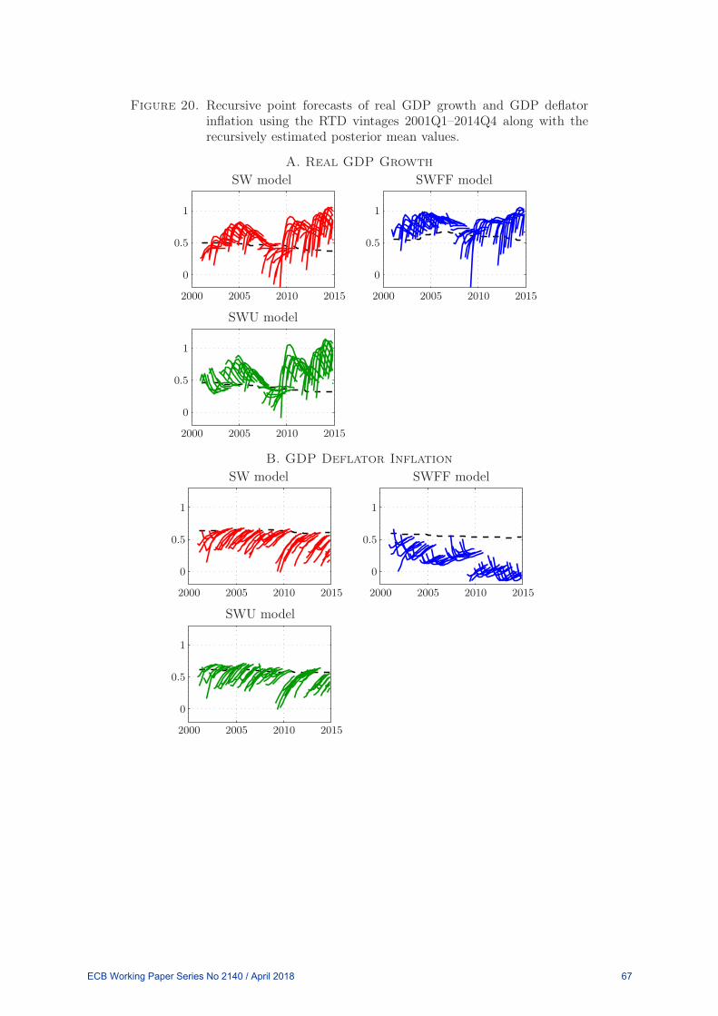
Figure 20. Recursive point forecasts of real GDP growth and GDP deflatorinflation using the RTD vintages 2001Q1–2014Q4 along with therecursively estimated posterior mean values.
A. Real GDP Growth
SW model SWFF model
SWU model
2000
20002000
2005
20052005
2010
20102010
2015
20152015
1
11
0.5
0.50.5
0
00
B. GDP Deflator Inflation
SW model SWFF model
SWU model
2000
20002000
2005
20052005
2010
20102010
2015
20152015
1
11
0.5
0.50.5
0
00
ECB Working Paper Series No 2140 / April 2018 67

Figure 21. Quarterly euro area data on the observable variables of the SW andSWU models for two vintages and their revisions.
A. Real-time Data 2008Q4 and 2009Q1
Real GDP, ∆yt Private consumption, ∆ct Total investment, ∆it
GDP deflator, πt Total employment, ∆et Real wages, ∆wt
Nominal interest rate, rt Unemployment, ut
2008Q4 vintage2009Q1 vintage
19801980
198019801980
198019801980
19901990
199019901990
199019901990
20002000
200020002000
200020002000
20102010
201020102010
201020102010
15 10
10 8
65
4
3
2
2
1
1
11
0.50.5
0
00
0
000
-0.5
-0.5 -1
-1-1 -2
B. Revisions in 2009Q1
Real GDP, ∆yt Private consumption, ∆ct Total investment, ∆it
GDP deflator, πt Total employment, ∆et Real wages, ∆wt
Nominal interest rate, rt Unemployment, ut
19951995
199519951995
199519951995
20002000
200020002000
200020002000
20052005
200520052005
200520052005
20102010
201020102010
201020102010
0.2
0.20.2
0.15
0.1
0.1
0.05
0.05
0.05
0.04
0.02
0.02
0
0
00
0
000
-0.02
-0.02-0.04
-0.05
-0.05
-0.06
-0.1
-0.1
-0.2
-0.2
-0.3-0.4
ECB Working Paper Series No 2140 / April 2018 68

Figure 22. Log predictive score for real GDP growth and inflation based onbackcasts, nowcasts, and one-to eight-quarter-head forecasts overthe vintages 2001Q1–2014Q4.
A. Monte Carlo integration
GDP deflator inflationReal GDP growth
Joint
20
10
8
8 8
6
6 6
4
4 4
2
2 2
0
0
0
0
0
0
-10
-20
-20
-40
-50
-60
-80
-100
SW modelSWFF modelSWU model
B. Normal approximation
GDP deflator inflationReal GDP growth
Joint
20
10
8
8 8
6
6 6
4
4 4
2
2 2
0
0
0
0
0
0
-10
-20
-20
-40
-50
-60
-80
-100
SW modelSWFF modelSWU model
Notes: Forecast horizons are displayed on the horizontal axis with h = −1 being the backcast horizon and h = 0
the nowcast horizon.
ECB Working Paper Series No 2140 / April 2018 69

Figure 23. Recursive estimates of the average log predictive score of realGDP growth and inflation using the MC estimator for the vintages2001Q1–2014Q4.
A. Real GDP growth
backcast nowcast one-q-ahead two-q-ahead
three-q-ahead four-q-ahead five-q-ahead six-q-ahead
seven-q-ahead eight-q-aheadSW modelSWFF modelSWU model
20002000
2000200020002000
2000200020002000
20052005
2005200520052005
2005200520052005
20102010
2010201020102010
2010201020102010
20152015
2015201520152015
2015201520152015
-0.5-0.5
-0.5-0.5-0.5-0.5
-0.5-0.5-0.5-0.5
-0.6
-0.7
-0.8
-0.9
-1-1
-1-1-1-1
-1-1-1
-1.5-1.5
-1.5-1.5-1.5-1.5
-1.5-1.5-1.5
B. GDP Deflator Inflation
backcast nowcast one-q-ahead two-q-ahead
three-q-ahead four-q-ahead five-q-ahead six-q-ahead
seven-q-ahead eight-q-aheadSW modelSWFF modelSWU model
20002000
2000200020002000
2000200020002000
20052005
2005200520052005
2005200520052005
20102010
2010201020102010
2010201020102010
20152015
2015201520152015
2015201520152015
1 0.5
0.40.4
0.40.40.40.4
0.40.4
0.20.2
0.20.20.20.2
0.20.2
00
0000
00
00
-0.2-0.2
-0.2-0.2-0.2-0.2
-0.2-0.2
-0.4-0.4
-0.4-0.4-0.4-0.4
-0.4-0.4
-0.5
-1-1
-1.5
-2-2
ECB Working Paper Series No 2140 / April 2018 70

Figure 23. Recursive estimates of the average log predictive score of realGDP growth and inflation using the MC estimator for the vintages2001Q1–2014Q4 (continued).
C. Real GDP growth & Inflation
backcast nowcast one-q-ahead two-q-ahead
three-q-ahead four-q-ahead five-q-ahead six-q-ahead
seven-q-ahead eight-q-aheadSW modelSWFF modelSWU model
20002000
2000200020002000
2000200020002000
20052005
2005200520052005
2005200520052005
20102010
2010201020102010
2010201020102010
20152015
2015201520152015
2015201520152015
00
0000
000
-0.5-0.5
-0.5-0.5-0.5-0.5
-0.5-0.5
-0.5
-1-1
-1-1-1-1
-1-1
-1-1
-1.5-1.5
-1.5-1.5-1.5-1.5
-1.5-1.5
-1.5
-2-2
-2-2-2-2
-2-2
-2
-2
-2.5
-3
-4
Figure 24. Recursive estimates of the average log predictive score of realGDP growth and inflation using the MC estimator for the vintages2008Q4–2014Q4.
A. Real GDP growthnowcast one-q-ahead two-q-ahead
three-q-ahead four-q-ahead five-q-ahead six-q-ahead
seven-q-ahead eight-q-aheadSW modelSWFF modelSWU model
20082008
2008200820082008
200820082008
20102010
2010201020102010
201020102010
20122012
2012201220122012
201220122012
20142014
2014201420142014
201420142014
00
-0.6-0.6
-0.6-0.6-0.6-0.6
-0.6
-0.8-0.8
-0.8-0.8-0.8-0.8
-0.8
-1-1
-1-1-1-1
-1
-1.2-1.2
-1.2-1.2-1.2-1.2
-1.2
-2-2
-4-4
-6
-6 -8
-8 -10
ECB Working Paper Series No 2140 / April 2018 71

Figure 24. Recursive estimates of the average log predictive score of realGDP growth and inflation using the MC estimator for the vintages2008Q4–2014Q4 (continued).
B. GDP Deflator Inflationbackcast nowcast one-q-ahead two-q-ahead
three-q-ahead four-q-ahead five-q-ahead six-q-ahead
seven-q-ahead eight-q-aheadSW modelSWFF modelSWU model
20082008
2008200820082008
2008200820082008
20102010
2010201020102010
2010201020102010
20122012
2012201220122012
2012201220122012
20142014
2014201420142014
2014201420142014
0.4
0.40.2
0.2
00
0000
00
0
0 -0.2
-0.5-0.5
-0.5-0.5-0.5-0.5
-0.5-0.5
-1-1
-1-1-1-1
-1-1
C. Real GDP growth & Inflationnowcast one-q-ahead two-q-ahead
three-q-ahead four-q-ahead five-q-ahead six-q-ahead
seven-q-ahead eight-q-aheadSW modelSWFF modelSWU model
20082008
2008200820082008
200820082008
20102010
2010201020102010
201020102010
20122012
2012201220122012
201220122012
20142014
2014201420142014
201420142014
00
-0.5-0.5
-0.5-0.5-0.5-0.5
-0.5
-1-1
-1-1-1-1
-1
-1.5-1.5
-1.5-1.5-1.5-1.5
-1.5
-2-2
-2-2-2-2
-2
-2-2
-4-4
-6
-6 -8
-8 -10
ECB Working Paper Series No 2140 / April 2018 72

Figure 25. Differences between the MC estimator and the normal approxima-tion of the recursive estimates in average log score of real GDPgrowth and inflation for the vintages 2001Q1–2014Q4.
A. Real GDP growth
backcast nowcast one-q-ahead two-q-ahead
three-q-ahead four-q-ahead five-q-ahead six-q-ahead
seven-q-ahead eight-q-aheadSW modelSWFF modelSWU model
20002000
2000200020002000
2000200020002000
20052005
2005200520052005
2005200520052005
20102010
2010201020102010
2010201020102010
20152015
2015201520152015
2015201520152015
0.050.05
0.050.050.050.05
0.050.050.050.05
00
0000
0000
-0.05-0.05
-0.05-0.05-0.05-0.05
-0.05-0.05-0.05-0.05
B. GDP Deflator Inflation
backcast nowcast one-q-ahead two-q-ahead
three-q-ahead four-q-ahead five-q-ahead six-q-ahead
seven-q-ahead eight-q-aheadSW modelSWFF modelSWU model
20002000
2000200020002000
2000200020002000
20052005
2005200520052005
2005200520052005
20102010
2010201020102010
2010201020102010
20152015
2015201520152015
2015201520152015
0.050.05
0.050.050.050.05
0.050.050.050.05
00
0000
0000
-0.05-0.05
-0.05-0.05-0.05-0.05
-0.05-0.05-0.05-0.05
ECB Working Paper Series No 2140 / April 2018 73

Figure 25. Differences between the MC estimator and the normal approxima-tion of the recursive estimates in average log score of real GDPgrowth and inflation for the vintages 2001Q1–2014Q4 (continued).
C. Real GDP growth & Inflation
backcast nowcast one-q-ahead two-q-ahead
three-q-ahead four-q-ahead five-q-ahead six-q-ahead
seven-q-ahead eight-q-aheadSW modelSWFF modelSWU model
20002000
2000200020002000
2000200020002000
20052005
2005200520052005
2005200520052005
20102010
2010201020102010
2010201020102010
20152015
2015201520152015
2015201520152015
0.050.05
0.050.050.050.05
0.050.050.050.05
00
0000
0000
-0.05-0.05
-0.05-0.05-0.05-0.05
-0.05-0.05-0.05-0.05
ECB Working Paper Series No 2140 / April 2018 74

Figure 26. Recursive estimates of the share of parameter uncertainty of thepredictive variances of real GDP growth and inflation for the vin-tages 2001Q1–2014Q4.
A. Real GDP growth
backcast nowcast one-q-ahead two-q-ahead
three-q-ahead four-q-ahead five-q-ahead six-q-ahead
seven-q-ahead eight-q-aheadSW modelSWFF modelSWU model
20002000
2000200020002000
2000200020002000
20052005
2005200520052005
2005200520052005
20102010
2010201020102010
2010201020102010
20152015
2015201520152015
2015201520152015
0.10.1
0.10.10.10.1
0.10.10.10.1
0.080.08
0.080.080.080.08
0.080.080.080.08
0.060.06
0.060.060.060.06
0.060.060.060.06
0.040.04
0.040.040.040.04
0.040.040.040.04
0.020.02
0.020.020.020.02
0.020.020.020.02
00
0000
0000
B. GDP Deflator Inflation
backcast nowcast one-q-ahead two-q-ahead
three-q-ahead four-q-ahead five-q-ahead six-q-ahead
seven-q-ahead eight-q-aheadSW modelSWFF modelSWU model
20002000
2000200020002000
2000200020002000
20052005
2005200520052005
2005200520052005
20102010
2010201020102010
2010201020102010
20152015
2015201520152015
2015201520152015
0.10.1
0.10.10.10.1
0.10.10.10.1
0.080.08
0.080.080.080.08
0.080.080.080.08
0.060.06
0.060.060.060.06
0.060.060.060.06
0.040.04
0.040.040.040.04
0.040.040.040.04
0.020.02
0.020.020.020.02
0.020.020.020.02
00
0000
0000
ECB Working Paper Series No 2140 / April 2018 75

Figure 27. Decomposition of recursive estimates of the average log predictivescore of real GDP growth using the normal approximation for thevintages 2001Q1–2014Q4.
A. Forecast uncertainty
backcast nowcast one-q-ahead two-q-ahead
three-q-ahead four-q-ahead five-q-ahead six-q-ahead
seven-q-ahead eight-q-aheadSW modelSWFF modelSWU model
20002000
2000200020002000
2000200020002000
20052005
2005200520052005
2005200520052005
20102010
2010201020102010
2010201020102010
20152015
2015201520152015
2015201520152015
0.6
0.40.4
0.40.40.40.4
0.40.40.4
0.4
0.20.2
0.20.20.20.2
0.20.20.2
0.2
00
0000
000
0
-0.2-0.2
-0.2-0.2-0.2-0.2
-0.2-0.2-0.2
-0.2
-0.4-0.4
-0.4-0.4-0.4-0.4
-0.4-0.4-0.4
B. Quadratic standardized forecast error
backcast nowcast one-q-ahead two-q-ahead
three-q-ahead four-q-ahead five-q-ahead six-q-ahead
seven-q-ahead eight-q-aheadSW modelSWFF modelSWU model
20002000
2000200020002000
2000200020002000
20052005
2005200520052005
2005200520052005
20102010
2010201020102010
2010201020102010
20152015
2015201520152015
2015201520152015
00
0000
0000
-0.2-0.2
-0.2-0.2-0.2-0.2
-0.2-0.2-0.2-0.2
-0.4-0.4
-0.4-0.4-0.4-0.4
-0.4-0.4-0.4-0.4
-0.6-0.6
-0.6-0.6-0.6-0.6
-0.6-0.6-0.6-0.6
-0.8-0.8
-0.8-0.8-0.8-0.8
-0.8-0.8-0.8-0.8
ECB Working Paper Series No 2140 / April 2018 76

Figure 28. Decomposition of recursive estimates of the average log predictivescore of inflation using the normal approximation for the vintages2001Q1–2014Q4.
A. Forecast uncertainty
backcast nowcast one-q-ahead two-q-ahead
three-q-ahead four-q-ahead five-q-ahead six-q-ahead
seven-q-ahead eight-q-aheadSW modelSWFF modelSWU model
20002000
2000200020002000
2000200020002000
20052005
2005200520052005
2005200520052005
20102010
2010201020102010
2010201020102010
20152015
2015201520152015
2015201520152015
33
2.52.5
22
1.51.5
1.41.4
1.41.41.41.4
1.41.4
1.21.2
1.21.21.21.2
1.21.2
11
1111
11
11
0.80.8
0.80.80.80.8
0.80.8
0.60.6
0.60.60.60.6
0.60.6
B. Quadratic standardized forecast error
backcast nowcast one-q-ahead two-q-ahead
three-q-ahead four-q-ahead five-q-ahead six-q-ahead
seven-q-ahead eight-q-aheadSW modelSWFF modelSWU model
20002000
2000200020002000
2000200020002000
20052005
2005200520052005
2005200520052005
20102010
2010201020102010
2010201020102010
20152015
2015201520152015
2015201520152015
00
0000
0000
-0.2-0.2
-0.2-0.2-0.2-0.2
-0.2-0.2
-0.4-0.4
-0.4-0.4-0.4-0.4
-0.4-0.4
-0.5-0.5
-0.6-0.6
-0.6-0.6-0.6-0.6
-0.6-0.6
-1-1
-1.5-1.5
-2-2
ECB Working Paper Series No 2140 / April 2018 77

Figure 29. Decomposition of recursive estimates of the average log predictivescore of inflation and real GDP growth using the normal approxi-mation for the vintages 2001Q1–2014Q4.
A. Forecast uncertainty
backcast nowcast one-q-ahead two-q-ahead
three-q-ahead four-q-ahead five-q-ahead six-q-ahead
seven-q-ahead eight-q-aheadSW modelSWFF modelSWU model
20002000
2000200020002000
2000200020002000
20052005
2005200520052005
2005200520052005
20102010
2010201020102010
2010201020102010
20152015
2015201520152015
2015201520152015
4
3
2.5
22
2222
22
2
2
1.51.5
1.51.51.51.5
1.51.51.5
11
1111
111
1
0.50.5
0.50.50.50.5
0.50.5
0.5
00
B. Quadratic standardized forecast error
backcast nowcast one-q-ahead two-q-ahead
three-q-ahead four-q-ahead five-q-ahead six-q-ahead
seven-q-ahead eight-q-aheadSW modelSWFF modelSWU model
20002000
2000200020002000
2000200020002000
20052005
2005200520052005
2005200520052005
20102010
2010201020102010
2010201020102010
20152015
2015201520152015
2015201520152015
00
0000
0000
-0.5-0.5
-0.5-0.5-0.5-0.5
-0.5-0.5-0.5
-1-1
-1-1-1-1
-1-1
-1
-1
-1.5-1.5
-1.5-1.5-1.5-1.5
-1.5-1.5
-1.5
-2
-2
-2.5
-3
-4
ECB Working Paper Series No 2140 / April 2018 78

References
Adolfson, M., Laséen, S., Lindé, J., and Villani, M. (2005), “Are Constant Interest Rate Forecasts
Modest Policy Interventions? Evidence from a Dynamic Open-Economy Model,” International
Finance, 8(3), 509–544.
Adolfson, M., Laséen, S., Lindé, J., and Villani, M. (2007a), “Bayesian Estimation of an Open
Economy DSGE Model with Incomplete Pass-Through,” Journal of International Economics,
72(2), 481–511.
Adolfson, M., Lindé, J., and Villani, M. (2007b), “Forecasting Performance of an Open Economy
DSGE Model,” Econometric Reviews, 26(2), 289–328.
Amisano, G. and Geweke, J. (2017), “Prediction Using Several Macroeconomic Models,” Review
of Economics and Statistics, 99(5), 912–925.
An, S. and Schorfheide, F. (2007), “Bayesian Analysis of DSGE Models,” Econometric Reviews,
26(2), 113–172.
Bernanke, B. S., Gertler, M., and Gilchrist, S. (1999), “The Financial Accelerator in a Quanti-
tative Business Cycle Framework,” in J. B. Taylor and M. Woodford (Editors), Handbook of
Macroeconomics, volume 1C, 1341–1393, North Holland, Amsterdam.
Buch, C. M. and Holtemöller, O. (2014), “Do we need New Modelling Approaches in Macroe-
conomics?” in Financial Cycles and the Real Economy, chapter 3, 36–58, Edward Elgar
Publishing.
Caballero, R. J. (2010), “Macroeconomics after the Crisis: Time to Deal with the Pretense-of-
Knowledge Syndrome,” Journal of Economic Perspectives, 24(4), 85–102.
Canova, F. and Sala, L. (2009), “Back to Square One: Identification Issues in DSGE Models,”
Journal of Monetary Economics, 56(4), 431–449.
Cantore, C., León-Ledesma, M., McAdam, P., and Willman, A. (2014), “Shocking Stuff: Tech-
nology, Hours, And Factor Substitution,” Journal of the European Economic Association,
12(1), 108–128.
Carlstrom, C. T., Fuerst, T. S., and Paustian, M. (2017), “Targeting Long Rates in a Model
with Segmented Markets,” American Economic Journal: Macroeconomics, 9(1), 205–242.
Chari, V. V., Kehoe, P. J., and McGrattan, E. R. (2009), “New Keynesian Models: Not Yet
Useful for policy Analysis,” American Economic Journal: Macroeconomics, 1(1), 242–266.
Chetty, R., Guren, A., Manoli, D., and Weber, A. (2011), “Are Micro and Macro Labor Supply
Elasticities Consistent? A Review of Evidence on the Intensive and Extensive Margins,”
American Economic Review, 101(3), 471–475.
Christiano, L. J., Motto, R., and Rostagno, M. (2003), “The Great Depression and the Friedman-
Schwartz Hypothesis,” Journal of Money, Credit, and Banking, 35(6), 1119–1197.
Christiano, L. J., Motto, R., and Rostagno, M. (2008), “Shocks, Structures or Monetary Policies?
The Euro Area and US After 2001,” Journal of Economic Dynamics and Control, 32(8), 2476–
2506.
ECB Working Paper Series No 2140 / April 2018 79

Christiano, L. J., Motto, R., and Rostagno, M. (2010), “Financial Factors in Economic Fluctu-
ations,” ECB Working Paper Series No. 1192.
Christiano, L. J., Trabandt, M., and Walentin, K. (2011), “Introducing Financial Frictions and
Unemployment into a Small Open Economy Model,” Journal of Economic Dynamics and
Control, 35(12), 1999–2041.
Coenen, G., Karadi, P., Schmidt, S., and Warne, A. (2018), “The New Area-Wide Model II:
An Updated Version of the ECB’s Micro-Founded Model for Forecasting and Policy Analysis
with a Financial Sector,” Unpublished Manuscript.
Coenen, G., Levin, A., and Wieland, V. (2005), “Data Uncertainty and the Role of Money as
Information Variable for Monetary Policy,” European Economic Review, 49(4), 975–1006.
Coenen, G. and Warne, A. (2014), “Risks to Price Stability, the Zero Lower Bound and Forward
Guidance: A Real-Time Assessment,” International Journal of Central Banking, 10(2), 7–54.
Conflitti, C., De Mol, C., and Giannone, D. (2015), “Optimal Combination of Survey Forecasts,”
International Journal of Forecasting, 31(4), 1096–1103.
Consolo, A., Favero, C. A., and Paccagnini, A. (2009), “On the Statistical Identification of DSGE
Models,” Journal of Econometrics, 150(1), 99–115.
Croushore, D. (2011), “Frontiers of Real-Time Data Analysis,” Journal of Economic Literature,
49(1), 72–110.
Croushore, D. and Stark, T. (2001), “A Real-Time Data Set for Macroeconomists,” Journal of
Econometrics, 105(1), 111–130.
Darracq Paries, M., Kok Sørensen, C., and Rodriguez-Palenzuela, D. (2011), “Macroeconomic
Propagation under Different Regulatory Regimes: Evidence from an Estimated DSGE Model
for the Euro Area,” International Journal of Central Banking, 7(4), 49–113.
De Graeve, F. (2008), “The External Finance Premium and the Macroeconomy: US Post-WWII
Evidence,” Journal of Economic Dynamics and Control, 32(11), 3415–3440.
Del Negro, M., Eusepi, S., Giannoni, M., Sbordone, A., Tambalotti, A., Cocci, M., Hasegawa,
R., and Linder, M. H. (2013), “The FRBNY DSGE Model,” Federal Reserve Bank of New
York Staff Reports No. 647.
Del Negro, M., Giannoni, M. P., and Schorfheide, F. (2015), “Inflation in the Great Recession
and New Keynesian Models,” American Economic Journal: Macroeconomics, 7(1), 168–196.
Del Negro, M. and Schorfheide, F. (2013), “DSGE Model-Based Forecasting,” in G. Elliott
and A. Timmermann (Editors), Handbook of Economic Forecasting, volume 2, 57–140, North
Holland, Amsterdam.
Durbin, J. and Koopman, S. J. (2012), Time Series Analysis by State Space Methods, Oxford
University Press, Oxford, 2nd edition.
European Commission (2016), “Labour Market and Wage Developments in Europe Annual Re-
view,” European Commission.
ECB Working Paper Series No 2140 / April 2018 80

Fagan, G., Henry, J., and Mestre, R. (2005), “An Area-Wide Model for the Euro Area,” Economic
Modelling, 22(1), 39–59.
Fisher, J. D. M. (2015), “On the Structural Interpretation of the Smets-Wouters “Risk Premium”
Shock,” Journal of Money, Credit and Banking, 47(2–3), 511–516.
Galí, J. (2011), “The Return Of The Wage Phillips Curve,” Journal of the European Economic
Association, 9(3), 436–461.
Galí, J., Smets, F., and Wouters, R. (2012), “Unemployment in an Estimated New Keynesian
Model,” in D. Acemoglu and M. Woodford (Editors), NBER Macroeconomics Annual 2011,
329–360, University of Chicago Press.
Gelman, A., Carlin, J. B., Stern, H. S., and Rubin, D. B. (2004), Bayesian Data Analysis,
Chapman & Hall/CRC, Boca Raton, 2nd edition.
Gerali, A., Neri, S., Sessa, L., and Signoretti, F. M. (2010), “Credit and Banking in a DSGE
Model of the Euro Area,” Journal of Money, Credit and Banking, 42(s1), 107–141.
Gertler, M. and Karadi, P. (2011), “A Model of Unconventional Monetary Policy,” Journal of
Monetary Economics, 58(1), 17–34.
Gertler, M. and Karadi, P. (2013), “Qe 1 vs. 2 vs. 3 . . . : A framework for analyzing large-scale
asset purchases as a monetary policy tool,” International Journal of Central Banking, 9(1),
5–53.
Geweke, J. and Amisano, G. (2011), “Optimal Prediction Pools,” Journal of Econometrics,
164(1), 130–141.
Geweke, J. and Amisano, G. (2014), “Analysis of Variance for Bayesian Inference,” Econometric
Reviews, 33(1–4), 270–288.
Giannone, D., Henry, J., Lalik, M., and Modugno, M. (2012), “An Area-Wide Real-Time Data-
base for the Euro Area,” Review of Economics and Statistics, 94(4), 1000–1013.
Gneiting, T. and Raftery, A. E. (2007), “Strictly Proper Scoring Rules, Prediction, and Estima-
tion,” Journal of the American Statistical Association, 102(477), 359–378.
Hall, R. E. (2010), “Why Does the Economy Fall to Pieces after a Financial Crisis?” Journal of
Economic Perspectives, 24(4), 45–66.
Harvey, A. C. (1989), Forecasting, Structural Time Series Models and the Kalman Filter, Cam-
bridge University Press, Cambridge.
Herbst, E. P. (2015), “Using the “Chandrasekhar Recursions” for Likelihood Evaluation of DSGE
Models,” Computational Economics, 45(4), 693–705.
Iacoviello, M. (2005), “House Prices, Borrowing Constraints, and Monetary Policy in the Busi-
ness Cycle,” American Economic Review, 95(3), 739–764.
Iskrev, N. (2010), “Local Identification in DSGE Models,” Journal of Monetary Economic, 57(2),
189–202.
Jarociński, M. and Lenza, M. (2016), “An Inflation-Predicting Measure of the Output Gap in the
Euro Area,” Journal of Money, Credit and Banking, Forthcoming; available as ECB Working
ECB Working Paper Series No 2140 / April 2018 81

Paper Series No. 1966.
Kimball, M. S. (1995), “The Quantitative Analytics of the Basic Nonmonetarist Model,” Journal
of Money, Credit, and Banking, 27(4), 1241–77.
Kolasa, M. and Rubaszek, M. (2015), “Forecasting using DSGE Models with Financial Frictions,”
International Journal of Forecasting, 31(1), 1–19.
Kolasa, M., Rubaszek, M., and Skrzypczyński, P. (2012), “Putting the New Keynesian DSGE
Model to the Real-Time Forecasting Test,” Journal of Money, Credit, and Banking, 44(7),
1301–1324.
Komunjer, I. and Ng, S. (2011), “Dynamic Identification of Dynamic Stochastic General Equi-
librium Models,” Econometrica, 79(6), 1995–2032.
Krishnamurthy, A. and Vissing-Jorgensen, A. (2012), “The Aggregate Demand for Treasury
Debt,” Journal of Political Economy, 120(2), 233–267.
Levine, P., McAdam, P., and Pearlman, J. (2008), “Quantifying and Sustaining Welfare Gains
from Monetary Commitment,” Journal of Monetary Economics, 55(7), 1253–1276.
Lindé, J., Smets, F., and Wouters, R. (2016), “Challenges for Central Banks’ Macro Models,”
in J. B. Taylor and H. Uhlig (Editors), Handbook of Macroeconomics, volume 2B, 2185–2262,
North Holland, Amsterdam.
Lombardo, G. and McAdam, P. (2012), “Financial Market Frictions in a Model of the Euro
Area,” Economic Modelling, 29(6), 2460–2485.
Ohanian, L. (2010), “The Economic Crisis from a Neoclassical Perspective,” Journal of Economic
Perspectives, 24(4), 45–66.
Peterman, W. B. (2016), “Reconciling Micro And Macro Estimates Of The Frisch Labor Supply
Elasticity,” Economic Inquiry, 54(1), 100–120.
Pirschel, I. (2016), “Forecasting Euro Area Recessions in Real-Time,” Kiel Working Paper, No.
2020.
Smets, F., Warne, A., and Wouters, R. (2014), “Professional Forecasters and Real-Time Fore-
casting with a DSGE Model,” International Journal of Forecasting, 30(4), 981–995.
Smets, F. and Wouters, R. (2003), “An Estimated Stochastic Dynamic General Equilibrium
Model for the Euro Area,” Journal of the European Economic Association, 1(5), 1123–1175.
Smets, F. and Wouters, R. (2005), “Comparing Shocks and Frictions in U.S. and Euro Area
Business Cycles: A Bayesian DSGE Approach,” Journal of Applied Econometrics, 20(2), 161–
183.
Smets, F. and Wouters, R. (2007), “Shocks and Frictions in US Business Cycles: A Bayesian
DSGE Approach,” American Economic Review, 97(3), 586–606.
Tierney, L. (1994), “Markov Chains for Exploring Posterior Distributions,” The Annals of Sta-
tistics, 22(4), 1701–1728, with discussion, p. 1728–1762.
Wallis, K. F. (1986), “Forecasting with an Econometric Model: The Ragged Edge Problem,”
Journal of Forecasting, 5(1), 1–13.
ECB Working Paper Series No 2140 / April 2018 82

Warne, A. (2017), “YADA Manual — Computational Details,” Manuscript, European Central
Bank. Available with the YADA distribution.
Warne, A., Coenen, G., and Christoffel, K. (2017), “Marginalized Predictive Likelihood Com-
parisons of Linear Gaussian State-Space Models with Applications to DSGE, DSGE-VAR and
VAR Models,” Journal of Applied Econometrics, 32(1), 103–119.
ECB Working Paper Series No 2140 / April 2018 83

Appendix: A Detailed Exposition of the DSGE Models
A.1. The Smets and Wouters Model Adapted to the Euro Area
A well known example of a medium-sized DSGE model is Smets and Wouters (2007), where
the authors study shocks and frictions in US business cycles. The equations of the model are
presented below, while a detailed discussion of the model is found in Smets and Wouters (2007);
see also Smets and Wouters (2003, 2005). It should be emphasized that since the model uses
a flexible-price based output gap measure in the monetary policy rule, the discussion will first
consider the sticky price and wage system, followed by the flexible price and wage system. The
equations for the seven exogenous variables are introduced thereafter, while the steady-state of
the system closes the theoretical part of the empirical model. Finally, the model variables are
linked to the observed variables via the measurement equations.
A.2. The Sticky Price and Wage Equations
The log-linearized aggregate resource constraint of this closed economy model is given by
yt = cy ct + iy it + zyzt + εgt , (A.1)
where yt is (detrended) real GDP. It is absorbed by real private consumption (ct), real private
investments (it), the capital utilization rate (zt), and exogenous spending (εgt ). The parameter
cy is the steady-state consumption-output ratio and iy is the steady-state investment-output
ratio, where
cy = 1 − iy − gy,
and gy is the steady-state exogenous spending-output ratio. The steady-state investment-output
ratio is determined by
iy = (γ + δ − 1) ky,
where ky is the steady-state capital-output ratio, γ is the steady-state growth rate, and δ is the
depreciation rate of capital. Finally,
zy = rkky,
where rk is the steady-state rental rate of capital. The steady-state parameters are shown in
Section A.5, but it is noteworthy already at this stage that zy = α, the share of capital in
production.
The dynamics of consumption follows from the consumption Euler equation and is equal to
ct = c1ct−1 + (1 − c1)Etct+1 + c2
(lt − Et lt+1
)− c3
(rt − Etπt+1
)+ εbt , (A.2)
where lt is hours worked, rt is the policy controlled nominal interest rate, and εbt is proportional
to the exogenous risk premium, i.e., a wedge between the interest rate controlled by the central
bank and the return on assets held by households. It should be noted that in contrast to Smets
and Wouters (2007), but identical to Smets and Wouters (2005) and Lindé et al. (2016), we have
ECB Working Paper Series No 2140 / April 2018 84

moved the risk premium variable outside the expression for the ex ante real interest rate. This
means that εbt = −c3εbt , where εbt is the risk premium variable in Smets and Wouters (2007).
Building on the work by Krishnamurthy and Vissing-Jorgensen (2012), Fisher (2015) shows that
this shock can be given a structural interpretation, namely, as a shock to the demand for safe
and liquid assets or, alternatively, as a liquidity preference shock.
The parameters of the consumption Euler equation are:
c1 =λ/γ
1 + (λ/γ), c2 =
(σc − 1) (whl/c)σc (1 + (λ/γ))
, c3 =1 − (λ/γ)
σc (1 + (λ/γ)),
where λ measures external habit formation, σc is the inverse of the elasticity of intertemporal
substitution for constant labor, while whl/c is the steady-state hourly real wage bill to consump-
tion ratio. If σc = 1 (log-utility) and λ = 0 (no external habit) then the above equation reduces
to the familiar purely forward looking consumption Euler equation.
The log-linearized investment Euler equation is given by
it = i1 it−1 + (1 − i1)Etit+1 + i2qt + εit, (A.3)
where qt is the real value of the existing capital stock, while εit is an exogenous investment-specific
technology variable. The parameters of (A.3) are given by
i1 =1
1 + βγ1−σc, i2 =
1(1 + βγ1−σc) γ2ϕ
,
where β is the discount factor used by households, and ϕ is the steady-state elasticity of the
capital adjustment cost function.
The dynamic equation for the value of the capital stock is
qt = q1Etqt+1 + (1 − q1)Etrkt+1 −(rt − Etπt+1
)+ c−1
3 εbt , (A.4)
where rkt is the rental rate of capital. The parameter q1 is here given by
q1 = βγ−σc(1 − δ) =1 − δ
rk + 1 − δ.
Turning to the supply-side of the economy, the log-linearized aggregate production function
can be expressed as
yt = φp
[αkst + (1 − α) lt + εat
], (A.5)
where kst is capital services used in production, and εat an exogenous total factor productivity
variable. As mentioned above, the parameter α reflects the share of capital in production, while
φp is equal to one plus the steady-state share of fixed costs in production.
The capital services variable is used to reflect that newly installed capital only becomes
effective with a one period lag. This means that
kst = kt−1 + zt, (A.6)
ECB Working Paper Series No 2140 / April 2018 85

where kt is the installed capital. The degree of capital utilization is determined from cost
minimization of the households that provide capital services and is therefore a positive function
of the rental rate of capital. Specifically,
zt = z1rkt , (A.7)
where
z1 =1 − ψ
ψ,
and ψ is a positive function of the elasticity of the capital adjustment cost function and nor-
malized to lie between 0 and 1. The larger ψ is the costlier it is to change the utilization of
capital.
The log-linearized equation that specifies the development of installed capital is
kt = k1kt−1 + (1 − k1) it + k2εit. (A.8)
The two parameters are given by
k1 =1 − δ
γ, k2 = (γ + δ − 1)
(1 + βγ1−σc
)γϕ.
From the monopolistically competitive goods market, the price markup (µpt ) is equal to minus
the real marginal cost (µct) under cost minimization by firms. That is,
µpt = α(kst − lt
)− wt + εat , (A.9)
where the real wage is given by wt. Similarly, the real marginal cost is
µct = αrkt + (1 − α) wt − εat , (A.10)
where (A.10) is obtained by substituting for the optimally determined capital-labor ratio in
equation (A.12).
Due to price stickiness, and partial indexation to lagged inflation of those prices that cannot
be re-optimized, prices adjust only sluggishly to their desired markups. Profit maximization by
price-setting firms yields the log-linearized price Phillips curve
πt = π1πt−1 + π2Etπt+1 − π3µpt + εpt
= π1πt−1 + π2Etπt+1 + π3µct + εpt ,
(A.11)
where εpt is an exogenous price markup process. The parameters of the Phillips curve are given
by
π1 =ıp
1 + βγ1−σc ıp, π2 =
βγ1−σc
1 + βγ1−σc ıp, π3 =
(1 − ξp)(1 − βγ1−σcξp
)(1 + βγ1−σc ıp) ξp ((φp − 1)εp + 1)
.
The degree of indexation to past inflation is determined by the parameter ıp, ξp measures the
degree of price stickiness such that 1− ξp is the probability that a firm can re-optimize its price,
and εp is the curvature of the Kimball (1995) goods market aggregator.
ECB Working Paper Series No 2140 / April 2018 86

Cost minimization of firms also implies that the rental rate of capital is related to the capital-
labor ratio and the real wage according to.
rkt = −(kst − lt
)+ wt. (A.12)
In the monopolistically competitive labor market the wage markup is equal to the difference
between the real wage and the marginal rate of substitution between labor and consumption
µwt = wt −(σl lt +
11 − (λ/γ)
[ct − λ
γct−1
]), (A.13)
where σl is the elasticity of the labor input with respect to real wages.
Due to wage stickiness and partial wage indexation, real wages respond gradually to the
desired wage markup
wt = w1wt−1 + (1 −w1)[Etwt+1 + Etπt+1
]−w2πt + w3πt−1 − w4µwt + εwt , (A.14)
where εwt is an exogenous wage markup process. The parameters of the wage equation are
w1 =1
1 + βγ1−σc, w2 =
1 + βγ1−σc ıw1 + βγ1−σc
,
w3 =ıw
1 + βγ1−σc, w4 =
(1 − ξw)(1 − βγ1−σcξw
)(1 + βγ1−σc) ξw ((φw − 1) εw + 1)
.
The degree of wage indexation to past inflation is given by the parameter ıw, while ξw is the
degree of wage stickiness. The steady-state labor market markup is equal to φw − 1 and εw is
the curvature of the Kimball labor market aggregator.
The sticky price and wage part of the model is closed by adding the monetary policy reaction
function
rt = ρrt−1 + (1 − ρ)[rππt + ry
(yt − yft
)]+ r∆y
[∆yt − ∆yft
]+ εrt , (A.15)
where yft is potential output measured as the level of output that would prevail under flexible
prices and wages in the absence of the two exogenous markup processes, whereas εrt is an
exogenous monetary policy shock process.
As productivity is written in terms of hours worked, we introduce an auxiliary equation with
Calvo-rigidity to link from observed total employment (et) to unobserved hours worked:
et − et−1 = β(Etet+1 − et
)+
(1 − βξe
)(1 − ξe
)ξe
(lt − et
), (A.16)
where 1− ξe is the fraction of firms that are able to adjust employment to its desired total labor
input; see Adolfson et al. (2005, 2007a).
A.3. The Flexible Price and Wage Equations
The flexible price equations are obtained by assuming that the two exogenous markup processes
are zero, while ξw = ξp = 0, and ıw = ıp = 0. As a consequence, inflation is always equal to
the steady-state inflation rate while real wages are equal to the marginal rate of substitution
ECB Working Paper Series No 2140 / April 2018 87

between labor and consumption as well as to the marginal product of labor. All other aspects
of the economy are unaffected. Letting the superscript f denote the flexible price and wage
economy versions of the variables we find that
yft = cy cft + iy i
ft + zy z
ft + εgt ,
cft = c1cft−1 + (1 − c1)Etc
ft+1 + c2
(lft − Et l
ft+1
)− c3r
ft + εbt ,
ift = i1 ift−1 + (1 − i1)Eti
ft+1 + i2q
ft + εit,
qft = q1Etqft+1 + (1 − q1)Etr
k,ft+1 − rft + c−1
3 εbt ,
yft = φp
[αks,ft + (1 − α) lft + εat
],
ks,ft = kft−1 + zft ,
zft = z1rk,ft ,
kft = k1kft−1 + (1 − k1) i
ft + k2ε
it,
εat = αrk,ft + (1 − α) wft ,
rk,ft = −(ks,ft − lft
)+ wft ,
wft = σl lft +
11 − (λ/γ)
[cft −
λ
γcft−1
],
eft − eft−1 = β(Ete
ft+1 − eft
)+
(1 − βξe
)(1 − ξe
)ξe
(lft − eft
),
(A.17)
where rft is the real interest rate of the flexible price and wage system.
A.4. The Exogenous Variables
There are seven exogenous processes in the Smets and Wouters (2007) model. These are generally
modelled as AR(1) processes with the exception of the exogenous spending process (where the
process depends on both the exogenous spending shock ηgt and the total factor productivity
shock ηat ) and the exogenous price and wage markup processes, which are treated as ARMA(1, 1)
processes. This means that
εgt = ρgεgt−1 + σgη
gt + ρgaσaη
at ,
εbt = ρbεbt−1 + σbη
bt ,
εit = ρiεit−1 + σiη
it,
εat = ρaεat−1 + σaη
at ,
εpt = ρpεpt−1 + σpη
pt − µpσpη
pt−1,
εwt = ρwεwt−1 + σwη
wt − µwσwη
wt−1,
εrt = ρrεrt−1 + σrη
rt .
(A.18)
ECB Working Paper Series No 2140 / April 2018 88

The shocks ηjt , j = {a, b, g, i, p, r, w}, are N(0, 1), where ηbt is a preference shock (proportional
to a risk premium shock), ηit is an investment-specific technology shock, ηpt is a price markup
shock, ηrt is a monetary policy or interest rate shock, and ηwt is a wage markup shock.
A.5. The Steady-State Equations
It remains to provide expressions for the steady-state values of the capital-output ratio, the
rental rate of capital, and the hourly real wage bill to consumption ratio which relate them
to the parameters of the model. The steady-state exogenous spending to output ratio gy is a
calibrated parameter and set to 0.18 by Smets and Wouters (2007). From the expressions for
the q1 parameter it follows that
rk =1
βγ−σc+ δ − 1.
The capital-output ratio is derived in a stepwise manner in the model appendix to Smets and
Wouters (2007). The steady-state relations there are
w =
[αα (1 − α)(1−α)
φp (rk)α
]1/(1−α)
,l
k=
(1 − α) rk
αw,
k
y= φp
[l
k
]α−1
,
where ky = k/y. From these relationships it is straightforward, albeit tedious, to show that
zy = rkky = α.
The steady-state relation between real wages and hourly real wages is
w = φwwh,
so that the steady-state hourly real wage bill to consumption ratio is given by
whl
c=
(1 − α) rkkyφwαcy
=1 − α
φwcy,
where the last equality follows from the relationship of zy = rkky = α.
A.6. The Measurement Equations
The Smets and Wouters (2007) model is consistent with a balanced steady-state growth path
driven by deterministic labor augmenting technological progress. The observed variables for the
euro area are given by quarterly data of the log of real GDP for the euro area (yt), the log of real
private consumption (ct), the log of real total investment (it), the log of total employment (et),
the log of quarterly GDP deflator inflation (πt), the log of real wages (wt), and the short-term
nominal interest rate (rt) given by the 3-month EURIBOR rate. The measurement equations
ECB Working Paper Series No 2140 / April 2018 89

are given by ⎡⎢⎢⎢⎢⎢⎢⎢⎢⎢⎢⎢⎢⎢⎢⎢⎢⎢⎢⎣
∆yt
∆ct
∆it
∆wt
∆et
πt
rt
⎤⎥⎥⎥⎥⎥⎥⎥⎥⎥⎥⎥⎥⎥⎥⎥⎥⎥⎥⎦
=
⎡⎢⎢⎢⎢⎢⎢⎢⎢⎢⎢⎢⎢⎢⎢⎢⎢⎢⎢⎣
γ + e
γ + e
γ + e
γ
e
π
4r
⎤⎥⎥⎥⎥⎥⎥⎥⎥⎥⎥⎥⎥⎥⎥⎥⎥⎥⎥⎦
+
⎡⎢⎢⎢⎢⎢⎢⎢⎢⎢⎢⎢⎢⎢⎢⎢⎢⎢⎢⎣
yt − yt−1
ct − ct−1
it − it−1
wt − wt−1
et − et−1
πt
4rt
⎤⎥⎥⎥⎥⎥⎥⎥⎥⎥⎥⎥⎥⎥⎥⎥⎥⎥⎥⎦
. (A.19)
Since all observed variables except the short-term nominal interest rate (which is already reported
in percent) are multiplied by 100, it follows that the steady-state values on the right hand side
are given by
γ = 100 (γ − 1) , π = 100 (π − 1) , r = 100(
π
βγ−σc− 1),
where π is steady-state inflation while e reflects steady-state labor force growth. The interest
rate in the model, rt, is measured in quarterly terms in the model and is therefore multiplied by
4 in (A.19) to restore it to annual terms for the measurement.
Apart from the steady-state exogenous spending-output ratio only six additional parameters
are calibrated. These are δ = 0.025, φw = 1.5, εp = εw = 10, and µp = µw = 0. The latter two
parameters are estimated by Smets and Wouters (2007) on US data, but we have here opted to
treat all exogenous processes in the model symmetrically. The remaining 20 structural and 15
shock process parameters are estimated. When estimating the parameters, we make us of the
following transformation of the discount factor
β =1
1 +(β/100
) .Following Smets and Wouters (2007), a prior distribution is assumed for the parameter β, while
β is determined from the above equation.
A.7. The Smets and Wouters Model with Financial Frictions
Changes to the Sticky Economy
Lombardo and McAdam (2012), Del Negro and Schorfheide (2013) and Del Negro et al. (2015)
introduce financial frictions into variants of the Smets and Wouters model based on the financial
accelerator approach of Bernanke et al. (1999); see also Christiano et al. (2003); Christiano,
Motto, and Rostagno (2010) and De Graeve (2008). This amounts to replacing the value of the
capital stock equation in (A.4) with
Etret+1 − rt = ζsp,b
(qt + kt − nt
)− c−13 εbt + εet , (A.20)
ECB Working Paper Series No 2140 / April 2018 90

and
ret − πt =(1 − q1
)rkt + q1qt − qt−1, (A.21)
where ret is the gross return on capital for entrepreneurs, nt is entrepreneurial equity (net worth),
and εet captures mean-preserving changes in the cross-sectional dispersion of ability across en-
trepreneurs, a spread shock. The parameter q1 is here given by
q1 =1 − δ
rk + 1 − δ,
where rk is generally not equal to β−1γσc + δ − 1 since the spread between gross returns on
capital for entrepreneurs and the nominal interest rate need not equal zero. The spread shock
is assumed to follows the AR(1) process
εet = ρeεet−1 + σeη
et . (A.22)
The parameters ζsp,b is the steady-state elasticity of the spread with respect to leverage. It may
be noted that if ζsp,b = σe = 0, then the financial frictions are shut down and equations (A.20)
and (A.21) yield the original value of the capital stock equation (A.4).
The log-linearized net worth of entrepreneurs equation is given by
nt = ζn,e(ret − πt
)− ζn,r(rt−1 − πt
)+ ζn,q
(qt−1 + kt−1
)+ ζn,nnt−1 − ζn,σω
ζsp,σω
εet−1, (A.23)
where ζn,e, ζn,r, ζn,q, ζn,n, and ζn,σω are the steady-state elasticities of net worth with respect
to the return on capital for entrepreneurs, the interest rate, the cost of capital, lagged net
worth, and the volatility of the spread shock. Furthermore, ζsp,σω is the steady-state elasticity
of the spread with respect to the spread shock. Expressions for these elasticities are given in
Section A.10.
A.8. Changes to the Flexible Economy
It is typically assumed for the flexible price and wage economy that there are no financial
frictions; see, e.g., De Graeve (2008). Accordingly, net worth is zero, the gross real return on
capital of entrepreneurs is equal to the real rate rft , while the value of the capital stock evolves
according to
qft = q1Etqft+1 + (1 − q1)Etr
k,ft+1 − rft + c−1
3 εbt .
Since the steady-state real rental rate on capital in the flexible price and wage economy without
financial frictions is equal to the real interest rate, an option regarding the q1 parameter in this
equation is to set it equal to q1,f = βγ−σc(1− δ). Formally, this appears to be the correct choice
since the steady-state of the flexible price and wage and frictionless economy differs from the
steady-state of the economic with sticky prices and wages and financial frictions. However, if
the steady-state spread of the former economy, re/r, is close to unity, then q1 and q1,f will be
approximately equal.
ECB Working Paper Series No 2140 / April 2018 91

A.9. Augmented Measurement Equations
The set of measurement equations is augmented in Del Negro and Schorfheide (2013) by
st = 4s + 4Et[ret+1 − rt
], (A.24)
where s is equal to the natural logarithm of the steady-state spread measured in quarterly terms
and in percent, s = 100 ln(re/r), while st is a suitable spread variable.31 The parameter s is
linked to the steady-state values of the model variable variables according to
re
r= (1 + s/100)1/4 ,
r
π= β−1γσc ,
re
π= rk + 1 − δ.
If there are no financial frictions, then re = r, with the consequence that the steady-state
real interest rate is equal to the steady-state real rental rate on capital plus one minus the
depreciation rate of capital, i.e., the Smets and Wouters steady-state value; see Section A.5.
Del Negro and Schorfheide (2013) estimate s, ζsp,b, ρe, and σe while the parameters F and κe
are calibrated. The latter two parameters will appear in the next Section on the steady-state,
but it is useful to know that they represent the steady-state default probability and survival
rate of entrepreneurs, respectively, with F determined such that in annual terms the default
probability is 0.03 (0.0075 in quarterly terms) and κe = 0.99. These values are also used by
Del Negro et al. (2015) as well as in the DSGE model of the Federal Reserve Bank of New
York; see Del Negro, Eusepi, Giannoni, Sbordone, Tambalotti, Cocci, Hasegawa, and Linder
(2013). Finally, and in line with the SW model in Section A.1, the financial frictions extension
also involves the following calibrated parameters: δ = 0.025, φw = 1.5, εp = εw = 10, and
µp = µw = 0..
A.10. The Steady-State in the Model with Financial Frictions
A.10.1. Preliminaries: The Log-Normal Distribution
To determine the relationship between the elasticities in equations (A.20) and (A.23) and the
steady-state of the model with financial frictions it is important to first sort out some details
concerning an idiosyncratic shock which affects entrepreneurs’ capital. The distribution of the
shock in time t is known before it is realized and this distribution is the same for all entrepreneurs,
while the shock is iid across entrepreneurs and over time. In the steady state, the natural
logarithm of the shock, denoted by lnω, is normal with mean mω and variance σ2ω, where it
is assumed that the expected value of ω is unity. Since its distribution is log-normal32 with
31It is measured as the annualized Moody’s seasoned Baa corporate bond yield spread over the 10-year treasurynote yield at constant maturity by Del Negro and Schorfheide (2013) and Del Negro et al. (2015). For the euroarea we consider a spread over the short-term nominal interest rate based on lending rate data.32The density function of the log-normal distribution is
pLN(z|µ, σ) =1√
2πσ2z−1 exp
(− 1
2σ2
(ln z − µ
)2), z > 0.
The mean of the log-normal distribution is µLN = exp(µ+(σ2/2)), the variance is σ2LN = exp(2µ+σ2)(exp(σ2)−
1), while the mode is µLN = exp(µ − σ2); see Gelman, Carlin, Stern, and Rubin (2004).
ECB Working Paper Series No 2140 / April 2018 92

µω = exp(mω + (1/2)σ2ω) = 1, it follows that mω = −(1/2)σ2
ω . The probability density function
(PDF) of ω is consequently
p(ω) =1√
2πσ2ω
ω−1 exp(− 1
2σ2ω
(lnω + (1/2)σ2
ω
)2),
while the cumulative distribution function (CDF) is
F(ω)
= Φ(
lnω + (1/2)σ2ω
σω
),
where Φ(z) is the CDF of the normal distribution. For values of ω below a threshold, ω, the
entrepreneur defaults on its debt.33
The expected value of ω conditional on it being greater than ω is given by
E[ω∣∣ω > ω
]=∫ ∞
ωωp(ω)dω = Φ
((1/2)σ2
ω − ln ωσω
)= 1 − Φ
(ln ω − (1/2)σ2
ω
σω
),
where the last equality follows from Φ(z) = 1 − Φ(−z), i.e. that the normal distribution is
symmetric. We then find that
G(ω)
=∫ ω
0ωp(ω)dω =
∫ ∞
0ωp(ω)dω −
∫ ∞
ωωp(ω)dω
= Φ(
ln ω − (1/2)σ2ω
σω
).
Furthermore, let
Γ(ω)
=∫ ω
0ωp(ω)dω + ω
∫ ∞
ωp(ω)dω
= ω
[1 − Φ
(ln ω + (1/2)σ2
ω
σω
)]+G
(ω).
Defining
zω =ln ω + (1/2)σ2
ω
σω,
we obtain
G(ω)
= Φ (zω − σω) , Γ(ω)
= ω[1 − Φ
(zω)]
+ Φ (zω − σω) . (A.25)
Let φ(z) be the standard normal PDF such that ∂Φ(z)/∂z = φ(z). From the expression for
this density it follows that
φ(zω − σω
)= ωφ
(zω), φ′
(z)
=∂φ(z)
∂z= −zφ(z), ∂zω
∂ω= − 1
ωσω.
Making use of these two results it can be shown that
G′(ω) = − 1σωφ(zω), G′′(ω) = − zω
ωσ2ω
φ(zω), (A.26)
33The entrepreneurs are assumed to be gender free in this economy and supposedly multiply by splitting intotwo after having too much curry.
ECB Working Paper Series No 2140 / April 2018 93

where G′(ω) = ∂G(ω)/∂ω and G′′(ω) = ∂2G(ω)/∂ω2. In addition,
Γ′(ω) =Γ(ω)−G
(ω)
ω= 1 − Φ
(zω), Γ′′(ω) = − 1
ωσωφ(zω), (A.27)
where Γ′(ω) = ∂Γ(ω)/∂ω and Γ′′(ω) = ∂2Γ(ω)/∂ω2. We will also have use for the following
derivatives
Gσω
(ω)
= − zω
σωφ(zω − σω
), Γσω
(ω)
= −φ(zω − σω), (A.28)
where Gσω (ω) = ∂G(ω)/∂σω and Γσω(ω) = ∂Γ(ω)/∂σω and we have made use of
∂zω
∂σω= 1 − zω
σω.
Finally, it can be shown that
G′σω
(ω)
= −φ(zω)
σ2ω
[1 − zω
(zω − σω
)], Γ′
σω
(ω)
=(zω
σω− 1)φ(zω), (A.29)
where G′σω
(ω) = ∂2G(ω)/∂ω∂σω and Γ′σω
(ω) = ∂2Γ(ω)/∂ω∂σω.
A.10.2. Steady-State Elasticities
The steady-state default probability, F , is assumed to be calibrated at 0.03 (0.0075) in annual
(quarterly) terms by Del Negro and Schorfheide (2013). This means that
F(ω)
= F , (A.30)
or
zω =ln ω + (1/2)σ2
ω
σω= Φ−1
(F), (A.31)
where Φ−1(·) is the inverted normal. With F being known it follows that zω is known and that
ω may be treated as a function of σω. That is,
ω(σω)
= exp(zωσω − (1/2)σ2
ω
). (A.32)
Del Negro and Schorfheide (2013) suggest that we may solve for the steady-state value of σωfrom
ζsp,b = − ζb,ω/ζz,ω
1 − (ζb,ω/ζz,ω) n/k
1 − (n/k) , (A.33)
where ζb,ω and ζz,ω are elasticities to be defined below, the parameter ζsp,b is estimated, while
the steady-state ration
k
(ω)
= 1 − [Γ(ω)− µeG(ω)]rer, (A.34)
and
µe(ω)
=1 − (r/re)(
G′(ω)/Γ′(ω))[1 − Γ(ω)]
+G(ω) . (A.35)
It may be noted that (n/k)/[1 − (n/k)] is equal to the inverse of steady-state leverage (where
leverage is denoted by � in the Technical Appendix to Del Negro and Schorfheide, 2013), while
ECB Working Paper Series No 2140 / April 2018 94

µe is related to the steady-state bankruptcy costs.34 Furthermore, the ratio re/r is determined
from the estimate of s; see below equation (A.24).
In the Technical Appendix to Del Negro and Schorfheide (2013) it is shown that
ζb,ω =ωµe
(n/k
)[Γ′′(ω)G′(ω)−G′′(ω)Γ′(ω)][
Γ′(ω)− µeG′(ω)]2 [1 − Γ(ω)
+ Γ′(ω) Γ(ω)− µeG
(ω)
Γ′(ω)− µeG′(ω)] (re/r
) , (A.36)
while
ζz,ω =ω[Γ′(ω)− µeG′(ω)]Γ(ω)− µeG
(ω) , (A.37)
while n/k and µe are given by (A.34) and (A.35), respectively. Plugging the expression for ζb,ω,
ζz,ω, µe, and n/k into equation (A.33) and making use of (A.32) it is possible to solve for σωnumerically, such as with the fzero or the fsolve function in Matlab.
The elasticities of the net worth equation can now be computed from the parameters of the
model. The spread elasticity with respect to the spread shock is
ζsp,σω =
(ζb,ω/ζz,ω
)ζz,σω − ζb,σω
1 − (ζb,ω/ζz,ω) , (A.38)
where
ζb,σω =σω[A(ω)
+B(ω)]
C(ω) , (A.39)
with
A(ω)
=
[1 − µe
(Gσω (ω)/Γσω (ω)
)1 − µe
(G′(ω)/Γ′(ω)
) − 1
]Γσω
(ω)(re/r
),
B(ω)
=µe(n/k
)[G′(ω)Γ′
σω
(ω)− Γ′(ω)G′
σω
(ω)][
Γ′(ω)− µeG′(ω)]2 ,
C(ω)
=[1 − Γ
(ω)](
re/e)
+Γ′(ω)
Γ′(ω)− µeG′(ω)[1 − (n/k)],
while
ζz,σω =σω[Γσω
(ω)− µeGσω
(ω)]
Γ(ω)− µeG
(ω) . (A.40)
Turning to the remaining elasticities of the net worth equation, it is shown in the Technical
Appendix of Del Negro and Schorfheide (2013) that
ζn,e = κere
πγ
(n/k
)−1(1 − µeG
(ω)[
1 − (ζG,ω/ζz,ω)]), (A.41)
where
ζG,ω =ωG′(ω)G(ω) .
34The bank monitors the entrepreneurs and extracts a fraction (1 − µe) of its revenues given that the bankassumes the draw of ω is below the threshold ω. The remaining fraction µe may therefore be regarded as thebankruptcy costs.
ECB Working Paper Series No 2140 / April 2018 95

Next,
ζn,r =(κe/β
)(n/k
)−1(1 − (n/k)+ µeG
(ω)(re/r
)[1 − (ζG,ω/ζz,ω)]), (A.42)
ζn,q = κere
πγ
(n/k
)−1
[1 − µeG
(ω)(
1 +ζG,ω
(n/k
)ζz,ω
[1 − (n/k)]
)]− (κe/β)(n/k)−1
, (A.43)
ζn,n =(κe/β
)+ κe
re
πγµeG
(ω) ζG,ω
ζz,ω[1 − (n/k)] . (A.44)
(A.45)
Finally,
ζn,σω = κeµeG(ω) reπγ
(n/k
)−1[ζG,σω − (ζG,ω/ζz,ω)ζz,σω
], (A.46)
where
ζG,σω =σωGσω
(ω)
G(ω) .
A.11. The Smets and Wouters Model with Unemployment
The Galí, Smets, and Wouters (2012, GSW) model is an extension of the standard Smets and
Wouters model which explicitly provides a mechanism for explaining unemployment. This is
accomplished by modelling the labor supply decisions on the extensive margin (whether to work
or not) rather than on the intensive margin (how many hours to work). As a consequence, the
unemployment rate is added as an observable variable, while labor supply shocks are admitted.
This allows the authors to overcome the lack of identification of wage markup and labor supply
shocks raised by Chari et al. (2009) in their critique of new Keynesian models. From a technical
perspective the GSW model is also based on the assumption of log-utility, i.e. the parameter σcis assumed to be unity, but the equations presented below will instead be written as if this is a
free parameter and therefore treat σc as in Section A.1 and A.7.
A.12. Extending the Sticky Economy
Smets, Warne, and Wouters (2014) present a variant of the GSW model aimed for the euro area
and this version is presented below. The log-linearized aggregate resource constraint is given by
equation (A.1). The consumption Euler equation may be expressed as
λt = Etλt+1 +(rt − Etπt+1
)− c−13 εbt , (A.47)
where λt is the log-linearized marginal utility of consumption, given by
λt = − σc1 − (λ/γ)
[ct − λ
γct−1
]+
(σc − 1)(whl/c)1 − (λ/γ)
lt, (A.48)
while εbt is the preference shock. Making use of (A.47) and (A.48), the consumption Euler
equation can be written in the more familiar form in equation (A.2), and where c3 is given by
the expressions below this equation. However, below we have use for the expression for λt.
ECB Working Paper Series No 2140 / April 2018 96

Concerning the log-linearized price Phillips curve in the GSW model, it is similar to equation
(A.11), but differs in the way that the price markup shock enters the model:
πt = π1πt−1 + π2Etπt+1 − π3
(µpt − µn,pt
). (A.49)
The expressions for πi below equation (A.11) hold and the natural price markup shock µn,pt =
100εpt . The average price markup and the real marginal cost variables are given by equation (A.9)
and (A.10), respectively. Relative to equation (A.11), the price markup shock εpt = π3100εpt .
Smets, Warne, and Wouters (2014) uses the shock εpt , while we wish to treat the price markup
shock symmetrically in the three models and therefore keep equation (A.11) such that our price
markup shock is given by εpt .35
In the GSW model, the wage Phillips curve in equation (A.14) is replaced with the following
expression for real wages
wt = w1wt−1 + (1 − w1)[Etwt+1 + Etπt+1
]− w2πt + w3πt−1 −w4
[µwt − µn,wt
], (A.50)
where µwt is the average wage markup and µn,wt is the natural wage markup. Notice that the wiparameters are given by the expressions below equation (A.14) for i = 1, 2, 3, while
w4 =
(1 − ξw
)(1 − βγ1−σcξw
)(1 + βγ1−σc
)ξw(1 + εwσl
) .In addition, GSW and Smets, Warne, and Wouters (2014) let the curvature of the Kimball labor
market aggregator be given by
εw =φw
φw − 1.
The average wage markup is defined as the difference between the real wage and the marginal
rate of substitution, which is a function of the adjusted smoothed trend in consumption, xt,
the marginal utility of consumption λt, total employment, et, and the labor supply shock. This
expression is equal to the elasticity of labor supply times the unemployment rate, i.e.
µwt = σlut
= wt −(xt − λt + εst + σlet
),
(A.51)
where unemployment is defined as labor supply minus total employment:
ut = lst − et. (A.52)
The labor supply shock is assumed to follow and AR(1) process such that
εst = ρsεst−1 + σsη
st . (A.53)
35This has the advantage of separating the parameters describing the price markup shock process from theparameters of the price Phillips curve as π3 is no longer multiplied by the shock process. This separation ofparameters may be also useful when estimating the parameters of the model.
ECB Working Paper Series No 2140 / April 2018 97

The natural wage markup shock is expressed as 100εwt and is, in addition, equal to the elasticity
of labor supply times the natural rate of unemployment. Accordingly,
µn,wt = 100εwt = σlunt . (A.54)
The natural rate of unemployment, unt , is defined as the unemployment rate that would prevail
in the absence of nominal wage rigidities, and is here proportional to the natural wage markup.
Finally, we here let the wage markup shock, εwt , be defined such that:
εwt = w4µn,wt = w4100εwt . (A.55)
Hence, the wage markup shock εwt enters equation (A.50) suitably re-scaled and, apart from the
definition of the w4 parameter, the wage Phillips curve is identical to equation (A.14). This has
the advantage of allowing us to treat the wage markup shock as symmetrically as possible in the
three models.36
The adjusted smoothed trend in consumption is given by
xt = κt − 11 − (λ/γ)
[ct − λ
γct−1
], (A.56)
where the second term on the right hand side is the adjustment, while the smoothed trend in
consumption is given by
κt =(1 − υ
)κt−1 +
υ
1 − (λ/γ)
[ct − λ
γct−1
]. (A.57)
Making use of equation (A.48), we find that xt − λt = κt when σc = 1, thereby simplifying the
expression of the average markup in (A.51). Provided that σc = 1, the parameter υ measures
the weight on the marginal utility of consumption of the smooth trend in consumption. Notice
that if σc = υ = 1 and εst = 0, then the average wage markup in (A.51) is very similar to the
wage markup in equation (A.13) of the Smets and Wouters model, with the only difference being
that et replaces lt.
A.13. Extensions to the Flexible Economy
The flexible price and wage equations are obtained by assuming that the natural price and wage
markup processes are zero and by setting ξw = ξp = 0 and ım = ıp = 0, as in Section A.3.
Inflation is equal to the steady-state inflation rate and real wages are, as mentioned before, set
such that they are equal to the marginal rate of substitution between labor and consumption as
well as to the marginal product of labor, with the effect that unemployment is zero.
36Analogous to the case for the price markup shock, this also separates the wage markup shock parameters betterfrom the parameters entering w4; GSW and Smets et al. (2014) use the shock εw
t as the wage markup shock.
ECB Working Paper Series No 2140 / April 2018 98

The changes to the equations describing the evolution of the flexible price and wage economy
are given by
λft = Etλft+1 + rft − c−1
3 εbt
λft = − σc1 − (λ/γ)
[cft −
λ
γcft−1
]+
(σc − 1)(whl/c)1 − (λ/γ)
lft ,
wft = σl lft + xft − λft + εst ,
xft = κft −1
1 − (λ/γ)
[cft −
λ
γcft−1
],
κft =(1 − υ
)κft−1 +
υ
1 − (λ/γ)
[cft −
λ
γcft−1
].
(A.58)
The first two equations for λft above replace the cft equation in (A.17).
A.14. Augmented Measurement Equations
The steady-state values of the capital-output ratio, etc., are determined as in Section A.5 for the
Smets and Wouters model. The model is consistent with a balanced steady-state growth path,
driven by deterministic labor augmenting trend growth, and the vector of observed variables for
the euro area is augmented with an equation for unemployment, denoted by ut. Specifically,
ut = u+ ut. (A.59)
The steady-state parameter u is given by
u = 100(φw − 1σl
), (A.60)
where (φw − 1) is the steady-state labor market markup and σl is the elasticity of labor supply
with respect to the real wage. Apart from the parameter σc, four additional structural param-
eters are calibrated. These are gy = 0.18, δ = 0.025, and εp = 10 as in the Smets and Wouters
model. Unlike Galí et al. (2012) and Smets et al. (2014) we estimate the persistence parameter of
the labor supply shock, ρs, and calibrate φw = 1.5. The latter parameter can also be estimated
and yields posterior mean and mode estimates very close to 1.5 when using the same prior as in
Galí et al. (2012) and Smets et al. (2014). We have opted to calibrate it in this study in order
to treat it in the same way across the three models.37
37It may also be noted that the definition of u for the mean unemployment rate invites for a potentially highcorrelation between posterior draws of φw and σl, an issue we have observed for the euro area full sample datadiscussed in Sections 4. These two parameters are also closely connected in the definition of w4 below equation(A.50) where the curvature of the Kimball labor market aggregator, εw = φw/(φw − 1), is multiplied by σl.
ECB Working Paper Series No 2140 / April 2018 99

Acknowledgements We are grateful for discussions with Kai Christoffel, Günter Coenen, Geoff Kenny, Matthieu Darracq Paries and Frank Smets as well as suggestions from participants at the RCC5 meeting in April 2017 at the European Central Bank and the Editorial Board of the ECB’s Working Paper Series. The opinions expressed in this paper are those of the authors and do not necessarily reflect views of the European Central Bank or the Eurosystem. Peter McAdam European Central Bank, Frankfurt am Main, Germany; email: [email protected] Anders Warne European Central Bank, Frankfurt am Main, Germany; email: [email protected]
© European Central Bank, 2018
Postal address 60640 Frankfurt am Main, Germany Telephone +49 69 1344 0 Website www.ecb.europa.eu
All rights reserved. Any reproduction, publication and reprint in the form of a different publication, whether printed or produced electronically, in whole or in part, is permitted only with the explicit written authorisation of the ECB or the authors.
This paper can be downloaded without charge from www.ecb.europa.eu, from the Social Science Research Network electronic library or from RePEc: Research Papers in Economics. Information on all of the papers published in the ECB Working Paper Series can be found on the ECB’s website.
ISSN 1725-2806 (pdf) DOI 10.2866/742803 (pdf) ISBN 978-92-899-3245-5 (pdf) EU catalogue No QB-AR-18-020-EN-N (pdf)