Wirtschaftswissenschaftliche Fakultät Faculty of Economics and Business Administration

Christian Groth / Karl-Josef Koch /

Thomas M. Steger

When economic growth is less than exponential

February 2008

ISSN 1437-9384

Working Paper, No. 69

When economic growth isless than exponential†

Christian Groth (University of Copenhagen and EPRU)‡

Karl-Josef Koch (University of Siegen)

Thomas M. Steger (University of Leipzig and CESifo Munich)

This version: May 6, 2009

Abstract

This paper argues that growth theory needs a more general notionof “regularity” than that of exponential growth. We suggest that pathsalong which the rate of decline of the growth rate is proportional to thegrowth rate itself deserve attention. This opens up for considering aricher set of parameter combinations than in standard growth models.And it avoids the usual oversimplistic dichotomy of either exponentialgrowth or stagnation. Allowing zero population growth in three differ-ent growth models (the Jones R&D-based model, a learning-by-doingmodel, and an embodied technical change model) serve as illustrationsthat a continuum of “regular” growth processes fill the whole rangebetween exponential growth and complete stagnation.

Keywords: Quasi-arithmetic growth; Regular growth; Semi-endogenousgrowth; Knife-edge restrictions; Learning by doing; Embodied techni-cal change.JEL Classification: O31; O40; O41.

†For helpful comments and suggestions we would like to thank three anonymous referees,Carl-Johan Dalgaard, Hannes Egli, Jakub Growiec, Chad Jones, Sebastian Krautheim, IngmarSchumacher, Robert Solow, Holger Strulik and participants in the Sustainable Resource Useand Economic Dynamics (SURED) Conference, Ascona, June 2006, and an EPRU seminar,University of Copenhagen, April 2007.

‡Corresponding author, University of Copenhagen, Department of Economics, Stud-iestraede 6, DK-1455 Copenhagen, Denmark, Tel. +45 35323028, Fax +45 35323000,chr.groth@econ.ku.dk. The activities of EPRU (Economic Policy Research Unit) are financed bya grant from The National Research Foundation of Denmark.

1

1 Introduction

The notion of balanced growth, generally synonymous with exponential growth,

has proved extremely useful in the theory of economic growth. This is not only

because of the historical evidence (Kaldor’s “stylized facts”), but also because of

its convenient simplicity. Yet there may be a deceptive temptation to oversimplify

and ignore other possible growth patterns. We argue there is a need to allow for

a richer set of parameter constellations than in standard growth models and to

look for a more general regularity concept than that of exponential growth. The

motivation is the following:

First, when setting up growth models researchers place severe restrictions

on preferences and technology such that the resulting model is compatible with

balanced growth (as pointed out by Solow, 2000, Chapters 8-9). In addition,

population is either assumed to grow exponentially or to be constant. This paper

demonstrates that regular long-run growth, in a sense specified below, can arise

even when some of the archetype restrictions are left out.

Second, standard R&D-based semi-endogenous growth models imply that the

long-run per-capita growth rate is proportional to the growth rate of the labor

force (Jones, 2005).1 This class of models is frequently used for positive and

normative analysis since it appears empirically plausible in many respects. And

the models are consistent with more than a century of approximately exponen-

tial growth. If we employ this framework to evaluate the prospect of growth in

the future, then we end up with the assertion that the growth rate will converge

to zero. This is simply due to the fact that there must be limits to population

growth, hence also to growth of human capital. The open question is then what

this really implies for economic development in the future and thereby, for exam-

ple, for the warranted discount rate for long-term environmental projects. This

issue has not received much attention so far and the answer is not that clear at

first glance. Of course, there is an alternative to the semi-endogenous growth

framework, namely that of fully endogenous growth as in the first-generation

R&D-based growth models of Romer (1990), Grossman and Helpman (1991), and

Aghion and Howitt (1992). This approach allows of exponential growth with zero

population growth. However, in spite of their path-breaking nature these models

rely on the simplifying knife-edge assumption of constant returns to scale (either

exactly or asymptotically) with respect to producible factors in the invention pro-

1Of course, if one digs a little deeper, it is not growth in population as such that matters.Rather, as Jones (2005) suggests, it is growth in human capital, but this ultimately depends onpopulation growth.

2

duction function.2 As argued, for instance by McCallum (1996), the knife-edge

assumption of constant returns to scale to producible inputs should be interpreted

as a simplifying approximation to the case of slightly decreasing returns (increas-

ing returns can be ruled out because they have the nonsensical implication of

infinite output in finite time, see Solow 1994). But the case of decreasing returns

to producible inputs is exactly the semi-endogenous growth case.

A third reason for thinking about less than exponential growth is to open up

for a perspective of sustained growth (in the sense of output per capita going to

infinity for time going to infinity) in spite of the growth rate approaching zero.

Everything less than exponential growth often seems interpreted as a fairly bad

outcome and associated with economic stagnation. For instance, in the context

of the Jones (1995) model with constant population, Young (1998, n. 10) states

“Thus, even if there are intertemporal spillovers, if they are not large enough to

allow for constant growth, the development of the economy grinds to a halt.” How-

ever, to our knowledge, the case of zero population growth in the Jones model

has not really been explored yet. We take the opportunity to let an analysis of

this case serve as one of our illustrations that the usual dichotomy between either

exponential growth or complete stagnation is too narrow. The analysis suggests

that paths along which the rate of decline of the growth rate is proportional to the

growth rate itself deserve attention. Indeed, this criterion will define our concept

of regular growth. It turns out that exponential growth is the limiting case where

the factor of proportionality, the “damping coefficient”, is zero. And the “oppo-

site” limiting case is stagnation which occurs when the “damping coefficient” is

infinite.

To show the usefulness of this generalized regularity concept two further ex-

amples are provided. One of these is motivated by what seems to be a gap in

the theoretical learning-by-doing literature. With the perspective of exponential

growth, existing models either assume a very specific value of the learning para-

meter combined with zero population growth in order to avoid growth explosion

(Barro and Sala-i-Martin, 2004, Section 4.3) or allow for a range of values for

the learning parameter below that specific value, but then combined with expo-

nential population growth (Arrow, 1962). There is an intermediate case, which

to our knowledge has not been systematically explored. And this case leads to

less-than-exponential, but sustained regular growth.

Our third example of regular growth is intended to show that the framework

is easily applicable also to more realistic and complex models. As Greenwood et

2By “knife-edge assumption” is meant a condition imposed on a parameter value such thatthe set of values satisfying this condition has an empty interior in the space of all possible valuesfor this parameter (see Growiec, 2007).

3

al. (1997) document, since World War II there has been a steady decline in the

relative price of capital equipment and a secular rise in the ratio of new equipment

investment to GNP. On this background we consider a model with investment-

specific learning and embodied technical change, implying a persistent decline in

the relative price of capital. When conditions do not allow of exponential growth,

the same regularity emerges as in the two previous examples. We further sort out

how and why the source of learning − be it gross or net investment − is decisivefor this result.

The paper is structured as follows. Section 2 introduces proportionality of the

rate of decline of the growth rate and the growth rate itself as defining “regular

growth”. It is shown that this regularity concept nests, inter alia, exponential

growth, arithmetic growth, and stagnation as special cases. Sections 3, 4, and 5

present our three economic examples which, by allowing for a richer set of para-

meter constellations than in standard growth models, give rise to growth patterns

satisfying our regularity criterion, yet being non-exponential. Asymptotic stabil-

ity of the regular growth pattern is established in all three examples. Finally,

Section 6 summarizes the findings.

2 Regular Growth

Growth theory explains long-run economic development as some pattern of regular

growth. The most common regularity concept is that of exponential growth. Oc-

casionally another regularity pattern turns up, namely that of arithmetic growth.

Indeed, a Ramsey growth model with AK technology and CARA preferences fea-

tures arithmetic GDP per capita growth (e.g., Blanchard and Fischer, 1989, pp.

44-45). Similarly, under Hartwick’s rule, a model with essential, non-renewable

resources (but without population growth, technical change, and capital depre-

ciation) features arithmetic growth of capital (Solow, 1974; Hartwick, 1977). In

similar settings, Mitra (1983), Pezzey (2004), and Asheim et al. (2007) consider

growth paths of the form x(t) = x(0)(1 + μt)ω, μ, ω > 0, which, by the last-

mentioned authors, is called “quasi-arithmetic growth”. In these analyses the

quasi-arithmetic growth pattern is associated with exogenous quasi-arithmetic

growth in either population or technology. In this way results by Dasgupta and

Heal (1979, pp. 303-308) on optimal growth within a classical utilitarian frame-

work with non-renewable resources, constant population, and constant technology

are extended. Hakenes and Irmen (2007) also study exogenous quasi-arithmetic

growth paths. Their angle is to evaluate the plausibility of equations of motion

for technology on the basis of the ultimate forward-looking as well as backward-

looking behavior of the implied path.

4

In our view there is a rationale for a concept of regular growth, subsuming

exponential growth and arithmetic growth as well as the range between these

two. Also some kind of less-than-arithmetic growth should be included. We la-

bel this general concept regular growth, for reasons that will become clear below.

The example we consider in Section 3 illustrates that by varying one parameter

(the elasticity of knowledge creation with respect to the level of existing knowl-

edge), the whole range between complete stagnation and exponential growth of

the knowledge stock is spanned. Furthermore, the example shows how a quasi-

arithmetic growth pattern for knowledge, capital, output, and consumption may

arise endogenously in a two-sector, knowledge-driven growth model. The second

and third example, discussed in Section 4 and 5, respectively, show that also

models of learning by doing and learning by investing may endogenously generate

quasi-arithmetic growth.

To describe our suggested concept of regular growth, a few definitions are

needed. Let the variable x(t) be a positively-valued differentiable function of time

t. Then the growth rate of x(t) at time t is:

g1(t) ≡x(t)

x(t),

where x(t) ≡ dx(t)/dt. We call g1(t) the first-order growth rate. Since we seek a

more general concept of regular growth than exponential growth, we allow g1(t)

to be time-variant. Indeed, the regularity we look for relates precisely to the way

growth rates change over time. Presupposing g1(t) is strictly positive within the

time range considered, let g2(t) denote the second-order growth rate of x(t) at

time t, i.e.,

g2(t) ≡g1(t)

g1(t).

We suggest the following criterion as defining regular growth:

g2(t) = −βg1(t) for all t ≥ 0, (1)

where β ≥ 0. That is, the second-order growth rate is proportional to the first-order growth rate with a non-positive factor of proportionality. The coefficient

β is called the damping coefficient, since it indicates the rate of damping in the

growth process.

Let x0 and α denote the initial values x(0) > 0 and g1(0) > 0, respectively.

The unique solution of the second-order differential equation (1) may then be

expressed as:

x(t) = x0 (1 + αβt)1β . (2)

5

Note that this solution has at least one well-known special case, namely x(t) =

x0eαt for β = 0.3 Moreover, it should be observed that, given x0, (2) is also the

unique solution of the first-order equation:

x(t) = αxβ0x(t)1−β, α > 0, β ≥ 0, (3)

which is an autonomous Bernoulli equation. This gives an alternative and equiva-

lent characterization of regular growth. The feature that x(t) here has a constant

exponent fits well with economists’ preference for constant elasticity functional

forms.

The simple formula (2) describes a family of growth paths, the members of

which are indexed by the damping coefficient β. Figure 1 illustrates this family of

regular growth paths.4 There are three well-known special cases. For β = 0, we

have g1(t) = α, a positive constant. This is the case of exponential growth. At

the other extreme we have complete stagnation, i.e., the constant path x(t) = x0.

This can be interpreted as the limiting case β → ∞.5 Arithmetic growth, i.e.,

x(t) = α, for all t ≥ 0, is the special case β = 1.

0 10 20 30 40 50 60 70 80 90 1000

2

4

6

8

β =0

β =1

β = ∞

t

x(t)

Figure 1: A family of growth paths indexed by β.

Table 1 lists these three cases and gives labels also to the intermediate ranges

for the value of the damping coefficient β. Apart from being written in another

3To see this, use L’Hôpital’s rule for “0/0” on ln (x(t)) = ln(x0) +1βln (1 + αβt).

4Figure 1 is based on α = 0.05 and x0 = 1. In this case, the time paths do not intersect.Intersections occur for x0 < 1. However, for large t the picture always is as shown in Figure 1.

5Use L’Hôpital’s rule for “∞/∞” on lnx(t). If we allow g1(0) = 0, stagnation can of coursealso be seen as the case α = 0.

6

(and perhaps less “family-oriented”) way, the “quasi-arithmetic growth” formula

in Asheim et al. (2007) mentioned above, is subsumed under these intermediate

ranges.

Table 1: Regular growth paths: g2(t) = −βg1(t) ∀t ≥ 0, β ≥ 0, g1(0) = α > 0.

LabelDamping

coefficientTime path

Limiting case 1: exponential growth β = 0 x(t) = x0eαt, α > 0

More-than-arithmetic growth 0 < β < 1 x(t) = x0(1 + αβt)1β , α > 0

Arithmetic growth β = 1 x(t) = x0(1 + αt), α > 0

Less-than-arithmetic growth 1 < β <∞ x(t) = x0(1 + αβt)1β , α > 0

Limiting case 2: stagnation β =∞ x(t) = x0

As to the case β > 1, notice that though the increase in x per time unit is

falling over time, it remains positive; there is sustained growth in the sense that

x(t) → ∞ for t → ∞.6 Formally, also the case of β < 0 (more-than-exponential

growth) could be included in the family of regular growth paths. However, this

case should be considered as only relevant for a description of possible phases of

transitional dynamics. A growth path (for, say, GDP per capita) with β < 0 is

explosive in a very dramatic sense: it leads to infinite output in finite time (Solow,

1994).

It is clear that with 0 < β <∞, the solution formula (2) can not be extended,

without bound, backward in time. For t = −(αβ)−1 ≡ t, we get x(t) = 0, and

thus, according to (3), x(t) = 0 for all t ≤ t. This should not, however, be

considered a necessarily problematic feature. A certain growth regularity need

not be applicable to all periods in history. It may apply only to specific historical

epochs characterized by a particular institutional environment.7

By adding one parameter (the damping coefficient β), we have succeeded span-

ning the whole range of sustained growth patterns between exponential growth

and complete stagnation. Our conjecture is that there are no other one-parameter

extensions of exponential growth with this property (but we have no proof). In

any case, as witnessed by the examples in the next sections, the extension has

6Empirical investigation of post-WWII GDP per-capita data of a sample of OECD countriesyields positive damping coefficients between 0.17 (UK) and 1.43 (Germany). The associatedinitial (annual) growth rates in 1951 are 2.3% (UK) and 12.4% (Germany), respectively. Thefit of the regular growth formula is remarkable. This is not a claim, of course, that this data isbetter described as regular growth with damping than as transition to exponential growth. Yet,discriminating between the two should be possible in principle.

7Here we disagree with Hakenes and Irmen (2007) who find a growth formula (for technicalknowledge) implausible, if its unbounded extension backward in time implies a point whereknowledge vanishes.

7

relevance for real-world economic problems. It is of course possible − and likely− that one will come across economic growth problems that will motivate addinga second parameter or introducing other functional forms. Exploring such exten-

sions is beyond the scope of this paper.8

Before we discuss our economic examples of regular growth, a word on termi-

nology is appropriate. Our reason for introducing the term “regular growth” for

the described class of growth paths is that we want an inclusive name, whereas for

example “quasi-arithmetic growth” will probably in general be taken to exclude

the limiting cases of exponential growth and complete stagnation.

3 Example 1: R&D-based growth

As our first example of the regularity described above we consider an optimal

growth problem within the Romer (1990)-Jones (1995) framework. The labor

force (= population), L, is governed by L = L0ent, where n ≥ 0 is constant (this

is a common assumption in most growth models whether n = 0, as with Romer,

or n > 0, as with Jones). The idea of the example is to follow Jones’ relaxation

regarding Romer’s value of the elasticity of knowledge creation with respect to

existing knowledge, but in contrast to Jones allow n = 0 as well as a vanishing

pure rate of time preference. We believe the case n = 0 is pertinent not only

for theoretical reasons, but also because it is of practical interest in view of the

projected stationarity of the population of developed countries as a whole already

from 2005 (United Nations, 2005).

The technology of the economy is described by constant elasticity functional

forms:9

Y = AσKα(uL)1−α, σ > 0, 0 < α < 1, (4)

K = Y − cL, K(0) = K0 > 0 given, (5)

A = γAϕ(1− u)L, γ > 0, ϕ ≤ 1, A(0) = A0 > 0 given, (6)

where Y is aggregate manufacturing output (net of capital depreciation), A soci-

ety’s stock of “knowledge”, K society’s capital, u the fraction of the labor force

employed in manufacturing, and c per-capita consumption; σ, α, γ and ϕ are con-

8However, an interesting paper by Growiec (2008) takes steps in this direction. We mayadd that this paper, as well as the constructive comments by its author on the working paperversion of the present article, has taught us that reducing the number of problematic knife-edgerestrictions is not the same as “getting rid of” knife-edge assumptions concerning parametervalues and/or functional forms.

9From now, the explicit timing of the variables is suppressed when not needed for clarity.

8

stant parameters. The criterion functional of the social planner is:

U0 =

Z ∞

0

c1−θ − 11− θ

Le−ρtdt,

where θ > 0 and ρ ≥ n. In the spirit of Ramsey (1928) we include the case ρ = 0,

since giving less weight to future than to current generations might be deemed

“ethically indefensible”. When ρ = n, there exist feasible paths for which the

integral U0 does not converge. In that case our optimality criterion is the catching-

up criterion, see Case 4 below. The social planner chooses a plan (c(t), u(t))∞t=0,

where c(t) > 0 and u(t) ∈ [0, 1] , to optimize U0 under the constraints (4), (5) and(6) as well as K ≥ 0 and A ≥ 0, for all t ≥ 0. From now, the (first-order) growth

rate of any positive-valued variable v will be denoted gv.

Case 1: ϕ = 1, ρ > n = 0. This is the fully-endogenous growth case considered

by Romer (1990).10 An interior optimal solution converges to exponential growth

with growth rate gc = (1/θ) [σγL/(1− α)− ρ)] and u = 1− (1− α)gc/(σγL).11

Case 2: ϕ < 1, ρ > n > 0. This is the semi-endogenous growth case considered

by Jones (1995). An interior optimal solution converges to exponential growth

with growth rate gc = n/(1− ϕ) and u = (σ/(1−α))(θ−1)n+(1−ϕ)ρ(σ/(1−α))θn+(1−ϕ)ρ .12

Case 3: ϕ < 1, ρ > n = 0. In this case the economy ends up in complete

stagnation (constant c) with all labor in the manufacturing sector, as is indicated

by setting n = 0 in the formula for u in Case 2. The explanation is the combination

of a) no population growth to countervail the diminishing marginal returns to

knowledge (∂A/∂A → 0 for A → ∞), and b) a positive constant rate of timepreference.

Case 4: ϕ < 1, ρ = n = 0. This is the canonical Ramsey case. Depending

on the values of ϕ, σ, α and θ, a continuum of dynamic processes for A,K, Y,

and c emerges which fill the whole range between stagnation and exponential

growth. Since this case does not seem investigated in the literature, we shall spell

it out here. The optimality criterion is the catching-up criterion: a feasible path

(K, A, c, u)∞t=0 is catching-up optimal if

limt→∞

inf

µZ t

0

c1−θ − 11− θ

dτ −Z t

0

c1−θ − 11− θ

dτ

¶≥ 0

10Contrary to Romer (1990), though, we permit σ 6= 1 − α since that still allows stable fullyendogenous growth and, in addition, avoids blurring countervailing effects (see Alvarez-Pelaezand Groth, 2005).11With ϕ = 1, an n > 0 would generate an implausible ever-increasing growth rate.12The Jones (1995) model also includes a negative duplication externality in R&D, which is

not of importance for our discussion. Convergence of this model is shown in Arnold (2006). Inboth Case 1 and Case 2 boundedness of the utility integral U0 requires that parameters are suchthat (1− θ)gc < ρ− n.

9

for all feasible paths (K,A, c, u)∞t=0.

Let p be the shadow price of knowledge in terms of the capital good. Then,

the value ratio x ≡ pA/K is capable of being stationary in the long run. Indeed,

as shown in Appendix A, the first-order conditions of the problem lead to:

x =γLAϕ−1

1− α{(α− s)xu− [σ + (1− α)(1− ϕ)]u+ (1− α)(1− ϕ)}x, (7)

where s = 1− cL/Y is the saving rate; further,

u =γLAϕ−1

1− α

∙−(1− s)xu+ σu+

1− α

ασ

¸u, and (8)

s =γLAϕ−1

1− α

∙−(1− θ

θα+ 1− s)xu+

1− α

ασ

¸(1− s). (9)

Provided θ > 1, this dynamic system has a unique steady state:

x∗ =σθ

α(θ − 1) >σ

α, u∗ =

(θ − 1) [σ + α(1− ϕ)]

θσ + (θ − 1)α(1− ϕ)∈ (0, 1), (10)

s∗ =α(σ + 1− ϕ)

θ [σ + α(1− ϕ)]∈ (α

θ,1

θ).

The resulting paths for A,K, Y, and c feature regular growth with positive damp-

ing. This is seen in the following way. First, given u = u∗, the innovation equation

(6) is a Bernoulli equation of form (3) and has the solution

A(t) =£A0

1−ϕ + (1− ϕ)γ(1− u∗)Lt¤ 11−ϕ = A0 (1 + μt)

11−ϕ , (11)

where μ ≡ (1− ϕ)γ(1− u∗)LA0ϕ−1 > 0. Second, the optimality condition saying

that at the margin, time must be equally valuable in its two uses, implies the

same value of the marginal product of labor in the two sectors, that is, pγAϕ

= (1− α)Y/(uL). Substituting (4) into this equation, we see that

x ≡ pA

K=(1− α)Aσ+1−ϕ

γK1−α(uL)α. (12)

Thus, solving for K yields, in the steady state,

K(t) = (u∗L)−α1−α

µ1− α

γx∗

¶ 11−α

A0σ+1−ϕ1−α (1 + μt)

σ+1−ϕ(1−α)(1−ϕ) . (13)

The resultant path for Y is

Y (t) = A(t)σK(t)α(u∗L)1−α

= (u∗L)1−2α1−α

µ1− α

γx∗

¶ α1−α

A0σ+α(1−ϕ)

1−α (1 + μt)σ+α(1−ϕ)(1−α)(1−ϕ) . (14)

10

Finally, per capita consumption is given by c(t) = (1−s∗)Y (t)/L. The assumptionthat θ > 1 (which seems to be consistent with the microeconometric evidence,

see Attanasio and Weber, 1995) is needed to avoid postponement forever of the

consumption return to R&D.13

When 0 < ϕ < 1 (the “standing on the shoulders” case), the damping coeffi-

cient for knowledge growth equals 1− ϕ < 1, i.e., knowledge features more-than-

arithmetic growth. When ϕ < 0 (the “fishing out” case), the damping coefficient

is 1 − ϕ > 1, and knowledge features less-than-arithmetic growth. In the inter-

mediate case, ϕ = 0, knowledge features arithmetic growth. The coefficient μ,

which equals the initial growth rate times the damping coefficient, could be called

the growth momentum. It is seen to incorporate a scale effect from L. This is as

expected, in view of the non-rival character of technical knowledge.

The time paths ofK and Y also feature regular growth, though with a damping

coefficient different from that of technology. The time path of Y, to which the

path of c is proportional, features more-than-arithmetic growth if and only if

σ > (1 − 2α)(1 − ϕ). A sufficient condition for this is that 12 ≤ α < 1. It is

interesting that ϕ > 0 is not needed; the reason is that even if knowledge exhibits

less-than-arithmetic growth (ϕ < 0), this may be compensated by high enough

production elasticities with respect to knowledge or capital in the manufacturing

sector. Notice also that the capital-output ratio features exactly arithmetic growth

always along the regular growth path of the economy, i.e., independently of the

size relation between the parameters. Indeed, K/Y = [K(0)/Y (0)] (1 + μt). This

is like in Hartwick’s rule (Solow, 1974). A mirror image of this is that the marginal

product of capital always approaches zero for t → ∞, a property not surprising

in view of ρ = 0.

Is the regular growth path robust to small disturbances in the initial condi-

tions? The answer is yes: the regular growth path is locally saddle-point stable.

That is, if the pre-determined initial value of the ratio, Aσ+1−ϕ/K1−α, is in a

small neighborhood of its steady state value (which is γLαx∗u∗α/(1 − α)), then

the dynamic system (7), (8), and (9) has a unique solution (xt, ut, st)∞t=0 and this

solution converges to the steady state (x∗, u∗, s∗) for t → ∞ (see Appendix A).

Thus, the time paths of A,K, Y, and c approach regular growth in the long run.

Of course, exactly constant population is an abstraction but, for example,

logistic population growth should over time lead to approximately the same pat-

tern. Admittedly, also the nil time-preference rate is a particular case, but in

our opinion not the least interesting one in view of its benchmark character as an

13The conjectured necessary and sufficient transversality conditions (see Appendix A) requireθ > (σ+1−φ)/ [σ + α(1− φ)], which we assume to be satisfied. This condition is a little strongerthan the requirement θ > 1.

11

expression of a canonical ethical principle.14

4 Example 2: Learning by doing

In the first example regular non-exponential growth arose in the Ramsey case with

a zero rate of time preference. Are there examples with a positive rate of time

preference? This question was raised by Chad Jones (private correspondence),

who kindly suggested us to look at learning by doing. The answer to the question

turns out be a yes.

Assume there is learning by doing in the following form:

A = γAϕL, γ > 0, ϕ < 1, A(0) = A0 > 0 given, (15)

where, as before, A is an index of productivity at time t and L is the labor force

(= population).15 As noted in the introduction, the case ϕ = 1, combined with

constant L, and the case ϕ < 1 combined with exponential growth in L, are well

understood. And the case ϕ > 1 leads to explosive growth. But the remaining

case, ϕ < 1, combined with constant L, has to our knowledge not received much

attention, possibly because of the absence of a conceptual framework for the kind

of regularity which arises in this case. Moreover, this case is also of interest

because its dynamics turn out to reappear as a sub-system of the more elaborate

example with embodied technical change in the next section.

The Bernoulli equation (15) has the solution

A(t) =hA1−ϕ0 + (1− ϕ)γLt

i1/(1−ϕ). (16)

Thus, A features regular growth. We wish to see whether, in the problem below,

also Y,K, and c feature regular growth when ρ > 0.16

The social planner chooses a plan (c(t))∞t=0 so as to maximize

U0 =

Z ∞

0

c1−θ − 11− θ

Le−ρtdt s.t.

K = Y − cL− δK, δ ≥ 0, K(0) = K0 > 0 given, (17)

where

Y = AσKαL1−α, σ > 0, 0 < α < 1, (18)14The entire spectrum of regular growth patterns can also be obtained in an elementary version

of the Jones (1995) model with no capital, but two types of (immobile) labor, i.e., unskilled laborin final goods production and skilled labor in R&D.15As an alternative to our “learning-by-doing” interpretation of (15), one might invoke a

“population-breeds-ideas” hypothesis. In his study of the very-long run history of populationKremer (1993) combines such an interpretation of (15) with a Malthusian story of populationdynamics.16 In order to allow potential scale effects to be visible, we do not normalize L to 1.

12

with the time path of A given by (16). Whereas the previous example assumed

that net output was described by a Cobb-Douglas production function, here it

can be gross output as well. The current-value Hamiltonian is

H(K, c, λ, t) =c1−θ − 11− θ

L+ λ(AσKαL1−α − cL− δK),

where λ is the co-state variable associated with physical capital. Necessary first-

order conditions for an interior solution are:

∂H

∂c= c−θL− λL = 0, (19)

∂H

∂K= λ(α

Y

K− δ) = −λ+ ρλ. (20)

These conditions, combined with the transversality condition,

limt→∞

λ(t)e−ρtK(t) = 0, (21)

are sufficient for an optimal solution. Owing to strict concavity of the Hamiltonian

with respect to (K, c) this solution will be unique, if it exists (see Appendix B).

It remains to show existence of such a path. Combining (19) and (20) gives

the Keynes-Ramsey rule

gc =1

θ(α

Y

K− δ − ρ). (22)

Let v ≡ cL/K and log-differentiate v with respect to time to get

gv =1

θ(αz − δ − ρ)− (z − v − δ),

where

z ≡ Y

K= AσKα−1L1−α.

Log-differentiating z with respect to time gives

gz = σγAϕ−1L+ (α− 1)(z − v − δ).

Thus we have a system in v and z :

v =

∙1

θ(αz − δ − ρ)− (z − v − δ)

¸v,

z =£σγAϕ−1L− (1− α)(z − v − δ)

¤z,

where v is a jump variable and z a pre-determined variable. We have σγAϕ−1L→0 for t→∞. There is an asymptotic steady state, (v∗, z∗), where

v∗ =ρ

α+1− α

αδ,

z∗ = v∗ + δ =ρ+ δ

α.

13

The investment-capital ratio, (Y −cL)/K ≡ z−v, in this asymptotic steady stateis z∗ − v∗ = δ. The associated Jacobian is

J =

∙v∗ (αθ − 1)v∗

(1− α)z∗ −(1− α)z∗

¸,

with determinant detJ = −(1−α)v∗z∗−(αθ −1)(1−α)v∗z∗ = −αθ (1−α)v∗z∗ < 0.

The eigenvalues of J are thus of opposite sign.

Figure 2 contains an illustrating phase diagram. The line marked by “z = 0”

is the locus for z = 0 only in the long run. The path (with arrows) through the

point E is the “long-run saddle path”. If the level of Aϕ−1 remained at its initial

value, Aϕ−10 , the point E0 would be a steady state and have a saddle path going

through it (as illustrated by the dashed line through E0). But over time, Aϕ−1

decreases and approaches zero. Hence, the point E0 shifts and approaches the

long-run steady state, E.17

 

101

A Lϕσγδα

−− −−

 

z  

v  

E  

'E  

*z  

*v  

δ ρ δθ+ −  

δ−  

0v =&  

" 0"z =&

Figure 2: Phase diagram for the learning-by-doing model.

17We shall not here pursue the potentially interesting dynamics going on temporarily, if z0 isabove z∗ but below the value associated with the point E0.

14

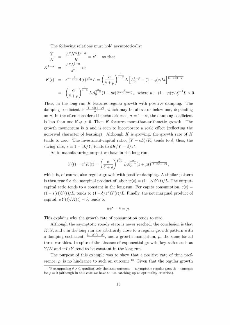
The following relations must hold asymptotically:

Y

K=

AσKαL1−α

K= z∗ so that

K1−α =AσL1−α

z∗or

K(t) = z∗−1

1−αA(t)σ

1−αL =

µα

δ + ρ

¶ 11−α

LhA1−ϕ0 + (1− ϕ)γLt

i σ(1−α)(1−ϕ)

=

µα

δ + ρ

¶ 11−α

LAσ

1−α0 (1 + μt)

σ(1−α)(1−ϕ) , where μ ≡ (1− ϕ)γAϕ−1

0 L > 0.

Thus, in the long run K features regular growth with positive damping. The

damping coefficient is (1−α)(1−ϕ)σ , which may be above or below one, depending

on σ. In the often considered benchmark case, σ = 1−α, the damping coefficient

is less than one if ϕ > 0. Then K features more-than-arithmetic growth. The

growth momentum is μ and is seen to incorporate a scale effect (reflecting the

non-rival character of learning). Although K is growing, the growth rate of K

tends to zero. The investment-capital ratio, (Y − cL)/K, tends to δ; thus, the

saving rate, s ≡ 1− cL/Y, tends to δK/Y = δ/z∗.

As to manufacturing output we have in the long run

Y (t) = z∗K(t) =

µα

δ + ρ

¶ α1−α

LAσ

1−α0 (1 + μt)

σ(1−α)(1−ϕ) ,

which is, of course, also regular growth with positive damping. A similar pattern

is then true for the marginal product of labor w(t) = (1−α)Y (t)/L. The output-

capital ratio tends to a constant in the long run. Per capita consumption, c(t) =

(1− s(t))Y (t)/L, tends to (1− δ/z∗)Y (t)/L. Finally, the net marginal product of

capital, αY (t)/K(t)− δ, tends to

αz∗ − δ = ρ.

This explains why the growth rate of consumption tends to zero.

Although the asymptotic steady state is never reached, the conclusion is that

K, Y, and c in the long run are arbitrarily close to a regular growth pattern with

a damping coefficient, (1−α)(1−ϕ)σ , and a growth momentum, μ, the same for all

three variables. In spite of the absence of exponential growth, key ratios such as

Y/K and wL/Y tend to be constant in the long run.

The purpose of this example was to show that a positive rate of time pref-

erence, ρ, is no hindrance to such an outcome.18 Given that the regular growth18Presupposing δ > 0, qualitatively the same outcome − asymptotic regular growth − emerges

for ρ = 0 (although in this case we have to use catching-up as optimality criterion).

15

pattern was inherited from the independent technology path described by (16),

this conclusion is perhaps no surprise. In the next section we consider an example

where there is mutual dependence between the development of technology and

the remainder of the economy.

5 Example 3: Investment-specific learning and em-bodied technical change

Motivated by the steady decline of the relative price of capital equipment and

the secular rise in the ratio of new equipment investment to GNP, Greenwood

et al. (1997) developed a tractable model with embodied technical change. The

framework has afterwards been applied and extended in different directions. One

such application is that of Boucekkine et al. (2003).19 They show that a relative

shift from general to investment-specific learning externalities may explain the

simultaneous occurrence of a faster decline in the price of capital equipment and

a productivity slowdown in the 1970s after the first oil price shock.

In this section we present a related model and show that regular, but less-than-

exponential growth may arise. To begin with we allow for population growth in

order to clarify the role of this aspect for the long-run results. Notation is as

above, unless otherwise indicated. The technology of the economy is described by

Y = KαL1−α, 0 < α < 1, (23)

K = qI − δK, δ > 0, K(0) = K0 given, (24)

q = γ

µZ t

−∞I(τ)dτ

¶β

, γ > 0, 0 < β < (1− α)/α, q(0) = q0 given, (25)

where L = L0ent, n ≥ 0, and K0, q0, and L0 are positive. The new variables are

I ≡ Y − cL, i.e., gross investment, and q which denotes the quality (productivity)of newly produced investment goods. There is learning by investing, but new

learning is incorporated only in newly produced investment goods (this is the

embodiment hypothesis). Thus, over time each new investment good gives rise to

a greater and greater addition to the capital stock, K, measured in constant

efficiency units. The quality q of investment goods of the current vintage is

determined by cumulative aggregate gross investment as indicated by (25). The

parameter β is named the “learning parameter”. The upper bound on β is brought

in to avoid explosive growth (infinite output in finite time). We assume capital

19We are thankful to Solow for suggesting that embodied technical change might fit our ap-proach and to a referee for suggesting in particular a look at the Boucekkine et al. (2003)paper.

16

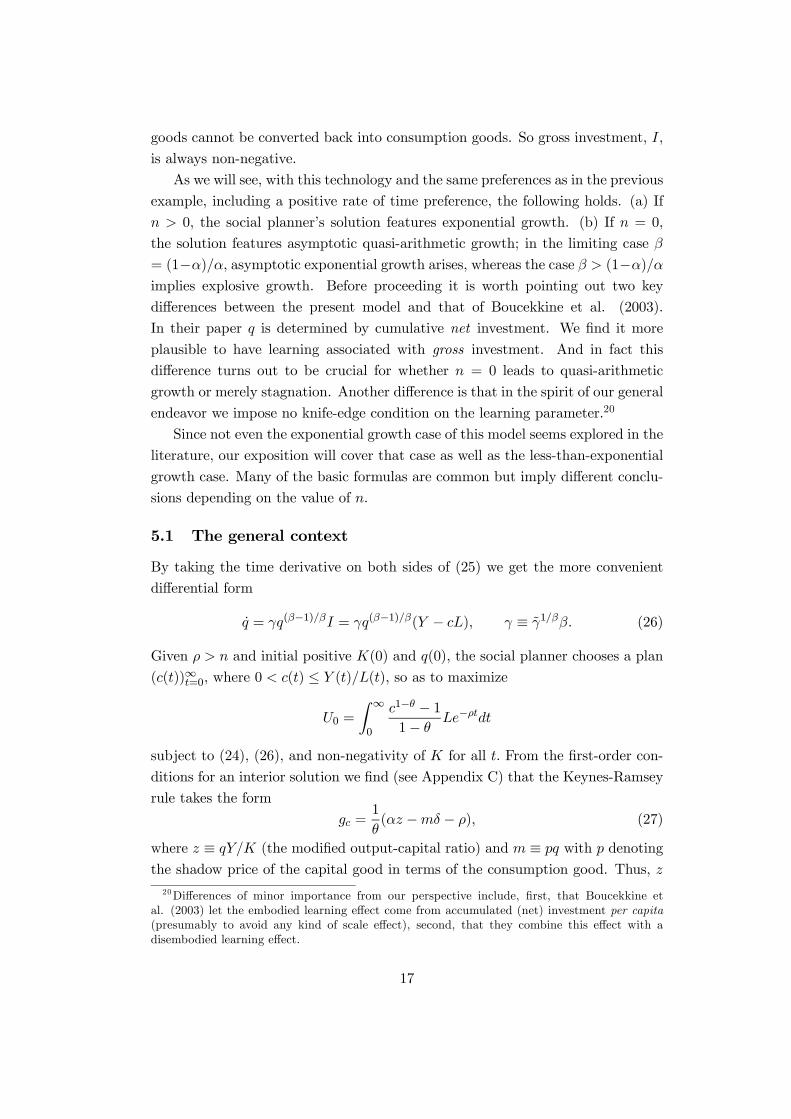
goods cannot be converted back into consumption goods. So gross investment, I,

is always non-negative.

As we will see, with this technology and the same preferences as in the previous

example, including a positive rate of time preference, the following holds. (a) If

n > 0, the social planner’s solution features exponential growth. (b) If n = 0,

the solution features asymptotic quasi-arithmetic growth; in the limiting case β

= (1−α)/α, asymptotic exponential growth arises, whereas the case β > (1−α)/αimplies explosive growth. Before proceeding it is worth pointing out two key

differences between the present model and that of Boucekkine et al. (2003).

In their paper q is determined by cumulative net investment. We find it more

plausible to have learning associated with gross investment. And in fact this

difference turns out to be crucial for whether n = 0 leads to quasi-arithmetic

growth or merely stagnation. Another difference is that in the spirit of our general

endeavor we impose no knife-edge condition on the learning parameter.20

Since not even the exponential growth case of this model seems explored in the

literature, our exposition will cover that case as well as the less-than-exponential

growth case. Many of the basic formulas are common but imply different conclu-

sions depending on the value of n.

5.1 The general context

By taking the time derivative on both sides of (25) we get the more convenient

differential form

q = γq(β−1)/βI = γq(β−1)/β(Y − cL), γ ≡ γ1/ββ. (26)

Given ρ > n and initial positive K(0) and q(0), the social planner chooses a plan

(c(t))∞t=0, where 0 < c(t) ≤ Y (t)/L(t), so as to maximize

U0 =

Z ∞

0

c1−θ − 11− θ

Le−ρtdt

subject to (24), (26), and non-negativity of K for all t. From the first-order con-

ditions for an interior solution we find (see Appendix C) that the Keynes-Ramsey

rule takes the form

gc =1

θ(αz −mδ − ρ), (27)

where z ≡ qY/K (the modified output-capital ratio) and m ≡ pq with p denoting

the shadow price of the capital good in terms of the consumption good. Thus, z20Differences of minor importance from our perspective include, first, that Boucekkine et

al. (2003) let the embodied learning effect come from accumulated (net) investment per capita(presumably to avoid any kind of scale effect), second, that they combine this effect with adisembodied learning effect.

17

is a modified output-capital ratio and m is the shadow price of newly produced

investment goods in terms of the consumption good. Let v ≡ qcL/K (the modified

consumption-capital ratio), so that, by (24), the growth rate ofK is gK = z−v−δ.Further, let h ≡ γY/q1/β, so that, by (26), the growth rate of q is gq = (1−v/z)h;that is, 1 − v/z is the saving rate, which we will denote s, and h is the highest

possible growth rate of the quality of newly produced investment goods. Then,

combining the first-order conditions and the dynamic constraints (24) and (26)

yields the dynamic system:

m =

∙1−m

m(δm− αz) + (1− v

z)h

¸m, (28)

v =

∙1

θ(αz − δm− ρ)− (z − v − δ − n) + (1− v

z)h

¸v, (29)

z =h−(1− α)(z − v − δ − n) + (1− v

z)hiz, (30)

h =

∙α(z − v − δ − n) + n− 1

β(1− v

z)h

¸h. (31)

Consider a steady state, (m∗, v∗, z∗, h∗), of this system. In steady state, if

n > 0, the economy follows a balanced growth path (BGP for short) with constant

growth rates of K, q, Y, and c. Indeed, from (30) and (31) we find the growth rate

of K to be

g∗K = z∗ − v∗ − δ =(1− α)(1 + β)

1− α(1 + β)n > n iff n > 0. (32)

The inequality is due to the parameter condition

α < 1/(1 + β) (33)

which is equivalent to β < (1− α)/α, the condition assumed in (25). Then, from

(30),

g∗q = s∗h∗ = (1− v∗

z∗)h∗ =

(1− α)β

1− α(1 + β)n =

β

1 + βg∗K . (34)

In view of constancy of h ≡ γY/q1/β,

g∗Y =1

βg∗q =

1

1 + βg∗K . (35)

That is, owing to the embodiment of technical progress Y does not grow as fast

as K. This is in line with the empirical evidence mentioned above. Inserting (27),

(32), and (34) into (29) we find

g∗c =1

θ(αz∗ −m∗δ − ρ) =

αβ

1− α(1 + β)n > 0 iff n > 0. (36)

18

This result is of course also obtained if we use constancy of v∗/z∗ to conclude that

g∗c = g∗Y − n. To ensure boundedness of the discounted utility integral we impose

the parameter restriction

(1− θ)αβ

1− α(1 + β)n < ρ− n, (37)

which is equivalent to (1− θ)g∗c < ρ− n.

With these findings we get from (28)

m∗ =α(θg∗c + ρ)

(1− α+ αθ)g∗c + αρ=

θαβn+ [1− α(1 + β)] ρ

(1− α+ αθ)n+ [1− α(1 + β)] ρ≤ 1, (38)

if n ≥ 0, respectively. The parameter restriction (37) implies m∗ > α. Next, from

(36),

z∗ =θβ

1− α(1 + β)n+

ρ+ δm∗

α> 0, (39)

so that, from (32),

v∗ =θβ − (1− α)(1 + β)

1− α(1 + β)n+

ρ+ δm∗

α− δ, (40)

and

s∗ ≡ 1− v∗

z∗= α

(1− α)(1 + β)n+ [1− α(1 + β)] δ

θαβn+ [1− α(1 + β)] (ρ+ δm∗)∈ (0, 1). (41)

That s∗ > 0 is immediate from the formula. And s∗ < 1 is implied by v∗ < z∗,

which immediately follows by comparing (40) and (39). Finally, we have from

(34)

h∗ =g∗qs∗=

(1− α)βn

[1− α(1 + β)] s∗≥ 0 for n ≥ 0, (42)

respectively.

In a BGP the shadow price p (≡ m/q) of the capital good in terms of the

consumption good is falling since m is constant while q is rising. Indeed,

g∗p = −g∗q = −(1− α)β

1− α(1 + β)n = − β

1 + βg∗K . (43)

Thus, at the same time as Y/K is falling, the value capital-output ratio Y/(pK)

stays constant in a BGP. If r denotes the social planner’s marginal net rate of

return in terms of the consumption good, we have r = [∂Y/∂K − (pδ − p)] /p.

Since p ≡ m/q and z ≡ qY/K, we have (∂Y/∂K)/p = αY/(pK) = αz∗/m∗.

Along the BGP, therefore,

r∗ = αz∗

m∗− (δ − g∗p) =

θαβ

1− α(1 + β)n+ ρ = θg∗c + ρ, (44)

19

as expected. Since the investment good and the consumption good are produced

by the same technology, we can alternatively calculate r as the marginal net rate

of return to investment: r = (∂Y/∂K − pδ) ∂K/∂I = (αY/K − pδ)q. In the BGP

we then get r∗ = αz∗ − m∗δ, which according to (36) amounts to the same as

(44).

We have hereby shown that if the learning parameter satisfies (33), a steady

state of the dynamic system is feasible and features exponential semi-endogenous

growth if n > 0.21 On the other hand, violation of (33) combined with a positive

n implies a growth potential so enormous that a steady state of the system is

infeasible and growth tends to be explosive. But what if n = 0?

5.2 The case with zero population growth

With n = 0 the formulas above are still valid. As a result the growth rates

g∗K , g∗q , g

∗c , and g

∗p are all zero, whereas m

∗ = 1, z∗ = (ρ+δ)/α, v∗ = (ρ+δ)/α−δ,s∗ = αδ/(ρ+ δ) = δ/z∗, and h∗ = 0. By definition we have h ≡ γY/q1/β > 0 for

all t. So the vanishing value of h∗ tells us that the economic system can never

attain the steady state. We will now show, however, that the system converges

towards this steady state, which is therefore an asymptotic steady state.

When n = 0 and α < 1/(1 + β), we have from purely technological reasons

that limt→∞ h = 0 (for details, see Appendix C). This implies that for t→∞ the

dynamics of m, v, and z approach the simpler form

m = (1−m)(δm− αz),

v =

∙1

θ(αz − δm− ρ)− (z − v − δ)

¸v,

z = −(1− α)(z − v − δ)z.

The associated Jacobian is

J =

⎡⎣ ρ 0 0

− δθv∗ v∗ (αθ − 1)v∗

0 (1− α)z∗ −(1− α)z∗

⎤⎦ .This is block-triangular and so the eigenvalues are ρ and those of the lower right

2 × 2 sub-matrix of J. Note that this sub-matrix is identical to the Jacobian inthe learning-by-doing example of Section 4. Accordingly, its eigenvalues are of

opposite sign. Since m and v are jump variables and z is pre-determined, it

follows that the asymptotic steady state is locally saddle-point stable.22

21The standard transversality conditions are satisfied at least if θ ≥ 1 (see Appendix C).Owing to non-concavity of the maximized Hamiltonian, however, we have not been able toestablish sufficient conditions for optimality.22The unique converging path unconditionally satisfies the standard transversality conditions,

see Appendix C.

20

For t → ∞ we therefore have s ≡ 1 − v/z → 1 − v∗/z∗ ≡ s∗ and K →L(q/z∗)1/(1−α) (from the definition of z). So, from (26) and (23) follows that

ultimately

q = γqβ−1β s∗KαL1−α = γLs∗z∗

−α1−α q

1−1−α(1+β)(1−α)β ≡ Cq1−ξ, (45)

where C and ξ are implicitly defined constants. This Bernoulli equation has the

solution

q(t) = (qξ0 + ξCt)1ξ = q0(1 + μt)

1ξ , where μ ≡ ξLγδ

µα

ρ+ δ

¶ 11−α

q−ξ0 ,

using the solutions for s∗ and z∗ above. This shows that in the long run the

productivity of newly produced investment goods features regular growth with

damping coefficient ξ = [1− α(1 + β)] / [(1− α)β] > 0 and growth momentum μ

(which, as expected, is seen to incorporate a scale effect reflecting the non-rival

character of learning). The corresponding long-run path for capital is

K(t) = L³ q

z∗

´ 11−α

= L

µα

ρ+ δ

¶ 11−α

q1

1−α0 (1 + μt)

1(1−α)ξ

and for output

Y (t) = K(t)αL1−α = L

µα

ρ+ δ

¶ α1−α

qα

1−α0 (1 + μt)

α(1−α)ξ .

The damping coefficient for Y is thus (1− α)ξ/α = [1− α(1 + β)] /(αβ), so that

more-than-arithmetic growth arises if 12(1−α)/α < β < (1−α)/α and less-than-

arithmetic growth if β is beneath the lower end of this interval. The same is then

true for the marginal product of labor, w(t) = (1− α)Y (t)/L, and for per capita

consumption, c(t) = (1− s(t))Y (t)/L, which tends to (1− δ/z∗)Y (t)/L. For the

capital-output ratio we ultimately have K(t)/Y (t) = q(t)/z∗, which implies more-

than-arithmetic growth if β > 1−α and less-than-arithmetic growth if β < 1−α.A new interesting facet compared with the learning-by-doing example of Sec-

tion 4 is that the shadow price, p, of capital goods remains falling, although at

a decreasing rate. This follows from the fact that the shadow price, m ≡ pq, of

newly produced investment goods in terms of the consumption good tends to a

constant at the same time as q is growing, although at a decreasing rate. Finally,

the value output-capital ratio Y/(pK) tends to the constant (qY/K)m = z∗m∗ =

z∗ = (ρ + δ)/α and the marginal net rate of return to investment tends to r∗

= αY/(pK)− δ = ρ.

These results hold when, in addition to n = 0, we have α < 1/(1 + β). In

the limiting case, α = 1/(1 + β), the growth formulas above no longer hold and

21

instead exponential growth arises. Indeed, the system (28), (29), (30), and (31)

is still valid and so is (45) in a steady state of the system. But now ξ = 0. We

therefore have in a steady state that q = Cq, which has the solution q(t) = q0eCt,

where C ≡ γLs∗z∗−α1−α > 0. By constancy of h in the steady state, gY = αgK

= gq/β = C/β = αC/(1 − α) so that also Y and K grow exponentially. This is

the fully-endogenous growth case of the model. If instead α > 1/(1 + β) we get

ξ < 0 in (45), implying explosive growth, a not plausible scenario.

We conclude this section with a remark on why, when exponential growth can-

not be sustained in a model, sometimes quasi-arithmetic growth results and some-

times complete stagnation. In the present context, where we focus on learning, it

is the source of learning that matters. Suppose that, contrary to our assumption

above, learning is associated with net investment, as in Boucekkine et al. (2003).

If with respect to the value of the learning parameter we rule out both the knife-

edge case leading to exponential growth and the explosive case, then n = 0 will

lead to complete stagnation. Even if there is an incentive to maintain the capital

stock, this requires no net investment and so learning tends to stop. When learn-

ing is associated with gross investment, however, maintaining the capital stock

implies sustained learning. In turn, this induces more investment than needed to

replace wear and tear and so capital accumulates, although at a declining rate.

Even if there are diminishing marginal returns to capital, this is countervailed

by the rising productivity of investment goods due to learning. Similarly, in the

learning-by-doing example of Section 4, where learning is simply associated with

working, learning occurs even if the capital stock is just maintained. Therefore,

instead of mere stagnation we get quasi-arithmetic growth.

6 Conclusion

The search for exponential growth paths can be justified by analytical simplicity

and the approximate constancy of the long-run growth rate for more than a cen-

tury in, for example, the US. Yet this paper argues that growth theory needs a

more general notion of regularity than that of exponential growth. We suggest

that paths along which the rate of decline of the growth rate is proportional to the

growth rate itself deserve attention; this criterion defines our concept of regular

growth. Exponential growth is the limiting case where the factor of proportional-

ity, the “damping coefficient”, is zero. When the damping coefficient is positive,

there is less-than-exponential growth, yet this growth exhibits a certain regularity

and is sustained in the sense that Y/L → ∞ for t → ∞. We believe that sucha broader perspective on growth will prove particularly useful for discussions of

the prospects of economic growth in the future, where population growth (and

22

thereby the expansion of the ultimate source of new ideas) is likely to come to an

end.

The main advantages of the generalized regularity concept are as follows: (1)

The concept allows researchers to reduce the number of problematic parameter

restrictions, which underlie both standard neoclassical and endogenous growth

models. (2) Since the resulting dynamic process has one more degree of freedom

compared to exponential growth, it is at least as plausible in empirical terms.

(3) The concept covers a continuum of sustained growth processes which fill the

whole range between exponential growth and complete stagnation, a range which

may deserve more attention in view of the likely future demographic development

in the world. (4) As our analyses of zero population growth in the Jones (1995)

model, a learning-by-doing model, and an embodied technical change model show,

falling growth rates need not mean that economic development grinds to a halt.

(5) Finally, at least for these three examples we have demonstrated not only the

presence of the generalized regularity pattern, but also the asymptotic stability

of this pattern.

The examples considered are based on a representative agent framework. Our

conjecture is that with heterogeneous agents the generalized notion of regular

growth could be of use as well. Likewise, an elaboration of the embodied tech-

nical change approach of Section 5 might be of empirical interest. For example,

Solow (1996) indicates that vintage effects tend to be more visible against a back-

ground of less-than exponential growth. As Solow has also suggested,23 there is an

array of “behavioral” assumptions waiting for application within growth theory,

in particular growth theory without the straightjacket of exponential growth.

7 Appendix

A. The canonical Ramsey example This appendix derives the results re-

ported for Case 4 in Section 3. The Hamiltonian for the optimal control problem

is:

H(K,A, c, u, λ1, λ2, t) =c1−θ − 11− θ

L+ λ1(Y − cL) + λ2γAϕ(1− u)L,

where Y = AσKα(uL)1−α and λ1 and λ2 are the co-state variables associated with

physical capital and knowledge, respectively. Applying the catching-up optimality

criterion, necessary first-order conditions (see Seierstad and Sydsaeter, 1987, p.

23Private communication.

23

232-34) for an interior solution are:

∂H

∂c= c−θL− λ1L = 0, (46)

∂H

∂u= λ1(1− α)

Y

u− λ2γA

ϕL = 0, (47)

∂H

∂K= λ1α

Y

K= −λ1, (48)

∂H

∂A= λ1σ

Y

A+ λ2ϕγA

ϕ−1(1− u)L = −λ2. (49)

Combining (46) and (48) gives the Keynes-Ramsey rule

gc =1

θαAσKα−1(uL)1−α. (50)

Given the definition p = λ2/λ1, (47), (48), and (49) yield

gp = αAσKα−1(uL)1−α − σγAϕ−1uL

1− α− ϕγAϕ−1(1− u)L. (51)

Let x ≡ pA/K. Log-differentiating x w.r.t. time and using (47), (6), (5), and (4)

gives (7). Log-differentiating (47) w.r.t. time, using (51), (5), (4) and (6), gives

(8). Finally, log-differentiating 1 − s ≡ cL/Y, using (50), (4), (6) and (5), gives

(9).

In the text we defined μ ≡ (1− ϕ)γ(1− u∗)LA0ϕ−1.

Lemma 1. In a steady state of the system (7), (8), and (9)

λ1(t)K(t) = λ1(0)K0(1 + μt)ω, and (52)

λ2(t)A(t) = λ2(0)A0(1 + μt)ω, (53)

where

ω ≡ σ + 1− ϕ− θ [σ + α(1− ϕ)]

(1− α)(1− ϕ).

Proof. As shown in the text, in a steady state of the system we have Y (t)/K(t)

= (Y (0)/K0)(1 + μt)−1 so thatZ t

0

Y (τ)

K(τ)dτ =

Y (0)

K0μ−1 ln(1 + μt) =

θ [σ + α(1− ϕ)]

α(1− α)(1− ϕ)ln(1 + μt),

where the latter equality follows from (13), (11), (10), and the definition of μ.

Therefore, by (48) and (13),

λ1(t)K(t) = λ1(0)e−α t

0Y (τ)K(τ)

dτK0(1 + μt)

σ+1−ϕ(1−α)(1−ϕ)

= λ1(0)K0(1 + μt)σ+1−ϕ

(1−α)(1−ϕ)−θ[σ+α(1−ϕ)](1−α)(1−ϕ) ,

24

which proves (52).

From (49) and p ≡ λ2/λ1 follows that in steady state

λ2λ2= −σY

pA− ϕγAϕ−1(1− u∗)L = −γ

µσu∗

1− α+ ϕ(1− u∗)

¶LAϕ−1

0 (1 + μt)−1,

where the latter equality follows from (4), (12), and (11). Hence,Z t

0

λ2(τ)

λ2(τ)dτ = −ϕ− σ − α+ θ [σ + α(1− ϕ)]

(1− α)(1− ϕ)ln(1 + μt),

by (10) and the definition of μ. Therefore,

λ2(t)A(t) = λ2(0)et0λ2(τ)λ2(τ)

dτA0(1+μt)

11−ϕ = λ2(0)A0(1+μt)

11−ϕ−

ϕ−σ−α+θ[σ+α(1−ϕ)](1−α)(1−ϕ) ,

which proves (53). ¤

We have ω < 0 if and only if

θ > (σ + 1− ϕ)/ [σ + α(1− ϕ)] . (54)

Hence, by Lemma 1 follows that the “standard” transversality conditions, limt→∞λ1(t)K(t) = 0 and limt→∞ λ2(t)A(t) = 0, hold along the unique regular growth

path if and only if (54) is satisfied. This condition is a little stronger than θ > 1.

Our conjecture is that these transversality conditions together with the first-order

conditions are necessary and sufficient for an optimal solution. This guessed

necessity and sufficiency is based on the saddle-point stability of the steady state

(see below). Yet, we have so far no proof. The maximized Hamiltonian is not

jointly concave in (K,A) unless σ = ϕ(1−α). Thus, the Arrow sufficiency theoremdoes not apply; hence, neither does the Mangasarian sufficiency theorem (see

Seierstad and Sydsaeter, 1987). So, we only have a conjecture. (This is of course

not a satisfactory situation, but we might add that this situation is quite common

in the semi-endogenous growth literature, although authors are often silent about

the issue.)

As to the stability question it is convenient to transform the dynamic system.

We do that in two steps. First, let z ≡ xu and q ≡ (1 − s)xu. Then the system

(7), (8), and (9) becomes:

z = γLAϕ−1³1− ϕ+

σ

α− z − (1− ϕ)u

´z,

u = γLAϕ−1µσ

α+

σ

1− αu− q

1− α

¶u,

q = γLAϕ−1µ1− ϕ+

α− θ

(1− α)θz − (1− ϕ)u+

1

1− αq

¶q.

25

The steady state of this system is (z∗, u∗, q∗) = (x∗u∗, u∗, (1 − s∗)x∗u∗). Second,

this system can be converted into an autonomous system in “transformed time”

τ = lnA(t) ≡ f(t). With u(t) < 1, f 0(t) = γA(t)ϕ−1(1 − u(t))L > 0 and we

have t = f−1(τ). Thus, considering z(τ) ≡ z(f−1(τ)), u(τ) ≡ u(f−1(τ)) and

q(τ) ≡ q(f−1(τ)), the above system is converted into:

dz

dτ=

³1− ϕ+

σ

α− z − (1− ϕ)u

´ z

1− u,

du

dτ=

µσ

α+

σ

1− αu− q

1− α

¶u

1− u,

dq

dτ=

µ1− ϕ+

α− θ

(1− α)θz − (1− ϕ)u+

1

1− αq

¶q

1− u.

The Jacobian of this system, evaluated in steady state, is

J =

⎡⎣ −z∗ −(1− ϕ)z∗ 00 σ

1−αu∗ − 1

1−αu∗

α−θ(1−α)θq

∗ −(1− ϕ)q∗ 11−αq

∗

⎤⎦ · 1

1− u∗.

The determinant is

detJ = −σθ + (θ − 1)(1− ϕ)α

(1− α)2θz∗u∗q∗ < 0,

in view of θ > 1. The trace is

trJ =(α− s∗)x∗ + σ

1− α

u∗

1− u∗=[σ + α(1− ϕ)] (2θ − 1)− σ − 1 + ϕ

(1− α)(θ − 1) [σ + α(1− ϕ)]

σu∗

1− u∗> 0,

in view of the transversality condition (54). Thus, J has one negative eigenvalue,

η1, and two eigenvalues with positive real part. All three variables, z, u and q,

are jump variables, but z and u are linked through

z =1− α

γLαAσ+1−ϕ(

u

K)1−α ≡ h(u, A,K). (55)

In order to check existence and uniqueness of a convergent solution, let x

= (x1, x2, x3) ≡ (z, u, q) and x = (x1, x2, x3) ≡ (z∗, u∗, q∗). Then, in a small neigh-borhood of x any convergent solution is of the form x(τ) = Cveη1τ + x, where C

is a constant, depending on initial A and K, and v = (v1, v2, v3) is an eigenvector

associated with η1 so that

(−z∗ − η1)v1 − (1− ϕ)z∗v2 = 0, (56a)

0 + (σ

1− αu∗ − η1)v2 −

1

1− αu∗v3 = 0, (56b)

α− θ

(1− α)θq∗v1 − (1− ϕ)q∗v2 + (

1

1− αq∗ − η1)v3 = 0. (56c)

26

We see that vi 6= 0, i = 1, 2, 3. Initial transformed time is τ0 = lnA0 and we

have x(τ0) = (h(u(0), A0,K0), u(0), q(0)) for A(0) = A0 and K(0) = K0 (both

pre-determined), where we have used (55) for t = 0. Hence, coordinate-wise,

x1(τ0) = Cv1eη1τ0 + z∗ = h(u(0), A0,K0), (57)

x2(τ0) = Cv2eη1τ0 + u∗ = u(0), (58)

x3(τ0) = Cv3eη1τ0 + q∗ = q(0). (59)

This system has a unique solution in (C,u(0), q(0)); indeed, substituting (58) and

(59) into (57), setting v1 = 1 and using z∗ = x∗u∗, gives

1

v2u(0) + u∗(x∗ − 1

v2) = h(u(0), A0,K0). (60)

It follows from Lemma 2 that, given θ > 1, (60) has a unique solution in u(0).

With the pre-determined initial value of the ratio, Aσ+1−ϕ/K1−α, in a small

neighborhood of its steady state value (which is γLαx∗u∗α/(1− α)), the solution

for u(0) is close to u∗, hence it belongs to the open interval (0, 1).

Lemma 2. Assume θ > 1. Then 1/v2 > x∗.

Proof. From (56a),

v2 =−z∗ − η1(1− ϕ)z∗

. (61)

Substituting v1 = 1 together with (56b) into (56c) gives

α− θ

(1− α)θq∗ − (1− ϕ)q∗v2 + (

1

1− αq∗ − η1)(σ −

(1− α)η1u∗

)v2 ≡ Q(v2, η1) = 0.

Replacing η1 and v2 in (61) by η and w(η), respectively, we see that P (η) ≡Q(w(η), η) is the characteristic polynomial of degree 3 corresponding to J . Now,

P (−z∗) = α− θ

(1− α)θq∗ < 0,

as θ > 1. Consider η0 ≡ −(1 − ϕ)z∗/x∗ − z∗ < −z∗. Clearly, w(η0) = 1/x∗.

If P (η0) > 0, then the unique negative eigenvalue η1 satisfies η0 < η1 < −z∗,implying that v2 ≡ w(η1) < 1/x∗, in view of w0(η) < 0; hence 1/v2 > x∗. It

remains to prove that P (η0) > 0. We have

P (η0) =α− θ

(1− α)θq∗ − (1− ϕ)q∗w(η0) + (

1

1− αq∗ − η1)(σ −

(1− α)η1u∗

)w(η0)

=α− θ

(1− α)θq∗ − (1− ϕ)q∗

x∗+ (

1

1− αq∗ − η0)(σ −

(1− α)η0u∗

)1

x∗

27

=α(1− θ) [(1− α)(1− ϕ) + σ] (1− s∗)x∗u∗

(1− α)θσ

+[(1− α)(1− ϕ) + σ] (1− s∗) + (1− α)σ

1− αu∗ +

1− ϕ

x∗σu∗ +

1− α

u∗x∗η20

=θ − 1θ

[σ + α(1− ϕ)] +1− α

u∗x∗η20 > 0,

where the third equality is based on reordering and the definition of q∗, whereas

the last equality is based on the formulas for x∗, u∗, and s∗ in (10); finally, the

inequality is due to θ > 1. ¤

B. The learning-by-doing example By (19), the transversality condition

(21) can be written

limt→∞

c(t)−θe−ρtK(t) = 0,

which is obviously satisfied along the asymptotic regular growth path, since ρ > 0,

and c and K feature less than exponential growth. In the text we claimed that

the first-order conditions together with the transversality condition are sufficient

for an optimal solution. Indeed, this follows from the Mangasarian sufficiency

theorem, since H is jointly concave in (K, c) and the state and co-state variables

are non-negative for all t ≥ 0, cf. Seierstad and Sydsaeter (1987, p. 234-35).

Uniqueness of the solution follows because H is strictly concave in (K, c) for all

t ≥ 0.

C. The investment-specific learning example The current-value Hamil-

tonian for the optimal control problem is:

H(K, q, c, λ1, λ2, t) =c1−θ − 11− θ

L+ λ1 [q(Y − cL)− δK] + λ2γqβ−1β (Y − cL),

where Y = KαL1−α and λ1 and λ2 are the co-state variables associated with

physical capital and the quality of newly produced investment goods, respectively.

An interior solution will satisfy the first-order conditions

∂H

∂c= c−θL− λ1qL− λ2γq

β−1β L = 0, (62)

∂H

∂K= λ1(qα

Y

K− δ) + λ2γq

β−1β α

Y

K= ρλ1 − λ1, (63)

∂H

∂q= λ1(Y − cL) + λ2γ

β − 1β

q−1β (Y − cL) = ρλ2 − λ2. (64)

The first-order conditions imply:

Lemma 3. ddt(c

−θ) = c−θ(ρ− αq YK ) + λ1qδ.

28

Proof. Let

u ≡ c−θ − λ1q = λ2γqβ−1β = λ2

q

I, (65)

by (62) and (26), respectively. Then, using (64) and I ≡ Y − cL,

gu = gλ2 +β − 1β

gq = ρ− (λ1λ2+ γ

β − 1β

q−1β )I +

β − 1β

γq−1β I = ρ− λ1

λ2I, (66)

so that

u = ρu− λ1λ2

Iu = ρu− λ1q, (67)

by (65). Rewriting (65) as c−θ = λ1q + u, we find

d

dt(c−θ) = λ1q + λ1q + u = ρu+ λ1q = ρc−θ − (ρλ1 − λ1)q (from (67) and (65))

= ρc−θ −∙(λ1q + λ2γq

β−1β )α

Y

K− λ1δ

¸q = ρc−θ − c−θαq

Y

K+ λ1qδ,

where the two latter equalities come from (63) and (62), respectively. ¤

From Lemma 3 follows

gc = −1

θ

ddt(c

−θ)

c−θ=1

θ(αz −mδ − ρ) ,

using that z ≡ qY/K and

m ≡ pq ≡ (λ1/c−θ)q =λ1

λ1q + λ2γqβ−1β

q, (68)

by (62). This proves (27).

The conjectured necessary and sufficient transversality conditions are limt→∞λ1(t)e

−ρtK(t) = 0 and limt→∞ λ2(t)e−ρtq(t) = 0. We now check whether these

conditions hold in the steady state. First, note that (63) and (65) give

gλ1 = ρ+ δ − c−θ

λ1αY

K= ρ+ δ − α

Y

pK= ρ+

1

m(mδ − αz)

= ρ− 1

m∗(θg∗c + ρ) =

(1− α+ αθ)g∗cα

in steady state, by (38). Further, we have in steady state g∗K = g∗c/α+ n. Hence,

g∗λ1 + g∗K − ρ = (1− θ)g∗c +n− ρ < 0, by the parameter restriction (37). Thus the

first transversality condition holds for all θ > 0.

From (66)

gλ2 + gq − ρ = ρ− λ1λ2

I − β − 1β

gq + gq − ρ = − m

1−mγq

−1β I +

1

βgq (by (68))

= − m

1−mgq +

1

βgq = −(θg∗c + ρ) +

1− α

αβg∗c =

1− α(1 + θβ)

1− α(1 + β)n− ρ,

29

in steady state, by (38), (34), and (36). It follows that θ ≥ 1 is sufficient for thesecond transversality condition to hold. If n = 0, no particular condition on θ is

needed to ensure this transversality condition.

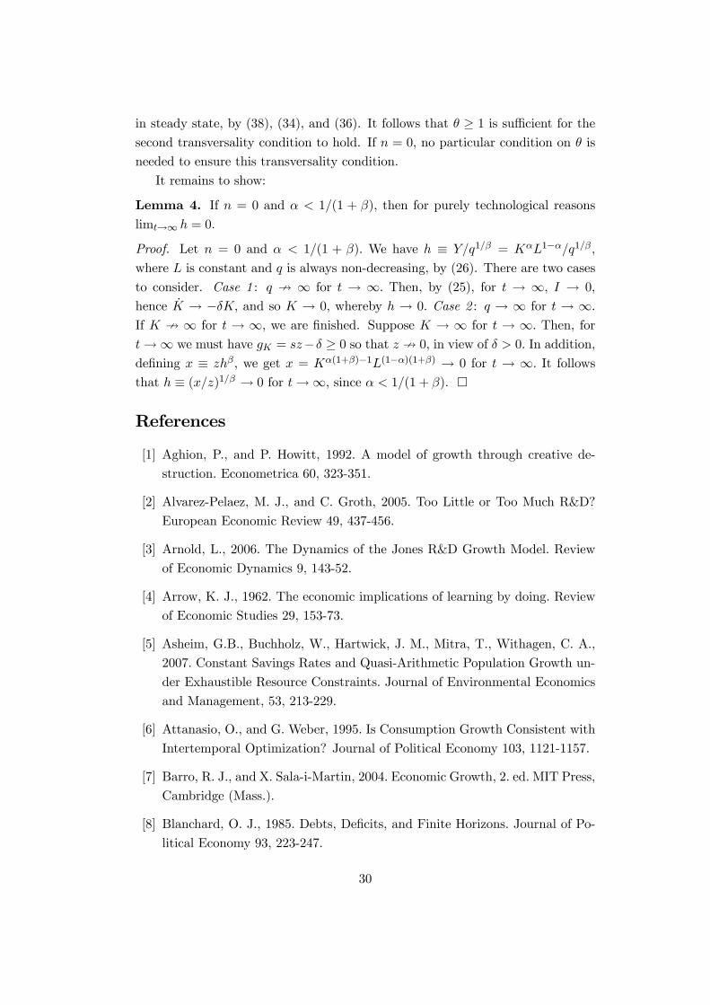
It remains to show:

Lemma 4. If n = 0 and α < 1/(1 + β), then for purely technological reasons

limt→∞ h = 0.

Proof. Let n = 0 and α < 1/(1 + β). We have h ≡ Y/q1/β = KαL1−α/q1/β ,

where L is constant and q is always non-decreasing, by (26). There are two cases

to consider. Case 1 : q 9 ∞ for t → ∞. Then, by (25), for t → ∞, I → 0,

hence K → −δK, and so K → 0, whereby h → 0. Case 2 : q → ∞ for t → ∞.

If K 9 ∞ for t → ∞, we are finished. Suppose K → ∞ for t → ∞. Then, for

t→∞ we must have gK = sz−δ ≥ 0 so that z 9 0, in view of δ > 0. In addition,

defining x ≡ zhβ, we get x = Kα(1+β)−1L(1−α)(1+β) → 0 for t → ∞. It follows

that h ≡ (x/z)1/β → 0 for t→∞, since α < 1/(1 + β). ¤

References

[1] Aghion, P., and P. Howitt, 1992. A model of growth through creative de-

struction. Econometrica 60, 323-351.

[2] Alvarez-Pelaez, M. J., and C. Groth, 2005. Too Little or Too Much R&D?

European Economic Review 49, 437-456.

[3] Arnold, L., 2006. The Dynamics of the Jones R&D Growth Model. Review

of Economic Dynamics 9, 143-52.

[4] Arrow, K. J., 1962. The economic implications of learning by doing. Review

of Economic Studies 29, 153-73.

[5] Asheim, G.B., Buchholz, W., Hartwick, J. M., Mitra, T., Withagen, C. A.,

2007. Constant Savings Rates and Quasi-Arithmetic Population Growth un-

der Exhaustible Resource Constraints. Journal of Environmental Economics

and Management, 53, 213-229.

[6] Attanasio, O., and G. Weber, 1995. Is Consumption Growth Consistent with

Intertemporal Optimization? Journal of Political Economy 103, 1121-1157.

[7] Barro, R. J., and X. Sala-i-Martin, 2004. Economic Growth, 2. ed. MIT Press,

Cambridge (Mass.).

[8] Blanchard, O. J., 1985. Debts, Deficits, and Finite Horizons. Journal of Po-

litical Economy 93, 223-247.

30

[9] Blanchard, O. J., Fischer, S., 1989. Lectures on Macroeconomics. MIT Press,

Cambridge MA.

[10] Boucekkine, R., F. del Rio, and O. Licandro, 2003. Embodied Technological

Change, Learning-by-doing and the Productivity Slowdown. Scandinavian

Journal of Economics 105 (1), 87-97.

[11] Dasgupta, P., Heal G., 1979. Economic Theory and Exhaustible Resources.

Cambridge University Press, Cambridge.

[12] Greenwood, J., Z. Hercowitz, and P. Krusell, 1997. Long-Run Implications

of Investment-Specific Technological Change. American Economic Review 87

(3), 342-362.

[13] Grossman, G. M., and E. Helpman, 1991. Innovation and Growth in the

Global Economy. MIT Press, Cambridge (Mass.).

[14] Growiec, J., 2007. Beyond the linearity critique: The knife-edge assumption

of steady-state growth. Economic Theory 31 (3), 489-499.

[15] Growiec, J., 2008, Knife-edge conditions in the modeling of long-run growth

regularities, Working Paper, Warsaw School of Economics.

[16] Hakenes, H., and A. Irmen, 2007, On the Long-run Evolution of Technological

Knowledge, Economic Theory 30, 171-180.

[17] Hartwick, J. M., 1977. Intergenerational Equity and the Investing of Rents

from Exhaustible Resources. American Economic Review 67, 972-974.

[18] Jones, C. I., 1995. R&D-based Models of Economic Growth. Journal of Po-

litical Economy 103, 759-784.

[19] Jones, C. I., 2005. Growth and Ideas. In: Handbook of Economic Growth,

vol. I.B, ed. by P. Aghion and S. N. Durlauf, Elsevier, Amsterdam, 1063-1111.

[20] Kremer, M., 1993. Population growth and technological change: One million

B.C. to 1990. Quarterly Journal of Economics 108, 681-716.

[21] McCallum, B. T., 1996. Neoclassical vs. endogenous growth analysis: An

overview. Federal Reserve Bank of Richmond Economic Quarterly Review

82, Fall, 41-71.

[22] Mitra, T., 1983. Limits on Population Growth under Exhaustible Resource

Constraints, International Economic Review 24, 155-168.

31

[23] Pezzey, J., 2004. Exact Measures of Income in a Hyperbolic Economy. Envi-

ronment and Development Economics 9, 473-484.

[24] Ramsey, F. P., 1928. A Mathematical Theory of Saving. The Economic Jour-

nal 38, 543-559.

[25] Romer, P. M., 1990. Endogenous Technological Change. Journal of Political

Economy 98, 71-101.

[26] Seierstad, A., Sydsaeter, K., 1987. Optimal Control Theory with Economic

Applications. North Holland, Amsterdam.

[27] Solow, R. M., 1974. Intergenerational Equity and Exhaustible Resources.

Review of Economic Studies, Symposium Issue, 29-45.

[28] Solow, R. M., 1994. Perspectives on Growth Theory. Journal of Economic

Perspectives 8, 45-54.

[29] Solow, R. M., 1996. Growth Theory without “Growth” − Notes Inspired byRereading Oelgaard. Nationaloekonomisk Tidsskrift − Festskrift til AndersOelgaard, 87-93.

[30] Solow, R. M., 2000. Growth Theory. An Exposition. Oxford University Press,

Oxford.

[31] United Nations, 2005. World Population Prospects. The 2004 Revision. New

York.

[32] Young, A., 1998. Growth without Scale Effects, Journal of Political Economy

106, 41-63.

32

Universität Leipzig Wirtschaftswissenschaftliche Fakultät Nr. 1 Wolfgang Bernhardt Stock Options wegen oder gegen Shareholder Value?

Vergütungsmodelle für Vorstände und Führungskräfte 04/98

Nr. 2 Thomas Lenk / Volkmar Teichmann Bei der Reform der Finanzverfassung die neuen Bundesländer nicht vergessen! 10/98

Nr. 3 Wolfgang Bernhardt Gedanken über Führen – Dienen – Verantworten 11/98

Nr. 4 Kristin Wellner Möglichkeiten und Grenzen kooperativer Standortgestaltung zur Revitalisie rung von Innenstädten 12/98

Nr. 5 Gerhardt Wolff Brauchen wir eine weitere Internationalisierung der Betriebswirtschaftslehre? 01/99

Nr. 6 Thomas Lenk / Friedrich Schneider Zurück zu mehr Föderalismus: Ein Vorschlag zur Neugestaltung des Finanz ausgleichs in der Bundesrepublik Deutschland unter besonderer Berücksichti- gung der neuen Bundesländer 12/98

Nr: 7 Thomas Lenk Kooperativer Förderalismus – Wettbewerbsorientierter Förderalismus 03/99

Nr. 8 Thomas Lenk / Andreas Mathes EU – Osterweiterung – Finanzierbar? 03/99

Nr. 9 Thomas Lenk / Volkmar Teichmann Die fisikalischen Wirkungen verschiedener Forderungen zur Neugestaltung des Länderfinanzausgleichs in der Bundesrepublik Deutschland: Eine empirische Analyse unter Einbeziehung der Normenkontrollanträge der Länder Baden-Würtemberg, Bayern und Hessen sowie der Stellungnahmen verschiedener Bundesländer 09/99

Nr. 10 Kai-Uwe Graw Gedanken zur Entwicklung der Strukturen im Bereich der Wasserversorgung unter besonderer Berücksichtigung kleiner und mittlerer Unternehmen 10/99

Nr. 11 Adolf Wagner Materialien zur Konjunkturforschung 12/99

Nr. 12 Anja Birke Die Übertragung westdeutscher Institutionen auf die ostdeutsche Wirklichkeit – erfolgversprechendes Zusammenspiel oder Aufdeckung systematischer Mängel?Ein empirischer Bericht für den kommunalen Finanzausgleich am Beispiel Sach02/00

Nr. 13 Rolf H. Hasse Internationaler Kapitalverkehr in den letzten 40 Jahren – Wohlstandsmotor oder Krisenursache? 03/00

Nr. 14 Wolfgang Bernhardt Unternehmensführung (Corporate Governance) und Hauptversammlung 04/00

Nr. 15 Adolf Wagner Materialien zur Wachstumsforschung 03/00

Nr. 16 Thomas Lenk / Anja Birke Determinanten des kommunalen Gebührenaufkommens unter besoBerücksichtigung der neuen Bundesländer 04/00

Nr. 17 Thomas Lenk Finanzwirtschaftliche Auswirkungen des Bundesverfassungsgerichtsurteils zum Länderfinanzausgleich vom 11.11.1999 04/00

Nr. 18 Dirk Bültel Continous linear utility for preferences on convex sets in normal real vector 05/00

Nr. 19 Stefan Dierkes / Stephanie Hanrath Steuerung dezentraler Investitionsentscheidungen bei nutzungsabhängigem und nutzungsunabhängigem Verschleiß des Anlagenvermögens 06/00

Nr. 20 Thomas Lenk / Andreas Mathes / Olaf Hirschefeld Zur Trennung von Bundes- und Landeskompetenzen in der Finanzverfassung Deutschlands 07/00

Nr. 21 Stefan Dierkes Marktwerte, Kapitalkosten und Betafaktoren bei wertabhängiger Finanzierung 10/00

Nr. 22 Thomas Lenk Intergovernmental Fiscal Relationships in Germany: Requirement forRegulations? 03/01

Nr. 23 Wolfgang Bernhardt Stock Options – Aktuelle Fragen Besteuerung, Bewertung, Offenlegung 03/01

Nr. 24 Thomas Lenk Die „kleine Reform“ des Länderfinanzausgleichs als Nukleus für die Finanzverfassungsreform“? 10/01

Nr. 25 Wolfgang Bernhardt Biotechnologie im Spannungsfeld von Menschenwürde, Forschung, Markt und Moral Wirtschaftsethik zwischen Beredsamkeit und Schweigen 11/01

2

Nr. 26 Thomas Lenk Finanzwirtschaftliche Bedeutung der Neuregelung des bundestaatlichen

Finanzausgleichs - Eine allkoative und distributive Wirkungsanalyse für das Jahr 2005 11/01

Nr. 27 Sören Bär Grundzüge eines Tourismusmarketing, untersucht für den Südraum Leipzig 05/02

Nr. 28 Wolfgang Bernhardt Der Deutsche Corporate Governance Kodex: Zuwahl (comply) oder Abwahl (explain)? 06/02

Nr. 29 Adolf Wagner Konjunkturtheorie, Globalisierung und Evolutionsökonomik 08/02

Nr. 30 Adolf Wagner Zur Profilbildung der Universitäten 08/02

Nr. 31 Sabine Klinger / Jens Ulrich / Hans-Joachim Rudolph

Konjunktur als Determinante des Erdgasverbrauchs in der ostdeutschen Industrie10/02

Nr. 32 Thomas Lenk / Anja Birke The Measurement of Expenditure Needs in the Fiscal Equalization at the LocaEmpirical Evidence from German Municipalities 10/02

Nr. 33 Wolfgang Bernhardt Die Lust am Fliegen Eine Parabel auf viel Corporate Governance und wenig Unternehmensführung 11/02

Nr. 34 Udo Hielscher Wie reich waren die reichsten Amerikaner wirklich? (US-Vermögensbewertungsindex 1800 – 2000) 12/02

Nr. 35 Uwe Haubold / Michael Nowak Risikoanalyse für Langfrist-Investments - Eine simulationsbasierte Studie – 12/02

Nr. 36 Thomas Lenk Die Neuregelung des bundesstaatlichen Finanzausgleichs – auf Basis der Steuerschätzung Mai 2002 und einer aktualisierten Bevölkerungsstatistik - 12/02

Nr. 37 Uwe Haubold / Michael Nowak Auswirkungen der Renditeverteilungsannahme auf Anlageentscheidungen - Eine simulationsbasierte Studie - 02/03

Nr. 38 Wolfgang Bernhard Corporate Governance Kondex für den Mittel-Stand? 06/03

Nr. 39 Hermut Kormann Familienunternehmen: Grundfragen mit finanzwirtschaftlichen Bezug 10/03

Nr. 40 Matthias Folk Launhardtsche Trichter 11/03

Nr. 41 Wolfgang Bernhardt Corporate Governance statt Unternehmensführung 11/03

Nr. 42 Thomas Lenk / Karolina Kaiser Das Prämienmodell im Länderfinanzausgleich – Anreiz- und Verteilungsmitwirk11/03

Nr. 43 Sabine Klinger Die Volkswirtschaftliche Gesamtrechnung des Haushaltsektors in einer Matrix 03/04

Nr. 44 Thomas Lenk / Heide Köpping Strategien zur Armutsbekämpfung und –vermeidung in Ostdeutschland: 05/04

Nr. 45 Wolfgang Bernhardt Sommernachtsfantasien Corporate Governance im Land der Träume. 07/04

Nr. 46 Thomas Lenk / Karolina Kaiser The Premium Model in the German Fiscal Equalization System 12/04

Nr. 47 Thomas Lenk / Christine Falken Komparative Analyse ausgewählter Indikatoren des Kommunalwirtschaft- lichen Gesamtergebnisses 05/05

Nr. 48 Michael Nowak / Stephan Barth Immobilienanlagen im Portfolio institutioneller Investoren am Beispiel von Versicherungsunternehmen -Auswirkungen auf die Risikosituation- 08/05

Nr. 49 Wolfgang Bernhardt Familiengesellschaften – Quo Vadis? Vorsicht vor zu viel „Professionalisierung“ und Ver-Fremdung 11/05

Nr. 50 Christian Milow Der Griff des Staates nach dem Währungsgold 12/05

Nr. 51 Anja Eichhorst / Karolina Kaiser The Instiutional Design of Bailouts and Its Role in Hardening Budget Constraints in Federations 03/06

Nr. 52 Ullrich Heilemann / Nancy Beck Die Mühen der Ebene – Regionale Wirtschaftsförderung in Leipzig 1991 bis 2004 08/06

Nr. 53 Gunther Schnabl Die Grenzen der monetären Integration in Europa 08/06

Nr. 54 Hermut Kormann Gibt es so etwas wie typisch mittelständige Strategien? 11/06

3

Nr. 55 Wolfgang Bernhardt (Miss-)Stimmung, Bestimmung und Mitbestimmung

Zwischen Juristentag und Biedenkopf-Kommission 11/06

Nr. 56 Ullrich Heilemann / Annika Blaschzik Indicators and the German Business Cycle - A Multivariate Perspective on Indicators of lfo, OECD, and ZEW 01/07

Nr. 57 Ullrich Heilemann “THE SOUL OF A NEW MACHINE” ZU DEN ANFÄNGEN DES RWI- KONJUNKTURMODELLS 12/06

Nr. 58 Ullrich Heilemann / Roland Schuhr / Annika Blaschzik

ZUR EVOLUTION DES DEUTSCHEN KONJUNKTURZYKLUS 1958 BIS 2004- ERGEBNISSE EINER DYNAMISCHEN DISKRIMINANZANALYSE 01/07

Nr. 59 Christine Falken / Mario Schmidt Kameralistik versus Doppik Zur Informationsfunktion des alten und neuen Rechnungswesens der Kommunen Teil I: Einführende und Erläuternde Betrach tungen zum Systemwechsel im kommunalen Rechnungswesen 01/07

Nr. 60 Christine Falken / Mario Schmidt Kameralistik versus Doppik Zur Informationsfunktion des alten und neuen Rechnungswesens der Kommunen Teil II Bewertung der Informationsfunktion im Vergleich 01/07

Nr. 61 Udo Hielscher MONTI DELLA CITTA DI FIRENZE Innovative Finanzierungen im Zeitalter Der Medici. Wurzeln der modernen Finanzmärkte 03/07

Nr. 62 Ullrich Heilemann / Stefan Wappler SACHSEN WÄCHST ANDERS - KONJUNKTURELLE; SEKTORALE UND REGIONALE BESTIMMUNGS GRÜNDE DER ENTWICKLUNG DER BRUTTOWERTSCHÖPFUNG 1992 BIS 2006 07/2007

Nr. 63 Adolf Wagner REGIONALÖKONOMIK: KONVERGIERENDE ODER DIVERGIERENDE REGIONALENTWICK- LUNGEN 08/2007

Nr. 64 Ullrich Heilemann / Jens Ulrich GOOD BYE; PROFESSOR PHILLIPS? ZUM WANDEL DER TARIFLOHNDETERMINANTEN IN DER BUNDESREPUBLIK 1952 – 2004 08/2007 Nr. 65 Gunther Schnabl / Franziska Schobert Monetary Policy Operations of Debtor Central Banks in MENA Countries 10/07 Nr. 66 Andreas Schäfer / Simone Valente Habit Formation, Dynastic Altruism, and Population Dynamics 11/07 Nr. 67 Wolfgang Bernhardt 5 Jahre Deutscher Corporate Governance Kondex Eine Erfolgsgeschichte? 01/2008 Nr. 68 Ullrich Heilemann / Jens Ulrich Viel Lärm um wenig? Zur Empirie von Lohnformeln in der Bundesrepublik 01/2008 Nr. 69 Christian Groth / Karl-Josef Koch / When economic growth is less than exponential Thomas M. Steger 02/2008