
Working Paper No. 2019-13 - University of Alberta
75
Working Paper No. 2019-13 Entry Preemption by Domestic Leaders and Home-Bias Patterns: Theory and Empirics Martin Alfaro University of Alberta September 2019 Copyright to papers in this working paper series rests with the authors and their assignees. Papers may be downloaded for personal use. Downloading of papers for any other activity may not be done without the written consent of the authors. Short excerpts of these working papers may be quoted without explicit permission provided that full credit is given to the source. The Department of Economics, the Institute for Public Economics, and the University of Alberta accept no responsibility for the accuracy or point of view represented in this work in progress.
Transcript of Working Paper No. 2019-13 - University of Alberta

Working Paper No. 2019-13
Entry Preemption by Domestic Leaders and Home-Bias Patterns:
Theory and Empirics
Martin Alfaro University of Alberta
September 2019 Copyright to papers in this working paper series rests with the authors and their assignees. Papers may be downloaded for personal use. Downloading of papers for any other activity may not be done without the written consent of the authors. Short excerpts of these working papers may be quoted without explicit permission provided that full credit is given to the source. The Department of Economics, the Institute for Public Economics, and the University of Alberta accept no responsibility for the accuracy or point of view represented in this work in progress.

Entry Preemption by Domestic Leaders andHome-Bias Patterns: Theory and Empirics∗
Martın Alfaro†
This Version: September 4, 2019
For the latest version, click here
Abstract
This paper studies a mechanism which arises through the strategic use of demand-
enhancing investments by domestic leaders. To accomplish this, I develop a parsimo-
nious framework that allows for firm heterogeneity, strategic interactions, multiple
choices, and extensive-margin adjustments. The mechanism is such that, relative
to a non-strategic benchmark, domestic leaders follow an overinvestment strategy
which preempts the entry of importers and increases their domestic sales. This gen-
erates greater concentration and home-bias patterns at both the firm and aggregate
level. The results are robust to the type of competition (i.e., prices or quantities) and
whether investments trigger increases or decreases in prices. Estimating the model
for Danish manufacturing industries, I show that, in industries with lower substi-
tutability, the strategic effect on concentration and domestic intensity is greater for
consumer goods, and lower regarding concentration for producer goods.
Keywords: domestic leaders, demand-enhancing investments, preemption, con-
centration, home bias.
JEL codes: F12, F14, L13, L6.
∗This paper is based on the second and third chapters of my Ph.D. dissertation. I especially thankRaymond Riezman, Philipp Schroder, and Valerie Smeets for their invaluable guidance and support. Ialso thank Peter Neary for acting as host during my visit at Oxford University where part of this researchhas been conducted. For useful comments, I thank Boris Georgiev, David Lander, Anders Laugesen,Kalina Manova, Allan Sørensen, Jim Tybout, and Frederic Warsynzki. I also thank Aarhus University forproviding me with access to Danish Data. Funding from University of Alberta is acknowledged.†University of Alberta, Department of Economics. 9-08 HM Tory Building, Edmonton, AB T6G 2H4,
Canada. Email: [email protected]. Link to my personal website.

1 Introduction 1
2 On Domestic Advantages and Strategic Moves 7
3 Empirical Facts 9
4 Setup 12
4.1 Supply Side . . . . . . . . . . . . . . . . . . . . . . . . . . . . . . . . . . . 14
4.2 Demand Side . . . . . . . . . . . . . . . . . . . . . . . . . . . . . . . . . . 15
5 Theoretical Analysis 17
5.1 Simultaneous Case . . . . . . . . . . . . . . . . . . . . . . . . . . . . . . . 18
5.2 Sequential Case . . . . . . . . . . . . . . . . . . . . . . . . . . . . . . . . . 20
5.3 Results . . . . . . . . . . . . . . . . . . . . . . . . . . . . . . . . . . . . . . 21
6 Taking the Model to the Data 23
6.1 Functional Forms . . . . . . . . . . . . . . . . . . . . . . . . . . . . . . . . 23
6.2 Counterfactual and Outcomes . . . . . . . . . . . . . . . . . . . . . . . . . 25
7 Empirical Analysis 26
7.1 Data Description . . . . . . . . . . . . . . . . . . . . . . . . . . . . . . . . 26
7.2 Definitions and Dataset . . . . . . . . . . . . . . . . . . . . . . . . . . . . . 27
7.3 Determination of Parameters . . . . . . . . . . . . . . . . . . . . . . . . . . 28
7.4 Results . . . . . . . . . . . . . . . . . . . . . . . . . . . . . . . . . . . . . . 29
8 Conclusions 33
ONLINE APPENDIX - NOT FOR PUBLICATION A-1
A Derivations and Proofs . . . . . . . . . . . . . . . . . . . . . . . . . . . . . A-1
B The Structural Model . . . . . . . . . . . . . . . . . . . . . . . . . . . . . . A-6
C Sample Determination and Estimation of δ . . . . . . . . . . . . . . . . . . A-16
D Empirical Features of Domestic Leaders . . . . . . . . . . . . . . . . . . . . A-19
E Additional Theoretical Results . . . . . . . . . . . . . . . . . . . . . . . . . A-20
F Additional Quantitative Results . . . . . . . . . . . . . . . . . . . . . . . . A-30

Martın Alfaro 1 INTRODUCTION
1 Introduction
In recent years, a surge of studies have raised concerns about the increase in concentration
and markups in some developed economies. The underlying causes which lead to these
outcomes, nonetheless, are not unique and might entail radically different policy interven-
tions. Thus, as emphasized by Berry et al. (2019), there is a need for more research on
how markets function in the modern economy and, as a corollary, on the determinants of
concentration. At the same time, other studies have remarked on home-bias phenomena in
open economies. Specifically, at an aggregate level, industries exhibit a tendency towards
consumption of domestic goods while, at the firm level, the share of a firm’s exports rela-
tive to its total sales tends to be less than its domestic portion. This phenomenon has been
considered by Obstfeld and Rogoff (2001) as one of the six major puzzles in International
Macroeconomics, and delving into the sources of trade barriers remains a key challenge
(Bernard et al., 2012; Chaney, 2014).
In this paper, I study theoretically and quantify a mechanism in which greater concen-
tration and home-bias patterns arise endogenously by the strategic behavior of domestic
firms. I conceive an environment in which firms make entry choices and, conditional on
being active, decide on prices and sunk expenditures which enhance demand as in Sutton
(1991,1998). These investments cover outlays on a wide range of variables, which all share
the property of boosting the firm’s quantity demanded and possibly entailing different
effects on prices. For instance, while quality upgrades could increase prices, investments
to reach low-valuation consumers (e.g., introducing inferior-quality products or improving
the distribution network) might decrease them.
The mechanism I posit has some key elements. First, following a vast literature in
International Business, I acknowledge that domestic firms have an advantage over those
which serve the market without being established where the buyer is. Furthermore, do-
mestic leaders (henceforth, DLs), defined as the firms with the greatest market share, are
in a position to exploit these advantages strategically: given their size in the market, they
are capable of shaping market conditions. In addition, I rely on an empirical fact that I
identify in my dataset (Stylized Fact 1 of this paper), where in a typical manufacturing
industry, DLs coexist with numerous firms that have insignificant domestic market shares.
In my model, all these elements are assembled in such a way that DLs sink investments
in their home market and force the negligible firms in the market (either domestic or
1

Martın Alfaro 1 INTRODUCTION
non-domestic) to condition their decisions on these expenditures.
To isolate the effects stemming from strategic motives to invest, I compare the situation
against a non-strategic benchmark, where rivals make decisions without conditioning on
DLs’ investments.1 Relative to that baseline, I show that DLs invest more heavily at
home, triggering a reallocation of domestic market shares towards them. This determines
the existence of two home-bias patterns. First, the expansion of DLs in their home market
is, in part, at the expense of the least-productive importers. This crowding out of foreign
competition creates an aggregate bias towards sales by domestic firms. In addition, the
greater domestic revenues of DLs increase their domestic intensity, defined as the firm’s
share of domestic sales relative to its total revenues. This last result is in line with an
empirical regularity that I identify in my dataset, presented as Stylized Fact 2 in this
paper, where DLs display a greater domestic bias relative to firms with negligible market
shares.
After presenting some remarks on the strategic exploitation of domestic advantages
(Section 2) and stating some empirical regularities (Section 3), I proceed to study the
mechanism theoretically in Section 4 and Section 5. Mainly, this attends to the usual
concern that results coming from oligopoly models can be subject to a lack of robustness.
When strategic interactions are incorporated, models might become quite sensitive to
specific details and have multiple equilibria. The concern turns to be especially acute
for the mechanism under study since, in typical two-stage oligopoly models with one
incumbent and one entrant, it has been shown that an overinvestment or underinvestment
pattern can emerge depending on whether the competition is a la Cournot or Bertrand.2
In my model, the overinvestment pattern arises irrespective of whether the competition
is on quantities or prices or, more generally, on strategic substitutes or complements. It
is also independent of whether investments provide incentives to the firm to increase or
decrease its prices, and even robust to an alternative where firms undertake cost-reducing
investments that are country specific. The key for this is that, unlike previous studies, I
incorporate the existence of an unbounded pool of entrants which are ready to enter if they
anticipate positive profits.3 This feature makes underinvestment strategies to accommo-
1The approach is standard in Game Theory to measure the strategic value of a strategy. In thatfield, the scenario in which rivals condition on the action under analysis is known as the closed-loopequilibrium, while the benchmark where rivals do not condition on it is referred to as the open-loopequilibrium (Fudenberg and Tirole, 1991).
2See, for instance, Tirole (1988).3A similar intuition, but where investments by domestic leaders are compared relative to investments
2

Martın Alfaro 1 INTRODUCTION
date entry unprofitable. The reason is that any excess of unexploited profits would trigger
entry and, therefore, undermine the original attempt to keep rents high. The mechanism
posited underscores tacit competition as an important determinant of market decisions
and ascribes a preemptive motive to the overinvestment strategy: DLs find it optimal to
expand sales that would otherwise be made by rival firms. This logic accords well with the
common idea in business of why big firms launch new products and persistently overhaul
goods, which can be summarized through the famous phrase by Steve Jobs that “if you
don’t cannibalize yourself, someone else will” (Isaacson, 2011).4
The incorporation of nonzero measure firms, heterogeneity, multiple choices, and en-
dogenous entry might introduce complex strategic interactions that turn the search for a
solution into an unwieldy task. This calls for building up a framework that incorporates
these features parsimoniously to, ultimately, be able to take the model to the data. I
accomplish this by adding two features to my setup. First, I consider a demand system
that allows me to describe the strategic interactions between firms through the theory
of Aggregative Games. This technique, recently put forward by Acemoglu and Jensen
(2013), is particularly well suited for setups with firm heterogeneity and multidimensional
strategies. Remarkably, it covers augmented versions of standard demand systems, includ-
ing those to tackle empirical questions.5 The second feature of the model comes from the
empirical fact mentioned above (Stylized Fact 1), which indicates that DLs coexist with
a myriad of firms that have trivial market shares. Based on this, I build a setup where a
fixed number of firms that are non-negligible in their home market are embedded into a
monopolistic competition model as in Melitz (2003).6 Remarkably, the model constitutes
a strict generalization of Melitz (2003) that collapses to it when either the number of DLs
by entrants, is present in Etro (2006).4Formal evidence of the use of demand-enhancing investments to preempt entry can be found in
Boulding and Christen (2009). They consider product lines as a choice variable. Paton (2008) does thesame for advertising as a decision choice by conducting an anonymous questionnaire to more than 800advertising managers of medium and large size UK-based firms. In the survey, a considerable portion ofmanagers view advertising as a strategic tool to be deployed in response to entry. Also, advertising is usedmore intensively by large firms and, consistent with my model, firms that are dominant in their marketsare significantly more likely to perceive advertising as a strategic instrument.
5For instance, it encompasses (possibly asymmetric) augmented versions of the CES, Logit, affinetranslations of these two, a linear demand, and a translog demand. In case that firms are multiproduct,it also encompasses the nested versions of the CES and Logit with each group defined by own firm’svarieties.
6Sutton (1991) shows that, when firms make choices on demand-enhancing investments, market con-centration is bounded away from zero. Thus, there is always at least one firm that is large and there canbe coexistence of leaders with firms having trivial market shares. Also, Shimomura and Thisse (2012) andParenti (2018), under homogeneity of firms within groups, consider a market structure with coexistenceof small and large firms.
3

Martın Alfaro 1 INTRODUCTION
is assumed to be zero or their effect on the market conditions is trivial.
Regarding the empirical side, with the aim of taking the model to the data, in Section
6 I turn the general framework into a structural model.7 The quantitative approach
is widely applicable since it only requires information on DLs’ market shares and the
determination of two parameters, with one of them being the elasticity of substitution. In
particular, information related to other firms is not needed, while information on prices is
only necessary for estimating parameters.
To study the mechanism, I draw on information from manufacturing industries in
Denmark. In Section 7, I describe the datasets at my disposal and remark on two features
of the data which make them suitable for the analysis. First, the information on domestic
firms is presented at the firm-product level. This allows me to allocate each firm-product
to a properly defined market and, hence, obtain the firm’s market share for each industry
where the firm is active. Second, the information on international transactions is also
presented at the firm-product level and encompasses imports by both manufacturing and
non-manufacturing firms. In this way, I am able to account for a proper measure of import
competition for each industry.
The results point out that strategic gains can be important determinants of the market
structure regarding concentration and firm’s domestic intensity. In addition, they also re-
veal a stark heterogeneity of outcomes. Nevertheless, arguably, magnitudes of estimations
coming from structural models should be interpreted with some caveats. The reason lies
in the simplifications and assumptions about unobservables to which they are subject. On
the other hand, they constitute a powerful tool for comparing the relative importance of
either two mechanisms within a group or, as in this paper, the same mechanism across
different groups.
To study how strategic motives to invest impact industries differently, I begin by per-
forming an analysis of the theoretical predictions. For the range of values observed in the
data, this indicates that the magnitude of outcomes depends mainly on the distributions
of market shares and domestic intensity. Specifically, industries are more impacted when
DLs command more market share and have sales well diversified across markets.8 Regard-
7The main reason to resort to a structural model is based on Sutton (1996). He argues that strategicasymmetries of the nature I study pose a limitation in any empirical analysis. Except for what hedenominates “happy accidents” (i.e., natural experiments), which are rarely if ever observed, strategicasymmetries should be considered as unobservables.
8From a theoretical point of view, while variations in market share and domestic intensity are positive,these increases are non-monotone. Nonetheless, when market shares are not disproportionately large and
4

Martın Alfaro 1 INTRODUCTION
ing the former, this is because when DLs have a low presence in the industry, they are less
capable of influencing the market conditions and, hence, gaining market share strategi-
cally. As for domestic intensity, if a firm sells almost exclusively at home, any increase in
domestic revenue has a trivial impact on the relative proportions of sales between domestic
and export markets.
Based on this, I make use of an empirical pattern that I identify in my dataset (Stylized
Fact 3 of this paper). The result provides me with some guidance for identifying the
industries where the deployment of strategic moves would have a more pronounced impact.
It states that the distributions of market shares and domestic intensity differ in industries
according to their good substitutability and the final user of the good (i.e., consumers
or producers).9 Specifically, in consumer goods, a greater substitution is associated with
lower concentration and greater domestic intensity. On the other hand, for producer
goods, industries with greater substitution are more concentrated, displaying statistically
insignificant differences in terms of domestic intensity.
Guided by this empirical fact, I corroborate that the outcomes in the structural model
differ by good substitutability and the final user of the good. As expected based on
the analysis outlined above, the results establish that, for consumer goods, increases in
concentration and domestic intensity are greater in industries with lower substitutability.
As for producer goods, there are greater concentration effects in industries with a higher
substitutability, and a statistically insignificant relation with domestic intensity.
Related Literature and Contributions. My paper contributes to different strands
of the literature. First, it touches upon studies which build up structural models incor-
porating large firms as key players in international economies.10 In general, these papers
suppose either a fixed number of firms or resort to ad hoc assumptions to model entry.11
Moreover, at a theoretical level, they obtain predictions under specific functional forms,
such as a CES demand. My contribution in this regard is developing a framework to study
theoretically and quantify phenomena with non-negligible firms. The setup is based on em-
DLs have sales skewed to their home market, as it happens in the Danish data, the model behaves asdescribed.
9Substitution is measured through the elasticity of substitution from Soderbery (2015), which is esti-mated following the procedure by Broda and Weinstein (2006) but corrected for small-sample biases. Inaddition, the classification by final user of the good corresponds to the BEC classification.
10For some recent literature, see, for instance, Atkeson and Burstein (2008), Eaton et al. (2012), Edmondet al. (2015), and Gaubert and Itskhoki (2018).
11For instance, Eaton et al. (2012) and Gaubert and Itskhoki (2018) assume that the number of firmsis a random variable.
5

Martın Alfaro 1 INTRODUCTION
pirical regularities and underscores Aggregative Games as a fruitful tool for incorporating
strategic interactions into empirical models. It can also be turned into a structural model
that incorporates strategic behavior while allowing for firm heterogeneity, extensive-margin
adjustments, and multidimensional strategies. In addition, the demand system allows for
different functional forms, while heterogeneity of large firms is not restricted to a specific
distribution. Remarkably, the approach constitutes a strict generalization of a model a la
Melitz (2003) such that, if all firms in an industry had negligible market shares, it would
generate the same results. Due to this, it improves upon structural estimations under this
variant of monopolistic competition where only atomistic firms are allowed.
My paper is also related to a growing literature that studies the impact on the economy
of the so-called superstar firms.12 In particular, there has been an ongoing debate about
the welfare consequences regarding the rise of concentration in the USA. In line with
Autor et al. (2017), my model underlines that reallocation of market share towards more
productive firms does not necessarily make consumers worse off. This holds even when
the outcomes depict a situation with more concentration, less international trade, and
possibly higher markups. Although general results are not possible to obtain theoretically,
the strategic behavior makes consumers better off under the assumptions of an augmented
CES (as in my structural model) and investments on non-price variables which are desirable
for the consumers (e.g., quality). This echoes the core intuition of market contestability
by Baumol et al. (1982): even when a concentrated market is observed, the threat of entry,
in opposition to actual entry, might discipline the incumbents in such a way that desirable
welfare outcomes emerge. Thus, my model highlights tacit competition as a potential
welfare-improving channel.
Finally, my paper relates to a literature that deals with home-bias patterns. After
McCallum’s (1995) border puzzle and Trefler’s (1995) mystery of missing trade, the great
bulk of studies with open economies have assumed the existence of trade costs as pa-
rameters that capture frictions between countries. Some other studies have generated
the phenomenon endogenously by resorting to explanations based on the supply nature
or preferences.13 By considering the preemptive strategies pursued by DLs, I focus on a
12See, for instance, Autor et al. (2017), De Loecker and Eeckhout (2017), Gutierrez and Philippon(2017), and De Loecker and Eeckhout (2018).
13Explanations based on the supply side can be found in, among others, Hillberry and Hummels (2002),Yi (2010), and Chaney (2014). Regarding reasons related to the demand side, there is a vast literatureresorting to a taste for national goods which goes back to at least Armington (1969). Also, Caron et al.(2014) propose a mechanism based on nonhomotheticities of preferences.
6

Martın Alfaro 2 ON DOMESTIC ADVANTAGES AND STRATEGIC MOVES
cause which, to the best of my knowledge, has not been explored before.
2 On Domestic Advantages and Strategic Moves
In a setting where firms are non-negligible in their own industry, the incorporation of
non-price choices expands the sources of strategic interactions and the possibilities that
firms have to achieve a better position in the market. As my results hinge on this line of
reasoning, I expand upon it in this section.
The formalization that the competition between firms is broader than the mere choice
of prices has been at the roots of the Industrial Organization literature since its inception.
In particular, Schelling (1960) argues that, in any game, once that it is recognized that
agents behave in a strategic way regarding their actions, it should also be acknowledged
that they behave strategically concerning the game itself. That is, if agents have the
opportunity, they do not take the rules of the game as given and make moves that alter
the original situation with the aim of achieving a better outcome. Schelling (1960) refers
to these actions as strategic moves. The idea has been applied to oligopolies in order to
explain non-price decisions made by incumbents with the aim of endogenously creating
market conditions favorable to them. As Porter (1998) points out, “successful firms not
only respond to their environment but also attempt to influence it in their favor”.
In tradable industries, domestic firms, defined as those which have established oper-
ations in the market to serve, enjoy certain potential advantages by being located where
the buyer is. It allows them to collect more and better information regarding the local
environment, react quicker to changes in market conditions, establish and maintain rela-
tions more easily with local intermediaries, and get a better grasp of customer tastes. In
addition, the superior knowledge of the market might improve the effectiveness of firms’
strategies if they are tailored to the idiosyncrasies of the country.14
In my setting, domestic firms are endowed with a strategic asymmetry which is ma-
terialized through sunk expenditures.15 By their sunk nature, these investments, once
incurred, cannot be recovered. Consequently, domestic firms that have the necessary size
14In the International Business literature, the fact that foreign firms are at a disadvantage is known as“liability of foreignness”. There is a vast literature on the subject which includes both theoretical andempirical studies. For a summary of the arguments see, for instance, Porter (1980, pp. 281-287; 2011,Chapter 3).
15The sunk nature of investments plays an important role. Otherwise, if costs were fixed but not sunk,the decisions could be reverted and the interaction would be better described by a setting with simulta-neous decisions. In terms of Schelling (1960), the sunk nature of costs turns decisions into commitments.
7

Martın Alfaro 2 ON DOMESTIC ADVANTAGES AND STRATEGIC MOVES
in the industry to influence market conditions are capable of committing resources in such
a way that competitors, and in particular smaller firms (either local or from abroad),
condition their choices on these investments.
Different variables have been considered in the literature as endogenous sunk expendi-
tures which enhance demand.16 By definition, they include any expenditure which boosts
firm demand in subsequent stages of the market. Thus, for instance, they include adver-
tisement, investments to broaden the line of goods, adaptation of products to consumers’
tastes, and investments on distribution channels that make the product more widely avail-
able.
Some remarks are in order in relation to this paper. First, the mechanism posited in
my model does not aim at explaining why a firm is an industry leader in the first place.
Rather, the focus is on how, conditional on being an important player in the industry, a
DL deploys strategies to improve its position in the market.
Second, I classify a firm as domestic if it has production activities within the country,
irrespective of their ownership or whether part of their home sales comes from imports.
This follows because the advantages I mentioned are acquired by “being in the market”.
On the other hand, pure importers (i.e., those that are not residing where the buyer is)
face additional difficulties of the type indicated above. This might prevent them from
succeeding in the market to the extent that they can get the presence necessary to emerge
as a player capable of setting the rules of that market. One way to overcome these hurdles
is establishing operations in the host country.17 The idea has been central in the theories of
multinational enterprises since, at least, the seminal works of Hymer (1960) and Dunning
(1977). Thus, the strategic gains also relate to the benefits that mature multinational
enterprises might reap from doing foreign direct investment.
Third, formally, the strategic motive to invest is captured in my model by an early
choice that generates a first-mover advantage. Nonetheless, the framework should be
conceived in terms of what rivals know and condition on when they choose a strategy,
rather than the timing itself. The intuition is the same as in the Prisoner’s Dilemma, or
16Firms might also have the possibility of sinking investments that affect marginal costs. My analysisapplies to this case if the cost advantages are country specific (see Appendix E.4). For instance, this arisesif a firm invests on distribution networks which reduce the marginal costs in that specific market.
17For an empirical study on the effects of foreign direct investment on profitability, see Cosar et al.(2018) for the car industry. This paper is particularly noteworthy given the richness of the data. Theyprovide evidence that establishing local assembly plants benefit firms more through the increases in thedemand that it entails rather than from savings on the cost side.
8

Martın Alfaro 3 EMPIRICAL FACTS
more generally the definition of static games: assumptions on timing are not necessarily
about the time at which a player makes a choice, but about whether others observe and
condition on it. Due to this, DLs are not necessarily the firms which have entered first
to the market, but rather those which have succeeded in the industry and have achieved
enough size so that their actions shape the conditions of the market.
In relation to this last point, it is worth remarking that the mechanism works through
the conditioning of the least-productive firms (either domestic or non-domestic) on the
DLs’ investments. In particular, given a market structure where DLs and small firms
coexist, these firms correspond to those with negligible market shares. A corollary of this
is that I allow for the existence of large non-domestic firms which are not preempted,
or more generally affected, by the DLs’ overinvestment. In fact, in my framework, this
possibility is accounted for explicitly.
3 Empirical Facts
In this section, I list some empirical facts that guide my research questions and method-
ology. They draw on information from Danish manufacturing sectors for the year 2005.
A more detailed description of the data and measures used is included in Section 7.1 and
Appendix C.1. Also, in Appendix D, I characterize DLs in terms of their features.
Throughout the paper, I refer to a sector as a 2-digit industry (according to the NACE
rev. 1.1 classification) and reserve the term industry when it is defined at the 4-digit
level. In addition, a DL in an industry is defined empirically as a firm with production
activity in Denmark and a domestic market share greater than 3% (measured in sales
values).
Stylized Fact 1. Concentration in industries is widespread, even accounting for
import competition. Moreover, in a typical industry, a few domestic leaders coexist
with a myriad of firms with negligible market shares.18
Small open economies like Denmark are usually characterized by large shares of imports
out of total values. However, at the industry level, this features a pattern of specialization
and, thus, it does not preclude the existence of concentration. Figure 1a illustrates this by
making use of several industries belonging to the beverage sector. Considering industries
18Coexistence of large and small firms at the country level has been obtained for several countries,including the USA (Axtell, 2001) and different European countries (Fujiwara et al., 2004). At the industrylevel, see for instance Hottman et al. (2016) for the case of the USA.
9

Martın Alfaro 3 EMPIRICAL FACTS
dominated by domestic firms and subject to import competition, a market structure where
a group of firms with negligible market shares coexist with DLs is the norm.
This can be appreciated in Figure 1b, which displays a scatter plot of domestic firms’
market shares accounting for import competition. Each vertical line corresponds to a
different industry, with the vertical axis indicating the domestic market share of each
firm belonging to that industry. Quantitatively, industries comprising firms with trivial
market shares and subject to import competition represent more than 80% of the total
manufacturing value. In addition, more than 82% of this value corresponds to industries in
which there is coexistence with DLs. A corollary of this is that a standard monopolistic-
competition market structure would only be appropriate for 18% of the manufacturing
value.
Figure 1. Market Share of Domestic Firms (Import Corrected)
(a) Beverages
100
0
74
26
5
95
15
85
3
97
0 20 40 60 80 100Percentage
Wine
Distilled Alcoholic Bvg.
Water and Soft Drinks
Malt
Beer
Domestic Share Import Share
(b) Domestic Market Shares by Industry
020
4060
Firm
’s D
omes
tic M
arke
t Sha
re
4−digit Industry
Note: Market shares measured in terms of sales value of the industry (including imports). In Figure 1b, each vertical linerepresents a different 4-digit industry. Each dot indicates the domestic market share of a firm in that industry.
Stylized Fact 2. In industries with coexistence of domestic leaders and firms with
negligible market shares, there is a home bias at the firm level measured through domes-
tic intensity (i.e., a firm’s domestic sales share relative to its total sales). Furthermore,
the bias is more pronounced for domestic leaders.19
Figure 2 provides evidence of Stylized Fact 2. The correlation observed between do-
mestic intensity and domestic market share can be generated by different factors. The
most immediate reason is that firms which allocate more resources to the domestic market
achieve a better performance there. On the other hand, in this paper, I focus on a reason
19Home bias at the firm level has been documented for the USA (Bernard et al., 2012) and severalEuropean countries (Mayer and Ottaviano, 2008).
10

Martın Alfaro 3 EMPIRICAL FACTS
that is more subtle and where the relation is inverted: conditional on having a significant
presence in the market, firms behave strategically and skew resources to the domestic
market, thus increasing their presence in their home market.
Figure 2. Relation between Domestic Market Share and Domestic Intensity of Firms
(a) Cumulative Distribution of Firm’s DomesticIntensity
5071
8296
Dom
estic
Inte
nsity
50342115Percentage of Firms
Exporters(without Domestic Leadersthat Export)
Domestic Leadersthat Export Domestic Leaders
(b) Regressions
Firm’sDomestic Intensity
(1) (2) (3) (4)
Dom. Market Share 0.223** 1.120***(0.113) (0.225)
DL 18.817***(1.533)
Size -10.439*** -16.386***(2.495) (2.487)
Industry FE Yes YesSector FE Yes YesSample Unit Firm-Ind Exp-Ind Exp-Sect Exp-SectObservations 5,236 2,141 1,903 1,903R-squared 0.145 0.120 0.106 0.180
Note: Domestic leader in an industry defined as a Danish firm that has a domestic market share greater than 3%. Domesticintensity defined as the ratio between firm’s domestic sales and its own total sales. In Figure 2a, information is at firm-industry level. Firms ordered from the left to the right starting with the firms with lowest domestic intensity. In Figure 2b,Exp-Ind indicates that the sample takes firm-industry as unit of observation and it is restricted to exporters. In Columns(3) and (4), observations are at the firm level. Each firm is assigned to the sector in which it obtains its greatest revenue.Exp-Sect indicates that only exporters are considered. DL is a dummy variable that takes 1 if the firm has a market sharegreater than 3% in at least one industry of the sector. Size is a dummy variable that takes 1 if the number of employees isgreater than 250.
In Column (3) of Figure 2b, I also show that the fact that DLs have a greater domestic
intensity does not contradict previous studies (e.g., Mayer and Ottaviano, 2008) that
indicate a positive correlation between export intensity and size. In the Danish data too,
greater size in terms of employment is associated with lower domestic intensity and, hence,
greater export intensity.
Stylized Fact 3. Consider sectors that include industries with both consumer and
producer goods, and industries with coexistence of domestic leaders and firms with
negligible market shares. Then, the relation of concentration and domestic intensity
with the substitutability of the goods depends on the final user of the good.
For consumer goods, the greater the substitutability, the lower the concentration and
the greater the domestic intensity. For producer goods, the greater the substitutability,
the greater the concentration and no statistically significant relation with domestic
intensity.
Stylized Fact 3 follows from Table 1 and is used as a lens to interpret some of the
empirical results I obtain through the structural model. It provides information on how
the distributions of market shares and domestic intensity vary across industries in relation
to good substitutability σ. This is measured through the elasticity of substitution from
11

Martın Alfaro 4 SETUP
Soderbery (2015), which is estimated following the procedure by Broda and Weinstein
(2006) but corrected for small-sample biases.
Table 1. Substitutability and Patterns of Concentration and Domestic Intensity
Total Market Share Firm’sDLs Top 3 DLs Non-Top 3 DLs DNLs Imports Domestic Intensity(1) (2) (3) (4) (5) (6) (7) (8)
lnσ (consumers) -37.87** -31.71** -6.161 4.456 33.42** 19.15** 21.98** 26.82**(16.57) (14.82) (5.481) (5.415) (15.11) (8.358) (8.413) (10.48)
lnσ (producers) 27.21** 18.17** 9.048 10.70 -37.91* 6.462 5.152 14.88(12.00) (7.550) (7.344) (9.506) (19.93) (9.615) (12.51) (42.19)
Sector- FE Yes Yes Yes Yes Yes YesSector-Rank FE Yes YesSample Unit Industry Industry Industry Industry Industry Firm-Ind Firm-Ind Exp-IndObservations 39 39 39 39 39 170 139 81R-squared 0.309 0.294 0.297 0.391 0.494 0.280 0.356 0.307
Note: Domestic Leader in an industry defined as a Danish firm with a domestic market share greater than 3%. The termCR stands for concentration ratio, while DLs and DNLs refer to domestic leaders and domestic non-leaders, respectively.Industries with producer and consumer goods defined according to the BEC classification, with producer goods encom-passing intermediate goods and capital. The variable σ corresponds to the elasticity of substitution from Soderbery (2015).Rank refers to the position in the market according to the domestic market share of the firm. Firm-Ind indicates thatthe observations are at the firm-industry level, while Exp-ind indicates that the sample is restricted to exporters. All theresults come from regressions of the type y = FEs+ α lnσ + β × 1(user). By including all the interaction terms throughthe fixed effects FEs, the α estimated is identical to that obtained through a separate regression with the sample restrictedto one type of final user. Heteroskedastic-robust standard errors used.
Column (1) shows that, controlling for sectors, a lower σ is associated with greater
concentration for consumer goods, while the opposite pattern arises for producer goods.
Columns (2) to (5) provide evidence that this is driven by a greater presence of the top
DLs, with a reduction in the import penetration as a counterpart, rather than a decline
of market shares of other domestic firms (either non-leaders or non-top DLs).
Likewise, Column (6) shows that a lower σ is negatively related with the firm’s domestic
intensity in consumers goods. On the other hand, σ has a statistically insignificant relation
with domestic intensity in the case of producer goods.
While the outcome for consumer goods in terms of domestic intensity might arise
because a lower σ is associated with more concentration and, hence, by Stylized Fact 2
a greater domestic intensity, in Columns (7) and (8) I show the result holds even after
controlling for firms rank by market share. In addition, in order to show the robustness
of the results, the regression in Column (8) restricts the sample to exporters and controls
for some additional variables (import penetration of the industry as a proxy of tradability,
and domestic market share).
4 Setup
In this section, I outline the framework used for the theoretical analysis which, additionally,
forms the basis for the structural model utilized in Section 6. Throughout the paper, any
12

Martın Alfaro 4 SETUP
subscript ij refers to i as the country of origin and j as the destination. All the proofs are
relegated to Appendix A.
I consider a setup with competition a la Bertrand and sunk investments that are
demand enhancing. It can be shown that all the results also hold under competition in
quantities (Appendix E.3) and cost-reducing investments (Appendix E.4). In fact, this
can be easily grasped through the baseline setup, since I do not make any assumption on
whether prices are strategic complements or substitutes, and I allow for investments which
increase or reduce prices.
There is a world economy with a discrete set of countries C and I model an industry in
isolation which is composed of horizontally differentiated varieties. I define Ω ⊆ R as the
set of potential conceivable varieties and suppose that each of them can only be produced
by a single firm.20 Due to this, I refer to a firm ω or variety ω indistinctly. Besides, it is
supposed that the set Ω can be partitioned into a countable set B and a real interval S,
where the symbols B and S are mnemonics for big and small.
For each i ∈ C, I endow Ω with measures (µi)i∈C where µi indicates the size of each
firm in i. Each µi partitions Ω into two classes of sets,(Bki)k∈C and
(Ski)k∈C, where
Bki comprises the firms from k which are capable of affecting the aggregate conditions of
the industry in i, and Ski those which cannot. Formally, I capture this by defining µi as
a mixed measure which corresponds to the Lebesgue measure and the counting measure
when it is restricted to, respectively, measurable subsets of ∪k∈CSki and ∪k∈CBki.21
According to the size in its home market, I define a firm located in i with ω ∈ S ∩ S iias a domestic non-leader (DNL) and a firm ω ∈ B ∩ Bii as a DL. I suppose that if a firm
from i is such that ω ∈ S then ω ∈ ∩k∈CS ik, so that it is negligible everywhere. As for
DLs, I do not impose any restriction on this matter.
Finally, I denote by Ωji the subset of varieties from j sold in i, with Ωi := ∪k∈CΩki being
the total varieties available in i. Likewise, I define ΩSji := Sji ∩ Ωji and ΩB
ji := Bji ∩ Ωji
as, respectively, the subsets of varieties of DNLs and DLs from j which are available in i.
20Multiproduct firms can be easily incorporated into this setup. See Appendix E.5. Besides, in termsof the baseline framework, demand-enhancing investments can be considered as a composite variablecomprising any variable that boosts the firm’s own demand. In particular, they could encompass productline as a choice variable. In that case, a pair of quantities-prices for a firm would constitute an averageacross all its varieties.
21Specifically, µi : Σ → R ∪ ∞, where Σ is the collection of Borel sets on Ω, and it satisfies µi (·) :=λ [· ∩ (∪k∈CSki)] + # [· ∩ (∪k∈CBki)] where λ is the Lebesgue measure and # the counting measure.
13

Martın Alfaro 4 SETUP
4.1 Supply Side
The supply side of the model can be understood as an augmented version of Melitz (2003)
that incorporates non-prices choices and has an embedded set of firms that affect aggregate
conditions. In fact, in order to establish a direct link to Melitz (2003), I allow for firm-
specific functional forms for DLs but make some symmetry assumptions for DNLs. None
of them are actually required for the results.22
In each country i ∈ C, there is an unbounded pool of potential entrants that are ex-ante
identical and do not know their productivity. They consider paying a sunk entry cost F Si to
receive a productivity draw ϕ and an assignation of a unique variety ω ∈ S. Productivity
draws come from a continuous random variable that has a non-negative support and a cdf
GSi . The measure of DNLs in i that pay F S
i is denoted by MEi .
In addition, there is an exogenous number of DLs, with each having assigned a unique
variety ω ∈ B ∩ Bii and productivity ϕω. These firms are active in their domestic market
and their productivity is common knowledge across the world.
The technology of production determines constant marginal costs c (ϕ, τij), where τij
represents a trade cost that any firm in i incurs when it sells to j. The function c is
smooth and satisfies∂c(ϕ,τij)
∂ϕ< 0 and
∂c(ϕ,τij)
∂τij> 0. I adopt the convention that firms do
not incur in any trade cost to sell in the domestic market and make the usual assumption
that all firms which are active in at least one country also serve their domestic market.
Also, throughout the paper, I focus on equilibria where there is a subset of DNLs that are
active and some of them export.23
DLs and the mass MEi of DNLs have the option of not selling in country j ∈ C, or
doing so and incurring an overhead fixed cost fωij ≥ 0.24 In particular for DNLs, the fixed
cost is the same and equal to fSij . I denote by Mij the measure of active DNLs from i
selling in j.
At the market stage, each firm from i ∈ C makes two choices in j ∈ C: it decides on
prices pωij ∈ P and investments zωij ∈ Z, where P and Z are real non-negative compact
intervals with 0 ∈ Z. A level of investments zωij entail sunk expenditures fωz(zωij)
where
22Basically, the only difference that would arise by dispensing with this assumption is that the firm’sdecision to whether serve a market would not be characterized through a survival productivity cutoff.However, a specific characterization of this decision is inconsequential for the results of this paper.
23The latter is supported by the Danish data, where around 48% of the DNLs are exporters.24I assume that, if there is an infinite choke price, then fωij > 0. The possibility that fωij = 0 covers the
case where the choke price is finite and generates extensive-margin adjustments.
14

Martın Alfaro 4 SETUP
fz is a smooth weakly convex function for z > 0 with fωz (0) = 0. I assume that for
DNLs this function is symmetric and denote it by fSz . To account for the possibility of not
serving market j, I augment firms’ choices by adding an element x := (p, z) that represents
inaction in j, where z = 0, and p ∈ R++∪∞ is greater than or equal to the choke price.
Finally, I denote the strategy of a firm ω from i in j by xωij :=(pωij, z
ωij
)and its space
by Xωij := P × Z. A profile of strategies in j for active firms from i is xij :=
(xωij)ω∈Ωij
where xij ∈ Xij := ×ω∈ΩijXωij.
4.2 Demand Side
One of the main challenges in frameworks with heterogeneity, nonzero measure firms, mul-
tiple choices, and entry/exit of firms is the proliferation of dimensions to which the model
may be subject to. Without additional structure the problem would become unwieldy.
This is a key matter given that my ultimate goal is turning the theoretical model into a
structural one to deal with the empirical side.
Attending to this, I work with a demand system that enables me to describe the
strategic interactions through a real-valued function that aggregates the strategies of all
the firms. This feature of the demand makes it possible to use the tools of Aggregative
Games, which I exploit throughout the paper.25
Following Acemoglu and Jensen (2013), I distinguish between Ai and Ai. The former
is called an aggregator and it is a function of all the strategies chosen by firms. The latter
is an aggregate and corresponds to a specific value of the aggregator’s range. Examples of
aggregators are the price index in the CES demand or the choke price in a linear demand.
Consistent with assumptions I establish below, it can be interpreted as a measure of how
tough the competitive environment is.
Without any additional structure on the aggregator, its derivatives could depend on
its composition. This would affect the characterization of optimal strategies that are
obtained through first-order conditions. For this reason, Aggregative Games impose the
condition that the aggregator is strongly separable, thus ensuring that the aggregate is a
single sufficient statistic for the derivatives too. The formal definition of an aggregator is
as follows. Throughout this paper, any integral is Lebesgue.
25For a survey on Aggregative Games, see Jensen (2018).
15

Martın Alfaro 4 SETUP
Definition 1. An aggregator for country i is a smooth function Ai : ×k∈CXki → R+ such
that there is a strictly monotone function Hi : R+ → R+ and smooth strictly monotone
component-wise functions hωki : Xωki → R+ for each k ∈ C and ω ∈ Ω such that
Ai[(xki)k∈C
]:= Hi
∑
k∈C
∫
ω∈Ωki
hωki (xωki) dµi (ω)
.
An aggregate for country i is defined as a value Ai ∈ range Ai.
Notice that, by interpreting the integral as Lebesgue and given the definition of µi, the
integral allows for a simplified notation. For instance,∫
ω∈Ωii
hωii (xωii) dµi (ω) =
∫
ω∈ΩSii
hωii (xωii) dω +
∑
ω∈ΩBii
hωii (xωii) .
In words, an aggregator is any function of firms’ strategies such that, after a monotone
transformation, it has an additive form. Since it accepts monotone transformations, it
is not uniquely defined and determines a class of functions. Using the definition of an
aggregator, the demand system is defined as follows.
Definition 2. The aggregate demand of a variety ω produced by a firm from i and sold
in j is a smooth real-valued function Qωij
[xωij,Aj
[(xkj)k∈C
]]where the aggregator is as in
Definition 1.
Demands satisfying this definition encompass several standard cases, including those
used for empirical analysis.26 Moreover, the demand system is quite flexible, since I do
not impose any restriction on the nature of the choke price (i.e., finite or infinite) while
demand parameters for DLs are allowed to be firm dependent. For instance, with a CES
demand, it allows for firm-specific elasticities of substitution.
Next, I formalize the demand side of the model by making use of the definitions es-
tablished above. In line with the situation I intend to capture, I also incorporate some
monotonicity assumptions to reflect that investments are demand enhancing and that the
aggregator can be interpreted as a measure of toughness of competition. Specifically,
regarding the latter, the greater the aggregate, the lower the firm’s demand.
26For instance, for the case of demands depending only on prices, it covers demands from a discretechoice model as in McFadden (1973) (e.g., Multinomial Logit) or from a discrete-continuous choice asin Nocke and Schutz (2018), a linear demand, the translog demand, demands derived from an additiveindirect utility as in Bertoletti and Etro (2015), and affine translations of the CES as in Arkolakis et al.(2019). See Appendix E.1 for a description of these examples. In Appendix E.5, I also show that themodel can be easily extended to cover multiproduct firms with nested demands, such as the nested CESor nested Logit, where groups are defined by varieties produced by the same firm.
16

Martın Alfaro 5 THEORETICAL ANALYSIS
Assumption DEM. The aggregate demand of variety ω is as in Definition 2 and for any
i, j ∈ C satisfies that∂Qωij∂Aj < 0,
∂Qωij∂pωij
< 0, and∂Qωij∂zωij
> 0. Moreover, regarding the aggregator,
it is supposed that H ′ > 0,∂hωij∂pωij
< 0 and∂hωij∂zωij
> 0.
Assumption DEM is silent regarding whether prices are strategic complements or sub-
stitutes. In addition, notice that I do not specify the sign of the cross derivative of demand
with respect to own prices and investments. Thus, investments can provide each DL with
incentives to increase or decrease its prices.
While not necessary for the results, I also suppose that for each DNL from i the
functions Qωij and hωij are the same. I denote them by QS
ij and hSij. This is to be consistent
with the goal of making clear that the model can be understood as an extension of Melitz
(2003). In particular, the assumption implies that, as in the Melitz model, profitability of
DNLs depends exclusively on differences in productivity rather than demand.
5 Theoretical Analysis
Following Fudenberg and Tirole (1991), strategic motives of choices, as well as the gains
stemming from it, can be isolated by a comparison of the outcomes in the so-called open-
loop and closed-loop equilibrium. These concepts refer to the equilibria of two different
game structures.
Applied to my model, the closed-loop equilibrium corresponds to a situation in which
rival firms condition their decisions on the investments made by DLs. Regarding the
open-loop equilibrium, it acts as a benchmark in which competitors do not observe the
investments made by DLs. Thus, by definition, rivals cannot condition on these choices,
and DLs do not behave strategically in this respect.
I add two technical assumptions which are necessary for comparative statics. I suppose
that the profit functions in each optimization problem are strictly pseudo-concave in the
own strategy of the firm.27 Moreover, I assume that profits functions satisfy Inada-type
conditions at the boundaries. These two assumptions ensure that firms’ optimal choices
are interior and that first-order conditions are not only necessary but also sufficient for a
27Specifically, in terms of the functions I define below, I assume that each term of the sums in (1)and (2) are strictly pseudo-concave. Pseudo-concavity is similar to but somewhat stronger than quasi-concavity. Essentially, the difference lies in the behavior at points where the derivative vanishes. At thosepoints, quasi-concavity cannot distinguish between a saddle point and an optimum. This implies that thefirst-order conditions are not sufficient to identify an optimum. On the other hand, pseudo-concavity of afunction f holds iff f is quasi-concave and ∇f (x∗) = 0 implies that x∗ is a global maximizer. For furtherdetails, see, for instance, Takayama (1993).
17

Martın Alfaro 5 THEORETICAL ANALYSIS
global optimum.
While other assumptions are necessary to get existence and uniqueness of equilibrium,
I simply assume that they hold. The reason to do this follows Milgrom and Shannon’s
(1994) approach of only stating assumptions that are necessary to get definite results for
comparative statics, thus not confounding them with those that are necessary to have a
well-behaved problem.28
Next, I describe and solve the model under each scenario. In both cases, a backward-
induction procedure is used. After this, I compare their solutions and state the main
results.
5.1 Simultaneous Case
The timing of the simultaneous case is presented in Figure 3. First, each DNL of i ∈ Cdecides whether to pay the sunk entry cost F S
i . If it does so, a unique variety ω is assigned
to it along with a draw of productivity ϕ. After this, the market stage in each country
takes place. At this stage, each firm ω from j ∈ C decides whether to pay fωji to serve i. If
it does so, it chooses prices pωji and investments zωji.
Figure 3. Timing of the Simultaneous Case
Entry Stagein each country i ∈ C
Market Stagein each country i ∈ C
pay or not entry cost FSiDNLs All Firms
from j ∈ Cpay fω
ji or exit
price pωjiinvestments zωji
At the market stage, the mass of DNLs in the world, denoted by ME :=(ME
i
)i∈C,
is given. Given other firms’ strategies, a firm ω from i ∈ C (irrespective of whether it is
a leader or not) chooses prices and investments for each market by solving the following
optimization problem:
max(xωij)j∈C
πωi =∑
j∈C1(xωij 6=x)
[πωij(xωij,Aj
[(xkj)k∈C
];ϕω
)− fωij
], (1)
where πωij(xωij,Aj;ϕω
):= Qω
ij
(xωij,Aj
) [pωij − c (ϕω, τij)
]− fωz
(zωij).
If the firm is active in country j ∈ C, its optimal decisions given rivals’ strategies are
28I consider existence and uniqueness of the equilibrium in Appendix E.2. Essentially, since the marketstructure can be interpreted as an extension of the Melitz model with an exogenous number of large firms,the conditions are similar to those in Melitz.
18

Martın Alfaro 5 THEORETICAL ANALYSIS
characterized implicitly by
∂πωij(xωij,Aj;ϕω
)
∂pωij+ 1(ω:µj(ω)>0)
∂πωij(xωij,Aj;ϕω
)
∂Aj
∂Aj[(xkj)k∈C
]
∂pωij= 0 (PRICE)
∂πωij(xωij,Aj;ϕω
)
∂zωij+ 1(ω:µj(ω)>0)
∂πωij(xωij,Aj;ϕω
)
∂Aj
∂Aj[(xkj)k∈C
]
∂zωij= 0. (z-SIM)
In any aggregative game, optimal strategies can be characterized in terms of the so-called
backward-response functions rather than best-response functions. They express each firm’s
optimal strategy as a function of the aggregate, thus including not only other firms’ strate-
gies but, also, its own strategy.29 I denote the implicit solutions of (PRICE) and (z-SIM)
for ω ∈ Bij by xωij (Aj, ϕω) :=(pωij (Aj, ϕω) , zωij (Aj, ϕω)
). For ω ∈ S ij, I denote them by
using a superscript S instead of ω.
Given the optimal profit that a firm ω from i would get in j, it decides whether to
pay fωij and serve it. If it does not, it chooses x and avoids paying fωij . In particular for
DNLs, given that their profits are strictly increasing in productivity, the decision can be
characterized by a survival productivity cutoff ϕij (Aj). This is the solution to
πSij [Aj, ϕij (Aj)] = fSij , (ZCP)
where πSij is the optimal gross profits of DNLs.
Given optimal strategies at the market stage, all that remains to be specified are the
conditions for a Nash equilibrium at the market stage and the free-entry conditions of
DNLs. For the former, I exploit the aggregative game structure of the model. To do this,
I introduce the concept of an aggregate backward-response function for country i, which is
defined as
Γi(Ai,ME
):= Hi
∑
k∈C
[MEk
∫ ϕk
ϕki(Ai)
hSki[xSki (Ai, ϕ)
]dGSk (ϕ) +
∫
ω∈ΩBki
hωki [xωki (Ai, ϕω)] dµi (ω)
].
A Nash equilibrium at the market stage in i requires that Ai is a fixed point of Γi. This
determines that the optimal decisions of the agents self-generate the value Ai. Formally,
the equilibrium condition is
Γi(Ai,M
E)
= Ai. (NE)
29The property follows because of the additive separability of the aggregator, which determines that the
terms∂Aj[(xkj)C
k=1]∂pωij
and∂Aj[(xkj)C
k=1]∂zωij
can be expressed as functions of j’s aggregate. At the intuitive level,
this implies that, conditional on knowing the value of the aggregate, the composition of the aggregator isirrelevant.
19

Martın Alfaro 5 THEORETICAL ANALYSIS
Furthermore, the following free-entry condition in each i ∈ C has to hold:
∑
j∈C
∫ ϕi
ϕij(Aj)
πSij (Aj, ϕ)− fSij
dGS
i (ϕ) = F Si . (FE)
An equilibrium for the simultaneous scenario is given by MEsim :=
(ME∗
i
)i∈C and (A∗i )i∈C
that satisfy conditions (NE) and (FE) for each i, j ∈ C. Given these values, the equilibrium
strategies are determined too.
5.2 Sequential Case
The timing of the sequential game is presented in Figure 4. It is the same as the simulta-
neous case except for the fact that DLs make their domestic investments decisions at the
beginning of the game.
Figure 4. Timing of the Sequential Case
Entry Stagein each country i ∈ C
Market Stagein each country i ∈ C
All Firms fromj ∈ C exceptDLs from i
DLsfrom i
pay or not entry cost FSi
pay fωji or exit
price pωjiinvestments zωji
DNLs price pωiiinvestments ziiDLs
Investmentsby DLs from i ∈ C
in their home country
Given the structure of the game, the sequential scenario takes the simultaneous game
as a class of subgames for each vector of domestic investments. Therefore, due to the
backward-induction procedure, the solution is the same as for the simultaneous case up to
the domestic investments decisions. Given this, it only rests to characterize the optimal
domestic investments.
While DLs are capable of influencing the aggregate conditions of the market, the system
of equations (NE) and (FE) are separable. Specifically, (Ai)i∈C is determined by (FE) and
independently of both(ME
i
)i∈C and domestic investments. As a result, the simultaneous
and sequential games share the same equilibrium aggregates (A∗i )i∈C.30
Combining this result with the optimal domestic price of a DL ω, which is given by
(PRICE) with solution pωii (zωii;A∗i , ϕω), the problem of a DL ω from i at the first stage is
maxzωii
πωii [pωii (zωii;A∗i , ϕω) , zωii;A∗i , ϕω] . (2)
Thus, domestic investments of ω are characterized by the following first-order condition:
∂πωii [pωii (zωii;A∗i , ϕω) , zωii;A∗i , ϕω]
∂zωii+∂πωii [pωii (zωii;A∗i , ϕω) , zωii;A∗i , ϕω]
∂pωii
∂pωii (zωii;A∗i , ϕω)
∂zωii= 0. (z-SEQ)
30For a formal argument of this result, as well as derivations for the sequential case, see Appendix A.1.
20

Martın Alfaro 5 THEORETICAL ANALYSIS
The sum in (z-SEQ) comprises two terms. The first one is analogous to the first term
in (z-SIM). It represents the non-strategic portion of investments that a DL takes into
account in both scenarios. The second one is different from the second term in (z-SIM)
and it captures the preemption motive to invest by DLs.
The second terms differ because of the asymmetry of timing in DLs’ choice of invest-
ments. On the one hand, in the simultaneous scenario investments are decided by each
DL considering its effect on the aggregate. This implies that each choice is made by incor-
porating that greater investments increase the aggregate and, hence, decrease its profits
through that channel. On the other hand, in the sequential scenario, investments do not
affect the aggregate, which is determined by the free-entry conditions of DNLs in the
world. This fact constitutes the key mechanism of the model through which the results
are generated. I proceed to its explanation.
To illustrate this idea, suppose that∂pωii(zωii;A∗i ,ϕω)
∂zωii= 0, so that the second term in
(z-SEQ) is zero. In that scenario, if a DL increases its investments, it makes competition
tougher and reduces DNLs’ profits. Given free entry, this triggers the exit of DNLs until
zero expected profits are restored. Ultimately, both effects perfectly offset and the aggre-
gate does not vary. However, by preempting entry, the DL is able to expand its presence
in the market which, otherwise, would have been captured by DNLs.
In the general case where∂pωii(zωii;A∗i ,ϕω)
∂zωii6= 0, the second term in (z-SEQ) reflects that
a DL also takes into account the indirect effect of investments on its incentives to choose
prices. Consequently, relative to the simultaneous case, there is overinvestment as long as
this effect is not positive and so pronounced that greater investments increase prices to
the extent that competition is lessened.
5.3 Results
Consistent with the argument outlined above, I add two assumptions which rule out sce-
narios where greater investments lead to increases in prices so large that make competition
less tough or decrease the firm’s revenues. Remarkably, none of the results require fur-
ther assumptions in case investments reduce prices. In addition, I allow for decreases in
quantities as long as revenues do not fall.
To formalize the assumptions, I define two types of demand elasticities. The first one
is given by the demand elasticity when the DL ignores its effect on the aggregate. I use a
21

Martın Alfaro 5 THEORETICAL ANALYSIS
superscript “mc” to denote this case, as a mnemonic that it is the elasticity prevailing in
monopolistic competition. Formally, εp,mcii (xωii;Ai) := −∂ lnQωii(xωii,Ai)∂ ln pωii
and εz,mcii (xωii;Ai) :=
∂ lnQωii(xωii,Ai)∂ ln zωii
. In addition, I define elasticities which incorporate the influence of the DL on
the aggregate. Formally, εpii (xωii,Ai) := −d lnQωii[xωii,Ai(·)]
d ln pωiiand εzii (x
ωii,Ai) :=
d lnQωii[xωii,Ai(·)]d ln zωii
.
When the elasticity is evaluated at the optimal pricing, I use (zωii,Ai, ϕω) as argument of
the function.
Assumption 5a.∂ ln pωii(zωii,A∗i ,ϕω)
∂ ln zωii<
εz,mcii (zωii,A∗i ,ϕω)−εzii(zωii,A∗i ,ϕω)εp,mcii (zωii,A∗i ,ϕω)−εpii(zωii,A∗i ,ϕω)
, where A∗i is the equilibrium
aggregate.
Assumption 5b.∂ ln pωii(zωii,A∗i ,ϕω)
∂ ln zωii< min
εz,mcii (zωii,A∗i ,ϕω)−εzii(zωii,A∗i ,ϕω)εp,mcii (zωii,A∗i ,ϕω)−εpii(zωii,A∗i ,ϕω)
,εz,mcii (zωii,A∗i ,ϕω)εp,mcii (zωii,A∗i ,ϕω)−1
, where
A∗i is the equilibrium aggregate.
Some comments are in order. First, Assumption 5b implies Assumption 5a. Second,
since εp,mcii > 1 in any interior optimal solution for prices and, also, εpii < εp,mcii , and εzii <
εz,mcii , both Assumption 5a and Assumption 5b automatically hold when∂pωii(zωii,A∗i ,ϕω)
∂zωii≤ 0.
Thus, these assumptions are only relevant for situations where investments have a positive
impact on prices.
Assumption 5a establishes that the direct effect of zii on Ai dominates the indirect
effects of zii on Ai through prices. This ensures that greater investments by a DL generate
a tougher competitive environment. Regarding Assumption 5b, it also ensures this and,
in addition, rules out scenarios where the increases in prices due to greater investments
lower the firm’s revenues.
Next, I present the results that emerge from the comparison between the simultaneous
and sequential scenarios. For the propositions, I denote by Rii (ω) the domestic revenues of
ω, and denote with superscripts “sim” and “seq” the equilibrium values in each scenario.
Main Propositions
Given a DL from i ∈ C producing variety ω and serving its home market:
Proposition 5.1 πseqi (ω) ≥ πsim
i (ω), with strict inequality if Assumption 5a holds,
Proposition 5.2 if Assumption 5a holds at the simultaneous equilibrium, then zseqii (ω) >
zsimii (ω),
Proposition 5.3 if Assumption 5b holds, then Rseqii (ω) > Rsim
ii (ω), and
Proposition 5.4 if countries are symmetric and Assumption 5b holds, then there is a
22

Martın Alfaro 6 TAKING THE MODEL TO THE DATA
home bias in aggregate sales in i at the sequential equilibrium.
In words, Proposition 5.1 indicates that each DL gets greater profits in the sequen-
tial scenario. Proposition 5.2 dictates that there is overinvestment by each DL, and, by
Proposition 5.3, this allows each of them to get greater domestic revenues. As a corol-
lary, in the sequential equilibrium, DLs have bigger domestic market shares and greater
domestic intensities. Finally, Proposition 5.4 shows that the reallocation of market shares
towards DLs is not exclusively at the expense of DNLs from the same country. Instead,
it necessarily entails a decrease of import shares, determining a home bias at the industry
level.
6 Taking the Model to the Data
In this section, I conduct a quantitative analysis of the mechanism under study. To do this,
I turn the general framework into a structural model. Conditional on some given values
for parameters, the approach allows for a quantification of the results by just knowing the
market shares of DLs. In particular, information on DNLs and non-domestic firms is not
needed, while information on prices is only used for estimating parameters.
Given that the derivations are algebraically intensive, I relegate all the details to Ap-
pendix B and only present the elements necessary for understanding the approach.
6.1 Functional Forms
To take the model to the data, it is necessary to make some choices on functional forms.
Regarding the demand side, I suppose that country i’s demand system is derived from a
representative consumer with a two-tier utility. I denote by N the set of differentiated
industries with indices prices (Pni )n∈N and indices quantities (Qni )n∈N . Also, I suppose the
existence of a homogeneous good 0 with unit price and quantities Q0i . The upper tier is
given by
max(Qni )n∈N ,Q
0i
Ui :=∑
n∈NEni lnQn
i + Q0i subject to
∑
n∈NPniQn
i + Q0i = Yi,
where Yi is i’s total income and Eni ∈ R++. I suppose that income is high enough so that
there is positive consumption of both goods. The solution to the optimization problem
determines that PniQni = En
i for any n ∈ N . Hence, the parameter Eni represents the
expenditure allocated to industry n.
23
Martın Alfaro 6 TAKING THE MODEL TO THE DATA
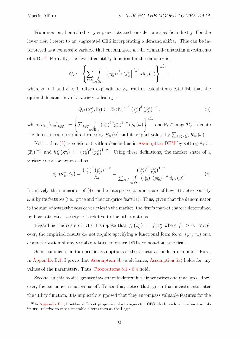
From now on, I omit industry superscripts and consider one specific industry. For the
lower tier, I resort to an augmented CES incorporating a demand shifter. This can be in-
terpreted as a composite variable that encompasses all the demand-enhancing investments
of a DL.31 Formally, the lower-tier utility function for the industry is,
Qi :=
∑
k∈C
∫
ω∈Ωki
[(zωki)
δσ−1 Qω
ki
]σ−1σ
dµi (ω)
σσ−1
,
where σ > 1 and δ < 1. Given expenditure Ei, routine calculations establish that the
optimal demand in i of a variety ω from j is
Qji
(xωji,Pi
):= Ei (Pi)σ−1 (zωji
)δ (pωji)−σ
, (3)
where Pi[(xki)k∈C
]:=
∑
k∈C∫
ω∈Ωki
(zωki)δ (pωki)
1−σ dµi (ω)
11−σ
and Pi ∈ rangePi. I denote
the domestic sales in i of a firm ω by Rii (ω) and its export values by∑
k∈C\iRik (ω).
Notice that (3) is consistent with a demand as in Assumption DEM by setting Ai :=
(Pi)1−σ and hωji(xωji)
:=(zωji)δ (
pωji)1−σ
. Using these definitions, the market share of a
variety ω can be expressed as
sji(xωji,Ai
)=
(zωji)δ (
pωji)1−σ
Ai
=
(zωji)δ (
pωji)1−σ
∑k∈C
∫ω∈Ωki
(zωki)δ (pωki)
1−σ dµi (ω). (4)
Intuitively, the numerator of (4) can be interpreted as a measure of how attractive variety
ω is by its features (i.e., price and the non-price feature). Thus, given that the denominator
is the sum of attractiveness of varieties in the market, the firm’s market share is determined
by how attractive variety ω is relative to the other options.
Regarding the costs of DLs, I suppose that fz(zωij)
:= f zzωij where f z > 0. More-
over, the empirical results do not require specifying a functional form for cji (ϕω, τji) or a
characterization of any variable related to either DNLs or non-domestic firms.
Some comments on the specific assumptions of the structural model are in order. First,
in Appendix B.3, I prove that Assumption 5b (and, hence, Assumption 5a) holds for any
values of the parameters. Thus, Propositions 5.1 - 5.4 hold.
Second, in this model, greater investments determine higher prices and markups. How-
ever, the consumer is not worse off. To see this, notice that, given that investments enter
the utility function, it is implicitly supposed that they encompass valuable features for the
31In Appendix B.1, I outline different properties of an augmented CES which made me incline towardsits use, relative to other tractable alternatives as the Logit.
24

Martın Alfaro 6 TAKING THE MODEL TO THE DATA
consumer. Also, with an augmented CES, the aggregate is a single sufficient statistic for
industry welfare. Therefore, since the aggregate’s value is the same under the simultane-
ous and sequential equilibrium, welfare measured at the industry level is the same in both
scenarios. In addition, the reallocation of market shares towards DLs in the sequential
scenario increases aggregate profits. If they are passed back to the consumer, there would
be greater consumption of the homogeneous good and, so, the consumer would be better
off. For more on welfare, see Appendix E.6.
6.2 Counterfactual and Outcomes
After solving the model under each scenario, the optimal solutions of prices and invest-
ments can be expressed in terms of market shares.32 This allows me to present the effect
of overinvestment on each industry through the following outcomes. First, given market
shares ssimii (ω) and sseq
ii (ω) for a firm ω, strategic gains are expressed through differences
in the domestic market share under each scenario. Moreover, given ssimii (ω) and industry
expenditures Ei, the revenues on the domestic market in the simultaneous case can be
recovered. Thus, with the information on domestic sales in each scenario along with the
export value∑
k∈C\iRik (ω) (which does not vary between scenarios), I can measure the
domestic intensity of each firm for both scenarios.
While sseqii (ω), Ei, and
∑k∈C\iRik (ω) are obtained from the data, it is necessary to
recover ssimii (ω). I outline how to obtain ssim
ii (ω), given (σ, δ) and sseqii (ω). The approach
exploits that market shares are determined structurally through (4), and that A∗i is the
same in the sequential and simultaneous cases. Expressing market shares in relative terms,
I obtainsseqii (ω)
ssimii (ω)
=[pωii (s
seqii (ω))]1−σ [zseq
ii (sseqii (ω))]δ
[pωii (ssimii (ω))]
1−σ[zsimii (ssim
ii (ω))]δ, (5)
where prices and investments correspond to the optimal solutions. Once these solutions are
incorporated into (4), ssimii (ω) is retrieved by knowledge of (σ, δ) and sseq
ii (ω).33 Intuitively,
ssimii (ω) is recovered by using how price and investment decisions vary structurally between
the scenarios, along with the impact on market shares that these changes entail.
32Specifically, they are given by pωii (sωii) = σσ−1
(1 + 1
σsωii
1−sωii
)cii (ϕω), zsim
ii (sωii) :=δsωii(1−s
ωii)
fzε(sωii), and
zseqii (sωii) :=
δsωii(1−sωii)
fzε(sωii)
(σ
σ−sωiiε(sωii)
).
33In Appendix B.4, I show that, given (σ, δ) and sseqii (ω), there exists a solution to (5) in terms of
ssimii (ω) and this is unique.
25

Martın Alfaro 7 EMPIRICAL ANALYSIS
Some remarks are in order. First, although market shares in (4) depend on c (ϕω) and
f z, their values cancel out in (5). The reason is that the marginal costs of producing and
investing do not change between scenarios. Second, (5) dictates that gains in market shares
can be estimated without knowing which firms the shares are reallocated from. While this
information affects the home-bias impact at the aggregate level, an upper bound of this is
still obtained by the total concentration increase accrued by DLs.
7 Empirical Analysis
For the empirics, I draw on information from Denmark provided by Statistics Denmark.
The datasets used are part of the country’s sources for official statistics. Several features
of the data make it appropriate for conducting the analysis. First, the information on
domestic firms’ sales and imports are disaggregated at the 8-digit product level, allowing
me to allocate each product to a properly-defined market. In addition, the information
of imports encompasses both manufacturing and non-manufacturing firms, thus providing
me with an accurate measure of import competition for each industry.
I start by describing the information included in the datasets. After this, I proceed
to construct the data analogs of the model concepts. Finally, I perform the quantitative
analysis. Alternative specifications that check the robustness of the results are included
in Appendix F.
7.1 Data Description
I make use of two datasets. One provides information about the production of man-
ufacturing firms. The other contains international transactions by both manufacturing
and non-manufacturing firms. Both datasets have information reported at the year-firm-
product level and can be easily merged through a unique firm identifier. I take 2005 as
the baseline year.34
The first dataset contains information about physical production in manufacturing
industries and constitutes the source for Danish Prodcom statistics. Any unit with at
least ten employees that lists manufacturing as its main activity is included. Overall, at
least 90% of the total production value in each NACE (revision 1.1) 4-digit industry is
34In Appendix F.1, I recalculate the results for all years between 2001 and 2007 and show that theaverage results are similar.
26

Martın Alfaro 7 EMPIRICAL ANALYSIS
covered.35 Products are defined in terms of the Combined Nomenclature at the 8-digit level
(hereafter, CN8), with information on values and quantities at the firm-product level.36
The second dataset is collected by Danish customs and reports imports (CIF values)
and exports (FOB values) at the CN8 firm-product level. It covers firms belonging to the
production dataset and also non-manufacturing firms. Overall, the trade flows recorded for
EU countries are 95% for imports and 97% for exports, while the universe of transactions
is covered for non-EU countries.
7.2 Definitions and Dataset
With the aim of defining market shares, it is necessary to establish the bounds of each
market, how sales are calculated, and some criteria to identify domestic firms and the
imports that compete with domestic products in the industry.
Regarding the definition of a market, I assemble the firm-product information at the
CN8 level such that it is defined as all the goods belonging to the same 4-digit NACE
industry. I keep referring to a sector as a 2-digit NACE industry. Moreover, I classify a
firm as domestic when it reports positive production in Denmark. The definition is applied
on an industry-by-industry basis and, so, some firms could be considered domestic in one
industry but not in another.
Market shares are defined relative to total sales value in the market. This comprises
sales by domestic firms and imports. Regarding the former, I take as a baseline case the
total turnover reported in the dataset of production.37 Results with alternative definitions
are presented in Appendix F.2.38 Moreover, I consider two types of imports as foreign
competition in an industry. The first type includes imports made by firms that do not
35NACE is the standard industry classification used in the EU. It is similar to the NAICS system forNorth American countries, or the older SIC used in the USA.
36The Combined Nomenclature is the nomenclature used by EU countries to report trade data. Theirfirst six digits coincide with the Harmonized System (HS) nomenclature.
37Since firms report their total value of production without a breakdown between domestic sales andexports, I compute the former as the difference between their total production value and its exports.
38Total turnover is not defined as production on the physical territory of Denmark. Instead, it is bythe economic ownership of goods sold and produced by Danish firms. Specifically, it includes sales ofown goods (either produced, processed or assembled by the firm), goods produced by a subcontractorestablished abroad (if the firm owns the inputs of the subcontracted firm), and resales of goods boughtfrom other domestic firms and sold with any processing. Essentially, it excludes sales of goods importedwhich are produced by foreign firms not owned by the Danish firm. Taking total production as the baselinesales is a conservative assumption to not either double count some of the imports, mistakenly considerexpenditure on inputs as outputs, or overestimate the market share of some firms which mainly act asretailers selling several brands. In Appendix F.2, I consider different definitions of firm imports as partof the total supply and show that results are essentially the same.
27

Martın Alfaro 7 EMPIRICAL ANALYSIS
engage in any production activity in Denmark. For instance, they comprise imports made
by retailers that are competing directly with sales by domestic firms. The second type
includes imports made by domestic firms not producing in that industry. These imports
represent foreign competition since they are inputs that the firm could have bought from
a domestic firm. Figure 5 illustrates the classification.
Figure 5. Classification by Industry into Domestic Firms and Import Competition
INDUSTRY 1
INDUSTRY 2
Firm 1
Firm 2
Domestic Production
Domestic Production
Retailer
ImportedGoods
ImportedInputs
ImportCompetitionof Industry 1
Note: The classification of a firm as domestic or part of the import competition is conducted at the industry level. Thus,a firm can be domestic in one industry but represent import competition in another. In the figure, I illustrate this byconsidering two firms. Firm 1 and 2 are domestic in industries 1 and 2, respectively, since each sells a good that belongsto that industry. In industry 1, the import competition encompasses imports of industry 1’s goods by non-manufacturingfirms (e.g., retailers) and manufacturing firms that do not produce goods belonging to industry 1 (e.g., Firm 2).
I consider a Danish firm-industry as a DL if it has a domestic market share greater than
3%. Remarkably, given that the structural model determines that a DL with negligible
market shares behaves as a DNL, the cutoff only affects the presentation of average results,
but not the impact at the industry level.
Consistent with the theoretical model, I only consider industries which include a subset
of firms having negligible market shares, and drop those that exhibit no import competi-
tion.39 After this, I end up with 107 industries out of a total of 203. The sample of indus-
tries covers around 80% of the total value of the manufacturing. At the firm-industry level
and in terms of Danish firms, it encompasses 331 DLs and 5,350 DNLs. Furthermore, since
92 industries have at least one DL, it reveals that the standard monopolistic-competition
market structure with negligible firms is valid for only 15 out of 107 industries.
7.3 Determination of Parameters
To obtain the counterfactual in Section 6.2, I have assumed that σ and δ are given. Now I
proceed to their determination. For σ, I make use of the estimates provided by Soderbery
(2015). His approach is based on Broda and Weinstein (2006) and improves upon it to
39The procedure, as well as additional results, are presented in Appendix C.1.
28
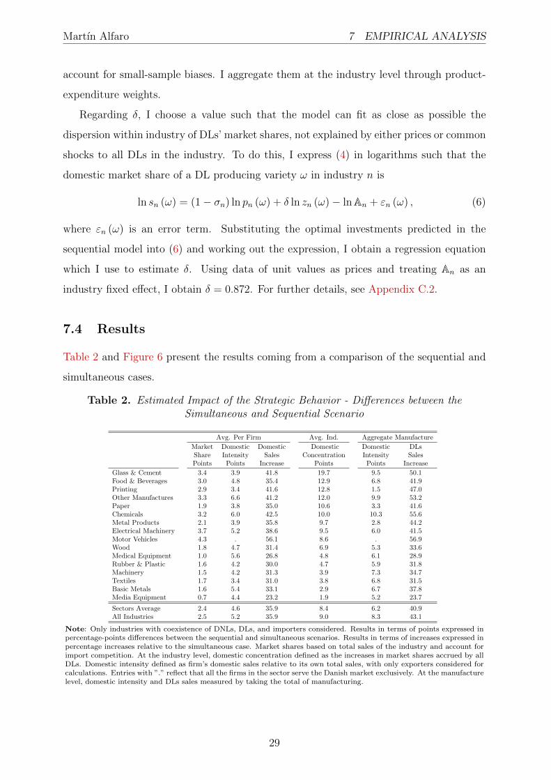
Martın Alfaro 7 EMPIRICAL ANALYSIS
account for small-sample biases. I aggregate them at the industry level through product-
expenditure weights.
Regarding δ, I choose a value such that the model can fit as close as possible the
dispersion within industry of DLs’ market shares, not explained by either prices or common
shocks to all DLs in the industry. To do this, I express (4) in logarithms such that the
domestic market share of a DL producing variety ω in industry n is
ln sn (ω) = (1− σn) ln pn (ω) + δ ln zn (ω)− lnAn + εn (ω) , (6)
where εn (ω) is an error term. Substituting the optimal investments predicted in the
sequential model into (6) and working out the expression, I obtain a regression equation
which I use to estimate δ. Using data of unit values as prices and treating An as an
industry fixed effect, I obtain δ = 0.872. For further details, see Appendix C.2.
7.4 Results
Table 2 and Figure 6 present the results coming from a comparison of the sequential and
simultaneous cases.
Table 2. Estimated Impact of the Strategic Behavior - Differences between theSimultaneous and Sequential Scenario
Avg. Per Firm Avg. Ind. Aggregate Manufacture
Market Domestic Domestic Domestic Domestic DLsShare Intensity Sales Concentration Intensity SalesPoints Points Increase Points Points Increase
Glass & Cement 3.4 3.9 41.8 19.7 9.5 50.1Food & Beverages 3.0 4.8 35.4 12.9 6.8 41.9Printing 2.9 3.4 41.6 12.8 1.5 47.0Other Manufactures 3.3 6.6 41.2 12.0 9.9 53.2Paper 1.9 3.8 35.0 10.6 3.3 41.6Chemicals 3.2 6.0 42.5 10.0 10.3 55.6Metal Products 2.1 3.9 35.8 9.7 2.8 44.2Electrical Machinery 3.7 5.2 38.6 9.5 6.0 41.5Motor Vehicles 4.3 . 56.1 8.6 . 56.9Wood 1.8 4.7 31.4 6.9 5.3 33.6Medical Equipment 1.0 5.6 26.8 4.8 6.1 28.9Rubber & Plastic 1.6 4.2 30.0 4.7 5.9 31.8Machinery 1.5 4.2 31.3 3.9 7.3 34.7Textiles 1.7 3.4 31.0 3.8 6.8 31.5Basic Metals 1.6 5.4 33.1 2.9 6.7 37.8Media Equipment 0.7 4.4 23.2 1.9 5.2 23.7
Sectors Average 2.4 4.6 35.9 8.4 6.2 40.9All Industries 2.5 5.2 35.9 9.0 8.3 43.1
Note: Only industries with coexistence of DNLs, DLs, and importers considered. Results in terms of points expressed inpercentage-points differences between the sequential and simultaneous scenarios. Results in terms of increases expressed inpercentage increases relative to the simultaneous case. Market shares based on total sales of the industry and account forimport competition. At the industry level, domestic concentration defined as the increases in market shares accrued by allDLs. Domestic intensity defined as firm’s domestic sales relative to its own total sales, with only exporters considered forcalculations. Entries with ”.” reflect that all the firms in the sector serve the Danish market exclusively. At the manufacturelevel, domestic intensity and DLs sales measured by taking the total of manufacturing.
29

Martın Alfaro 7 EMPIRICAL ANALYSIS
Figure 6. Sequential vs. Simultaneous Scenarios(a) Domestic Concentration - Levels
56
36
44
31
39
26
32
20
35
25
30
20
33
23
31
2124
15
25
18
22
17 18
1315
1114
10 118
108
Gla
ss &
Cem
ent
Food
−Bev
erag
esPr
intin
g
Oth
er M
anuf
actu
res
Pape
rC
hem
ical
sM
etal
Pro
duct
s
Elec
trica
l Mac
hine
ryM
otor
Veh
icle
sW
ood
Med
ical
Equ
ipm
ent
Rub
ber &
Pla
stic
Mac
hine
ryTe
xtile
sBa
sic
Met
als
Med
ia E
quip
men
t
Sequential Case Simultaneous Case
(b) Domestic Concentration - Points Increase byIndustry
010
2030
40P
erce
ntag
e P
oint
sG
lass
& C
emen
t
Food
−Bev
erag
esPr
intin
g
Oth
er M
anuf
actu
res
Pape
rC
hem
ical
sM
etal
Pro
duct
s
Elec
trica
l Mac
hine
ryM
otor
Veh
icle
sW
ood
Med
ical
Equ
ipm
ent
Rub
ber &
Pla
stic
Mac
hine
ryTe
xtile
sBa
sic
Met
als
Med
ia E
quip
men
t
Industry’s Gains Sector’s Average Gains
(c) Firm’s Domestic Market Share - PointsIncrease per Firm
05
1015
20P
erce
ntag
e P
oint
sG
lass
& C
emen
t
Food
−Bev
erag
esPr
intin
g
Oth
er M
anuf
actu
res
Pape
rC
hem
ical
sM
etal
Pro
duct
s
Elec
trica
l Mac
hine
ryM
otor
Veh
icle
sW
ood
Med
ical
Equ
ipm
ent
Rub
ber &
Pla
stic
Mac
hine
ryTe
xtile
sBa
sic
Met
als
Med
ia E
quip
men
t
Firm’s Gains Sector’s Average Gains
(d) Firm’s Domestic Intensity - Points Increaseper Firm
05
1015
20P
erce
ntag
e P
oint
sG
lass
& C
emen
t
Food
−Bev
erag
esPr
intin
g
Oth
er M
anuf
actu
res
Pape
rC
hem
ical
sM
etal
Pro
duct
s
Elec
trica
l Mac
hine
ryM
otor
Veh
icle
sW
ood
Med
ical
Equ
ipm
ent
Rub
ber &
Pla
stic
Mac
hine
ryTe
xtile
sBa
sic
Met
als
Med
ia E
quip
men
t
Firm’s Gains Sector’s Average Gains
Note: Figure 6a expressed in market-share levels. In the rest of the figures, outcomes are percentage-points differencesbetween the sequential and simultaneous case. Figures with firm’s domestic intensity excludes firms that sell exclusivelyin the domestic market. Market shares measured in terms of total sales value of the industry and account for importcompetition.
The first conclusion is that there is pronounced heterogeneity in concentration out-
comes across sectors (Figure 6a) and industries (Figure 6b). Regarding firms, the market
shares of the top 3 DLs, which are respectively around 14%, 7%, and 6% in the sequential
scenario, would instead have been 9%, 5%, and 5% in the simultaneous scenario. Nonethe-
less, Figure 6c reveals that these gains can be substantially greater for some of the firms.
In terms of domestic intensity, the top DL has increases of around 4% and 6%, respectively,
depending on whether all firms or just exporters are considered. For the same cases, both
the second and third top DLs have increases of around 2% and 4%, on average. From
Figure 6d, it is clear that there is also pronounced heterogeneity in terms of domestic
intensity.
Arguably, the magnitude of estimates coming from structural models should be inter-
preted with caution, given the simplifications and assumptions made about unobservables.
On the other hand, the approach is a powerful tool for comparing the relative importance
of a mechanism across different groups of observations. Showing how outcomes differ by
30

Martın Alfaro 7 EMPIRICAL ANALYSIS
groups of industries is of relevance for this paper, given the stark differences in the results
obtained across them.
At a theoretical level, by Propositions 5.1 - 5.4, market-share gains and increases in
domestic intensity are always positive. Nevertheless, these results are silent about their
magnitudes. In the structural model, it can be shown that the strength of the effects dis-
play non-monotonicities in relation to the market shares and domestic intensity observed.
However, as demonstrated via simulations in Appendix B.5, for the range of values in the
data, the sign of the relations can be predicted. This is because, on average, firms have
market shares that are not disproportionately large, while home-bias is pronounced. Both
facts also determine that differences in σ have a small direct impact on the results. Thus,
the magnitude of concentration gains is mainly determined by the level of concentration
observed, while increases in domestic intensity are primarily determined by both market
shares and domestic intensity observed.
This provides me with some guidance for identifying the industries where the impact of
strategic investments should be more pronounced. First, regarding concentration, if DLs
accumulate a small market share, they will have a small influence on the aggregate condi-
tions of the market. Thus, they will obtain only a small strategic gain of market shares.
Additionally, in industries where firms, on average, sell almost exclusively in their home
market, domestic-intensity increases will be less affected by greater domestic revenues.
Based on this intuition, the correlation patterns in Stylized Fact 3 are informative. They
point out that lower values of σ are associated with greater concentration and lower do-
mestic intensity in industries with consumer goods, and lower concentration for producer
goods. Thus, I proceed to analyze the outcomes in terms of good substitutability.
Classifying industries in terms of low and high σ (relative to the whole manufacturing
sector), the results indicate that strategic gains arise in 65 and 27 industries, respec-
tively.40 As for the magnitude of outcomes in relation with σ, regressions that pool all
the observations suggest that there is no relation. However, this unmasks heterogeneity
across industries, with a pattern emerging once that I classify them according to their
40Similar results arise by breaking down industries into differentiated and homogeneous goods as inRauch (1999). This determines that 68 industries are differentiated and 24 homogeneous. Nonetheless,unlike σ, they do not constitute a good predictor of the level of concentration. In addition, the classificationby Rauch (1999) should be interpreted with some caution depending on the analysis carried out. As Brodaand Weinstein (2006) indicate, the classification, although correlated with σ, does not imply that when agood is labeled as homogeneous it is perceived as a perfect substitute. They provide tea as an example,which is considered as a homogeneous good by Rauch (1999), but it surely is perceived to be quitedifferentiated by consumers (the same remark applies to, for instance, beer).
31

Martın Alfaro 7 EMPIRICAL ANALYSIS
final user (i.e., producer vs consumer). To make the comparison meaningful, I discard
sectors where all the industries are classified exclusively as either comprising producer
or consumer goods.41 This determines that there are, respectively, 24 and 20 industries
with producer and consumer goods displaying strategic gains. The results are presented
in Table 3.
Table 3. Substitutability and Final Users (consumers vs producers)
Concentration Increase Domestic Intensity IncreaseBW-S σ σ constant BW-S σ σ constant
DLs Top 3 Non-Top 3 DLs Top 3 Non-Top 3(1) (2) (3) (4) (5) (6) (7) (8) (9) (10)
lnσ (consumers) -16.16** -14.79** -1.369 -12.66** -11.38* -1.283 -2.886** -2.861* -3.053*** -2.308*(7.405) (6.997) (1.192) (6.925) (6.039) (1.139) (1.150) (1.442) (1.099) (1.345)
lnσ (producers) 7.970** 5.581* 2.120 9.903** 7.726** 2.177 -1.113 0.041 -1.090 -1.024(3.615) (3.258) (1.515) (3.680) (3.089) (1.524) (1.084) (3.387) (1.365) (4.154)
Sector FE Yes Yes Yes Yes Yes Yes Yes YesSector-Rank FE Yes YesSample Unit Industry Industry Industry Industry Industry Industry Firm-Ind Exp-Ind Firm-Ind Exp-IndObservations 39 39 39 39 39 39 170 104 139 81R-squared 0.305 0.292 0.306 0.301 0.283 0.308 0.251 0.211 0.367 0.271
Note: Domestic Leaders (DLs) in an industry defined as Danish firms with a domestic market share greater than 3%. In-dustries with producer and consumer goods defined according to the BEC classification, with producer goods encompassingintermediate goods and capital. The variable BW-S σ corresponds to the elasticity of substitution from Soderbery (2015).Rank refers to the position in the market according to the domestic market share of the firm. Firm-Ind indicates thatthe observations are at the firm-industry level, while Exp-ind indicates that the sample is restricted to firms that export.All the results come from regressions of the type y = FEs + α lnσ + β × 1(user). By including all the interaction termsthrough the fixed effects FEs, the α estimated is identical to that obtained through a separate regression with the samplerestricted to one type of final user. Heteroskedastic-robust standard errors used.
The parameter estimates in Columns (1) to (3) indicate that a lower σ is associated
with greater gains of market shares for consumer goods. The opposite result is obtained
for producer goods, where greater increases in concentration are found in industries with
greater values of σ. Moreover, while this holds for the concentration by the top 3 DLs,
there are no statistically significant differences for the non-top DLs.
Since the outcomes are calculated using σ, and a greater σ determines a smaller impact
on the gains of market share, we may suspect that this is driving the results. This is
especially the case for consumer goods where the sign of the results are consistent with
an explanation along those lines. I provide evidence that this is not the case and, instead,
it responds to the pattern of concentration of consumer and producer goods implied by
Stylized Fact 3. To corroborate this, in Columns (4) to (6), I present estimates obtained
by assuming σ is constant across industries. The results are consistent with Columns (1)
to (3).
In addition, for consumer goods, Columns (7) and (8) establish that the domestic-
intensity increases are more pronounced for industries with lower values of σ. This is
41I have also discarded the machinery sector since it has 11 industries with producer goods and justone with consumer goods.
32

Martın Alfaro 8 CONCLUSIONS
irrespective of whether all DLs or just those that export are considered. On the contrary,
there seems to be no relation between σ and domestic-intensity increases for the case of
producer goods. In Columns (9) and (10), to isolate the role of the domestic-intensity
distribution, I replicate the results by keeping σ constant across industries and control-
ling for the rank position by market share. This corroborates that the distribution of
domestic intensity indicated in Stylized Fact 3 is important in the determination of these
outcomes. Moreover, the results also indicate that the same qualitative outcomes are
obtained irrespective of whether the sample is restricted to exporters.42
8 Conclusions
In this paper, I studied a mechanism in which domestic leaders engage in strategic behavior
to preempt entry and gain a better position in their home market. In order to analyze the
phenomenon, I built up a framework which tractably incorporates strategic interactions
and an endogenous number of heterogeneous firms making multiple choices. Given the
flexibility of the setup, I was able to conduct the study at both the theoretical and empirical
level.
The model combines the technical advantages of two different approaches. First, I
based my approach on an empirical fact that I identified in my data, where in a typical
industry there is coexistence of leaders and firms with trivial market shares. Thus, I
exploited the parsimonious approach of Melitz (2003) to model the behavior of negligible
firms and account for extensive-margin adjustments. Second, I resorted to the tools of
Aggregative Games to tractably incorporate the existence of heterogeneous firms behaving
strategically and deciding on multidimensional strategies. This turns a potentially complex
multidimensional problem into a unidimensional one.
At the theoretical, I established that, relative to a non-strategic benchmark, domestic
leaders overinvest on demand-enhancing instruments at their home market, resulting in a
crowding out of rival firms and, in particular, of importers. This strategy causes a real-
location of market share towards domestic leaders which generates greater concentration
and home-bias patterns at both the firm and industry level. I showed that the outcomes
are robust to the type of competition at the market stage (prices or quantities), the effect
of investments on prices (increases or decreases), and even the nature of investments (i.e.,
42In addition, it can be shown that the results hold by including market shares as a control variable.
33

Martın Alfaro 8 CONCLUSIONS
cost-reducing or demand-enhancing).
Turning the theoretical model into a structural one, I conducted an empirical study
of the mechanism by making use of disaggregated Danish manufacturing data. I showed
that, in industries with consumer goods, a lower substitutability is associated with greater
increases of concentration and domestic intensity. On the contrary, for producer goods,
industries with lower substitutability have lower concentration gains and display statisti-
cally insignificant differences in terms of domestic intensity. I provided evidence that the
main determinants of these results are the distributions of market shares and domestic
intensity in relation to substitutability.
34

Martın Alfaro REFERENCES
ReferencesAcemoglu, D. and M. K. Jensen (2013). Aggregate Comparative Statics. Games and Economic Behav-
ior 81, 27–49. 1, 4.2
Amiti, M. and A. K. Khandelwal (2013). Import Competition and Quality Upgrading. The Review ofEconomics and Statistics 95 (2), 476–490. C.2
Anderson, S., N. Erkal, and D. Piccinin (2016). Aggregative oligopoly games with entry. 49
Arkolakis, C., A. Costinot, D. Donaldson, and A. Rodrıguez-Clare (2019). The elusive pro-competitiveeffects of trade. The Review of Economic Studies 86 (1), 46–80. 26, E.1
Armington, P. (1969). A theory of demand for products distinguished by place of production. StaffPapers 16 (1), 159–178. 13
Atkeson, A. and A. Burstein (2008). Pricing-to-Market, Trade Costs, and International Relative Prices.American Economic Review 98 (5), 1998–2031. 10
Autor, D., D. Dorn, L. F. Katz, C. Patterson, and J. Van Reenen (2017). The fall of the labor share andthe rise of superstar firms. Working Paper 23396, National Bureau of Economic Research. 1, 12
Axtell, R. L. (2001). Zipf Distribution of US Firm Sizes. Science 293 (5536), 1818–1820. 18
Baumol, W., J. Panzar, and R. Willig (1982). Contestable Markets and the Theory of Industry Structure.Harcourt Brace Jovanovich. 1
Bell, D. E., R. L. Keeney, and J. D. Little (1975). A market share theorem. Journal of MarketingResearch 12 (2), 136–141. B.1
Bernard, A., J. Jensen, S. Redding, and P. Schott (2012). The Empirics of Firm Heterogeneity andInternational Trade. Annual Review of Economics 4 (1), 283–313. 1, 19
Berry, S., M. Gaynor, and F. Scott Morton (2019, August). Do increasing markups matter? lessons fromempirical industrial organization. Journal of Economic Perspectives 33 (3), 44–68. 1
Bertoletti, P. and F. Etro (2015). Monopolistic Competition When Income Matters. The EconomicJournal . 26, E.1
Boulding, W. and M. Christen (2009). Pioneering plus a broad product line strategy: Higher profits ordeeper losses? Management Science 55 (6), 958–967. 4
Broda, C. and D. E. Weinstein (2006). Globalization and the Gains From Variety. The Quarterly Journalof Economics 121 (2), 541–585. 9, 3, 7.3, 40
Caron, J., T. Fally, and J. R. Markusen (2014). International trade puzzles: A solution linking productionand preferences. The Quarterly Journal of Economics 129 (3), 1501–1552. 13
Chaney, T. (2014). The network structure of international trade. American Economic Review 104 (11),3600–3634. 1, 13
Cosar, A. K., P. L. Grieco, S. Li, and F. Tintelnot (2018). What drives home market advantage? Journalof international economics 110, 135–150. 17
De Loecker, J. and J. Eeckhout (2017). The rise of market power and the macroeconomic implications.Working Paper 23687, National Bureau of Economic Research. 12
De Loecker, J. and J. Eeckhout (2018). Global market power. Technical report, National Bureau ofEconomic Research. 12
Dunning, J. H. (1977). Trade, location of economic activity and the MNE: A search for an eclecticapproach. In The international allocation of economic activity, pp. 395–418. Springer. 2
35

Martın Alfaro REFERENCES
Eaton, J., S. S. Kortum, and S. Sotelo (2012). International Trade: Linking Micro and Macro. WorkingPaper 17864, National Bureau of Economic Research. 10, 11
Edmond, C., V. Midrigan, and D. Y. Xu (2015). Competition, Markups, and the Gains from InternationalTrade. American Economic Review 105 (10), 3183–3221. 10
Etro, F. (2006). Aggressive Leaders. The RAND Journal of Economics 37 (1), 146–154. 3
Fudenberg, D. and J. Tirole (1991). Game Theory. MIT Press. 1, 5
Fujiwara, Y., C. Di Guilmi, H. Aoyama, M. Gallegati, and W. Souma (2004). Do Pareto–Zipf andGibrat laws hold true? An analysis with European firms. Physica A: Statistical Mechanics and itsApplications 335 (1-2), 197–216. 18
Gaubert, C. and O. Itskhoki (2018). Granular comparative advantage. 10, 11
Gutierrez, G. and T. Philippon (2017). Declining competition and investment in the u.s. Working Paper23583, National Bureau of Economic Research. 12
Hillberry, R. and D. Hummels (2002). Explaining home bias in consumption: The role of intermediateinput trade. Technical report, National Bureau of Economic Research. 13
Hottman, C., S. J. Redding, and D. E. Weinstein (2016). Quantifying the Sources of Firm Heterogeneity.The Quarterly Journal of Economics. 18
Hymer, S. (1960). On multinational corporations and foreign direct investment. The theory of transna-tional corporations. London: Routledge for the United Nations. 2
Isaacson, W. (2011). Steve Jobs: A Biography. Thorndike Press. 1
Jensen, M. K. (2018). Aggregative games. In Handbook of Game Theory and Industrial Organization,Volume I, Chapters, Chapter 4, pp. 66–92. Edward Elgar Publishing. 25
Mayer, T. and G. Ottaviano (2008). The Happy Few: The Internationalisation of European Firms.Intereconomics- Review of European Economic Policy 43 (3), 135–148. 19, 3
McCallum, J. (1995). National Borders Matter: Canada-U.S. Regional Trade Patterns. American Eco-nomic Review 85 (3), 615–623. 1
McFadden, D. (1973). Conditional Logit Analysis of Qualitative Choice. Frontiers in Econometrics.Academic Press. 26, E.1
Melitz, M. J. (2003). The Impact of Trade on Intra-industry Reallocations and Aggregate IndustryProductivity. Econometrica 71 (6), 1695–1725. 1, 4.1, 4.2, 8, E.2
Milgrom, P. and C. Shannon (1994). Monotone comparative statics. Econometrica 62 (1), 157–180. 5
Nocke, V. and N. Schutz (2018). Multiproduct-firm oligopoly: An aggregative games approach. Econo-metrica 86 (2), 523–557. 26, E.1, 49, 50
Obstfeld, M. and K. Rogoff (2001). The Six Major Puzzles in International Macroeconomics: Is There aCommon Cause? In NBER Macroeconomics Annual 2000, Volume 15, pp. 339–412. MIT press. 1
Parenti, M. (2018). Large and small firms in a global market: David vs. Goliath. Journal of InternationalEconomics 110, 103–118. 6
Paton, D. (2008). Advertising as an Entry Deterrent: Evidence from UK firms. International Journal ofthe Economics of Business 15 (1), 63–83. 4
Porter, M. (1998). Competitive Advantage: Creating and Sustaining Superior Performance. Free Press. 2
Porter, M. E. (1980). Competitive Strategy: Techniques for Analyzing Industries and Competitors.Competitive Strategy 1 (6), 396. 14
36
Martın Alfaro REFERENCES
Porter, M. E. (2011). Competitive Advantage of Nations: Creating and Sustaining Superior Performance.Simon and Schuster. 14
Rauch, J. E. (1999). Networks versus markets in international trade. Journal of International Eco-nomics 48 (1), 7 – 35. 40
Schelling, T. (1960). The Strategy of Conflict. Harvard University Press. 2, 15
Shimomura, K.-I. and J.-F. Thisse (2012). Competition among the big and the small. The RAND Journalof Economics 43 (2), 329–347. 6
Soderbery, A. (2015). Estimating import supply and demand elasticities: Analysis and implications.Journal of International Economics 96 (1), 1 – 17. 9, 3, 1, 7.3, 3, C.2
Sutton, J. (1991). Sunk Costs and Market Structure: Price Competition, Advertising, and the Evolutionof Concentration. MIT press. 1, 6
Sutton, J. (1996). Game theoretical models of market structure. Mimeo. 7
Sutton, J. (1998). Technology and Market Structure: Theory and History. Theory and History. MIT Press.1
Takayama, A. (1993). Analytical Methods in Economics. University of Michigan Press. 27
Tirole, J. (1988). The Theory of Industrial Organization. Cambridge, Mass. 2
Trefler, D. (1995). The Case of the Missing Trade and Other Mysteries. American Economic Review 85 (5),1029–1046. 1
Vives, X. (2001). Oligopoly Pricing: Old Ideas and New Tools (1 ed.), Volume 1. The MIT Press. E.1
Yi, K.-M. (2010). Can multistage production explain the home bias in trade? American EconomicReview 100 (1), 364–93. 13
37

Martın Alfaro A DERIVATIONS AND PROOFS
Online Appendix - not for
publication
A Derivations and Proofs
In this appendix, I provide derivations of some results included in Section 5 regarding the
sequential scenario. In particular, I present a formal justification for the fact that the
aggregate is the same in the simultaneous and sequential scenarios. After this, I present
proofs for Propositions 5.1 - 5.4.
A.1 Derivations of the Sequential Scenario
Denote by zii := (zωii)ω∈ΩBiiand zdom := (zii)i∈C the vector of domestic investments by DLs
from i and by DLs around the world, respectively. As argued in the main part of the paper,
the simultaneous game with a given zdom defines a class of subgames for the sequential
scenario. Furthermore, since markets are segmented, zdom can only affect market i through
zii. Using these facts, next I characterize the solution of this subgame in i ∈ C for a given
zii.
Regarding optimal choices, notice that, conditional on Ai, the profits of both DNLs
and non-domestic firms in i do not depend on zii. Thus, the optimal decisions of these
firms are the same as in the simultaneous scenario: their prices, investments, and survival
productivity cutoffs are still characterized by (PRICE), (z-SIM), and (ZCP), respectively.
On the other hand, zii affects the pricing of DLs from i. The optimal price of a firm ω is
still characterized by (PRICE) but it determines a solution pωii (zωii,Ai, ϕω).
With the optimal choices determined and conditional on a given zii, the equilibrium
of the subgame can be obtained as in the simultaneous scenario. To do this, let’s define
the aggregate backward-response function of country i:
Γi(Ai,ME , zii
):=Hi
∑
k∈CMEk
∫ ϕk
ϕki(Ai)hSki[xSki (Ai, ϕ)
]dGSk (ϕ) +
∑
j∈C\i
∫
ω∈ΩBji
hωji[xωji (Ai, ϕω)
]dµi (ω) +
∑
ω∈ΩBii
hωii [pωii (zωii,Ai, ϕω) , zωii]
. (7)
A-1

Martın Alfaro A DERIVATIONS AND PROOFS
Thus, the Nash equilibrium in i requires that Ai constitutes a fixed point of (7). Formally,
Γ(Ai,M
E, zii)
= Ai. (NE-seq)
Finally, since zii does not directly affect the profits of DNLs conditional on Ai, the free-
entry condition for each i remains identical as in the simultaneous case and given by
(FE).
From all this, we conclude that an equilibrium of the subgame for a given zii is obtained
through values MEseq :=
(ME∗
i (zii))i∈C and (Aseq
i (zii))i∈C such that (FE) and (NE-seq) for
each i ∈ C hold. Once that these values are pinned down, the optimal strategies can also
be obtained for a given zdom.
Next, I establish some properties of the subgame equilibrium with the goal of showing
that zii cannot affect the equilibrium aggregates but only the mass of DNLs. To keep
track of these features, I state them as properties. They follow by simple inspection of the
equilibrium conditions.
Subgame Equilibrium Property P1. Conditional on Ai, the optimal choices made by
DNLs and foreign firms in i are independent of ME, zdom and (Aj)j 6=i.
It is worth remarking that Property P1 does not imply that optimal choices are inde-
pendent of any variable chosen by a rival firm. Rather, it states that, if any variable has
an effect on them, it has to be indirectly and through Ai.
Property P1 characterizes the decisions in i for all firms except DLs from i. For those,
the following property holds.
Subgame Equilibrium Property P2. The optimal price at home of a DL ω from i
is completely determined by Ai and zωii. This implies that, conditional on Ai and zωii, its
domestic pricing decision is independent of ME, (Aj)j 6=i, (zjj)j 6=i and(zω′
ii
)ω′ 6=ω.
Property P2 establishes that, regarding information of the industry conditions, the
investment decisions by DLs are made by taking Ai as a single sufficient statistic. Its
composition is irrelevant. Thus, conditional on Ai, the values of(zω′
ii
)ω′ 6=ω or ME do not
convey any valuable information to the firm. Consequently, by establishing how (Aseqi )i∈C
is identified, the investment decisions by DLs are also characterized.
To inquire upon how (Aseqi )i∈C is determined, by inspection of the equilibrium conditions
(FE) and (NE-seq), it can be noticed that ME does not influence directly the expected
A-2

Martın Alfaro A DERIVATIONS AND PROOFS
profits of any DNL and, hence, (FE). Consequently, the system (FE) for each i ∈ Ccompletely pins down the equilibrium aggregates. Thus, the following property holds.
Subgame Equilibrium Property P3. The system (FE) for each i ∈ C pins down the
equilibrium value (Aseqi )i∈C independently of ME. Furthermore, given (Aseq
i )i∈C, MEseq is
determined by the system of equations (NE-seq) for each i ∈ C.
Property P3 has a simple interpretation. In equilibrium, the free-entry conditions of
DNLs around the world completely determine the equilibrium aggregates. Given these
values, the masses of DNLs adjust such that there is no excess of supply in equilibrium,
making (NE-seq) hold in each country. Finally, all the properties stated lead to the
following conclusion.
Subgame Equilibrium Property P4. zdom cannot affect (Aseqi )i∈C. It only affects ME
seq.
Property P4 provides a formal justification for the claim stated in the main part of
the paper: the simultaneous and sequential games share the same equilibrium aggregates
(A∗i )i∈C. Variations in zii only affect the mass of DNLs.
A.2 Proofs of Section 5.3
Proof of Proposition 5.1. We know that, under both scenarios, the same (A∗k)k∈C holds
and DLs choose a level of investment from the same choice set Z. Thus, if in the sequential
game DLs chose the same level of investments as in the simultaneous case, they would
achieve the same profits. Hence, by a revealed-preference argument, πseqi (ω) ≥ πsim
i (ω).
Furthermore, by the strictly-pseudo concavity and Assumption 5a, it can be shown that
the level of investments in each scenario differ (this is shown formally in the proof of
Proposition 5.2). Thus, by the strictly-pseudo concavity, this fact implies that πseqi (ω) >
πsimi (ω).
For the subsequent proofs, I make use of the following lemma.
Lemma A.1. For a given A∗i , conditiondAi[pωii(zωii;A∗i ,ϕω),zωii,A∗i ]
dzωii> 0 holds if and only if
∂ ln pωii(zωii;A∗i ,ϕω)∂ ln zωii
<εz,mcii (zωii;A∗i ,ϕω)−εzii(zωii;A∗i ,ϕω)εp,mcii (zωii;A∗i ,ϕω)−εpii(zωii;A∗i ,ϕω)
.
Proof of Lemma A.1. The statement can be equivalently rephrased as sgn
dAi[·]dzωii
=
sgn
εz,mcii [·]−εzii[·]εp,mcii [·]−εpii[·]
− ∂ ln pωii(zωii;A∗i ,ϕω)∂ ln zωii
. By definition,
εz,mcii [·]−εzii[·]εp,mcii [·]−εpii[·]
=− ∂ lnQωii[·]
∂ ln Ai∂ lnAi[·]∂ ln zω
ii∂ lnQω
ii[·]
∂ lnAi∂ lnAi[·]∂ ln pω
ii
or, what
A-3

Martın Alfaro A DERIVATIONS AND PROOFS
is same,εz,mcii [·]−εzii[·]εp,mcii [·]−εpii[·]
=− ∂ lnAi[·]
∂ ln zωii
∂ lnAi[·]∂ ln pω
ii
. Moreover, d lnAi[·]d ln zωii
=∂ lnAj [·]∂ ln zωii
+∂ lnAj [·]∂ ln pωii
∂ ln pωii(·)∂ ln zωii
, so that
d lnAj [·]d ln zωii
> 0 iff∂ lnAj [·]∂ ln zωii
+∂ lnAj [·]∂ ln pωii
∂ ln pωii(·)∂ ln zωii
> 0, which holds iff∂ ln pωii(·)∂ ln zωii
<− ∂ lnAi[·]
∂ ln zωii
∂ lnAi[·]∂ ln pω
ii
.
Proof of Proposition 5.2. Consider the decisions in the home market by a DL ω from
i with productivity ϕω. The marginal profits of domestic investments in the simultaneous
and sequential case are given, respectively, by
γsimω (xωii,Ai;ϕω) :=
∂πωii (xωii,Ai;ϕω)
∂zωii+∂πωii (xωii,Ai;ϕω)
∂Ai
∂Ai[(xki)k∈C
]
∂zωii(8a)
γseqω (xωii,Ai;ϕω) :=
∂πωii (xωii,Ai;ϕω)
∂zωii+∂πωii (xωii,Ai;ϕω)
∂pωii
∂pωii (zωii,Ai, ϕω)
∂zii. (8b)
Independently of whether we consider the simultaneous or sequential case, optimal prices
are characterized by (PRICE). This implies that∂πωii(·)∂pωii
= −∂πωii(·)∂Ai
∂Ai[·]∂pωii
and, so, we can
reexpress (8b) as
γseqω (xωii,Ai;ϕω) :=
∂πωii (xωii,Ai;ϕω)
∂zωii− ∂πωii (xωii,Ai;ϕω)
∂Ai
∂Ai[(xki)k∈C
]
∂pωii
∂pωii (zωii,Ai, ϕω)
∂zωii.
Let A∗i be the equilibrium aggregate under the simultaneous and sequential case, and
zsimii (ω) the optimal investments of the firm ω in the simultaneous scenario. Also, denote
the domestic prices in the simultaneous scenario by psimii (ω) := pωii
[zsimii (ω) ,A∗i , ϕω
].
Evaluating (8a) at the simultaneous equilibrium, we get γsimω
[xsimii (ω) ,A∗i ;ϕω
]= 0.
Given the pseudo-concavity of the profits function, if we show that γseqω
[xsimii (ω) ,A∗i ;ϕω
]>
0, then the result follows. Defining
∆simω :=: ∆ω
[xsimii (ω) ,A∗i ;ϕω
]:= γseq
ω
[xsimii (ω) ,A∗i ;ϕω
]− γsim
ω
[xsimii (ω) ,A∗i ;ϕω
],
we need to show that ∆simω > 0. Then,
∆simω = −∂π
ωii (·)∂Ai
[∂Ai (A∗i )∂pωii
∂pωii[zsimii (ω) ,A∗i , ϕω
]
∂zωii+∂Ai (A∗i )∂zωii
],
where∂Ai(A∗i )∂zωii
is shorthand notation for the fact that I am evaluating the derivative at A∗i .
Given∂πωii(·)∂Ai < 0, Assumption 5a, and Lemma A.1, the term in brackets is positive and,
so, the result follows.43
Proof of Proposition 5.3. For a given A∗i , the revenues of a DL ω as a function of its
investments are Rωii (z
ωii;A∗i , ϕω) := Rω
ii [pωii (z
ωii;A∗i , ϕω) , zωii,A∗i ] which, in turn, are given by
the product Qωii [p
ωii (z
ωii;A∗i , ϕω) , zωii,A∗i ] pωii (zωii;A∗i ;ϕω). Let the domestic investments of a
43The fact that ∆simω > 0 also proves formally the fact used in the proof of Proposition 5.1 that the
solutions of domestic investments in each scenario are not the same.
A-4

Martın Alfaro A DERIVATIONS AND PROOFS
firm ω denoted by zsimω and zseq
ω in each equilibrium, respectively. Since Assumption 5b
implies Assumption 5a, by Proposition 5.2 zsimω < zseq
ω . By the Fundamental Theorem of
Calculus, we know that Rωii (z
seqω ;A∗i , ϕω) − Rω
ii
(zsimω ;A∗i , ϕω
)=
∫ zseqω
zsimω
∂Rωii(z;A∗i ,ϕω)∂z
dz.44 If
we show that∂Rωii(z;A∗i ,ϕω)
∂zii> 0 for z ∈
(zsimω , zseq
ω
), then the result follows. The effect of
investments on revenues for a given A∗i are
d lnRωii [·]
d ln zωii=∂ lnQω
ii [·]∂ ln zωii
+∂ lnQω
ii [·]∂ ln pωii
∂ ln pωii (·)∂ ln zωii
+∂ ln pωii (·)∂ ln zωii
= εz,mcii (·)− [εp,mcii (·)− 1]∂ ln pωii (·)∂ ln zωii
Therefore,d lnRωii[·]
d ln zωii> 0 iff
∂ ln pωii(·)∂ ln zωii
<εz,mcii (·)εp,mcii (·)−1
which holds by Assumption 5b.
Proof of Proposition 5.4. By Assumption 5b, Proposition 5.3 holds, determining that
in the sequential case the domestic sales of each DL are greater relative to the simultaneous
scenario. In order to show that the relative aggregate sales by domestic firms increase with
respect to imports, we need to show that the increment in sales of DLs from i is not exactly
offset by a reduction of sales by DNLs from i.
To be more specific, let country i ∈ C be the home economy under analysis. We know
that the same A∗i holds in the simultaneous and sequential cases and it is determined
independently of ME and zdom (Property P3). Moreover, variations of zdom affect only
condition (NE-seq) of i and the masses of incumbents (Property P4). As a result, the
proof requires to show that the increase of domestic sales by DLs in i is not exactly offset
by a reduction of MEi . In this way, we rule out that the increase of revenues by DLs have
as counterpart a reduction of revenues coming exclusively through the exit of DNLs from
the same country.
Given the symmetry of the countries assumed, there is a symmetric equilibrium with
the same A∗ and ME for each country as equilibrium values. By differentiating (NE-seq)
for i, we can show that increases of zωii for each ω ∈ Bii create a reduction of ME and,
hence, of each MEk with k ∈ C. Therefore, overinvestment entails exit of foreign firms too.
Formally,
(−1)∑
ω∈ΩBii
dhωii [pωii (z
ωii,Ai, ϕω) , zωii]
dzωii=∂ME
∂zωii
∑
k∈C
∫ ϕk
ϕki(Ai)hSki[xSki (Ai, ϕ)
]dGS
k (ϕ) .
By Assumption 5b and Lemma A.1, the LHS is positive. Also, hSki ≥ 0 and positive for
44Given the assumptions that functions are smooth and domestic investments belong to a real compact
set, the theorem can be applied since∂Rω
ii(z;A∗i ,ϕω)
∂ziiis Riemann integrable.
A-5

Martın Alfaro B THE STRUCTURAL MODEL
at least one foreign country since we are ruling out autarky as an equilibrium. Hence,
∂ME
∂zωii< 0, and the result follows.
B The Structural Model
In this appendix, I begin by providing some reasons for why I chose an augmented CES as
demand system for the structural model, relative to other alternatives as the Logit (Ap-
pendix B.1). After this, I establish formal derivations of the solutions in the simultaneous
and sequential scenarios (Appendix B.2.1 and Appendix B.2.2, respectively) for the struc-
tural model. In Appendix B.3, I show that Propositions 5.1 - 5.4 hold in the structural
model for any values of the parameters. In Appendix B.4, I establish that, given values
of σ and δ and knowledge of a firm’s market share in the sequential scenario, the market
share of a firm in the simultaneous scenario can be recovered. In addition, I prove that
this value always exists and is unique. Finally, in Appendix B.5, through simulations,
I conduct an analysis of the determinations of the effects’ magnitudes. In particular, I
establish results for the range of values holding in the data.
B.1 On the Choice of an Augmented CES
Next, I begin by stating different properties of an augmented CES. Then, I proceed to
compare this demand system with the Logit.
Given some expenditure Ei for the industry, recall the demand in i of a variety ω from
j, which is given by
Qji
(xωji,Pi
):= Ei (Pi)σ−1 (zωji
)δ (pωji)−σ
, (CES)
where Pi[(xki)k∈C
]:=
∑
k∈C
[∫
ω∈Ωki
h (xωki) dµi (ω)
] 11−σ
, Pi ∈ rangePi, and h(xωji)
:=
(zωji)δ (
pωji)1−σ
.
While the aggregator is not uniquely defined, one convenient choice, following the main
part of the paper, is Ai := Pσ−1. This allows for expressing (CES) in terms of market
shares and, thus, I am able to provide an interpretation through the attraction models of
the marketing literature. In particular, the interpretation I present follows the axiomatic
derivation of market shares by Bell et al. (1975).
The expenditure on variety ω with (CES) is Rji
(xωji,Ai
):= Ei
h(xωji)Ai . Thus, the market
A-6

Martın Alfaro B THE STRUCTURAL MODEL
share of ω in terms of value is defined by sji(xωji,Ai
):=
Rji(xωji,Ai)Ei
and given by
sji(xωji,Ai
)=h(xωji)
Ai
=h(xωji)
∑k∈C
∫ω∈Ωki
h (xωki) dµi (ω). (9)
The function h can be interpreted as a mapping that assigns a value to the bundle of
characteristics (including the price) for variety ω. Thus, interpreting Ai as the total
“attractiveness” of the industry good, market shares are allocated by the attractiveness
of ω relative to the attractiveness of the rest of varieties available in the industry.
The functional form of h gives a specific role to the parameters 1− σ and δ: they are
the elasticities of h with respect to prices and investments, respectively. As a corollary, for
a given denominator and in percentage terms, these parameters indicate how each feature
impacts the attractiveness of the firm’s variety and, hence, its market share.
Once that market shares are expressed as in (9), it is also possible to see that other
functional forms for h could have been chosen. In fact, in the marketing literature, it is
common to take (9) as a primitive of the model and establish specific properties through
the choice of h. As for this paper, the choice of h determines different relations between the
investments and the prices. For instance, by choosing hω (pω, zω) := βp (pω)1−σ + βz (zω)δ,
it would have implicated that variations in investments do not affect prices in equilibrium.
I chose a homogeneous function h since it allows me to express optimal choices and profits
in terms of market shares. Thus, a direct link between the model and the data can be
established.
Another additional property that the demand (CES) has is that the choices of DNLs
have an equivalent characterization to those of DLs. Specifically, terms like price elasticities
or the influence of a DL on the aggregate collapse to those of a DNL if the DL has a zero
market share. This property becomes relevant for the empirical analysis since, in this way,
the market-share cutoff to define a DL has a minor impact on the aggregate results.
How does the augmented CES compare to other standard demands for conducting an
empirical analysis, such as the Multinomial Logit? The main difference between them is
that, while the Multinomial Logit displays similar properties to the CES, market shares are
defined in terms of quantities instead of revenues. This feature could present a distorted
picture of how much market power a firm has in the market. Quantity-based market shares
cannot distinguish between two firms that are selling the same amount of a good but one
of them is able to charge higher prices. This explains my inclination towards the use of a
A-7

Martın Alfaro B THE STRUCTURAL MODEL
CES specification.
B.2 Simultaneous and Sequential Solutions
Next, I derive the solution for the simultaneous and sequential scenarios. I focus on the
derivations that are necessary to conduct the analysis. Thus, I concentrate on obtaining
the optimal choices of DLs and expressing the solutions in the way I use them to conduct
the empirical analysis.
B.2.1 Simultaneous Solution
I use sωii to denote the domestic market share of a DL in i producing variety ω with
productivity ϕω. To keep the notation simple, I do not emphasize the distinction of sωii as
a value or a function.
It can be shown that∂ ln h(xωii)∂ ln zωii
= δ,∂ ln h(xωii)∂ ln pωii
= σ − 1, and∂ lnPi[(xki)k∈C]
∂ lnhωii=
sωii1−σ where
hωii ∈ rangeh (xωii). These calculations are used to determine that∂ lnPi[(xki)k∈C]
∂ ln zωii= δ
1−σsωii,
∂ lnPi[(xki)k∈C]∂ ln pωii
= sωii. Also,∂ ln sωii∂ ln zωii
= δ and∂ ln sωii∂ ln pωii
= 1−σ. Using these results, I can determine
the optimal prices chosen by a DL for a given (sωii, ϕω).
The first-order condition for prices requires the optimal price to satisfy pωii = µωiicωii,
where µωii :=εωiiεωii−1
is the markup, and εωii is the price elasticity of demand. For the demand
under analysis, εωii = σ − sωii (σ − 1). Therefore, after working out the markup expression,
the optimal price as a function of the market share is
pii (sωii, ϕω) =
σ
σ − 1
(1 +
1
σ
sωii1− sωii
)cii (ϕω) . (10)
Notice that in (10) it is not necessary to indicate whether the optimal price corresponds
to a DL or DNL. The reason is that the price set by a DNL with productivity ϕω is the
limit case of a DL with productivity ϕω and zero market share. Thus, when a DL has a
negligible market share, the solution converges to the monopolistic competition case.
Regarding the optimal domestic investments of DLs, they are determined by the fol-
lowing optimization problem:
maxzωii
πωii (xωii,Pi;ϕω) := Ei (Pi)σ−1 (zωii)δ (pωii)
−σ [pωii − cii (ϕω)]− f zzωii
subject to pωii = pii (zωii;Pi, ϕω) ,
where pii (zωii;Pi, ϕω) is the implicit solution to (10) in terms of prices. The first-order
A-8

Martın Alfaro B THE STRUCTURAL MODEL
condition of this problem is
dπωii [·]dzωii
:=∂πωii∂zωii
+∂πωii∂Pi
∂Pi∂zωii
+
(∂πωii∂pωii
+∂πωii∂Pi
∂Pi∂pωii
)∂pωii∂zii
= 0. (11)
Since the DL is choosing optimal prices,(∂πωii∂pωii
+∂πωii∂Pi
∂Pi∂pωii
)= 0. Furthermore,
∂πωii [·]∂zii
:=∂πωii∂Qω
ii
∂ lnQωii
∂ ln zωii
Qωii
zωii− f z
= [pωii − cii (ϕω)] δQωii
zωii− f z
=sωii
ε (sωii)
δ
zωii− f z,
where the last line uses the fact that, at optimal prices, Qωii [p
ωii − cii (ϕω)] =
sωiiε(sωii)
. Re-
garding the term∂πωii∂Pi
∂Pi∂zωii
, using the same fact and that ∂ lnPi∂ ln zωii
= δ1−σs
ωii,
∂πωii∂Pi
∂Pi∂zωii
=
(∂πωii
∂ lnQωii
∂ lnQωii
∂ lnPi
)(δ
1− σsωiizωii
)
= (−1)sωii
ε (sωii)δsωiizωii.
Finally, by making use of all these results, I can reexpress (11) as
dπωiidzωii
:=sωii
ε (sωii)
δ
zωii(1− sωii)− f z = 0.
Working out the expression, I get the DL’s optimal expenditure on domestic investments
as a function of its market share
f zzsimii (sωii) :=
δsωii (1− sωii)ε (sωii)
,
with optimal domestic profits given by
πsimii (sωii) :=
sωiiε (sωii)
[1− δ (1− sωii)] .
B.2.2 Sequential Solution
I use the same notation as in the simultaneous case. Consider a DL ω from i. Its optimal
price can be characterized in the same way as in the simultaneous case. In addition, when
a DL makes investments decisions, by Property P4, the equilibrium value of the price
index P∗i is determined by the free-entry conditions of DNLs. Thus, it is not impacted by
DLs’ investments and it can be treated as exogenous. Domestic investments by DLs are
determined by the following optimization problem:
maxzωii
πii (xωii,Pi;ϕω) subject to
Pi = P∗ipωii = pii (z
ωii,Pi, ϕω)
.
A-9

Martın Alfaro B THE STRUCTURAL MODEL
Introducing the two restrictions into the objective function, the optimization problem
becomes
maxzωii
πii [pii (zωii;P∗i , ϕω) , zωii;P∗i , ϕω] := Qii [pii (z
ωii;P∗i , ϕω) , zωii;P∗i ] [pii (z
ωii;P∗i , ϕω)− cii (ϕω)]−f zzωii.
The first-order condition of this problem is
dπωiidzωii
:=∂πωii∂zωii
+∂πωii∂pωii
∂pωii∂zωii
+∂πωii∂Pi
dP∗idzωii︸︷︷︸
=0 by property (P4)
= 0,
where P∗i is the aggregator corresponding to the aggregate P∗i . Next, I determine expres-
sions for each term. I have already shown that∂πωii∂zωii
=sωii
ε(sωii)δzωii− f z. Besides, regarding
∂πωii∂pωii
, by the first-order condition of prices,
∂πωii∂pωii
= −∂πωii
∂Pi∂P∗i∂pωii
= −(
∂πωii∂ lnQω
ii
∂ lnQωii
∂ lnPi
)∂ lnP∗i∂ ln pωii
= −(
sωiiε (sωii)
(σ − 1)
)sωii.
Regarding∂pii(zωii,P∗i ,ϕω)
∂zii, using (10),
∂pii (sωii, ϕω)
∂zωii=∂pωii∂sωii
∂sωii∂zωii
+∂pωii∂sωii
∂sωii∂pωii
∂pωii∂zωii
=
∂pωii∂sωii
∂sωii∂zωii
1− ∂pωii∂sωii
∂sωii∂pωii
.
Given∂pωii∂sωii
= 1
ε(sωii)sωii
1−sωii,∂ ln sωii∂ ln zωii
= δ, and∂ ln sωii∂ ln pωii
= 1− σ, I obtain
∂ ln pii (sωii, ϕω)
∂ ln zii=
δsωiiσ − sωiiεii (sωii)
.
All this determines that
dπωii [·]dzωii
:=sωii
ε (sωii)
δ
zωii(1− sωii)
(σ
σ − sωiiε (sωii)
)− f z = 0.
Thus, DL’s optimal expenditure on domestic investments is
f zzseqii (sωii) :=
δsωii (1− sωii)ε (sωii)
(σ
σ − sωiiε (sωii)
).
Likewise, optimal domestic profits are
πseqii (sωii) :=
sωiiε (sωii)
[1− δ (1− sωii)
(σ
σ − sωiiε (sωii)
)].
A-10

Martın Alfaro B THE STRUCTURAL MODEL
B.3 Checking Assumptions 5a and 5b
For Propositions 5.1 - 5.4 to hold in the structural model, we need that Assumption 5a
and Assumption 5b are satisfied. In particular, since Assumption 5b implies Assumption
5a, we need to check that
∂ ln pωii (zωii,P∗i , ϕω)
∂ ln zωii<
εz,mcii (·)εp,mcii (·)− 1
and∂ ln pωii (z
ωii,P∗i , ϕω)
∂ ln zωii<εz,mcii (·)− εzii (·)εp,mcii (·)− εpii (·)
.
I begin by showing that both inequalities are in fact equivalent in the structural model.
First, all the elasticities can be expressed in terms of market shares: εpii (sωii) := σ −
sωii (σ − 1), εp,mcii := σ, εz,mcii = δ, and εz,mcii (sωii) = δ (1− sωii). This determines that
εz,mcii (·)εp,mcii (·)− 1
=δ
σ − 1and
εz,mcii (·)− εzii (·)εp,mcii (·)− εpii (·)
=δ
σ − 1.
Thus, we need to show that∂ ln pωii(zωii;P∗i ,ϕω)
∂ ln zωii< δ
σ−1. Reexpressed in terms of market shares,
∂ ln pii (sωii, ϕω)
∂ ln zii=
δsωiiσ − sωiiεpii (sωii)
,
so we need to check thatδsωii
σ−sωiiεpii(sωii)
< δσ−1
. It can be shown that this inequality holds by
using the definition of εpii (sωii).
B.4 Counterfactual: Existence, Uniqueness and Computation
I proceed to show how, for given values of σ and δ, the market shares of the simultaneous
scenario can be recovered. I exploit that market shares can be expressed as in equation
(9), and the fact that the same equilibrium aggregate, A∗i , holds in the sequential and
simultaneous scenario. Thus, the quotient of market shares in each scenario of the DL ω
is,sseqii (ω)
ssimii (ω)
=[pii (s
seqii (ω) , ϕω)]1−σ [zseq
ii (sseqii (ω))]δ
[pii (ssimii (ω) , ϕω)]
1−σ[zsimii (ssim
ii (ω))]δ. (12)
Using the interpretation of market shares from Appendix B.1, (12) indicates that, since
A∗i is the same in both scenarios, differences in market shares are explained by how the
strategic overinvestment impacts the attractiveness of the variety. This takes place by the
direct impact of investments as well as its indirect effect on prices through markups.
By substituting in the optimal solutions for the optimal prices and the investments in
each scenario, I obtain
ξsimii
(ssimii
)= ξseq
ii (sseqii ) , (13)
A-11

Martın Alfaro B THE STRUCTURAL MODEL
where
ξsimii
(ssimii
):=(ssimii
)δ−1
(εp(ssimii
)
εp (ssimii )− 1
)1−σ((1− ssim
ii
)
ε (ssimii )
)δ
,
ξseqii (sseq
ii ) := (sseqii )δ−1
[εp (sseq
ii )
εp (sseqii )− 1
]1−σ [(1− sseq
ii )
εp (sseqii )
(σ
σ − sseqii ε
p (sseqii )
)]δ.
From (13) ssimii can be determined for a given sseq
ii . Since (13) does not have a closed-form
solution, it has to be determined numerically.
Next I show that the solution in (13) exists and is unique. I show this by proving that
limssimii →0
ξsimii
(ssimii
)=∞, lim
ssimii →1ξsimii
(ssimii
)= 0, and
dξsimii (ssimii )dssimii
< 0.
First,
limssimii →0
ξsimii
(ssimii
)=(ssimii
)δ−1
︸ ︷︷ ︸→∞
(εp(ssimii
)
εp (ssimii )− 1
)1−σ (1− ssim
ii
εp (ssimii )
)δ
︸ ︷︷ ︸∈R++
=∞,
where we have used the fact that δ < 1.
Regarding the case ssimii → 1, it requires that we rearrange some of the terms and use
that the price elasticity can be expressed as εp(ssimii
)− 1 =
(1− ssim
ii
)(σ − 1), yielding
limssimii →1
ξsimii
(ssimii
)=(ssimii
)δ−1
︸ ︷︷ ︸→1
[εp(ssimii
)]1−σ−δ(σ − 1)σ−1
︸ ︷︷ ︸∈R++
(1− ssim
ii
)σ−1+δ
︸ ︷︷ ︸→0
= 0.
Finally, we show that ξsimii is strictly decreasing. Applying logs and rearranging some
of the terms, it is determined that
d ln ξsimii
(ssimii
)
dssimii
=(σ − 1)2
εp (ssimii )− (σ − 1)2
εp (ssimii )− 1
+δ (σ − 1)
εp (ssimii )− δ
1− ssimii
− 1− δssimii
.
The difference between the first and second term of the RHS is negative, since trivially
εp(ssimii
)> εp
(ssimii
)− 1. Moreover, by using that εp
(ssimii
)− 1 =
(1− ssim
ii
)(σ − 1), we
can reexpress the fourth term, δ1−ssimii
, as δ(σ−1)
εp(ssimii )−1. Therefore, the difference between the
third and fourth terms of the RHS is negative too. Given that the fifth term of the RHS
is positive and enters as a subtraction, I conclude thatd ln ξsim
ii (ssimii )dssimii
< 0.
B.5 Magnitude of the Strategic Gains
In this appendix, I illustrate through simulations how different variables affect the mag-
nitude of effects in the structural model. In all of the examples, I consider a DL ω from
some country i ∈ C.The conclusions of the analysis are twofold. First, given the range of values of the Dan-
ish data, the gains of market shares are mainly determined by the market share observed.
A-12

Martın Alfaro B THE STRUCTURAL MODEL
In addition, regarding the increases in domestic intensity and also for the values in the
Danish data, they are affected by both the market shares and domestic intensity observed
in the data. Regarding differences in σ across industries, they have a reduced impact on
the results.
I begin by inquiring upon the determinants of gains in domestic market shares through
the use of Figure 7. The figures show the relation between the market share that we would
observe in the data (horizontal axis) and the gains associated with it (vertical axis). Gains
are expressed as percentage-point increases of market share in the sequential case relative
to the simultaneous scenario. Figure 7a shows how gains vary for different values of σ,
while Figure 7b does the same for δ.
Figure 7. Market Share Gains
(a) Sensitivity to σ
10 20 30 40 50 60 70
5
10
15
σ = 2
σ = 3
σ = 4
σ = 6
σ = 10
sseqii (ω)
sseq
ii(ω
)−
ssim ii
(ω)
(b) Sensitivity to δ
10 20 30 40 50 60 70
5
10
15
δ = 0.5
δ = 0.6
δ = 0.7
δ = 0.8
δ = 0.9
sseqii (ω)
sseq
ii(ω
)−
ssim ii
(ω)
Note: In Figure 7a, δ = 0.872. In Figure 7b, σ = 3.
The first conclusion obtained from both graphs is that, for a given value of market
share, the lower the substitutability (i.e., low σ values) and the greater the effectiveness
of demand-enhancing investments (i.e., high δ values), the greater the market-share gains.
Additionally, Figure 7a reveals that differences in σ can potentially lead to a dispersion
in gains, but only for firms with a large market share. However, since only a few firms
have a market share exceeding 35% in the Danish data, differences in σ have a negligible
impact on the gain in market share. Evidence of this is that, only 5 out of 331 DLs have
a market share greater than 35%, and the average value of the top DLs is around 14%.
Furthermore, it can also be concluded that, even though market-share gains are nec-
essarily positive, they are not monotone. For low values of market share, the gains are
increasing while, after a certain threshold, they start to decrease. As a consequence, the
A-13

Martın Alfaro B THE STRUCTURAL MODEL
top leader in each industry is not necessarily the one with the greatest gains. Nonetheless,
for the range of values observed in the Danish dataset, the overwhelming majority of firms
have market shares that place them on the increasing part of the curve. This can be
observed in Figure 8, which reproduces the market-share gains for the Danish data for a
constant σ.
Figure 8. Market Share Gains for the Danish Data0
510
15D
omes
tic M
arke
t Sha
re G
ains
0 20 40 60
Domestic Market Share (Sequential Case)
Regarding domestic intensity, I use Figure 9 to show how increases in domestic intensity
depend on domestic market shares and domestic intensity observed in the data.
Figure 9. Domestic Intensity
(a) Relation with Domestic Market Shares
20 40 60 80 100
2
4
6
8
10
12
domseqii (ω)
dom
seq
ii(ω
)−
dom
sim
ii(ω
)
sseqii (ω) = 5%sseqii (ω) = 15%sseqii (ω) = 25%sseqii (ω) = 40%
(b) Relation with σ
50 60 70 80 90
6
8
10
12
domseqii (ω)
dom
seq
ii(ω
)−dom
sim
ii(ω
)
σ = 2
σ = 3
σ = 4
σ = 6
σ = 10
A-14

Martın Alfaro B THE STRUCTURAL MODEL
(c) Constant Sigma
Increases in Firm’sDomestic Intensity
(1)
Domestic Market Share 0.100***(0.382)
Domestic Intensity -0.039***(0.011)
Industry FE YesSample Unit Exp-IndObservations 160R-squared 0.531
Note: In Figure 9a and Figure 9b, δ = 0.872 and, along each curve, domestic intensity varies due to changes in the valueof the firm’s exports. In Figure 9a, σ = 3. In Figure 9b, sseq
ii (ω) = 10%.
In both Figure 9a and Figure 9b, δ and the total expenditure in the domestic market E
are held constant. Along the horizontal axis, the domestic intensity that we would observe
in the data varies by assigning different values to the firm’s exports. This information,
together with sseqii (ω) can be used to calculate the domestic-intensity variation. The
procedure is as follows. First, given sseqii (ω), ssim
ii (ω) is determined by equation (13). With
the values of the domestic market share in each scenario, a firm’s domestic revenue in each
scenario is calculated through ssimii (ω)× E and sseq
ii (ω)× E, respectively. Likewise, given
a firm’s exports and with the domestic revenues calculated, the domestic intensity in each
scenario can also be calculated. While in Figure 9a this exercise is repeated for different
values of sseqii (ω), the results in Figure 9b assume a specific value of sseq
ii (ω).
Consider one of the curves in Figure 9a so that sseqii (ω) is kept fixed. By this, it can be
appreciated that variations in domestic intensity are always positive but non-monotone in
relation with the domestic intensity that we observe in the data. Nonetheless, given the
existence of a home bias at the firm level, the increases in domestic intensity mainly move
along the decreasing part of the curve. Furthermore, by comparing the curves for different
market-share values, we can see that increases in domestic intensity have a non-monotone
relation with domestic market shares. While increases for domestic market shares lower
than 25% predict greater increases of domestic intensity, the opposite occurs if we move
from a market share of 25% to one of 40%. Since for the average industry firms do not
have disproportionately large market shares, in general a greater domestic market share
observed determines a bigger domestic-intensity increase.
In Figure 9b, I also show that, for some given domestic market share observed in the
data, increases in σ result in smaller increases in the domestic intensity. Nonetheless, since
on average the home bias is quite pronounced in the data, the impact of σ is quite small.
A-15

Martın Alfaro C SAMPLE DETERMINATION AND ESTIMATION OF δ
C Sample Determination and Estimation of δ
In Appendix C.1, I provide information about the data at my disposal and describe the
procedure used to select a sample of industries with coexistence of DNLs, DLs, and im-
porters. Then, in Appendix C.2 I describe the estimation process for δ.
C.1 Sample Determination
Table 4 contains descriptive statistics of the entire sample at my disposal. It contains
information on Danish manufacturing in 2005, comprising 203 industries and 3,686 firms,
where I define a sector as a 2-digit industry and an industry at the 4-digit level according
to the NACE rev. 1.1 classification.
Table 4. Descriptive Statistics
% value # industries # firms # exporters % exporters import share
Food & Beverages 14.4 33 317 224 71 41Chemicals 10.6 17 125 110 88 60Machinery 10.2 22 598 375 63 61Metal Products 6.6 13 534 192 36 33Motor Vehicles 6.5 3 66 41 62 91Electrical/Machinery 4.7 7 131 75 57 45Printing 4.5 7 296 89 30 11Media & Equipment 4.3 3 60 40 67 85Basic Metals 4.3 12 52 33 63 86Rubber & Plastic 4.2 7 234 163 70 55Other Manufactures 4.2 12 310 207 67 51Computers 3.9 2 19 15 79 95Wood 3.4 6 183 61 33 46Glass & Cement 3.4 23 159 62 39 32Apparel 3.0 6 42 38 90 92Paper 2.9 6 120 76 63 58Medical Equipment 2.8 4 132 94 71 56Other Transports 2.8 8 27 18 67 73Textiles 2.1 10 98 71 72 79Leather 0.9 2 8 8 100 97
Per Avg Sector 5 10 175 99 64 62All 100 203 3686 2091 57 58
Note: % value relative to total sales, % exporters relative to its own sector, and import shares relative to total sales.
Next, I provide details about the process of selecting a set of industries consistent with
the theoretical model, which I outlined in Section 7.2. This is accomplished by dropping
industries according to the following criteria. First, to ensure that there is a set of DNLs,
I remove industries with a low number of firms, where the cutoff is set at 10. Moreover,
I exclude industries where either the subset of 20% of domestic firms with lowest market
share or the 10 firms with lowest market share accumulate more than 6% of market share.
Second, to ensure that there is import competition, I only keep industries where importers
have at least 4% of the total market share.
A-16

Martın Alfaro C SAMPLE DETERMINATION AND ESTIMATION OF δ
After removing industries that do not meet this criteria, 107 industries remain in the
sample. These industries have DNLs and importers, but not necessarily DLs. Considering
only industries with coexistence of DNLs, DLs, and importers, there are 92 out of the 107
industries.
Regarding the percentage of total industries covered relative to total manufacturing, I
present the results in Table 5. Specifically, Table 5a indicates the percentage of industries
covered per sector among the 107 industries with the coexistence of DNLs and importers,
while Table 5b presents percentage of the 92 industries where DNLs, importers, and DLs
coexist relative to the 107 industries.
Table 5. Final Dataset
(a) Industries with DNLs and Import Competition
% value % industriesMedia Equipment 100 100Leather 100 100Wood 99 83Medical Equipment 97 75Electrical Machinery 95 71Computers 94 50Apparel 94 50Chemicals 93 71Rubber & Plastic 91 71Machinery 90 59Other Manufactures 89 58Paper 89 67Metal Products 88 62Basic Metals 87 33Textiles 80 60Food & Beverages 77 49Printing 67 57Glass & Cement 44 17Motor Vehicles 29 66
Total 80.4 52.7
(b) Industries with DNLs, Import Competition,and DLs
% value % industriesMedia Equipment 58 67Leather 0 0Wood 100 100Medical Equipment 100 100Electrical Machinery 100 100Computers 0 0Apparel 0 0Chemicals 80 83Rubber & Plastic 100 100Machinery 93 92Other Manufactures 85 86Paper 100 100Metal Products 95 88Basic Metals 100 100Textiles 69 67Food & Beverages 100 100Printing 100 100Glass & Cement 100 100Motor Vehicles 49 50
Total 82.3 86.0
Note: In both tables, market shares are import corrected and relative to sales. Value corresponds to the total salesvalue of the sector. For Table 5a, industries with DNLs and import competition comprise those where the 10 firms or20% of firms with lowest market share accumulate less than 6% of the market share, and have at least 4% of importshare. Percentages are relative to all the manufacturing industries. For Table 5b, industries with DNLs, importcompetition, and DLs is the subset of industries with DNLs and import competition which have at least one domesticfirm that has a market share greater than 3%. Percentages are relative to the industries with DNLs and importcompetition.
C.2 Estimation of δ
Here, I describe the procedure to obtain δ. Equation (9), expressed in logarithms, de-
termines that the market share of a Danish DL producing variety ω in the industry n
is,
ln sn (ω) = (1− σn) ln pn (ω) + δ ln zn (ω)− lnAn. (14)
Regarding each term of equation (14), lnAn is treated as an industry fixed-effect. More-
over, for pn I use information on unit values from the Prodcom dataset, while σn is the
A-17

Martın Alfaro C SAMPLE DETERMINATION AND ESTIMATION OF δ
elasticity of substitution by Soderbery (2015) aggregated at the industry level by expendi-
ture weights. Since the term zn (ω) is unobservable, I use the structural solution under the
sequential scenario. Adding an error term, this implies that δ is obtained from a regression
based on the following equation,
ln sn (ω) = δ ln zn (ω)− lnAn + εn (ω) , (15)
where ln sn (ω) := ln sn (ω) − (1− σn) ln pn (ω) . Thus, δ is set as the value which fits the
dispersion of market shares within industries not explained by prices or common shocks to
all firms in the industry. Incorporating that some of the variables determining investments
are industry specific, equation (14) can be equivalently expressed in the following way,
ln sn (ω) = Λn + δ ln ξn (ω) + εn (ω) . (16)
where ξn (ω) :=[
sn(ω)(1−sn(ω))ε[sn(ω)][σn−sn(ω)ε[sn(ω)]]
]and Λn := δ ln
(δσnfz
)− lnAn. I perform the
regression by using equation (16).
As I have mentioned, for the estimation of δ, I need information on prices. Equation
(16) is at the firm-industry level, while the information on prices is at the CN8 level, which
is more disaggregated. For this reason, firm prices are calculated as a weighted average of
firm prices at the CN8 level, with weights given by the contribution of each CN8 product
to the firm’s revenue.
As is well known, unit values constitute an extremely noisy measure of prices. As
the estimation of δ is based on a small number of observations given by the set of DLs,
measurement error of particular observations makes the problem more severe. Thus, this
problem needs to be addressed. Moreover, in the Danish data, some additional issues
arise since, as it is happens in the Prodcom datasets of some European countries, firms
are not obliged to report quantities.45 Thus, the data include missing values and some of
the quantities are reported using different units of measure.
To reduce the noise of the estimation, I clean the data in several ways following standard
procedures as in, for instance, Amiti and Khandelwal (2013). Using the logarithm of unit
values as prices, I perform the following steps:
• By CN8 product, I drop those prices within the category that fall below the 5 percentile
or above the 95 percentile.
45Whenever possible, these quantities are approximated by statistical agencies using imputations basedon reports of the same good from other production units in the same quarter. Otherwise, no value isreported.
A-18

Martın Alfaro D EMPIRICAL FEATURES OF DOMESTIC LEADERS
• By firm-CN8 product, I remove prices which are 150% greater or 66% lower than the
previous or subsequent year relative to the reference year.
• I remove industries where at least one DL does not report quantities.
• I drop industries where at least one CN8 is expressed in non-comparable units.46
After this process, I end up with 65 industries out of the 92 industries with coexistence
of DNLs, DLs, and importers. The information covers all the 16 sectors of the original
sample and encompasses 213 firms. The results of the fit are presented in Figure 10.
Figure 10. δ Estimation and Fit
(a) Estimation
ln s (ω)
(1) (2)
ln ξ (ω) 0.872*** 0.871***(0.243) (0.288)
Industry FE Yes YesSample > 3% > 5%
Observations 213 125R-squared 0.987 0.994
Note: Sample indicates whether all the DLswith market share greater than 3% or 5% areconsidered.
(b) Fit
−10
−5
05
10
Mar
ket S
hare
not
Exp
lain
ed b
y P
rices
(indu
stry
dem
eane
d)
−1 0 1 2Investments
(industry demeaned)
Industry−Firm Observations 95% Confidence IntervalLinear Fit
D Empirical Features of Domestic Leaders
In this appendix, I elaborate on some empirical regularities regarding DLs. Specifically, I
present some correlations of DLs with different features at the firm level.
The information comes from an additional dataset to those used in the main part of the
paper which provides accounting information at the firm level. Since the data to conduct
the empirical analysis is at the firm-industry level, while this dataset is at the firm level,
some of the definitions need to be adapted. First, I assign each firm to the sector from
which it obtains its greatest revenue. In addition, I define a DL as a firm that in at least
46Within industries, and even for a same product, some of the quantities reported are in different unitsof measure. For the cases in which units are expressed in different but comparable units, I express themin a same unit. For instance, if some CN8 is expressed in kilograms and other CN8 in tons, I express bothin kilograms.
A-19

Martın Alfaro E ADDITIONAL THEORETICAL RESULTS
one industry belonging to its sector has a market share greater than 3%. The results are
presented in Table 6.
Table 6. DLs’ Features
Size Exporter Importer R/L K/L Wages(1) (2) (3) (4) (5) (6)
DL (dependent variable) 0.517*** 0.0938*** 0.0984*** 0.126*** 0.0677*** 0.0947***(0.0359) (0.0114) (0.00973) (0.0122) (0.106) (0.0122)
Sector FE Yes Yes Yes Yes Yes YesSample Unit Firm-Sector Firm-Sector Firm-Sector Firm-Sector Firm-Sector Firm-SectorObservations 3,100 3,100 3,100 3,100 3,100 3,100R-squared 0.200 0.062 0.054 0.078 0.053 0.062
Note: Each column provides the result of a regression where the dependent variable is DL and each variable indicated inColumns (1) to (6) is the independent variable. Each firm is assigned to the sector in which it obtains its greatest revenue.DL is a dummy variable that takes 1 if the firm has a market share greater than 3% in at least one industry of the sector.Market share is measured in terms of total sales value of the industry and account for import competition. Size is a dummyvariable that takes 1 if the number of employees is greater than 250. Exporter and Importer are dummy variables. Rev/Lis the revenue per employee, K/L is the capital per employee, and Wages is total wages per employee. The three variablesare expressed in logs. Heteroskedastic-robust errors used.
As it can be observed, all the variables included correlate positively with being a DL.
Thus, DLs have a greater size by employment, are more likely to export and import, have
greater revenue-productivity, are more capital intensive, and pay higher wages.
E Additional Theoretical Results
In this appendix, I present additional results and robustness checks regarding the theo-
retical model. In Appendix E.1, I begin by presenting examples of demand systems that
can be expressed through an additive separable aggregator. In Appendix E.2, I outline
conditions for existence and uniqueness of the solution. In Appendix E.3, I show that the
model is robust to assuming Cournot competition, while in Appendix E.4 I do the same for
cost-reducing investments. In particular, I show that all the propositions of the baseline
model hold. In Appendix E.5, I consider multiproduct firms. Finally, in Appendix E.6, I
make some remarks on welfare. In particular, I show conditions such that the aggregate
is a single sufficient statistic for welfare.
E.1 Demand Systems: Examples
In the main text, I have argued that some standard demand systems can be expressed
through an aggregator which is additive separable. Here, I present some examples. To
keep it simple, I consider demands that only depend on prices. They can be extended in
A-20

Martın Alfaro E ADDITIONAL THEORETICAL RESULTS
different ways to incorporate non-price choices.
Suppose a continuum of varieties with mass Ω. Any Greek letter represents a positive
parameter and I use a subscript ω to remark on the fact that the demand system considered
in the paper allows for firm heterogeneity. Let the demand be Qω with price pω and E
income.
• Demands from a discrete choice model (McFadden, 1973): Qω := hω(pω)A with
A := H
(∫
ω′hω′ (pω′) dω′
).
– Multinomial Logit demand: hω (pω) := exp (αω − βωpω)
– CES without income effects: hω (pω) := αω (pω)−βω .
• Demands from discrete-continuous choices model as in Nocke and Schutz (2018):
Qω := ∂hω(pω)/∂pωA with A := H
(∫
ω′hω′ (pω′) dω′
). It includes the Logit and the CES
(without income effects) as special cases.
• Constant expenditure demand systems (Vives, 2001): Qω := Epω
hω(pω)A with A :=
H
(∫
ω′hω′ (pω′) dω′
). It includes:
– CES: hω (pω) := αω (pω)−βω .
– Exponential demand: by defining hω (pω) := exp (αω − βωpω).
• Demands from an additively separable indirect utility as in Bertoletti and Etro
(2015): given an indirect utility V[(pω′)ω′∈Ω , E
]:=
∫
ω′vω′(pω′E
)dω′, the demands are ,
Qω :=v′ω( pωE )
A with A :=
∫
ω′v′ω′(pω′E
) pω′E
dω′.
• Linear demand: Qω := αω − βωpω + A with A :=
∫
ω∈Ω
γωpωdω.
• Translog functional form: Qω := Epω
[A− ln (pω)] where A :=
∫
ω′γω ln pω′dω
′.
• An affine translation of the CES as in Arkolakis et al. (2019): Qω :=(
Apω
)σω−
αω with A := H
(∫
ω′hω′ (pω′) dω′
).:
A-21

Martın Alfaro E ADDITIONAL THEORETICAL RESULTS
E.2 On the Existence and Uniqueness of the Equilibrium
I outline some remarks on existence and uniqueness of the equilibrium. Conditional on
optimal strategies, the equilibrium conditions are, essentially, the same as in the monopo-
listic competition model by Melitz (2003). This follows because the equilibrium aggregates
are pinned down by the free-entry conditions of DNLs. Thus, they are independent of DLs.
In addition, given the optimal aggregates, the measure of DNLs incumbents is determined
by the market-stage equilibrium. Due to this, the equilibrium at this stage is similar to
the one of monopolistic competition but embedding DLs which, for a given equilibrium
aggregate, act as shifters.
Next, I present some arguments to see that standard procedures of existence and
uniqueness can be applied. Given that the strategy space of each DL is the Cartesian
product of compact sets, then the strategy set is compact. In addition, given the pseudo-
concavity of profits, and under proper Inada conditions, optimal prices and investments
would exist, be interior and single valued.
In both the simultaneous and sequential case, the aggregate is determined by condi-
tion (FE). Applying Berge’s maximum theorem, if the profits function is continuously
differentiable n+ 1 times, then the value function πSij (A, ϕ) is continuously differentiable
n times. Joint with the fact that costs functions are smooth and monotone in productiv-
ity, then ϕij (Aj) is single valued and continuously differentiable. Let AAA := (Ak)k∈C and
πSi (AAA) :=∑
j∈C∫ ϕiϕij(Aj)
πSij (Aj, ϕ)− fSij
dGS
i (ϕ). If there exists an integrable function
g such that∣∣∣∂π
Sij
∂Aj
∣∣∣ ≤ gij for each i, j ∈ C, we can apply Leibniz rule and, so, π (A) is
continuously differentiable too. I show below that Ai ∈[Ai,Ai
], and, by assumption, πSij
is smooth for each i, j ∈ C. Then, assuming that the Jacobian of(πSi (AAA)
)i∈C satisfies
conditions for global univalence (for instance, Gale-Nikaido’s Theorem), the equilibrium
AAA∗ is unique.
Given A∗i for each i ∈ C, A∗i ∈ rangeAi is well defined. To see this, notice that,
when the number of DLs is zero, by the fact that hSk (∞) = 0 and applying Lyapunov’s
Convexity Theorem, Γi is compact and convex for each i ∈ C. Moreover, using that H−1i
exists for each i ∈ C because Hi is strictly monotone,(H−1i
[Γi(A∗i ,ME
)])i∈C is linear
in ME. Therefore, we can apply standard results of linear algebra (e.g., full rank of the
multiplying matrix and conditions on eigenvalues) to ensure that there is a unique positive
solution ME∗. Now, consider the case where the number of DLs is different from zero.
A-22

Martın Alfaro E ADDITIONAL THEORETICAL RESULTS
Given AAA, the inclusion of DLs acts as a linear translation of H−1i (Γi). Therefore, if these
terms are not big enough such that all the DNLs of a country disappear (that is, if the
solution to the system is not such that MEj < 0 for some j ∈ C), then the necessary
conditions are still the same.
E.3 Cournot Competition
In this part, I consider a setup with Cournot competition at the market stage and show
that an overinvestment strategy also arises in this scenario. The setup of the model is the
same as in Section 4 but with some modifications regarding the supply and demand side.
First, the strategy of a firm ω from i in j becomes xωij :=(Qωij, z
ωij
). Moreover, the demand
side is described through an inverse demand function which for a variety ω from i in j is
given by
pωij[xωij,Aj
[(xkj)k∈C
]],
where Aj is an aggregator defined as in Definition 1. I assume that∂pωij∂Aj < 0,
∂pωij∂Qωij
> 0,
and∂pωij∂zωij
> 0. Moreover, regarding the aggregator, it is supposed that H ′ > 0,∂hωij∂Qωij
> 0
and∂hωij∂zωij
> 0.
In this framework, a firm ω from i that is active in j has profits in j given by
πωij(xωij, (xkj)k∈C ;ϕω
):= Qω
ij
[pωij(xωij,Aj
[(xkj)k∈C
])− cij (ϕω)
]− fωz
(zωij).
In the simultaneous case, an active firm ω from i chooses optimal quantities and in-
vestments in j by
∂πωij(xωij ,Aj ;ϕω
)
∂Qωij+ 1(ω:µj(ω)>0)
∂πωij(xωij ,Aj ;ϕω
)
∂Aj∂Aj
[(xkj)k∈C
]
∂Qωij= 0. (QTY)
γsimω (xωii,Ai;ϕω) :=
∂πωij(xωij ,Aj ;ϕω
)
∂zωij+ 1(ω:µj(ω)>0)
∂πωij(xωij ,Aj ;ϕω
)
∂Aj∂Aj
[(xkj)k∈C
]
∂zωij= 0. (z-SIM2)
The rest of equilibrium conditions are the same as those in Bertrand competition. Specifi-
cally, accounting for an inverse demand, similar equations to (ZCP), (NE), and (FE) have
to hold.
As far as the sequential scenario goes, by similar properties as Appendix A.1, for each
i ∈ C, A∗i is the equilibrium aggregate in both scenarios. Let Qωii (z
ωii;A∗i , ϕω) be the optimal
quantities chosen by a DL. The problem of a DL ω from i at the first stage is
maxzωii
πωii [Qωii (z
ωii;A∗i , ϕω) , zωii;A∗i , ϕω] ,
A-23

Martın Alfaro E ADDITIONAL THEORETICAL RESULTS
and the first-order condition is
γseqω (xωii,Ai;ϕω) :=
∂πωii (xωii,Ai;ϕω)
∂zωii− ∂πωii (xωii,Ai;ϕω)
∂Ai∂Ai
[(xki)k∈C
]
∂Qωii
∂Qωii (zωii,Ai, ϕω)
∂zωii= 0.
(17)
With the characterization of each scenario, I now proceed to add some assumptions
that are necessary for the proofs. They are analogous to Assumptions 5a and 5b but
defined for quantity elasticities of the inverse demand. I begin by adding some definitions.
Let the elasticities of the inverse demand that would hold in monopolistic competition
be εQ,mcii (xωii;Ai) := −∂ ln pωii(xωii,Ai)∂ lnQωii
and εz,mcii (xωii;Ai) :=∂ ln pωii(xωii,Ai)
∂ ln zωii. In addition, define
the elasticities that incorporate the DL’s influence on the aggregate by εQii (xωii,Ai) :=
−d ln pωii[xωii,Ai[·]]d lnQωii
and εzii (xωii,Ai) :=
d ln pωii[xωii,Ai[·]]d ln zωii
. When the elasticity is evaluated at the
optimal quantities, I use (zωii,Ai, ϕω) as argument of the function. The assumptions are
the following.
Assumption Ea.∂ lnQωii(zωii,A∗i ,ϕω)
∂ ln zωii>
εz,mcii (zωii,A∗i ,ϕω)−εzii(zωii,A∗i ,ϕω)εQ,mcii (zωii,A∗i ,ϕω)−εQii(zωii,A∗i ,ϕω)
, where A∗i is the equilib-
rium aggregate.
Assumption Eb.∂ lnQωii(zωii,A∗i ,ϕω)
∂ ln zωii> min
εz,mcii (zωii,A∗i ,ϕω)−εzii(zωii,A∗i ,ϕω)εQ,mcii (zωii,A∗i ,ϕω)−εpii(zωii,A∗i ,ϕω)
,εz,mcii (zωii,A∗i ,ϕω)
εQ,mcii (zωii,A∗i ,ϕω)−1
,
where A∗i is the equilibrium aggregate.
Notice that, if∂ lnQωii(·)∂ ln zωii
> 0, then Ea holds automatically. Next, I proceed to show that
through replacing Assumption 5a and Assumption 5b by Assumption Ea and Assumption
Eb, then Propositions 5.1 - 5.4 hold under this setup too.
Proof of Proposition 5.1. It follows verbatim the proof under Bertrand competition.
Proof of Proposition 5.2. For the proof, a result similar to Lemma A.1 holds. Specifi-
cally, for a given A∗i ,dAi[Qωii(zωii;A∗i ,ϕω),zωii,x
−ωi ]
dzωii> 0 holds iff
∂ lnQωii(zωii;A∗i ,ϕω)∂ ln zωii
>εz,mcii (zωii;A∗i ,ϕω)−εzii(zωii;A∗i ,ϕω)εp,mcii (zωii;A∗i ,ϕω)−εpii(zωii;A∗i ,ϕω)
. Then, proceeding in the same fashion as
for Bertrand competition, it can be shown that overinvestment arises if
∆simω := −∂π
ωii (·)∂Ai
∂Ai
[(xsimki
)k∈C
]
∂Qωii
∂Qωii (·)∂zωii
+∂Ai
[(xsimki
)k∈C
]
∂zωii
> 0
where ∆simω := γseq
ω
[xsimii (ω) ,A∗i ;ϕω
]− γsim
ω
[xsimii (ω) ,A∗i ;ϕω
]. Given
∂πωii(·)∂Ai < 0 and that
the term in brackets isdAi
[(xsimki )
k∈C
]dzωii
which is positive by Assumption Ea, the result follows.
A-24

Martın Alfaro E ADDITIONAL THEORETICAL RESULTS
Proof of Proposition 5.3. It follows verbatim the proof under Bertrand competition
with the difference that
d lnRωii [·]
d ln zωii=∂ ln pωii [·]∂ ln zωii
+∂ ln pωii [·]∂ lnQω
ii
∂ lnQωii (·)
∂ ln zωii+∂ lnQω
ii (·)∂ ln zωii
= εz,mcii (·)−[εQ,mcii (·)− 1
] ∂ lnQωii (·)
∂ ln zωii.
Therefore,d lnRωii[·]
d ln zωii> 0 iff
∂ lnQωii(·)∂ ln zωii
>εz,mcii (·)
εQ,mcii (·)−1which holds by Assumption Eb.
Proof of Proposition 5.4. It follows verbatim the proof under Bertrand competition.
E.4 Cost-Reducing Investments
I modify the baseline framework in order to account for sunk investments that reduce
marginal costs. The setup of the model is the same as in Section 4 but with some modifi-
cations regarding the supply and demand side.
Regarding the former, I suppose that marginal costs of a firm ω located in i to sell in
j are c(zωij, ϕω, τij
), with
∂c(zωij ,ϕω ,τij)∂zij
< 0. As for the demand side, the demand function is
as in Assumption DEM but where the aggregator and the demand are functions of prices
exclusively. Formally, given pkj :=(pωkj)ω∈Ωkj
, the demand of a firm ω from i in j is
Qωij
[pωij,Aj
[(pkj)k∈C
]],
with aggregator defined by
Aj[(pkj)k∈C
]:= Hj
∑
k∈C
∫
ω∈Ωkj
hωkj(pωkj)
dµj (ω)
.
I begin by analyzing the simultaneous solution. Given other firms’ strategies, a firm ω
from i solves the same optimization problem (1) but where profits from j are
πωij(xωij,Aj;ϕω
):= Qω
ij
(pωij,Aj
) [pωij − c
(zωij, ϕω, τij
)]− fωz
(zωij).
Optimal prices are still characterized by (PRICE) and, irrespective if the firm is a DL or
a DNL, the first-order condition for investments in j is given by
γsimω (xωii,Ai;ϕω) :=
∂πωij(xωij,Aj;ϕω
)
∂zωij= 0. (z-SIM3)
The rest of equilibrium conditions are the same as in the case of demand-enhancing invest-
ments. Thus, accounting for the corresponding changes in the definitions of the demand
and aggregator, (ZCP), (NE), and (FE) have to hold,
A-25

Martın Alfaro E ADDITIONAL THEORETICAL RESULTS
As for the sequential scenario, similar properties to Appendix A.1 establish that, for
each i ∈ C, A∗i is the equilibrium aggregate in both scenarios. Let the optimal price of a
DL ω be pωii (zωii;A∗i , ϕω). The problem of a DL ω from i at the first stage is the same as in
the main part of the paper and given by (2). The first-order condition for that problem is
∂πωii (xωii,Ai;ϕω)
∂zωii− ∂πωii (xωii,Ai;ϕω)
∂Ai
∂Ai[(pki)k∈C
]
∂pωii
∂pωii (zωii,Ai, ϕω)
∂zωii= 0. (18)
The characterization of optimal prices establishes that∂πωii(·)∂pωii
= −∂πωii(·)∂Ai
∂Ai[·]∂pωii
has to hold in
equilibrium. Hence, (18)can be reexpressed as
γseqω (xωii,Ai;ϕω) :=
∂πωii [pωii (zωii;A∗i , ϕω) , zωii;A∗i , ϕω]
∂zωii+∂πωii [pωii (zωii;A∗i , ϕω) , zωii;A∗i , ϕω]
∂pωii
∂pωii (zωii;A∗i , ϕω)
∂zωii= 0.
(z-SEQ3)
With the characterization of the equilibrium conditions for both scenarios, now I proceed
to show that Propositions 5.1 - 5.4 hold under this setup too. Remarkably, no additional
assumptions such as 5a or 5b are required. At an intuitive level, this follows because
cost-reducing investments resemble the case of demand-enhancing investments when they
reduce prices. In that case, both assumptions automatically hold.
Proof of Proposition 5.1. It follows verbatim the proof under demand-enhancing in-
vestments and Bertrand competition.
Proof of Proposition 5.2. It follows verbatim the proof under demand-enhancing in-
vestments and Bertrand competition except that, in this case,
∆simω = −∂π
ωii (xωii,Ai;ϕω)
∂Ai
∂Ai[(xki)k∈C
]
∂pωii
∂pωii (zωii,Ai, ϕω)
∂zωii.
The product of the first two terms is positive. So, if I show that the third term is negative,
the result follows. I do this by showing that πωii is supermodular in (pωii, zωii) when the firm
is active ( i.e., when pωij is such that pωij > c and Qωij
(pωij,Aj
)> 0). After some algebra,47
we get
∂2πωii∂pωii∂z
ωii
= Qωii (p
ωii,Ai) [pωii − c (zωii, ϕω)]︸ ︷︷ ︸
+
∂c(zωii,ϕω)∂zωii
pωii − c (zωii, ϕω)︸ ︷︷ ︸−
(−∂ ln Qω
ii (pωii,Ai)
∂pωii
)
︸ ︷︷ ︸+
< 0,
so that∂pωii(zωii,Ai,ϕω)
∂zωii< 0 and the result follows.
Proof of Proposition 5.3. It follows verbatim the proof under Bertrand competition
47The result follows more easily by reexpressing domestic profits asexp [ln Qωii (pωii,Ai)] + ln [pωii − c (zωii, ϕω)] − fωz (zωii).
A-26

Martın Alfaro E ADDITIONAL THEORETICAL RESULTS
with the difference that
d lnRωii [·]
d ln zωii=∂ lnQω
ii [·]∂ ln pωii
∂ ln pωii (·)∂ ln zωii
+∂ ln pωii (·)∂ ln zωii
= − [εp,mcii (·)− 1]∂ ln pωii (·)∂ ln zωii
.
Since εp,mcii (·) > 1 in any interior solution for prices, and the fact that∂pωii(zωii,Ai,ϕω)
∂zωii< 0,
thend lnRωii[·]
d ln zωii> 0.
Proof of Proposition 5.4. It follows verbatim the proof under demand-enhancing invest-
ments and Bertrand competition, with the difference thatdhωii[pωii(zωii,Ai,ϕω),zωii]
dzωii> 0 without
requiring any additional assumption analogous to 5a or 5b.
E.5 Multiproduct Firms
In the baseline model, I have supposed that firms are single product. Here, I consider the
case of multiproduct firms.
In the main part of the paper I treat investments as a unidimensional variable. Due
to this, investments can be considered as a composite variable comprising any investment
that boost firm’s own demand. Therefore, they could comprise the introduction of new
varieties to the market. If that is the case, Ω would become the set of potential firms, and
quantities and prices of each firm would be an average of all its varieties.
Nonetheless, in case we want to explicitly consider multiproduct firms, we can proceed
as follows. To keep it simple, I focus on a closed economy. Assume there is a set of firms Fwhere each firm f ∈ F can potentially produce a subset Ωf of varieties. In this scenario,
each firm f makes choices regarding pf := (pω)ω∈Ωfand zf := (zω)ω∈Ωf
. I allow for the
possibility of choosing xfω =x for a variety ω produced by firm f which represents inaction,
so that not all the varieties are necessarily sold in the market. Also, assume that there
is a continuum of varieties and denote xfω := (pω, zω) when ω ∈ Ωf and xf :=(xfω)ω∈Ωf
.
Finally, I define µ as the measure of the firm in the market. In this setup, an aggregator
can be defined as
A[(xf )f∈F
]:= H
∫
f∈F
∫
ω∈Ωf
hω (xω) dω dµ (f)
.
By the way in which I define the aggregator, it is quite general and allows for functions
hω which are either variety or firm specific.
A-27

Martın Alfaro E ADDITIONAL THEORETICAL RESULTS
Under this setup, the demand of a variety ω produced by firm f is given by
Qω (A,xf ) .
Notice that, given the generality that I am allowing for the demand function, the frame-
work allows for nested versions of the CES and Logit as demand, where groups are defined
by varieties produced by the same firm.
E.6 Consumer Welfare
The theoretical analysis determines results which depict a situation with greater concen-
tration, more intranational trade, and potentially higher markups. This might raise some
concerns regarding whether consumers end up worse off. At a theoretical level, it is not
possible to obtain general conclusions in relation to consumer welfare. The fact that the
demand system depends on an aggregator that sums up the conditions of the whole market
does not necessarily imply that the aggregator is also a sufficient statistic for welfare.48
In addition, the general results of my framework have been obtained by considering the
demand function as a primitive, without requiring integrability of the demand, i.e., that
there exists a utility function from which the demands can be derived.
Nonetheless, in this appendix, I present a demand system that is integrable and depends
on an aggregator which is additionally a single sufficient statistic for welfare.49 While
the assumptions for indirect utility functions to generate this property are somewhat
stringent, the demand system encompasses standard cases, such as the augmented version
of the CES that I use for my empirical setting and the Multinomial Logit. As I have
stated in Section 6.1, a demand with this feature allows us to determine the impact on
welfare. Specifically, given that the aggregate’s value is the same under the simultaneous
and sequential equilibrium, welfare measured at the industry level is the same in both
scenarios. Thus, ignoring any redistribution of income, the consumer would derive the
same utility in each scenario. If, in addition, it is assumed that the increases of profits
garnered by DLs are passed back to the consumer, then she would be actually better off
in the sequential scenario.
48An example of this is given by the linear demand. In that case, while the demand depends on onlyone aggregate (the average price of the sector), the indirect utility function depends on two aggregates:the variance and the average prices of the sector.
49In a framework with absence of non-price characteristics of products, Anderson et al. (2016) andNocke and Schutz (2018) provide conditions for obtaining demand systems where the aggregator is asingle sufficient statistic for welfare.
A-28

Martın Alfaro E ADDITIONAL THEORETICAL RESULTS
To formalize this demand system, consider a representative consumer with income Y .
I assume that there are two goods, one homogeneous and another differentiated, with the
former having a unitary price. Moreover, the upper tier utility function is quasilinear in
the homogeneous good and income is high enough so that there is a positive consumption
of both goods. To keep matters simple, I consider a set Ω that comprises all the varieties
of the differentiated good and ignore any partition between DNLs and DLs. Each variety
ω ∈ Ω is described by its price pω and a non-price variable zω which is desirable for the
consumer. Denote p := (pω)ω∈Ω and z := (zω)ω∈Ω.
To have that the aggregator is a sufficient statistic for welfare, we need to define
an indirect utility function V (p, z, Y ) which can be expressed as a function V (P, Y ),
where P is an aggregator for the differentiated sector. The use of P, instead of A, is to
emphasize that the aggregator has welfare meaning. To accomplish this, define a smooth
and monotone strongly separable function H (P) := H[∑
ω∈Ω hω (pω, zω)]
such that the
indirect utility function is
V (P, Y ) := Y +H (P) .
By Roy’s identity,
q (ω) = −∂V (p, z, Y ) /∂pω∂V (p, z, Y ) /∂Y
.
Since ∂V (p,z,Y )∂Y
= 1 and, by the strong separability of H, ∂V (p,z,Y )∂pω
= H ′ (P) ∂P∂pω
, and
∂P∂pω
= ∂hω(pω ,zω)∂pω
, we get
q (ω) = −H ′ (P)∂hω (pω, zω)
∂pω.
And, thus, both the indirect utility function and the demand of each variety ω depends
on the same aggregator P.
To fix ideas, consider the case where H is the logarithmic function, so that50
V (P, Y ) := Y + β ln
[∑
ω∈Ω
hω (pω, zω)
].
In that case, the demand of a variety ω is given by,
q (ω) =−∂hω(pω ,zω)
∂pω∑ω∈Ω hω (pω, zω)
.
This functional form can generate some pervasive cases. In the Multinomial Logit, we have
that hω (pω, zω) := exp [α + βzzω − βppω] where α, βz, βp > 0. In the main text, it is consid-
50A demand system that depends only on prices andH is the logarithmic function is analyzed thoroughlyby Nocke and Schutz (2018). They show that a demand with those properties can be generated by eithera representative-consumer approach or by a discrete-continuous choice model.
A-29

Martın Alfaro F ADDITIONAL QUANTITATIVE RESULTS
ered an augmented CES by defining hω (pω, zω) := (pω)1−σ (zω)δ. Other options are possi-
ble, endowing the demand system with some flexibility. For instance, a non-homogeneous
augmented version of a CES is possible by defining hω (pω, zω) := β[α + (pω)1−σ (zω)δ
] 1γ
Also, it can be assumed that hω is such that the cross derivatives of the price and non-
price variable are zero, hω (pω, zω) := βp (pω)1−σ + βz (zω)δ, which implies that variations
in investments do not affect prices in equilibrium.
F Additional Quantitative Results
In this appendix, I present some robustness checks of the empirical results. First, I present
the outcomes for all years between 2001 and 2007. After this, I recalculate the results with
alternative calculations of domestic sales, where I consider imports of goods that are either
produced or exported by the firm as part of its total supply.
The main conclusion that can be derived from all the cases considered is that, concern-
ing the average of the economy, the effects due to strategic behavior are similar to those
presented in the main text.
F.1 Years 2001-2007
I begin by recalculating the strategic gains for the years 2001-2007. For each year, I only
include industries where DNLs, DLs, and importers coexist by following the same selection
criteria as in the baseline case. The main conclusion is that, on average, the empirical
outcomes are quite similar, although the gains can moderately vary across years for some
industries.
A-30

Martın Alfaro F ADDITIONAL QUANTITATIVE RESULTS
Table 7. Estimated Impact per Year of the Strategic Behavior - Differences between theSimultaneous and Sequential Scenario
Avg. Ind. Avg. Per Firm Avg. Per Sector
Domestic Market Domestic Domestic Domestic DLs
Concentration Share Intensity Sales Intensity Sales
Year Points Points Points Increase Points Increase
2001 10.9 3.1 4.4 36.2 6.5 43.4
2002 10.2 3.0 5.0 36.6 6.0 41.6
2003 10.0 3.0 4.7 38.0 7.0 43.3
2004 8.0 2.3 4.3 36.0 6.0 39.1
2005 8.4 2.4 4.6 35.9 6.2 40.9
2006 7.9 2.2 4.5 34.6 6.0 39.9
2007 8.3 2.3 4.8 35.0 6.2 40.8
Average 9.1 2.6 4.6 36.0 6.3 41.3
Note: Only industries with coexistence of DNLs, DLs, and importers considered. Results in terms of points are expressed inpercentage-points differences between the sequential and simultaneous scenarios. Results in terms of increases are expressedin percentage increases relative to the simultaneous case. Market shares based on total sales of the industry and accountfor import competition. Domestic concentration defined as the increases in market shares accrued by all DLs. Domesticintensity defined as firm’s domestic sales relative to its own total sales, with only exporters considered for calculations.
Figure 11. Sequential vs. Simultaneous Cases - Years Average
(a) Domestic Concentration - Levels
60
39
49
3538
2628
18
36
24
32
22
28
19
27
19
30
19
24
17
21
16
21
1518
1311
8
139 10
8
Gla
ss &
Cem
ent
Food
−Bev
erag
esPr
intin
g
Oth
er M
anuf
actu
res
Pape
rC
hem
ical
s
Elec
trica
l Mac
hine
ryM
etal
Pro
duct
sM
otor
Veh
icle
sW
ood
Med
ical
Equ
ipm
ent
Rub
ber &
Pla
stic
Mac
hine
ryTe
xtile
sBa
sic
Met
als
Med
ia E
quip
men
t
Sequential Case Simultaneous Case
(b) Domestic Concentration - Average PointsIncrease by Sector
01
0207
06040503
02
050407010306
030106
04020705
04
0705
060103
02
06
01
05020304
07
01
02030604
0705 03
07
01
02
0604
05
07
04
05
01
03
0206 06
02
07
04
03
05
01
06030504020701
07
01
0406
02
0305
070304060105
02
0304
02
06
01
0705
020607040301
05 01
070605040203
0704
01
06030205
05
1015
2025
Per
cent
age
Gla
ss &
Cem
ent
Food
−Bev
erag
esPr
intin
g
Oth
er M
anuf
actu
res
Pape
rC
hem
ical
s
Elec
trica
l Mac
hine
ryM
etal
Pro
duct
sM
otor
Veh
icle
sW
ood
Med
ical
Equ
ipm
ent
Rub
ber &
Pla
stic
Mac
hine
ryTe
xtile
sBa
sic
Met
als
Med
ia E
quip
men
t
Year’s Gains Sector’s Average Gains
(c) Firm’s Domestic Market Share - Average PointsIncrease by Sector
06
0201
0405
0307
03
050601070204
03
06
01020507
04 0702
04
050106
03
03020504070601
0304070601
0502
0306
07
0405
02
01
0603010504070206
05
0402
03
01
07
070106040305
02
0205070304
01
06
06030702040105 04
0301070506
0205
020601
0703040203
07
01040506
0203070501
0604
02
46
810
Per
cent
age
Gla
ss &
Cem
ent
Food
−Bev
erag
esPr
intin
g
Oth
er M
anuf
actu
res
Pape
rC
hem
ical
s
Elec
trica
l Mac
hine
ryM
etal
Pro
duct
sM
otor
Veh
icle
sW
ood
Med
ical
Equ
ipm
ent
Rub
ber &
Pla
stic
Mac
hine
ryTe
xtile
sBa
sic
Met
als
Med
ia E
quip
men
t
Year’s Gains Sector’s Average Gains
(d) Firm’s Domestic Intensity - Average PointsIncrease by Sector
05
02
04
01
070306
07010405030206
0603070201
0504
0201
05
0603
04
07
05
07
0402060103
01040207060503
02
03
0706010504
0403050107
0206
0706
03
0705
03060402
01
020403
01
060705
06
02
0405
03
07
01
05
0104060703
02
0104
0305
02
07
06
0504
0702
060103
0103
05060704
0224
68
1012
Per
cent
age
Gla
ss &
Cem
ent
Food
−Bev
erag
esPr
intin
g
Oth
er M
anuf
actu
res
Pape
rC
hem
ical
s
Elec
trica
l Mac
hine
ryM
etal
Pro
duct
sM
otor
Veh
icle
sW
ood
Med
ical
Equ
ipm
ent
Rub
ber &
Pla
stic
Mac
hine
ryTe
xtile
sBa
sic
Met
als
Med
ia E
quip
men
t
Year’s Gains Sector’s Average Gains
Note: All the results compare the sequential and simultaneous scenarios. Only industries with coexistence of DNLsand DLs are considered. Market shares are relative to total industry expenditure and calculated accounting for importcompetition. Results in terms of points are expressed in percentage-points differences. Results in terms of increases areexpressed in percentage variations relative to the simultaneous case. Domestic intensity defined as firm’s domestic salesrelative to its own total sales and only exporters considered. Entries with ”.” reflect that in the sector all firms serve onlythe domestic market.
A-31

Martın Alfaro F ADDITIONAL QUANTITATIVE RESULTS
F.2 Alternative Definitions of Domestic Sales
When a firm is classified as domestic, several definitions can be used to define its domestic
sales. The goal is to obtain the value of its total supply in the market. This includes goods
produced by itself (locally or abroad) and also goods which are produced by other firms
(bought domestically or imported) with the aim of reselling. For the baseline calculations,
I used the total turnover reported in the dataset of physical production. This includes sales
of own goods (either produced, processed or assembled by the firm), goods produced by a
subcontractor established abroad (if the firm owns the inputs of the subcontracted firm),
and resales of goods bought from other domestic firms and sold with any processing. The
only portion that is not covered is given by goods bought from firms established abroad
which the firm does not own.
For this reason, I proceed to recalculate the empirical results by using two measures
of sales that incorporate goods imported. Even though I have information on imports by
DLs, they are not split into inputs and final goods. As a consequence, I need to take a
stance on whether they are part of the total supply of the firm.
In the main part of the paper, by using total turnover, I adopt a conservative position
that assumes all of the firm’s imports are used as inputs.51 Since the information at
disposal is at the CN8 product level, this assumption means that if a firm imports a CN8
good and also produces it, this good has been assembled or reprocessed by it and, so, is
included in the value of production that it reports. For the two alternatives I propose,
I maintain the assumption that a firm’s imports which do not belong to its industry are
treated as an input. On the other hand, several options exist regarding imports of a good
belonging to an industry for which the firm reports positive production.
As a first scenario, I incorporate to the firm’s total supply any import of a CN8 good
that a firm produces or exports it. In this case, the results are in Table 8 and Figure 12.
As a second scenario, I incorporate to the firm’s total supply any import of a CN8 product
that belongs to its industry. The results are in Table 9 and Figure 13.
As it can be appreciated from both cases, the results do not differ substantially relative
to the baseline outcomes.
51In addition, it is a conservative position since, in this way, I do not overestimate the market power offirms which could be reporting low production because they are, essentially, retailers.
A-32

Martın Alfaro F ADDITIONAL QUANTITATIVE RESULTS
aTable 8. Estimated Impact of the Strategic Behavior - Differences between the
Simultaneous and Sequential Scenario
Avg. Per Firm Avg. Ind. Aggregate Manufacture
Market Domestic Domestic Domestic Domestic DLsShare Intensity Sales Concentration Intensity SalesPoints Points Increase Points Points Increase
Glass & Cement 3.5 3.7 41.6 20.0 9.5 50.2Food & Beverages 2.9 4.9 35 13.2 7 41.5Printing 2.9 3.4 41.8 12.9 1.5 47.0Other Manufactures 3.2 6.8 40.9 12.3 9.8 52.8Paper 2.0 3.6 36.2 11.2 3.4 41.8Chemicals 2.8 5.8 39.7 11.1 10.0 53.0Metal Products 2.1 3.9 36.1 9.8 2.8 44.3Electrical Machinery 3.6 5.2 38.3 10.1 6.3 43.3Motor Vehicles 4.2 . 55.4 8.4 . 56.3Wood 1.9 5.3 32.6 7.4 5.4 35.5Medical Equipment 1.2 5.7 28.3 5.4 6.7 30.6Rubber & Plastic 1.4 4.6 28.4 4.8 5.8 31.1Machinery 1.8 4.7 32.7 4.8 8.0 38.1Textiles 1.8 4.2 33.4 3.7 7.1 33.3Basic Metals 2.0 6.4 37.4 3.5 6.7 39.9Media Equipment 0.9 5.1 24.8 2.2 5.7 27.2Leather 0.7 5.1 22.8 0.7 5.1 22.8
Sectors Average 2.3 4.9 35.6 8.3 6.3 40.5
Note: Only industries with coexistence of DNLs, DLs, and importers considered. Results in terms of points expressed in percentage-pointsdifferences between the sequential and simultaneous scenarios. Results in terms of increases expressed in percentage increases relative to thesimultaneous case. Market shares based on total sales of the industry and account for import competition. At the industry level, domesticconcentration defined as the increases in market shares accrued by all DLs. Domestic intensity defined as firm’s domestic sales relative toits own total sales, with only exporters considered for calculations. Entries with ”.” reflect that all the firms in the sector serve the Danishmarket exclusively. At the manufacture level, domestic intensity and DLs sales measured by taking the total of manufacturing.
Figure 12. Sequential vs. Simultaneous Scenarios(a) Domestic Concentration - Levels
57
37
45
32
39
26
33
21
37
25
35
24
33
23
32
22 23
15
26
18
23
18 19
1417
12 13
1013
911
8
4 3
Gla
ss &
Cem
ent
Food
−Bev
erag
esPr
intin
g
Oth
er M
anuf
actu
res
Pape
rC
hem
ical
sM
etal
Pro
duct
s
Elec
trica
l Mac
hine
ryM
otor
Veh
icle
sW
ood
Med
ical
Equ
ipm
ent
Rub
ber &
Pla
stic
Mac
hine
ryTe
xtile
sBa
sic
Met
als
Med
ia E
quip
men
tLe
athe
r
Sequential Case Simultaneous Case
(b) Domestic Concentration - Points Increase byIndustry
010
2030
40P
erce
ntag
e P
oint
sG
lass
& C
emen
t
Food
−Bev
erag
esPr
intin
g
Oth
er M
anuf
actu
res
Pape
rC
hem
ical
sM
etal
Pro
duct
s
Elec
trica
l Mac
hine
ryM
otor
Veh
icle
sW
ood
Med
ical
Equ
ipm
ent
Rub
ber &
Pla
stic
Mac
hine
ryTe
xtile
sBa
sic
Met
als
Med
ia E
quip
men
tLe
athe
r
Industry’s Gains Sector’s Average Gains
(c) Firm’s Domestic Market Share Gains - PointsIncrease per Firm
05
1015
20P
erce
ntag
e P
oint
sG
lass
& C
emen
t
Food
−Bev
erag
esPr
intin
g
Oth
er M
anuf
actu
res
Pape
rC
hem
ical
sM
etal
Pro
duct
s
Elec
trica
l Mac
hine
ryM
otor
Veh
icle
sW
ood
Med
ical
Equ
ipm
ent
Rub
ber &
Pla
stic
Mac
hine
ryTe
xtile
sBa
sic
Met
als
Med
ia E
quip
men
tLe
athe
r
Firm’s Gains Sector’s Average Gains
(d) Firm’s Domestic Intensity - Points Increase perFirm
05
1015
20P
erce
ntag
e P
oint
sG
lass
& C
emen
t
Food
−Bev
erag
esPr
intin
g
Oth
er M
anuf
actu
res
Pape
rC
hem
ical
sM
etal
Pro
duct
s
Elec
trica
l Mac
hine
ryM
otor
Veh
icle
sW
ood
Med
ical
Equ
ipm
ent
Rub
ber &
Pla
stic
Mac
hine
ryTe
xtile
sBa
sic
Met
als
Med
ia E
quip
men
tLe
athe
r
Firm’s Change Sector’s Average Change
Note: Figure 12a expressed in market-share levels. In the rest of the figures, outcomes are percentage-points differencesbetween the sequential and simultaneous case. Figures with firm’s domestic intensity excludes firms that sell exclusivelyin the domestic market. Market shares measured in terms of total sales value of the industry and account for importcompetition.
A-33

Martın Alfaro F ADDITIONAL QUANTITATIVE RESULTS
aTable 9. Estimated Impact of the Strategic Behavior - Differences between the
Simultaneous and Sequential Scenario
Avg. Per Firm Avg. Ind. Aggregate Manufacture
Market Domestic Domestic Domestic Domestic DLsShare Intensity Sales Concentration Intensity SalesPoints Points Increase Points Points Increase
Glass & Cement 3.6 4.1 43.1 20.8 9.7 51.3Food & Beverages 2.9 4.9 34.7 13.2 6.9 41.0Printing 2.9 3.4 41.8 12.9 1.5 47.0Other Manufactures 3.4 7.0 42.2 12.3 9.8 54.3Paper 2.0 3.6 35.3 11.3 3.5 40.2Chemicals 2.7 5.6 38.8 11.5 10.0 52.7Metal Products 2.1 3.9 35.8 10.0 2.8 44.0Electrical/Machinery 3.5 4.7 38.3 11.3 8.5 44.6Motor Vehicles 3.0 3.4 44.5 8.9 1.5 49.8Wood 2.0 5.3 33.1 7.6 5.4 36.4Medical Equipment 1.2 5.9 29.0 5.7 6.8 31.4Rubber & Plastic 1.5 4.6 30.0 4.6 6.2 32.4Machinery 1.8 4.8 32.8 5.1 8.0 38.3Textiles 1.5 3.8 30.3 4.0 6.6 31.1Basic Metals 2.0 5.7 36.4 4.1 6.8 41.2Media Equipment 1.1 5.8 28.0 2.3 5.8 31.8Leather 0.9 5.7 25.7 0.9 5.7 25.7
Sectors Average 2.2 4.8 35.3 8.6 6.2 40.8
Note: Only industries with coexistence of DNLs, DLs, and importers considered. Results in terms of points expressed in percentage-pointsdifferences between the sequential and simultaneous scenarios. Results in terms of increases expressed in percentage increases relative to thesimultaneous case. Market shares based on total sales of the industry and account for import competition. At the industry level, domesticconcentration defined as the increases in market shares accrued by all DLs. Domestic intensity defined as firm’s domestic sales relative toits own total sales, with only exporters considered for calculations. Entries with ”.” reflect that all the firms in the sector serve the Danishmarket exclusively. At the manufacture level, domestic intensity and DLs sales measured by taking the total of manufacturing.
Figure 13. Sequential vs. Simultaneous Scenarios(a) Domestic Concentration - Levels
58
37
45
32
39
26
33
21
37
26
37
25
34
24
36
2527
18
26
19
24
18 18
13
18
1315
1114
10 108
5 4
Gla
ss &
Cem
ent
Food
−Bev
erag
esPr
intin
g
Oth
er M
anuf
actu
res
Pape
rC
hem
ical
sM
etal
Pro
duct
s
Elec
trica
l Mac
hine
ryM
otor
Veh
icle
sW
ood
Med
ical
Equ
ipm
ent
Rub
ber &
Pla
stic
Mac
hine
ryTe
xtile
sBa
sic
Met
als
Med
ia E
quip
men
tLe
athe
r
Sequential Case Simultaneous Case
(b) Domestic Concentration - Points Increase byIndustry
010
2030
40P
erce
ntag
e P
oint
sG
lass
& C
emen
t
Food
−Bev
erag
esPr
intin
g
Oth
er M
anuf
actu
res
Pape
rC
hem
ical
sM
etal
Pro
duct
s
Elec
trica
l Mac
hine
ryM
otor
Veh
icle
sW
ood
Med
ical
Equ
ipm
ent
Rub
ber &
Pla
stic
Mac
hine
ryTe
xtile
sBa
sic
Met
als
Med
ia E
quip
men
tLe
athe
r
Industry’s Gains Sector’s Average Gains
(c) Firm’s Domestic Market Share Gains - PointsIncrease per Firm
05
1015
20P
erce
ntag
e P
oint
sG
lass
& C
emen
t
Food
−Bev
erag
esPr
intin
g
Oth
er M
anuf
actu
res
Pape
rC
hem
ical
sM
etal
Pro
duct
s
Elec
trica
l Mac
hine
ryM
otor
Veh
icle
sW
ood
Med
ical
Equ
ipm
ent
Rub
ber &
Pla
stic
Mac
hine
ryTe
xtile
sBa
sic
Met
als
Med
ia E
quip
men
tLe
athe
r
Firm’s Gains Sector’s Average Gains
(d) Firm’s Domestic Intensity - Points Increase perFirm
05
1015
20P
erce
ntag
e P
oint
sG
lass
& C
emen
t
Food
−Bev
erag
esPr
intin
g
Oth
er M
anuf
actu
res
Pape
rC
hem
ical
sM
etal
Pro
duct
s
Elec
trica
l Mac
hine
ryM
otor
Veh
icle
sW
ood
Med
ical
Equ
ipm
ent
Rub
ber &
Pla
stic
Mac
hine
ryTe
xtile
sBa
sic
Met
als
Med
ia E
quip
men
tLe
athe
r
Firm’s Change Sector’s Average Change
Note: Figure 13a expressed in market-share levels. In the rest of the figures, outcomes are percentage-points differencesbetween the sequential and simultaneous case. Figures with firm’s domestic intensity excludes firms that sell exclusivelyin the domestic market. Market shares measured in terms of total sales value of the industry and account for importcompetition.
A-34

Department of Economics, University of Alberta Working Paper Series
2019-12: How Much are Good Schools Worth? Evidence from School Acquisitions in Beijing – Su, X., Yu, H. 2019-11: Enumerating Rights: More is Not Always Better – Ball, S., Dave, C., Dodds, S. 2019-10: Motivating the Optimal Procurement and Deployment of Electric Storage as a Transmission Asset – Brown, D., Sappington, D. 2019-09: Pricing Patterns in Wholesale Electricity Markets: Unilateral Market Power or Coordinated Behavior? – Brown, D., Eckert, A. 2019-08: Son Preference and Child Under Nutrition in the Arab Countries: Is There a Gender Bias Against Girls? – Sharaf, M., Rashad, A., Mansour, E. 2019-07: How Local Economic Conditions Affect School Finances, Teacher Quality, and Student Achievement: Evidence from the Texas Shale Boom – Marchand, J., Weber, J. 2019-06: Subjects in the Lab, Activists in the Field: Public Goods and Punishment – Dave, C., Hamre, S., Kephart, C., Reuben, A. 2019-05: Fiscal Austerity in Emerging Market Economies – Dave, C., Ghate, C., Gopalakrishnan, P., Tarafdar, S. 2019-04: Inequality and Trade Policy: Pro-Poor Bias of Contemporary Trade Restrictions – Ural Marchand, B. 2019-03: Determinants of Locational Patenting Behavior of Canadian Firms – Eckert, A., Langinier, C., Zhao, L. 2019-02: The Microeconomics of New Trade Models – Alfaro, M. 2019-01: Universal Childcare for the Youngest and the Maternal Labour Supply – Kunze, A., Liu, X. 2018-19: On the Benefits of Behind-the-Meter Rooftop Solar and Energy Storage: The Importance of Retail Rate Design – Boampong, R., Brown, D. 2018-18: The Value Premium During Flights – Galvani, V. 2018-17: Asymmetric Information, Predictability and Momentum in the Corporate Bond Market – Galvani, V., Li, L. 2018-16: The Momentum Effect for Canadian Corporate Bonds – Galvani, V., Li, L. 2018-15: Green Technology and Patents in the Presence of Green Consumers – Langinier, C., Ray Chaudhuri, A. 2018-14: Subjective Performance of Patent Examiners, Implicit Contracts and Self-Funded Patent Offices – Langinier, C., Marcoul, P. 2018-13: Ordered Leniency: An Experimental Study of Law Enforcement with Self-Reporting – Landeo, C., Spier, K. 2018-12: Imperfect Competition in Electricity Markets with Renewable Generation: The Role of Renewable Compensation Policies – Brown, D., Eckert, A. 2018-11: The Extensive Margin of Trade and Monetary Policy – Imura, Y., Shukayev, M. 2018-10: Macroeconomic Conditions and Child Schooling in Turkey – Gunes, P., Ural Marchand, B. 2018-09: Employing Simple Cost-Sharing Policies to Motivate the Efficient Implementation of Distributed Energy Resources – Brown, D., Sappington, D. 2018-08: Sequential Majoritarian Blotto Games – Klumpp, T., Konrad, K. 2018-07: Why are Refugee Children Shorter than the Hosting Population? Evidence from Camps Residents in Jordan – Rashad, A., Sharaf, M., Mansour, E.