Working Paper No. 131
48
Working Paper No. 131 SOURCES OF INDIA’S ECONOMIC GROWTH: Trends in Total Factor Productivity Arvind Virmani MAY 2004 INDIAN COUNCIL FOR RESEARCH ON INTERNATIONAL ECONOMIC RELATIONS Core-6A, 4th Floor, India Habitat Centre, Lodi Road, New Delhi-110 003 website: www.icrier.org
Transcript of Working Paper No. 131
Working Paper No. 131
SOURCES OF INDIA’S ECONOMIC GROWTH:
Trends in Total Factor Productivity
Arvind Virmani
MAY 2004
INDIAN COUNCIL FOR RESEARCH ON INTERNATIONAL ECONOMIC RELATIONSCore-6A, 4th Floor, India Habitat Centre, Lodi Road, New Delhi-110 003
website: www.icrier.org
SOURCES OF INDIA’S ECONOMIC GROWTH:
Trends in Total Factor Productivity
Arvind Virmani
MAY 2004
The views expressed in the ICRIER Working Paper Series are those of the author(s) and do notnecessarily reflect those of the Indian Council for Research on International Economic Relations
CONTENTS
Page No.
FOREWORD I
ABSTRACT II
1 INTRODUCTION 1
2 GROWTH TRENDS 2
3 METHODOLOGY 6
3.1 Sources of Growth 6
3.2 Determinants of TFPG 8
3.3 TFPG by Sector 9
4 EMPIRICAL ESTIMATION 10
4.1 Data 10
4.2 Production Function and TFPG 11
5 ANALYSIS & IMPLICATIONS 13
5.1 Productivity Trends 13
5.2 Relative Contribution to Growth 16
5.3 TFPG During Growth Phases 19
6 DETERMINANTS OF TFPG 23
7 SECTOR PRODUCTIVITY TRENDS 25
7.1 Phase I 25
7.2 Phase II 32
8 CONCLUSION 35
9 APPENDIX 37
10 REFERENCES 40
TABLES
Page No.
Table 1: Sources of Growth in Net Domestic Product 22Table 2: Total Factor Productivity by Sector 29Table 3: Contribution of Sector TFPG and TFI to Overall TFPG 31
FIGURES
Page No.
Figure 1: NDP Growth Trends - HP filtered series and 3rd & 4th Order Polynomial 3Figure 2: Trends in Hodrick-Prescott Filtered Series- NDP, NDPpc & NDPpwrk 4Figure 3: Tradable Sector Growth Trends 5Figure 4: Total Factor Productivity Growth (TFPG) 15Figure 5: Growth in HP Filtered series for Per worker NDP/Capital and TFPG 15Figure 6: Sources of Growth in Per Worker NDP 17Figure 7: Contribution to Growth of Per worker NDP (adjstd for rainfall deviation) 17Figure 8: Total Factor Productivity By Sector-HP filtered Series 1 26Figure 9: TFPG By Sector -HP filtered series 2 26Figure 10: Total Factor Productivity By Sector-HP filtered Series 3 27
i
Foreword
One of the important areas of ICRIER’s research is that of Macroeconomic and
growth. We intend to systemise and deepen this policy research and expand it to include
issues of employment and poverty.
The current working paper is the second in a series of papers on Indian Economic
growth performance. The first paper in the series tried to clear up the misperception
about Indian economic growth history, not only among foreigners, but even among
Indians. It was therefore necessary to start with a simple paper that set forth the basic
unvarnished facts and sets the record straight. The paper also explored some of the
causes of changes in growth trends and variations in performance.
The current paper, the second in the series, explores the productivity performance
that underlines the growth performance.
Dr. Arvind VirmaniDirector and CE
ICRIER
May 2004
ii
SOURCES OF INDIA’S ECONOMIC GROWTH:
Trends in Total Factor Productivity
Abstract
This paper reviews India’s productivity performance that underlines the growth
performance since independence. The primary focus is on estimation of trends in total
factor productivity (TFPG) for the economy. This information is also used to derive
average TFPG for the periods and sub-periods identified in an earlier paper as
constituting significant growth episodes in India’s economic history. It links changes in
TFPG growth to the changes in economic growth analysed in the previous paper. Subject
to the limitations of data availability, an effort is also made in this paper to estimate
TFPG for all (NAS) sectors of the economy. These are used to estimate their relative
contribution to overall productivity growth. Some light is also shed on the contribution of
inter-sectoral shifts in factors on TFPG. The analysis deepens our understanding of the
collapse of growth during 1965-6 to 1979-80 and its revival from 1980-81.
Key Words : Indian Economy, Total Factor Productivity, and Economic Growth.
JEL Number: N1, O1, O4, O5.
1
1 INTRODUCTION∗∗
In a recent paper Virmani (2004a) analysed the growth performance of the Indian
economy since 1950-51. The paper showed that the trend growth rate of the economy
declined gradually from 1951-2 to reach a trough around 1972-3. It then rose more
rapidly to reach a peak around 1995-96 and has been on a downtrend since then. The
present paper attempts an explanation of these trends in terms of the standard sources of
growth methodology.
There is an extensive empirical literature on total factor productivity growth
(TFPG) in India’s registered manufacturing sector.1 Fewer authors have estimated
aggregate productivity. Brahmananda (1982), King and Levine (1993, 1994) and Guha-
Khasnobis and Bari (2003) have estimated aggregate Total Factor Productivity Growth in
India based on NAS data on GDP and investment. Of these only Brahmananda (1982)
estimated TFPG for GDP sectors. The current study differs from earlier ones in the
following respects. Firstly it covers the entire period from 1950-1 to 2003-4. Second it
derives a time series for TFPG to show the changes in trend over the entire period, by
using a Hodrick-Prescott filter. It shows that even the period averages can differ
significantly from the period averages derived from the unfiltered series when TFPG is
close to zero. Third it is probably the only study that estimates the aggregate production
function with rainfall as an exogenous variable. It then uses the estimated elasticity
instead of factor shares, which are difficult to estimate in an economy with a large
informal sector, characterised by mixed (profits & wages) income of self-employed.
Fourth it covers all major National accounts sectors of the economy (but without the
innovation applied to aggregate). Fifth it does not account for education. 2
∗ I would like to thank Roberto Zagha for encouraging me to explore TFPG and to Bishwanath Goldar forhis comments. My thanks to Gurnain K Pasricha for research assistance and Manmeet Ahuja for secretarialassistance1 Ahluwalia (1985 & 1991), Barik and Pradhan (1999), Goldar (2002), Goldar and Kumari (2003), Unel(2003), Balakrishnan et. al(2000), Krishna & Mitra (1998), Srivastava (1996). Goldar and Mitra (2002) andDas(2003) provide a review of some of these studies.2 Whether this worse than assigning an ad hoc share to schooling is a matter of judgement.
2
The paper is structured as follows. Section 2 gives an overview of the historical
growth experience of the Indian economy and the relevant growth trends. Section 3
outlines the standard sources of growth methodology, the estimating equations to
determine the sources of growth and the decomposition methodology for determining the
contribution sector TFPG and capital deepening to aggregate TFPG. Section 4 discusses
the data used and presents the estimated equations and TFPG estimates. The results are
then analysed in section 5. Section 6 analyses the determinants of TFPG. Sector Total
factor productivity trends are estimated and discussed in Section 7. Section 8 concludes
the paper. The appendix presents average TFPG estimates by different periods.
2 GROWTH TRENDS
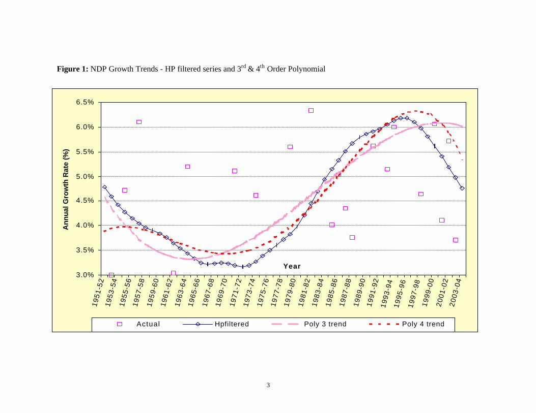
Figure 1 shows the annual growth rate of Net Domestic Product at factor cost
(NDPfc), the growth rate of the Hodrick-Prescott filtered NDPfc series (NDPhp) and the
3rd & 4th order polynomials fitted to the annual growth rate series.3 The NDP growth rate
trend (as measured by the HP-filtered series) started at 4.8% per annum in 1951-2 and
decelerated during the fifties and sixties to reach a low of less than 3.2% per annum
during 1971–72 to 1972–73. The trend growth rate accelerated from the mid-seventies to
reach a peak of almost 6.2% per annum during 1994–95 and 1995–96. Thereafter, the
trend growth rate has decelerated to 4.8% in 2003-4, a rate that is still higher than in
1982-3. The 3rd order polynomial starts in a similar way as the HP filtered series, makes
an earlier trough and then keeps rising even after the HP series has peaked. In contrast
the 4th order polynomial starts much lower and remains flat for some time. Its trough in
the seventies and peak in the nineties is closer to that of the HP filtered series. Because
of these variations with order of the polynomial we prefer to use the HP filtered series for
analysis of growth trends.
3 The NDP series is derived from the published GDP series using the fixed capital series derived by ususing a 5% depreciation rate for capital.
3
Figure 1: NDP Growth Trends - HP filtered series and 3rd & 4th Order Polynomial
3.0%
3.5%
4.0%
4.5%
5.0%
5.5%
6.0%
6.5%1
95
1-5
21
95
3-5
41
95
5-5
61
95
7-5
81
95
9-6
01
96
1-6
21
96
3-6
41
96
5-6
61
96
7-6
81
96
9-7
01
97
1-7
21
97
3-7
41
97
5-7
61
97
7-7
81
97
9-8
01
98
1-8
21
98
3-8
41
98
5-8
61
98
7-8
81
98
9-9
01
99
1-9
2 1
99
3-9
4 1
99
5-9
6 1
99
7-9
81
99
9-0
02
00
1-0
22
00
3-0
4
Year
An
nu
al G
row
th R
ate
(%)
Actual Hpfiltered Poly 3 trend Poly 4 trend
4
Figure 2: Trends in Hodrick-Prescott Filtered Series- NDP, NDPpc & NDPpwrk
0.5%
1.5%
2.5%
3.5%
4.5%
5.5%
6.5%1
95
1-5
21
95
3-5
41
95
5-5
61
95
7-5
81
95
9-6
01
96
1-6
21
96
3-6
41
96
5-6
61
96
7-6
81
96
9-7
01
97
1-7
21
97
3-7
41
97
5-7
61
97
7-7
81
97
9-8
01
98
1-8
21
98
3-8
41
98
5-8
61
98
7-8
81
98
9-9
01
99
1-9
2 1
99
3-9
4 1
99
5-9
6 1
99
7-9
81
99
9-0
02
00
1-0
22
00
3-0
4
Year
An
nu
al G
row
th R
ate
(%)
NDP Per capita Per worker
5
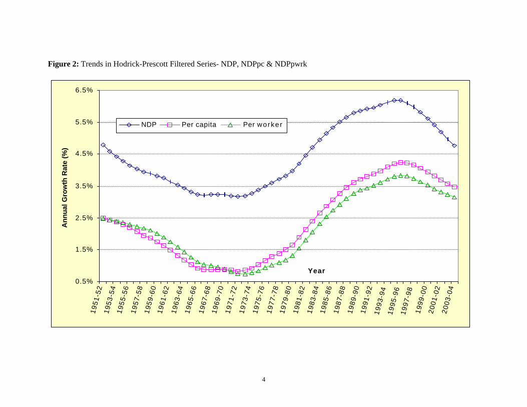
Figure 2 shows the growth trends in Per capita NDPfc (PCndp) and Per worker
NDP (PWndp) along with that in NDPfc.4 Both the per capita and per worker series start
at a trend growth of 2.5% per annum in 1951-2. They reach a trough of 0.7% per annum
in 1971-2 and 0.8% in 1972-3 respectively. Thereafter they rise to a peak of 4.25% and
3.84% respectively in 1995-96. Currently (2003-4) the trend rate is 3.5% per annum in
per capita NDP and 3.1% per annum in per worker NDP.
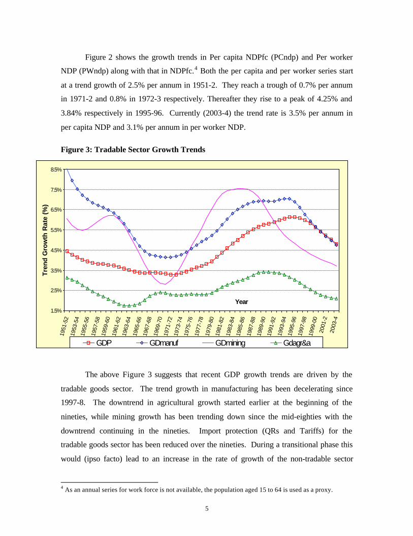
Figure 3: Tradable Sector Growth Trends
The above Figure 3 suggests that recent GDP growth trends are driven by the
tradable goods sector. The trend growth in manufacturing has been decelerating since
1997-8. The downtrend in agricultural growth started earlier at the beginning of the
nineties, while mining growth has been trending down since the mid-eighties with the
downtrend continuing in the nineties. Import protection (QRs and Tariffs) for the
tradable goods sector has been reduced over the nineties. During a transitional phase this
would (ipso facto) lead to an increase in the rate of growth of the non-tradable sector
4 As an annual series for work force is not available, the population aged 15 to 64 is used as a proxy.
1.5%
2.5%
3.5%
4.5%
5.5%
6.5%
7.5%
8.5%
1951
-52
1953
-54
1955
-56
1957
-58
1959
-60
1961
-62
1963
-64
1965
-66
1967
-68
1969
-70
1971
-72
1973
-74
1975
-76
1977
-78
1979
-80
1981
-82
1983
-84
1985
-86
1987
-88
1989
-90
1991
-92
199
3-94
199
5-96
199
7-98
1999
-00
2001
-220
03-4
Year
Tre
nd
Gro
wth
Rat
e (%
)
GDP GDmanuf GDmining Gdagr&a
6
relative to that of the tradable sector. This has indeed happened. The apparent decline in
the trend rate of growth of the tradable goods sectors (manufacturing, mining and
agriculture) over the last 5-7 years is however disturbing and points to the need for
domestic reforms related to these sectors (Virmani (2004b) and references therein).
3 METHODOLOGY
3.1 Sources of Growth
We can use the standard growth accounting framework to apportion growth
between capital accumulation, labour supply and total factor productivity growth. For
this purpose we make the conventional assumption of a constant returns to scale
production function F. Because of the importance of rainfall to the Indian economy we
include rainfall in the production function, assuming that its effect is multiplicative and
factor neutral:
Equation 1: Yt = At G(rainfall) F (Kt, Lt) and yt = At G(rainfall) f(kt)
where, Yt = NDPfc(t), At is neutral technical change, Kt = Capital stock, Lt = Labour,
yt = Yt/Lt (NDPfc per unit of labour), kt = Kt/Lt (Fixed capital per unit of labour).
Rainfall is an area-weighted index of monsoon rainfall all over India. If we assume the
fulfilment of the competitive marginal product conditions we would need the share of
wages and returns to capital. Because of the large size of the unorganised/self-employed
sector as much as 45% of total income is classified as mixed income (labour and capital)
in the National accounts statistics. A time series for labour/capital income shares is
consequently not available. We therefore assume a Cobb-Douglas production function
and on differentiation of Equation 1, obtain the estimating equation,
Equation 2: Gry = C + αα *Grk + E*Drainm + e* Drainm(-1) +Ut
Where Gry is the rate of growth of y, Grk is the rate of growth of k, Drainm is the percent
variation of rainfall from mean with Drainm(-1) representing the lagged value of the
same and Ut is the error term. At is commonly set at C when estimating the coefficients of
Equation 2. The most direct and immediate effect of rainfall is on crop output and
agricultural GDP. The change in the amount of water available in hydel reservoirs also
7
affects electricity generation. The change in availability of surface water also affects the
demand for electricity for drawing sub-surface water. The change of income of farmers
would, also affect the aggregate pattern of demand and consequently the sectoral pattern
of supply. Earlier studies ignore rainfall and therefore include only the first two terms of
Equation 2. This could give biased estimates of elasticity and consequently an under
estimate of TFPG.
Once we have obtained the coefficients of this equation, we can calculate the
Total factor productivity growth (TFPG) as,
Equation 3: TFPG = Gry –αα *Grk –E*Drainm – e*Drainm(-1)
The analysis of the previous section suggests that Growth rate of At could also
equal C0 + C1*Dummy.
If we have constant returns to scale production function without rainfall,
competitive factor markets and a capital share of α, then TFPG would be as follows:
Equation 4: tfpg = Gry – αα *Grk
Thus we can obtain an alternative estimate of tfpg using any value of α. The
estimate obtained by inserting the coefficients estimated in Equation 2 into Equation 3
(TFPG0), however, has one weakness. The entire error term in the GDP growth equation
is attributed to/contained within this estimate. We therefore need to use some smoothing
operation such as the Hodrick-Prescott filter to purge the series of the error term and
derive the underlying trend (TFPG0hp). If TFPG does not have the form C0 +
C1*Dummy and has varied over time because of changes in the policy environment, the
estimate in equation could also be biased. We therefore follow a two-stage procedure.
The filtered series (TFPG0hp) is inserted back into Equation 2 to obtain the following
equation:
Equation 5: Gry = TFPG0hp + αα ’*Grk + E’*Drainm + e’* Drainm(-1) +ut
This equation is estimated to obtain revised values for the co-efficient which are then
used in equation Equation 3 to derive another value for TFPG (TFPG1). The HP filtered
8
version of this (TFPG1hp) then shows the time trend in TFPG. Period averages are,
however, obtained by averaging the unfiltered series (TFPG0 or TFPG1).
3.2 Determinants of TFPG
The link between investment, capital and growth is the foundation of the standard
sources of growth methodology. If technology is capital augmenting, Equation 1 is
modified as follows:
yt = At G(rainfall) f(bt kt) = (At bt)α ktα G(rainfall)
assuming a Cobb-Douglas form. In this case the estimating equations for TFPG remain
unchanged. If technology is embodied in capital stock each vintage of capital has
different productivity and the measurement of aggregate capital stock requires either the
relative price of each vintage or the relative quality. 5 Such information is not available in
India.
De Long and Summers (1991, 1992) have emphasised the link between equipment
investment and growth. They also showed that equipment prices and equipment
investment are inversely related. If technology is embodied in equipment (and not in
structures Kst), augmentation would occur primarily in the machinery & equipment part
of the capital stock (Kmt). It would therefore be necessary to separate out the two forms
of capital in the production function:
yt = At G(rainfall) f(btkmt, kst) = (At btα1) kmt
α1 kstα2 G(rainfall)
De Long and Summers also found that equipment imports are the best predictor of
equipment investment. In a 1993 paper they showed that the effect of equipment
investment is primarily through TFPG. Hulten (1993) showed that for capital goods with
embodied technology, improvements in quality could explain 20% of the residual
(TFPG). Lee (1995) modelled the effect of capital imports and showed that if trade
reduces the price of investment and increases real investment there will faster investment
and technological progress. Thus TFPG may be a function of total or imported
equipment investment or their ratio to total capital stock in Equation 1.
yt = A(Iimpt/I, Imet/I, t)G(rainfall) f(kt)
yt = At (Kmet/Kt )α1 ktα G(rainfall) or yt = At (Kimpt/Kt )α1 kt
α G(rainfall)
5 Hulten (1992), Good, Nadiri, Sickles(1996), Greenwood, Hercowitz & Krusell(1997), Lutz (2000).
9
In the developing country context where technical change is largely a consequence of
diffusion of technology from the developed countries, most embodied technology would
enter through imported capital goods. Technological change could also be affected by the
variety of manufactured intermediates available to the producers. Restrictions on the
import of capital good and intermediate inputs and the tariffs imposed on them would
therefore influence import of these goods and the rate of technological change.6 Such
import policy restrictions would also lead to an appreciation of the real exchange rate
(XRreal= Pt/Pnt, P=price, t=tradables & nt=non-tradables). Changes in the real exchange
rate would capture both the price wedges introduced by QRs & tariffs and the quality
differential between domestic and imported capital goods & intermediates. Thus
technical change could be inversely related to the real exchange rate (i.e. an appreciation
of the exchange rate is correlated with lower TFPG).
Because of the difficulty of estimating augmented capital stock we assume for our
estimation that technological change is either neutral or labour augmenting. TFPG (At in
Equation 1) is a function H of investment in machinery & equipment and of changes in
import restrictions captured by the growth of the real exchange rate (GrXRreal), i.e.
Equation 6: TFPG = H(Ime t/I, GrXRreal, t)
3.3 TFPG by Sector
Equation 4 is also the method used for calculating the TFPG for each sector of the
economy based on an estimate of the capital share (α) for that sector. The contribution of
TFPG in each sector to aggregate/overall TFPG is estimated as follows (the time sub-
script t is dropped):
Y = A F (K , L) or A = Y/F(K, L),
n nY = ∑ Yi = ∑Ai Fi(Ki , Li) i=1 i=1
Substituting the second equation in the first we have,
nA = ∑ Si Ai , and Si = Fi(Ki , Li) / F(K,L) = Ki
αi Li1-αi /Kα L1-α
i=1
6 See also Mazumdar (1996), Connaly (2003).
10
is the ration of total factor input in sector i to total factor input (TFI) into aggregate GDP.
Differentiating this equation with respect to time we have,
nEquation 7: dA = ∑∑ ( Si dAi + A i dSi )
i=1
The term on the left represents the change in total factor productivity of aggregate
GDP. The first term on the right represents the contribution of sectors’ TFPG and the
second term the contribution of the change in allocation of total factor input among
different sectors. The TFPG of sector i contributes a proportion Si dAi /dA to total TFPG
while the factor shift to sector i contributes Ai dSi /dA. If dA is close to zero or negative
this fraction can be misleading and it is better to use the absolute numbers Si dAi and A i
dSi to compare the relative contribution of different sectors.7
4 Empirical Estimation
4.1 Data
The capital stock series is constructed using fixed investment at constant 1993-4
prices from the National Account Statistics (NAS), using the perpetual inventory method.
The depreciation rate is assumed to be 5%. Starting stock (end 1950-1) is also obtained
from the National Account Statistics. The same depreciation values are also used to
construct Net Domestic Product from Gross Domestic Product at factor cost. As an
annual labour or worker series is unavailable we use the population aged 15 to 64 to
measure potential workers for L. This data is obtained from the World development
indicators (from 1960 onwards) and from the UN for 1950. The data for the rest of the
fifties is constructed by interpolation of the ratio of population 15 to 64 over the total
population.
The data problems are more severe when we move from the aggregate to the
sector level. Time series on number of workers or worker hour are not available even at
the aggregate level. We however, have data from national census and National sample
surveys on the number of workers for about nine distinct years for most sectors. The
important exception is Insurance, Banking, Housing Real estate and Business services,
11
which is put in the residual category along with Government and Social & personal
services. Approximately consistent series can be constructed for eight of these years
based on the work of earlier authors.8 Capital share values (α) for all sectors can be
derived from Brhamananda (1982). Based on GDP data and the fixed capital series
constructed by us, we can calculate total factor productivity growth rates by sector for
these seven periods using Equation 4 (These are given in the Appendix table A2).9
These years do not however coincide with the turning points identified in the
aggregate data. Nor do they coincide with the phases and sub-phases of growth identified
in Virmani (2004a). To get an idea of the cyclical trends (peaks, troughs and periods of
rising or declining productivity) we interpolate the share of workers by sector for the
missing years and use the population of 15 to 64 year olds to interpolate the total workers
for the missing years. This is then used along with the GDP data and the capital series to
derive annual TFPG estimates for each sector (from 1952-53 to 2000-01) using capital
share values (α) in Equation 4.10 This allows us to estimate the average productivity
growth during the phases and sub-phases of growth identified earlier.11 We then filter the
TFPG series using an HP filter to find the trend in TFPG and then compare these trends
as represented by the fitted line.
4.2 Production Function and TFPG
OLS estimates of Equation 2 yields the following result:12
Equation 8 : Gry = 0.0148+ 0.430*Grk + 0.202*Drainm – 0.118 * Drainm(-1)
(2.35)** (1.6)* (5.7)*** (-3.4)***
R2 = 0.51, R2 (adj) = 0.48, DW = 2.29. When the Equation 8 is re-estimated with AR(1),
the coefficient on the AR term is not significant. The negative parameter on previous
7 This is what happens in sub-phase IB.8 We use Krishnamurthy (1970) for 1951 & 1961, Sundaram (2001) for 1993-4 & 1999-2000 and Sharma (1997) for the rest.9 The same depreciation rate of 5% is used for all sectors. The cobb-douglas capital co-efficient on totalgdp is taken as estimated earlier (0.42). Sector estimates are derived from simple regression on nine valuesand cross-checked against Brahmananda (1982).10 The income share for the residual sector is derived by subtracting the sum of wages/NDP from sectorsfrom total wages/NDP.11 We then average these over the 7 original periods and compare as a cross-check (appendix A2).12 The numbers in bracket are t-statistics. The level of significance is represented by * (10%), ** (5%) and*** (1%).
12
years’ (lagged) rainfall deviation indicates that the short run (one year) effect of rainfall
deviation on growth (2/10th of rainfall deviation) is higher than the long-term (two-year)
effect (less than 1/10th of rainfall deviation). This is probably due to substitution on both
supply side (e.g. agricultural imports, thermal electricity generation) and demand side
(e.g. income transfers from government or food for work programs) that take time to
adopt.
These parameters are substituted into Equation 3 and TFPG0hp estimated.
TFPG0hp is then used to estimate Equation 5. The results are as follows;
Equation 9:
Gry = 1.11 TFPG0hp + 0.34*Grk + 0.22*Drainm – 0.12 * Drainm(-1) - 0.35*AR(1)
(4.6)*** (1.9)* (6.9)*** (-4.0)*** (-2.5)***
R2 = 0.62, R2 (adj) = 0.59, DW = 2.1.
The most important change is the reduction in the capital coefficient (implicit
profit/capital share). This estimate is almost identical to the capital share (0.35) used by
Collins and Bosworth (1996) and by Guha-Khasnobis and Bari (2003).13 It however
differs from that of Brahmananda (1982), who estimated the share of wages in total
income for the economy as 75% from 1950 to 1970 and 71% for 1980. This suggests a
capital share of 25% in the fifties and sixties, rising to 29% between 1970 and 1980 and
perhaps even higher in the nineties. Our estimate of 0.34 therefore appears quite
reasonable. These new coefficients are reinserted into Equation 3 to get a second
estimate of total factor productivity (TFPG1). This is again smoothed using the Hodrick-
Prescott filter to obtain the trend value (TFPG1hp).14
If we estimate the same regressions using GDP growth as the dependent variable
instead of NDP growth the estimated total factor productivity and its trend (as per the HP
13 The latter was based on Nehru and Dhareshwar (1993)14 If a third stage estimate is done using tfpg1hp the co-efficient on capital per worker falls to 0.239 andbecomes insignificant i.e. there is no convergence.
13
filtered series is virtually the same.15 However the filtered total factor productivity series
using GDP is everywhere below the filtered TFPG series derived using NDP.16
If Equation 4 is used (instead of Equation 3) to estimate TFPG (tfpg0a) and the HP
filtered series (tfpg0ahp) used in the estimation of Equation 5, we obtain
Equation 10:
Gry = 1.04 TFPG0ahp + 0.41*Grk + 0.21*Drainm – 0.13 * Drainm(-1) - 0.32*AR(1)
(4.3)*** (2.4)** (6.4)*** (-4.2)*** (-2.3)***
R2 = 0.61, R2 (adj) = 0.58, DW = 2.1.
There are two noticeable differences from the estimates obtained using tfpg0hp. One, the
co-efficient on the capital per worker appears to be different from that obtained in
Equation 9 (0.411 instead of 0.337) and is significant at a higher level of confidence (2%
instead of 6%). Two, there is virtually no difference in the co-efficient on the capital per
worker from that obtained in Equation 8 (0.43).17 The estimates that use the tfpg
calculated without subtracting the effect of rain fall on ndp growth (0.41) are close to that
of Senhadji (1999) who obtains an estimate of 0.42 for the capital share in case of South
Asia (when estimated in difference form). These estimates contrast both with our
previous estimate of 0.33 and with the non-labour share (0.25 to 0.29) estimated by
Brahmananda (1982).
5 ANALYSIS & IMPLICATIONS
5.1 Productivity Trends
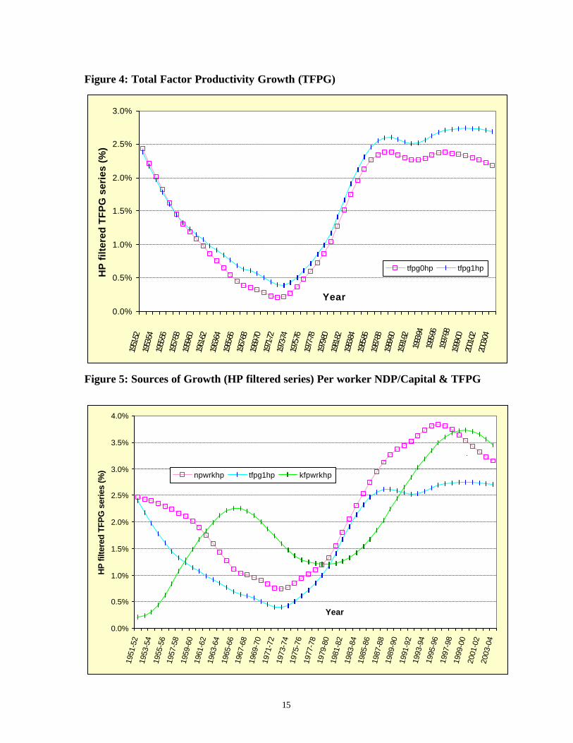
The values of total factor productivity obtained above (TFPG0, TFPG1) are
plotted in Figure 4 in filtered form (TFPG0hp, TFPG1hp). The two HP filtered series for
TFPG follow a broadly similar pattern, though TFPG1hp is found to be higher than
TFPG0hp for all years except the first half of the fifties. Total factor productivity growth
started at 2.4% after independence, but was on a declining trend thereafter. TFPG fell
below single digit at the beginning of the sixties and bottomed out at 0.39% per annum in
15 Significance tend to be somewhat higher however. Thus in borderline cases the regressions using GDPgrowth may be significant at the 10% confidence level but not those using NDP growth.16 By about 1/8th .17 In other words there is greater convergence.
14
1972-73 (TFPG1hp). TFPG has accelerated steadily during the seventies and the eighties
and peaked at 2.62% in 1988-89. This was followed by a temporary setback due to the
BOP crises after which TFPG has essentially plateaued out at around 2.7% per annum
since 1996-97(Figure 4).18
The significant decline in TFPG during mid-sixties to the end-seventies can also
be confirmed directly by the introduction of a dummy variable for the period 1965-66 to
1980-81 (D6580) into Equation 8:
Equation 11:Gry=0.021-0.020*D6580+0.41*Grk+0.21*Drainm–0.15*Drainm(-1)-0.3 AR(1)
(3.9)*** (3.5)*** (2.0)* (6.0)*** (-4.4)*** (2.2)**
R2 = 0.61, R2 (adj) = 0.57, DW = 2.1 .
Equation 11 suggests that TFP growth which averaged about 2.1 per cent per
annum during the over fifty year period, fell by 2.0 per cent points to almost zero during
1965-66 to 1980-81. Virmani (2004a) showed that other exogenous factors such as oil
prices do not have a significant effect on GDP growth and therefore the effect of the
dummy variables could be interpreted as the effect of the set of policies undertaken
during the sub-period. These policies included a comprehensive control regime for the
private sector that can be named Legislative-bureaucratic socialism (popularly known as
‘Licence-Permit-Quota Raj’ and ‘Inspector raj’), which affected not just manufacturing
but all areas of business. Even agriculture was not left untouched as the Essential
commodity act and other restrictions on trade, transport, sale and processing affected
agricultural growth. 19 These along with the after effects of the public monopoly created
till the mid-sixties seem to have played a role in the decline in productivity during 1965-6
to 1979-80.
18 The TFPG0hp series in contrast shows a peak of 2.4% per annum in 1996-97 and a decline to 2.2% perannum at the current time.19 See for instance Virmani and Rajeev (2002) or Virmani (2004b).
15
Figure 4: Total Factor Productivity Growth (TFPG)
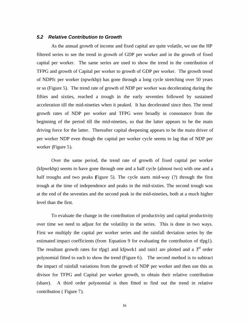
Figure 5: Sources of Growth (HP filtered series) Per worker NDP/Capital & TFPG
0.0%
0.5%
1.0%
1.5%
2.0%
2.5%
3.0%
1951
-5219
53-54
1955
-5619
57-58
1959
-6019
61-62
1963
-6419
65-66
1967
-6819
69-70
1971
-7219
73-74
1975
-7619
77-78
1979
-8019
81-82
1983
-8419
85-86
1987
-8819
89-90
1991
-92
1993
-94
1995
-96
1997
-9819
99-00
2001
-0220
03-04
Year
HP
filt
ered
TF
PG
ser
ies
(%)
tfpg0hp tfpg1hp
0.0%
0.5%
1.0%
1.5%
2.0%
2.5%
3.0%
3.5%
4.0%
1951
-52
1953
-54
1955
-56
1957
-58
1959
-60
1961
-62
1963
-64
1965
-66
1967
-68
1969
-70
1971
-72
1973
-74
1975
-76
1977
-78
1979
-80
1981
-82
1983
-84
1985
-86
1987
-88
1989
-90
1991
-92
199
3-94
199
5-96
199
7-98
1999
-00
2001
-02
2003
-04
Year
HP
filte
red
TFP
G s
erie
s (%
)
npwrkhp tfpg1hp kfpwrkhp
16
5.2 Relative Contribution to Growth
As the annual growth of income and fixed capital are quite volatile, we use the HP
filtered series to see the trend in growth of GDP per worker and in the growth of fixed
capital per worker. The same series are used to show the trend in the contribution of
TFPG and growth of Capital per worker to growth of GDP per worker. The growth trend
of NDPfc per worker (npwrkhp) has gone through a long cycle stretching over 50 years
or so (Figure 5). The trend rate of growth of NDP per worker was decelerating during the
fifties and sixties, reached a trough in the early seventies followed by sustained
acceleration till the mid-nineties when it peaked. It has decelerated since then. The trend
growth rates of NDP per worker and TFPG were broadly in consonance from the
beginning of the period till the mid-nineties, so that the latter appears to be the main
driving force for the latter. Thereafter capital deepening appears to be the main driver of
per worker NDP even though the capital per worker cycle seems to lag that of NDP per
worker (Figure 5).
Over the same period, the trend rate of growth of fixed capital per worker
(kfpwrkhp) seems to have gone through one and a half cycle (almost two) with one and a
half troughs and two peaks (Figure 5). The cycle starts mid-way (?) through the first
trough at the time of independence and peaks in the mid-sixties. The second trough was
at the end of the seventies and the second peak in the mid-nineties, both at a much higher
level than the first.
To evaluate the change in the contribution of productivity and capital productivity
over time we need to adjust for the volatility in the series. This is done in two ways.
First we multiply the capital per worker series and the rainfall deviation series by the
estimated impact coefficients (from Equation 9 for evaluating the contribution of tfpg1).
The resultant growth rates for tfpg1 and kfpwrk1 and rain1 are plotted and a 3rd order
polynomial fitted to each to show the trend (Figure 6). The second method is to subtract
the impact of rainfall variations from the growth of NDP per worker and then use this as
divisor for TFPG and Capital per worker growth, to obtain their relative contribution
(share). A third order polynomial is then fitted to find out the trend in relative
contribution ( Figure 7).

17
Figure 6: Sources of Growth in Per Worker NDP
Figure 7: Contribution to Growth of Per worker NDP (adjstd for rainfall deviation)
-0.5%
0.0%
0.5%
1.0%
1.5%
2.0%
2.5%
3.0%
3.5%
4.0%
4.5%
1951
-52
1953
-54
1955
-56
1957
-58
1959
-60
1961
-62
1963
-64
1965
-66
1967
-68
1969
-70
1971
-72
1973
-74
1975
-76
1977
-78
1979
-80
1981
-82
1983
-84
1985
-86
1987
-88
1989
-90
1991
-92
199
3-94
199
5-96
199
7-98
1999
-00
2001
-02
2003
-04
Year
Ann
ual G
row
th/tr
end
grow
th (%
)
ndppwrk tfpg1 kfpwrk1 rain1
Poly. (ndppwrk) Poly. (tfpg1) Poly. (kfpwrk1) Poly. (rain1)
0.0
0.1
0.2
0.3
0.4
0.5
0.6
0.7
0.8
0.9
1.0
1955
-56
1957
-58
1959
-60
1961
-62
1963
-64
1965
-66
1967
-68
1969
-70
1971
-72
1973
-74
1975
-76
1977
-78
1979
-80
1981
-82
1983
-84
1985
-86
1987
-88
1989
-90
1991
-92
199
3-94
199
5-96
199
7-98
1999
-00
2001
-02
2003
-04
Year
5 ye
ar m
ovin
g av
erag
e (%
)
kfpwrk1 tfpg1 Poly. (kfpwrk1) Poly. (tfpg1)
18
The dotted line at the top of Figure 6 shows the trend in the growth of NDP per
worker, while the dashed line just below it is TFPG. The third dashed line shows the
impact of growth of capital per worker. The contribution of TFPG to growth was initially
high and even offset the negative consequence of capital shallowing. As the contribution
of rainfall to growth was positive (though falling) the growth of NDP per worker
accelerated for about five years till the mid-fifties. The contribution of TFPG declined
over time while that of capital deepening increased. As the deceleration of TFPG was
sharper than the acceleration in capital deepening the growth of NDP per worker
decelerated after the mid-fifties. The acceleration in growth of capital per worker was
driven by a sharp rise in public investment, which more than tripled the public share of
fixed capital from about one tenth (1/10th) in 1950-51 to more than one third (1/3rd) of
total by 1964-65. Public investment was clearly not driven by the profit motive, but the
increase in poverty during this period suggests that the social benefit-cost ratio for this
investment (whether borrowed or raised through distorting taxes) was also low. The low
productivity of this public capital formation appears to have pulled down total factor
productivity growth.
The position was therefore reversed between 1960-1 and 1970-71 when TFPG
was at a trough. During this period capital deepening contributed marginally more than
TFPG to the growth of NDP per worker. The economic situation worsened from the mid-
sixties with the growth of capital stock declining, slowly at first and then in an
accelerating downtrend till the late seventies where it reached a trough. Since 1971-2, the
contribution of TFPG has progressively increased relative to that of capital deepening till
the mid-nineties after which it has declined marginally/stabilised. The contribution of
rain also became negative from 1971-2. Growth of NDP per worker therefore
decelerated till the mid-seventies, picking up only after the decline rate of growth of
capital per worker slowed and the TFPG accelerated.
The relative contribution of TFPG and Capital deepening to the growth of NDP
per worker adjusted for rainfall deviations is depicted in Figure 7. The contribution of
TFPG fell from about 85% at the beginning of the period to 50% in the mid-seventies
while that of capital deepening rose from 15% to 50%. The relative contribution of
19
capital deepening continued to rise till the end of the eighties when it peaked at around
75% and that of TFPG reached a trough of 25%. Since then the contribution of capital
deepening has declined to a little over 52% while that of TFPG has declined to a little
less than 48%. From the trend s it seems likely that the contribution of TFPG will move
above 50% over the next few years, while that of capital deepening will fall.
5.3 TFPG During Growth Phases Virmani (2004a) showed that there were two statistically distinguishable phases
of growth: I) Indian version of socialism (1950-51 to 1979-80) and II) Market Reforms
(1980-1 to present). It also highlighted four sub-phases: IA Quest for commanding
heights, IB Legislative –Bureaucratic Socialism, 20 or socialist rate of growth, IIA modest
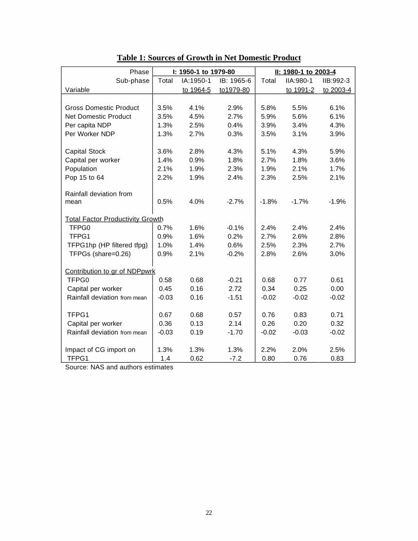
reforms and IIB broader reforms. Table 1 shows the average growth rates and TFPG
estimates in terms of these phases and sub-phases. The average rates of growth of GDP
and NDP were quite similar over the periods and sub periods, so that the conclusions
regarding the sources of growth of NDP per worker and NDP per capita would also apply
to GDP per worker.
One striking contrast that emerges is as follows. While the rate of growth of NDP
per capita and per worker tripled between the socialist and market phases (from 1.3% to
3.9% and 1.3% to 3.5% respectively), the average rate of growth of capital stock per
worker only doubled (from 1.4% to 2.7%). The growth of NDP per worker accelerated
despite a fall in the average deviation of rainfall from a positive 0.5% in phase I to a
negative 1.8% in phase II. Clearly changes in total factor productivity growth are an
important reason for these paradoxes. Equally striking is the fact growth of NDP per
worker fell from 2.7% in sub phase IA to 0.3% in sub phase IB despite a doubling of the
rate of growth of capital per worker from 0.9% per annum to 1.8% annum. Here rainfall
variation provide part of the explanation, with a positive deviations of 4.0% from mean
during sub-phase IA turning into a negative deviation 2.7% during sub-phase IB.
Turning to the estimates of TFPG, we find that the average TFPG over the periods
and sub-periods as estimated in stage one (TFPG0) and stage two (TFPG1) are very
similar. The largest difference of 0.3% between the two measures occurs in sub-phase IB.
The results are also very similar if we ignore the rainfall effects completely and assume
20
that capital share is equal to 0.26 and use this to calculate TFPG using Equation 4 (TFPGs).
The largest difference in this case is 0.5% in sub-phase IA. However, if we take the
averages of the HP filtered series for TFPG1 (TFPG1hp) the result is different for sub-
phase IB (0.5%) and sub-phase IIA (-0.3%). We will therefore use our preferred measure
TFPG1 in the discussion, supplemented by TFPG1hp.
A tripling of the growth of total factor productivity from 0.9% per annum in the
socialist phase I to 2.7% per annum during the market phase II was clearly the driver in
tripling the rate of growth of NDP per capita over these two phases. Of the 2.2% (3.5%-
1.3%) points increase in growth rate of NDP per worker, 1.8% points were due to the
increase in TFPG1 and 0.4% points due to capital deepening. Consequently the
contribution of TFPG to per worker growth increased from 67% during phase I to 76%
during phase II. As the contribution of rainfall remained virtually unchanged, the
contribution of capital deepening correspondingly declined from 36% to 26% (Table 1).
The reason for the sharp decline in the growth of per worker NDP during the
Socialist rate of growth (IB) also becomes clear. More than half the decline of 2.4%
points between sub-phase IA and IB is the result of a 1.4% point per annum decline in
TFPG1. The rest was contributed by the change from above average to below average
rainfall. Thus almost 6/10th (0.57) of the pathetic growth rate of 0.3% during this sub-
phase was due to TFPG1 with the rest coming from capital deepening, which also
compensated for the negative effect of weather (0.44= 2.14 - 1.7).
The rate of growth of per worker NDP has increased from 3.1% per annum during
sub-phase IIA (moderate reforms) to 3.9% per annum in sub-phase IIB (broader reforms).
TFPG has remained almost unchanged over these two sub-phases increasing marginally
from 2.6% per annum to 2.8% per annum (i.e. by 0.2% point). The growth of capital per
worker has however doubled from 1.8% per annum to 3.6% per annum, contributing
0.6% points to the increase in the increase in growth rate of per worker NDP. As a
consequence the contribution of TFPG to the overall growth declined from 83% during
sub-phase IIA to 71% during sub-phase IIB, while that of capital deepening increased
from 20% to 32%. Thus the broadening and deepening of reforms during the latter phase
seem to have lifted ‘animal spirits’ leading to greater investment and growth. The effect
20 Popularly known as the Licence-Permit-Quota Raj
21
on productivity has been modest if we go by TFPG1, but reasonable if we use TFPG1hp.
In the latter case 0.4% of the 0.9% point increase in NDP per worker between sub-phase
IIA and IIB (44%) is accounted for by TFPG.
We can compare our estimates of total TFPG with those given in Guha-Khasnobis
and Bari (2003). For this purpose we have to create decade averages. Our estimates of
TFPG1 are 1.3% per annum during the 1960s, -0.1% per annum during the seventies and
3.0% per annum (appendix table A1). The estimates based on TFPG0 are marginally
lower.21 Our estimates are therefore close to one of their three estimates in which the
growth rates are 1.2%, -0.4% and 2.5% for the same three decades. The estimates of
King and Levine (1993, 1994) are 0.66, -1.77 and 3.0 and differ most sharply for the
seventies. Our analysis suggests that the TFPG for the seventies is underestimated
because of the missing variable rainfall (which was unfavourable). To some extent the
same caveat applies to the under estimation of TFPG in the sixties, where the other two
estimates of Guha-Khasnobis and Bari (2003) are even lower (0.72 and 0.15).
21 The corresponding estimated based on TFPG0 are 1.1% (1960s), -0.2% (1970s) and 2.8% (1980s)
22
Table 1: Sources of Growth in Net Domestic Product
Phase I: 1950-1 to 1979-80 II: 1980-1 to 2003-4Sub-phase Total IA:1950-1 IB: 1965-6 Total IIA:980-1 IIB:992-3
Variable to 1964-5 to1979-80 to 1991-2 to 2003-4
Gross Domestic Product 3.5% 4.1% 2.9% 5.8% 5.5% 6.1%Net Domestic Product 3.5% 4.5% 2.7% 5.9% 5.6% 6.1%Per capita NDP 1.3% 2.5% 0.4% 3.9% 3.4% 4.3%Per Worker NDP 1.3% 2.7% 0.3% 3.5% 3.1% 3.9%
Capital Stock 3.6% 2.8% 4.3% 5.1% 4.3% 5.9%Capital per worker 1.4% 0.9% 1.8% 2.7% 1.8% 3.6%Population 2.1% 1.9% 2.3% 1.9% 2.1% 1.7%Pop 15 to 64 2.2% 1.9% 2.4% 2.3% 2.5% 2.1%
Rainfall deviation frommean 0.5% 4.0% -2.7% -1.8% -1.7% -1.9%
Total Factor Productivity Growth TFPG0 0.7% 1.6% -0.1% 2.4% 2.4% 2.4% TFPG1 0.9% 1.6% 0.2% 2.7% 2.6% 2.8% TFPG1hp (HP filtered tfpg) 1.0% 1.4% 0.6% 2.5% 2.3% 2.7% TFPGs (share=0.26) 0.9% 2.1% -0.2% 2.8% 2.6% 3.0%
Contribution to gr of NDPpwrk TFPG0 0.58 0.68 -0.21 0.68 0.77 0.61 Capital per worker 0.45 0.16 2.72 0.34 0.25 0.00 Rainfall deviation from mean -0.03 0.16 -1.51 -0.02 -0.02 -0.02
TFPG1 0.67 0.68 0.57 0.76 0.83 0.71 Capital per worker 0.36 0.13 2.14 0.26 0.20 0.32 Rainfall deviation from mean -0.03 0.19 -1.70 -0.02 -0.03 -0.02
Impact of CG import on 1.3% 1.3% 1.3% 2.2% 2.0% 2.5% TFPG1 1.4 0.62 -7.2 0.80 0.76 0.83Source: NAS and authors estimates
23
6 DETERMINANTS OF TFPGA simple regression of the ratio of fixed investment in machinery & equipment to
total fixed investment (Ifme/IF) on TFPG yields a highly significant co-efficient:
Equation 12: TFPG1 = 0.044 Ifme/IF –0.17*GrXRreal–0.271 AR(1) (7.8)*** (-2.77)*** (-2.3)**
R2 = 0.27, R2 (adj) = 0.24, DW = 2.1
GrXRreal is the rate of change of the real exchange rate (measured by ratio of
Implicit GDP deflator for tradable goods/non-tradable services). Thus investment in
machinery & equipment seems to have a productivity enhancing effect in India.22 Drainm
and drainm(-1) are not significant when introduced into this equation for TFPG as
expected, as we have taken account of these in calculating TFPG1 (& tfpg0).23 Similar
results are obtained if the dependent variable is Kfme/kf or if the independent variable is
TFPG0.
Using the co-efficient of 0.044 we can estimate the impact of machinery and
equipment investment on TFPG1. Thus machinery and investment was responsible for an
average 0.18% point, 0.15% point 0.32% point and 0.35% point of TFPG in the sub-
phases IA, IIA and IIB respectively. 24 Thus the contribution of machinery and equipment
investment to TFPG growth increased from phase I to phase II. The contribution of the
real exchange rate was a fraction of this except in sub-phase IB when an appreciation
reduced TFPG by 0.13% point thus nullifying the contribution of machinery investment.
Appreciation reduced the TFPG by 0.05% point and 0.06% point in IIA & IIB
respectively.
From Equation 11 we know that the dummy for 1965-6 to 1980-1 has a significant
effect on TFPG. 25 Introducing this into the above equation we have,
22 The inverse equation shows that tfpg1 has an insignificant effect on the ratio of equipment to investment.23 Though Ifme_if and Kfme_kf are also significant when introduced into the production equation Equation 8 the co-efficient ofcapital stock becomes insignificant.24 As capacity utilisation data is unavailable, the capital series represents installed (and not utilised)capacity.25 When crude oil price growth is introduced into this equation its co-efficient of –0.0147 is significant atthe 5% level (R2(adj)=0.29). However it becomes non-significant when D6580 is added. Further the samevariable is not significant in the production function. This suggests that the oil price increases of 1971 &1979 interacted with other policies to produce the negative effect of oil price increase on TFPG.
24
Equation 13: TFPG1 = -0.01 D6580+ 0.05 Ifme/IF –0.17*GrXRreal – 0.35 AR(1) (-2.5)** (8.9)*** (-2.7)*** (-2.8)***
R2 = 0.35, R2 (adj) = 0.31, DW = 2.1 .
The co-efficient on Ifme/Ifixed is marginally higher than in Equation 12 but
similar.26 Thus in addition to import controls and import substitution policies that
affected machinery investment and the real exchange rate, TFPG was reduced by 1%
point during 1965-6 to 1980-81 due to other polices. In other words approximately 1.1%
point of the 1.45% (0.77%) point decline in TFPG1 (TFPG1hp) during sub-phase IB is
explained by Equation 13 (last 2 lines of Table 1).
One possibility is that the other policies captured by the dummy worked to reduce
capacity utilisation. This is suggested by the rise in the co-efficient on machinery
investment on introduction of the dummy and the doubling of the rate of growth of
capital per worker during sub-phase IB. The policies introduced during this phase could
for instance have reduced the rate of capacity utilisation through the following channels:
(a) Rise in import duties leading to higher prices paid by consumers for domestic
consumer goods and consequent reduction in consumer demand. (b) Higher
(income/excise) taxation and consequent reduction in personal disposable income. (c)
Over-investment by government in the production of goods and services for which there
was no demand from the private sector.27 This is the sub-period of “Legislative-
Bureaucratic socialism” that Virmani (2004a) called the “Socialist Rate of Growth (SRG)
period in which GDP growth plummeted.
26 If Ifme_if is replaced by kfme_kf , R2 and R2 (adj) are marginally greater. Similar results are obtained ifTFPG0 is used instead of TFPG1.27 Purchase and price preference tried to generate demand for such goods and services from other publicsector units, but this was perhaps not sufficient
25
7 SECTOR PRODUCTIVITY TRENDS
7.1 Phase I
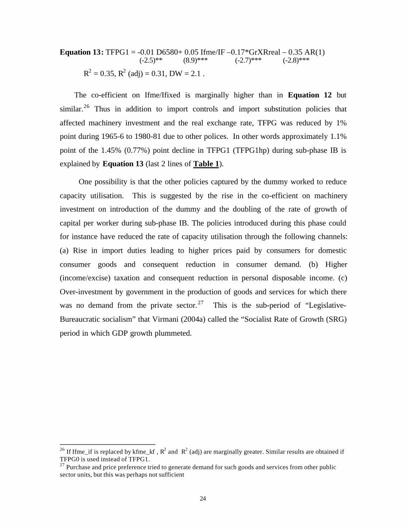
The TFPG estimates for the sectors are summarised in period averages (shown in
tables below) and also presented in the figures below in the form of filtered (using
Hodrick-Prescott filter) series.28 The pattern of TFPG decline in the aggregate series is
most clearly mirrored in the TFPG for Other services (‘Finance, Real estate, housing &
business services’ and ‘Community services & Government administration’) sector and
Trade & Hotels (Figure 8). Except for an initial rise and peak in the TFPG in Trade et al,
the three series decline till the early seventies, with Trade reaching a trough in 1971-72,
aggregate in 1972-3 and Other-services in 1975-76. The TFPG for trade & hotels
however falls much more sharply and becomes negative and then recovers equally
sharply. This suggests problems relating to capacity utilisation perhaps arising from the
negative effect of government appropriating resources from the private individuals and
thus having a negative effect on demand for services. The pattern of growth in private
consumption is found to mirror that in the aggregate TFPG series with the former reaches
a trough in 1970-71(Figure 8), providing support to this hypothesis.
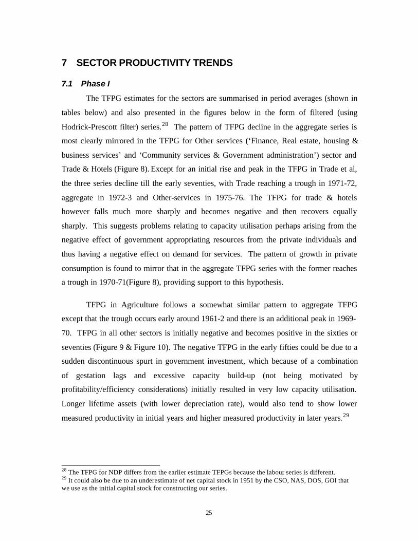
TFPG in Agriculture follows a somewhat similar pattern to aggregate TFPG
except that the trough occurs early around 1961-2 and there is an additional peak in 1969-
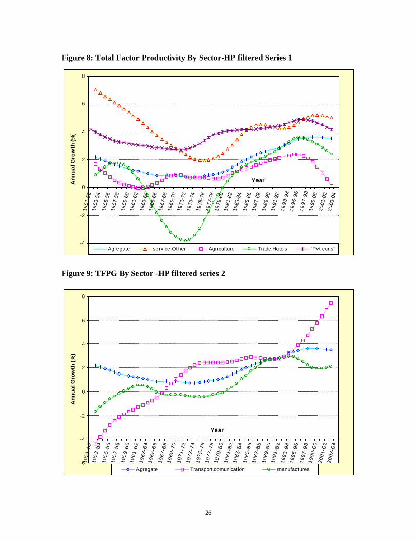
70. TFPG in all other sectors is initially negative and becomes positive in the sixties or
seventies (Figure 9 & Figure 10). The negative TFPG in the early fifties could be due to a
sudden discontinuous spurt in government investment, which because of a combination
of gestation lags and excessive capacity build-up (not being motivated by
profitability/efficiency considerations) initially resulted in very low capacity utilisation.
Longer lifetime assets (with lower depreciation rate), would also tend to show lower
measured productivity in initial years and higher measured productivity in later years.29
28 The TFPG for NDP differs from the earlier estimate TFPGs because the labour series is different.29 It could also be due to an underestimate of net capital stock in 1951 by the CSO, NAS, DOS, GOI thatwe use as the initial capital stock for constructing our series.
26
Figure 8: Total Factor Productivity By Sector-HP filtered Series 1
-4
-2
0
2
4
6
8
1951
-52
1953
-54
1955
-56
1957
-58
1959
-60
1961
-62
1963
-64
1965
-66
1967
-68
1969
-70
1971
-72
1973
-74
1975
-76
1977
-78
1979
-80
1981
-82
1983
-84
1985
-86
1987
-88
1989
-90
1991
-92
19
93
-94
19
95
-96
19
97
-98
1999
-00
2001
-02
2003
-04
YearAn
nu
al G
row
th (%
)
Agregate service-Other Agriculture Trade,Hotels "Pvt cons"
Figure 9: TFPG By Sector -HP filtered series 2
-6
-4
-2
0
2
4
6
8
19
51
-52
19
53
-54
19
55
-56
19
57
-58
19
59
-60
19
61
-62
19
63
-64
19
65
-66
19
67
-68
19
69
-70
19
71
-72
19
73
-74
19
75
-76
19
77
-78
19
79
-80
19
81
-82
19
83
-84
19
85
-86
19
87
-88
19
89
-90
19
91
-92
19
93
-94
19
95
-96
19
97
-98
19
99
-00
20
01
-02
20
03
-04
Year
An
nu
al G
row
th (
%)
Agregate Transport,comunication manufactures
27
Figure 10: Total Factor Productivity By Sector-HP filtered Series 3
-7
-5
-3
-1
1
3
5
7
9
19
51
-52
19
53
-54
19
55
-56
19
57
-58
19
59
-60
19
61
-62
19
63
-64
19
65
-66
19
67
-68
19
69
-70
19
71
-72
19
73
-74
19
75
-76
19
77
-78
19
79
-80
19
81
-82
19
83
-84
19
85
-86
19
87
-88
19
89
-90
19
91
-92
19
93
-94
19
95
-96
19
97
-98
19
99
-00
20
01
-02
20
03
-04
Year
An
nu
al G
row
th (
%)
Agregate Mining construction electricity,gas,water
28
These factors seem to be responsible for the negative TFPG in electricity, mining
and transport (road, rail) & communications and construction during the first decade of
independence as there was a rapid increase in investment during this period. But this also
means that actual TFPG was even lower during sub-phase IB (1965-6 to 1979-80) than
our estimates because of the effect of gestation lags and longer lifetime arising from
investment in sub-phase IA. Put another way, given the sharp slowing of investment in
sub phase IB neglect of these two factors would mean that TFPG is overestimated.
As long as sector TFPG is negative it clearly pulls down aggregate TFPG. TFPG
in Transport-communications and electricity generally follow a rising trend with
intervening plateau. The trend TFPG in Manufacturing, Mining and Construction made a
trough at a negative value in 1974-75, 1979-80s and 1983-84 respectively, after which
TFPG rose. The electricity sector has also been on a rising trend since 1978-79.
The TFPG trend (HP filtered series) for manufacturing was positive for only 8 out
of the 30 years from 1950-1 to 1979-80 (phase I) mostly during sub-phase IA. According
to the unfiltered series TFPG averaged 0.4% in sub-phase IA and –0.3% in phase I as a
whole. It was therefore effectively zero during this period of “Socialism with and Indian
face,” characterised by the Mahalanobis model of state led heavy industry (machines for
making machines) complemented by small-scale industry reservation. 30
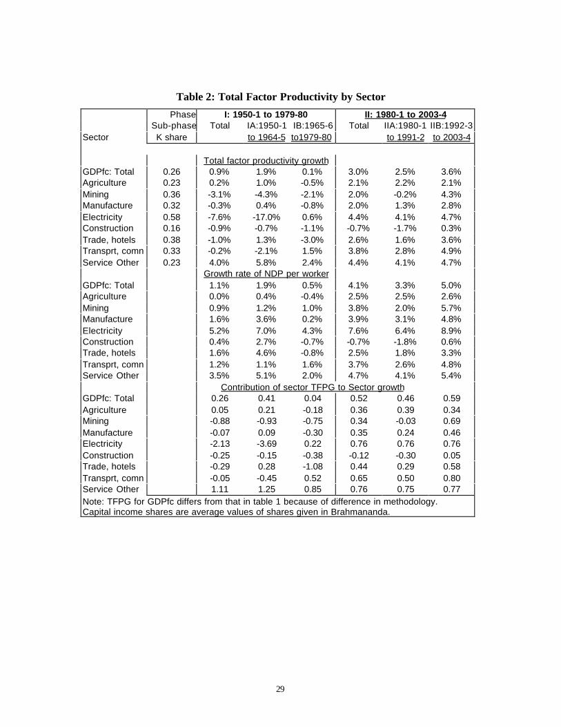
Given this pattern of TFPG trends in Phase I (1950-1 to 1979-80), TFPG was
negative in all sectors except agriculture and the residual sector ‘Other services’ (Table 2).
While agriculture TFPG was positive in sub-phase IA alone, TFPG in ‘Other services’
grew strongly in both phases. As a result TFPG was the sole cause of growth of other-
service during sub-phase IB, overcoming even some capital shallowing. In sub-phase IB
TFPG was responsible for 85% of the growth with the result that during phase I as a
whole TFPG contribution was more than 100%. Given the size of these two sectors, this
was sufficient to ensure that aggregate TFPG was positive, with a little help from a
positive TFPG in ‘Manufacturing’ and ‘Trade, Hotels & Restaurants’ in sub-phase IA
and a positive TFPG in ‘Electricity, Gas & Water’ and ‘Transport and communications’
in sub-phase IB.
30 I.e. data limitations do not allow us to distinguish TFPG from zero..
29
Table 2: Total Factor Productivity by Sector
Phase I: 1950-1 to 1979-80 II: 1980-1 to 2003-4Sub-phase Total IA:1950-1 IB:1965-6 Total IIA:1980-1 IIB:1992-3
Sector K share to 1964-5 to1979-80 to 1991-2 to 2003-4
Total factor productivity growthGDPfc: Total 0.26 0.9% 1.9% 0.1% 3.0% 2.5% 3.6%Agriculture 0.23 0.2% 1.0% -0.5% 2.1% 2.2% 2.1%Mining 0.36 -3.1% -4.3% -2.1% 2.0% -0.2% 4.3%Manufacture 0.32 -0.3% 0.4% -0.8% 2.0% 1.3% 2.8%Electricity 0.58 -7.6% -17.0% 0.6% 4.4% 4.1% 4.7%Construction 0.16 -0.9% -0.7% -1.1% -0.7% -1.7% 0.3%Trade, hotels 0.38 -1.0% 1.3% -3.0% 2.6% 1.6% 3.6%Transprt, comn 0.33 -0.2% -2.1% 1.5% 3.8% 2.8% 4.9%Service Other 0.23 4.0% 5.8% 2.4% 4.4% 4.1% 4.7%
Growth rate of NDP per workerGDPfc: Total 1.1% 1.9% 0.5% 4.1% 3.3% 5.0%Agriculture 0.0% 0.4% -0.4% 2.5% 2.5% 2.6%Mining 0.9% 1.2% 1.0% 3.8% 2.0% 5.7%Manufacture 1.6% 3.6% 0.2% 3.9% 3.1% 4.8%Electricity 5.2% 7.0% 4.3% 7.6% 6.4% 8.9%Construction 0.4% 2.7% -0.7% -0.7% -1.8% 0.6%Trade, hotels 1.6% 4.6% -0.8% 2.5% 1.8% 3.3%Transprt, comn 1.2% 1.1% 1.6% 3.7% 2.6% 4.8%Service Other 3.5% 5.1% 2.0% 4.7% 4.1% 5.4%
Contribution of sector TFPG to Sector growthGDPfc: Total 0.26 0.41 0.04 0.52 0.46 0.59Agriculture 0.05 0.21 -0.18 0.36 0.39 0.34Mining -0.88 -0.93 -0.75 0.34 -0.03 0.69Manufacture -0.07 0.09 -0.30 0.35 0.24 0.46Electricity -2.13 -3.69 0.22 0.76 0.76 0.76Construction -0.25 -0.15 -0.38 -0.12 -0.30 0.05Trade, hotels -0.29 0.28 -1.08 0.44 0.29 0.58Transprt, comn -0.05 -0.45 0.52 0.65 0.50 0.80Service Other 1.11 1.25 0.85 0.76 0.75 0.77Note: TFPG for GDPfc differs from that in table 1 because of difference in methodology.Capital income shares are average values of shares given in Brahmananda.
30
There was massive decline in factor productivity in the electricity sector in sub-
phase IA and a substantial decline in productivity in the mining sector in both sub-phases.
Both these sectors were reserved for the government and the share of public sector in
total GDP from these sectors went up to 100% in electricity and about 97% in mining by
the end of phase I. Gestation lags in investment may have been partly responsible for the
mismatch between investment and output, especially in electricity. The government may
also have built capacity too far ahead of potential demand on the assumption that supply
would create demand through general development (Mahalanobis model!).31 The net
result, as in the former USSR, was that nationalisation of these sectors had a negative
effect on TFPG even though GDP from these sectors continued to grow due to capital
deepening and expansion of manpower.
The negative TFPG growth in Manufacturing and in Trade, Hotels & Restaurants
in sub-phase IB could have been due to the following: (a) Declining capacity utilisation.
(b) Use of inferior domestic (import-substituting) capital goods consequent to imposition
of QRs. (c) Use of inferior imported capital goods from the rupee payment areas (Soviet
Union, E Europe) which were exempt from QRs/bans applicable to import of capital
goods from convertible currency areas. The negative TFPG growth in ‘Transport and
Communications’ in sub-phase IA was due partly to the government monopoly of the
railways and communications and partly to the above reasons.
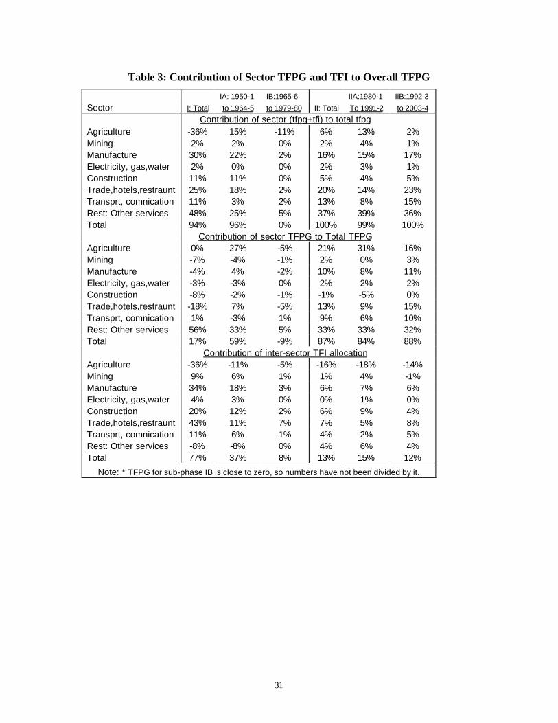
In phase I as a whole TFPG growth in sectors (Table 3 based on Equation 7) was
responsible for about 17% of overall TFPG growth with other services being the main
contributor (56%). The remaining TFPG growth was the result of a shift of factors from
agriculture (33%) and Other-services to all other sectors [Trade & hotels (43%),
Manufactures (34%) and construction (20%)]. In sub-phase IA TFPG growth in sectors
was responsible for almost 60% of total TFPG with agriculture (27%) and other services
contributing almost equally (33%). The remaining contribution came from a shift of
factors out of agriculture and other services to the remaining sectors.
31 A modified/dynamic version of Says law.
31
Table 3: Contribution of Sector TFPG and TFI to Overall TFPG
IA: 1950-1 IB:1965-6 IIA:1980-1 IIB:1992-3
Sector I: Total to 1964-5 to 1979-80 II: Total To 1991-2 to 2003-4
Contribution of sector (tfpg+tfi) to total tfpgAgriculture -36% 15% -11% 6% 13% 2%Mining 2% 2% 0% 2% 4% 1%Manufacture 30% 22% 2% 16% 15% 17%Electricity, gas,water 2% 0% 0% 2% 3% 1%Construction 11% 11% 0% 5% 4% 5%Trade,hotels,restraunt 25% 18% 2% 20% 14% 23%Transprt, comnication 11% 3% 2% 13% 8% 15%Rest: Other services 48% 25% 5% 37% 39% 36%Total 94% 96% 0% 100% 99% 100%
Contribution of sector TFPG to Total TFPGAgriculture 0% 27% -5% 21% 31% 16%Mining -7% -4% -1% 2% 0% 3%Manufacture -4% 4% -2% 10% 8% 11%Electricity, gas,water -3% -3% 0% 2% 2% 2%Construction -8% -2% -1% -1% -5% 0%Trade,hotels,restraunt -18% 7% -5% 13% 9% 15%Transprt, comnication 1% -3% 1% 9% 6% 10%Rest: Other services 56% 33% 5% 33% 33% 32%Total 17% 59% -9% 87% 84% 88%
Contribution of inter-sector TFI allocationAgriculture -36% -11% -5% -16% -18% -14%Mining 9% 6% 1% 1% 4% -1%Manufacture 34% 18% 3% 6% 7% 6%Electricity, gas,water 4% 3% 0% 0% 1% 0%Construction 20% 12% 2% 6% 9% 4%Trade,hotels,restraunt 43% 11% 7% 7% 5% 8%Transprt, comnication 11% 6% 1% 4% 2% 5%Rest: Other services -8% -8% 0% 4% 6% 4%Total 77% 37% 8% 13% 15% 12%
Note: * TFPG for sub-phase IB is close to zero, so numbers have not been divided by it.
32
If we look at the full (TFPG + TFI share) contribution of each sector to total TFPG,
Other service is the largest contributor (I: 48%, IA: 25%) but is followed by
manufacturing (30%, 20%) and Trade, Hotels & Restaurants (25%, 18%). In phase IB the
total TFPG is so small that it is difficult to be sure about the relative contributions (Table
3, column 3).
7.2 Phase II
Since 1980-81 TFPG was negative only in mining and construction till 1987-8
and 1988-89 respectively (Figure 8, Figure 9 & Figure 10). TFPG trend in every sector
except construction (which bottomed out in 1984-5) was rising, with the trend in most
sectors peaking between 1992-3 and 1999-2000. The aggregate TFPG also peaked then.
The first sector TFPG to peak was construction at 1.3% in 1992-3, followed by
manufacturing TFPG at 3% in 1993-4, agriculture TFPG at 2.35% in 1994-5, Trade-
hotels at 3.6% in 1995-6, and electricity (6%) and other-services (5.2%) in 1999-2000.
TFPG in mining (8.2%) and transport-communication (7.5%) is however still on an
accelerating trend as of 2002-3 with the latter driven primarily by the communication
sub-sector. In the case of mining the share of the public sector in GDP and in GCF has
been on a downtrend since the late 1980, so that entry of the private sector could have
contributed to rising TFPG. In the case of the communication sector, policy and
regulatory reform starting with the opening of the sector to private entry and competition
arising from the introduction divisible mobile technologies has clearly fuelled TFPG and
Value added growth. 32
Construction is the only sector in which average TFPG was negative during phase
II (1980-1 to 2002-3). Its performance has been abysmal. Much of construction is either
carried out by government or procured by government. The procurement standards and
procedures adopted by the government therefore play a vital role in the evolution of the
construction industry. These standard and procedures have not been changed since
independence so that the industry has been stuck in a time warp. As noted in Virmani
32 Virmani (2004c) describes Telecom reform as the second most successful reform (after external sectorreform) during the nineties.
33
(2004b), there is an urgent need to modernise procurement and other policies related to
the construction sector.
Between Phase IB (1965-6 to 1979-80) and IIA (1980-1 to 1991-2) TFPG
accelerated most sharply in Trade & hotels and electricity sectors and least in
construction. Transport & communications and Other services, however continued to
have above average growth of TFPG during phase IIA and IIB with the former
accelerating sharply in IIB and the latter also improving from its high levels.
During phase II, the contribution of sector TFPG to the same sector’s GDP per
worker ranged from a low of around 35% in mining, manufacturing and agriculture to
76% in ‘electricity, Gas & water’ and ‘Other services.’ The rest was contributed by
capital deepening. 33 For both electricity and other services the contribution of sector
TFPG to sector’s GDP per worker remained at around 75% in both sub-phases (IIA &
IIB). While in agriculture it varied around 36%, it increased from phase IIA to IIB), in
manufacturing (24%, 46%), Trade, Hotels & Restaurants (29%, 58%) and Transport,
Storage & communications (50%, 80%).
The contribution of sector TFPG to aggregate TFPG increased sharply during phase
II to 87% from the 17% average during phase I and 59% during sub-phase IA. The
greatest increase in contribution was in Trade-hotels, followed by Agriculture and
Manufacturing. The average contribution of TFPG in Other-services declined sharply, but
it remained the largest contributor to aggregate TFPG. The contribution of all other
sectors increased by small amounts. Inter-sectoral shifts in factors contributed only 13%
to aggregate TFPG during phase II (table 3).
The contribution of sector TFPG was marginally lower in sub-phase IIA (84%) and
marginally higher in sub-phase IIB (89%). Compared to Sub-phase IIA, IIB also saw a
smaller contribution from TFPG in agriculture, and a larger contribution from TFPG in
Trade-hotels, construction, transport-communications, manufacturing and mining. In
other words the sector TFPG contributions were more evenly distributed in sub-phase IIB
even though other-services continued to contribute a little less than 33% (Table 3).
33 We are unable to make adjustment for the effect of rainfall on production because of data limitations.

34
TFPG in agriculture has declined sharply during the second half of the nineties
(Figure 8). Among the potential reasons for this sharp decline are: (a) The deterioration in
the fertiliser (NPK) mix because of price distortions arising from subsidies for urea. (b)
Lowering of water table due to inadequate public attention to developing and maintaining
water systems for regenerating underground water and optimal utilisation of surface
water. (c) Over-exploitation of under-ground water because of provision of free
electricity by the State. (d) Deteriorating R&D and extension systems. This highlights
the urgency of reforming policies relating to the entire food chain starting from
production to retailing (Virmani and Rajeev (2002), Virmani (2004b)).
The trend growth of TFPG has, after rising to 2.5% per annum in the mid-nineties,
regressed to 2% per annum. This is less than the aggregate TFPG estimated in the first
part of the paper and is significantly lower than TFPG estimated by applying exogenous
capital shares and ignoring rainfall effects. Thus manufacturing, instead of acting as a
driver of overall TFPG currently appears to be acting as a drag. Economic reforms
related to labour intensive manufacturing should be accelerated to raise TFPG and global
competitiveness of this tradable sector.34
34 See for instance Virmani (1999), Virmani (2000), Virmani (2004b) for a discussion of required reforms.
35
8 CONCLUSION
Since independence trend growth of Gross domestic product (GDP) and Net
domestic product (NDP) has gone through one complete cycle (growth cycle) with a
trough in 1971-72 and a peak in 1994-95. The trend started at around 4.8% per annum in
1951-2 and is currently around the same level. The trends in growth of NDP per capita
and NDP per worker were almost identical. This paper uses the source of growth
methodology to explain this growth cycle. It shows that Total factor productivity growth
followed a V shaped pattern between 1951-2 and 1985-86 with the tip of the V in the
year 1971-2. Since the mid-nineties TFPG has flattened out with a gently rising trend.
Growth of Net domestic product per worker also follows a V shaped pattern but peaks
much later in the mid-nineties and turns down thereafter instead of plateauing out. The
pattern of capital deepening (growth of capital per worker) in contrast is quite different,
with two almost complete cycles. The first peak occurs in 1965-6 and the second one in
1998-9 to 1999-2000, three years after the peak in growth of per worker NDP.
The contribution of total factor productivity growth to growth of Net Domestic
Product per worker (net of effects of variations in rainfall) consequently fell
progressively from 85% in 1951-2 to a little over 25% in 1991-92. The contribution has
risen sharply since then to almost 50% (a level it last had around 1975-6). The
contribution of capital deepening (growth of capital per worker has followed the inverse
pattern. 35
The paper then goes on to link the TFPG estimates to the analysis of growth and
policy structures given in Virmani (2004a). It shows that the collapse of GDP/NDP
growth during the sub-period 1965-6 to 1979-80 (sub-phases IB) was due substantially to
a sharp fall in total factor productivity growth. Half the decline in growth between sub-
phase IA and sub-phase IB was because of the decline in TFPG and the rest because of
poor rainfall. The paper also shows that the recovery of growth during 1980-1 to 1991-2
(sub-phase IIA) was due to an increase in TFPG to 1.6 times the level prevailing in 1951-
35 With the effect of rainfall purged, the two contribution must add up to one even though the smootingprocess may not produce the precise result (i.e. adding up to 100 %)
36
2 to 1964-5 (sub-phase IA) coupled with a doubling of per worker NDP growth relative
to IA. A change of policy direction from an immersion in the Indian version of socialism
towards market economics has been responsible for the acceleration in both these sources
of growth.
Formal econometric analysis shows that investment in machinery (relative to
investment in structures) and changes in protection (through QRs and tariffs) played an
important role in the rate of growth of total factor productivity. It is shown that the ratio
of machinery to total investment and the rate of change in the real exchange rate (ratio of
tradable/goods prices to non-tradable/service prices) have significant effect on TFPG and
explain about 25% of the variation in it. Other policies prevailing during 1965-6 to 1979-
80, captured by a dummy variable, explain another 5-10% of the variation in TFPG
during the entire period from 1951-2 to 2003-4.
The paper goes on to estimate total factor productivity for all major sectors of the
economy for which data on workers is available. This allows us to examine the relative
contribution of TFPG and capital deepening to per worker growth in each sector. The
TFPG estimates are also used to estimate the contribution of each sector’s total factor
productivity growth and capital deepening to growth of aggregate TFPG. It is shown that
the contribution of sector TFPG to aggregate TFPG increased from 17% during 1951-2 to
1979-80 (phase I) to 87% in 1980-1 to 2003-4 (phase II). The greatest increase in
contribution was in ‘Trade, hotels & restaurants’ followed by agriculture and
manufacturing. TFPG in ‘Other services (financial, real estate, housing, business,
personal and govt services) remained the largest contributor to aggregate TFPG (though
the change in it was small). Further, more detailed, work needs to be done to identify the
productivity drivers in the service sectors.
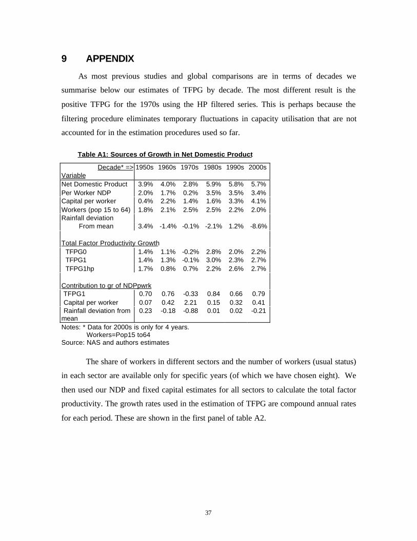
37
9 APPENDIX
As most previous studies and global comparisons are in terms of decades we
summarise below our estimates of TFPG by decade. The most different result is the
positive TFPG for the 1970s using the HP filtered series. This is perhaps because the
filtering procedure eliminates temporary fluctuations in capacity utilisation that are not
accounted for in the estimation procedures used so far.
Table A1: Sources of Growth in Net Domestic Product
Decade* => 1950s 1960s 1970s 1980s 1990s 2000sVariableNet Domestic Product 3.9% 4.0% 2.8% 5.9% 5.8% 5.7%Per Worker NDP 2.0% 1.7% 0.2% 3.5% 3.5% 3.4%Capital per worker 0.4% 2.2% 1.4% 1.6% 3.3% 4.1%Workers (pop 15 to 64) 1.8% 2.1% 2.5% 2.5% 2.2% 2.0%Rainfall deviation From mean 3.4% -1.4% -0.1% -2.1% 1.2% -8.6%
Total Factor Productivity Growth TFPG0 1.4% 1.1% -0.2% 2.8% 2.0% 2.2% TFPG1 1.4% 1.3% -0.1% 3.0% 2.3% 2.7% TFPG1hp 1.7% 0.8% 0.7% 2.2% 2.6% 2.7%
Contribution to gr of NDPpwrk TFPG1 0.70 0.76 -0.33 0.84 0.66 0.79 Capital per worker 0.07 0.42 2.21 0.15 0.32 0.41 Rainfall deviation frommean
0.23 -0.18 -0.88 0.01 0.02 -0.21
Notes: * Data for 2000s is only for 4 years. Workers=Pop15 to64Source: NAS and authors estimates
The share of workers in different sectors and the number of workers (usual status)
in each sector are available only for specific years (of which we have chosen eight). We
then used our NDP and fixed capital estimates for all sectors to calculate the total factor
productivity. The growth rates used in the estimation of TFPG are compound annual rates
for each period. These are shown in the first panel of table A2.
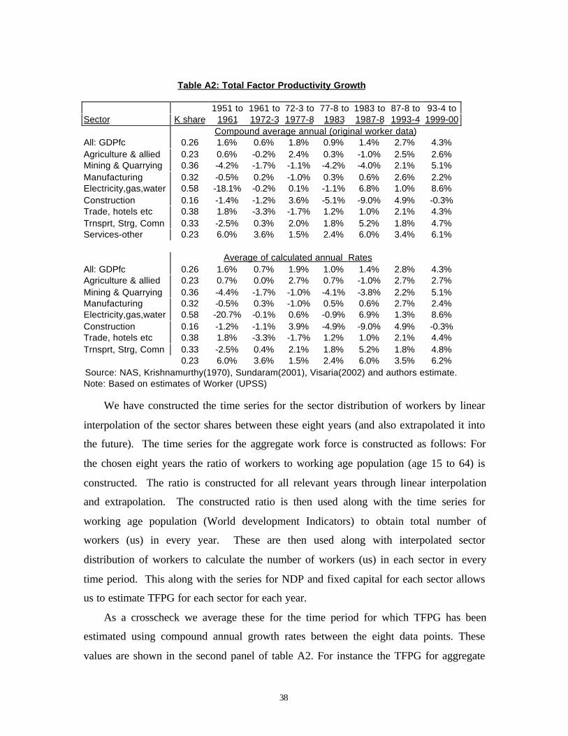
38
Table A2: Total Factor Productivity Growth
1951 to 1961 to 72-3 to 77-8 to 1983 to 87-8 to 93-4 toSector K share 1961 1972-3 1977-8 1983 1987-8 1993-4 1999-00
Compound average annual (original worker data)All: GDPfc 0.26 1.6% 0.6% 1.8% 0.9% 1.4% 2.7% 4.3%Agriculture & allied 0.23 0.6% -0.2% 2.4% 0.3% -1.0% 2.5% 2.6%Mining & Quarrying 0.36 -4.2% -1.7% -1.1% -4.2% -4.0% 2.1% 5.1%Manufacturing 0.32 -0.5% 0.2% -1.0% 0.3% 0.6% 2.6% 2.2%Electricity,gas,water 0.58 -18.1% -0.2% 0.1% -1.1% 6.8% 1.0% 8.6%Construction 0.16 -1.4% -1.2% 3.6% -5.1% -9.0% 4.9% -0.3%Trade, hotels etc 0.38 1.8% -3.3% -1.7% 1.2% 1.0% 2.1% 4.3%Trnsprt, Strg, Comn 0.33 -2.5% 0.3% 2.0% 1.8% 5.2% 1.8% 4.7%Services-other 0.23 6.0% 3.6% 1.5% 2.4% 6.0% 3.4% 6.1%
Average of calculated annual RatesAll: GDPfc 0.26 1.6% 0.7% 1.9% 1.0% 1.4% 2.8% 4.3%Agriculture & allied 0.23 0.7% 0.0% 2.7% 0.7% -1.0% 2.7% 2.7%Mining & Quarrying 0.36 -4.4% -1.7% -1.0% -4.1% -3.8% 2.2% 5.1%Manufacturing 0.32 -0.5% 0.3% -1.0% 0.5% 0.6% 2.7% 2.4%Electricity,gas,water 0.58 -20.7% -0.1% 0.6% -0.9% 6.9% 1.3% 8.6%Construction 0.16 -1.2% -1.1% 3.9% -4.9% -9.0% 4.9% -0.3%Trade, hotels etc 0.38 1.8% -3.3% -1.7% 1.2% 1.0% 2.1% 4.4%Trnsprt, Strg, Comn 0.33 -2.5% 0.4% 2.1% 1.8% 5.2% 1.8% 4.8%
0.23 6.0% 3.6% 1.5% 2.4% 6.0% 3.5% 6.2%Source: NAS, Krishnamurthy(1970), Sundaram(2001), Visaria(2002) and authors estimate.Note: Based on estimates of Worker (UPSS)
We have constructed the time series for the sector distribution of workers by linear
interpolation of the sector shares between these eight years (and also extrapolated it into
the future). The time series for the aggregate work force is constructed as follows: For
the chosen eight years the ratio of workers to working age population (age 15 to 64) is
constructed. The ratio is constructed for all relevant years through linear interpolation
and extrapolation. The constructed ratio is then used along with the time series for
working age population (World development Indicators) to obtain total number of
workers (us) in every year. These are then used along with interpolated sector
distribution of workers to calculate the number of workers (us) in each sector in every
time period. This along with the series for NDP and fixed capital for each sector allows
us to estimate TFPG for each sector for each year.
As a crosscheck we average these for the time period for which TFPG has been
estimated using compound annual growth rates between the eight data points. These
values are shown in the second panel of table A2. For instance the TFPG for aggregate

39
GDP during the period 1951 to 1961 was 1.6% per annum both by the compound annual
average method and by averaging the annual TFPG obtained through interpolation of
worker series. In contrast, the TFPG for the electricity sector between 1972-3 and 1977-
78 is 0.1% per annum by the compound method and 0.6% per annum (or almost six
times) by interpolation method. Overall, except for a few sectors and periods the two sets
of TFPG estimates are quite close.
The decade averages for the annual estimates by sector are summarised in the
appendix table A3.
Table A3: Total Factor Productivity Growth
Period => 1950s 1960s 1970s 1980s 1990s 2000sVariable
All: GDPfc 1.5% 1.4% 0.0% 3.0% 3.1% 3.1%Agriculture & allied 0.6% 0.8% -0.8% 2.8% 2.0% 0.2%Mining & Quarrying -5.7% -0.9% -3.3% -0.6% 3.0% 6.9%Manufacturing -1.1% 0.7% -0.6% 2.2% 1.4% 3.6%Electricity, Gas & Water -27% 0.7% -0.1% 4.1% 4.6% 4.6%Construction -2.0% 0.5% -1.4% -3.2% 1.5% 0.4%Trade, Hotels, etc 1.3% -0.8% -3.1% 2.1% 3.1% 2.1%Transport, Strg, Comn -2.8% -0.4% 2.1% 3.0% 3.5% 7.2%Services-other 6.2% 4.0% 2.1% 4.5% 4.6% 3.3%Note: Based on estimates of Workers (UPSS)
According to this break up, aggregate and sector TFPG growth was the worst
during the seventies, consistent with the available studies. The negative TFPG results for
so many sectors in the 1950s however contradicts the results of Brahmananda. The
results for the 1990s and 2000s are also new, though the latter are very tentative.
40
10 REFERENCES
1. Ahluwalia, Isher Judge, (1985), ‘Industrial Growth in India: Stagnation Since the Mid-Sixties’, OxfordUniversity Press, Delhi.
2. Ahluwalia, Isher Judge, (1991), ‘Productivity and Growth in Indian Manufacturing’, Oxford UniversityPress, Oxford & New York, 1991.
3. Balakrishnan, P., K. Pushpangadan and M. Suresh Babu (2000), “Trade Liberalisation and ProductivityGrowth in Manufacturing: Evidence from Firm Level Panel Data”, Economic and Political Weekly, Oct7, 3679-3682
4. Barik and Pradhan (1999), “Total Factor Productivity Growth in Developing Economies: A Study ofSelected Industries in India”, Economic and Political Weekly, July 31, 1999.
5. Brahmananda, P. R.(1982), Productivity in the Indian Economy: Rising Inputs for Falling Outputs,Himalaya Publishing House, 1982
6. Collins, Susan and Bosworth, Barry (1996), “Economic Growth in East Asia: Accumulation VersusAssimilation”, Brookings Papers on Economic Activity, 2:135-203.
7. Connolly, Michelle (2003), “The Dual Nature of Trade:Measuring its Impact on Imitation andGrowth”, Journal of Development Economics, 72, 31 - 55
8. Das, Deb Kusum (2003), “Manufacturing Productivity under varying trade Regimes: India in the1980s and 1990s.” ICRIER working paper No. 107, August 2003 (www.icrier.org)
9. DeLong, J Bradford and Summers, Lawrence (1991), “Equipment Investment and Economic Growth,”Quarterly Journal of Economics 106 (May 1991), pp 445-502.
10. DeLong, J Bradford and Summers, Lawrence (1992), “Equipment Investment and Economic Growth,How Strong is the Nexus,” Brooking Papeers in Economic Activity, 2, pp 157-99.
11. Edwards, Sebastian (1997) ‘Openness, Productivity And Growth: What Do We Really Know.’ NBER,WP 5978, March 1997.
12. Fagerberg, Jan (1994), “ Technology and International Differences in Growth Rates”, Journal ofEconomic Literature, 32, 1147 – 1175.
13. Goldar, Biswanath (2002), “TFP Growth in Indian Manufacturing in 1980’s” Economic and PoliticalWeekly, Dec 7, 2002, pp 4966 - 4968
14. Goldar, B. and Anita Kumari (2003), “Import Liberalisation and Productivity Growth in IndianManufacturing Industries in the 1990’s”, The Developing Economies, XLI (4), Dec 2003.
15. Goldar, B. and Arup Mitra (2002), “Total Factor Productivity Growth in Indian ManufacturingIndustries in the 1990’s”, in National Accounts and Data Systems, ed. B.S. Minhas, New Delhi:Oxford University Press.
16. Good D.H., M.I. Nadiri and R.C. Sickles (1996), “Index Number and Factor Demand Approaches tothe Estimation of Productivity”, NBER Working Paper No. 5790, Oct 1996
17. Greenwood, J., Zvi Hercowitz and Per Krusell (1997), “Long Run Implications of Investment SpecificTechnological Change”, Americal Economic Review, 87 (3), 342 – 362.
18. Guha-Khasnobis, Basudeb and Bari, Faisal, (2003), ‘Sources of Growth in South Asian Countries’, in‘The South Asian Experience with Growth’, edited by Isher Judge Ahluwalia and John Williamson,Oxford University Press, 2003
19. Hendricks, Lutz (2000), “Equipment Investment and Growth in Developing Countries,” Journal ofDevelopment Economics, 61, (2000), pp335-364.
20. Hulten, Charles R (1992) ‘Growth Accounting When Technical Change is Embodied in Capital,’American Economic Review, 82(4), September 1992, 964-80.
21. International Labour Organization (ILO), (2002), ‘Yearbook of Labour Statistics’, ILO.22. King, R.G and Ross Levine (1993), “Finance, Enterpreneurship and Growth: Theory and Evidence”,
Journal of Monetary Economics, 32, 513-542. Carnegie-Rochester Conference Series on Public Policy.June 1994.
41
23. King, R.G and Ross Levine(1994), “Capital Fundamentalism, Economic Development and EconomicGrowth.”
24. Krishna, P. and D. Mitra (1998), “Trade Liberalization, Market Discipline and Productivity Growth:New Evidence from India"” Journal of Development Economics, 56, 447-62.
25. Krishnamurthy, J. (1970) "Industrial Distribution of the working force in India, 1901-1961: A study ofselected aspects," PhD Thesis 1970 Delhi School of Economics, Dept of Economics.
26. Lee, J.-W. (1995) ‘Capital Goods Imports and Long Run Growth.’ Journal of DevelopmentEconomics, 48(1), 91-110.
27. Mazumdar, J. (1996) ‘Do Static Gains from Trade Lead to Medium Run Growth?’ Journal of PoliticalEconomy, 104(6), 1328-37
28. Nehru, V. and A. Dhareshwar (1993), “A New Database on Physical Capital Stock: Sources,Methodology and Results”, Revista de Analisis Economiico, Vol 8, pp 3-59 [cited in Guha –Khasnobis and Bari (2003)]
29. Reserve Bank of India (RBI), (2003), ‘Handbook of Statistics on the Indian Economy 2002–03’, CD-ROM
30. Senhadji, Abdelhak (1999), “Sources of Economic Growth: An Extensive Growth AccountingExercise,” IMF working Paper No. WP/99/77, IMF Institute, June 1999.
31. Sharma, A. N. (1997) "Trends in Structure and Pattern of Employment and Unemployment in India"IEG WP No. E/188/97
32. Srinivasan, T.N., (2000), ‘Eight Lectures on India’s Economic Reforms’, Oxford University Press.33. Srivastava, V. (1996), “Liberalisation, Productivity and Competition: A Panel Study of Indian
Manufacturing”, Oxford University Press, Delhi.
34. Srivastava, V. (2000), “The Impact of India’s Economic Reforms on Industrial Productivity, Efficiencyand Competitiveness”, Report of a project sponsored by the Industrial Development Bank of India andNCAER, New Delhi.
35. Sundaram, K. (2001) "Employment and Poverty in the 1990's Furthur results from NSS 55th RoundEmployment-Unemployment Survey 1999-2000" EPW Special Article, August 2001.
36. Unel, Bulent (2003), “Productivity Trends in India's Manufacturing Sectors in the Last Two Decades”,IMF Working Paper No. 03/02.
37. United Nations (UN), (2003), ‘World Population Prospects: The 2002 Revision’, Population Divisionof the Department of Economic and Social Affairs of the United Nations Secretariat, data availableonline at <http://esa.un.org/unpp>
38. United Nations Conference on Trade and Development (UNCTAD), (2002b), ‘Handbook of Statistics2002’, UNCTAD, 2002
39. United Nations Conference on Trade and Development (UNCTAD), [Online (b)], ‘Handbook ofStatistics Online’, UNCTAD, available online at<http://stats.unctad.org/restricted/eng/ReportFolders/Rfview/Explorerp.asp>
40. Virmani, Arvind (1999), ‘From Poverty To Middle Income: Reforms for Accelerating Growth in the 21st
Century’, Chintan Monograph, April 1999, available online at <http://www.icrier.org/avpapers>41. Virmani, Arvind (2000), ‘Policy for Investment Revival’, Chintan Policy Paper No. 21, October 2000,
(see also <http://www.finance.nic.in/avirmani> and <http://www.icrier.org/avpapers>)42. Virmani, Arvind and Rajeev, P. V., (2002), ‘Excess Food Stocks, PDS, and Procurement Policy’,
Planning Commission Working Paper No. 5/2002-PC, Planning Commission (processed), India, May2002, available online at <www.planningcommission.nic.in/reports/wrkpapers/rpwpf.htm>
43. Virmani, Arvind, (2004a), “India’s Economic Growth: From Socialist Rate of Growth to Bhartiya Rate ofGrowth”. ICRIER Working Paper No. 122, February 2004.
44. Virmani, Arvind, (2004b), “Accelerating Growth and Poverty Reduction: A Policy Framework forIndia’s Development” Academic Foundation, New Delhi, 2004
45. Virmani, Arvind, (2004c), “Economic Reforms: Policy and Institutions, Some lessons from the Indianexperience.” ICRIER Working Paper No. 121, January 2004.

42
46. Pravin Visaria (2002), "Workforce and Employment in India, 1961-94", in National Income Accountsand Data Systems, B.S. Minhas (ed) OUP 2002
47. Williamson, John and Zagha, Roberto, (2002), ‘From the Hindu Rate of Growth to the Hindu Rate ofReform’, Working Paper No. 144, Center for Research on Economic Development and Policy Reform,Stanford University, USA, July, 2002.
48. World Bank, (2002), ‘World Development Indicators’, CD-ROM , Washington D.C., The World BankGroup


![Paper 131 — The World’s Religionsurantiabooksources.com/wp-content/uploads/2016/11/131.pdfPaper 131 — The World’s Religions ... [Koran 59.22, 23: SBE 9.277] ... body and soul](https://static.fdocuments.us/doc/165x107/5ad449f97f8b9a0d2d8c2f4f/paper-131-the-worlds-religio-131-the-worlds-religions-koran-5922.jpg)


![DEMB Working Paper Series N. 131 On the financial ...merlino.unimo.it/campusone/web_dep/wpdemb/0131.pdf · [ 1 ] DEMB Working Paper Series . N. 131 . On the financial connectedness](https://static.fdocuments.us/doc/165x107/6000e472544ac916dd69a597/demb-working-paper-series-n-131-on-the-financial-1-demb-working-paper-series.jpg)