Wirtschaftswissenschaftliche Fakultät Faculty of Economics and Management Science

Working Paper, No. 101

Volker Grossmann / Thomas M. Steger /

Timo Trimborn

The Macroeconomics of TANSTAAFL

November 2011

ISSN 1437-9384

The Macroeconomics of TANSTAAFL∗

Volker Grossmann,†Thomas M. Steger,‡and Timo Trimborn§

November 21, 2011

Abstract

This paper shows that dynamic inefficiency can occur in dynamic generalequilibrium models with fully optimizing, infinitely-lived households even in asituation with underinvestment. We identify necessary conditions for such a pos-sibility and illustrate it in a standard R&D-based growth model. Calibrating themodel to the US, we show that a moderate increase in the R&D subsidy indeedleads to an intertemporal free lunch (i.e., an increase in per capita consumptionat all times). Hence, Milton Friedman’s conjecture There ain’t no such thing asa free lunch (TANSTAAFL) may not apply.

Key words: Intertemporal free lunch; Dynamic inefficiency; R&D-basedgrowth; Transitional dynamics.JEL classification: E20, H20, O41.

∗Acknowledgements: We are grateful to participants at the workshop on "Innovation" at the 41th"Ottobeuren-Seminar" for helpful comments and suggestions as well as to numerous colleagues whichwhom we discussed our research agenda on optimal dynamic growth policy over the last years.

†University of Fribourg; CESifo, Munich; Institute for the Study of Labor (IZA), Bonn. Address:University of Fribourg, Department of Economics, Bd. de Pérolles 90, 1700 Fribourg, Switzerland.E-mail: volker.grossmann@unifr.ch.

‡University of Leipzig; CESifo, Munich. Address: Institute for Theoretical Economics, Grimmais-che Strasse 12, 04109 Leipzig, Germany, Email: steger@wifa.uni-leipzig.de.

§University of Hannover. Address: Institute for Macroeconomics, Königsworther Platz 1, 30167Hannover, Germany, Email: trimborn@vwl.uni-hannover.de.

0

1 Introduction

The saying There ain’t no such thing as a free lunch, abbreviated by the acronym

TANSTAAFL and popularized in economics by Milton Friedman (1975), expresses the

insight that every benefit comes at a cost. There is one general exception to this rule.

If resources are being used inefficiently, it is possible to get "something for nothing".

In dynamic macroeconomics, such a possibility is referred to as dynamic inefficiency.

That is, one may ask if it is possible to implement an allocation of resources such that

per capita consumption increases for some periods and does not decline for any period.

As is well-known, the Solow model exhibits dynamic inefficiency if the saving rate

lies above its golden rule level such that capital is overaccumulated (Phelps, 1966).

However, this example is based on a model without optimizing behavior on the side

of households. In an overlapping-generations context, dynamic inefficiency may result

since current generations do not take changes in the future interest rate into account

when deciding on their saving rate (e.g. Abel et al., 1989).

This paper shows that dynamic inefficiency can also occur in an optimizing agent

framework with infinitely lived households and underinvestment. That is, we start

out with a situation where, from a long run perspective, resources allocated to the

accumulation of (at least) one accumulable production factor are too low in market

equilibrium compared to the social optimum. Note that, for instance, in the Solow-

model in such a situation the economy is always dynamically efficient.

The contribution of our paper is twofold. First, we identify necessary conditions

for the possibility of dynamic inefficiency in a situation with underinvestment within

the widely-used class of dynamic general equilibrium models with one consumption

good and fully optimizing, infinitely-lived agents. Second, we employ a calibrated

version of the standard (semi-)endogenous growth model of Jones (1995) to show that

the US economy may indeed be dynamically inefficient. That is, stimulating R&D

investment by raising the R&D subsidy not only raises intertemporal welfare but, at

the first glance surprisingly, also enables an increase in per capita consumption at

all times compared to the baseline scenario of no policy change. The reason is that

1

households immediately increase their consumption rate due to their expectation of

future productivity advances after the R&D underinvestment problem is tackled. Thus,

the accumulation of physical capital slows down in the initial transition phase to the

new steady state while more resources are devoted to knowledge accumulation. The

decrease in the rate of investment in physical capital then enables an intertemporal

free lunch. Hence, our analysis suggests that TANSTAAFL may not even apply in

advanced economies, due to likely R&D underinvestment. In our calibrated economy,

only for large increases in the subsidy rate, possibly beyond the socially optimal long

run rate, per capita consumption drops initially.

More generally, we identify the following necessary conditions for an intertemporal

free lunch: (i) there is a policy intervention which affects an allocation variable gov-

erning the evolution of the distorted accumulable factor; (ii) the number of allocation

variables exceeds the number of resource constraints by at least two, i.e., there are at

least two degrees of freedom. Within the Jones (1995) model, for instance, an increase

in the R&D subsidy induces a reallocation of labor towards the R&D sector. This

requires a first allocation variable to be set freely. For an intertemporal free lunch

to be feasible, i.e. for consumption not to decrease initially, capital accumulation has

to decelerate, which requires a second degree of freedom. This response to the R&D

policy intervention allows for consumption smoothing in the presence of a substantial

positive wealth effect.

The paper is organized as follows. Section 2 lies out a general, dynamic macroeco-

nomic framework with one consumption good and identifies necessary conditions for

dynamic inefficiency. Section 3 calibrates a R&D-based growth model which fulfills

these conditions and shows that the economy is indeed dynamically inefficient. Sec-

tion 4 briefly discusses the possibility of an intertemporal free lunch in various other

widely-used endogenous growth models. The last section concludes.

2

2 On theMechanics of an Intertemporal Free Lunch

This section discusses the necessary conditions for an intertemporal free lunch. To be

precise we start with a definition of an intertemporal free lunch.

Definition 1. Let cB(t) denote the time path of per capita consumption in the

baseline scenario (i.e. without any policy change) and let cA(t) denote the time path

of per capita consumption in the alternative scenario (i.e. after a policy change).

An intertemporal free lunch is possible (i.e. an economy is dynamically inefficient) if

and only if there is a feasible policy measure such that per capita consumption in the

alternative scenario cA(t) increases relative to per capita consumption in the baseline

scenario cB(t) for some t ≥ 0 and does not decline for any t ≥ 0, i.e. cA(t) > cB(t)

for at least some t and cA(t) ≥ cB(t) for all t.

Notice that we require that an intertemporal free lunch can be realized by a feasible

policy intervention in a market equilibrium.

As it may be trivial to discuss the case where dynamic inefficiency occurs in the

case of overaccumulation, we focus on the case where, compared to the social optimum,

the market equilibrium involves underinvestment in (at least) one accumulable produc-

tion factor. The economic logic behind an intertemporal free lunch in this case may

be sketched as follows. Consider a policy intervention which changes the allocation of

resources in the market equilibrium such that the hitherto underaccumulated input fac-

tor gets accumulated in an accelerated fashion. Ceteris paribus, this reduces per capita

consumption at least initially. However, an intertemporal free lunch requires that the

production of consumption goods remains at least constant initially. Thus, in addition

to the allocation variable which causes accelerated accumulation of the distorted factor,

there has to be a second allocation variable which can adjust freely in response to the

policy intervention. An adjustment of this second allocation variable could ensure that

the initial consumption level does not decrease. The requirement excludes cases where

the accumulation of one input factor is a by-product of the accumulation of another

input factor, in the sense that both are driven by the same allocation variable. An

3

example for such a case is the Arrow-Romer model (Romer, 1986), discussed in section

4.

To illustrate, consider a dynamic, closed economy framework with a single consump-

tion good, chosen as numeraire. For simplicity, suppose there exists a representative

household, who is fully rational, perfectly informed and acts as living infinitely. The

size of a household, N , grows at constant exponential rate n ≥ 0. His/her preferences

are represented by the standard intertemporal utility function

U =

∞∫

0

u(c(t))e−(ρ−n)tdt, (1)

ρ > 0, where c(t) is per capita consumption at time t ∈ R+ and u denotes instantaneous

utility. The size of the representative household equals labor supply to a perfect labor

market (i.e., total employment is equal to N).

The production function F of the homogenous final good is1

Y = F (KY1 , K

Y2 ..., K

YI , L

Y ), (2)

where KYi is the input of capital good i ∈ {1, ..., I} and LY is labor input into final

production. Capital goods are factors which are accumulable by investments, whereas

labor is non-accumulable (but may grow exogenously).2 From a social point of view, the

Y−production technology may exhibit increasing returns to scale. The representative

final goods producer privately perceives constant returns to scale. We distinguish

between two classes of dynamic macroeconomic models.

One-sector models. Total supply of accumulable factor i is denoted byKi. Given

initial level Ki(0), it evolves according to3

Ki = Gi(Yi)− δiKi, (3)

1The time index is omitted whenever this does not lead to confusion.2For simplicity, we consider one non-accumulable factor only. Generalization to more than one

non-accumulable factor is straightforward.3Z denotes the derivative of a variable Z with respect to time.

4

where function Gi(·) gives us the gross increase of factor i ∈ {1, ..., I}, Yi denotes the

amount of final output devoted to accumulation of factor i and δi ≥ 0 the depreciation

rate of capital good i. The Gi(·) are increasing functions.

As an example, consider the Solow-model. In this model, gross investment in phys-

ical capital (say, capital good 1) reads G1(·) = Y1 = sY , where s > 0 is the exogenous

rate of investment out of the final good.4 It is well-known that the economy is dy-

namically inefficient if s is above its "golden rule" level, which maximizes per capita

consumption in steady state. By contrast, our goal is to examine the possibility of

dynamic inefficiency in general equilibrium, infinite-horizon models with optimizing

agents and underinvestment in the sense that, from a long run perspective, resources

allocated to the accumulation of (at least) one accumulable production factor are too

low from a social planer’s point of view.

The economy’s goods market clearing condition reads

Nc+

I∑

i=1

Y i = Y. (4)

Moreover, LY = N and KYi = Ki for all i (full employment conditions).

Per capita consumption (c) as well as the arguments of functions F and Gi are

called "allocation variables". Let V denote the number of allocation variables and let

R be the number of constraints (restrictions). For the generic one-sector model the

number of allocation variables (c, KY1 , ..., K

YI , L

Y , Y 1, ..., Y I) is V = 2I + 2, whereas

the number of constraints is R = I + 2 (full employment conditions and (4)). We now

argue that an intertemporal free lunch requires that V −R = I ≥ 2. That is, there are

at least two degrees of freedom in the allocation variables. In the one-sector model,

this is equivalent to the requirement of at least two accumulable factors.

Let q := Nc/Y denote the economy’s consumption rate and denote by si := Y i/Y

the fraction of final output devoted to the accumulation of capital good i. We label si

4Mankiw, Romer and Weil (1992) present an augmented Solow-model with human capital as secondaccumulable factor, which evolves analogously to physical capital.

5

the "investment rate of factor i". According to (4), we can write

q = 1−I∑

i=1

si. (5)

Obviously, if I = 1, raising the only investment rate inevitably lowers the consumption

rate at least initially. Thus, an economy with underinvestment is always dynamically

efficient. However, if I ≥ 2, it could be the case that by raising, say, investment rate

s1, forward-looking agents reduce, say, investment rate s2 such that the consumption

rate q instantaneously rises despite increased accumulation of factor 1.

Multi-sector models. In multi-sector models, the number of accumulable factors

does not necessarily coincide with the degrees of freedom in the allocation variables.

Denote total supply of accumulable factor i by Ki. Given initial level Ki(0), it evolves

according to

Ki = Gi(Ki1, K

i2..., K

iI , L

i)− δiKi, (6)

where function Gi(·) gives us the gross increase of factor i ∈ {1, ..., I}, Kij is the amount

of capital good j ∈ {1, ..., I} devoted to the accumulation of capital good i, and Li

is the amount of labor devoted to accumulation of factor i. Again, δi ≥ 0 is the

depreciation rate of capital good i. We refer to arguments of the functions Gi(·) as

allocation variables which govern the evolution of an accumulable factor. They are a

subset of all allocation variables (recall that the total set also consists of per capita

consumption and the arguments of production function F ). The Gi(·) are increasing

in the allocation variables.

The resource constraints read

LY +I∑

i=1

Li = N, (7)

KYj +

I∑

i=1

Kij = Kj for all j ∈ {1, ..., I} (8)

Moreover, Nc = Y .

6

The number of allocation variables (c, KY1 , ..., K

YI , L

Y , L1, .., LI , K11 , ..., K

II ) is V =

2I + 2 + I2, while the number of constraints, (7), (8) and Nc = Y , reads R = I + 2.

There are at least two degrees of freedom in the allocation variables provided that

V − R = I(1 + I) ≥ 2. This is already the case if I ≥ 1. However, in a multi-

sector model with just one accumulable input factor (I = 1), it is difficult to conceive

where an intertemporal free lunch is possible. Both capital and labor input in final

goods production have to be reallocated in a way (one increased, the other decreased)

such that the accumulation of a sole capital good is accelerated and the production of

consumption is held at least constant initially.

In the special case whereKij = 0 for all i, j ∈ {1, ..., I} and labor is used everywhere,

we have V = 2I + 2 and thus V − R = I. Thus, two degrees of freedom means that

there are two accumulable factors, like in the one-sector model. If Li = 0 for all i and

all capital goods are used everywhere, then V = I + 2 + I2 and thus V − R = I2.

Again, V −R ≥ 2 requires I ≥ 2.

Compound models. There may be a mix of both classes of models. In fact, the

Jones (1995) model, discussed in section 3, belongs to this category. Consider a model

with IA+IB = I accumulable factors, where IA ≥ 1 factors are accumulated according

to (3) and IB ≥ 1 are accumulated according to (6). If both labor and all capital goods

enter function F as well as functions Gi, there are V −R = IA+ IB(1+ IB) degrees of

freedom. In the special case where Kij = 0 for all i, j and labor enters everywhere, we

have V − R = IA + IB. If Li = 0 for all i and all capital goods are used everywhere,

then V = I + 2 + I2 and thus V − R = IA + (IB)2. In all cases, IA ≥ 1 and IB ≥ 1,

which holds by assumption, implies V − R ≥ 2. We conclude that an intertemporal

free lunch cannot be a priori ruled out in compound models.

The discussion is summarized by the following proposition.

Proposition 1. Consider a closed economy with exogenous labor supply and one

consumption good. Suppose that at least one accumulable factor is underaccumulated

from a social point of view. An intertemporal free lunch is possible if the following

necessary conditions simultaneously hold: (i) there is a policy intervention which affects

7

an allocation variable governing the evolution of the distorted accumulable factor, (ii)

there are at least two degrees of freedom in the allocation variables.

3 Dynamic Inefficiency and R&D-based Growth

This section analyzes the possibility of an intertemporal free lunch in a widely-used

R&D-based growth model with both accumulation of knowledge and physical capital

goods.

3.1 The Jones (1995) Model

Consider the R&D-based growth model of Jones (1995). The final output technology

is

Y = (LY )1−αA∑

i=1

(xi)αdi (9)

with 0 < α < 1, where LY denotes labor employed in final output production and

xi the quantity of (physical) capital good i ∈ {1, ..., A}. (Time index t is omitted.)

One unit of final output can be transformed into one unit of each capital good and all

capital goods depreciate at the same constant rate δ. Thus, we can write the equations

of motion for physical capital goods as5

xi = Yi − δxi, i ∈ {1, ..., A}. (10)

The number of intermediate goods A ("stock of knowledge") is an additional accu-

mulable factor. (The total number of accumulable factors is I = A + 1.) It expands

through horizontal innovations according to

A = νAφLI (11)

with φ < 1, 0 ≤ θ < 1, ν := ν(LI)−θ, ν > 0, where LI is labor employed in innovative

5Employing the notation in section 2, replace xi by KYiin (3) and use that, in equilibrium,

KYi= Ki = xi.

8

activities ("R&D") and ν is taken as given by the representative R&D firm. In view

of (3), we have Gi(·) = Yi and δi = δ for accumulable factors i ∈ {1, ..., A} and, from

a social point of view, GI(·) = νAφ(LI)1−θ

and δI = 0 in the process of knowledge

accumulation (i.e. knowledge does not depreciate).6

The stock of knowledge A enters as non-rival input into the knowledge accumula-

tion process. Thus, parameter φ measures the extent of an intertemporal knowledge

spillover (which is positive if φ > 0) and labor is the only rival R&D input. An in-

crease in θ means a larger wedge between the privately perceived constant-returns to

R&D and the socially declining marginal product of R&D labor investment (higher

"duplication externality").

Both the market for the final good and the labor market are perfect. Also the

R&D sector is perfectly competitive. Physical capital good producers possess market

power but are restricted by a competitive fringe of firms which do not allow them to

charge a mark-up higher than κ ∈ (1, 1/α].7 In equilibrium, all capital good producers

charge the same prices. Thus, xi = x and si = Y i/Y = s for all i ∈ {1, ..., A}.

Let us define the total amount of physical capital as K :=∑A

i=1 xi = Ax. Thus,

aggregate output reads Y = Kα(ALY )1−α. Moreover, summing (10) over all i implies

K = AsY −δK. Thus, the economy’s aggregate investment rate in physical capital can

be written as inv := (K + δK)/Y = As. Initially, xi(0) = x0 > 0 for all i ∈ {1, ..., A}

and A(0) = A0 > 0 are given.

Let q = Nc/Y , lY = LY /N and lI = LI/N . In the "reduced form", there are four

allocation variables (i.e. q, inv, lY , and lI) and two constraints on these allocation

6Moreover, IA = A and IB = 1, where capital is used only in final production.7In addition to introducing investment subsidies, this is the only way we depart from Jones (1995)

in this section. We introduce the competitive fringe in order to calibrate the mark-up factor accordingto empirical estimates.

9

variables,8 which may be stated as

lY + lI = 1, (12)

q + inv = 1. (13)

Hence, there are two degrees of freedom in the allocation variables.

The government may subsidize both R&D costs (R&D sector) and capital costs

(x-sector). Subsidies are financed by a lump-sum tax levied on households. Profits are

πi = [pi − (1− sK)(r + δ)]xi (capital producers) and Π = PAνAφLI − (1− sA)wLI

(R&D firms), where pi is the price of xi, r the interest rate, PA the price of blueprints

for new physical capital goods, w the wage rate, sK the subsidy on capital costs, and

sA the subsidy on R&D costs. Accounting for the competitive fringe, the mark up,

charged by capital producers, is such that the equilibrium price is pi = κ(1−sK)(r+δ).9

There is mass one of infinitely-lived households with size N ; initially, N(0) = N0 >

0. Household size grows at constant exponential rate n ≥ 0. Preferences are represented

by utility function (1). We employ the standard specification of instantaneous utility

u(c) = c1−σ−11−σ

, with σ > 0.

According to Proposition 1, the economy fulfills the necessary conditions for dy-

namic inefficiency. Suppose there indeed is underinvestment in R&D;10 that is, the

socially optimal R&D subsidy rate is positive in the long run. The possibility to real-

ize an intertemporal free lunch by increasing R&D subsidy rate, sA, may exist for the

following reason. On the one hand, an increase in the R&D fraction of labor, lI , lowers

initial per capita income, y(0) := Y (0)/N0. On the other hand, however, it could be

the case that, at the same time, investment rate s of intermediate goods producers

declines as well. In this case, the resulting immediate decrease of inv may sufficiently

8In the unreduced form, allocation variables are (c, x1, ..., xA, LY , LI}, i.e., there are V = A + 3

allocation variables and R = A+1 constraints (final goods market clearing condition and (10)). Again,V −R = 2.

9See Grossmann, Steger and Trimborn (2010a).10Even in the case where φ = θ = 0, accumulation of A is distorted downwards since innovators

cannot fully appropriate the social gain from an innovation.That is, in equilibrium, the profit of anintermediate good firm, πi, is smaller than the social return to an additional intermediate good,∂Y/∂A.

10

raise the initial consumption rate q(0) to induce an increase in initial consumption level

c(0) = q(0)y(0).

3.2 Equilibrium

To save space, we refer to Grossmann, Steger and Trimborn (2010a, Proposition 1)

for the derivation of the equilibrium dynamics and the balanced growth equilibrium.11

Define k := K/N , pA := PA/N , and let z := z/N1−θ1−φ be the detrended value for any

variable z ∈ {y, k, c, A}. It can be shown that the evolution of the market economy

is governed by the following dynamic system (in addition to appropriate boundary

conditions)

·

A = νAφ(lI)1−θ

− gA, (14)

pA = (r − n) pA −(κ− 1) (α/κ)

1

1−α (1− lI)

[(1− sK)(r + δ)]α

1−α

, (15)

·

k =(A(1− lI)

)1−αkα − c− (δ + n+ g) k, (16)

·

c =c (r − ρ)

σ− gc, (17)

r + δ =α

κ(1− sK)

(A(1− lI)

k

)1−α, (18)

pAνAφ−1(lI)−θ = (1− sA) (1− α)

(k

A(1− lI)

)α. (19)

The steady state may be characterized by k/k = c/c = A/A = (1−θ)n1−φ

=: g and

lI/lI = pA/pA = 0.

We now analyze the model numerically by employing the analytically derived bal-

anced growth equilibrium and the differential equation system. The numerical simula-

tions rest on calibration of the model to the US. Transitional dynamics are calculated

numerically by applying the relaxation algorithm (Trimborn, Koch and Steger, 2008).

11Grossmann et al. (2010a) derive the dynamically optimal policy mix in the model presented inthis section. They do not analyze the possibility of dynamic inefficiency, however.

11

3.3 Calibration

The observable parameters/ variables largely match the characteristics of the US econ-

omy under the assumption that the US is in steady state.12 We take a per capita long

run output growth rate (g) of 2 percent, a population growth rate (n) of 1 percent,

and a long run interest rate (r) of 7 percent. Given the time preference ρ, parameter σ

is determined by the Keynes-Ramsey rule c/c = g = (r − ρ)/σ. The depreciation rate

δ can be inferred from US investment rate (inv) and the capital-output ratio (K/Y ).

We use that inv = (K + δK)/Y =(K/K + δ

)K/Y . In steady state, K/K = n + g;

thus, inv = (n + g + δ)K/Y . For the US, we observe inv = 0.21 and K/Y = 3,

leading to δ = 0.04. The output elasticity of capital (α) is given by the condition that

the user cost of capital (r + δ) equals the marginal product of capital under optimal

capital investment: α = (r + δ)K/Y . In fact, we assume that the capital subsidy

rate ensures optimal capital investment at all times, sK = 1− 1/κ (Grossmann et al.,

2010a, Proposition 2). The mark up factor κ is set to an intermediate value of the

empirically plausible range κ ∈ [1.05, 1.4] (Norrbin, 1993): κ = 1.2. A higher mark

up factor mitigates the well known "surplus appropriability problem", which gives rise

to R&D underinvestment, but aggravates underinvestment in physical capital. The

R&D underinvestment problem is enhanced the higher is φ (intertemporal spillover)

and mitigated the higher is θ (duplication externality). If θ is close to one, there may be

R&D overinvestment. We assume an intermediate value θ = 0.5. Both φ and θ are not

independent from each other and set to match the economy’s steady state growth rate,

g = (1−θ)n1−φ

. The current US R&D subsidy rate is just slightly above zero (sA = 0.066).

Table 1 below summarizes our calibration.

As a result of the calibration, the implied R&D intensity is as observed for business

R&D in the US: wLI/Y ≃ 0.02. The optimal R&D subsidy rate which implements

the optimal long run labor allocation is fairly high: sA = 0.88. It reflects severe R&D

underinvestment. The sectoral misallocation of labor is the underlying source for the

possibility of an intertemporal free lunch. The optimal rate sA = 0.88 implies a (first

12The calibration strategy largely follows Grossmann et al. (2010a).

12

best) R&D intensity of about 0.15 in the long run.13

Parameter Value Source

g 0.02 PWT 6.2 (Heston et al., 2006)

n 0.01 PWT 6.2 (Heston et al., 2006)

δ 0.04 implied

r 0.07 Mehra and Prescott (1985)

α 0.33 implied

ρ 0.02 "usual value"

Parameter Value Source

σ 2.5 implied

κ 1.2 Norrbin (1993)

sA 0.066 OECD (2009)

sK 1/6 first best value

θ 0.5 intermediate value

φ 0.75 implied

Table 1: Calibration

3.4 The Intertemporal Free Lunch

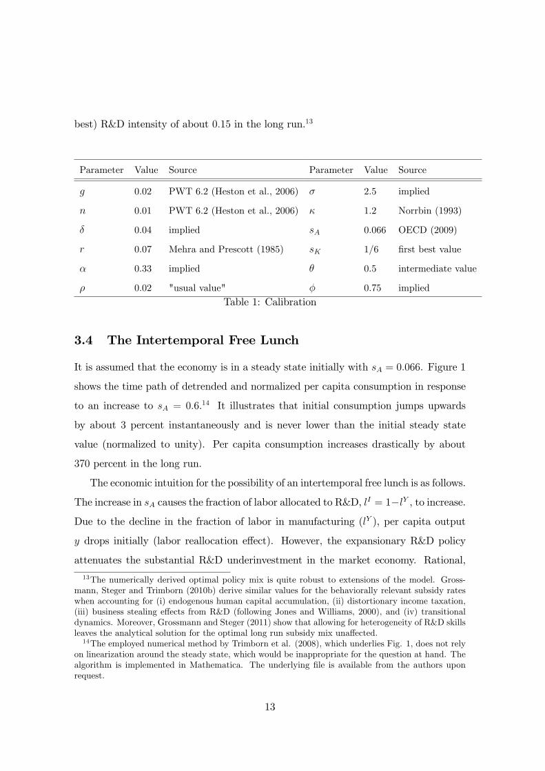
It is assumed that the economy is in a steady state initially with sA = 0.066. Figure 1

shows the time path of detrended and normalized per capita consumption in response

to an increase to sA = 0.6.14 It illustrates that initial consumption jumps upwards

by about 3 percent instantaneously and is never lower than the initial steady state

value (normalized to unity). Per capita consumption increases drastically by about

370 percent in the long run.

The economic intuition for the possibility of an intertemporal free lunch is as follows.

The increase in sA causes the fraction of labor allocated to R&D, lI = 1−lY , to increase.

Due to the decline in the fraction of labor in manufacturing (lY ), per capita output

y drops initially (labor reallocation effect). However, the expansionary R&D policy

attenuates the substantial R&D underinvestment in the market economy. Rational,

13The numerically derived optimal policy mix is quite robust to extensions of the model. Gross-mann, Steger and Trimborn (2010b) derive similar values for the behaviorally relevant subsidy rateswhen accounting for (i) endogenous human capital accumulation, (ii) distortionary income taxation,(iii) business stealing effects from R&D (following Jones and Williams, 2000), and (iv) transitionaldynamics. Moreover, Grossmann and Steger (2011) show that allowing for heterogeneity of R&D skillsleaves the analytical solution for the optimal long run subsidy mix unaffected.14The employed numerical method by Trimborn et al. (2008), which underlies Fig. 1, does not rely

on linearization around the steady state, which would be inappropriate for the question at hand. Thealgorithm is implemented in Mathematica. The underlying file is available from the authors uponrequest.

13

forward-looking agents understand that there is an associated wealth effect. They

therefore reduce the fraction of output devoted to the accumulation of physical capital,

i.e. inv decreases. Consequently, the rate of consumption, q = 1 − inv, rises. If the

increase in q(0) is large relative to the decrease in initial per capita income, y(0), per

capita consumption c(0) = q(0)y(0) may jump up initially.

Figure 1: The intertemporal free lunch

Notice that the Jones (1995) model fulfills the conditions of Proposition 1: (i) raising

the R&D subsidy affects the accumulation of knowledge, (ii) there are two degrees of

freedom in the allocation variables. Also the presumption of Proposition 1 holds, as

the optimal long run R&D subsidy is positive.

How does the proportional initial change of consumption (the 3 percent in the ex-

ample considered above) depend on the policy instrument sA? To see this, consider the

initial (i.e. at t = 0) rate of change of detrended per capita consumption, ∆c(0)/c(0),

in response to a change in sA from sA = 0.066 to sA ∈ [0.066 − 0.3, 0.066 + 0.85]. By

construction, at initial (US) value sA = 0.066, we have ∆c(0) = 0. Figure 2 (a) shows

∆c(0)/c(0) as function of the R&D subsidy. It shows that ∆c(0)/c(0) is rising in sA

up to sA = 0.72 and is negative for sA−increases slightly beyond the socially optimally

rate, i.e. for sA > 0.89.15

15The range of sA-increases which generate an increase in c(0) is smaller when the initial R&Dunderinvestment problem is less severe. For instance, if the "duplication externality" is parameterizedby θ = 0.75, the steady state R&D intensity at the socially optimal R&D subsidy rate is 7.9 percent(rather than 15 percent in the case where θ = 0.5). In this case, c(0) becomes negative for increasesin sA to a level which is considerably smaller than the socially optimal rate (not shown). However,qualitatively, the insights from Figure 2 remain valid.

14

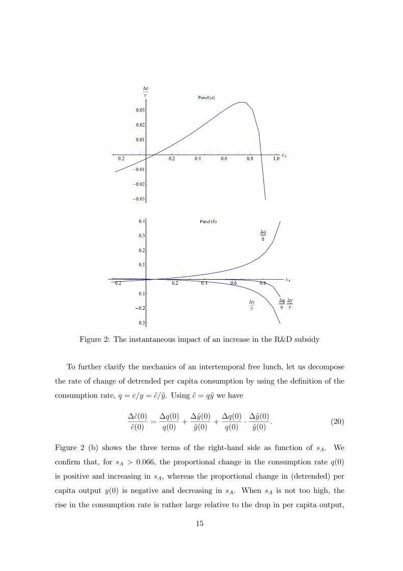
Figure 2: The instantaneous impact of an increase in the R&D subsidy

To further clarify the mechanics of an intertemporal free lunch, let us decompose

the rate of change of detrended per capita consumption by using the definition of the

consumption rate, q = c/y = c/y. Using c = qy we have

∆c(0)

c(0)=∆q(0)

q(0)+∆y(0)

y(0)+∆q(0)

q(0)·∆y(0)

y(0). (20)

Figure 2 (b) shows the three terms of the right-hand side as function of sA. We

confirm that, for sA > 0.066, the proportional change in the consumption rate q(0)

is positive and increasing in sA, whereas the proportional change in (detrended) per

capita output y(0) is negative and decreasing in sA. When sA is not too high, the

rise in the consumption rate is rather large relative to the drop in per capita output,

15

implying ∆c(0) > 0.

4 Dynamic Inefficiency and Endogenous Growth

This section briefly discusses whether alternative, widely-used endogenous growth mod-

els satisfy the necessary conditions for dynamic inefficiency, as listed in Proposition 1.

4.1 Lab-equipment Approach

Romer and Rivera-Batiz (1991) propose a R&D-based growth model which differs

from the set up analyzed in the previous section with respect to the R&D technology.

Horizontal innovations occur according to

A = ηY I − δIA, (21)

where Y I is the amount of final output used for knowledge accumulation. Capturing

the R&D process in this way is sometimes labelled as "lab-equipment approach".16

Labor is used for producing final output only, i.e., in equilibrium lY = 1. We can now

distinguish between three income shares to represent the use of income:

q + inv + sI = 1. (22)

The model fulfills conditions (i) and (ii) in Proposition 1 such that dynamic in-

efficiency may occur. For instance, an increase in the capital cost subsidy raises the

aggregate investment rate into physical capital, inv. If, at the same time, the R&D

investment rate, sI = Y I/Y , declines due to a wealth effect similar to the one discussed

above, then the net effect on the initial consumption rate, q(0), may be positive. If it

is, per capita consumption c(0) would increase since per capita output is not affected

instantaneously after a policy intervention. Thus, an intertemporal free lunch may be

16According to the classification in section 2, in contrast to the Jones (1995) model, the approachconstitutes a one-sector model. Only final output is used in the accumulation processes.

16

possible.

4.2 Learning-by-doing

We next consider learning-by-doing externalities à la Arrow (1962) and Romer (1986).

For illustrative purposes, consider the following production function of a representative

final goods producer:

Y = Aa(KY)α(LY )1−α, (23)

0 < α < 1, A > 0, where productivity measure a :=(KY)β, β > 0, is taken as given

by the Y−sector and driven by the aggregate capital input, KY . The assumption

captures that final goods producers do not take into account that capital investment

raises the economy-wide capital stock and therefore enhances total factor productivity.

This "learning-by-doing" externality distorts accumulation of the only capital good

downwards. With endogenous investment rate s, capital accumulates according to

K = sY − δK, δ > 0. There is no other sector such that, in equilibrium, KY = K and

LY = N (full employment conditions). For instance, if total labor supply N = 1 and

β = 1− α, the social production function is Y = AK ("AK-model").

The consumption rate reads q = 1− s. Now, addressing the externality by a policy

intervention which raises s leaves per capita output initially unaffected but inevitably

lowers q(0). Thus, an intertemporal free lunch is not possible and, by design, the

economy is dynamically efficient. Relating the insight to Proposition 1, note that there

is only one degree of freedom in the allocation variables. That is, V = 4 and R = 3

(full employment conditions and final goods market clearing). Thus, condition (ii) of

Proposition 1 is violated.

Whether the model is interpreted to encompass one or two accumulable input fac-

tors would not change the conclusion. One may consider TFP, as given by a := Kβ

(let A = 1), as the second accumulable factor such that a = βKβ−1K. However, this

model version still violates condition (ii) of Proposition 1. It illustrates that the exis-

tence of two degrees of freedom is indeed necessary for an intertemporal free lunch to

be realized, even in the case with two accumulable factors (I = 2).

17

4.3 Human Capital Externalities

Finally, consider human capital externalities à la Uzawa (1965) and Lucas (1988). Let

the production technology for final output be a function of both physical capital (K)

and human capital (H) such that Y = b(KY)α(HY )1−α, 0 < α < 1. The per capita

amount of human capital in the economy is denoted by h. There is a human capital

externality which drives total factor productivity, b := hγ, γ > 0. Unlike in the previous

examples, now the accumulation process of human capital uses neither final output nor

a non-accumulable factor but human capital itself. The education technology reads

h = ξ(hH)η− δHh, (24)

ξ > 0, η > 0, δH ≥ 0, where hH is the per capita level of human capital devoted to

education.17 The associated resource constraint reads

hH + hY = h, (25)

where hY is the per capita level of human capital devoted to final goods production.

Physical capital accumulation is standard in its exclusive use of final output; we have

K = sY − δKK, δK ≥ 0. Thus, the consumption rate again reads q = 1− s.

The Lucas-Uzawa model fulfills the necessary conditions for an intertemporal free

lunch mentioned in Proposition 1. There are two accumulable factors, namelyK and h.

Moreover, there are five allocation variables (KY , s, q, hH , hY ) and three constraints,

namely KY = K, s + q = 1 and (25), such that there are two degrees of freedom in

the allocation variables. Due to the human capital externality (γ > 0), an education

subsidy, which raises hH , may be justified. However, this inevitably reduces initial

per capita output y(0), in view of constraint (25). Nonetheless, it may be that, at

the same time, the education subsidy induces a wealth effect which leads to a decline

in investment rate s. Consequently, an instantaneous increase in the consumption

17Lucas (1988) implicitly assumes constant returns in the education technology, η = 1, which allowsfor sustained endogenous growth.

18

rate, q(0), is possible and may be high enough to raise the initial level of per capita

consumption, c(0) = q(0)y(0).

5 Conclusion

This paper has identified necessary conditions of dynamic inefficiency in the widely-

used class of dynamic, general equilibrium, infinite-horizon models with optimizing

agents even in a situation with long run underinvestment in an accumulable factor.

To the best of our knowledge, the possibility to realize an intertemporal free lunch in

such a framework has not been discussed in the previous literature. Our paper aims

to fill this gap. In order to dynamically evaluate policy interventions, researchers have

to be aware whether they are employing a framework where the possibility of dynamic

inefficiency is built-in or not.

We illustrated the possibility of an intertemporal free lunch in a standard, gen-

eral equilibrium model à la Jones (1995) with R&D-based, semi-endogenous, long run

growth and accumulation of physical capital. Interestingly, although the long run

rate of economic growth is not policy-dependent in the analyzed framework, we find

that the US economy underinvests in R&D and is dynamically inefficient. That is,

TANSTAAFL does not apply. At the first glance, this seems surprising. A priori, one

would suspect that mitigating the R&D underinvestment problem requires to give up

consumption at least in the short run. We showed that this is not the case when the

R&D subsidy rate is raised, due to an immediate slowdown in the process of capital

accumulation.

In sum, our analysis suggests that dynamic inefficiency is not a theoretical anom-

aly even in models with fully optimizing, infinitely-lived, forward-looking agents and

positive investment externalities. It is not often that economists can make such strong

policy recommendations than in the case of dynamic inefficiency. Thus, future work

should further investigate this fascinating issue in order to help realizing possible in-

tertemporal free lunches.

19

References

[1] Abel, Andrew, Gregory M. Mankiw, Lawrence H. Summers and Richard J. Zeck-

hauser (1989). Assessing Dynamic Efficiency: Theory and Evidence, Review of

Economic Studies 56, 1-19.

[2] Arrow, Kenneth J. (1962). The Economic Implications of Learning By Doing,

Review of Economic Studies 29, 155-173.

[3] Friedman, Milton (1975). There’s No Such Thing as a Free Lunch, LaSalle, Ill.:

Open Court.

[4] Grossmann, Volker, Thomas M. Steger and Timo Trimborn (2010a). Dynamically

Optimal R&D Subsidization, CESifo Working Paper No. 3153.

[5] Grossmann, Volker, Thomas M. Steger and Timo Trimborn (2010b). Quantifying

Optimal Growth Policy, CESifo Working Paper No. 3092.

[6] Grossmann, Volker and Thomas M. Steger (2011). Optimal Policy Towards

Growth and Innovation: The Role of Skill Heterogeneity, University of Fribourg

and Leipzig (mimeo).

[7] Heston, Alan, Robert Summers and Bettina Aten (2006). Penn World Table Ver-

sion 6.2, Center for International Comparisons of Production, Income and Prices

at the University of Pennsylvania.

[8] Jones, Charles I. (1995). R&D-based Models of Economic Growth, Journal of

Political Economy 103, 759—784.

[9] Jones, Charles I. and John C. Williams (2000). Too Much of a Good Thing? The

Economics of Investment in R&D, Journal of Economic Growth 5, 65-85.

[10] Lucas, Robert E. (1988). On the Mechanics of Economic Development, Journal of

Monetary Economics 22, 3-42.

20

[11] Mankiw, N. Gregory, David Romer and David N. Weil (1992). A Contribution to

the Empirics of Economic Growth, Quarterly Journal of Economics 107, 407-437.

[12] Mehra, Rajnish and Edward C. Prescott (1985). The Equity Premium: A Puzzle,

Journal of Monetary Economics 15, 145-61.

[13] Norrbin, Stefan C. (1993). The Relationship Between Price and Marginal Cost in

U.S. Industry: A Contradiction, Journal of Political Economy 101, 1149-1164.

[14] OECD (2009). Science Technology and Industry Scoreboard 2009, Paris.

[15] Phelps, Edmund S. (1966). Golden Rules of Economic Growth, New York: W.W.

Norton.

[16] Romer, Paul M. (1986). Increasing Returns and Long-run Growth, Journal of

Political Economy 94, 1002-1037.

[17] Romer, Paul M. and Luis A. Rivera-Batiz (1991). Economic Integration and En-

dogenous Growth, Quarterly Journal of Economics 106, 531-555.

[18] Trimborn, Timo, Karl-Josef Koch and Thomas M. Steger (2008). Multi-

Dimensional Transitional Dynamics: A Simple Numerical Procedure, Macroeco-

nomic Dynamics 12, 301—319.

21

Universität Leipzig Wirtschaftswissenschaftliche Fakultät

Nr. 1 Wolfgang Bernhardt Stock Options wegen oder gegen Shareholder Value? Vergütungsmodelle für Vorstände und Führungskräfte 04/1998

Nr. 2 Thomas Lenk / Volkmar Teichmann Bei der Reform der Finanzverfassung die neuen Bundesländer nicht vergessen! 10/1998

Nr. 3 Wolfgang Bernhardt Gedanken über Führen – Dienen – Verantworten 11/1998

Nr. 4 Kristin Wellner Möglichkeiten und Grenzen kooperativer Standortgestaltung zur Revitalisierung von Innenstädten 12/1998

Nr. 5 Gerhardt Wolff Brauchen wir eine weitere Internationalisierung der Betriebswirtschaftslehre? 01/1999

Nr. 6 Thomas Lenk / Friedrich Schneider Zurück zu mehr Föderalismus: Ein Vorschlag zur Neugestaltung des Finanzausgleichs in der Bundesrepublik Deutschland unter besonderer Berücksichtigung der neuen Bundesländer 12/1998

Nr: 7 Thomas Lenk Kooperativer Förderalismus – Wettbewerbsorientierter Förderalismus 03/1999

Nr. 8 Thomas Lenk / Andreas Mathes EU – Osterweiterung – Finanzierbar? 03/1999

Nr. 9 Thomas Lenk / Volkmar Teichmann Die fisikalischen Wirkungen verschiedener Forderungen zur Neugestaltung des Länderfinanz-ausgleichs in der Bundesrepublik Deutschland: Eine empirische Analyse unter Einbeziehung der Normenkontrollanträge der Länder Baden-Würtemberg, Bayern und Hessen sowie der Stellungnahmen verschiedener Bundesländer 09/1999

Nr. 10 Kai-Uwe Graw Gedanken zur Entwicklung der Strukturen im Bereich der Wasserversorgung unter besonderer Berücksichtigung kleiner und mittlerer Unternehmen 10/1999

Nr. 11 Adolf Wagner Materialien zur Konjunkturforschung 12/1999

Nr. 12 Anja Birke Die Übertragung westdeutscher Institutionen auf die ostdeutsche Wirklichkeit – ein erfolg-versprechendes Zusammenspiel oder Aufdeckung systematischer Mängel? Ein empirischer Bericht für den kommunalen Finanzausgleich am Beispiel Sachsen 02/2000

Nr. 13 Rolf H. Hasse Internationaler Kapitalverkehr in den letzten 40 Jahren – Wohlstandsmotor oder Krisenursache? 03/2000

Nr. 14 Wolfgang Bernhardt Unternehmensführung (Corporate Governance) und Hauptversammlung 04/2000

Nr. 15 Adolf Wagner Materialien zur Wachstumsforschung 03/2000

Nr. 16 Thomas Lenk / Anja Birke Determinanten des kommunalen Gebührenaufkommens unter besonderer Berücksichtigung der neuen Bundesländer 04/2000

Nr. 17 Thomas Lenk Finanzwirtschaftliche Auswirkungen des Bundesverfassungsgerichtsurteils zum Länderfinanzausgleich vom 11.11.1999 04/2000

Nr. 18 Dirk Bültel Continous linear utility for preferences on convex sets in normal real vector spaces 05/2000

Nr. 19 Stefan Dierkes / Stephanie Hanrath Steuerung dezentraler Investitionsentscheidungen bei nutzungsabhängigem und nutzungsunabhängigem Verschleiß des Anlagenvermögens 06/2000

Nr. 20 Thomas Lenk / Andreas Mathes / Olaf Hirschefeld Zur Trennung von Bundes- und Landeskompetenzen in der Finanzverfassung Deutschlands 07/2000

Nr. 21 Stefan Dierkes Marktwerte, Kapitalkosten und Betafaktoren bei wertabhängiger Finanzierung 10/2000

Nr. 22 Thomas Lenk Intergovernmental Fiscal Relationships in Germany: Requirement for New Regulations? 03/2001

Nr. 23 Wolfgang Bernhardt Stock Options – Aktuelle Fragen Besteuerung, Bewertung, Offenlegung 03/2001

Nr. 24 Thomas Lenk Die „kleine Reform“ des Länderfinanzausgleichs als Nukleus für die „große Finanzverfassungs-reform“? 10/2001

Nr. 25 Wolfgang Bernhardt Biotechnologie im Spannungsfeld von Menschenwürde, Forschung, Markt und Moral Wirtschaftsethik zwischen Beredsamkeit und Schweigen 11/2001

Nr. 26 Thomas Lenk Finanzwirtschaftliche Bedeutung der Neuregelung des bundestaatlichen Finanzausgleichs – Eine allkoative und distributive Wirkungsanalyse für das Jahr 2005 11/2001

Nr. 27 Sören Bär Grundzüge eines Tourismusmarketing, untersucht für den Südraum Leipzig 05/2002

Nr. 28 Wolfgang Bernhardt Der Deutsche Corporate Governance Kodex: Zuwahl (comply) oder Abwahl (explain)? 06/2002

Nr. 29 Adolf Wagner Konjunkturtheorie, Globalisierung und Evolutionsökonomik 08/2002

Nr. 30 Adolf Wagner Zur Profilbildung der Universitäten 08/2002

Nr. 31 Sabine Klinger / Jens Ulrich / Hans-Joachim Rudolph

Konjunktur als Determinante des Erdgasverbrauchs in der ostdeutschen Industrie? 10/2002

Nr. 32 Thomas Lenk / Anja Birke The Measurement of Expenditure Needs in the Fiscal Equalization at the Local Level Empirical Evidence from German Municipalities 10/2002

Nr. 33 Wolfgang Bernhardt Die Lust am Fliegen Eine Parabel auf viel Corporate Governance und wenig Unternehmensführung 11/2002

Nr. 34 Udo Hielscher Wie reich waren die reichsten Amerikaner wirklich? (US-Vermögensbewertungsindex 1800 – 2000) 12/2002

Nr. 35 Uwe Haubold / Michael Nowak Risikoanalyse für Langfrist-Investments Eine simulationsbasierte Studie 12/2002

Nr. 36 Thomas Lenk Die Neuregelung des bundesstaatlichen Finanzausgleichs auf Basis der Steuerschätzung Mai 2002 und einer aktualisierten Bevölkerungsstatistik 12/2002

Nr. 37 Uwe Haubold / Michael Nowak Auswirkungen der Renditeverteilungsannahme auf Anlageentscheidungen Eine simulationsbasierte Studie 02/2003

Nr. 38 Wolfgang Bernhard Corporate Governance Kondex für den Mittel-Stand? 06/2003

Nr. 39 Hermut Kormann Familienunternehmen: Grundfragen mit finanzwirtschaftlichen Bezug 10/2003

Nr. 40 Matthias Folk Launhardtsche Trichter 11/2003

Nr. 41 Wolfgang Bernhardt Corporate Governance statt Unternehmensführung 11/2003

Nr. 42 Thomas Lenk / Karolina Kaiser Das Prämienmodell im Länderfinanzausgleich – Anreiz- und Verteilungsmitwirkungen 11/2003

Nr. 43 Sabine Klinger Die Volkswirtschaftliche Gesamtrechnung des Haushaltsektors in einer Matrix 03/2004

Nr. 44 Thomas Lenk / Heide Köpping Strategien zur Armutsbekämpfung und –vermeidung in Ostdeutschland: 05/2004

Nr. 45 Wolfgang Bernhardt Sommernachtsfantasien Corporate Governance im Land der Träume. 07/2004

Nr. 46 Thomas Lenk / Karolina Kaiser The Premium Model in the German Fiscal Equalization System 12/2004

Nr. 47 Thomas Lenk / Christine Falken Komparative Analyse ausgewählter Indikatoren des Kommunalwirtschaftlichen Gesamt-ergebnisses 05/2005

Nr. 48 Michael Nowak / Stephan Barth Immobilienanlagen im Portfolio institutioneller Investoren am Beispiel von Versicherungsunternehmen Auswirkungen auf die Risikosituation 08/2005

Nr. 49 Wolfgang Bernhardt Familiengesellschaften – Quo Vadis? Vorsicht vor zu viel „Professionalisierung“ und Ver-Fremdung 11/2005

Nr. 50 Christian Milow Der Griff des Staates nach dem Währungsgold 12/2005

Nr. 51 Anja Eichhorst / Karolina Kaiser The Instiutional Design of Bailouts and Its Role in Hardening Budget Constraints in Federations 03/2006

Nr. 52 Ullrich Heilemann / Nancy Beck Die Mühen der Ebene – Regionale Wirtschaftsförderung in Leipzig 1991 bis 2004 08/2006

Nr. 53 Gunther Schnabl Die Grenzen der monetären Integration in Europa 08/2006

Nr. 54 Hermut Kormann Gibt es so etwas wie typisch mittelständige Strategien? 11/2006

Nr. 55 Wolfgang Bernhardt (Miss-)Stimmung, Bestimmung und Mitbestimmung Zwischen Juristentag und Biedenkopf-Kommission 11/2006

Nr. 56 Ullrich Heilemann / Annika Blaschzik Indicators and the German Business Cycle A Multivariate Perspective on Indicators of lfo, OECD, and ZEW 01/2007

Nr. 57 Ullrich Heilemann “The Suol of a new Machine” zu den Anfängen des RWI-Konjunkturmodells 12/2006

Nr. 58 Ullrich Heilemann / Roland Schuhr / Annika Blaschzik

Zur Evolution des deutschen Konjunkturzyklus 1958 bis 2004 Ergebnisse einer dynamischen Diskriminanzanalyse 01/2007

Nr. 59 Christine Falken / Mario Schmidt Kameralistik versus Doppik Zur Informationsfunktion des alten und neuen Rechnungswesens der Kommunen Teil I: Einführende und Erläuternde Betrachtungen zum Systemwechsel im kommunalen Rechnungswesen 01/2007

Nr. 60 Christine Falken / Mario Schmidt Kameralistik versus Doppik Zur Informationsfunktion des alten und neuen Rechnungswesens der Kommunen Teil II Bewertung der Informationsfunktion im Vergleich 01/2007

Nr. 61 Udo Hielscher Monti della citta di firenze Innovative Finanzierungen im Zeitalter Der Medici. Wurzeln der modernen Finanzmärkte 03/2007

Nr. 62 Ullrich Heilemann / Stefan Wappler Sachsen wächst anders Konjunkturelle, sektorale und regionale Bestimmungsgründe der Entwicklung der Bruttowertschöpfung 1992 bis 2006 07/2007

Nr. 63 Adolf Wagner Regionalökonomik: Konvergierende oder divergierende Regionalentwicklungen 08/2007

Nr. 64 Ullrich Heilemann / Jens Ulrich Good bye, Professir Phillips? Zum Wandel der Tariflohndeterminanten in der Bundesrepublik 1952 – 2004 08/2007

Nr. 65 Gunther Schnabl / Franziska Schobert Monetary Policy Operations of Debtor Central Banks in MENA Countries 10/2007

Nr. 66 Andreas Schäfer / Simone Valente Habit Formation, Dynastic Altruism, and Population Dynamics 11/2007

Nr. 67 Wolfgang Bernhardt 5 Jahre Deutscher Corporate Governance Kondex Eine Erfolgsgeschichte? 01/2008

Nr. 68 Ullrich Heilemann / Jens Ulrich Viel Lärm um wenig? Zur Empirie von Lohnformeln in der Bundesrepublik 01/2008

Nr. 69 Christian Groth / Karl-Josef Koch / Thomas M. Steger When economic growth is less than exponential 02/2008

Nr. 70 Andreas Bohne / Linda Kochmann Ökonomische Umweltbewertung und endogene Entwicklung peripherer Regionen Synthese einer Methodik und einer Theorie 02/2008

Nr. 71 Andreas Bohne / Linda Kochmann / Jan Slavík / Lenka Slavíková

Deutsch-tschechische Bibliographie Studien der kontingenten Bewertung in Mittel- und Osteuropa 06/2008

Nr. 72 Paul Lehmann / Christoph Schröter-Schlaack Regulating Land Development with Tradable Permits: What Can We Learn from Air Pollution Control? 08/2008

Nr. 73 Ronald McKinnon / Gunther Schnabl China’s Exchange Rate Impasse and the Weak U.S. Dollar 10/2008

Nr: 74 Wolfgang Bernhardt Managervergütungen in der Finanz- und Wirtschaftskrise Rückkehr zu (guter) Ordnung, (klugem) Maß und (vernünftigem) Ziel? 12/2008

Nr. 75 Moritz Schularick / Thomas M. Steger Financial Integration, Investment, and Economic Growth: Evidence From Two Eras of Financial Globalization 12/2008

Nr. 76 Gunther Schnabl / Stephan Freitag An Asymmetry Matrix in Global Current Accounts 01/2009

Nr. 77 Christina Ziegler Testing Predictive Ability of Business Cycle Indicators for the Euro Area 01/2009

Nr. 78 Thomas Lenk / Oliver Rottmann / Florian F. Woitek Public Corporate Governance in Public Enterprises Transparency in the Face of Divergent Positions of Interest 02/2009

Nr. 79 Thomas Steger / Lucas Bretschger Globalization, the Volatility of Intermediate Goods Prices, and Economic Growth 02/2009

Nr. 80 Marcela Munoz Escobar / Robert Holländer Institutional Sustainability of Payment for Watershed Ecosystem Services. Enabling conditions of institutional arrangement in watersheds 04/2009

Nr. 81 Robert Holländer / WU Chunyou / DUAN Ning Sustainable Development of Industrial Parks 07/2009

Nr. 82 Georg Quaas Realgrößen und Preisindizes im alten und im neuen VGR-System 10/2009

Nr. 83 Ullrich Heilemann / Hagen Findeis Empirical Determination of Aggregate Demand and Supply Curves: The Example of the RWI Business Cycle Model 12/2009

Nr. 84 Gunther Schnabl / Andreas Hoffmann The Theory of Optimum Currency Areas and Growth in Emerging Markets 03/2010

Nr. 85 Georg Quaas Does the macroeconomic policy of the global economy’s leader cause the worldwide asymmetry in current accounts? 03/2010

Nr. 86 Volker Grossmann / Thomas M. Steger / Timo Trimborn Quantifying Optimal Growth Policy 06/2010

Nr. 87 Wolfgang Bernhardt Corporate Governance Kodex für Familienunternehmen? Eine Widerrede 06/2010

Nr. 88 Philipp Mandel / Bernd Süssmuth A Re-Examination of the Role of Gender in Determining Digital Piracy Behavior 07/2010

Nr. 89 Philipp Mandel / Bernd Süssmuth Size Matters. The Relevance and Hicksian Surplus of Agreeable College Class Size 07/2010

Nr. 90 Thomas Kohstall / Bernd Süssmuth Cyclic Dynamics of Prevention Spending and Occupational Injuries in Germany: 1886-2009 07/2010

Nr. 91 Martina Padmanabhan Gender and Institutional Analysis. A Feminist Approach to Economic and Social Norms 08/2010

Nr. 92 Gunther Schnabl /Ansgar Belke Finanzkrise, globale Liquidität und makroökonomischer Exit 09/2010

Nr. 93 Ullrich Heilemann / Roland Schuhr / Heinz Josef Münch A “perfect storm”? The present crisis and German crisis patterns 12/2010

Nr. 94 Gunther Schnabl / Holger Zemanek Die Deutsche Wiedervereinigung und die europäische Schuldenkrise im Lichte der Theorie optimaler Währungsräume 06/2011

Nr. 95 Andreas Hoffmann / Gunther Schnabl Symmetrische Regeln und asymmetrisches Handeln in der Geld- und Finanzpolitik 07/2011

Nr. 96 Andreas Schäfer / Maik T. Schneider Endogenous Enforcement of Intellectual Property, North-South Trade, and Growth 08/2011

Nr. 97 Volker Grossmann / Thomas M. Steger / Timo Trimborn Dynamically Optimal R&D Subsidization 08/2011

Nr. 98 Erik Gawel Political drivers of and barriers to Public-Private Partnerships: The role of political involvement 09/2011

Nr. 99 André Casajus Collusion, symmetry, and the Banzhaf value 09/2011

Nr. 100 Frank Hüttner / Marco Sunder Decomposing R2 with the Owen value 10/2011

Nr. 101 Volker Grossmann / Thomas M. Steger / Timo Trimborn The Macroeconomics of TANSTAAFL 11/2011